Embed Size (px)
Citation preview

Student Spring 2016 Master thesis, 15 ETS Master Program in Economics
Impact of firm characteristics on wages Industry wage differentials and firm size-wage effects in Sweden
Xiaoying Li

Acknowledgments
I would like to express my appreciation to the lectures and professors from the
Department of Economics of Umeå University, who make me have the interests and
enthusiasm to deeply study and investigate the aspect of Labor Economics: wage
distribution, and the factors that influence wages. Besides, I am greatly grateful to my
supervisor Katharina Jenderny, who provided detail and helpful suggestion during the
whole thesis process. At last, I am particularly thanks to Swedish National Data
Service, for their help with collecting the data.
Abstract
Wage structure has shown to be crucial for firms and workers. However, there exist
wage dispersion for identical workers in labor markets. The paper measures the effect
of industry and firm size on wages in Sweden. The results show that both industry and
firm size have significant effects on wages. Regarding the explanation factors, the
finding is that human capital factors can explain a portion of the industry wage
differentials, but have less impact on wage differentials across firm size. However,
compensating differentials and union organization are not the determinants of the
industry wage differentials and firm size-wage effects. In addition, unobserved
individual characteristics can partly explain firm size effect on wages, but cannot
explain industry wage differentials based on our samples.
Key words: wage dispersion; inter-industry wage differentials; firm size-wage effects
Table of Contents
1. Introduction........................................................................................................................................1
2. Theory and Literature reviews.....................................................................................................3
2.1 Impact of firm characteristics on wages.......................................................................3
2.2 Explanations for wage dispersion across industries and firm size......................4
2.3 Wage policy and evidence in Sweden..........................................................................8
3. Data....................................................................................................................................................11
4. Econometric model......................................................................................................................15
5. Results...........................................................................................................................................18
5.1 Estimating inter-industry wage differentials and size-wage effects................19
5.2 Testing explanations for industry wage differentials and size-wage effects 20
5.3 Summary..............................................................................................................................27
6. Concluding Remarks...................................................................................................................29
References............................................................................................................................................30
Appendix..............................................................................................................................................34
1
1. Introduction
In the labor market, wages can reflect marginal revenue productivity for firms (Rosen,
1986; Feldstein, 2008), and wages can motivate their workers to make effort (Gruette
and Lalive, 2009). However, low wages will help firms promote cost savings. For
workers, wages can determine their quality of life; individuals who earn high wages
can afford better lifestyles than those who get lower wages. Furthermore, wages play
an important role in determining of job changing decisions (Topel and Ward, 1992).
Thus, wage structure has shown to be crucial for firms and workers. It is useful to find
the factors that affect wages in the long run.
There exist wage dispersion for identical workers doing equivalent jobs in labor
markets (Erdil and Yetkner, 2001). A number of studies suggest that firm
characteristics are more important than individual effects in explaining wage
dispersions (Groshen, 1991; Davis and Haltiwanger, 1996; Kramarz et al., 1996). Oi
and Idson (1999) show that jobs can be categorized by occupation, industry,
ownership (public and private), geographic location, or employer size. Among these
factors, the inter-industry wage differentials and firm size wage differentials are two
key dispersions observed in the labor markets (Krueger and Summers, 1988; Brown
and Medoff, 1989; Morissette, 1993).
The purpose of this paper is to measure the effect of firm characteristics on wages in
Sweden. The characteristics relate to industry and firm size. Three research questions
are presented as follows:
(1) How do wages vary across industries?
(2) How does firm size influence wages?
(3) What can explain the wage differential across industries and firm size?
In this paper, data is collected from the Household market and nonmarket activities
(HUS) survey in 1996 and 1998. First, I estimate the wage equation by the Ordinary
least squares (OLS) to evaluate the effects of industry and firm size on wages. Human
capital factors, compensating differentials, and union organization are also included in
the model to test their explanations for wage differentials across industries and firm

2
size. In addition, I use panel data fixed effects model to control for unobserved
personal characteristics.
The major finding is that there exist industry wage differentials without other control
variables. High wage jobs are to be found in industries such as banking and other
financial business, real estate management, and manufacturing. Wages are lower in
traditional industries like farming, restaurant and hotel, as well as lumber production.
Besides, firm size has a positive statistically significant impact on wages; large firms
pay higher wages than small firms. The results indicate that human capital factors can
partly explain the industry wage differentials, but have less impact on wage dispersion
across firm size. However, compensating differentials and union organization have no
effect to change the industry wage differentials and firm size-wage effect. Moreover,
unobserved individual characteristics can explain a portion of firm size effect on
wages, but seem not to explain wage differential across industries based on our
samples.
The paper is organized as follows. Section 2 reviews related theory and literature
about inter-industry wage differentials and firm size effects. Section 3 and Section 4
introduce the data and the econometric model used in this paper, respectively. Section
5 presents the results from the empirical regression. The final section concludes this
paper.
3
2. Theory and Literature reviews In this section, I will first review existing evidence for the impact of industry and firm
size on wage levels. Then I will review wage dispersion theory (Mortensen, 2003) and
other different explanations for the effect of industry and firm size on wages. At last, I
will describe the wage policy and previous studies for Sweden.
2.1 Impact of firm characteristics on wages
2.1.1 Evidence for industry wage differentials
There is substantial evidence regarding industry wage differentials. Krueger and
Summers (1988) use data from the Current Population Survey for May 1974, 1979,
and 1984 to measure the wage variability across industries. They find that industry
has a large impact on employee’s wage in the United States, even after controlling for
human capital and other job characteristics. When industry dummies are included in
the regression, the standard error of the regression (the average distance that the
observed values fall from the estimated regression line) decreases by 4.3 percentage
points. Goux and Maurin (1999) find that two individuals get substantial different
income due to the industries where they are hired. The study is based on a panel of
matched employer-employee data in France from 1990 to 1995. They find that wages
are lower in traditional industries, such as bakeries, food retailing, as well as the hotel
industry. However, the high wage industries contain air transportation, oil,
pharmaceuticals, and mining. Moreover, Carruth et al. (2004) estimate inter-industry
wage differentials in Britain with micro-data over the period 1991-1998. Their finding
also suggests a small but statistically significant industry effect on wage differentials.
Besides, inter-industry wage differentials are compared in different countries. Using
longitudinal census data, Vainiomäki and Laaksonen (1995) suggest that there exist
eight percent industry wage differentials after controlling for human capital and job
factors in Finland during 1975-1985, which is larger than in Sweden but smaller than
in the United States. Alback et al. (1996) evaluate wage differentials across the
Nordic countries. They conclude that wage dispersion between countries is less than
the dispersion across industries. Furthermore, Genre et al. (2011) select a panel of 22
industries across eight Euro countries in 1991-2002. They find large and stable
inter-industry wage differentials in the Euro area countries.
4
2.1.2 Evidence for firm size-wage effects
A large number of studies provide evidence for firm size-wage effects. Schmidt and
Zimmermann (1991) using data from a random survey of individuals find that wages
increase significantly with firm size in Germany in 1978, even after controlling for
human capital, job characteristics, and demographic characteristic. Consistent with
Schmidt and Zimmermann’s finding, Morissette (1993) concludes that larger firms
pay higher wages than smaller firms, and the wage differential on firm size is large in
Canada during 1986. Additionally, Waddoups (2007) using data over 1993-2001
confirms that Australia has a positive significant employer size-wage effect. For
males, compared with workers employed in firms with less than 10 employees,
workers employed in firms with more than 100 employees get nearly 25 percent
higher wages.
However, this positive size-wage relation cannot be shown in China. Gao and Smyth
(2011) use a matched employee-employer data set in 2007; they suggest that firm size
has a negative statistically significant relationship to wages in Shanghai, after
controlling for firm’s ownership and several employee factors like the year of
schooling, experience, and gender. But when adding the ratio of blue-collar workers1
in the model, the negative relationship changes to statistically insignificant. The
possible explanation for the negative size-wage relationship in China is that larger
firms employ more blue-collar workers than smaller firms. Moreover, Belfield and
Wei (2004) claim that firms with more blue-collar workers do not have to pay higher
wages due to face with less labor turnover. Thus in China, larger firms paid lower
wages than smaller firms.
2.2 Explanations for wage dispersion across industries and firm size
2.2.1 Wage dispersion theory
How can these empirical findings be rationalized theoretically? First, Mortensen
(2003) provides a theoretical explanation for wage dispersion. He assumes that there
are fixed numbers of identical employers and identical workers in the market. The
hiring process between firms and workers has two stages. First, firms simultaneously 1 A blue-collar worker refers to an individual who performs manual labor. Their job may involve manufacturing, construction, and other types of physical work. In contrast, a white-collar worker is a person who performs the job in an office. They do such as professional, managerial, and administrative work (Mcconnell et al., 2009).
5
decide on a wage offer and send it to a random worker. Second, the worker accepts
the offer with the highest wage.
In the hiring game, firms compete to attract workers on the market. The sequence of
the firm’s strategy in the model is as follows:
1. The firm realizes that the worker can receive several wage offers and accept the
highest-paying one.
2. Based on the assumption that all the other firms’ offers are also received by the
worker, the firm decides to calculate the probability that its offer is accepted,
which requires its offer (w) is larger than all the other received offers.
3. The firm expects to get profit from hiring this worker; it implies the wage offered
(w) is not larger than the worker’s productivity (p).
4. The firm needs to use a mixed strategy to set a wage offer distribution F(w) to
maximize the profit (𝜋); the profit is equal to the probability that its offer is
accepted times the difference between the productivity and the wage paid to the
worker (p-w).
The theory argues that even when all employers are identical based on the assumption,
the only equilibrium solution to this game generates a wage offer distribution. Since
the firm can arbitrarily decide its wage policy, the theory gives an explanation for
wage dispersion.
Based on the wage dispersion theory, both inter-industry wage differentials and
size-wage effects can be derived theoretically if firms differ in productivity levels.
Mortensen (2003) shows that there is a positive relationship between the productivity
level and wage offer. The more productive firm offers a higher wage and makes a
larger profit simultaneously. Oi and Idson (1999) suggest that labor productivity can
vary across industries. Then due to the positive correlation between wage and
productivity, it can be inferred the same worker in industries with higher productivity
earn more. The industry has an impact on wage levels.
As regards the relation between firm size and wages, since a more productive firm get
larger profit as previously shown, then a more productive firm has an incentive to
6
attract more workers compared to a low productive firm. Thus, the more productive
firm contacts more workers. The firm size is expected to increase with the number of
workers contacted increases. Meanwhile, wages are also higher in the firm with more
productivity than in the firm with less productivity. Thus, the theory argues that both
firm size and wages have increasing trends with firm’s productivity rise, and then
wage has a positive but not perfect correlation with firm size.
In addition to the wage dispersion theory sketched above, several other factors may
explain inter-industry wage differentials and size-wage effects. The common
explanations include human capital factors, compensating differentials, union
organization, as well as unobserved individual characteristics. Some theoretical
arguments and empirical evidence regarding their determinant influence are
summarized as follows:
2.2.2 Human capital factors
Human capital theory indicates that individuals’ education and past training have a
positive impact on their wages (Boeri and Ours, 2013). The standard human capital
earnings’ factors are shown by Mincer (1974), which contain workers’ schooling
levels and working experience (substituted by age) as explanatory variables.
Furthermore, Blinder (1976) suggests job tenure can be used as the human capital
factor since it reflects working experience in the current job.
Since individuals working in the same industry may require similar skills, these
human capital differences may mainly transfer into industry differences (Erdil and
Yetner, 2001). Their empirical study finds that the capital-intensive industries like
petroleum and electronics are hiring more skilled workers to manage the capital than
labor-intensive industries such as food and beverages. Besides, Main and Reilly (1993)
using individual interviews find that workers hired in larger firms not only earn more
than workers hired in small firms but also are more educated and generate higher
labor experience than workers in small plants. However, as reviewed in Section 2.1
(Krueger and Summers, 1988; Schmidt and Zimmermann, 1991; Vainiomäki and
Laaksonen, 1995), industry and firm size still have the effect on wage levels after
7
controlling for human capitals, which implies human capital factors may not fully
explain inter-industry wage differentials and size-wage effects.
2.2.3 Compensating differentials
Rosen (1986) suggests the Hedonic wage function, in which wage has a positive
relationship with the probability that jobs containing disamenity. It implies employers
need to provide higher wages to attract workers with respect to jobs with bad working
conditions.
Logically, inter-industry wage differentials can be explained by compensating
differentials as working environments vary across industries. However, as shown in
previous part, compensating differentials are not playing a key role, as controls for
working conditions do not substantially reduce the inter-industry wage differentials
(Krueger and Summers, 1998). Regarding compensating wage differentials on
explaining size-wage effects, Masters (1969) suggests that working in larger firms is
less pleasant due to increased work division, impersonal atmosphere, and requires
workers to be more dependent on each other. However, Wagner (1997) shows that
there is general evidence showing that working conditions are worse in smaller firms
from a survey of the empirical evidence in Germany.
2.2.4 Union organization
Union organization plays a key role in bargaining for workers’ wages (Baker et al.,
1988). In order to get higher wages, wages are negotiated between a union and the
firm. Union organization has a large impact on wage levels.
Naylor (2003) suggests that unions can lead to higher wages for the represented
market segment and that unions are stronger in public services industries and
manufacturing industries than in private service industries. In general, a union is
much easier founded in large firms. In Belfield and Wei (2004) empirical analysis,
union membership reduces the employer size-wage effects when it is controlled for,
which implies the size-wage effect can be partly explained by union organization.
8
2.2.5 Unobserved individual characteristics
In addition, some empirical studies show that both industry wage differentials and
size-wage effects can be explained by unobserved individual characteristics. For
example, Krueger and Summers (1988) find that compared to human capital,
unmeasured personal quality plays a major role in determining the industry wage
differentials. Cai and Waddoups (2012) suggest that part of the firm size–wage effects
can be attributable to unobserved individual ability differences, the significant
positive relationship between firm size and wages substantially reduce when
controlling for unobserved individual quality differences. Moreover, Abowd et al.
(1999) show that almost 90% of industry wage differentials and 75% of the firm
size-wage effects can be explained by individual fixed effects.
2.3 Wage policy and evidence in Sweden
2.3.1 Swedish solidarity wage policy
Edin and Holmlund (1995) describe the Swedish Wage Structure. I review the
primary features of the wage structure as follows. The Swedish trade union
confederation (LO) and the Swedish employers’ federation (SAF) are two key
organizations in Swedish labor markets. In 1938, LO and SAF reached the “Basic
Agreement” Saltsjöbadsavtalet, which provided some rules for labor conflict
resolutions and built a foundation to get more peaceful labor relations. From the late
1930s, the solidarity wage policy was formed. It reflected demands for a more
centralized bargaining structure within LO. However, the probability of quickly
implementing such a policy in practice was low, because of coordination is a
necessary prerequisite step. LO’s economists Gösta Rehn and Rudolf Meidner
promoted the principle for the wage policy was “equal pay for equal work”. This
principle excluded wage differences due to the difference in firms’ profitability. It
implies wage is independent in paying ability among particular firms and industries.
The solidarity wage policy was the main element of “the Swedish model”. Wage
negotiations happened at three levels. During the 1950s, the national coordination of
wage negotiations has gradually appeared in practice. LO and SAF have come to
sixteen central framework agreements between 1956 and 1983. However, the metal
workers’ union kept away from the LO-SAF national negotiations and chose an

9
industry agreement in 1983. It represents a significant turning point toward the
decentralized wage negotiation. After 1983, the wage bargaining has primarily taken
place at the industry level. In the late 1990s, Industrial Agreement (IA) has been
formed, which was initiated by a few blue-collar unions in the manufacturing sector.
The agreement involved employer organizations, blue-collar and white-collar unions
in establishing rules around the schedule for negotiations, regulations for conflict
resolution. This implied a change towards more informal wage bargaining.
Meanwhile, the wage negotiation stronger shifted towards the local enterprise level.
Another feature of the Swedish labor market is the high degree of union membership.
Based on the results of labor force surveys, union density reached 81 percent in 1991.
Union participation rate is higher in the public sector than in the private sector.
2.3.2 Previous evidence for Sweden
Regarding industry effects in Sweden, Edin and Zetterberg (1992) considering data
from the 1984 Household Market and Nonmarket Activities (HUS) survey, find that
the inter-industry wage differentials in Sweden are much smaller than in the United
States. A large part of the industry wage differentials in Sweden is due to industry
differences in labor quality and working conditions. This finding is consistent with the
solidarity wage policy during that time. Wage is not determined by the paying ability
among firms and industries. Wage differentials just reflect differences in workers’
qualifications. In their study, the industry dummy coefficients are reported as the
difference between the estimated value and the employment-weighted average value2,
and the standard errors of each coefficient are reported as the unadjusted value.
Skans et al. (2009) use a linked employer-employee database provided by Statistics
Sweden and find a continuous increase in between-firm wage inequality during
1985-2000. They also discussed the causes of the rise of wage inequality. One reason
is increased sorting of workers by skill can make it easier to find high skilled and low 2 Krueger and Summers (1988) normalized the estimated industry wage differentials as deviations from the employment-weighted mean differential. First, they estimate the wage equation that industry dummy variables and a constant term that relative to the omitted industry. Then they calculate the employment-weighted average wage for all industries and report the difference between the estimated industry wage differentials and the average value. However, the employment-weighted average wage is calculated based on the observed sample. It can be expected that there is a deviation from the national population average wage.
10
skilled workers that are in different firms. Another reason is that rent sharing3 at the
firm level has increased. This is due to the fact that wage negotiations have gradually
got more decentralized during 1980s and 1990s. With stronger local wage negotiation,
it would be possible to make wage bargaining according to the firm’s ability to pay.
Referring to size-wage effects, a study conducted by Alback et al. (1998), measures
the effects of plant size on wages in the Nordic countries. In the case of Sweden, the
data is collected from the Swedish Level of Living Survey (LNU) and the Swedish
Establishment Survey (APU) in year 1991. The results suggest a positive significant
firm-size elasticity around 0.02 in Sweden, which means large firms pay more than
small firms. Moreover, human capital, working conditions, and unionization do not
seem to have a significant effect on changing the firm-size elasticity. This finding
may be also due to the turn of wage bargaining to the local level during the 1980s and
1990s; which allowed wage differentials to increase across firms.
Since Edin and Zetterberg (1992) analyze the industry wage differentials in Sweden
during 1984, industry wage differentials might have changed due to the wage
negotiations got more decentralized during the 1990s. Moreover, the effect of
unobserved individual characteristics on industry wage differentials and size wage
effects has not been measured in the previous study for Sweden. In order to fill these
gaps, I will use empirical analysis to analyze these relationships in this paper.
3 Rent sharing refers to a situation in which profits are shared with the workers by the firm (Martins, 2007).
11
3. Data I use the Household market and nonmarket activities (HUS) data provided by the
Swedish National Data Service (SND), which is originally collected by Göteborg
University. The HUS survey was started in 1984; then the surveys were conducted in
1986, 1988, 1991, 1993, 1996 and 1998. In this study, I choose HUS panel survey in
1996 and 1998, because the number of respondents on the same sample during these
two years is much higher than the number of respondents on the same sample during
1993-1998. The datasets consist of longitudinal micro-data and cover various subjects,
such as labor market experience, employment, income, education, and childcare. The
observations are a random sample from the Swedish population, which include 2963
respondents in 1996 and 2347 respondents in 1998.
I append the HUS 1996 panel survey to the 1998 panel survey to obtain a combined
dataset. The data consists of 5310 observations. Due to missing salary, employment
size or industry values, 2398 observations are excluded. Next, in order to obtain the
balanced panel dataset4, the individuals must exist both in survey 1996 and in survey
1998, observations that do not meet this condition are also excluded. However, the
individual can change the employers during the periods. With this data handling
process, our sample is selected based on the individuals is currently a salaried
employee. The unemployed, retired, and self-employed respondents are not included.
Finally, the sample includes 2076 observations, representing 1038 employees.
The sample consists of permanent and temporary employees who perform various
kinds of activities. Therefore, the individuals may get different types of earnings,
which include weekly earnings, bi-weekly earnings, monthly earnings, annual
earnings, and hourly earnings. All earnings are transformed into hourly salaries using
the basic information on weekly work hours. Firm size is measured as the number of
employees at the workplace. There is no standard definition regarding large and small
firms in the literature. Following one study case in Oi and Idson (1999), I classify
firms into four different size categories (1-19, 20-99, 100-499, 500+). Industry is the
kind of production that takes place where the respondents work, and it is classified
according to SNI Swedish Standard two-digit code. Moreover, the dataset also 4 A panel dataset is called balanced if the time periods of each entity are same.

12
contains information about human capital factors, compensating differential factors,
and union organization. The detail information of these variables is described in
Appendix 1.
Table 1 Descriptive statistics: hourly salaries Variable N Mean Std.Dev Min Max Hourly salaries 1996
1038 105.442 35.671 10.714 355
Hourly salaries 1998
1038 120.329 67.896 11.628 1250
Note: Hourly salaries are in Swedish Krona (SEK). N is the number of observations.
Table 1 displays the basic descriptive statistics of overall hourly salaries for the two
years. In year 1996, average hourly salary is 105.4 Swedish Krona. With a rising
tendency, it reaches to 120.3 Swedish Krona in year 1998. However, the standard
deviation approximately doubles at the same time, being 67.9 in year 1998.
Table 2 Mean and standard deviation by firm size: hourly salaries (1996 and 1998) 1996 1998 Size dummies N Mean Std.Dev N Mean Std.Dev 1-19 workers 357 96.864 29.375 350 104.463 35.083 20-99 workers 388 104.231 32.140 388 123.998 75.530 100-499 workers 192 115.361 43.923 198 124.947 44.856 500+ workers 101 121.562 41.486 102 151.845 123.798 Note: Hourly salaries are in Swedish Krona (SEK). N is the number of observations.
Table 2 presents the mean and standard deviation of hourly salaries by firm size. First,
most workers are employed at smaller firms. The proportions of individuals that work
in firms with less than 100 employees are 71.8 percent in 1996 and 71.1 percent in
1998, respectively. Second, both average hourly salaries and wage dispersions have
increased in each size category over the period 1996-1998. Moreover, there appears to
be a positive correlation between firm size and workers’ average salaries. In year
1996, average earnings for employees in firms with more than 500 workers are 25.5
percent higher than for employees in firms with less than 20 workers. The difference
is greater in 1998; employees in largest firms (500+ workers) earn 45.4 percent more
than employees in the smallest firms (less than 20 workers).
13
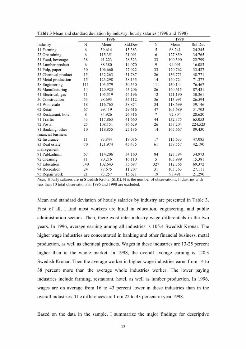
Table 3 Mean and standard deviation by industry: hourly salaries (1996 and 1998) 1996 1998 Industry N Mean Std.Dev N Mean Std.Dev 11 Farming 6 59.614 15.383 5 68.241 24.245 23 Ore mining 6 115.351 21.091 6 127.859 34.765 31 Food, beverage 38 91.223 28.523 33 100.590 22.799 33 Lumber product 6 88.380 14.070 9 94.091 16.083 34 Pulp, paper 30 106.660 27.022 33 120.762 33.427 35 Chemical product 15 132.263 51.787 26 136.771 48.771 37 Metal production 15 123.298 58.135 14 140.724 71.377 38 Engineering 111 103.579 30.530 111 130.144 76.467 39 Manufacturing 14 120.925 43.206 26 140.615 87.431 41 Electrical, gas 11 105.519 24.196 12 121.190 30.361 50 Construction 53 98.693 35.112 36 113.991 26.594 61 Wholesale 18 116.765 38.874 34 118.699 39.146 62 Retail 67 99.419 29.616 47 105.689 31.703 63 Restaurant, hotel 8 84.926 26.316 7 92.804 28.620 71 Traffic 43 117.863 41.660 44 132.375 65.053 72 Postal 25 108.151 36.629 26 157.204 224.523 81 Banking, other financial business
10 118.855 25.186 14 165.667 89.430
82 Insurance 11 93.844 19.086 17 115.633 47.085 83 Real estate management
70 121.974 45.435 61 138.557 42.190
91 Publ.admin. 67 114.206 34.160 84 123.394 34.973 92 Cleaning 11 90.216 16.110 5 103.999 15.381 93 Education 340 102.643 35.697 327 112.765 69.372 94 Recreation 24 97.675 11.207 31 103.763 27.111 95 Repair work 21 93.257 15.621 19 98.491 21.290 Note: Hourly salaries are in Swedish Krona (SEK). N is the number of observations. Industries with less than 10 total observations in 1996 and 1998 are excluded.
Mean and standard deviation of hourly salaries by industry are presented in Table 3.
First of all, I find most workers are hired in education, engineering, and public
administration sectors. Then, there exist inter-industry wage differentials in the two
years. In 1996, average earning among all industries is 105.4 Swedish Kronar. The
higher wage industries are concentrated in banking and other financial business, metal
production, as well as chemical products. Wages in these industries are 13-25 percent
higher than in the whole market. In 1998, the overall average earning is 120.3
Swedish Kronar. Then the average worker in higher wage industries earns from 14 to
38 percent more than the average whole industries worker. The lower paying
industries include farming, restaurant, hotel, as well as lumber production. In 1996,
wages are on average from 16 to 43 percent lower in these industries than in the
overall industries. The differences are from 22 to 43 percent in year 1998.
Based on the data in the sample, I summarize the major findings for descriptive
14
statistics as follows: first of all, wage dispersion exists both in 1996 and 1998, and
both average salary and the dispersion has an increased between these two years.
Second, firm size has a positive relation with wages; large firms pay higher wages
than small firms. Furthermore, there exist large wage differentials across industries as
well. However, as the sample only includes individuals who have jobs over the period
1996-1998 and other individuals are dropped, it can be expected that the average
wage and wage dispersion increase just because of the selection in our sample, such
as individuals become older and more senior during 1996-1998.

15
4. Econometric model In this section, based on the results from the descriptive statistics, I will use
econometric regression to check if the effects of firm size and industry on salaries are
statistically significant. Besides, some workers and jobs characteristics as controlling
variables will be added to the model. First, I use ordinary least square (OLS) to
estimate the wage equation as below:
𝑙𝑛𝑤𝑎𝑔𝑒!" = 𝛽! + 𝛽!𝑠𝑖𝑧𝑒!" + 𝛽!𝑖𝑛𝑑𝑢𝑠𝑡𝑟𝑦!" + 𝛽!𝐻𝐶!" + 𝛽!𝐶𝐷!" + 𝛽!𝑢𝑛𝑖𝑜𝑛!" + 𝜀!"
where 𝑙𝑛𝑤𝑎𝑔𝑒!" is log hourly wage of individual i at time t; 𝑠𝑖𝑧𝑒!" is the size
category dummy of firm j at time t; 𝑖𝑛𝑑𝑢𝑠𝑡𝑟𝑦!" is industry dummy k at time t; 𝐻𝐶!"
are human capital factors, which include schooling, age, age-square, tenure, and
tenure-square5; 𝐶𝐷!" are compensating differentials factors, which contain the job’s
hectic, monotonous, uncomfortable, noisy, dirty and overtime levels; 𝑢𝑛𝑖𝑜𝑛!" is a
union member dummy of individual i; and 𝜀!" is the error term.
As the dependent variable, wages are often used as the natural logarithm of hourly
earnings. Based on our data, the distributions of the hourly wages and its natural
logarithm form are displayed in Appendix 2. Verbeek (2008) suggests if the
dependent variable has a skewed distribution (like wages), choosing log-linear models
can suffer less from heteroskedasticity. Moreover, in order to take into account
heteroskedasticity6, I use White standard error in the model as well.
Following Edin and Zetterberg’s (1992) study in Sweden, I report the coefficients of
industry wage differentials as deviations from the employment-weighted mean
differential. It measures the wage difference between a worker in a given industry and
the average worker7. Rather than relative to the arbitrary industry group of employees,
the normalized industry wage differentials represent a more general parameterization,
5 Age-square and tenure-square are used to measure the non-linear effect of age and tenure on wage levels. 6 I use Breusch-Pagan test for heteroskedasticity. As the estimated chi-square is equal to 2456.85, this indicates a rejection of the null hypothesis that the error variances are constant. 7 Zanchi (1998) summarizes the formulation of the reported industry wage coefficient. Assume the number of industry dummies is K; (𝐾 + 1)!! is the omitted industry, it implies 𝛽!!!! = 0. 𝛽! measures the wage differential in industry k relative to (𝐾 + 1)!! industry. The employment-weighted average of wage differentials are calculated as 𝜋 = !!!!!
!!!
!. The weight is the proportion of employees belonging to this industry in the
observed sample; 𝛽! is the estimated industry coefficient. The reported industry coefficient is calculated as 𝛽!∗ = 𝛽! − 𝜋.
16
and the results are easier to interpret from the economic perspective (Zanchi, 1998).
However, the reported standard errors of the estimated parameters in Edin and
Zetterberg’s study are the unadjusted standard errors. Thus, based on the incorrect
standard errors, their results about t-test for the statistical significance of the estimated
parameters are not accurate. To fill this gap in the case of Sweden, I will use the
adjusted OLS standard errors in this study by transforming the original
variance-covariance matrix8.
As mentioned in the literature review, size-wage effects reflect differences in human
capital factors, compensating differentials, and unions between employers’ sizes.
Inter-industry wage differentials can also be determined by these factors. Therefore, I
also focus on how the differentials and effects change, once these controlling factors
are added to the model. The model is estimated four times. In model 1, the
independent variables only contain firm size, firm industry. In model 2, I include
human capital factors as control variables. In model 3, both human capital and
compensating differentials factors are added. In model 4, union dummies are included
in the model.
Besides, some studies in the literature review also assume that unobserved individual
characteristics within the error term 𝜀!" may have an influence on inter-industry
wage differentials and size-wage effects, if the error term 𝜀!" has a correlation with
observed variables, then the original OLS estimation is biased. For example, if
individuals with better unobserved personal abilities have a higher probability to be
hired in large firms, then the effect of firm size on wages will be biased upwards (Cai
and Waddoups, 2012). As our data is based on the same sample in both 1996 and
1998, then I can use the panel data fixed effects model to control for unobserved
individual characteristics. The model is presented as:
8 Following Zanchi (1998), the original variance-covariance matrix can be transformed as: 𝑣𝑎𝑟 − 𝑐𝑜𝑣 (𝛽!∗) =(𝑍 − 𝑒𝑠!)(𝑣𝑎𝑟 − 𝑐𝑜𝑣 𝛽! )(𝑍 − 𝑒𝑠!)!, where Z is a ((𝐾 + 1)×𝐾 matrix constructed as the stack of an (𝐾×𝐾) identity matrix and a (1×𝐾) row of zeros, and e is a ((𝐾 + 1)×1) vector of ones, s is the vector of employment shares of each of the first K industries. (𝑣𝑎𝑟 − 𝑐𝑜𝑣 𝛽! ) is the original variance-covariance matrix of the industry coefficients. The adjusted standard errors are the square roots of the diagonal elements of this transformed variance-covariance matrix.

17
∆𝑙𝑛𝑤𝑎𝑔𝑒!" = 𝛽! + 𝛽!∆𝑠𝑖𝑧𝑒!" + 𝛽!∆𝑖𝑛𝑑𝑢𝑠𝑡𝑟𝑦!" + 𝛽!∆𝐻𝐶!" + 𝛽!∆𝐶𝐷!"+ 𝛽!∆𝑢𝑛𝑖𝑜𝑛!" + 𝛼! + ∆𝜗!"
it shows that the error term 𝜀!" in OLS estimation is become as 𝜀!" = 𝛼! + ∆𝜗!" ,
where 𝛼! is unobserved individual fixed effects that are constant over time; and ∆𝜗!"
is the time-variant error term that is assumed to be uncorrelated with observed
variables. Since each individual is unique, it also assumes that the error term should
not be correlated with each other.
The panel data fixed effects model eliminate time-invariant individual characteristics
effects and estimate the influence of variables that vary over time. In this study, it
aims to analyze the effect on wage change over the period 1996-1998, and the effect
comes from differences within individuals. However, the original OLS estimation is
designed to measure the overall effects of industry and firm size on wage level during
1996-1998; the effects are from both changes within individuals and differences
between individuals.
An important assumption for the estimation of the fixed effects model to be unbiased
is that job change is exogenous. However, it is difficult to find a sample to avoid the
endogeneity of the job change. For example, if one industry experiences a cyclical
rise at any given time, then firms in this industry will provide higher wages and attract
mobile worker at the same time (Goux and Maurin, 1999). In order to handle with the
endogeneity of this industry change problem, it requires the identification of several
variables that are independent of the process of wage formation (Carruth et al., 2004).
However, these variables are hard to find in our dataset will lead some limitations in
the model.
18
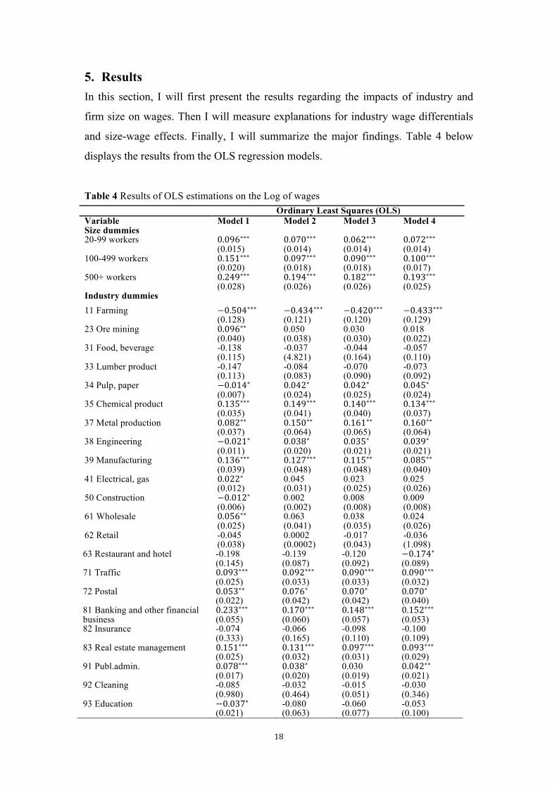
5. Results In this section, I will first present the results regarding the impacts of industry and
firm size on wages. Then I will measure explanations for industry wage differentials
and size-wage effects. Finally, I will summarize the major findings. Table 4 below
displays the results from the OLS regression models.
Table 4 Results of OLS estimations on the Log of wages Ordinary Least Squares (OLS) Variable Model 1 Model 2 Model 3 Model 4 Size dummies 20-99 workers 0.096∗∗∗
(0.015) 0.070∗∗∗ (0.014)
0.062∗∗∗ (0.014)
0.072∗∗∗ (0.014)
100-499 workers 0.151∗∗∗ (0.020)
0.097∗∗∗ (0.018)
0.090∗∗∗ (0.018)
0.100∗∗∗ (0.017)
500+ workers 0.249∗∗∗ (0.028)
0.194∗∗∗ (0.026)
0.182∗∗∗ (0.026)
0.193∗∗∗ (0.025)
Industry dummies 11 Farming −0.504∗∗∗
(0.128) −0.434∗∗∗ (0.121)
−0.420∗∗∗ (0.120)
−0.433∗∗∗ (0.129)
23 Ore mining 0.096∗∗ (0.040)
0.050 (0.038)
0.030 (0.030)
0.018 (0.022)
31 Food, beverage -0.138 (0.115)
-0.037 (4.821)
-0.044 (0.164)
-0.057 (0.110)
33 Lumber product -0.147 (0.113)
-0.084 (0.083)
-0.070 (0.090)
-0.073 (0.092)
34 Pulp, paper −0.014∗ (0.007)
0.042∗ (0.024)
0.042∗ (0.025)
0.045∗ (0.024)
35 Chemical product 0.135∗∗∗ (0.035)
0.149∗∗∗ (0.041)
0.140∗∗∗ (0.040)
0.134∗∗∗ (0.037)
37 Metal production 0.082∗∗ (0.037)
0.150∗∗ (0.064)
0.161∗∗ (0.065)
0.160∗∗ (0.064)
38 Engineering −0.021∗ (0.011)
0.038∗ (0.020)
0.035∗ (0.021)
0.039∗ (0.021)
39 Manufacturing 0.136∗∗∗ (0.039)
0.127∗∗∗ (0.048)
0.115∗∗ (0.048)
0.085∗∗ (0.040)
41 Electrical, gas 0.022∗ (0.012)
0.045 (0.031)
0.023 (0.025)
0.025 (0.026)
50 Construction −0.012∗ (0.006)
0.002 (0.002)
0.008 (0.008)
0.009 (0.008)
61 Wholesale 0.056∗∗ (0.025)
0.063 (0.041)
0.038 (0.035)
0.024 (0.026)
62 Retail -0.045 (0.038)
0.0002 (0.0002)
-0.017 (0.043)
-0.036 (1.098)
63 Restaurant and hotel -0.198 (0.145)
-0.139 (0.087)
-0.120 (0.092)
−0.174∗ (0.089)
71 Traffic 0.093∗∗∗ (0.025)
0.092∗∗∗ (0.033)
0.090∗∗∗ (0.033)
0.090∗∗∗ (0.032)
72 Postal 0.053∗∗ (0.022)
0.076∗ (0.042)
0.070∗ (0.042)
0.070∗ (0.040)
81 Banking and other financial business
0.233∗∗∗ (0.055)
0.170∗∗∗ (0.060)
0.148∗∗∗ (0.057)
0.152∗∗∗ (0.053)
82 Insurance -0.074 (0.333)
-0.066 (0.165)
-0.098 (0.110)
-0.100 (0.109)
83 Real estate management 0.151∗∗∗ (0.025)
0.131∗∗∗ (0.032)
0.097∗∗∗ (0.031)
0.093∗∗∗ (0.029)
91 Publ.admin.
0.078∗∗∗ (0.017)
0.038∗ (0.020)
0.030 (0.019)
0.042∗∗ (0.021)
92 Cleaning -0.085 (0.980)
-0.032 (0.464)
-0.015 (0.051)
-0.030 (0.346)
93 Education −0.037∗ (0.021)
-0.080 (0.063)
-0.060 (0.077)
-0.053 (0.100)
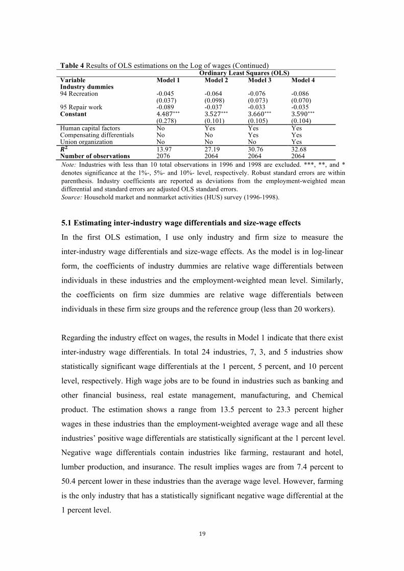
19
Table 4 Results of OLS estimations on the Log of wages (Continued) Ordinary Least Squares (OLS) Variable Model 1 Model 2 Model 3 Model 4 Industry dummies 94 Recreation -0.045
(0.037) -0.064 (0.098)
-0.076 (0.073)
-0.086 (0.070)
95 Repair work -0.089 -0.037 -0.033 -0.035 Constant 4.487∗∗∗
(0.278) 3.527∗∗∗ (0.101)
3.660∗∗∗ (0.105)
3.590∗∗∗ (0.104)
Human capital factors No Yes Yes Yes Compensating differentials No No Yes Yes Union organization No No No Yes 𝑹𝟐 13.97 27.19 30.76 32.68 Number of observations 2076 2064 2064 2064 Note: Industries with less than 10 total observations in 1996 and 1998 are excluded. ***, **, and * denotes significance at the 1%-, 5%- and 10%- level, respectively. Robust standard errors are within parenthesis. Industry coefficients are reported as deviations from the employment-weighted mean differential and standard errors are adjusted OLS standard errors. Source: Household market and nonmarket activities (HUS) survey (1996-1998).
5.1 Estimating inter-industry wage differentials and size-wage effects
In the first OLS estimation, I use only industry and firm size to measure the
inter-industry wage differentials and size-wage effects. As the model is in log-linear
form, the coefficients of industry dummies are relative wage differentials between
individuals in these industries and the employment-weighted mean level. Similarly,
the coefficients on firm size dummies are relative wage differentials between
individuals in these firm size groups and the reference group (less than 20 workers).
Regarding the industry effect on wages, the results in Model 1 indicate that there exist
inter-industry wage differentials. In total 24 industries, 7, 3, and 5 industries show
statistically significant wage differentials at the 1 percent, 5 percent, and 10 percent
level, respectively. High wage jobs are to be found in industries such as banking and
other financial business, real estate management, manufacturing, and Chemical
product. The estimation shows a range from 13.5 percent to 23.3 percent higher
wages in these industries than the employment-weighted average wage and all these
industries’ positive wage differentials are statistically significant at the 1 percent level.
Negative wage differentials contain industries like farming, restaurant and hotel,
lumber production, and insurance. The result implies wages are from 7.4 percent to
50.4 percent lower in these industries than the average wage level. However, farming
is the only industry that has a statistically significant negative wage differential at the
1 percent level.

20
Turning to size effects, the omitted size group is less than 20 workers. The results in
Model 1 show that there exists a large firm size-wage premium when the model is
estimated without any other controls. Workers in firms with 20-99 employees earn 9.6
percent higher wages than workers in firms with less than 20 employees. Similarly,
when comparing to firms with less than 20 workers, individual in firms with 100-499
workers and with 500 or more workers earn 15.1 percent and 24.9 percent more,
respectively. The firm-wage premium is monotonously increasing with firm size.
Moreover, all these positive relationships are statistically significant at the 1 percent
level. It suggests that larger firms pay substantially more to their workers than smaller
firms.
At the first sight, Model 1 suggests that there exist inter-industry wage differentials
and employer size-wage effects without other control variables; this finding is
consistent with the basic results from the descriptive statistics. Additionally, both the
effects of industry and firm size on wages are statistically significant.
5.2 Testing explanations for industry wage differentials and size-wage effects
5.2.1Human capital factors
Model 2 presents the results when human capital factors as control variables are
added. As expected, the year of schooling has a positive statistically significant
relationship to wages. Age has a positive impact on wages as well, but with age
increases, its effect on wages become increasingly smaller. Tenure unexpectedly has a
negative effect on wages. However, this relation coefficient is negligibly small. The
results of these controlling variables are reported in Appendix 3. The estimation
shows 𝑅! of the regression increases from 13.97 percent in Model 1 to 27.19 percent
in Model 2, which means human capital factors have an important influence on
wages.
For the inter-industry wage differentials, after controlling human capital factors, I find
that the numbers of wage differentials statistically significant at the 1 percent, 5
percent, and 10 percent level are reduced to 6, 1, and 4 out of 24 industries. Moreover,
the wage differentials trend to decrease in absolute size compared to model 1. For
21
example, in high-wage industries, the positive wage differentials for workers in
banking and other financial business industry of 23.3 percent are decreased to 17
percent. The negative wage differential for a worker in farming industry of -50.4
percent is reduced to -43.4 percent after including human capital factors. The results
indicate that the industry wage differentials are partly influenced by differences in
human capital factors.
Regarding the impact on size-wage effects, the first point is that the firm size effect
on wages remains statistically significant and positive once the human capital factors
are taken into account. Nevertheless, there is a reduction in the magnitude of the
effects as well. Comparing the coefficient on firm size with 500 or more workers in
Model 1 and Model 2 shows that after controlling human capital factors, workers earn
24.9 percent higher drops to 19.4 percent higher than workers in the firm with less
than 20 employees. Similarly, for workers in the firm with 100-499 employees and
20-99 workers, the positive wage differential falls by 5.4 percent and 2.6 percent,
respectively. Even including human capital factors, there exist substantial wage
differentials between large and small firms.
In sum, since the 𝑅! of the regression has a 13 percent improving compared to
Model 1, it implies that almost 13 percent of the wage differentials can be explained
by the human capital factors. Besides, the results give support for the explanation that
part of the industry wage differentials are attributed to industry differences in human
capitals. However, although these human capital factors slightly reduce the magnitude
of size wage differentials, I suggest that the human capitals have less impact on wage
differentials across firm size, as the positive statistically significance remain
unchanged.
5.2.2 Compensating differentials
Model 3 displays the results when including compensating differentials in the model.
The compensating differentials evaluate different qualities of working conditions.
Among these factors, only the influence of ‘need to work overtime at a short notice’
on wages is statistically significant. The estimation of these working conditions is
reported in Appendix 3. Compared with Model 2, the 𝑅! of the regression only
22
increases by 3 percent, which implies that these compensating differential factors
provide little additional impact on wages after controlling for human capital factors.
Comparing the coefficient on industry dummies in Model 3 with the coefficient in
Model 2 I find that including working conditions has less effect on the inter-industry
wage differentials, as the coefficients do not have substantial variation. The
compensating differentials decrease the positive wage differentials in real estate
management industry by 3.4 percent, which is the largest change in industry wage
differentials. Furthermore, the total number of wage differentials being statistically
significant remains the same. The results show that the industry wage differentials
remain almost the same when controlling for compensating differentials.
Additionally, the estimation of size-wage effects does not change so much relative to
Model 2. The coefficient on firm size with 500 or more workers shows the positive
wage differential falls by just 1.2 percent. The reductions of the differentials in firms
with 100-499 employees and 20-99 workers are even smaller. Moreover, all the
positive size wage differentials are still statistically significant at the 1 percent level
when compensating differentials are included. The results indicate that including
compensating differential variables has no impact on the size-wage effects.
In short, the 𝑅! of the regression only increases by 3 percent compared to Model 2,
which indicates that only 3 percent of the wage differentials can be attributed to the
compensating differentials after controlling human capital factors. Moreover, the
working conditions included in the regression model do not have a significant impact
on both inter-industry wage differentials and size-wage effects. The results suggest
that compensating differentials are not a key determinant of wage differentials across
industries and firm size.
5.2.3 Union organization
In Model 4, I measure if unions can provide an explanation for the inter-industry
wage differentials and firm size-wage effects. First, the degree of union membership
is displayed in Table 5 below. As expected, the union participation rates are high,
which reached nearly 90 percent both in 1996 and in 1998. However, a worker
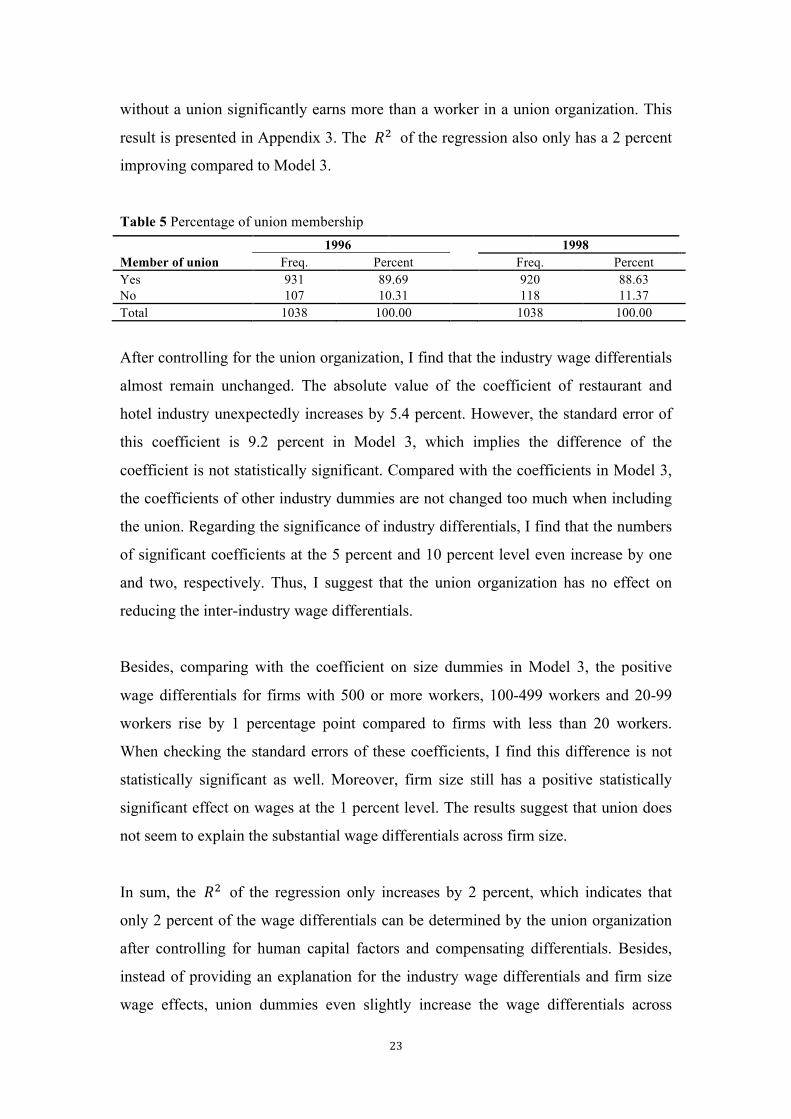
23
without a union significantly earns more than a worker in a union organization. This
result is presented in Appendix 3. The 𝑅! of the regression also only has a 2 percent
improving compared to Model 3.
Table 5 Percentage of union membership 1996 1998 Member of union Freq. Percent Freq. Percent Yes 931 89.69 920 88.63 No 107 10.31 118 11.37 Total 1038 100.00 1038 100.00 After controlling for the union organization, I find that the industry wage differentials
almost remain unchanged. The absolute value of the coefficient of restaurant and
hotel industry unexpectedly increases by 5.4 percent. However, the standard error of
this coefficient is 9.2 percent in Model 3, which implies the difference of the
coefficient is not statistically significant. Compared with the coefficients in Model 3,
the coefficients of other industry dummies are not changed too much when including
the union. Regarding the significance of industry differentials, I find that the numbers
of significant coefficients at the 5 percent and 10 percent level even increase by one
and two, respectively. Thus, I suggest that the union organization has no effect on
reducing the inter-industry wage differentials.
Besides, comparing with the coefficient on size dummies in Model 3, the positive
wage differentials for firms with 500 or more workers, 100-499 workers and 20-99
workers rise by 1 percentage point compared to firms with less than 20 workers.
When checking the standard errors of these coefficients, I find this difference is not
statistically significant as well. Moreover, firm size still has a positive statistically
significant effect on wages at the 1 percent level. The results suggest that union does
not seem to explain the substantial wage differentials across firm size.
In sum, the 𝑅! of the regression only increases by 2 percent, which indicates that
only 2 percent of the wage differentials can be determined by the union organization
after controlling for human capital factors and compensating differentials. Besides,
instead of providing an explanation for the industry wage differentials and firm size
wage effects, union dummies even slightly increase the wage differentials across
24
some industries and firm size. One expected reason is that the high degree of union
participation rates, if every worker is a union member, then union obviously has no
effect on explaining industry and size wage differentials.
5.2.4 Unobserved individual characteristics
The results presented so far suggest that inter-industry wage differentials and the
effect of firm size on wages remain when controlling for human capital factors,
compensating differentials, and union organization. As a next step, a panel data fixed
effects model is used to control for time-invariant unobserved individual
characteristics. The fixed effects model measures the effect of individuals who
changed industry or firm size on wages change over the period 1996-1998.
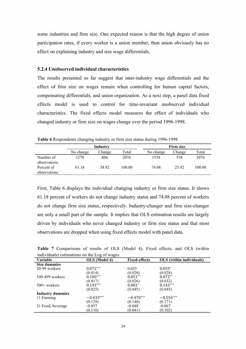
Table 6 Respondents changing industry or firm size status during 1996-1998 Industry Firm size No change Change Total No change Change Total Number of observations
1270 806 2076 1538 538 2076
Percent of observations
61.18 38.82 100.00 74.08 25.92 100.00
First, Table 6 displays the individual changing industry or firm size status. It shows
61.18 percent of workers do not change industry status and 74.08 percent of workers
do not change firm size status, respectively. Industry-changer and firm size-changer
are only a small part of the sample. It implies that OLS estimation results are largely
driven by individuals who never changed industry or firm size status and that most
observations are dropped when using fixed effects model with panel data.
Table 7 Comparisons of results of OLS (Model 4), Fixed effects, and OLS (within individuals) estimations on the Log of wages Variable OLS (Model 4) Fixed-effects OLS (within individuals) Size dummies 20-99 workers 0.072∗∗∗
(0.014) 0.025 (0.020)
0.055∗ (0.028)
100-499 workers 0.100∗∗∗ (0.017)
0.051∗∗ (0.026)
0.072∗∗ (0.032)
500+ workers 0.193∗∗∗ (0.025)
0.081∗ (0.045)
0.143∗∗∗ (0.045)
Industry dummies 11 Farming −0.433∗∗∗
(0.129) −0.470∗∗∗ (0.140)
−0.556∗∗∗ (0.171)
31 Food, beverage -0.057 (0.110)
-0.048 (0.041)
-0.067 (0.102)
25
Table 7 Comparisons of results of OLS (Model 4), Fixed effects, and OLS (within individuals) estimations on the Log of wages (Continued)Variable OLS (Model 4) Fixed-effects OLS (within individuals) Industry dummies 32 Textile −0.136∗
(0.078) 0.031 (0.079)
-0.082 (0.096)
33 Lumber product -0.073 (0.092)
0.019 (0.255)
-0.010 (0.168)
34 Pulp, paper 0.045∗ (0.024)
-0.019 (0.028)
0.002 (0.003)
35 Chemical product 0.134∗∗∗ (0.037)
0.026 (0.105)
0.069 (0.048)
37 Metal production 0.160∗∗ (0.064)
-0.052 (0.046)
-0.029 (11.873)
38 Engineering 0.039∗ (0.021)
-0.011 (0.016)
0.029 (0.024)
39 Manufacturing 0.085∗∗ (0.040)
-0.006 (0.012)
0.072∗ (0.041)
41 Electrical, gas 0.025 (0.026)
-0.036 (0.040)
-0.104 (0.147)
50 Construction 0.009 (0.008)
-0.002 (0.004)
-0.036 (0.276)
61 Wholesale 0.024 (0.026)
0.040 (0.080)
0.071∗ (0.038)
62 Retail -0.036 (1.098)
-0.016 (0.021)
-0.073 (0.083)
63 Restaurant and hotel −0.174∗ (0.089)
0.020 (0.371)
-0.076 (0.120)
71 Traffic 0.090∗∗∗ (0.032)
-0.020 (0.031)
0.018 (0.022)
72 Postal 0.070∗ (0.040)
-0.041 (0.033)
0.077∗ (0.044)
81 Banking and other financial business
0.152∗∗∗ (0.053)
0.081 (0.074)
0.178∗ (0.10)
82 Insurance -0.100 (0.109)
0.004 (0.019)
-0.018 (0.133)
83 Real estate 0.093∗∗∗ (0.029)
-0.004 (0.008)
0.050 (0.034)
91 Publ.admin.
0.042∗∗ (0.021)
0.019 (0.143)
0.014 (0.017)
92 Cleaning -0.030 (0.346)
0.048 (0.087)
-0.029 (12.828)
93 Education -0.053 (0.100)
0.015 (0.772)
0.012 (0.013)
94 Recreation -0.086 (0.070)
-0.012 (0.022)
-0.070 (0.096)
95 Repair work -0.035 0.014 -0.029 Constant 3.590∗∗∗
(0.104) 1.811∗∗ (0.848)
3.660∗∗∗ (0.105)
Human capital factors Yes Yes Yes Compensating differentials Yes Yes Yes Union Yes Yes Yes Note: Industries with less than 10 total observations in 1996 and 1998 are excluded. ***, **, and * denotes significance at the 1%-, 5%- and 10%- level, respectively. Robust standard errors are within parenthesis. Industry coefficients are reported as deviations from the employment-weighted mean differential and industry standard errors are adjusted OLS standard errors. Source: Household market and nonmarket activities (HUS) survey (1996-1998).
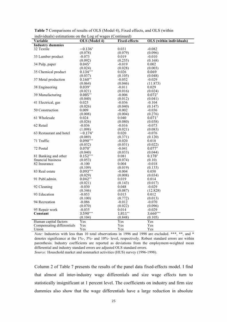
Column 2 of Table 7 presents the results of the panel data fixed-effects model. I find
that almost all inter-industry wage differentials and size wage effects turn to
statistically insignificant at 1 percent level. The coefficients on industry and firm size
dummies also show that the wage differentials have a large reduction in absolute
26
values compared to OLS Model 4. However, as shown before, most observations that
never changed industry or firm size status are deleted in the fixed effects model. It can
be expected the deviations in the results between fixed effects and OLS Model 4 may
be caused by changes in the samples. I cannot evaluate if industry wage differentials
and size-wage effects can be explained by unobserved individual characteristics
differences based on this situation.
In order to make sure the real causes of the substantial decrease in wage differentials,
I estimated the OLS Model 4 again by only including individuals who changed
industry or firm size status during 1996-1998. The comparisons of the results among
the original OLS Model 4, panel data fixed effects, and the OLS estimation focus on
differences within individuals are presented in Table 7.
When checking the industry wage differentials based on OLS estimation only
including individuals who changed industry status during 1996-1998, the results show
that most industry wage differentials change to statistically insignificant than the
original OLS Model 4, which are similar to the fixed effects model. I can expect that
the cause of change in wage differentials between fixed effects and the original OLS
Model 4 mainly due to the different samples and that unobserved individual
characteristics do not play a role in explaining industry wage differentials.
Regarding the firm size effects, the results of the OLS estimation only including
individuals who changed firm size status do not appear to be substantially different
from the original OLS Model 4. Comparing the coefficients on size dummies, the
magnitude of the positive effects from 7.2-19.3 percent higher in original OLS Model
4 falls to 5.5-14.3 percent higher than the reference group. For individuals who
changed firm size, the wage differential in firms with more than 500 workers shows
statistically significant wage differentials at the 1 percent level. However, in fixed
effects model, the firm size-wage differentials drop to only 2.5-8.1 percent, and size
wage effects turn to statistically insignificant at 1 percent level. Thus, it suggests that
size-wage effects can be partly explained by unobserved individual characteristics.
In short, the results of panel data fixed effects model show that controlling for
27
unobserved individual characteristics reduces the wage differentials substantially. For
industry wage differentials, the cause is mainly due to most observations are dropped,
and the sampling is changed. However, firm size-wage differentials can be partly
attributed to the difference in unobserved individual characteristics.
5.3 Summary
5.3.1 Inter-industry wage differentials
First of all, the results in the basic regression model indicate that industry has a
substantial effect on wages because workers in more than half of these industries have
statistically significant wage differences compared to the average worker. The high
wage industries include such as banking and other financial business, real estate
management, and manufacturing. Wages are lower in traditional industries like
farming, restaurant and hotel, lumber production. Second, when human capital factors
as control variables are added to the model, comparing the coefficients and
significance on industries dummies with the basic model the wage differentials across
industries decrease. It suggests that human capital factors seem to explain a portion of
industry wage differentials. Third, I find that compensating differentials are not an
important determinant of wage differentials across industries, as including working
condition factors does not influence the wage differentials.
Until now, I find that after controlling human capital and compensating differentials,
there are 5 and 2 industry differentials still statistically significant at 1 percent and 5
percent level, respectively. Comparing with the previous study for Sweden, Edin and
Zetterberg (1992) find that only three industry differentials are significant after
controlling for human capital factors and working condition factors. One reason is
that their study was conducted based on HUS data in 1984, and Skans et al. (2009)
suggest that there is a continuous increase in wage dispersion during 1985-2000.
Another reason may be that the reported standard errors for industry coefficients are
different in these two studies, as I calculated the adjusted OLS standard errors to get a
more consistent t-value for the statistical significance.
Then the results indicate that union has no impact on inter-industry wage differentials,
as both coefficients and significances do not change so much when adding a union

28
dummy to the model. Finally, when using panel data fixed effects model controlling
for unobserved individual characteristics; the industry wage differentials decrease
substantially and almost become statistically insignificant. However, the results based
on OLS estimation only including individuals who changed industry status show that
most industry wage differentials change to statistically insignificant as well. Thus, it
seems that the cause of change in wage differentials mainly due to the different
samples. It cannot suggest that unobserved individual characteristics could explain
industry wage differentials based on our samples.
5.3.2 Firm size-wage effects
Regarding the effect of firm size on wages, the results in the basic model show that
firm size has a positive statistically significant relationship with wages, which implies
larger firms pay higher wages than smaller firms. Moreover, the results indicate that
both human capital factors and compensating differentials provide less explanation on
size-wage effects, because even after controlling for human capital and working
condition factors, firm size still has substantial effects on wages. This finding for
Sweden is as same as the suggestion for other Europe countries, such as the study of
Schmidt and Zimmermann (1991) in Germany case.
When adding union dummies to the model, instead of reducing the wage differentials
across firm size, the estimated size-wage effects even has a slight increase. It suggests
that the wage differentials across firm size are not attributed to the high degree of
union participation in Sweden. At last, the results of the OLS estimation only
including individuals who changed firm size status do not appear to be substantially
different from the original OLS estimation. Comparing with the OLS estimation
based on individuals who changed firm size, the positive impact of firm size on wages
also decreases in the fixed effects model. The results provide support that unobserved
individual characteristics partly play a role in determining size-wage effects. This is
consistent with Cai and Waddoups’s (2012) study, who suggest that part of the effect
of firm size on wages can be explained by unobserved individual characteristics.
29
6. Concluding Remarks Wage dispersion has been shown to exist for identical workers in labor markets (Erdil
and Yetkner, 2001). This paper focuses on evaluating the effect of industry and firm
size on wages in Sweden. Both OLS regression and panel data fixed effects model are
used to measure the effects and to find determinant factors may explain inter-industry
wage differentials and size-wage effects.
In this study, the results indicate that there exist substantial wage differentials across
industries, and firm size has a positive statistically significant effect on wages.
However, human capital factors, compensating differentials, union organization, and
unobserved individual characteristics cannot fully explain the wage differentials
across industries and firm size. First, the results support the wage dispersion theory
(Mortensen, 2003), which argues that even when all employees and all employers are
identical, wage dispersion exists in labor markets and that there are inter-industry
wage differentials and size-wage effect if firms differ in productivity levels. Another
explanation for the findings is that the process of decentralized wage negotiation in
Sweden. In 1990s, the wage negotiation stronger shifted to the local enterprise level.
It would be possible that there exist wage differentials across industries and firms.
There are two limitations in this study. First, data based on the same sample are only
available in 1996 and 1998, which is short for panel method analysis. Second, some
other potential determinant factors for wage differentials across industries and firm
size are not included in our dataset, such as market power profit, the amount of
monitoring, as well as firm productivity (Weiss, 1966; Bulow and Summers, 1986;
Mortensen, 2003).
In future studies, the influences of other firm characteristics are associated with wages
can be taken into consideration in the estimations, such as ownership, occupation, and
job creation rate. In addition, the dataset that is during recent years in Sweden can be
used to measure the effect of firm characteristics on wages.
30
References Abowd, J. M., Kramarz, F. and Margolis, D. N. (1999). High wage workers and high
wage firms. Econometrica, 67, 251–333.
Akerlof, G. A. and Yellen, Y. L. (1990). The fair wage–effort hypothesis and
unemployment, Quarterly Journal of Economics, 105, 255–283.
Alback, K., Arai, M., Asplund, R., Barth, E. and Madsen, E. S. (1996). Inter-industry
wage differentials in the Nordic countries. In N. Westergård-Nielsen (Ed.). Wage
Differentials in the Nordic Countries (Part 1 of E. Waldensjö (Ed.). The Nordic
Labour Markets in the 1990’s), Elsevier, Stockholm, pp. 83–111.
Alback, K., Arai, M., Asplund, R., Barth, E. and Madsen, E. S. (1998). Measuring
wage effects of plant size. Labour Economics, 5, 425-448.
Baker, G., Jensen, M. and Murphy, K. (1988). Compensation and incentives: practice
versus theory. Journal of Finance, 43, 593–616.
Belfield, C. and Wei, X. (2004). Employer size-wage effects: evidence from matched
employer-employee survey data in the UK. Applied Economics, 36, 185–193.
Blinder, A. S. (1976). On dogmatism in human capital theory. Journal of Human
Resources, 11, 8-22.
Boeri,T. and Ours, J. V. (2013). The Economics of Imperfect Labour Markets (second
edition). Princeton University Press. Chap 8.
Brown, C. and Medoff, C. (1989). The employer size-wage effect. Journal of
Political Economy, 97, 1027-1059.
Bulow, J. and Summers, L. (1986). A Theory of Dual Labor Markets, with
Applications to Industrial Policy, Discrimination, and Keynesian Unemployment.
Journal of Labor Economics, 4, 376–414.
Cai, L-X. and Waddoups, J. (2012). Unobserved Heterogeneity, job training and the
employer size-wage effect in Australia. The Australian Economic Review,
45,158-175.
Carruth, A., Collier, W and Dickerson, A. (2004). Inter-industry wage differences and
individual heterogeneity. Oxad Bulletin of Economics and Statistics, 66 (5),
811-846.
Davis, S. J. and Haltiwanger. J. (1996). Employer size and the wage structure in the
United States. Annale d’Économie et de Statistique, 41/42, 323-368.
31
Dunne, T. and Schmitz, J. A. (1992). Wages, Employment Structure and Employer
Size-Wage Premia: Their Relationship to Advanced- Technology Usage at U.S.
Manufacturing Establishments. Discussion Paper, No. 92-15.
Edin, P-A. and Zetterberg, J. (1992). Inter-industry wage differentials: evidence from
Sweden and a comparison with the United States. American Economic Review,
82 (5), 1341-1349.
Edin, P-A. and Holmlund, B. (1995). The Swedish wage structure: the rise and fall of
solidarity wage policy? In R. B. Freeman and L. F. Katz (eds.), Differences and
changes in wage structures. University of Chicago Press, 307-344.
Erdil, E. and Yetkner, I. H. (2001). A comparative analysis of inter-industry wage
differentials: industrialized versus developing countries. Applied Economics, 33,
1639-1648.
Feldstein, M. (2008). Did wages reflect growth in productivity? Wages and
productivity.
Gao, W. and Smyth, R. (2011). Firm size and wages in China. Applied Economics
Letters, 18, 353-357.
Genre, V., Kohn, K. and Momferatou, D. (2011). Understanding inter-industry wage
structures in euro area. Applied Economics, 43, 1299-1333.
Groshen, E. L.(1991). Sources of Intra-Industry Wage Dispersion: How Much Do
Employers Matter?. Quarterly Journal of Economics, 106, 869-884.
Goux, D. and Maurin, E. (1999). The Persistence of Inter-Industry Wages
Differentials: a Reexamination on Matched Worker-firm Panel Data. Journal of
Labor Economics, 17 (3), 492-533.
Gruette, M. and Lalive, R. (2009). The importance of firms in wage determination.
Labour Economics,16, 149-160.
Hamermesh, D. S. (1993). Labor Demand Princeton. NJ: Princeton University Press.
Kramarz, F., Lollivier.S. and Pelé L-P. (1996). Wage Inequalities and Firm-Specific
Compensation Policies in France. Annale d’Économie et de Statistique, 41/42,
369-386.
Kremer, M. (1993). The O-Ring Theory of Economic Development. The Quarterly
Journal of Economics, 108, 551–575.
Krueger, A. B. and Summers, L. H. (1988). Efficiency wages and the inter-industry
wage structure. Econometrica, 56, 259–293.
32
Main, B. G. M. and Reilly, B. (1993). The employer size-wage gap: evidence for
Britain. Economica, Vo.60, 125-142.
Martins, P.S. (2007). Rent sharing and wages. Reflets et Perspectives, XLVI, 23-31.
Masters, S.H. (1969). An interindustry analysis of wages and plant size. The Review
of Economics and Statistics, Vol.51, 3, 341-345.
Mcconnell,C.R., Brue, S.L. and Macpherson, D. (2009). Contemporary Labor
Economics. McGraw-Hill Education.
Mincer, J. (1974). Schooling, experience, and earnings. New York: Columbia
University Press.
Morissette, R. (1993). Canadian jobs and firm size: Do smaller firms pay less?. The
Canadian Journal of Economics, 26,159-174.
Mortensen, D. T. (2003). Wage Dispersion: Why Are Similar Workers Paid
Differently?. Cambridge, MA: MIT press.
Naylor, R. (2003). Economic models of union behavior. In J. T. Addison and C.
Schnabel (eds.), International Handbook of Trade Unions. Edward Elgar,
Cheltenham and Northampton, 44–85.
Oi, W. Y. (1983). The Fixed Employment Costs of Specialized Labor. In Jack E.
Triplett (eds.), The Measurement of Labor Costs . Chicago: University of
Chicago Press for NBER.�
Oi, W. Y. and Idson, T. L. (1999). Firm size and wages. In O. Ashenfelter and D.
Card, (eds.). Handbook of Labour Economics, Vol. 3B. Amsterdam: Elsevier,
2165–2214.
Purse, K. (2004). Work-related fatality risks and neoclassical compensating wage
differentials. Cambridge Journal of Economics, 28, 597–617.
Rosen, S. (1986). The Theory of Equalizing Differences. In O. Ashenfelter and R.
Layard, (eds.).Handbook of Labor Economics, Vol 1. Elsevier. 641-692.
Schmidt, C. M. and Zimmermann, K. F. (1991). Work Characteristics, Firm Size and
Wages. The Review of Economics and Statistics, 73, 705–710.
Skans, O.N., Edin, P-A. and Holmlund, B. (2009). Wage dispersion between and
within plants: Sweden 1985-2000. In E. P. Lazear and K. L. Shaw (eds.),
National Bureau of economic research comparative labor markets series: the
structure of wages: an international comparison. University of Chicago Press,
217-20.
33
Topel, R. H.and Ward, M. P. (1992). Job Mobility and the Careers of Young Men.
Quarterly Journal of Economics, 107, 439- 479.
Troske, K. R. (1999). Evidence on the employer size–wage premium from
worker-establishment matched data. The Review of Economics and Statistics, 81
(1), 15–26.
Vainiomäki, J. and Laaksonen, S. (1995). Inter-industry wage differentials in Finland:
Evidence form longitudinal census data for 1975-85. Labour Economics, 2,
161-173.
Verbeek, M. (2008). Guide to Modern Econometrics. 3rd ed. West Sussex: John
Wiley & Sons Ltd.
Waddoups, C. J. (2007). Employer size–wage effects in Australia. LABOUR: Review
of Labour Economics and Industrial Relations, 21, 809–35.
Wagner, J. (1997). Firm size and job quality. A survey of the evidence from Germany,
Small Business Economics, 9, 411–25.
Weiss, L. (1966). Concentration and Labor Earnings. American Economic Review
56, 96–117.
Zanchi, L. (1998). Interindustry wage differentials in dummy variable models.
Economics Letters, 60, 297-301.
34
Appendix
Appendix 1: The description of the control variables
Human capital factors:
School years: years of schools and vocational training.
Age: calculated as the difference between the survey year and the birth year.
Tenure: calculated as the difference between the survey year and the hired year of
current job.
Compensating differentials:
These variables are based on some questions to the employees about their work
environment.
Hectic: is your job hectic?
1 if often, 2 if sometimes, 3 if rarely or never.
Monotonous: is your job monotonous?
1 if often, 2 if sometimes, 3 if rarely or never.
Uncomfortable: is your work such that you need to assume bent over, twisted or other
uncomfortable positions?
1 if often, 2 if sometimes, 3 if rarely or never.
Noisy: is it noisy were you work?
1 if often, 2 if sometimes, 3 if rarely or never.
Dirty: do you get dirty when you are working?
1 if often, 2 if sometimes, 3 if rarely or never.
Overtime: are you able to determine for yourself how to do your job?
1 if often, 2 if sometimes, 3 if rarely or never.
Union member: are you a member of a union?
1 if yes, 2 if no.
Source: Household market and nonmarket activities (HUS) survey (1996-1998).

35
Appendix 2: Distribution of the dependent variable
Figure 1 Histogram of the hourly wages with normal density
Figure 2 Histogram of the natural logarithm of hourly wages with normal density

36
Appendix 3: Results of control variables on the log of wages in Table 4 Variable Model 2 Model 3 Model 4 Human capitals School years 0.033∗∗∗
(0.002) 0.027∗∗∗ (0.002)
0.027∗∗∗ (0.002)
Age 0.022∗∗∗ (0.004)
0.018∗∗∗ (0.004)
0.020∗∗∗ (0.004)
Age-square −0.0001∗∗∗ (0.00005)
−0.0001∗∗∗ (0.00005)
−0.0001∗∗∗ (0.00005)
Tenure −0.003∗ (0.0020)
-0.002 (0.0020)
-0.0009 (0.0020)
Tenure-square 0.0001∗∗ (0.00005)
0.00009∗ (0.00005)
-0.00006 (0.00005)
Compensating differentials Hectic
Sometimes
-0.019 (0.013)
−0.023∗ (0.013)
Rarely or never
-0.036 (0.026)
-0.040 (0.026)
Monotonous Sometimes
0.036 (0.029)
0.036 (0.029)
Rarely or never
0.042 (0.027)
0.039 (0.028)
Uncomfortable Sometimes
0.026 (0.017)
0.027∗ (0.017)
Rarely or never
0.117∗∗∗ (0.018)
0.113∗∗∗ (0.018)
Noisy Sometimes
-0.014 (0.020)
-0.008 (0.020)
Rarely or never
0.031∗ (0.018)
0.027 (0.018)
Dirty Sometimes
-0.021 (0.020)
-0.023 (0.020)
Rarely or never
-0.023 (0.020)
-0.034 (0.020)
Overtime Sometimes
−0.037∗∗ (0.017)
−0.027∗ (0.016)
Rarely or never
−0.056∗∗∗ (0.018)
−0.047∗∗ (0.017)
Union member No
0.156∗∗∗ (0.024)
Note: ***, **, and * denotes significance at the 1%-, 5%- and 10%- level, respectively. Robust standard errors are within parenthesis. For compensating differentials factors, the reference group answer is “often”. For Union member, the reference group is “Yes”. Source: Household market and nonmarket activities (HUS) survey (1996-1998).