Firm Characteristics and Chinese Stocks

JMSE 2018, 3(4), 259–283 http://www.jmse.org.cn/doi:10.3724/SP.J.1383.304014 http://engine.scichina.com/publisher/CSPM/journal/JMSE

Article

Firm Characteristics and Chinese Stocks

Fuwei Jiang 1, Guohao Tang 2,* and Guofu Zhou 3,4

1 School of Finance, Central University of Finance and Economics, Beijing 100081, China; [email protected] College of Finance and Statistics, Hunan University, Changsha 410006, China3 Olin Business School, Washington University in St. Louis, St. Louis, MO 63130, USA; [email protected] China Academy of Financial Research, Shanghai Advanced Institute of Finance, Shanghai 200000, China

* Correspondence: [email protected]

Received: 31 May 2018; Accepted: 26 November 2018; Published: 22 February 2019

Abstract: This paper presents a comprehensive study on predicting the cross section of Chinese stock marketreturns with a large panel of 75 individual firm characteristics. We use not only the traditional Fama-MacBethregression, but also the “big-data” econometric methods: principal component analysis (PCA), partial leastsquares (PLS), and forecast combination to extract information from all the 75 firm characteristics. Thesecharacteristics are important return predictors, with statistical and economic significance. Furthermore, firmcharacteristics that are related to trading frictions, momentum, and profitability are the most effective predictorsof future stock returns in the Chinese stock market.

Keywords: Partial least squares; Machine learning; Firm characteristics; Chinese stock market; Returnpredictability

1. Introduction

A fundamental problem in finance is explaining why different assets deliver different returns. In the USmarket, a large number of studies document dozens of firm characteristics that forecast the cross section of stockreturns (Goyal, 2012; Harvey et al., 2016; McLean and Pontiff, 2016). For example, Green et al. (2017) and Hanet al. (2018) examine the predictive power of 94 firm characteristics. Yan and Zheng (2017) use the bootstrapapproach to construct thousands of fundamental signals from financial statements to predict cross-sectionalreturns. In his AFA 2011 Presidential Address, John Cochrane refers to the proposed anomalies as “a zoo of newvariables” and argues that researchers should use novel econometric methods to synthesize the huge amount ofreturn predictors documented in the previous studies.

In this study, we take up the challenge raised by Cochrane regarding the Chinese stock market. We create alarge comprehensive set of 75 firm characteristics that are known to be related to expected returns from the mostrecent anomalies literature and examine their individual economic relevance and predictive power. We then

259

Downloaded to IP: 192.168.0.24 On: 2019-03-12 04:11:11 http://engine.scichina.com/doi/10.3724/SP.J.1383.304014

260 JMSE 2018, 3(4), 259–283

study the information contained in all of the 75 firm characteristics on predicting the cross-sectional Chinesestock market returns. Since it is impossible to know, ex ante, which firm characteristics will have the greatestpredictive ability in the future, it is important to examine all of them collectively, so that the forecasting strategyis implementable in real time.

In aggregating the information of all firm characteristics, we use not only the traditional Fama-MacBethregression, but also the “big-data” econometric methods, including the principal component analysis (PCA),forecast combination (FC), and partial least squares (PLS) methods. PCA is a widely used dimension reductiontool, but it best explains the variance of the characteristics and not necessarily the asset returns. The FC methodis the average of univariate regressions on each firm characteristic. While the combination method has a longhistory in economics (Timmermann, 2006), the FC method is used primarily in time series forecasting. Here, weapply the technique in the cross section similar to Han et al. (2018). The PLS method, developed recently byLight et al. (2017), extracts information from the characteristics to have the greatest covariance with the returns.Based on these methods, we synthesize information from all firm characteristics, construct pricing factors, andform decile portfolios accordingly. We calculate the long-short portfolios’ returns, Sharpe ratios, and abnormalreturns to evaluate the effectiveness of the four estimation techniques.

The univariate portfolio analysis shows that 18 out of 75 firm characteristics produce statistically significantvalue-weighted long-short spread portfolio returns at the 10% level, 15 of them are significant at the 5% level,and 8 of them are significant at the 1% level. Interestingly, unlike in the US market, size has the highestvalue-weighted monthly hedge return of 1.84% (t = 3.39), while the highest value-weighted Fama-Frenchfive-factor (FF5) alpha is generated by return on assets (ROA) at 1.46% (t = 5.95) per month.

All of the four aggregation methods except PCA show joint return predictive power and PLS performsbest. Specifically, we form ten decile portfolios according to the latent factor estimated using the PLS methodand find that the decile portfolio returns increase monotonically with the PLS factor, and the long-short spreadportfolio on the PLS factor generates sizable monthly average returns of 2.60% and 1.95% with the t-statistics5.98 and 4.07 for equal- and value-weighting schemes, respectively. In addition, the spread portfolio return ofthe PLS factor model is larger than all the sorted portfolio returns by individual firm characteristics, indicatingstrong economic gain from information aggregation.

We also test whether the PLS factor can be explained by the FF5 models (Fama and French, 2015), addingto the extensive literature on which anomalies in the stock market can be explained by the five factors, whichare the market, size, value, profitability, or investment. Our results indicate that the PLS-based approach hassignificant FF5 alphas, implying that the PLS technique can extract a common factor with additional forecastinginformation for the Chinese market than the FF5 model. Moreover, the Sharpe ratios of the PLS long-shortportfolios are high, ranging from 1.48 to 1.66 for equal-weighted portfolios and 0.81 to 1.03 for value-weightedportfolios.

In comparison, the PCA method generates insignificant spread portfolio return, suggesting that a largepart of the common variation in firm characteristics are common noises that are unrelated to expected stockreturns. In addition, the Fama-MacBeth (FM) regression and the FC method are less informative than PLS. Thevalue-weighted monthly hedge return of the FM factor portfolio is 1.01% (t = 2.61), while the value-weightedFC factor spread portfolio return is 0.74% (t = 1.60) per month.

Moreover, we cluster and classify these 75 characteristics into six categories comprising thevalue-versus-growth, investment, profitability, momentum, trading frictions, and intangibles groups. By


JMSE 2018, 3(4), 259–283 261

employing the PLS approach, we find that variables belonging to trading frictions, momentum, and profitabilityare more effective in forecasting cross-sectional expected returns in the Chinese stock market. For example, thetrading friction-based PLS factor spread portfolios generate 2.24% (t = 5.47) and 1.86% (t = 4.23) equal- andvalue-weighted monthly returns, respectively.

Our study contributes to the growing asset-pricing literature on the Chinese stock market, which hasgrown rapidly over time and now ranks the second largest in the world, becoming an increasingly importantpart of the global capital market. Carpenter et al. (2015) find that the informativeness of the Chinese markethas recently increased significantly. Jiang et al. (2011) conduct a comprehensive investigation of the time-seriesreturn predictability of the Chinese stock market with many predictor variables. Jiang et al. (2018) study thecross-sectional predictability of the Chinese stock market with only three profitability variables. However, thereare no mega studies on the cross-sectional predictability of the Chinese stock market. In contrast, we conduct,by far, the most comprehensive study of the cross-sectional return predictability of the Chinese stock marketwith 75 accounting- and return-related firm characteristics.

Our study also contributes to the asset pricing literature on firm characteristics that forecast a cross sectionof stock returns. Stambaugh et al. (2012) show that investor sentiment contributes to the predictive power of11 anomalies. Novy-Marx and Velikov (2015) investigate the after-trading cost performance of 23 anomalies.McLean and Pontiff (2016) examine the post-publication return predictability on 97 anomalies. Hou et al. (2017)replicate 447 anomalies in the finance and accounting literature. Han et al. (2018) provide a portfolio rebalancingstrategy to enhance anomaly performance. We extend the literature and conduct the first comprehensive studyin assessing the return predictive power of a large number of firm characteristics in the Chinese market.

Our paper is also closely related to the growing works on applying machine learning and big datatechniques in the financial market. Gu et al. (2018), Han et al. (2018) and Jiang et al. (2019) apply a numberof machine learning tools to finance. But our current paper focus on using PCA, FC and PLS. Light et al.(2017) propose the PLS approach for estimating expected returns on individual stocks from cross-sectionalfirm characteristics. Their econometric method is related to the time series PLS adopted by Kelly and Pruitt(2013, 2015), Huang et al. (2015), and Jiang et al. (2018). Based on the Welch and Goyal (2008) predictor dataset,Rapach et al. (2010) show that combination is a powerful forecasting method for the time series of stock returnswith a shrinkage interpretation, and Neely et al. (2014) propose the PCA approach to forecast aggregate USstock returns. We conduct a comparative analysis on different machine learning techniques in forecasting thecross-sectional expected stock returns in the Chinese market setting.

The remainder of this paper is organized as follows. Section 2 discusses the data and calculation of 75anomalies. Section 3 explores the univariate portfolio analysis of individual firm characteristics. Section 4employs portfolio tests to compare various information aggregation methods and investigates the returnpredictability for different categories of firm characteristics. Section 5 concludes the paper.

2. Data

We obtain the data from the China Stock Market & Accounting Research (CSMAR) spanning January 1998to December 2016, including accounting data, monthly stock returns, Fama-French common factors (1993, 2015),and Chinese risk-free rates. Following Allen et al. (2015) and Carpenter et al. (2015), our sample consisted of


262 JMSE 2018, 3(4), 259–283

all Chinese A-share stocks with accounting and returns data available. Stocks are traded on the Shanghai andShenzhen main boards, SME Board, and ChiNext Board, to cover different levels of Chinese stock markets.

To ensure the quality of data, we applied standard sample screening procedures. First, we excluded firmquarterly observations with “ST” (special treatment) and/or “PT” (particular transfer) status at the beginning ofportfolio formation, which are stocks under financial distress and lack market liquidity. According to Allen etal. (2015) and Carpenter et al. (2015), “ST” and “PT” firms are usually under financial distress, illiquid, and atthe risk of delisting. In the Chinese stock market, common stocks have a daily price up/down limit of 10%.However, the daily limit for “ST” and “PT” stocks is only 5%. In unreported tables, we find similar results whenincluding “ST” and “PT” stocks. Second, we excluded firms in the financial industry according to the industryclassification of the China Securities Regulatory Commission (CSRC). According to Fama and French (1992),financial firms typically have much higher leverage ratios than non-financial firms, for which high leverageusually indicates distress. In unreported tables, we find similar results when including financial firms.

We use the sample period from 2000 to 2016 in our main tests, after China’s entry into the World TradeOrganization (WTO). According to Carpenter et al. (2015), a series of reforms and developments, such as theinitiation of securities laws and regulations, were introduced by the CSRC authority during this period toincrease Chinese stock market transparency, audit quality, protection of minority shareholders, and generalfunctioning and efficiency.

As fundamental signals for expected stock returns, we use 75 variables derived from well-known, recentasset-pricing literature. These firm-level characteristics can be classified into six categories. The first categoryincludes value-versus-growth-related variables, such as asset-to-market (AM), book-to-market equity (BM),cash flow-to-price (CFP), debt-to-equity ratio (DER), earnings-to-price (EP), and sales-to-price (SP). The secondcategory contains investment-based characteristics such as accruals (ACC), capital expenditure growth (CAPXG),change in shareholders’ equity (dBe), investment-to-assets (IA), inventory change (IVC), and net operatingassets (NOA). The third group contains profitability-related variables such as asset turnover (ATO), cashproductivity (CP), earnings before interest and taxes (EBIT), gross profitability (GP), return on assets (ROA),and return on equity (ROE). The fourth category includes momentum-related variables such as change in6-month momentum (CHMOM), industry momentum (INMOM), 1-month momentum (MOM1M), 12-monthmomentum (MOM12M), volume momentum (VOLM), and volume trend (VOLT). The fifth group containstrading frictions-related characteristics such as market beta (BETA), idiosyncratic return volatility (IVOL),illiquidity (ILLIQ), price (PRC), firm size (SIZE), and share turnover (TURN). The last category includesintangibles-related variables such as firm age (AGE), cash flow-to-debt (CFD), current ratio (CR), quick ratio(QR), sales-to-cash (SC), and sales-to-inventory (SI). The definition of each variable is described in Appendix Band largely follows the original paper in which the variable is calculated and constructed as related to stockreturns.

3. Univariate portfolio analysis on individual characteristics

We start our empirical study by investigating whether the firm individual characteristics can separatelypredict cross-sectional stock returns. We sort all stocks with respect to each characteristic depending on datafrequency. For most characteristics from the firm’s fiscal year report, we form 10 decile portfolios at the endof June of year t according to the ranked values of each firm characteristic for the fiscal year ending in year


JMSE 2018, 3(4), 259–283 263

t-1. Following Jiang et al. (2018), the portfolios based on gross profitability (GP), return on assets (ROA), andreturn on equity (ROE) use quarterly accounting data. These portfolios and other return-related portfolios, suchas momentum, size, beta, and volatility are rebalanced at the end of each month by using the most recentlyavailable data. We then calculate monthly equal- and value-weighted returns on them. The return predictabilityof each characteristic is the difference between the realized return on top and bottom decile portfolios, which isreferred to as the long-short portfolio returns. We invert the long and short portfolios if the characteristics arenegatively related to future returns.

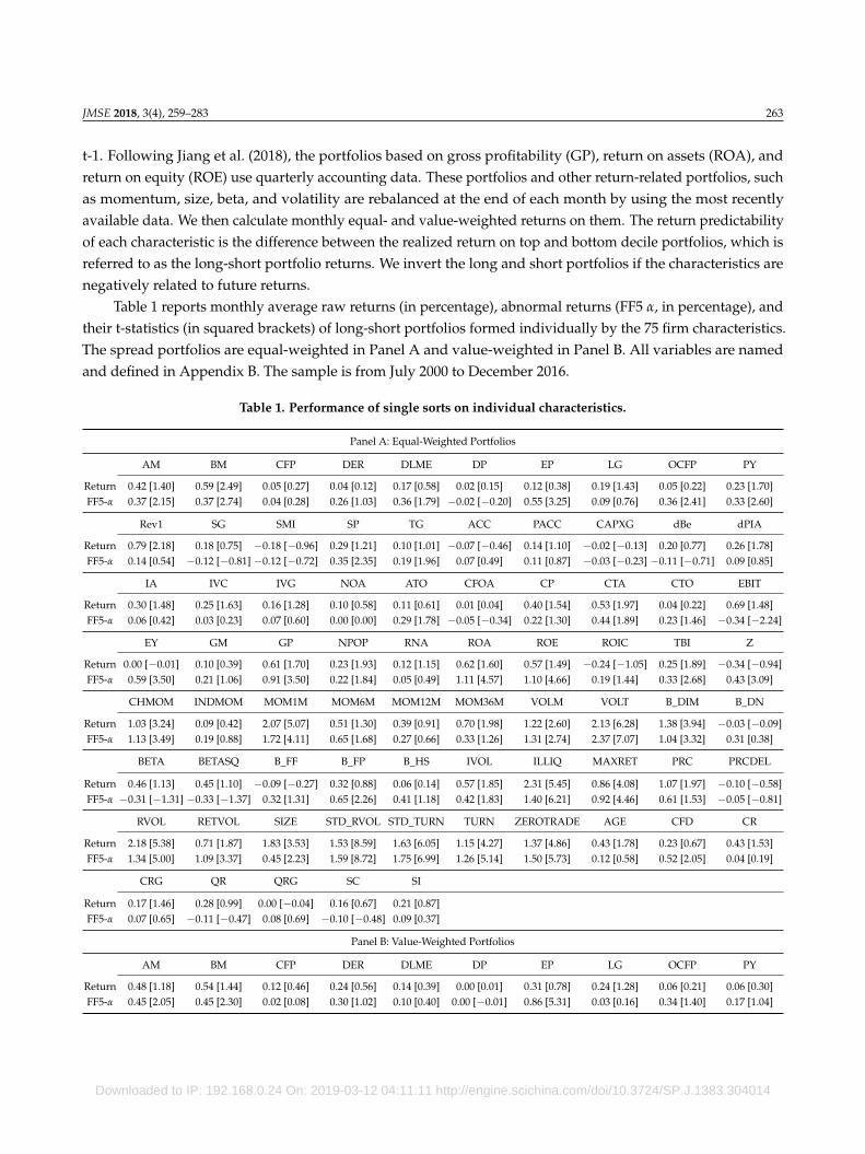
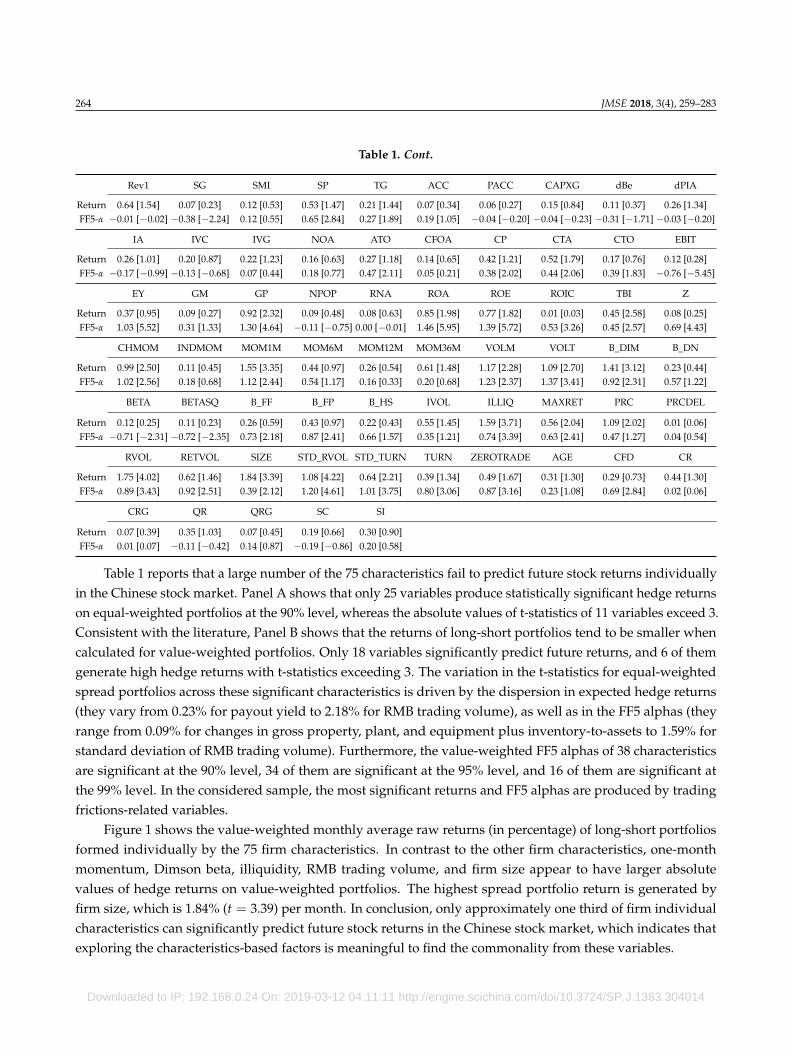
Table 1 reports monthly average raw returns (in percentage), abnormal returns (FF5 α, in percentage), andtheir t-statistics (in squared brackets) of long-short portfolios formed individually by the 75 firm characteristics.The spread portfolios are equal-weighted in Panel A and value-weighted in Panel B. All variables are namedand defined in Appendix B. The sample is from July 2000 to December 2016.

Table 1. Performance of single sorts on individual characteristics.

Panel A: Equal-Weighted Portfolios

AM BM CFP DER DLME DP EP LG OCFP PY

Return 0.42 [1.40] 0.59 [2.49] 0.05 [0.27] 0.04 [0.12] 0.17 [0.58] 0.02 [0.15] 0.12 [0.38] 0.19 [1.43] 0.05 [0.22] 0.23 [1.70]FF5-α 0.37 [2.15] 0.37 [2.74] 0.04 [0.28] 0.26 [1.03] 0.36 [1.79] −0.02 [−0.20] 0.55 [3.25] 0.09 [0.76] 0.36 [2.41] 0.33 [2.60]

Rev1 SG SMI SP TG ACC PACC CAPXG dBe dPIA

Return 0.79 [2.18] 0.18 [0.75] −0.18 [−0.96] 0.29 [1.21] 0.10 [1.01] −0.07 [−0.46] 0.14 [1.10] −0.02 [−0.13] 0.20 [0.77] 0.26 [1.78]FF5-α 0.14 [0.54] −0.12 [−0.81] −0.12 [−0.72] 0.35 [2.35] 0.19 [1.96] 0.07 [0.49] 0.11 [0.87] −0.03 [−0.23] −0.11 [−0.71] 0.09 [0.85]

IA IVC IVG NOA ATO CFOA CP CTA CTO EBIT

Return 0.30 [1.48] 0.25 [1.63] 0.16 [1.28] 0.10 [0.58] 0.11 [0.61] 0.01 [0.04] 0.40 [1.54] 0.53 [1.97] 0.04 [0.22] 0.69 [1.48]FF5-α 0.06 [0.42] 0.03 [0.23] 0.07 [0.60] 0.00 [0.00] 0.29 [1.78] −0.05 [−0.34] 0.22 [1.30] 0.44 [1.89] 0.23 [1.46] −0.34 [−2.24]

EY GM GP NPOP RNA ROA ROE ROIC TBI Z

Return 0.00 [−0.01] 0.10 [0.39] 0.61 [1.70] 0.23 [1.93] 0.12 [1.15] 0.62 [1.60] 0.57 [1.49] −0.24 [−1.05] 0.25 [1.89] −0.34 [−0.94]FF5-α 0.59 [3.50] 0.21 [1.06] 0.91 [3.50] 0.22 [1.84] 0.05 [0.49] 1.11 [4.57] 1.10 [4.66] 0.19 [1.44] 0.33 [2.68] 0.43 [3.09]

CHMOM INDMOM MOM1M MOM6M MOM12M MOM36M VOLM VOLT B_DIM B_DN

Return 1.03 [3.24] 0.09 [0.42] 2.07 [5.07] 0.51 [1.30] 0.39 [0.91] 0.70 [1.98] 1.22 [2.60] 2.13 [6.28] 1.38 [3.94] −0.03 [−0.09]FF5-α 1.13 [3.49] 0.19 [0.88] 1.72 [4.11] 0.65 [1.68] 0.27 [0.66] 0.33 [1.26] 1.31 [2.74] 2.37 [7.07] 1.04 [3.32] 0.31 [0.38]

BETA BETASQ B_FF B_FP B_HS IVOL ILLIQ MAXRET PRC PRCDEL

Return 0.46 [1.13] 0.45 [1.10] −0.09 [−0.27] 0.32 [0.88] 0.06 [0.14] 0.57 [1.85] 2.31 [5.45] 0.86 [4.08] 1.07 [1.97] −0.10 [−0.58]FF5-α −0.31 [−1.31] −0.33 [−1.37] 0.32 [1.31] 0.65 [2.26] 0.41 [1.18] 0.42 [1.83] 1.40 [6.21] 0.92 [4.46] 0.61 [1.53] −0.05 [−0.81]

RVOL RETVOL SIZE STD_RVOL STD_TURN TURN ZEROTRADE AGE CFD CR

Return 2.18 [5.38] 0.71 [1.87] 1.83 [3.53] 1.53 [8.59] 1.63 [6.05] 1.15 [4.27] 1.37 [4.86] 0.43 [1.78] 0.23 [0.67] 0.43 [1.53]FF5-α 1.34 [5.00] 1.09 [3.37] 0.45 [2.23] 1.59 [8.72] 1.75 [6.99] 1.26 [5.14] 1.50 [5.73] 0.12 [0.58] 0.52 [2.05] 0.04 [0.19]

CRG QR QRG SC SI

Return 0.17 [1.46] 0.28 [0.99] 0.00 [−0.04] 0.16 [0.67] 0.21 [0.87]FF5-α 0.07 [0.65] −0.11 [−0.47] 0.08 [0.69] −0.10 [−0.48] 0.09 [0.37]

Panel B: Value-Weighted Portfolios

AM BM CFP DER DLME DP EP LG OCFP PY

Return 0.48 [1.18] 0.54 [1.44] 0.12 [0.46] 0.24 [0.56] 0.14 [0.39] 0.00 [0.01] 0.31 [0.78] 0.24 [1.28] 0.06 [0.21] 0.06 [0.30]FF5-α 0.45 [2.05] 0.45 [2.30] 0.02 [0.08] 0.30 [1.02] 0.10 [0.40] 0.00 [−0.01] 0.86 [5.31] 0.03 [0.16] 0.34 [1.40] 0.17 [1.04]


264 JMSE 2018, 3(4), 259–283

Table 1. Cont.

Rev1 SG SMI SP TG ACC PACC CAPXG dBe dPIA

Return 0.64 [1.54] 0.07 [0.23] 0.12 [0.53] 0.53 [1.47] 0.21 [1.44] 0.07 [0.34] 0.06 [0.27] 0.15 [0.84] 0.11 [0.37] 0.26 [1.34]FF5-α −0.01 [−0.02] −0.38 [−2.24] 0.12 [0.55] 0.65 [2.84] 0.27 [1.89] 0.19 [1.05] −0.04 [−0.20] −0.04 [−0.23] −0.31 [−1.71] −0.03 [−0.20]

IA IVC IVG NOA ATO CFOA CP CTA CTO EBIT

Return 0.26 [1.01] 0.20 [0.87] 0.22 [1.23] 0.16 [0.63] 0.27 [1.18] 0.14 [0.65] 0.42 [1.21] 0.52 [1.79] 0.17 [0.76] 0.12 [0.28]FF5-α −0.17 [−0.99] −0.13 [−0.68] 0.07 [0.44] 0.18 [0.77] 0.47 [2.11] 0.05 [0.21] 0.38 [2.02] 0.44 [2.06] 0.39 [1.83] −0.76 [−5.45]

EY GM GP NPOP RNA ROA ROE ROIC TBI Z

Return 0.37 [0.95] 0.09 [0.27] 0.92 [2.32] 0.09 [0.48] 0.08 [0.63] 0.85 [1.98] 0.77 [1.82] 0.01 [0.03] 0.45 [2.58] 0.08 [0.25]FF5-α 1.03 [5.52] 0.31 [1.33] 1.30 [4.64] −0.11 [−0.75] 0.00 [−0.01] 1.46 [5.95] 1.39 [5.72] 0.53 [3.26] 0.45 [2.57] 0.69 [4.43]

CHMOM INDMOM MOM1M MOM6M MOM12M MOM36M VOLM VOLT B_DIM B_DN

Return 0.99 [2.50] 0.11 [0.45] 1.55 [3.35] 0.44 [0.97] 0.26 [0.54] 0.61 [1.48] 1.17 [2.28] 1.09 [2.70] 1.41 [3.12] 0.23 [0.44]FF5-α 1.02 [2.56] 0.18 [0.68] 1.12 [2.44] 0.54 [1.17] 0.16 [0.33] 0.20 [0.68] 1.23 [2.37] 1.37 [3.41] 0.92 [2.31] 0.57 [1.22]

BETA BETASQ B_FF B_FP B_HS IVOL ILLIQ MAXRET PRC PRCDEL

Return 0.12 [0.25] 0.11 [0.23] 0.26 [0.59] 0.43 [0.97] 0.22 [0.43] 0.55 [1.45] 1.59 [3.71] 0.56 [2.04] 1.09 [2.02] 0.01 [0.06]FF5-α −0.71 [−2.31] −0.72 [−2.35] 0.73 [2.18] 0.87 [2.41] 0.66 [1.57] 0.35 [1.21] 0.74 [3.39] 0.63 [2.41] 0.47 [1.27] 0.04 [0.54]

RVOL RETVOL SIZE STD_RVOL STD_TURN TURN ZEROTRADE AGE CFD CR

Return 1.75 [4.02] 0.62 [1.46] 1.84 [3.39] 1.08 [4.22] 0.64 [2.21] 0.39 [1.34] 0.49 [1.67] 0.31 [1.30] 0.29 [0.73] 0.44 [1.30]FF5-α 0.89 [3.43] 0.92 [2.51] 0.39 [2.12] 1.20 [4.61] 1.01 [3.75] 0.80 [3.06] 0.87 [3.16] 0.23 [1.08] 0.69 [2.84] 0.02 [0.06]

CRG QR QRG SC SI

Return 0.07 [0.39] 0.35 [1.03] 0.07 [0.45] 0.19 [0.66] 0.30 [0.90]FF5-α 0.01 [0.07] −0.11 [−0.42] 0.14 [0.87] −0.19 [−0.86] 0.20 [0.58]

Table 1 reports that a large number of the 75 characteristics fail to predict future stock returns individuallyin the Chinese stock market. Panel A shows that only 25 variables produce statistically significant hedge returnson equal-weighted portfolios at the 90% level, whereas the absolute values of t-statistics of 11 variables exceed 3.Consistent with the literature, Panel B shows that the returns of long-short portfolios tend to be smaller whencalculated for value-weighted portfolios. Only 18 variables significantly predict future returns, and 6 of themgenerate high hedge returns with t-statistics exceeding 3. The variation in the t-statistics for equal-weightedspread portfolios across these significant characteristics is driven by the dispersion in expected hedge returns(they vary from 0.23% for payout yield to 2.18% for RMB trading volume), as well as in the FF5 alphas (theyrange from 0.09% for changes in gross property, plant, and equipment plus inventory-to-assets to 1.59% forstandard deviation of RMB trading volume). Furthermore, the value-weighted FF5 alphas of 38 characteristicsare significant at the 90% level, 34 of them are significant at the 95% level, and 16 of them are significant atthe 99% level. In the considered sample, the most significant returns and FF5 alphas are produced by tradingfrictions-related variables.

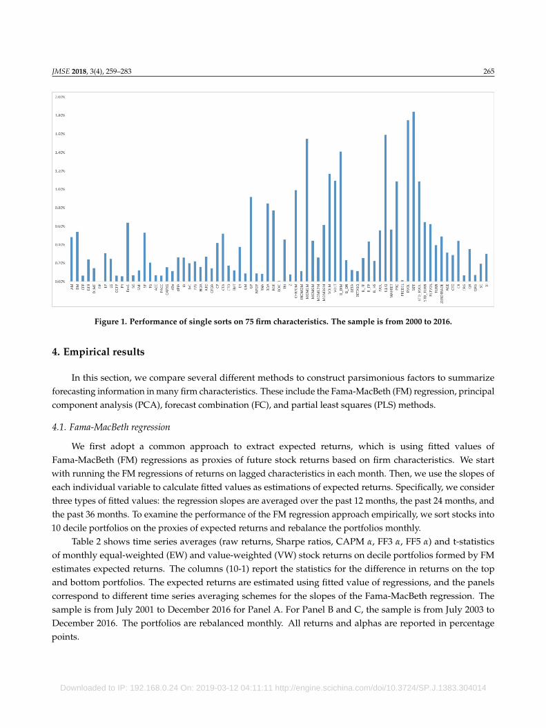
Figure 1 shows the value-weighted monthly average raw returns (in percentage) of long-short portfoliosformed individually by the 75 firm characteristics. In contrast to the other firm characteristics, one-monthmomentum, Dimson beta, illiquidity, RMB trading volume, and firm size appear to have larger absolutevalues of hedge returns on value-weighted portfolios. The highest spread portfolio return is generated byfirm size, which is 1.84% (t = 3.39) per month. In conclusion, only approximately one third of firm individualcharacteristics can significantly predict future stock returns in the Chinese stock market, which indicates thatexploring the characteristics-based factors is meaningful to find the commonality from these variables.


JMSE 2018, 3(4), 259–283 265

Figure 1. Performance of single sorts on 75 firm characteristics. The sample is from 2000 to 2016.

4. Empirical results

In this section, we compare several different methods to construct parsimonious factors to summarizeforecasting information in many firm characteristics. These include the Fama-MacBeth (FM) regression, principalcomponent analysis (PCA), forecast combination (FC), and partial least squares (PLS) methods.

4.1. Fama-MacBeth regression

We first adopt a common approach to extract expected returns, which is using fitted values ofFama-MacBeth (FM) regressions as proxies of future stock returns based on firm characteristics. We startwith running the FM regressions of returns on lagged characteristics in each month. Then, we use the slopes ofeach individual variable to calculate fitted values as estimations of expected returns. Specifically, we considerthree types of fitted values: the regression slopes are averaged over the past 12 months, the past 24 months, andthe past 36 months. To examine the performance of the FM regression approach empirically, we sort stocks into10 decile portfolios on the proxies of expected returns and rebalance the portfolios monthly.

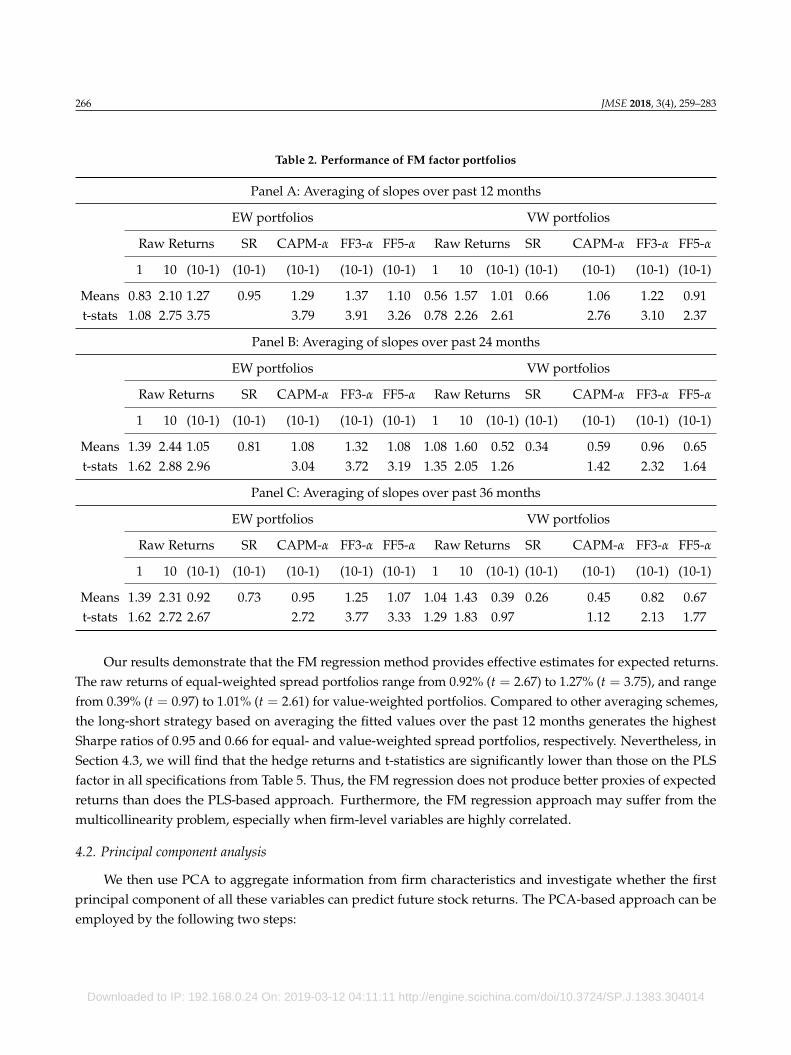
Table 2 shows time series averages (raw returns, Sharpe ratios, CAPM α, FF3 α, FF5 α) and t-statisticsof monthly equal-weighted (EW) and value-weighted (VW) stock returns on decile portfolios formed by FMestimates expected returns. The columns (10-1) report the statistics for the difference in returns on the topand bottom portfolios. The expected returns are estimated using fitted value of regressions, and the panelscorrespond to different time series averaging schemes for the slopes of the Fama-MacBeth regression. Thesample is from July 2001 to December 2016 for Panel A. For Panel B and C, the sample is from July 2003 toDecember 2016. The portfolios are rebalanced monthly. All returns and alphas are reported in percentagepoints.


266 JMSE 2018, 3(4), 259–283

Table 2. Performance of FM factor portfolios

Panel A: Averaging of slopes over past 12 months

EW portfolios VW portfolios

Raw Returns SR CAPM-α FF3-α FF5-α Raw Returns SR CAPM-α FF3-α FF5-α

1 10 (10-1) (10-1) (10-1) (10-1) (10-1) 1 10 (10-1) (10-1) (10-1) (10-1) (10-1)

Means 0.83 2.10 1.27 0.95 1.29 1.37 1.10 0.56 1.57 1.01 0.66 1.06 1.22 0.91t-stats 1.08 2.75 3.75 3.79 3.91 3.26 0.78 2.26 2.61 2.76 3.10 2.37

Panel B: Averaging of slopes over past 24 months



1 10 (10-1) (10-1) (10-1) (10-1) (10-1) 1 10 (10-1) (10-1) (10-1) (10-1) (10-1)

Means 1.39 2.44 1.05 0.81 1.08 1.32 1.08 1.08 1.60 0.52 0.34 0.59 0.96 0.65t-stats 1.62 2.88 2.96 3.04 3.72 3.19 1.35 2.05 1.26 1.42 2.32 1.64

Panel C: Averaging of slopes over past 36 months



1 10 (10-1) (10-1) (10-1) (10-1) (10-1) 1 10 (10-1) (10-1) (10-1) (10-1) (10-1)

Means 1.39 2.31 0.92 0.73 0.95 1.25 1.07 1.04 1.43 0.39 0.26 0.45 0.82 0.67t-stats 1.62 2.72 2.67 2.72 3.77 3.33 1.29 1.83 0.97 1.12 2.13 1.77

Our results demonstrate that the FM regression method provides effective estimates for expected returns.The raw returns of equal-weighted spread portfolios range from 0.92% (t = 2.67) to 1.27% (t = 3.75), and rangefrom 0.39% (t = 0.97) to 1.01% (t = 2.61) for value-weighted portfolios. Compared to other averaging schemes,the long-short strategy based on averaging the fitted values over the past 12 months generates the highestSharpe ratios of 0.95 and 0.66 for equal- and value-weighted spread portfolios, respectively. Nevertheless, inSection 4.3, we will find that the hedge returns and t-statistics are significantly lower than those on the PLSfactor in all specifications from Table 5. Thus, the FM regression does not produce better proxies of expectedreturns than does the PLS-based approach. Furthermore, the FM regression approach may suffer from themulticollinearity problem, especially when firm-level variables are highly correlated.

4.2. Principal component analysis

We then use PCA to aggregate information from firm characteristics and investigate whether the firstprincipal component of all these variables can predict future stock returns. The PCA-based approach can beemployed by the following two steps:


JMSE 2018, 3(4), 259–283 267

Step 1. Apply PCA to the standardized firm characteristics Xait and compute the coefficients of the first

principal component βa(pca), a = 1, . . ., A with a representing each firm characteristic, and A is the total number

of firm characteristics. In this study, we set A equal to 75.Step 2. Calculate a potential predictor of returns as

r̂(pca)it =A

∑a=1

(∑s∈T

βa(pca)s

)Xa

it, (1)

where the coefficients βa(pca)s are averaged over the past 12 months, the past 24 months, and the past 36 months.

Then, at the beginning of each month, we sort stocks into 10 decile portfolios on the predictor r̂(pca)it andrebalance in the next month.

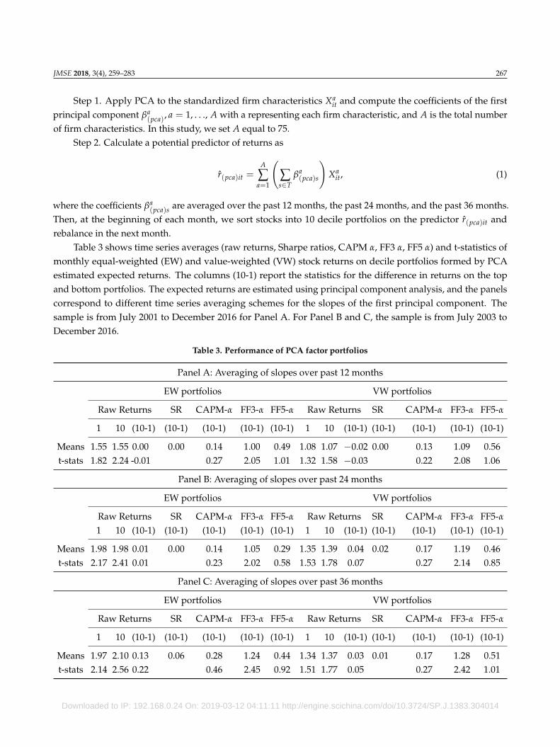
Table 3 shows time series averages (raw returns, Sharpe ratios, CAPM α, FF3 α, FF5 α) and t-statistics ofmonthly equal-weighted (EW) and value-weighted (VW) stock returns on decile portfolios formed by PCAestimated expected returns. The columns (10-1) report the statistics for the difference in returns on the topand bottom portfolios. The expected returns are estimated using principal component analysis, and the panelscorrespond to different time series averaging schemes for the slopes of the first principal component. Thesample is from July 2001 to December 2016 for Panel A. For Panel B and C, the sample is from July 2003 toDecember 2016.

Table 3. Performance of PCA factor portfolios




1 10 (10-1) (10-1) (10-1) (10-1) (10-1) 1 10 (10-1) (10-1) (10-1) (10-1) (10-1)

Means 1.55 1.55 0.00 0.00 0.14 1.00 0.49 1.08 1.07 −0.02 0.00 0.13 1.09 0.56t-stats 1.82 2.24 -0.01 0.27 2.05 1.01 1.32 1.58 −0.03 0.22 2.08 1.06



Raw Returns SR CAPM-α FF3-α FF5-α Raw Returns SR CAPM-α FF3-α FF5-α1 10 (10-1) (10-1) (10-1) (10-1) (10-1) 1 10 (10-1) (10-1) (10-1) (10-1) (10-1)

Means 1.98 1.98 0.01 0.00 0.14 1.05 0.29 1.35 1.39 0.04 0.02 0.17 1.19 0.46t-stats 2.17 2.41 0.01 0.23 2.02 0.58 1.53 1.78 0.07 0.27 2.14 0.85




1 10 (10-1) (10-1) (10-1) (10-1) (10-1) 1 10 (10-1) (10-1) (10-1) (10-1) (10-1)

Means 1.97 2.10 0.13 0.06 0.28 1.24 0.44 1.34 1.37 0.03 0.01 0.17 1.28 0.51t-stats 2.14 2.56 0.22 0.46 2.45 0.92 1.51 1.77 0.05 0.27 2.42 1.01


268 JMSE 2018, 3(4), 259–283

Table 3 implies that the first principal component of PCA is a poor predictor of future stock returns.Both equal- and value-weighted spread portfolios cannot produce significant raw returns when the averagingwindows are 12 months, 24 months, and 36 months. Moreover, the Sharpe ratios of the above long-shortstrategies tend to be 0. The FF5 alphas vary from 0.29% (t = 0.58) to 0.49% (t = 1.01) for equal-weighted spreadportfolios, and vary from 0.46% (t = 0.85) to 0.56% (t = 1.06) for value-weighted spread portfolios, whichmeans none of them are statistically significant. Therefore, the PCA approach indeed underperforms the FMregression approach. These results indicate that the firm-level variables that share returns-unrelated commonvariation will contaminate the first principal component and decrease its return predictability.

4.3. Forecast combination

In this subsection, we employ the FC approach to summarize the expected returns. The core idea of thisapproach is to compute equal-weighted fitted values from individual regressions of realized returns on eachlagged firm characteristic.

In the first step, we run 75 separate regressions of returns on each characteristic lagged in each month.Then, we use the slope of each firm characteristic to calculate the fitted value from each regression, which isthe standardized firm characteristic multiplied by its estimated coefficient from the regressions. Therefore, theexpected return of each stock is the equal-weighted mean of these fitted values of 75 firm characteristics. Similarto FM regression, we consider three types of fitted values: the regression slopes are averaged over the past 12months, the past 24 months, and the past 36 months. We then sort stocks into 10 decile portfolios on the forecastcombination of fitted values and rebalance the portfolios monthly.

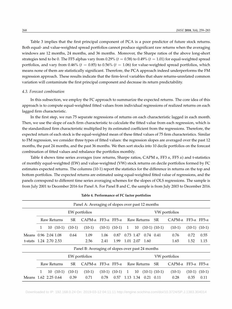
Table 4 shows time series averages (raw returns, Sharpe ratios, CAPM α, FF3 α, FF5 α) and t-statisticsof monthly equal-weighted (EW) and value-weighted (VW) stock returns on decile portfolios formed by FCestimates expected returns. The columns (10-1) report the statistics for the difference in returns on the top andbottom portfolios. The expected returns are estimated using equal-weighted fitted value of regressions, and thepanels correspond to different time series averaging schemes for the slopes of OLS regressions. The sample isfrom July 2001 to December 2016 for Panel A. For Panel B and C, the sample is from July 2003 to December 2016.

Table 4. Performance of FC factor portfolios




1 10 (10-1) (10-1) (10-1) (10-1) (10-1) 1 10 (10-1) (10-1) (10-1) (10-1) (10-1)

Means 0.96 2.04 1.08 0.64 1.09 1.06 0.87 0.73 1.47 0.74 0.41 0.76 0.72 0.55t-stats 1.24 2.70 2.53 2.56 2.41 1.99 1.01 2.07 1.60 1.65 1.52 1.15




1 10 (10-1) (10-1) (10-1) (10-1) (10-1) 1 10 (10-1) (10-1) (10-1) (10-1) (10-1)Means 1.62 2.25 0.64 0.39 0.71 0.78 0.57 1.13 1.34 0.21 0.11 0.28 0.35 0.11


JMSE 2018, 3(4), 259–283 269

Table 4. Cont.

t-stats 1.85 2.67 1.42 1.59 1.69 1.24 1.41 1.71 0.41 0.55 0.67 0.21




1 10 (10-1) (10-1) (10-1) (10-1) (10-1) 1 10 (10-1) (10-1) (10-1) (10-1) (10-1)

Means 1.55 2.07 0.52 0.34 0.63 1.06 0.75 1.15 1.31 0.15 0.08 0.26 0.72 0.35t-stats 1.74 2.53 1.24 1.52 2.71 1.96 1.39 1.71 0.30 0.53 1.53 0.76

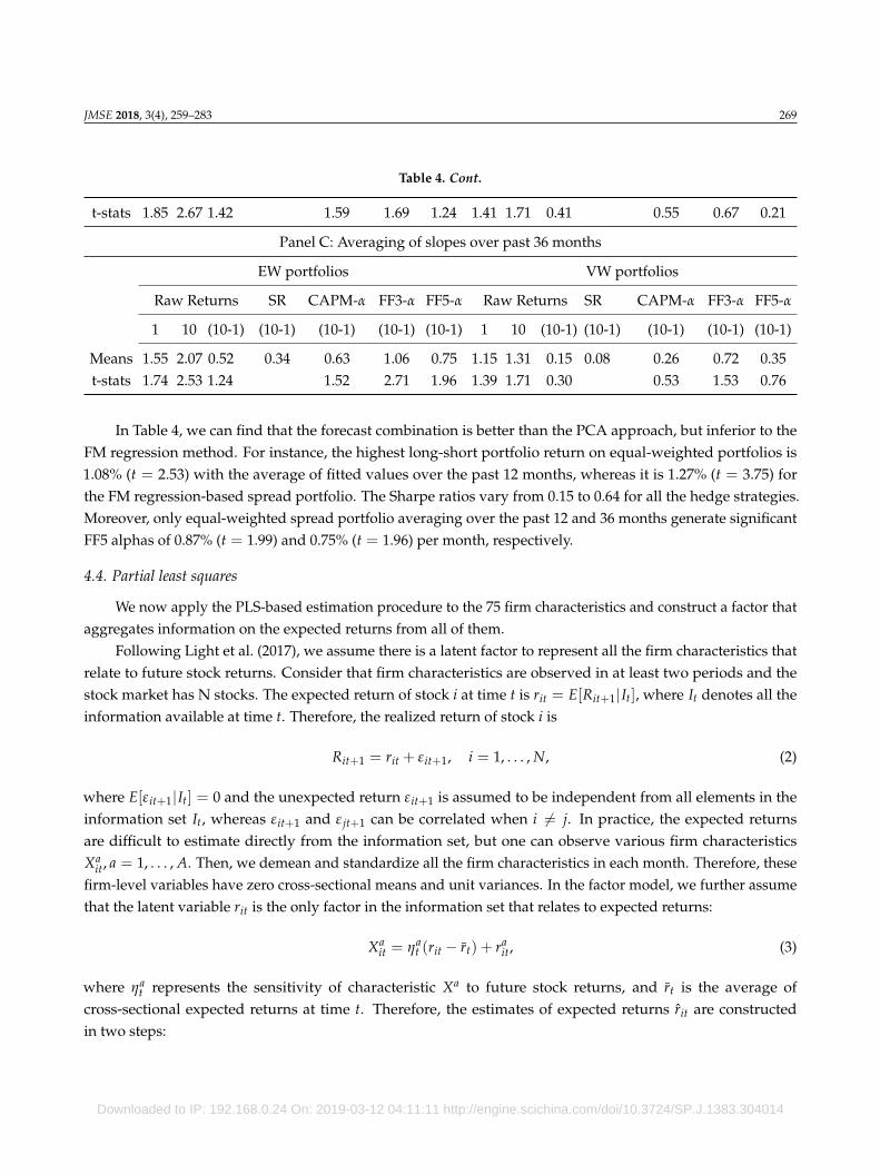
In Table 4, we can find that the forecast combination is better than the PCA approach, but inferior to theFM regression method. For instance, the highest long-short portfolio return on equal-weighted portfolios is1.08% (t = 2.53) with the average of fitted values over the past 12 months, whereas it is 1.27% (t = 3.75) forthe FM regression-based spread portfolio. The Sharpe ratios vary from 0.15 to 0.64 for all the hedge strategies.Moreover, only equal-weighted spread portfolio averaging over the past 12 and 36 months generate significantFF5 alphas of 0.87% (t = 1.99) and 0.75% (t = 1.96) per month, respectively.

4.4. Partial least squares

We now apply the PLS-based estimation procedure to the 75 firm characteristics and construct a factor thataggregates information on the expected returns from all of them.

Following Light et al. (2017), we assume there is a latent factor to represent all the firm characteristics thatrelate to future stock returns. Consider that firm characteristics are observed in at least two periods and thestock market has N stocks. The expected return of stock i at time t is rit = E[Rit+1|It], where It denotes all theinformation available at time t. Therefore, the realized return of stock i is

Rit+1 = rit + εit+1, i = 1, . . . , N, (2)

where E[εit+1|It] = 0 and the unexpected return εit+1 is assumed to be independent from all elements in theinformation set It, whereas εit+1 and ε jt+1 can be correlated when i 6= j. In practice, the expected returnsare difficult to estimate directly from the information set, but one can observe various firm characteristicsXa

it, a = 1, . . . , A. Then, we demean and standardize all the firm characteristics in each month. Therefore, thesefirm-level variables have zero cross-sectional means and unit variances. In the factor model, we further assumethat the latent variable rit is the only factor in the information set that relates to expected returns:

Xait = ηa

t (rit − r̄t) + rait, (3)

where ηat represents the sensitivity of characteristic Xa to future stock returns, and r̄t is the average of

cross-sectional expected returns at time t. Therefore, the estimates of expected returns r̂it are constructedin two steps:


270 JMSE 2018, 3(4), 259–283

Step 1. Run separate cross-sectional regressions of R̂it, i = 1, . . . , N on each individual firm-level variableXa

it−1, a = 1, . . . , N for a = 1, . . . , A and denote the obtained slopes as βat .

Step 2. For each firm i, i = 1, . . . , N, run a regression of Xait on βa

t , a = 1, . . . , A, and denote the obtainedslopes as r̂it.

The expected returns can be less biased and estimated more precisely if we use information of characteristicsand not only from data in periods t and t− 1. Therefore, we calculate particular time series averages of βs

t , s ≤ tin the first step and use them in the regression of the second step instead of βa

t . Specifically, we separatelyconsider the different versions of the PLS-based factor on the averages of βa

s over the past 12 months, past 24months, and past 36 months.

To explore the relation between the PLS factor and expected stock returns, we employ the same approachas we use in the univariate portfolio analysis for individual firm characteristics. At the beginning of each month,we sort firms into 10 decile portfolios according to the PLS factor estimation of expected returns, hold for onemonth and calculate the monthly portfolio returns. Particularly, decile 1 refers to firms in the lowest decile anddecile 10 to firms in the highest decile. The “(10− 1)” spread portfolio is computed as long the highest decileand short the lowest decile.

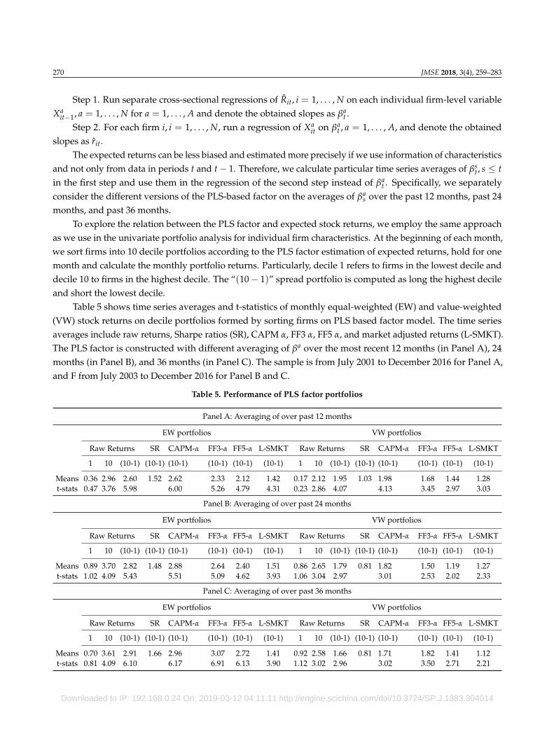
Table 5 shows time series averages and t-statistics of monthly equal-weighted (EW) and value-weighted(VW) stock returns on decile portfolios formed by sorting firms on PLS based factor model. The time seriesaverages include raw returns, Sharpe ratios (SR), CAPM α, FF3 α, FF5 α, and market adjusted returns (L-SMKT).The PLS factor is constructed with different averaging of βa over the most recent 12 months (in Panel A), 24months (in Panel B), and 36 months (in Panel C). The sample is from July 2001 to December 2016 for Panel A,and F from July 2003 to December 2016 for Panel B and C.

Table 5. Performance of PLS factor portfolios

Panel A: Averaging of over past 12 months


Raw Returns SR CAPM-α FF3-α FF5-α L-SMKT Raw Returns SR CAPM-α FF3-α FF5-α L-SMKT

1 10 (10-1) (10-1) (10-1) (10-1) (10-1) (10-1) 1 10 (10-1) (10-1) (10-1) (10-1) (10-1) (10-1)

Means 0.36 2.96 2.60 1.52 2.62 2.33 2.12 1.42 0.17 2.12 1.95 1.03 1.98 1.68 1.44 1.28t-stats 0.47 3.76 5.98 6.00 5.26 4.79 4.31 0.23 2.86 4.07 4.13 3.45 2.97 3.03

Panel B: Averaging of over past 24 months



1 10 (10-1) (10-1) (10-1) (10-1) (10-1) (10-1) 1 10 (10-1) (10-1) (10-1) (10-1) (10-1) (10-1)

Means 0.89 3.70 2.82 1.48 2.88 2.64 2.40 1.51 0.86 2.65 1.79 0.81 1.82 1.50 1.19 1.27t-stats 1.02 4.09 5.43 5.51 5.09 4.62 3.93 1.06 3.04 2.97 3.01 2.53 2.02 2.33

Panel C: Averaging of over past 36 months



1 10 (10-1) (10-1) (10-1) (10-1) (10-1) (10-1) 1 10 (10-1) (10-1) (10-1) (10-1) (10-1) (10-1)

Means 0.70 3.61 2.91 1.66 2.96 3.07 2.72 1.41 0.92 2.58 1.66 0.81 1.71 1.82 1.41 1.12t-stats 0.81 4.09 6.10 6.17 6.91 6.13 3.90 1.12 3.02 2.96 3.02 3.50 2.71 2.21


JMSE 2018, 3(4), 259–283 271

In Panel A of Table 5, we find that the PLS factor-based equal-weighted portfolios’ monthly averageraw returns increase from 0.36% to 2.96% from the lowest to the highest decile. The average return of theequal-weighted spread portfolio is 2.60% (t = 5.98) per month, which indicates that the long-short tradingstrategy of buying the highest and selling the lowest deciles will earn annual returns of about 31.20% onaverage. Moreover, the Sharpe ratio of this strategy achieves 1.52, which means comparatively large andsteady investment benefits. Our results also show strong and positive PLS-based premium. Specifically, theequal-weighted spread portfolio has a monthly CAPM alpha of 2.62% (t = 6.00), a monthly FF3 alpha of 2.33%(t = 5.26), and a monthly FF5 alpha of 2.12% (t = 4.79). Some practitioners argue that it is hard to short a stockin the Chinese market because of the short sell restrictions. Hence, we propose a new strategy of buying thehighest PLS factor-based portfolio and short the value-weighted aggregate market portfolio, and compute thespread portfolio return denoted as market adjusted return (L-SMKT). The monthly market adjusted return ofthe equal-weighted portfolio is 1.42% (t = 4.31), which is lower than the normal long-short portfolio but stillstatistically significant. The right-hand side of Panel A represents the results on PLS-based value-weightedportfolios. The spread portfolio generates a monthly raw return of 1.95% (t = 4.07), a monthly market adjustedreturn of 1.28% (t = 3.03), with a Sharpe ratio of 1.03. The CAPM, FF3, and FF5 alphas of spread portfolio are1.98% (t = 4.13), 1.68% (t = 3.45), and 1.44% (t = 2.97).

Panels B and C of Table 5 report similar findings when we obtain the PLS factor by using averages ofβa

s over the past 24 months and past 36 months. For example, the equal-weighted spread portfolio monthlyreturns range from 2.82% (t = 5.43) to 2.91% (t = 6.10), and the FF5 alphas range from 2.40% (t = 4.62) to 2.72%(t = 6.13) per month. For value-weighted spread portfolios, the raw returns, adjusted market returns, andthe abnormal returns are lower than those in Panel A, but still economically large and statistically significant.Thus, our results imply that all the 75 firm characteristics in the Chinese stock market indeed share the expectedreturn-related latent factor, which can be viewed as a commonality in the cross-sectional anomalies associatedwith various firm-level signals. In addition, the PLS factor method outperforms the FM regression, PCA, andforecast combination approaches in forecasting the China market.

4.5. Economic explanations for the PLS performance

Section 4.4 shows that the PLS method outperforms the PCA, FM, and FC approaches in forecasting thecross-sectional Chinese stock returns. In this section, we seek to provide more economic motivations for PLS’superior performance.

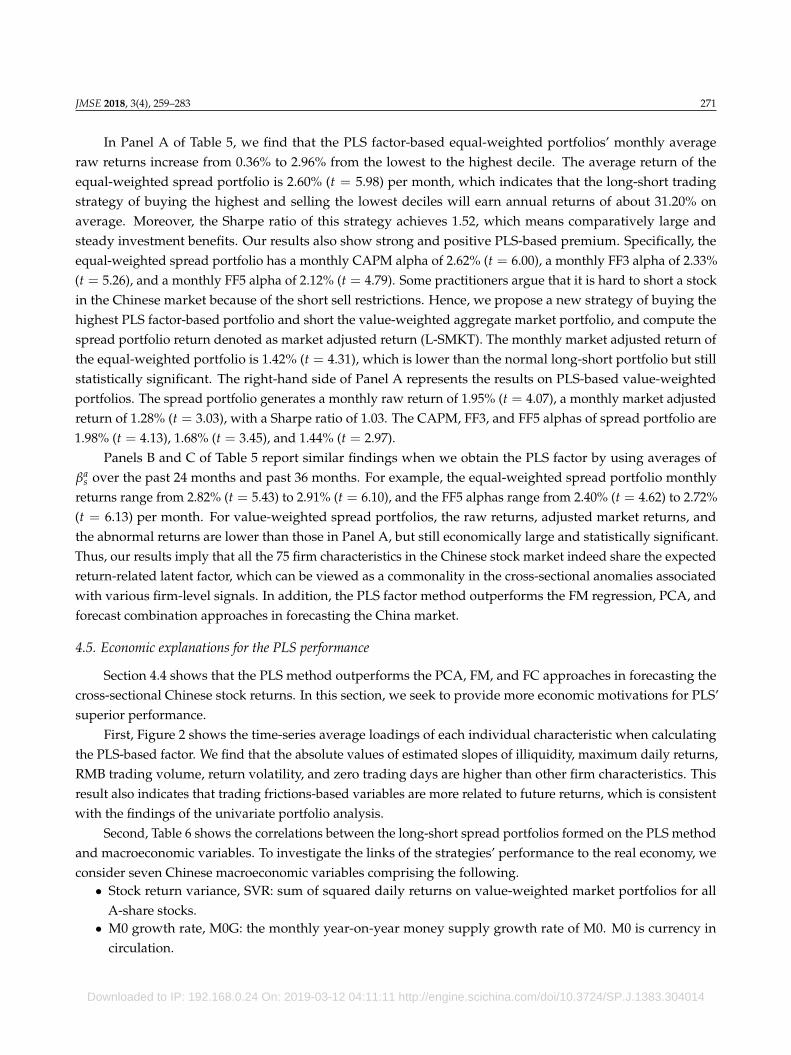
First, Figure 2 shows the time-series average loadings of each individual characteristic when calculatingthe PLS-based factor. We find that the absolute values of estimated slopes of illiquidity, maximum daily returns,RMB trading volume, return volatility, and zero trading days are higher than other firm characteristics. Thisresult also indicates that trading frictions-based variables are more related to future returns, which is consistentwith the findings of the univariate portfolio analysis.

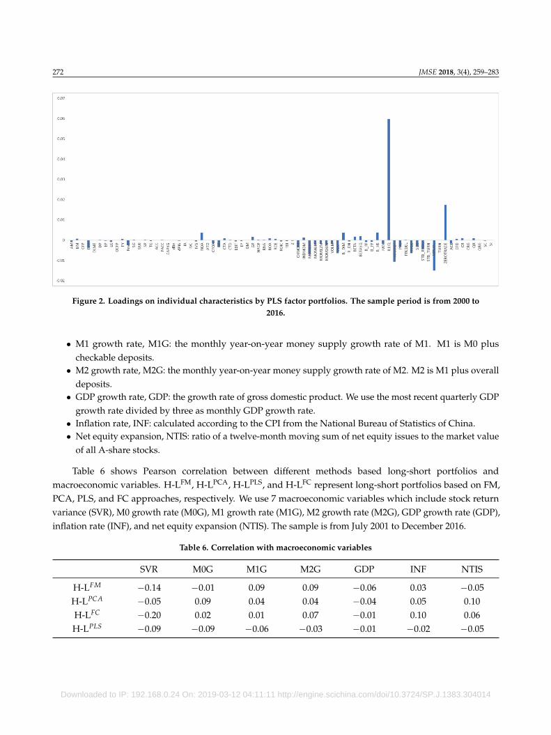
Second, Table 6 shows the correlations between the long-short spread portfolios formed on the PLS methodand macroeconomic variables. To investigate the links of the strategies’ performance to the real economy, weconsider seven Chinese macroeconomic variables comprising the following.• Stock return variance, SVR: sum of squared daily returns on value-weighted market portfolios for all

A-share stocks.• M0 growth rate, M0G: the monthly year-on-year money supply growth rate of M0. M0 is currency in

circulation.


272 JMSE 2018, 3(4), 259–283

Figure 2. Loadings on individual characteristics by PLS factor portfolios. The sample period is from 2000 to2016.

• M1 growth rate, M1G: the monthly year-on-year money supply growth rate of M1. M1 is M0 pluscheckable deposits.

• M2 growth rate, M2G: the monthly year-on-year money supply growth rate of M2. M2 is M1 plus overalldeposits.

• GDP growth rate, GDP: the growth rate of gross domestic product. We use the most recent quarterly GDPgrowth rate divided by three as monthly GDP growth rate.

• Inflation rate, INF: calculated according to the CPI from the National Bureau of Statistics of China.• Net equity expansion, NTIS: ratio of a twelve-month moving sum of net equity issues to the market value

of all A-share stocks.

Table 6 shows Pearson correlation between different methods based long-short portfolios andmacroeconomic variables. H-LFM, H-LPCA, H-LPLS, and H-LFC represent long-short portfolios based on FM,PCA, PLS, and FC approaches, respectively. We use 7 macroeconomic variables which include stock returnvariance (SVR), M0 growth rate (M0G), M1 growth rate (M1G), M2 growth rate (M2G), GDP growth rate (GDP),inflation rate (INF), and net equity expansion (NTIS). The sample is from July 2001 to December 2016.

Table 6. Correlation with macroeconomic variables

SVR M0G M1G M2G GDP INF NTIS

H-LFM −0.14 −0.01 0.09 0.09 −0.06 0.03 −0.05H-LPCA −0.05 0.09 0.04 0.04 −0.04 0.05 0.10H-LFC −0.20 0.02 0.01 0.07 −0.01 0.10 0.06H-LPLS −0.09 −0.09 −0.06 −0.03 −0.01 −0.02 −0.05


JMSE 2018, 3(4), 259–283 273

Table 6 shows that the PLS factor has negative correlations with the seven economic variables, includingstock return variance (SVR), M0 growth rate (M0G), M1 growth rate (M1G), M2 growth rate (M2G), GDP growthrate (GDP), inflation rate (INF), and net equity expansion (NTIS), with the correlation coefficient up to -0.09.The results indicate that the PLS factor generally is countercyclical, while the results for the FM, PCA, and FCfactors are mixed.

Third, econometrically, Light et al. (2017) show that the main objective of PLS is to extract from a large setof predictors a common factor that has the highest covariance with the predicted variable. This is a “disciplined”dimension reduction technique. PLS identifies a factor with the best ability to predict the target variableeven though this factor may not be the best in describing the correlations between predictors. While thePCA approach extracts one factor that explains the most important source of common variation in predictivevariables, it may include common noise, which is unrelated to predicting the target variable. Therefore, PLSoutperforms the PCA approach in predicting future returns.

The PLS approach likely is more efficient that the FM approach because it assumes a parsimonious factorstructure, while FM regression estimates may have overfitting problems when the number of firm characteristicsis large. Moreover, because some firm characteristics are highly correlated with each other, the FM approach willhave a serious multicollinearity problem. The FC approach averages the univariate predictive regression valuesof firm characteristics equally, but it ignores the multivariate information structure and interaction between firmcharacteristics. Hence, it may have an underfitting problem and will lead to a less accurate prediction as well.

In all, the PLS approach in this study is similar to the three-pass regression filter (3PRF) developed by Kellyand Pruitt (2015). We estimate expected returns on all stocks based on current characteristics, but use laggedcharacteristics to estimate the loadings. The loadings are allowed to vary over time. This approach is moreeffective in aggregating information for a cross-sectional analysis, and so it makes more accurate future returnpredictions.

4.6. Performance of different factor categories

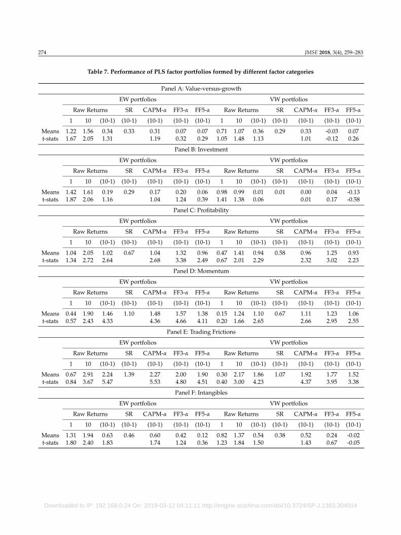
In this subsection, we investigate the performance of anomalies based on their different categories. Asmentioned in Section 2, we classify all the individual firm characteristics into six categories comprisingvalue-versus-growth, investment, profitability, momentum, trading frictions, and intangibles. Table 7 shows thetime series averages (raw returns, Sharpe ratios, CAPM α, FF3 α, and FF5 α) and t-statistics of monthly equal-and value-weighted stock returns on decile portfolios formed by sorting firms on the PLS-based factor modelwith the average of βa over the past 12 months.

Our results indicate that anomalies belonging to trading frictions, momentum, and profitability are moreeffective to aggregate the cross-sectional expected returns in the Chinese stock market. Specifically, tradingfrictions-based spread portfolios generate 2.24% (t = 5.47) and 1.86% (t = 4.23) equal- and value-weightedraw returns per month, respectively. Momentum-based spread portfolios produce 1.46% (t = 4.33) and 1.10%(t = 2.65) equal- and value-weighted monthly returns, respectively, while the profitability-based long-shortportfolio equal- and value-weighted returns are 1.02% (t = 2.64%) and 0.94 (t = 2.29), respectively. The Sharperatios of trading frictions-based long-short strategies range from 1.07 to 1.39, which represent the highest Sharperatios among all the categories. On the contrary, neither equal-weighted nor value-weighted spread portfoliosbased on value-versus-growth, investment, and intangibles can generate significant raw returns.


274 JMSE 2018, 3(4), 259–283

Table 7. Performance of PLS factor portfolios formed by different factor categories

Panel A: Value-versus-growth



1 10 (10-1) (10-1) (10-1) (10-1) (10-1) 1 10 (10-1) (10-1) (10-1) (10-1) (10-1)

Means 1.22 1.56 0.34 0.33 0.31 0.07 0.07 0.71 1.07 0.36 0.29 0.33 -0.03 0.07t-stats 1.67 2.05 1.31 1.19 0.32 0.29 1.05 1.48 1.13 1.01 -0.12 0.26

Panel B: Investment



1 10 (10-1) (10-1) (10-1) (10-1) (10-1) 1 10 (10-1) (10-1) (10-1) (10-1) (10-1)

Means 1.42 1.61 0.19 0.29 0.17 0.20 0.06 0.98 0.99 0.01 0.01 0.00 0.04 -0.13t-stats 1.87 2.06 1.16 1.04 1.24 0.39 1.41 1.38 0.06 0.01 0.17 -0.58

Panel C: Profitability



1 10 (10-1) (10-1) (10-1) (10-1) (10-1) 1 10 (10-1) (10-1) (10-1) (10-1) (10-1)

Means 1.04 2.05 1.02 0.67 1.04 1.32 0.96 0.47 1.41 0.94 0.58 0.96 1.25 0.93t-stats 1.34 2.72 2.64 2.68 3.38 2.49 0.67 2.01 2.29 2.32 3.02 2.23

Panel D: Momentum



1 10 (10-1) (10-1) (10-1) (10-1) (10-1) 1 10 (10-1) (10-1) (10-1) (10-1) (10-1)

Means 0.44 1.90 1.46 1.10 1.48 1.57 1.38 0.15 1.24 1.10 0.67 1.11 1.23 1.06t-stats 0.57 2.43 4.33 4.36 4.66 4.11 0.20 1.66 2.65 2.66 2.95 2.55

Panel E: Trading Frictions



1 10 (10-1) (10-1) (10-1) (10-1) (10-1) 1 10 (10-1) (10-1) (10-1) (10-1) (10-1)

Means 0.67 2.91 2.24 1.39 2.27 2.00 1.90 0.30 2.17 1.86 1.07 1.92 1.77 1.52t-stats 0.84 3.67 5.47 5.53 4.80 4.51 0.40 3.00 4.23 4.37 3.95 3.38

Panel F: Intangibles



1 10 (10-1) (10-1) (10-1) (10-1) (10-1) 1 10 (10-1) (10-1) (10-1) (10-1) (10-1)

Means 1.31 1.94 0.63 0.46 0.60 0.42 0.12 0.82 1.37 0.54 0.38 0.52 0.24 -0.02t-stats 1.80 2.40 1.83 1.74 1.24 0.36 1.23 1.84 1.50 1.43 0.67 -0.05


JMSE 2018, 3(4), 259–283 275

5. Conclusion

In this study, we create for the first time a large set of 75 firm characteristics in the Chinese stock market.We then apply the latest “big-data” methods to extract and aggregate forecasting information from the 75firm characteristics for predicting the cross section of expected Chinese stock returns. Empirically, we findthat firm characteristics have statistically and economically forecasting power. In comparing the “big-data”methods, we find that PLS is the most efficient one in aggregating the information from all the characteristics.The long-short portfolio returns produced by using PLS are economically large and statistically significant, andperform better than all the firm characteristics individually, even if one chooses them ex post. We also find thatfirm characteristics related to trading frictions, momentum, and profitability have stronger forecasting powerfor expected Chinese stock returns. While there are ample studies in the US to understand the role of firmcharacteristics in asset pricing, our paper provides the first empirical evidence on the value of a comprehensiveset of characteristics in the Chinese stock market, and also highlights the usefulness of novel machine-learningtechniques to aggregate big-data information in the stock market. Future studies could focus on the incrementalpredictive information of each characteristic variable to better understand the economic link and structure ofthe vast anomalies in the Chinese stock market.

Acknowledgments: We are grateful to seminar participants at Beijing University, Central University of Finance andEconomics, Georgia State University, Hunan University, Indiana University, Renmin University, Shanghai University ofFinance and Economics, Washington University in St. Louis, and conference participants at the 2018 Conference on FinancialPredictability and Big Data for insightful comments. We are also grateful to the editors of the special issue, and especially totwo anonymous referees for their very thoughtful and helpful comments that have helped improve the paper substantially.We acknowledge the financial support from National Natural Science Foundation of China (No. 71872195, 71602198), BeijingNatural Science Foundation (No. 9174045), Hunan Natural Science Foundation (No. 2019JJ50058) and the FundamentalResearch Funds for the Central Universities.Conflicts of Interest: The authors declare no conflict of interest.

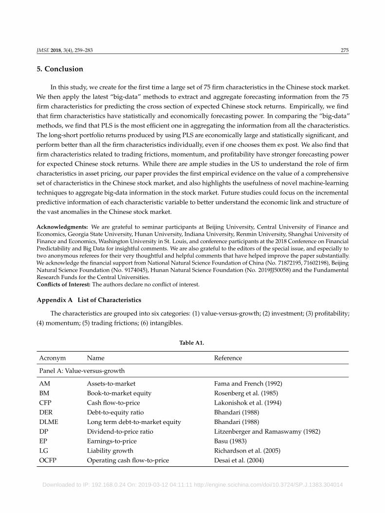
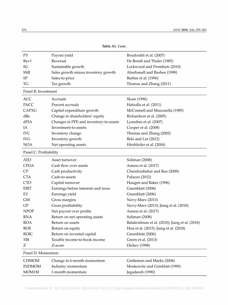
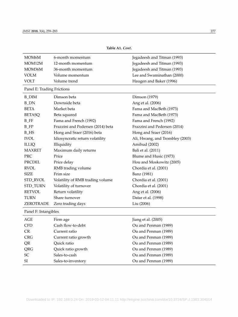
Appendix A List of Characteristics

The characteristics are grouped into six categories: (1) value-versus-growth; (2) investment; (3) profitability;(4) momentum; (5) trading frictions; (6) intangibles.

Table A1.

Acronym Name Reference

Panel A: Value-versus-growth

AM Assets-to-market Fama and French (1992)BM Book-to-market equity Rosenberg et al. (1985)CFP Cash flow-to-price Lakonishok et al. (1994)DER Debt-to-equity ratio Bhandari (1988)DLME Long term debt-to-market equity Bhandari (1988)DP Dividend-to-price ratio Litzenberger and Ramaswamy (1982)EP Earnings-to-price Basu (1983)LG Liability growth Richardson et al. (2005)OCFP Operating cash flow-to-price Desai et al. (2004)


276 JMSE 2018, 3(4), 259–283

Table A1. Cont.

PY Payout yield Boudoukh et al. (2007)Rev1 Reversal De Bondt and Thaler (1985)SG Sustainable growth Lockwood and Prombutr (2010)SMI Sales growth minus inventory growth Abarbanell and Bushee (1998)SP Sales-to-price Barbee et al. (1996)TG Tax growth Thomas and Zhang (2011)

Panel B: Investment

ACC Accruals Sloan (1996)PACC Percent accruals Hafzalla et al. (2011)CAPXG Capital expenditure growth McConnell and Muscarella (1985)dBe Change in shareholders’ equity Richardson et al. (2005)dPIA Changes in PPE and inventory-to-assets Lyandres et al. (2007)IA Investment-to-assets Cooper et al. (2008)IVC Inventory change Thomas and Zhang (2002)IVG Inventory growth Belo and Lin (2012)NOA Net operating assets Hirshleifer et al. (2004)

Panel C: Profitability

ATO Asset turnover Soliman (2008)CFOA Cash flow over assets Asness et al. (2017)CP Cash productivity Chandrashekar and Rao (2009)CTA Cash-to-assets Palazzo (2012)CTO Capital turnover Haugen and Baker (1996)EBIT Earnings before interests and taxes Greenblatt (2006)EY Earnings yield Greenblatt (2006)GM Gross margins Novy-Marx (2013)GP Gross profitability Novy-Marx (2013); Jiang et al. (2018)NPOP Net payout over profits Asness et al. (2017)RNA Return on net operating assets Soliman (2008)ROA Return on assets Balakrishnan et al. (2010); Jiang et al. (2018)ROE Return on equity Hou et al. (2015); Jiang et al. (2018)ROIC Return on invested capital Greenblatt (2006)TBI Taxable income-to-book income Green et al. (2013)Z Z-score Dichev (1998)

Panel D: Momentum

CHMOM Change in 6-month momentum Gettleman and Marks (2006)INDMOM Industry momentum Moskowitz and Grinblatt (1999)MOM1M 1-month momentum Jegadeesh (1990)


JMSE 2018, 3(4), 259–283 277

Table A1. Cont.

MOM6M 6-month momentum Jegadeesh and Titman (1993)MOM12M 12-month momentum Jegadeesh and Titman (1993)MOM36M 36-month momentum Jegadeesh and Titman (1993)VOLM Volume momentum Lee and Swaminathan (2000)VOLT Volume trend Haugen and Baker (1996)

Panel E: Trading Frictions

B_DIM Dimson beta Dimson (1979)B_DN Downside beta Ang et al. (2006)BETA Market beta Fama and MacBeth (1973)BETASQ Beta squared Fama and MacBeth (1973)B_FF Fama and French (1992) Fama and French (1992)B_FP Frazzini and Pedersen (2014) beta Frazzini and Pedersen (2014)B_HS Hong and Sraer (2016) beta Hong and Sraer (2016)IVOL Idiosyncratic return volatility Ali, Hwang, and Trombley (2003)ILLIQ Illiquidity Amihud (2002)MAXRET Maximum daily returns Bali et al. (2011)PRC Price Blume and Husic (1973)PRCDEL Price delay Hou and Moskowitz (2005)RVOL RMB trading volume Chordia et al. (2001)SIZE Frim size Banz (1981)STD_RVOL Volatility of RMB trading volume Chordia et al. (2001)STD_TURN Volatility of turnover Chordia et al. (2001)RETVOL Return volatility Ang et al. (2006)TURN Share turnover Datar et al. (1998)ZEROTRADE Zero trading days Liu (2006)

Panel F: Intangibles

AGE Firm age Jiang et al. (2005)CFD Cash flow-to-debt Ou and Penman (1989)CR Current ratio Ou and Penman (1989)CRG Current ratio growth Ou and Penman (1989)QR Quick ratio Ou and Penman (1989)QRG Quick ratio growth Ou and Penman (1989)SC Sales-to-cash Ou and Penman (1989)SI Sales-to-inventory Ou and Penman (1989)


278 JMSE 2018, 3(4), 259–283

Appendix B Definitions of Characteristics

This section provides the detailed definitions of the variables employed in this study. All the accountingvariables are constructed from the CSMAR database. The annual statements are assumed to be publicly availableby the end of June in the calendar year t+1 for the fiscal year t, while data from quarterly statements are updatedmonthly using the most recently announced quarterly accounting information.

AM: Assets-to-market, which is total assets for the fiscal year divided by fiscal year-end market capitalization.BM: Book-to-market equity, which is the book value of equity for fiscal year divided by fiscal year-end market

capitalization.CFP: Cash flow-to-price, which is operating cash flows divided by fiscal year-end market capitalization.DER: Debt-to-equity ratio, which is total liabilities divided by fiscal year-end market capitalization.DLME: Long term debt-to-market equity, which is long term liabilities divided by fiscal year-end market

capitalization.DP: Dividend-to-price ratio, which is annual total dividends payouts divided by fiscal year-end market

capitalization.EP: Earnings-to-price, which is annual income before extraordinary items divided by fiscal year-end market

capitalization.LG: Liability growth, which is the annual change in total liabilities divided by 1 year-lagged total liabilities.OCFP: Operating cash flow-to-price, which is operating cash flow divided by fiscal year-end market

capitalization.PY: Payout yield, which is annual income before extraordinary items minus the change of book equity divided

by fiscal year-end market capitalization.Rev1: Reversal, which is cumulative returns from months t-60 to t-13.SG: Sustainable growth, which is annual growth in book value of equity.SMI: Sales growth minus inventory growth, which is annual growth in sales minus annual growth in inventory.SP: Sales-to-price, which is the annual operating revenue divided by fiscal year-end market capitalization.TG: Tax growth, which is annual change in taxes payable divided by 1 year-lagged taxes payable.ACC: Accruals, which is annual income before extraordinary items minus operating cash flows divided by

average total assets.PACC: Percent accruals, which is total profit minus operating cash flow divided by net profit.CAPXG: Capital expenditure growth, which is the annual change in capital expenditure divided by 1

year-lagged capital expenditure.dBe: Change in shareholders’ equity, which is the annual change in book equity divided by 1 year-lagged total

assets.dPIA: Changes in PPE and inventory-to-assets, which is the annual change in gross property, plant, and

equipment plus the annual change in inventory scaled by 1 year-lagged total assets.IA: Investment-to-assets, which is the annual change in total assets divided by 1 year-lagged total assets.IVC: Inventory change, which is the annual change in inventory scaled by two-year average of total assets.IVG: Inventory growth, which is the annual change in inventory divided by 1 year-lagged inventory.NOA: Net operating assets, which is operating assets minus operating liabilities scaled by total assets.ATO: Asset turnover, which is sales divided by 1 year-lagged net operating assets.CFOA: Cash flow over assets, which is cash flow from operation scaled by total assets.CP: Cash productivity, which is market value of tradable shares plus long-term liabilities minus total assets

scaled by cash and cash equivalents.


JMSE 2018, 3(4), 259–283 279

CTA: Cash-to-assets, which is cash and cash equivalents divided by the two-year average of total assets.CTO: Capital turnover, which is sales divided by 1 year-lagged total assets.EBIT: Earnings before interest and taxes, which is net profit plus income tax expenses and financial expenses.EY: Earnings yield, which is earnings before interest and taxes divided by enterprise value.GM: Gross margins, which is operating revenue minus operating expenses divided by 1 year-lagged operating

revenue.GP: Gross profitability ratio, which is the quarterly operating revenue minus quarterly operating expenses

divided by the average of current quarterly total assets and 1 quarter-lagged total assets.NPOP: Net payout over profits, which is the sum of total net payout (net income minus changes in book equity)

divided by total profits.RNA: Return on net operating assets, which is operating income after depreciation divided by 1 year-lagged

net operating assets.ROA: Return on assets, which is quarterly total operating profit divided by the average of current quarterly

total assets and 1 quarter-lagged total assets.ROE: Return on equity, which is quarterly net income divided by the average of current quarterly total

shareholders’ equity and 1 quarter-lagged shareholders’ equity.ROIC: Return on invested capital, which is t annual earnings before interest and taxes minus non-operating

income divided by non-cash enterprise value.TBI: Taxable income-to-book income, which is pretax income divided by net income.Z: Z-score, we follow Dichev (1998) to construct Z-score = 1.2× (working capital / total assets) + 1.4× (retained

earnings / total assets) + 3.3 × (EBIT / total assets) + 0.6 × (market value of equity / book value of totalliabilities) + (sales / total assets).

CHMOM: Change in 6-month momentum, which is cumulative returns from months t-6 to t-1 minus monthst-12 to t-7.

INDMOM: Industry momentum, which is the equal-weighted average industry 12-month returns.MOM1M: 1-month momentum, which is one-month cumulative returns.MOM6M: 6-month momentum, which is 5-month cumulative returns ending one month before month-end.MOM12M: 12-month momentum, which is 11-month cumulative returns ending one month before month-end.MOM36M: 36-month momentum, which is cumulative returns from months t-36 to t-13.VOLM: Volume Momentum, which is buy-and-hold returns from t-6 through t-1. We limit the sample to high

trading volume stocks, i.e., stocks in the highest quintile of average monthly trading volume measuredover the past six months.

VOLT: Volume trend, which is five-year trend in monthly trading volume scaled by average trading volumeduring the same five-year period.

B_DIM: Dimson beta; we follow Dimson (1979) in using the lead and the lag of the market return along withthe current market return to estimate the Dimson beta.

B_DN: Downside beta; we follow Ang et al. (2006) to estimate downside beta as the conditional covariancebetween a stock’s excess return and market excess return, divided by the conditional variance of marketexcess return, which is on condition that market excess return is lower than the average of market excessreturn.

BETA: Market beta, which is the estimated market beta from weekly returns and equal-weighted marketreturns for 3 years ending month t-1 with at least 52 weeks of returns.

BETASQ: Beta squared, which is market beta squared.


280 JMSE 2018, 3(4), 259–283

B_FF: Fama and French (1992) beta; we follow Fama and French (1992) to estimate individual stocks’ betasby regressing monthly return on the current and recent lag of the market return with a five-year rollingwindow.

B_FP: Frazzini and Pedersen (2014) beta; we follow Frazzini and Pedersen (2014) to estimate the market beta asthe estimated return volatilities for the stock divided by the market return volatilities, multiplied by theirreturn correlation.

B_HS: Hong and Sraer (2016) beta, which is using daily returns to compute the summed-coefficients as marketbeta with a one-year rolling window.

IVOL: Idiosyncratic return volatility, which is standard deviation of residuals of weekly returns on weeklyequal-weighted market returns for 3 years prior to month-end.

ILLIQ: Illiquidity, which is the average of absolute daily return divided by daily RMB trading volume over thepast 12 months ending on June 30 of year t+1.

MAXRET: Maximum daily returns, which is the maximum daily return from returns during calendar montht-1.

PRC: Price, which is the share price at the end of month t-1.PRCDEL: Price delay, which is the proportion of variation in weekly returns for 36 months ending in month t-1

explained by 4 lags of weekly market returns incremental to contemporaneous market returns.RVOL: RMB trading volume, which is the natural log of RMB trading volume times price per share from month

t-2.SIZE: Firm size, which is market value of tradable shares at the end of each month.STD_RVOL: Volatility of RMB trading volume, which is monthly standard deviation of daily dollar trading

volume.STD_TURN: Volatility of turnover, which is monthly standard deviation of daily share turnover.RETVOL: Return volatility, which is standard deviation of daily returns from month t-1.TURN: Share turnover, which is average monthly trading volume for most recent 3 months scaled by number

of shares outstanding in current month.ZEROTRADE: Zero trading days, which is turnover-weighted number of zero trading days for most recent 1

month.AGE: Firm age, which is number of years since a firm’s initial public offering year.CFD: Cash flow-to-debt, which is earnings before depreciation and extraordinary items divided by the average

of current total liabilities and 1 year-lagged total liabilities.CR: Current ratio, which is current assets divided by current liabilities.CRG: Current ratio growth, which is annual growth in current ratio.QR: Quick ratio, which is current assets minus inventory, divided by current liabilities.QRG: Quick ratio growth, which is annual growth in quick ratio.SC: Sales-to-cash, which is sales divided by cash and cash equivalents.SI: Sales-to-inventory, which is sales divided by total inventory.

References

Abarbanell, J.S. and Bushee, B.J., 1998. Abnormal returns to a fundamental analysis strategy. The Accounting Review, 19–45.

Allen, F., Qian, J., Shan, S.C. and Zhu, J.L., 2015. Explaining the disconnection between China’s economic growth and stock market

performance. In China International Conference in Finance, July (pp. 9–12).


JMSE 2018, 3(4), 259–283 281

Ali, A., Hwang, L.S. and Trombley, M.A., 2003. Arbitrage risk and the book-to-market anomaly. Journal of Financial Economics, 69(2),

355–373.

Amihud, Y., 2002. Illiquidity and stock returns: cross-section and time-series effects. Journal of Financial Markets, 5(1), 31–56.

Ang, A., Chen, J. and Xing, Y., 2006. Downside risk. The Review of Financial Studies, 19(4), 1191–1239.

Ang, A., Hodrick, R.J., Xing, Y. and Zhang, X., 2006. The cross-section of volatility and expected returns. The Journal of Finance, 61(1),

259–299.

Asness, C.S., Frazzini, A. and Pedersen, L.H., 2017. Quality minus junk. SSRN Working Paper.

Balakrishnan, K., Bartov, E. and Faurel, L., 2010. Post loss/profit announcement drift. Journal of Accounting and Economics, 50(1), 20–41.

Bali, T.G., Cakici, N. and Whitelaw, R.F., 2011. Maxing out: Stocks as lotteries and the cross-section of expected returns. Journal of Financial

Economics, 99(2), 427–446.

Banz, R.W., 1981. The relationship between return and market value of common stocks. Journal of Financial Economics, 9(1), 3–18.

Barbee Jr, W.C., Mukherji, S. and Raines, G.A., 1996. Do sales-price and debt-equity explain stock returns better than book-market and firm

size? Financial Analysts Journal, 56–60.

Basu, S., 1983. The relationship between earnings’ yield, market value and return for NYSE common stocks: Further evidence. Journal of

Financial Economics, 12(1), 129–156.

Belo, F. and Lin, X., 2012. The inventory growth spread. The Review of Financial Studies, 25(1), 278–313.

Bhandari, L.C., 1988. Debt/equity ratio and expected common stock returns: Empirical evidence. The Journal of Finance, 43(2), 507–528.

Blume, M.E. and Husic, F., 1973. Price, beta, and exchange listing. The Journal of Finance, 28(2), 283–299.

De Bondt, W.F. and Thaler, R., 1985. Does the stock market overreact? The Journal of Finance, 40(3), 793–805.

Boudoukh, J., Michaely, R., Richardson, M. and Roberts, M.R., 2007. On the importance of measuring payout yield: Implications for

empirical asset pricing. The Journal of Finance, 62(2), 877–915.

Carpenter, J.N., Lu, F. and Whitelaw, R.F., 2015. The real value of China’s stock market (No. w20957). National Bureau of Economic

Research.

Chandrashekar, S. and Rao, R.K., 2009. The productivity of corporate cash holdings and the cross-section of expected stock returns.

McCombs Research Paper Series No. FIN–03–09.

Chordia, T., Subrahmanyam, A. and Anshuman, V.R., 2001. Trading activity and expected stock returns. Journal of Financial Economics,

59(1), 3–32.

Cooper, M.J., Gulen, H. and Schill, M.J., 2008. Asset growth and the cross-section of stock returns. The Journal of Finance, 63(4), 1609–1651.

Datar, V.T., Naik, N.Y. and Radcliffe, R., 1998. Liquidity and stock returns: An alternative test. Journal of Financial Markets, 1(2), 203–219.

Desai, H., Rajgopal, S. and Venkatachalam, M., 2004. Value-glamour and accruals mispricing: One anomaly or two? The Accounting

Review, 79(2), 355–385.

Dichev, I.D., 1998. Is the risk of bankruptcy a systematic risk? The Journal of Finance, 53(3), 1131–1147.

Dimson, E., 1979. Risk measurement when shares are subject to infrequent trading. Journal of Financial Economics, 7(2), 197–226.

Fama, E.F. and French, K.R., 1992. The cross-section of expected stock returns. the Journal of Finance, 47(2), 427–465.

Fama, E.F. and French, K.R., 2015. Incremental variables and the investment opportunity set. Journal of Financial Economics, 117(3),

470–488.

Fama, E.F. and MacBeth, J.D., 1973. Risk, return, and equilibrium: Empirical tests. Journal of Political Economy, 81(3), 607–636.

Frazzini, A. and Pedersen, L.H., 2014. Betting against beta. Journal of Financial Economics, 111(1), 1–25.

Gettleman, E. and Marks, J.M., 2006. Acceleration strategies. Working Paper, Seton Hall Univeristy.

Goyal, A., 2012. Empirical cross-sectional asset pricing: A survey. Financial Markets and Portfolio Management, 26(1), 3–38.

Green, J., Hand, J.R. and Zhang, X.F., 2013. The supraview of return predictive signals. Review of Accounting Studies, 18(3), 692–730.


282 JMSE 2018, 3(4), 259–283

Green, J., Hand, J.R. and Zhang, X.F., 2017. The characteristics that provide independent information about average us monthly stock

returns. The Review of Financial Studies, 30(12), 4389–4436.

Greenblatt, J., 2006. The little book that beats the market. John Wiley & Sons.

Gu, S., Kelly, B. T. and Xiu, D., 2018. Empirical asset pricing via machine learning. SSRN Working Paper.

Hafzalla, N., Lundholm, R. and Matthew Van Winkle, E., 2011. Percent accruals. The Accounting Review, 86(1), 209–236.

Han, Y., He, A., Rapach, D. and Zhou, G., 2018. How many firm characteristics drive US stock returns? SSRN Working Paper.

Han, Y., Huang, Y., and Zhou, G., 2018. Anomalies enhanced: A portfolio rebalancing approach. SSRN Working Paper.

Harvey, C.R., Liu, Y. and Zhu, H., 2016. ... and the cross-section of expected returns. The Review of Financial Studies, 29(1), 5–68.

Haugen, R.A. and Baker, N.L., 1996. Commonality in the determinants of expected stock returns. Journal of Financial Economics, 41(3),

401–439.

Hirshleifer, D., Hou, K., Teoh, S.H. and Zhang, Y., 2004. Do investors overvalue firms with bloated balance sheets? Journal of Accounting

and Economics, 38, 297–331.

Hong, H. and Sraer, D.A., 2016. Speculative betas. The Journal of Finance, 71(5), 2095–2144.

Hou, K. and Moskowitz, T.J., 2005. Market frictions, price delay, and the cross-section of expected returns. The Review of Financial Studies,

18(3), 981–1020.

Hou, K., Xue, C. and Zhang, L., 2015. Digesting anomalies: An investment approach. The Review of Financial Studies, 28(3), 650–705.

Hou, K., Xue, C. and Zhang, L., 2017. A comparison of new factor models. SSRN Working Paper.

Hou, K., Xue, C. and Zhang, L., 2017. Replicating anomalies (No. w23394). National Bureau of Economic Research.

Huang, D., Jiang, F., Tu, J. and Zhou, G., 2015. Investor sentiment aligned: A powerful predictor of stock returns. The Review of Financial

Studies, 28(3), 791–837.

Jiang, G., Lee, C.M. and Zhang, Y., 2005. Information uncertainty and expected returns. Review of Accounting Studies, 10(2–3), 185–221.

Jiang, F., Rapach, D., Strauss, F., Tu, J., and Zhou, G., 2011. How predictable is the Chinese stock market? Journal of Financial Research

(Chinese), 99, 204–215.

Jiang, F., Lee, J., Martin, X. and Zhou, G., 2018. Manager sentiment and stock returns. Journal of Financial Economics, forthcoming.

Jiang, F., Tang, G., Yi, Y. and Zhou, G., 2019. Big Data: Cross-section and time-series predictability of the Chinese stock market. Working

Paper.

Jiang, F., Qi, X. and Tang, G., 2018. Q-theory, mispricing, and profitability premium: Evidence from China. Journal of Banking & Finance, 87,

135–149.

Jegadeesh, N., 1990. Evidence of predictable behavior of security returns. The Journal of Finance, 45(3), 881–898.

Jegadeesh, N. and Titman, S., 1993. Returns to buying winners and selling losers: Implications for stock market efficiency. The Journal of

Finance, 48(1), 65–91.

Kelly, B. and Pruitt, S., 2013. Market expectations in the cross-section of present values. The Journal of Finance, 68(5), 1721–1756.

Kelly, B. and Pruitt, S., 2015. The three-pass regression filter: A new approach to forecasting using many predictors. Journal of Econometrics,

186(2), 294–316.

Lakonishok, J., Shleifer, A. and Vishny, R.W., 1994. Contrarian investment, extrapolation, and risk. The Journal of Finance, 49(5), 1541–1578.

Lee, C.M. and Swaminathan, B., 2000. Price momentum and trading volume. the Journal of Finance, 55(5), 2017–2069.

Light, N., Maslov, D. and Rytchkov, O., 2017. Aggregation of information about the cross section of stock returns: A latent variable approach.

The Review of Financial Studies, 30(4), 1339–1381.

Litzenberger, R.H. and Ramaswamy, K., 1982. The effects of dividends on common stock prices tax effects or information effects? The

Journal of Finance, 37(2), 429–443.

Liu, W., 2006. A liquidity-augmented capital asset pricing model. Journal of Financial Economics, 82(3), 631–671.


JMSE 2018, 3(4), 259–283 283

Lockwood, L. and Prombutr, W., 2010. Sustainable growth and stock returns. Journal of Financial Research, 33(4), 519–538.

Ludvigson, S.C. and Ng, S., 2007. The empirical risk–return relation: A factor analysis approach. Journal of Financial Economics, 83(1),

171–222.

Lyandres, E., Sun, L. and Zhang, L., 2007. The new issues puzzle: Testing the investment-based explanation. The Review of Financial

Studies, 21(6), 2825–2855.

McConnell, J.J. and Muscarella, C.J., 1985. Corporate capital expenditure decisions and the market value of the firm. Journal of Financial

Economics, 14(3), 399–422.

McLean, R.D. and Pontiff, J., 2016. Does academic research destroy stock return predictability? The Journal of Finance, 71(1), 5–32.

Moskowitz, T.J. and Grinblatt, M., 1999. Do industries explain momentum? The Journal of Finance, 54(4), 1249–1290.

Neely, C.J., Rapach, D.E., Tu, J. and Zhou, G., 2014. Forecasting the equity risk premium: The role of technical indicators. Management

Science, 60(7), 1772–1791.

Novy-Marx, R., 2013. The other side of value: The gross profitability premium. Journal of Financial Economics, 108(1), 1–28.

Novy-Marx, R. and Velikov, M., 2015. A taxonomy of anomalies and their trading costs. The Review of Financial Studies, 29(1), 104–147.

Ou, J.A. and Penman, S.H., 1989. Financial statement analysis and the prediction of stock returns. Journal of Accounting and Economics,

11(4), 295–329.

Palazzo, B., 2012. Cash holdings, risk, and expected returns. Journal of Financial Economics, 104(1), 162–185.

Rapach, D.E., Strauss, J.K. and Zhou, G., 2010. Out-of-sample equity premium prediction: Combination forecasts and links to the real

economy. The Review of Financial Studies, 23(2), 821–862.

Richardson, S.A., Sloan, R.G., Soliman, M.T. and Tuna, I., 2005. Accrual reliability, earnings persistence and stock prices. Journal of

Accounting and Economics, 39(3), 437–485.

Rosenberg, B., Reid, K. and Lanstein, R., 1985. Efficient Capital Markets: II. Persuasive Evidence of Market Inefficiency, 11(3), 9–16.

Sloan, R.G., 1996. Do stock prices fully reflect information in accruals and cash flows about future earnings? The Accounting Review,

289–315.

Soliman, M.T., 2008. The use of DuPont analysis by market participants. The Accounting Review, 83(3), 823–853.

Stambaugh, R.F., Yu, J. and Yuan, Y., 2012. The short of it: Investor sentiment and anomalies. Journal of Financial Economics, 104(2),

288–302.

Thomas, J.K. and Zhang, H., 2002. Inventory changes and future returns. Review of Accounting Studies, 7(2-3), 163–187.

Thomas, J. and Zhang, F.X., 2011. Tax expense momentum. Journal of Accounting Research, 49(3), 791–821.

Timmermann, A., 2006. Forecast combinations. Handbook of Economic Forecasting, 1, 135–196.

Welch, I. and Goyal, A., 2008. A comprehensive look at the empirical performance of equity premium prediction. The Review of Financial

Studies, 21(4), 1455–1508.

Yan, X. and Zheng, L., 2017. Fundamental analysis and the cross-section of stock returns: A data-mining approach. The Review of Financial

Studies, 30(4), 1382–1423.

c© 2018 by the authors; published by Science Press (CSPM Ltd.). This article is an open access article distributed under the terms andconditions of the Creative Commons Attribution (CC-BY) license (http://creativecommons.org/licenses/by/4.0/).


http://creativecommons.org/licenses/by/4.0/.

Documents

Firm Characteristics and Chinese Stocks