Embed Size (px)
Citation preview
Dissertation
Master in Electrical and Electronic Engineering
IMPACT OF DISTRIBUTED GENERATION AND
ENERGY STORAGE SYSTEMS IN ELECTRICAL
POWER DISTRIBUTION SYSTEMS
PAUL ANDRES AUCAPIÑA AREVALO
Leiria, September 2017

Dissertation
Master in Electrical and Electronic Engineering
IMPACT OF DISTRIBUTED GENERATION AND
ENERGY STORAGE SYSTEMS IN ELECTRICAL
POWER DISTRIBUTION SYSTEMS
PAUL ANDRES AUCAPIÑA AREVALO
Dissertation developed under the supervision of Doctors Romeu Vitorino and Paula Vide,
professors at the School of Technology and Management of the Polytechnic Institute of Leiria and
co-supervision of Doctor Santiago Torres, professor at the Faculty of Engineering of the University
of Cuenca.
Leiria, September 2017

ii

iii
Dedication
To my dear parents, José and Piedad and my girlfriend Marie, who always gave me the necessary
support to finish my studies.

iv
v
Acknowledgement
I want to thanks the SENESCYT, University of Cuenca and Polytechnic of Leiria for giving me
the opportunity to study through the scholarship programs.
I would like to express my sincerest appreciation to my supervisors, Professor Paula Vide,
Professor Romeu Vitorino and Professor Santiago Torres, who contributed their support and
experience on the development on this thesis.
I am grateful to Sergio Zambrano who works for the electrical utility Empresa Eléctrica Regional
Centro Sur C.A. (" CENTROSUR ") that provided the technical information about the electrical
network of one sector of Cuenca needed for this work.

vi
vii
Resumo
Atualmente, a preocupação mundial sobre mudanças climáticas ou planeta é indiscutível. Um dos
aspectos que influenciam os problemas ambientais é a geração de energia através de métodos
convencionais. Devido a isso, os governos de todo o mundo, e particularmente o Equador, optaram
pela implementação de energia renovável para o fornecimento de eletricidade. No caso
equatoriano, por exemplo, o governo estabeleceu um programa chamado "para uma nova matriz
de energia" e também regulamentos para promover o uso de fontes de energia renováveis para fins
energéticos. Tendo em conta estas considerações e os possíveis desafios técnicos que a Distributed
Generation (DG) poderia criar, é necessário estudar o comportamento das redes após a introdução
de (DG). Nesta tese, o alimentador de distribuição de barra-ônibus padrão IEEE 13 e um
alimentador de distribuição real foram escolhidos para realizar o modo de duas soluções, que são
fluxo de energia de instantâneo e fluxo de energia Quasi- Static Time Series (QSTS). Essas redes
foram modeladas e simuladas usando OpenDSS, um software usado em literatura científica para
analisar o impacto da DG em sistemas de distribuição de energia elétrica. Para ônibus IEEE 13,
foram definidos cinco cenários diferentes para avaliar características técnicas, como perdas, perfis
de voltagem e fluxo de energia reversa; apenas a geração de PV foi considerada para esta rede,
enquanto para a rede CENTROSUR foi considerado três casos de estudo com cinco cenários cada
um. Os casos de estudo para o CENTROSUR foram: i) apenas PV, ii) PVs integrados com BESS
e iii) PVs integrados com BESS e fogões de indução. Para realizar simulações para a rede
CENTROSUR, utilizou-se o perfil de demanda do transformador, o perfil do sistema de
armazenamento, os perfis fotovoltaicos e os perfis de consumo de carga de 10 minutos de
resolução.

viii
ix
Abstract
At present, the worldwide concern about climate changes on or planet is indisputable. One of the
aspects that influences environmental problems is the generation of energy through conventional
methods. Due to this, the governments all over the world, and particularly Ecuador, have opted for
the implementation of renewable energy for the electricity supply. In the Ecuadorian case, for
example, the government established a program called “towards a new energy matrix” and also
regulations to promote the use of renewable energy sources for energy purposes. Taking into
account this considerations, and the possible technical challenges that Distributed Generation
(DG) could create, it is necessary to study the behavior of networks after the introduction of (DG).
In this thesis, the standard IEEE 13 buses distribution feeder and a real distribution feeder were
chosen in order to carry out two solutions mode which are snapshot power flow and Quasi- Static
Time Series (QSTS) power flow. These networks were modeled and simulated using OpenDSS,
a software used in scientific literature to analyze the impact of DG in electrical power distribution
systems. For IEEE 13 buses feeder, five different scenarios were defined to evaluate technical
features such as losses, voltages profiles and reversed power flow; only PV generation was
considered for this network while for CENTROSUR network it was considered three case of study
with five scenarios each one. The cases of study for CENTROSUR were: i) only PV, ii) PVs
integrated with BESS and iii) PVs integrated with BESS and induction cookers. In order to carry
out simulations for CENTROSUR network, the transformer demand profile, the storage system
profile, the PV profiles and the load consumption profiles of 10 minutes of resolution was used.

x
xi
List of figures
Figure 2-1: Traditional view of energy flows [1] ........................................................................... 5
Figure 2-2:Emerging view of energy flows [1] .............................................................................. 6
Figure 2-3: Distributed generation types and technologies [6]. ..................................................... 7
Figure 2-4: Power electronic converters for micro-turbine technology [8] . .................................. 8
Figure 2-5:Combined cycle gas turbine[6] ..................................................................................... 9
Figure 2-6: Fuel cell diagram [12] ................................................................................................ 10
Figure 2-7: FC construction, operation, and products [6]. ............................................................ 11
Figure 2-8: Classification of electrical energy storage systems according to energy form. [13] . 12
Figure 2-9:Pumped Hydro principle.[14] ..................................................................................... 13
Figure 2-10: Underground CAES [15]. ........................................................................................ 13
Figure 2-11: Photovoltaic panel [17] ............................................................................................ 17
Figure 2-12: Vertical and horizontal Axis Wind Turbines [18] ................................................... 18
Figure 3-1: Input information for network modeling in OpenDSS .............................................. 28
Figure 3-2: IEEE 13 Buses Test Feeder configuration [32]. ........................................................ 30
Figure 3-3: Equivalent circuit of a transformer referred to primary side [31]. ............................. 31
Figure 3-4: Three-phase line segment model [31]. ....................................................................... 32
Figure 3-5: Modified line segment model [31]. ............................................................................ 32
Figure 3-6: Main structures used in low voltage networks [33]. .................................................. 34
Figure 3-7:Network location ......................................................................................................... 35
Figure 3-8: Typical steady-state power flow problem [34]. ......................................................... 36
Figure 3-9: Time series applied to the power flow problem [34]. ................................................ 36
Figure 3-10: Load profiles [35]..................................................................................................... 37
Figure 3-11: Load profiles of each customer. ............................................................................... 37
Figure 3-12:Radiation PV profile [37]. ......................................................................................... 38
Figure 3-13: Realistic PV profiles ................................................................................................ 38
Figure 3-14: PV system model [37]. ............................................................................................. 39
Figure 3-15:Basic concept of the Storage Element [39]. .............................................................. 40
Figure 3-16: Dispersion diagram representing monthly energy ................................................... 41
Figure 3-17: Load profiles got through measurements and by allocation load. ........................... 45
xii
Figure 4-1: Voltage results of IEEE 13-buses test feeder (Base Case)......................................... 48
Figure 4-2: Phase A Voltage profile for different DG penetration scenarios (IEEE 13-buses test
feeder). .......................................................................................................................................... 49
Figure 4-3: Phase B Voltage profile for different DG penetration scenarios ( IEEE 13-buses test
feeder ). ......................................................................................................................................... 50
Figure 4-4: Phase C Voltage profile for different DG penetration scenarios ( IEEE 13-buses test
feeder ). ......................................................................................................................................... 50
Figure 4-5: Phase A Voltage profile for different DG penetration scenarios ( IEEE 13-buses test
feeder ). ......................................................................................................................................... 52
Figure 4-6: Phase B Voltage profile for different DG penetration scenarios ( IEEE 13-buses test
feeder ). ......................................................................................................................................... 53
Figure 4-7: Phase C Voltage profile for different DG penetration scenarios ( IEEE 13-buses test
feeder ). ......................................................................................................................................... 53
Figure 4-8: Active power supplied by the substation ( IEEE 13-buses test feeder ). ................... 54
Figure 4-9: Reactive power supplied by the substation ( IEEE 13-buses test feeder ). ................ 54
Figure 4-10: Circuit plotting in OpenDSS .................................................................................... 56
Figure 4-11: Voltage result for the CENTROSUR network (Base Case) .................................... 57
Figure 4-12: Phase A Voltage profile for different DG penetration scenarios (CENTROSUR
network). ....................................................................................................................................... 58
Figure 4-13: Phase B Voltage profile for different DG penetration scenarios (CENTROSUR
network). ....................................................................................................................................... 58
Figure 4-14: Phase C Voltage profile for different DG penetration scenarios (CENTROSUR
network). ....................................................................................................................................... 59
Figure 4-15:Unitary load profiles ................................................................................................. 60
Figure 4-16: Active Power for different DG penetration scenarios (CENTROSUR network). [kW]
....................................................................................................................................................... 61
Figure 4-17: Reactive Power for different DG penetration scenarios (CENTROSUR network.
[kVAr] ........................................................................................................................................... 61
Figure 4-18: Total active losses for different DG penetration scenarios (CENTROSUR network).
[W] ................................................................................................................................................ 62
Figure 4-19:Voltage profile for scenario zero (CENTROSUR network). .................................... 63
xiii
Figure 4-20:Voltage profile for scenario 5 (CENTROSUR network). ......................................... 64
Figure 4-21: Phase A Voltage profile for different DG penetration scenarios (CENTROSUR
network). ....................................................................................................................................... 64
Figure 4-22: Phase B Voltage profile for different DG penetration scenarios (CENTROSUR
network).. ...................................................................................................................................... 65
Figure 4-23: Phase C Voltage profile for different DG penetration scenario (CENTROSUR
networks)....................................................................................................................................... 65
Figure 4-24: Active Power for different DG penetration scenarios (CENTROSUR network). [kW]
....................................................................................................................................................... 66
Figure 4-25: Reactive Power for different DG penetration scenarios (CENTROSUR network).
[kVAr] ........................................................................................................................................... 67
Figure 4-26: Total losses for different DG penetration scenarios (CENTROSUR network). [W]67
Figure 4-27: Voltage profile for scenario 5 (CENTROSUR network). ........................................ 68
Figure 4-28: Phase A Voltage profile for different DG penetration scenarios (CENTROSUR
network). ....................................................................................................................................... 68
Figure 4-29: Phase B Voltage profile for different DG penetration scenarios (CENTROSUR
network). ....................................................................................................................................... 69
Figure 4-30: Phase C Voltage profile for different DG penetration scenarios (CENTROSUR
network). ....................................................................................................................................... 69
Figure 4-31: Active Power for different DG penetration scenarios (CENTROSUR network). [kW]
....................................................................................................................................................... 70
Figure 4-32: Reactive Power for different DG penetration scenarios (CENTROSUR network).
[kVAr] ........................................................................................................................................... 71
Figure 4-33: Total losses for different DG penetration scenarios (CENTROSUR network). [W]72
Figure 4-34: Voltage profile for scenario 5 (CENTROSUR network) ......................................... 72
Figure 4-35: Phase A Voltage profile for different DG penetration scenarios (CENTROSUR
network).. ...................................................................................................................................... 73
Figure 4-36: Phase B Voltage profile for different DG penetration scenarios (CENTROSUR
network ). ...................................................................................................................................... 73
Figure 4-37: Phase C Voltage profile for different DG penetration scenarios (CENTROSUR
network). ....................................................................................................................................... 74

xiv
xv
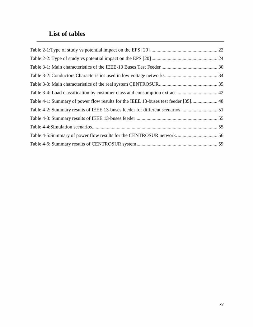
List of tables
Table 2-1:Type of study vs potential impact on the EPS [20] ...................................................... 22
Table 2-2: Type of study vs potential impact on the EPS [20] ..................................................... 24
Table 3-1: Main characteristics of the IEEE-13 Buses Test Feeder ............................................. 30
Table 3-2: Conductors Characteristics used in low voltage networks .......................................... 34
Table 3-3: Main characteristics of the real system CENTROSUR ............................................... 35
Table 3-4: Load classification by customer class and consumption extract ................................. 42
Table 4-1: Summary of power flow results for the IEEE 13-buses test feeder [35]. .................... 48
Table 4-2: Summary results of IEEE 13-buses feeder for different scenarios ............................. 51
Table 4-3: Summary results of IEEE 13-buses feeder .................................................................. 55
Table 4-4:Simulation scenarios..................................................................................................... 55
Table 4-5:Summary of power flow results for the CENTROSUR network. ................................ 56
Table 4-6: Summary results of CENTROSUR system ................................................................. 59

xvi
xvii
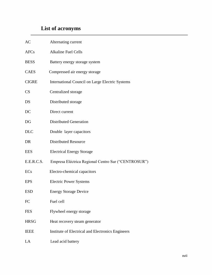
List of acronyms
AC Alternating current
AFCs Alkaline Fuel Cells
BESS Battery energy storage system
CAES Compressed air energy storage
CIGRE International Council on Large Electric Systems
CS Centralized storage
DS Distributed storage
DC Direct current
DG Distributed Generation
DLC Double layer capacitors
DR Distributed Resource
EES Electrical Energy Storage
E.E.R.C.S. Empresa Eléctrica Regional Centro Sur (“CENTROSUR”)
ECs Electro-chemical capacitors
EPS Electric Power Systems
ESD Energy Storage Device
FC Fuel cell
FES Flywheel energy storage
HRSG Heat recovery steam generator
IEEE Institute of Electrical and Electronics Engineers
LA Lead acid battery
xviii
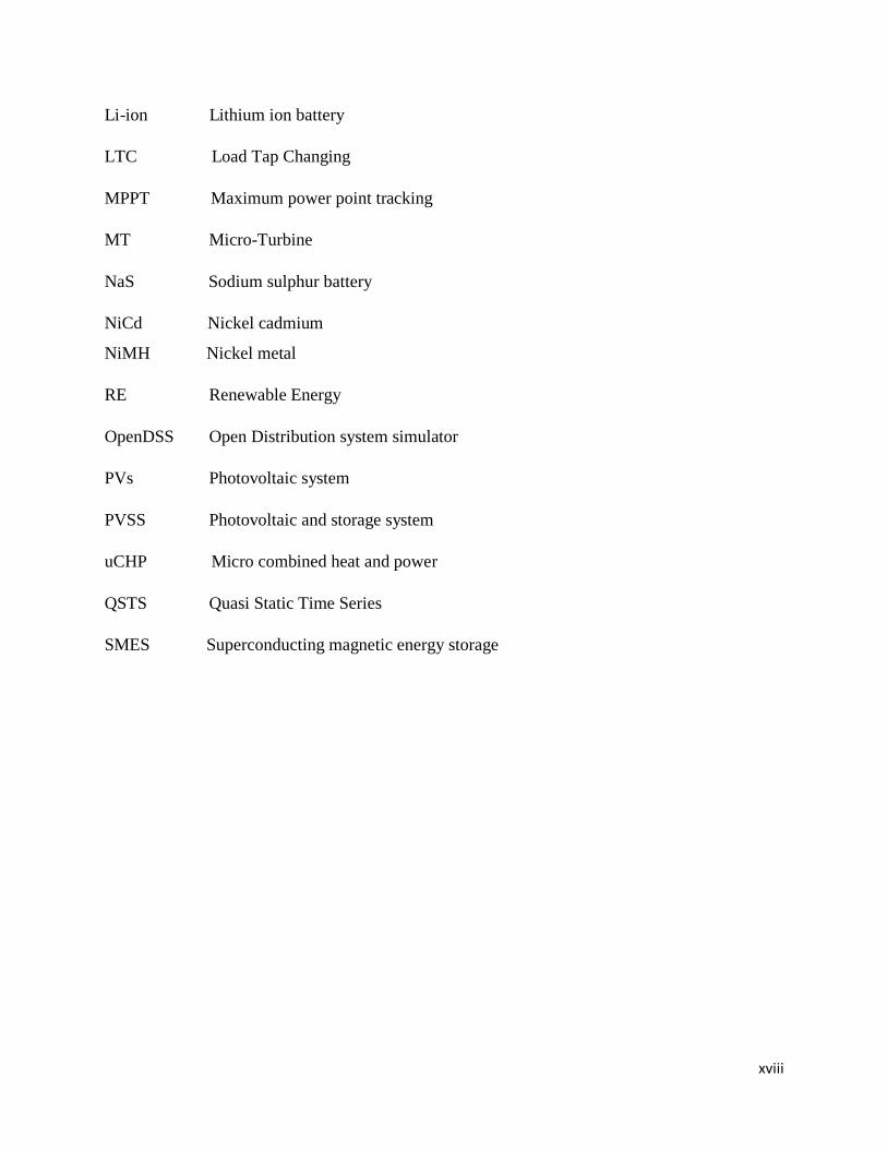
Li-ion Lithium ion battery
LTC Load Tap Changing
MPPT Maximum power point tracking
MT Micro-Turbine
NaS Sodium sulphur battery
NiCd Nickel cadmium
NiMH Nickel metal
RE Renewable Energy
OpenDSS Open Distribution system simulator
PVs Photovoltaic system
PVSS Photovoltaic and storage system
uCHP Micro combined heat and power
QSTS Quasi Static Time Series
SMES Superconducting magnetic energy storage
xix
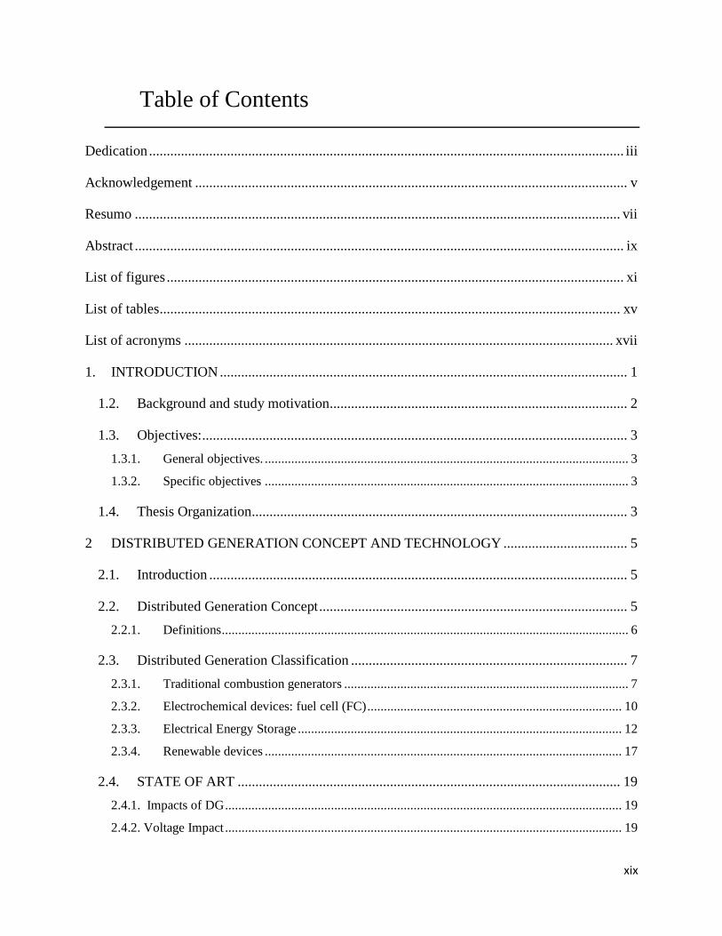
Table of Contents
Dedication ...................................................................................................................................... iii
Acknowledgement .......................................................................................................................... v
Resumo ......................................................................................................................................... vii
Abstract .......................................................................................................................................... ix
List of figures ................................................................................................................................. xi
List of tables .................................................................................................................................. xv
List of acronyms ......................................................................................................................... xvii
1. INTRODUCTION ................................................................................................................... 1
1.2. Background and study motivation.................................................................................... 2
1.3. Objectives: ........................................................................................................................ 3
1.3.1. General objectives. .............................................................................................................. 3
1.3.2. Specific objectives .............................................................................................................. 3
1.4. Thesis Organization.......................................................................................................... 3
2 DISTRIBUTED GENERATION CONCEPT AND TECHNOLOGY ................................... 5
2.1. Introduction ...................................................................................................................... 5
2.2. Distributed Generation Concept ....................................................................................... 5
2.2.1. Definitions ........................................................................................................................... 6
2.3. Distributed Generation Classification .............................................................................. 7
2.3.1. Traditional combustion generators ...................................................................................... 7
2.3.2. Electrochemical devices: fuel cell (FC) ............................................................................. 10
2.3.3. Electrical Energy Storage .................................................................................................. 12
2.3.4. Renewable devices ............................................................................................................ 17
2.4. STATE OF ART ............................................................................................................ 19
2.4.1. Impacts of DG ........................................................................................................................ 19
2.4.2. Voltage Impact ........................................................................................................................ 19
xx
2.4.3. Impact on Electric Losses ....................................................................................................... 20
2.5. IEEE standard 1547-7 .................................................................................................... 21
2.5.1. Conventional distribution studies ...................................................................................... 21
2.5.2. Special system impact studies ........................................................................................... 24
3. METODOLOGY ................................................................................................................... 27
3.1. Introduction .................................................................................................................... 27
3.2. Software OpenDSS ........................................................................................................ 27
3.3. Methodology .................................................................................................................. 28
3.3.1. Overview ........................................................................................................................... 29
3.4. LOW VOLTAGE MODELS AND CREATING LOAD PROFILES ........................... 29
3.4.1. IEEE 13-Buses Test Feeder ............................................................................................... 30
3.4.2. Real Distribution Test System (CENTROSUR) ................................................................ 31
3.5. TYPES OF ANALYSIS ................................................................................................. 36
3.5.1. Single Power Flow Analysis ............................................................................................. 36
3.5.2. QSTS Time-Series Power Flow Analysis .......................................................................... 36
3.6. TIME-SERIES DATASETS .......................................................................................... 37
3.6.1. Load Curves ...................................................................................................................... 37
3.6.2. Irradiance Curves .............................................................................................................. 38
3.7. PV SYSTEM MODEL ................................................................................................... 39
3.8. Storage element .............................................................................................................. 40
3.9. LOAD ALLOCATION .................................................................................................. 41
4. SIMULATIONS AND TEST RESULTS.............................................................................. 47
4.2. IEEE 13 BUSES SNAPSHOT SIMULATION ............................................................. 47
4.2.1. Impacts of DG on IEEE 13-buses voltages ....................................................................... 49
4.2.2. Impacts of DG on IEEE 13 buses losses............................................................................ 51
4.3. IEEE 13-BUSES QSTS SIMULATION ........................................................................ 51
4.1. Introduction .................................................................................................................... 51
4.1.1. Impacts of DG on IEEE 13-buses voltages ....................................................................... 52
xxi
4.1.2. Impacts of DG on IEEE 13 buses losses............................................................................ 54
4.2. CENTROSUR REAL SYSTEM (SNAPSHOT SIMULATION) .................................. 55
4.2.1. Impacts of DG on CENTROSUR network voltages .......................................................... 57
4.2.2. Impact of DG on CENTROSUR network losses ............................................................... 59
4.3. CENTROSUR NETWORK QSTS SOLUTION ........................................................... 60
4.3.1. CASE 1: PV ...................................................................................................................... 60
4.3.2. CASE 2: PVs integrated with Storage systems (BESS) ..................................................... 65
4.3.3. CASE 3: PVs Integrated with storage system and induction cookers ................................ 70
5. CONCLUSIONS: .................................................................................................................. 75
FUTURE WORKS........................................................................................................................ 77
PUBLICATIONS .......................................................................................................................... 78
BIBLIOGRAPHY: ........................................................................................................................ 79
APPENDIX A ............................................................................................................................... 82
ANEXO B ..................................................................................................................................... 87

xxii
1
1. INTRODUCTION
The worldwide concern about climate change on our planet is an indisputable fact. The energy
sector is one of the main generators of greenhouse gases. The use of fossil-based energy resources
causes a large emission of greenhouse gases, which contributes to environmental problems.
Population growth increases day by day promoting the increase of electricity demand that leads to
more contamination. In order to fulfill the need for more electricity, one of the solutions is to build
large power plants. However, nowadays another solution can be the use of both renewable and
non-renewable sources of energy as electric power generation within distribution networks or on
the customer side of the network, which is known as Distributed Generation (DG).
In this context, in recent times there has been a strong impetus for the development and use of
different technologies of small-scale generation, particularly those related to Renewable Energy
(RE). DGs can be defined as the concept of small sizes electric power generation units (several
kW to a few MW) connected to distribution network. The primary source of energy for these
generators can be the traditional non-renewable sources, such as gas, or the renewable sources,
such as wind, solar, hydro, and biomass. These generators can be connected either to the medium
voltage or low voltage sections of the electric grid. Usually, they are connected near the load
centers or the low voltage networks.
In addition to the integration of distributed generation points, storage systems are also being
implemented, which together are causing traditional (passive) networks to evolve into active
networks or smart-grids, in which the final consumer can be a generator or consumer. DG
alternatives, such as wind and solar, depend on wind speed and solar radiation respectively, which
makes the output power not always constant over time. Due to the fluctuation of the wind and the
variability in the solar radiation, energy storage becomes necessary for storing electrical energy.
Similarly, to conventional or renewable energy, an energy storage unit can be connected to the
distribution, sub-transmission or transmission system.
Once stored, the energy can be used during periods of high demand or when DG’s is null. All these
changes require an effort from the electricity companies to solve problems that are related to the
massive integration of DG, which means that the distribution networks are modified and have the
flexibility to guarantee the continuity and quality of service.
2
The use of DG and storage systems helps solving some of the world's problems like shortage of
energy. However, the implementation of these dispersed sources brings advantages and
disadvantages, depending especially on the correct location and capacity of generation. Dispersed
sources could change the normal operation of a common electrical power system, so the impact on
planning, control, protection and operation of the distribution system is an important issue and
should be analyzed.
This thesis discusses generally DG and the impacts of DG with energy storage on power
distribution systems considering steady state conditions.
1.2. Background and study motivation
The introduction of DG and storage systems creates a set of technical and economic challenges in
the power system. The motivation of this thesis is to study, analyze and contribute to the knowledge
of the potential impact of this technology on distribution systems.
The introduction of DG and storage systems in the distribution system can significantly modify
consumers’ power flows and voltage levels, leading to important technical issues that must be
considered when making these connections. Therefore, it is important to consider the random
establishment of DG and storage systems in distribution systems, which could bring problems in
the reliability, safety and quality of supply in the distribution network.
The Ecuadorian government, through the energy department, is implementing a program called
“towards a new energy matrix” which consists of the implementation of new renewable
technologies to produce electricity. This program considers incentive policies so that users can
generate energy through renewable resources, for self-consumption or to injected into the grid for
profit.
On the other hand, distribution networks were not designed to transport energy from the customer
to the grid. Because of this, electricity distribution utilities are carrying out studies to find out what
network parameters are affected when a customer decides to connect generation to the grid.
3
1.3. Objectives:
1.3.1. General objectives.
The general objectives of this thesis are the integration of DG and storage systems into power
distribution systems and the analysis of the its impact on the behavior of the networks considering
the characterization of different exploration scenarios.
1.3.2. Specific objectives
Analysis of the behavior of a standard IEEE distribution system before and after the
inclusion of DG and storage energy in steady state;
Analysis of a real network of the CENTROSUR Utility - Ecuador;
1.4. Thesis Organization
This thesis is composed of five chapters:
• In Chapter 1, introduction, background and motivation are described. The objectives are
also presented.
• Chapter 2 gives a brief overview of DG technologies. The literature review of modelling
distribution systems and the impacts of DG into the grid are also presented.
• Chapter 3 gives a brief description of the software used in this thesis. The Modeling of
utility distribution feeder and types of power flow analysis are also discussed.
• In Chapter 4, different scenarios of DG penetration along two feeders are proposed for both
test systems. For both systems, voltage deviation and losses through the circuit are
presented and discussed for each scenario and for two solution modes.
• Chapter 5, the last chapter provides the conclusions and recommendations in detail.

4
5
2 DISTRIBUTED GENERATION CONCEPT AND
TECHNOLOGY
2.1. Introduction
In this chapter, definitions of DG as well as storage systems are given. Types of DG technology
are presented.
2.2. Distributed Generation Concept
DG is a concept that existed years before. In the olden days, energy was provided by steam,
hydraulics, direct heating and cooling and light and the energy was produced near the device.
These happened until electricity was introduced as an alternative for the commercial purposes.
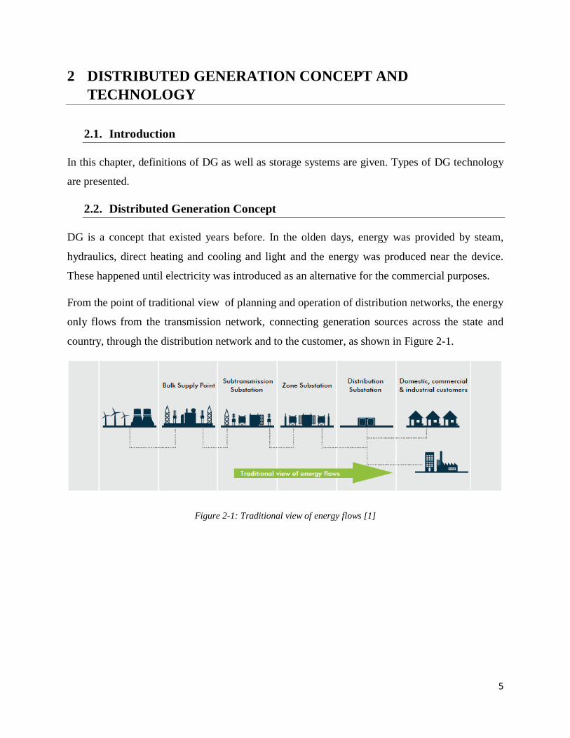
From the point of traditional view of planning and operation of distribution networks, the energy
only flows from the transmission network, connecting generation sources across the state and
country, through the distribution network and to the customer, as shown in Figure 2-1.
Figure 2-1: Traditional view of energy flows [1]
6
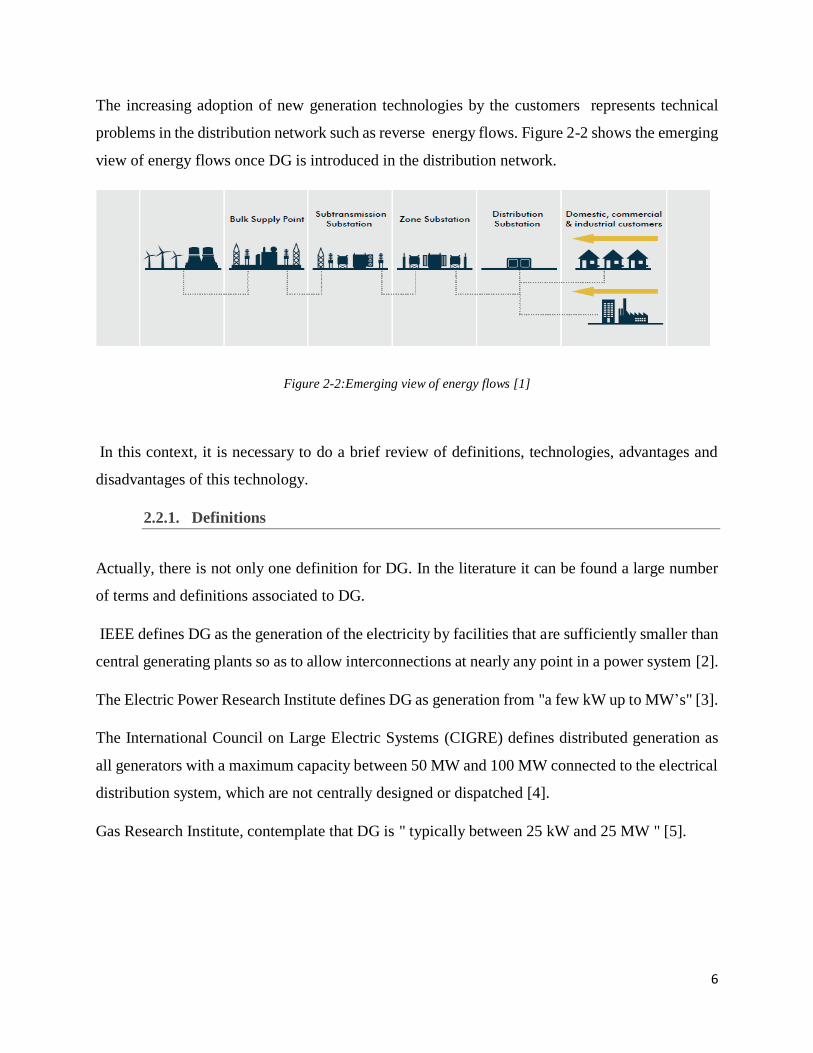
The increasing adoption of new generation technologies by the customers represents technical
problems in the distribution network such as reverse energy flows. Figure 2-2 shows the emerging
view of energy flows once DG is introduced in the distribution network.
Figure 2-2:Emerging view of energy flows [1]
In this context, it is necessary to do a brief review of definitions, technologies, advantages and
disadvantages of this technology.
2.2.1. Definitions
Actually, there is not only one definition for DG. In the literature it can be found a large number
of terms and definitions associated to DG.
IEEE defines DG as the generation of the electricity by facilities that are sufficiently smaller than
central generating plants so as to allow interconnections at nearly any point in a power system [2].
The Electric Power Research Institute defines DG as generation from "a few kW up to MW’s" [3].
The International Council on Large Electric Systems (CIGRE) defines distributed generation as
all generators with a maximum capacity between 50 MW and 100 MW connected to the electrical
distribution system, which are not centrally designed or dispatched [4].
Gas Research Institute, contemplate that DG is " typically between 25 kW and 25 MW " [5].
7
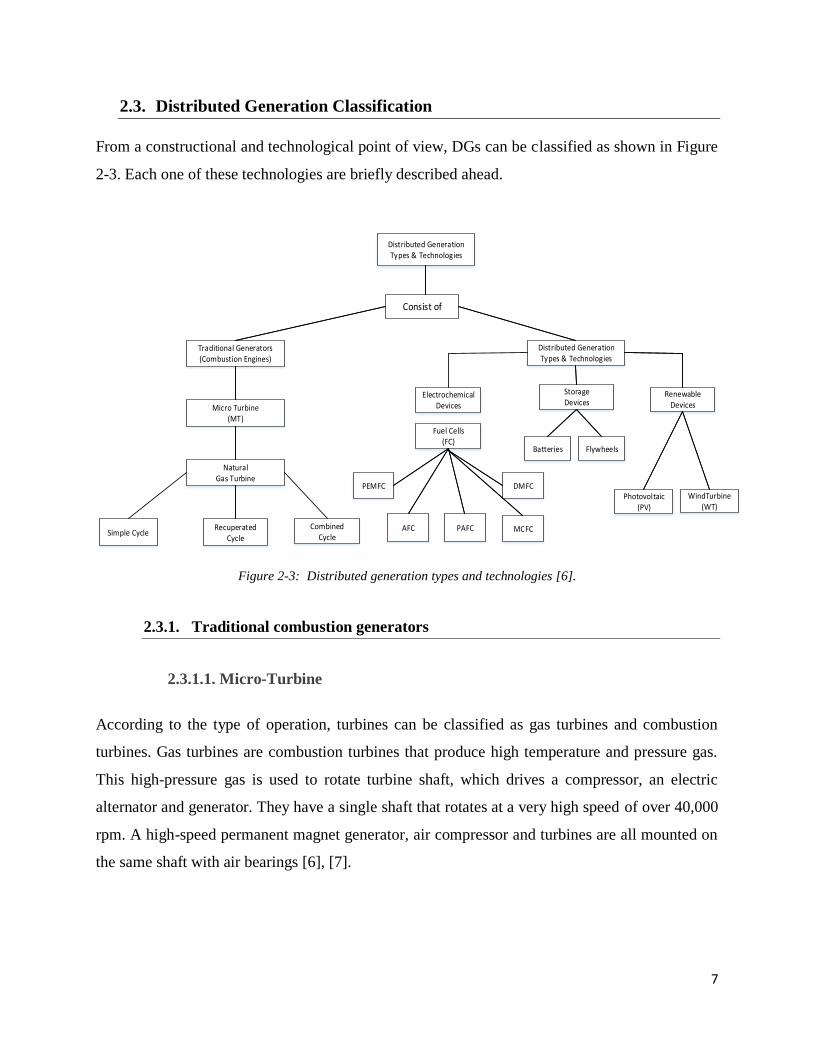
2.3. Distributed Generation Classification
From a constructional and technological point of view, DGs can be classified as shown in Figure
2-3. Each one of these technologies are briefly described ahead.
Distributed GenerationTypes & Technologies
Traditional Generators(Combustion Engines)
Distributed GenerationTypes & Technologies
Consist of
Micro Turbine(MT)
Natural Gas Turbine
Simple CycleRecuperated
Cycle
CombinedCycle
ElectrochemicalDevices
Fuel Cells(FC)
PEMFC
AFC PAFC MCFC
DMFC
StorageDevices
Batteries Flywheels
RenewableDevices
Photovoltaic(PV)
WindTurbine(WT)
Figure 2-3: Distributed generation types and technologies [6].
2.3.1. Traditional combustion generators
2.3.1.1. Micro-Turbine
According to the type of operation, turbines can be classified as gas turbines and combustion
turbines. Gas turbines are combustion turbines that produce high temperature and pressure gas.
This high-pressure gas is used to rotate turbine shaft, which drives a compressor, an electric
alternator and generator. They have a single shaft that rotates at a very high speed of over 40,000
rpm. A high-speed permanent magnet generator, air compressor and turbines are all mounted on
the same shaft with air bearings [6], [7].
8
These kinds of turbines are small combustions turbines with power outputs from 25 kW to 500
kW. This kind of technology has advantages that includes lower emission, high efficiency and
compact size. Therefore, it is expected them to have a bright future.
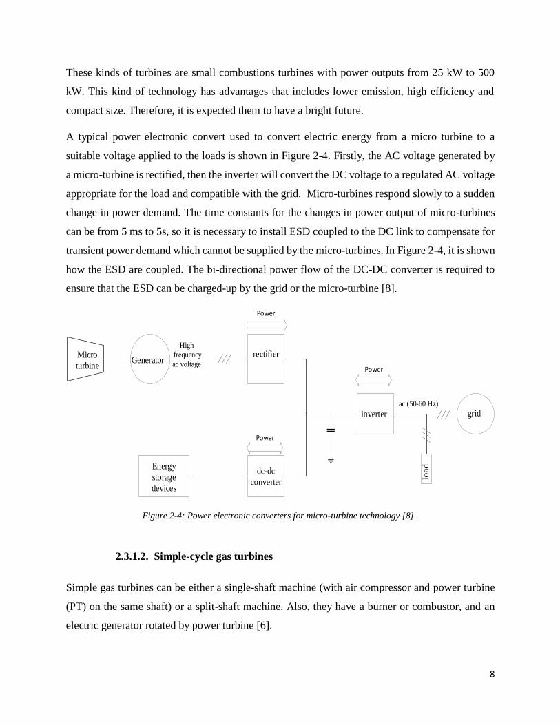
A typical power electronic convert used to convert electric energy from a micro turbine to a
suitable voltage applied to the loads is shown in Figure 2-4. Firstly, the AC voltage generated by
a micro-turbine is rectified, then the inverter will convert the DC voltage to a regulated AC voltage
appropriate for the load and compatible with the grid. Micro-turbines respond slowly to a sudden
change in power demand. The time constants for the changes in power output of micro-turbines
can be from 5 ms to 5s, so it is necessary to install ESD coupled to the DC link to compensate for
transient power demand which cannot be supplied by the micro-turbines. In Figure 2-4, it is shown
how the ESD are coupled. The bi-directional power flow of the DC-DC converter is required to
ensure that the ESD can be charged-up by the grid or the micro-turbine [8].
Generatorrectifier
High
frequency
ac voltage
dc-dc
converter
Energy
storage
devices
Power
inverter
Power
grid
load
ac (50-60 Hz)
Power
Micro
turbine
Figure 2-4: Power electronic converters for micro-turbine technology [8] .
2.3.1.2. Simple-cycle gas turbines
Simple gas turbines can be either a single-shaft machine (with air compressor and power turbine
(PT) on the same shaft) or a split-shaft machine. Also, they have a burner or combustor, and an
electric generator rotated by power turbine [6].
9
2.3.1.3. Recuperated gas turbines
These turbines have a special heat exchanger (a recuperator), which uses the output exhaust
thermal energy to preheat compressed air in its pass to the burner to increase the turbine electrical
efficiency.
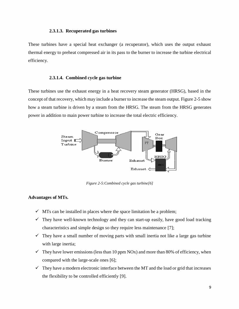
2.3.1.4. Combined cycle gas turbine
These turbines use the exhaust energy in a heat recovery steam generator (HRSG), based in the
concept of that recovery, which may include a burner to increase the steam output. Figure 2-5 show
how a steam turbine is driven by a steam from the HRSG. The steam from the HRSG generates
power in addition to main power turbine to increase the total electric efficiency.
Figure 2-5:Combined cycle gas turbine[6]
Advantages of MTs.
MTs can be installed in places where the space limitation be a problem;
They have well-known technology and they can start-up easily, have good load tracking
characteristics and simple design so they require less maintenance [7];
They have a small number of moving parts with small inertia not like a large gas turbine
with large inertia;
They have lower emissions (less than 10 ppm NOx) and more than 80% of efficiency, when
compared with the large-scale ones [6];
They have a modern electronic interface between the MT and the load or grid that increases
the flexibility to be controlled efficiently [9].
10
2.3.2. Electrochemical devices: fuel cell (FC)
FCs are devices that use electrodes and electrolytic materials to accomplish the electrochemical
production of electricity. They do not store chemical energy, but rather, convert the chemical
energy of a fuel to electricity. Unlike batteries, FC does not need to be charged for the consumed
materials during the electrochemical process since these materials are continuously supplied [10].
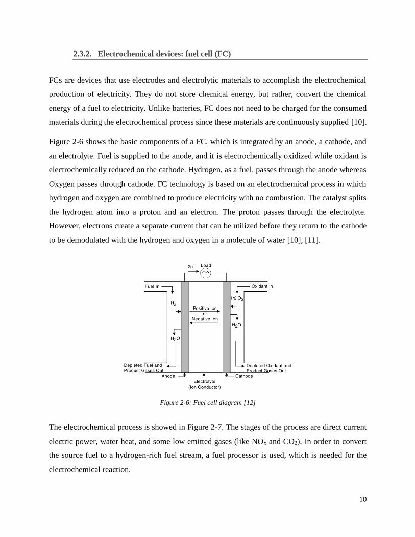
Figure 2-6 shows the basic components of a FC, which is integrated by an anode, a cathode, and
an electrolyte. Fuel is supplied to the anode, and it is electrochemically oxidized while oxidant is
electrochemically reduced on the cathode. Hydrogen, as a fuel, passes through the anode whereas
Oxygen passes through cathode. FC technology is based on an electrochemical process in which
hydrogen and oxygen are combined to produce electricity with no combustion. The catalyst splits
the hydrogen atom into a proton and an electron. The proton passes through the electrolyte.
However, electrons create a separate current that can be utilized before they return to the cathode
to be demodulated with the hydrogen and oxygen in a molecule of water [10], [11].
Figure 2-6: Fuel cell diagram [12]
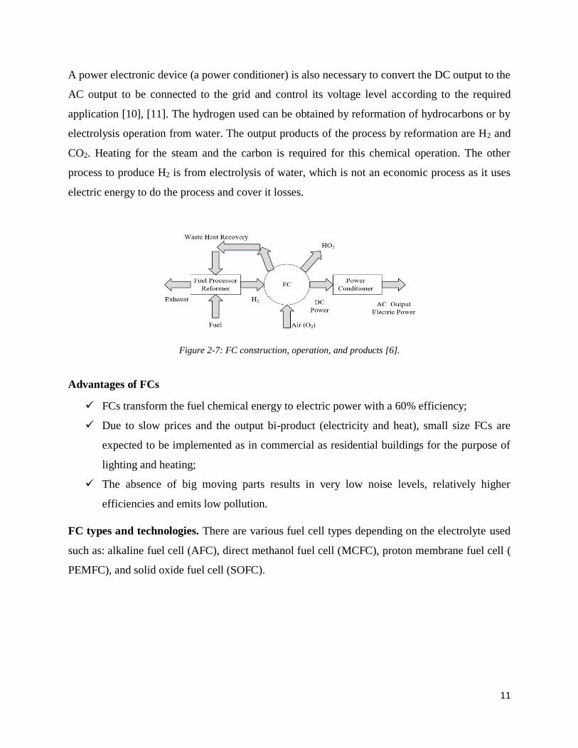
The electrochemical process is showed in Figure 2-7. The stages of the process are direct current
electric power, water heat, and some low emitted gases (like NOx and CO2). In order to convert
the source fuel to a hydrogen-rich fuel stream, a fuel processor is used, which is needed for the
electrochemical reaction.
11
A power electronic device (a power conditioner) is also necessary to convert the DC output to the
AC output to be connected to the grid and control its voltage level according to the required
application [10], [11]. The hydrogen used can be obtained by reformation of hydrocarbons or by
electrolysis operation from water. The output products of the process by reformation are H2 and
CO2. Heating for the steam and the carbon is required for this chemical operation. The other
process to produce H2 is from electrolysis of water, which is not an economic process as it uses
electric energy to do the process and cover it losses.
Figure 2-7: FC construction, operation, and products [6].
Advantages of FCs
FCs transform the fuel chemical energy to electric power with a 60% efficiency;
Due to slow prices and the output bi-product (electricity and heat), small size FCs are
expected to be implemented as in commercial as residential buildings for the purpose of
lighting and heating;
The absence of big moving parts results in very low noise levels, relatively higher
efficiencies and emits low pollution.
FC types and technologies. There are various fuel cell types depending on the electrolyte used
such as: alkaline fuel cell (AFC), direct methanol fuel cell (MCFC), proton membrane fuel cell (
PEMFC), and solid oxide fuel cell (SOFC).
12
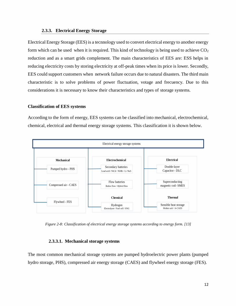
2.3.3. Electrical Energy Storage
Electrical Energy Storage (EES) is a tecnnology used to convert electrical energy to another energy
form which can be used when it is required. This kind of technology is being used to achieve CO2
reduction and as a smart grids complement. The main characteristics of EES are: ESS helps in
reducing electricity costs by storing electricity at off-peak times when its price is lower. Secondly,
EES could support customers when network failure occurs due to natural disasters. The third main
characteristic is to solve problems of power fluctuation, votage and frecuency. Due to this
considerations it is necessary to know their characteristics and types of storage systems.
Classification of EES systems
According to the form of energy, EES systems can be classified into mechanical, electrochemical,
chemical, electrical and thermal energy storage systems. This classification it is shown below.
Electrical energy storage systems
Pumped hydro - PHS
Compressed air - CAES
Flywheel - FES
Mechanical
Secondary batteries
Lead acid / NiCd / NiMh / Li /NaS
Flow batteries
Redox flow / Hybrid flow
HydrogenElectrolyser / Fuel cell / SNG
Electrochemical
Chemical
Double-layer
Capacitor - DLC
Superconducting
magnetic coil- SMES
Sensible heat storageMolten salt / A-CAES
Electrical
Thermal
Figure 2-8: Classification of electrical energy storage systems according to energy form. [13]
2.3.3.1. Mechanical storage systems
The most common mechanical storage systems are pumped hydroelectric power plants (pumped
hydro storage, PHS), compressed air energy storage (CAES) and flywheel energy storage (FES).
13
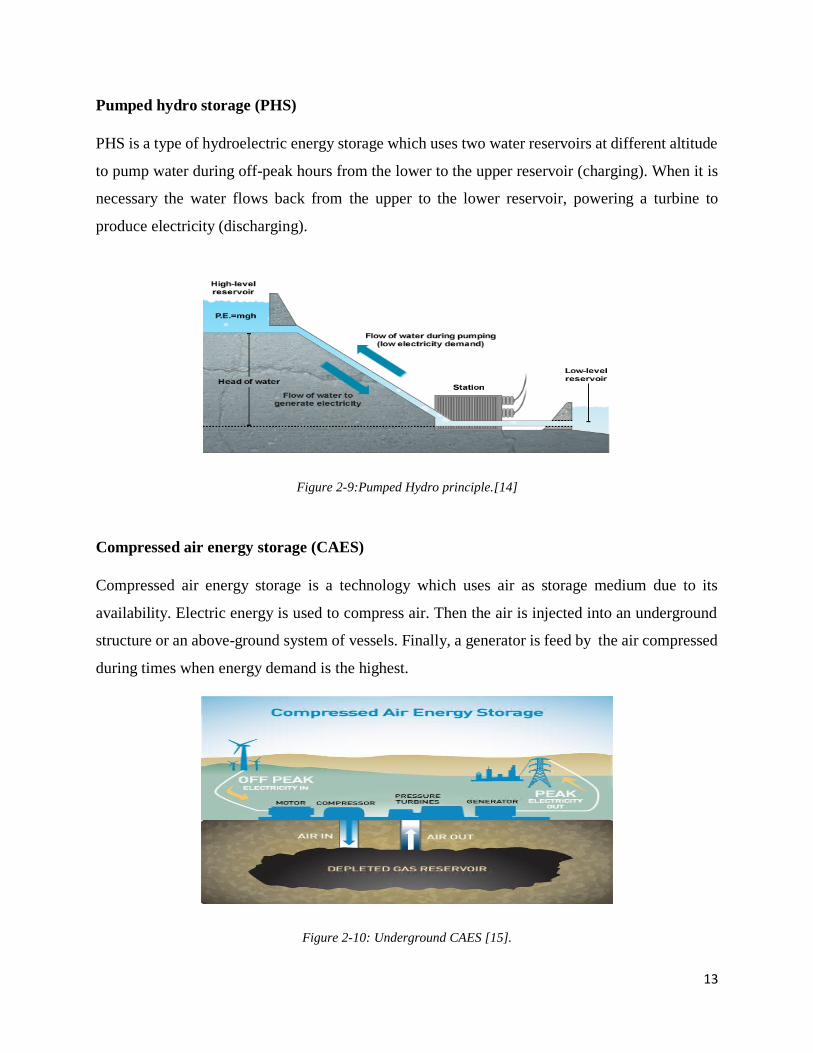
Pumped hydro storage (PHS)
PHS is a type of hydroelectric energy storage which uses two water reservoirs at different altitude
to pump water during off-peak hours from the lower to the upper reservoir (charging). When it is
necessary the water flows back from the upper to the lower reservoir, powering a turbine to
produce electricity (discharging).
Figure 2-9:Pumped Hydro principle.[14]
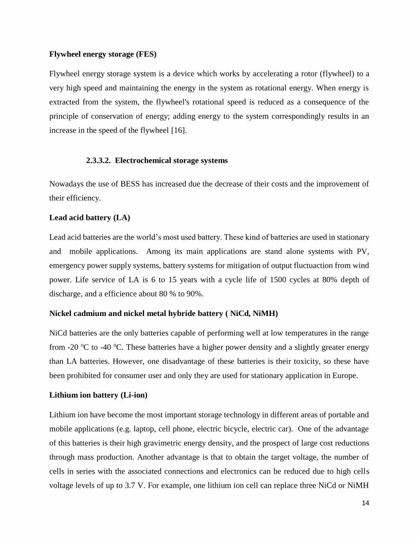
Compressed air energy storage (CAES)
Compressed air energy storage is a technology which uses air as storage medium due to its
availability. Electric energy is used to compress air. Then the air is injected into an underground
structure or an above-ground system of vessels. Finally, a generator is feed by the air compressed
during times when energy demand is the highest.
Figure 2-10: Underground CAES [15].
14
Flywheel energy storage (FES)
Flywheel energy storage system is a device which works by accelerating a rotor (flywheel) to a
very high speed and maintaining the energy in the system as rotational energy. When energy is
extracted from the system, the flywheel's rotational speed is reduced as a consequence of the
principle of conservation of energy; adding energy to the system correspondingly results in an
increase in the speed of the flywheel [16].
2.3.3.2. Electrochemical storage systems
Nowadays the use of BESS has increased due the decrease of their costs and the improvement of
their efficiency.
Lead acid battery (LA)
Lead acid batteries are the world’s most used battery. These kind of batteries are used in stationary
and mobile applications. Among its main applications are stand alone systems with PV,
emergency power supply systems, battery systems for mitigation of output fluctuaction from wind
power. Life service of LA is 6 to 15 years with a cycle life of 1500 cycles at 80% depth of
discharge, and a efficience about 80 % to 90%.
Nickel cadmium and nickel metal hybride battery ( NiCd, NiMH)
NiCd batteries are the only batteries capable of performing well at low temperatures in the range
from -20 oC to -40 oC. These batteries have a higher power density and a slightly greater energy
than LA batteries. However, one disadvantage of these batteries is their toxicity, so these have
been prohibited for consumer user and only they are used for stationary application in Europe.
Lithium ion battery (Li-ion)
Lithium ion have become the most important storage technology in different areas of portable and
mobile applications (e.g. laptop, cell phone, electric bicycle, electric car). One of the advantage
of this batteries is their high gravimetric energy density, and the prospect of large cost reductions
through mass production. Another advantage is that to obtain the target voltage, the number of
cells in series with the associated connections and electronics can be reduced due to high cells
voltage levels of up to 3.7 V. For example, one lithium ion cell can replace three NiCd or NiMH
15
cells which have a cell voltage of only 1.2 Volts. The main drawback is the cost which is USD
600/kWh due to special packaging an internal overcharge protection circuits [13].
Sodium sulphur battery (NaS)
Sodium sulphur batteries consist of liquid (molten) sulphur at the positive electrode and liquid
(molten) sodium at the negative electrode; the active materials are separated by a solid beta
alumina ceramic electrolyte. The battery temperature is kept between 300 °C and 350 °C to keep
the electrodes molten. These batteries have a discharge time of 6. hours to 7.2 hours, and a life
cycles around 4500 cycles. Their efficiency is about 75% and commonly are used in combined
power quality and time shift applications with energy density [13].
Flow batteries
A flow battery is a rechargable battery that storage energy in one or more electroactive species
which are dissolved in liquid electrolytes. The electrolytes are stored externally in tanks and
pumped through the electrochemical cell that converts chemical energy directly to electricity and
vice versa. The power is defined by the size and design of the electrochemical cell whereas the
energy depends on the size of the tanks. Althought these batteries were developed by NASA in the
70s as EES for long term space flights, flow batteries are not commonly being used.
2.3.3.3. Electrical storage sytems
Double – layer capacitors (DLC)
Electro-chemical capacitors (ECs) are known by different names as ultra-capacitors, DLC or super
capacitor. All the name used before refer to a capacitor, which stores electrical energy in the
interface between an electrolyte and a solid electrode. The advantages of this technology are
durability, high reability, long lifetime, and operation over a wide temperature. Also, two of the
main features are the possibility of very fast charges and discharges due to low inner resistance,
and the really high capacitance value, typically in order of many thousand farads. DLC technology
where a large number of short charge/ discharge used in applications with a large number being
16
required. Due to the investment costs, DLC are not suitable for the energy storage over long time
periods.
Superconducting magnetic energy storage (SMES)
Superconducting magnetic energy storage (SMES) systems work according to an electrodynamic
principle. This systems storage energy in the magnetic field created by the flow of direct current
in a superconducting coil, which is kept below its superconducting critical temperature. 100 years
ago at the discovery of superconductivity a temperature of about 4 °K was needed. Much research
and some luck has now produced superconducting materials with higher critical temperatures.
Today materials are available which can function at around 100 °K. The main parts of this storage
system are a coil made of superconducting material, power conditioning and a cryogenically
cooled refrigirator. Due to high cost of superconducting wire and refrigeration requirerments,
SMES is only used for short duration energy storage.
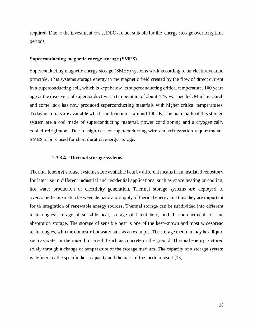
2.3.3.4. Thermal storage systems
Thermal (energy) storage systems store available heat by different means in an insulated repository
for later use in different industrial and residential applications, such as space heating or cooling,
hot water production or electricity generation. Thermal storage systems are deployed to
overcomethe mismatch between demand and supply of thermal energy and thus they are important
for th integration of renewable energy sources. Thermal storage can be subdivided into different
technologies: storage of sensible heat, storage of latent heat, and thermo-chemical ad- and
absorption storage. The storage of sensible heat is one of the best-known and most widespread
technologies, with the domestic hot water tank as an example. The storage medium may be a liquid
such as water or thermo-oil, or a solid such as concrete or the ground. Thermal energy is stored
solely through a change of temperature of the storage medium. The capacity of a storage system
is defined by the specific heat capacity and themass of the medium used [13].
17
2.3.4. Renewable devices
RE is energy generated from natural resources such as sunlight, wind and water. Some types of
RE are discussed below.
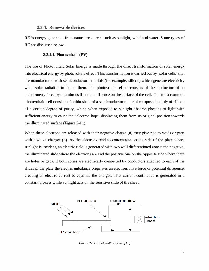
2.3.4.1. Photovoltaic (PV)
The use of Photovoltaic Solar Energy is made through the direct transformation of solar energy
into electrical energy by photovoltaic effect. This transformation is carried out by "solar cells" that
are manufactured with semiconductor materials (for example, silicon) which generate electricity
when solar radiation influence them. The photovoltaic effect consists of the production of an
electrometry force by a luminous flux that influence on the surface of the cell. The most common
photovoltaic cell consists of a thin sheet of a semiconductor material composed mainly of silicon
of a certain degree of purity, which when exposed to sunlight absorbs photons of light with
sufficient energy to cause the "electron hop", displacing them from its original position towards
the illuminated surface (Figure 2-11).
When these electrons are released with their negative charge (n) they give rise to voids or gaps
with positive charges (p). As the electrons tend to concentrate on the side of the plate where
sunlight is incident, an electric field is generated with two well differentiated zones: the negative,
the illuminated slide where the electrons are and the positive one on the opposite side where there
are holes or gaps. If both zones are electrically connected by conductors attached to each of the
slides of the plate the electric unbalance originates an electromotive force or potential difference,
creating an electric current to equalize the charges. That current continuous is generated in a
constant process while sunlight acts on the sensitive slide of the sheet.
Figure 2-11: Photovoltaic panel [17]
18
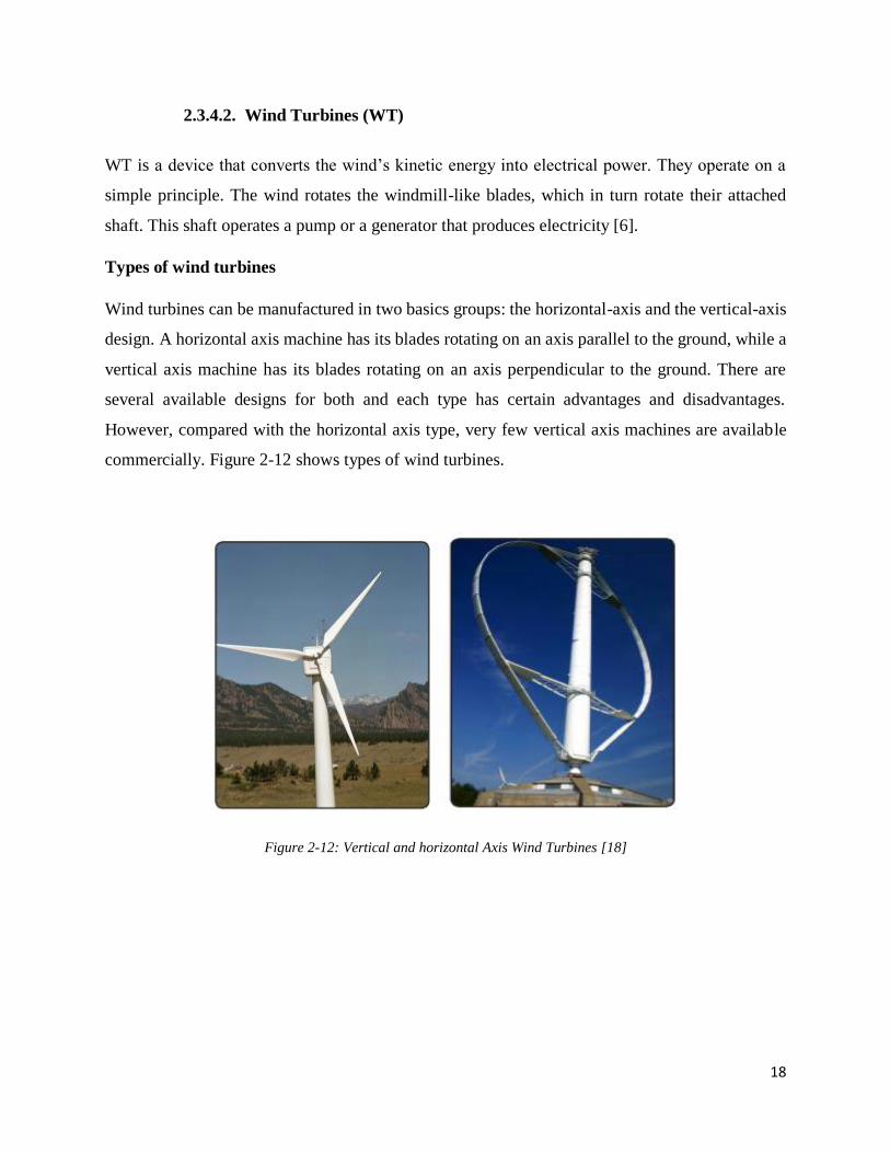
2.3.4.2. Wind Turbines (WT)
WT is a device that converts the wind’s kinetic energy into electrical power. They operate on a
simple principle. The wind rotates the windmill-like blades, which in turn rotate their attached
shaft. This shaft operates a pump or a generator that produces electricity [6].
Types of wind turbines
Wind turbines can be manufactured in two basics groups: the horizontal-axis and the vertical-axis
design. A horizontal axis machine has its blades rotating on an axis parallel to the ground, while a
vertical axis machine has its blades rotating on an axis perpendicular to the ground. There are
several available designs for both and each type has certain advantages and disadvantages.
However, compared with the horizontal axis type, very few vertical axis machines are available
commercially. Figure 2-12 shows types of wind turbines.
Figure 2-12: Vertical and horizontal Axis Wind Turbines [18]
19
2.4. STATE OF ART
This section presents the state of art related to the impact of DG on electric power networks. In the
current scientific literature, there are several published work concerning the integration of DG into
distribution systems. However, the most representative works associated with each of the factors
involved in formulating the problem and determining variables in the evaluation of the penetration
of DG are described below.
2.4.1. Impacts of DG
Impacts of DG on electrical energy systems are inevitable, and therefore control requires the
efforts of generation companies and users. The implementation of DG can be reflected in
phenomena such as: bus voltage, harmonics, power losses, reliability, etc. Through the inclusion
of DG, the power flow can be bidirectional and it can cause overvoltage on the distribution system.
There are some interconnection guidelines in order to connect DG to the distribution network. In
[19], rules for studying the impacts of interconnecting DG to a distribution feeder are defined. The
IEEE 15474.7 standard [20] for distributed resource interconnection provides technical criterion
and requirements for interconnecting DG resources to distribution systems.
2.4.2. Voltage Impact
In scientific literature, there are many studies which have analyzed the impact of DG on technical
parameters such as voltages, losses, capacity, reliability and power quality. For example in [21],
the impacts of utility scale PV-DG on power distribution systems is reviewed, particularly in terms
of planning and operation in steady state and dynamic conditions. One of the conclusions of this
study is the improvement of voltage profiles when DG is considered. In this study mitigation
measures such as distributed storage are also presented with the purpose of reducing the magnitude
of voltage fluctuation on the feeder analyzed [21]. In [22], a study of time series power flow
analysis for distribution connected PV generation is carried out in three real feeders and over the
IEEE 8500 node feeder. The main purpose of this study was to find out how analysis using Quasi-
static time series (QSTS) simulation and high time resolution data can quantify the impacts and
the mitigation strategies to address voltage regulation operation, and steady state voltage. In
20
reference [23] analyzed voltages problems due to DG penetration. The simulations were performed
under the worst network condition (minimum demand and maximum DG output power). Monte
Carlo method was used to allocate DG. Also in this study, was determined that a small amount of
DG can produce voltage violations while very large amounts of DG allocated with adequate
criterion do not affect the system operation. Reference [24] assesses the impact of low carbon
technologies in LV distribution systems. Firstly, a realistic 5-minute time series daily profile is
produced for photovoltaic panel, electric heat pump, electric vehicles and micro combined heat
and power units. After that, a Monte Carlo simulation is carried out for 128 real UK LV feeders.
Results for this study showed that photovoltaic (PV) panels technology produced problems in 47%
of the feeders, EHPs produced problems in 53% of the feeders and EVs produced problems in 34%
of the feeders. For uCHP no problems were found. In reference [25], the impacts of DG on voltage
regulation by Load Tap Changing (LTC) transformer were studied. That study shows that if the
LTC tap transformer control is not applied, problems of under voltages and over voltages can
occur. In [26] energy storage is used for voltage support in low voltage grids when high
photovoltaic penetration is added. Centralized storage (CS) and distributed storage (DS) are
investigated. CS is implemented by adding a single storage unit on a feeder node while DS
integrated a storage device together with PV at a feeder location.
2.4.3. Impact on Electric Losses
In [27], technical impacts of microgeneration on low voltage distribution networks are analyzed.
Impact analysis on losses demonstrates that an adequate amount of PV generation (30% PV)
decreased the daily total losses in the system while an inappropriate amount of PV (100%)
generation increased losses. In reference [28], the impact of DG of a distribution network on
voltage profile and energy losses are analyzed. The results obtained in this paper show that an
adequate location and size of DG are essential for reducing power losses and voltage profile. In
[29], a probabilistic technique for optimal allocation of PV based distributed generators to decrease
system losses is developed. In that research work are presented six cases. For the base case, without
DG, the annual energy loss is 540.967 MWh, while for case 6 when DG of 1590 kW is added the
annual energy losses were reduced to 161.721 MWh, which represents an energy and economic
saving.
21
2.5. IEEE standard 1547-7
In this section, it is presented a brief explanation of the main impact studies that should be
developed according to IEEE standard 1547-7. The IEEE standard 1547-7 is a guide which
describes criteria, scope, and extent for engineering studies of the impact on area electric power
systems of a distributed resource (DR) or aggregate distributed resource interconnected to an area
electric power distribution system [20].
In the following two tables, different conventional systems impact studies and their relationship to
potential systems impacts on the Electric Power System (EPS) area are shown. In section 1.2 of
chapter 1 it was established that the analysis of the distribution networks will be carried out in
steady state. Under this consideration, the green area painted in each one of the tables would
correspond to the proposed analysis in that section. According to this standard, the steady state
study and the quasi-static study are briefly explained in this section.
2.5.1. Conventional distribution studies
According to this standard, a large Distributed Resource (DR) could cause voltage variations,
overload, equipment misoperations, protection and coordination, and power quality issues in the
(EPS) area. Once DR is connected to the grid and if it exceeds some criteria limits, the DR should
be studied using conventional studies which are presented in Table 2-1.
22
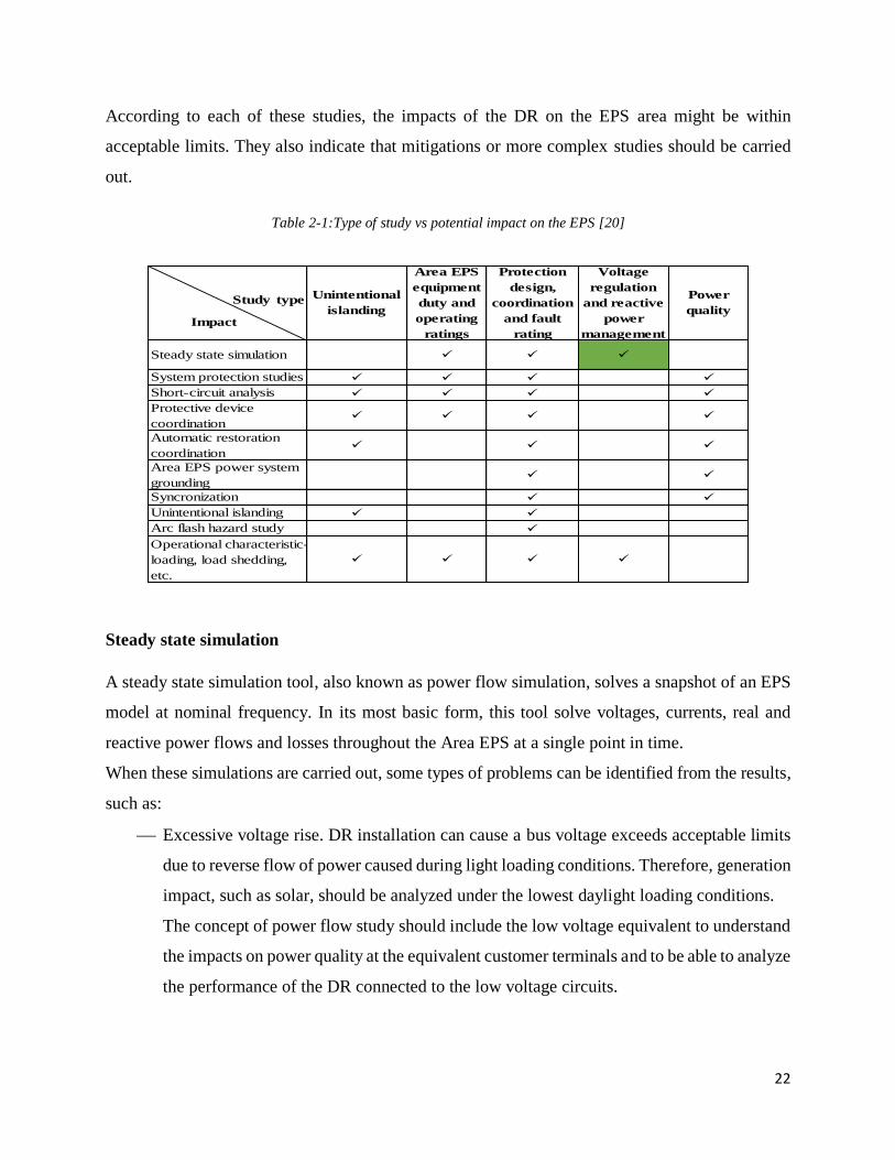
According to each of these studies, the impacts of the DR on the EPS area might be within
acceptable limits. They also indicate that mitigations or more complex studies should be carried
out.
Table 2-1:Type of study vs potential impact on the EPS [20]
Syncronization
Unintentional islanding
Arc flash hazard study
Operational characteristic-
loading, load shedding,
etc.
Automatic restoration
coordination
Area EPS power system
grounding
System protection studies
Short-circuit analysis
Protective device
coordination
Voltage
regulation
and reactive
power
management
Power
quality
Steady state simulation
Unintentional
islanding
Area EPS
equipment
duty and
operating
ratings
Protection
design,
coordination
and fault
ratingImpact
Study type
Steady state simulation
A steady state simulation tool, also known as power flow simulation, solves a snapshot of an EPS
model at nominal frequency. In its most basic form, this tool solve voltages, currents, real and
reactive power flows and losses throughout the Area EPS at a single point in time.
When these simulations are carried out, some types of problems can be identified from the results,
such as:
Excessive voltage rise. DR installation can cause a bus voltage exceeds acceptable limits
due to reverse flow of power caused during light loading conditions. Therefore, generation
impact, such as solar, should be analyzed under the lowest daylight loading conditions.
The concept of power flow study should include the low voltage equivalent to understand
the impacts on power quality at the equivalent customer terminals and to be able to analyze
the performance of the DR connected to the low voltage circuits.
23
Excessive voltage fluctuations. DR, such as wind and solar generation can cause voltage
fluctuations which can be irritating to some customers. However, circuit voltage can be
controlled through voltage regulators and capacitor banks.
Improper operation. When DR is added, it can create reverse power, which causes
improperly equipment operation. Voltage regulation equipment is designed to operate as
through power flow in only one direction from the source to the customer. Nevertheless,
the inclusion of DS could cause a reversal power flow from the customer to the source,
and in this way the equipment can wrongly adjust the voltage. This condition commonly
happens under light load condition.
Incorrect situational awareness. If large DR is installed on a circuit, circuit metering may
be analyzed to know if the reverse power flow would be identified in readings provided to
the system operators. Metering equipment should be replaced in order to capture
bidirectional flow.
Equipment overloads. If the connection of DR is larger than the local load, an
equipment overloads can be caused in the Area EPS. These overloads may occur at any
time and not only at peak conditions.
Unbalanced operation. When the DR is installed at the location of area EPS with
significant phase imbalances can cause voltage imbalance on the generator terminals.
Single phase DR installation can increase the imbalance, which in turn causes serious
impact on other devices connected to the area EPS circuits. Through a three-phase power
flow analysis tool, modeling single phase DR or three- phase DR on unbalanced circuits
can recognize the complications that may occur on the circuit. Problems can be detected
that occur in a circuit in which a single-phase DR or three-phase DR on unbalanced circuit
have been modeled.
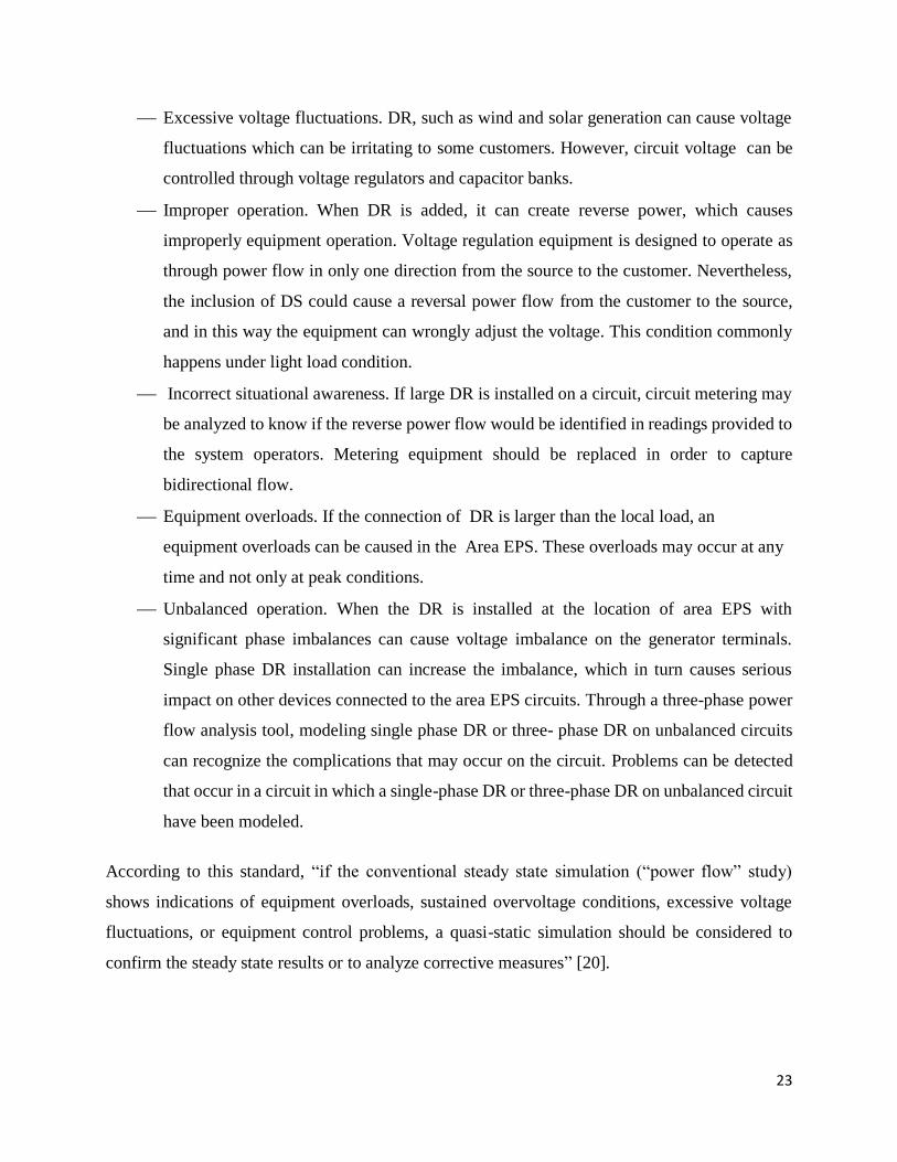
According to this standard, “if the conventional steady state simulation (“power flow” study)
shows indications of equipment overloads, sustained overvoltage conditions, excessive voltage
fluctuations, or equipment control problems, a quasi-static simulation should be considered to
confirm the steady state results or to analyze corrective measures” [20].
24
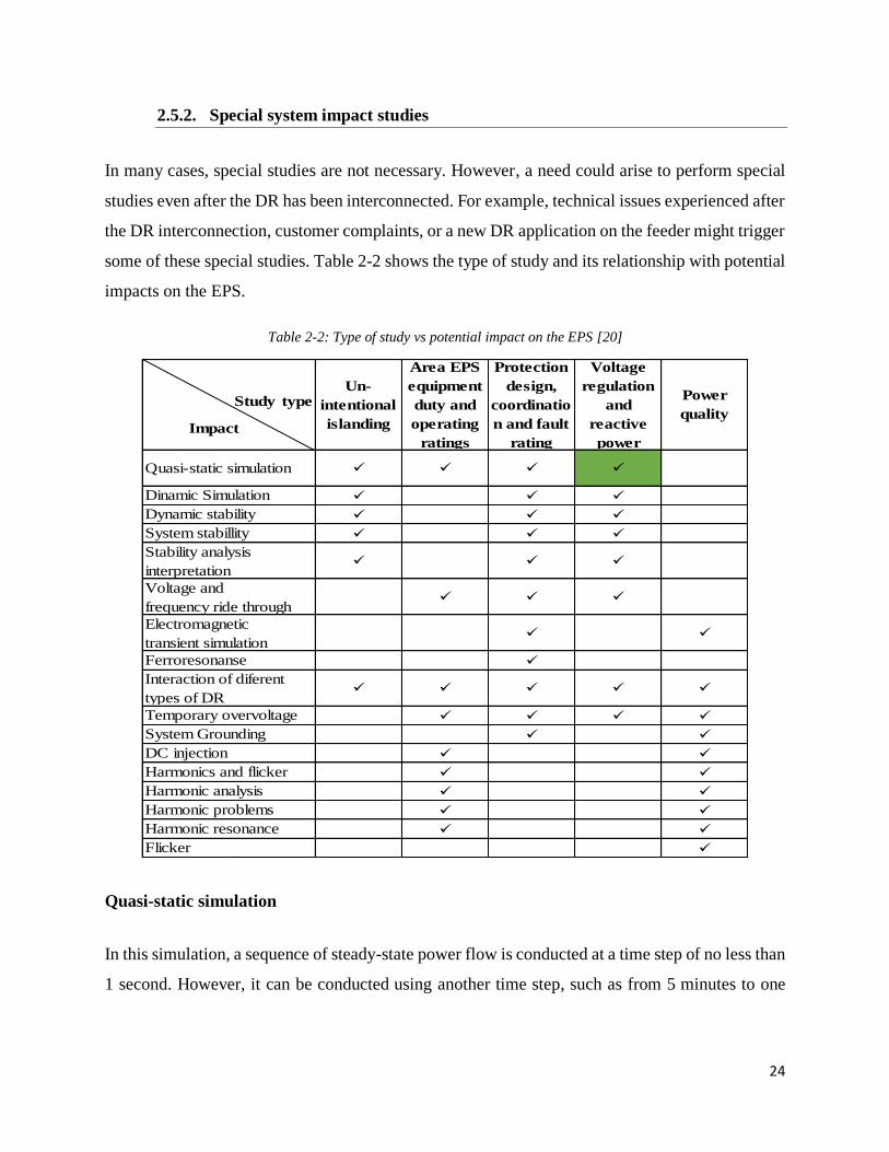
2.5.2. Special system impact studies
In many cases, special studies are not necessary. However, a need could arise to perform special
studies even after the DR has been interconnected. For example, technical issues experienced after
the DR interconnection, customer complaints, or a new DR application on the feeder might trigger
some of these special studies. Table 2-2 shows the type of study and its relationship with potential
impacts on the EPS.
Table 2-2: Type of study vs potential impact on the EPS [20]
Un-
intentional
islanding
Area EPS
equipment
duty and
operating
ratings
Protection
design,
coordinatio
n and fault
rating
Voltage
regulation
and
reactive
power
Power
quality
Quasi-static simulation
Dinamic Simulation
Dynamic stability
System stabillity
Stability analysis
interpretation
Voltage and
frequency ride through
Electromagnetic
transient simulation
Ferroresonanse
Interaction of diferent
types of DR
Harmonic problems
Harmonic resonance
Flicker
Temporary overvoltage
System Grounding
DC injection
Harmonics and flicker
Harmonic analysis
Impact
Study type
Quasi-static simulation
In this simulation, a sequence of steady-state power flow is conducted at a time step of no less than
1 second. However, it can be conducted using another time step, such as from 5 minutes to one
25
hour. Applications such as energy and loss evaluation of generation and load profiles can be carried
out under this solution mode.
As is known, solar and wind are variable resources by a quasi-static simulation, voltage fluctuation
impacts due to variable DR output can be analyzed. The impact on voltage controls can be
observed by quasi-static solution. Another advantage of this solution mode is that it can show the
impact of DR on system equipment and customers.

26
27
3. METODOLOGY
3.1. Introduction
In this chapter, an explanation of the utility feeders model and its components is presented. The
feeders were modeled using OpenDSS software. The main characteristics of lines, transformers
and customer are given in this chapter. The procedure to evaluate the DG technical impacts is also
described.
3.2. Software OpenDSS
OpenDSS is an electrical system simulation tool for electric utility distribution systems. It can be
implemented as stand-alone executable program or by the COM server DLL. At the beginning, the
program was originally developed to support DG analysis. However, it has been improved and
designed to be expandable for the future needs.
Some of the applications that have used OpenDSS are:
• Distribution Planning and Analysis
• Analysis of Distributed Generation Interconnections
• Annual Load and Generation Simulations
• Risk based Distribution Planning Studies
• Probabilistic Planning Studies
• Solar PV System Simulation
• Wind Plant Simulations
• Protection System Simulation
• Storage Modeling
• EV Impacts Simulations
• Harmonic and Interharmonic Distortion Analysis
• Development of IEEE Test feeder cases
28
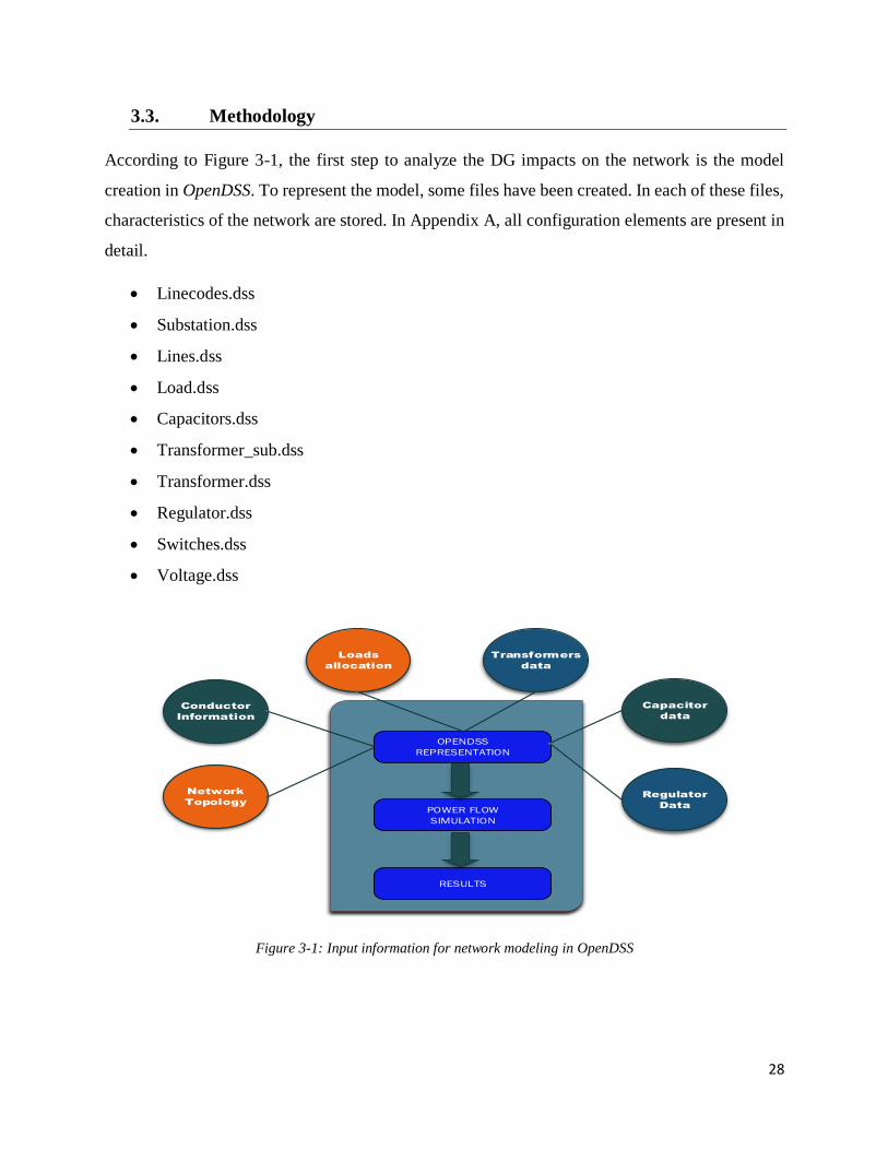
3.3. Methodology
According to Figure 3-1, the first step to analyze the DG impacts on the network is the model
creation in OpenDSS. To represent the model, some files have been created. In each of these files,
characteristics of the network are stored. In Appendix A, all configuration elements are present in
detail.
• Linecodes.dss
• Substation.dss
• Lines.dss
• Load.dss
• Capacitors.dss
• Transformer_sub.dss
• Transformer.dss
• Regulator.dss
• Switches.dss
• Voltage.dss
OPENDSS
REPRESENTATION
POWER FLOW
SIMULATION
Conductor
Information
Network
Topology
Loads
allocation
Transformers
data
Capacitor
data
Regulator
Data
RESULTS
Figure 3-1: Input information for network modeling in OpenDSS
29
3.3.1. Overview
To carry out an analysis of the impact of DG in the distribution network, it is necessary to make
comparisons with different DG penetration levels. The first step consists of analyzing a base case
without DG. After that, the procedure continues with the connection of certain amount of DG
penetration in a particular location of the network. Finally, the impacts of different penetration
levels are analyzed. Losses and voltages of the grid are particularly evaluated and compared with
the base case. An IEEE test feeder and a real network are analyzed. For each case study, two
methods to evaluate the impacts of DG are used; these methods are static and Quasi-Static Time
Series Analysis.
3.4. LOW VOLTAGE MODELS AND CREATING LOAD PROFILES
Distribution System
Electric power distribution is the portion of the power delivery infrastructure that takes the
electricity from the highly meshed, high-voltage transmission circuits and delivers it to customers
[30]. This distribution system typically starts with the substation that feeds one or more sub
transmission lines. In some cases, the distribution substation is fed directly from a high-voltage
transmission line in which case, most likely, there is not a sub-transmission system. Feeders are
radial with a rare exception [31].
30
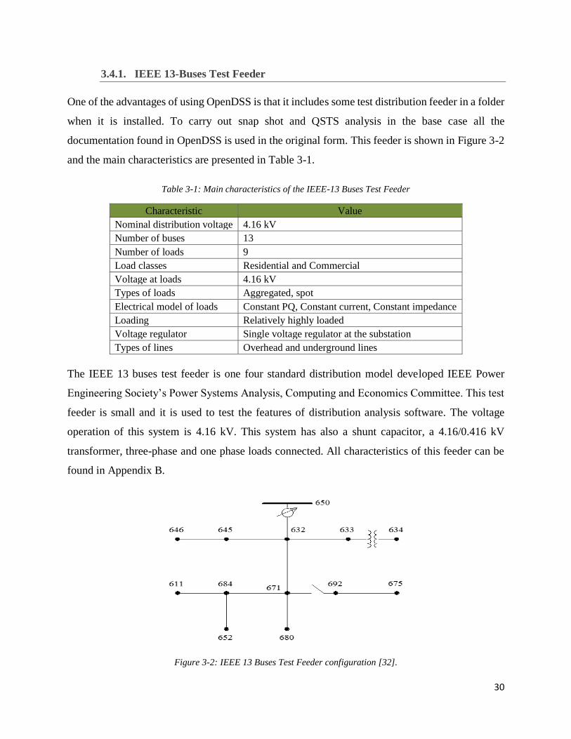
3.4.1. IEEE 13-Buses Test Feeder
One of the advantages of using OpenDSS is that it includes some test distribution feeder in a folder
when it is installed. To carry out snap shot and QSTS analysis in the base case all the
documentation found in OpenDSS is used in the original form. This feeder is shown in Figure 3-2
and the main characteristics are presented in Table 3-1.
Table 3-1: Main characteristics of the IEEE-13 Buses Test Feeder
Characteristic Value
Nominal distribution voltage 4.16 kV
Number of buses 13
Number of loads 9
Load classes Residential and Commercial
Voltage at loads 4.16 kV
Types of loads Aggregated, spot
Electrical model of loads Constant PQ, Constant current, Constant impedance
Loading Relatively highly loaded
Voltage regulator Single voltage regulator at the substation
Types of lines Overhead and underground lines
The IEEE 13 buses test feeder is one four standard distribution model developed IEEE Power
Engineering Society’s Power Systems Analysis, Computing and Economics Committee. This test
feeder is small and it is used to test the features of distribution analysis software. The voltage
operation of this system is 4.16 kV. This system has also a shunt capacitor, a 4.16/0.416 kV
transformer, three-phase and one phase loads connected. All characteristics of this feeder can be
found in Appendix B.
Figure 3-2: IEEE 13 Buses Test Feeder configuration [32].
31
3.4.2. Real Distribution Test System (CENTROSUR)
CENTROSUR low voltage system supplies energy to residential, commercial, small industrial
customers and public lighting. The level voltage is 120/240 for single phase systems, 120/208 V
and 127/220 V for three phases systems.
It is possible to analyze the behavior of the network in different operating scenarios through the
secondary circuit model. Transformers, lines, loads, and structures models are presented below.
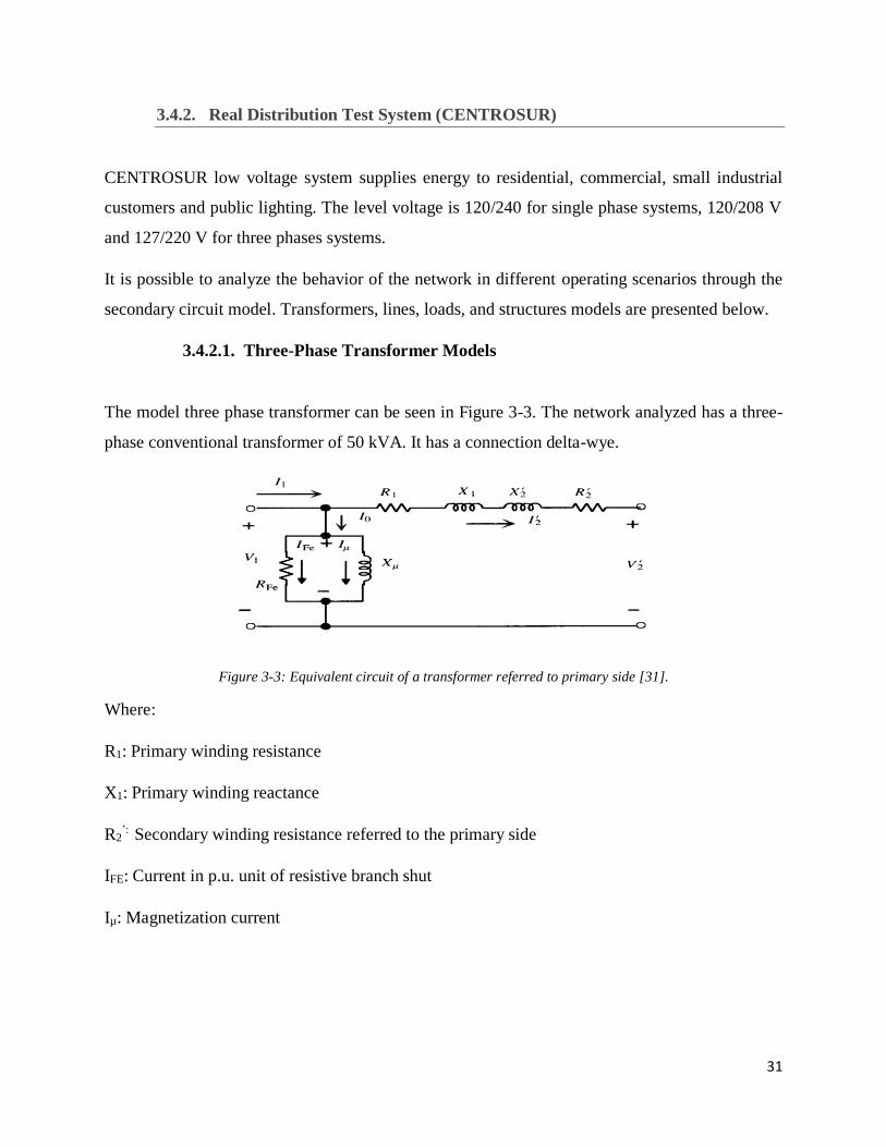
3.4.2.1. Three-Phase Transformer Models
The model three phase transformer can be seen in Figure 3-3. The network analyzed has a three-
phase conventional transformer of 50 kVA. It has a connection delta-wye.
Figure 3-3: Equivalent circuit of a transformer referred to primary side [31].
Where:
R1: Primary winding resistance
X1: Primary winding reactance
R2’: Secondary winding resistance referred to the primary side
IFE: Current in p.u. unit of resistive branch shut
Iµ: Magnetization current
32
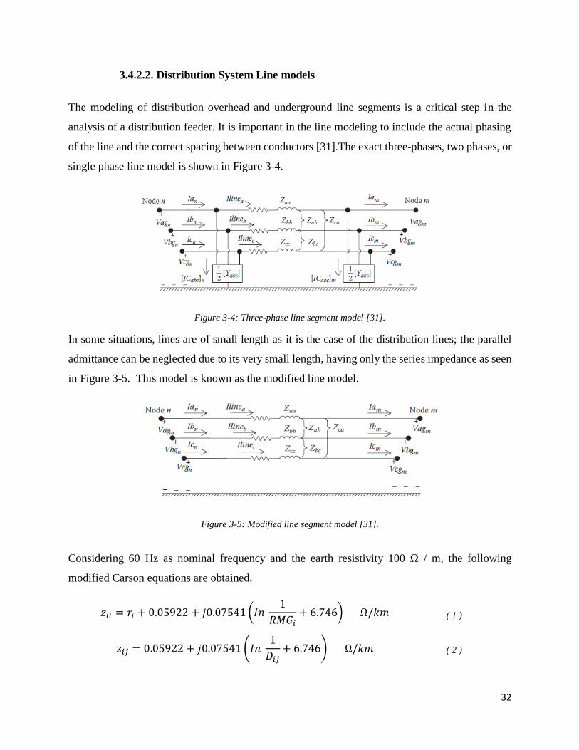
3.4.2.2. Distribution System Line models
The modeling of distribution overhead and underground line segments is a critical step in the
analysis of a distribution feeder. It is important in the line modeling to include the actual phasing
of the line and the correct spacing between conductors [31].The exact three-phases, two phases, or
single phase line model is shown in Figure 3-4.
Figure 3-4: Three-phase line segment model [31].
In some situations, lines are of small length as it is the case of the distribution lines; the parallel
admittance can be neglected due to its very small length, having only the series impedance as seen
in Figure 3-5. This model is known as the modified line model.
Figure 3-5: Modified line segment model [31].
Considering 60 Hz as nominal frequency and the earth resistivity 100 Ω / m, the following
modified Carson equations are obtained.
𝑧𝑖𝑖 = 𝑟𝑖 + 0.05922 + 𝑗0.07541 (𝐼𝑛 1
𝑅𝑀𝐺𝑖+ 6.746) Ω/𝑘𝑚 ( 1 )
𝑧𝑖𝑗 = 0.05922 + 𝑗0.07541 (𝐼𝑛 1
𝐷𝑖𝑗+ 6.746) Ω/𝑘𝑚 ( 2 )
33
Where:
𝑟𝑖: resistance wire Ω/km
𝑅𝑀𝐺𝑖: Geometric medium radius in meters
𝐷𝑖𝑗: Distance in meters between wire i and wire j
Through Eq.1 and Eq.2 it is possible to calculate the primitive impedance matrix of the line.
3.4.2.3. Load Models
Loads on the distribution system are specified by the consumed complex power. The specified
load will be the “maximum diversified demand”. This demand can be specified as kVA and power
factor, kW and power factor, or kW and kVAr.
Loads on distribution systems can be modeled as wye connected or delta connected. The load
models can be classified in static load model, ZIP models, and exponential models.
The exponential model of constant power was used in this work. For this model, active and
reactive power are presented by the following equations.
𝑃 = 𝑃0(𝑉
𝑉0)𝛼 ( 3 )
𝑄 = 𝑄0(𝑉
𝑉0)𝛽
( 4 )
Where 𝑃0 y 𝑄0 are active power and reactive power with nominal voltage.
V0 is the nominal voltage; α and β are exponential load parameters.
34
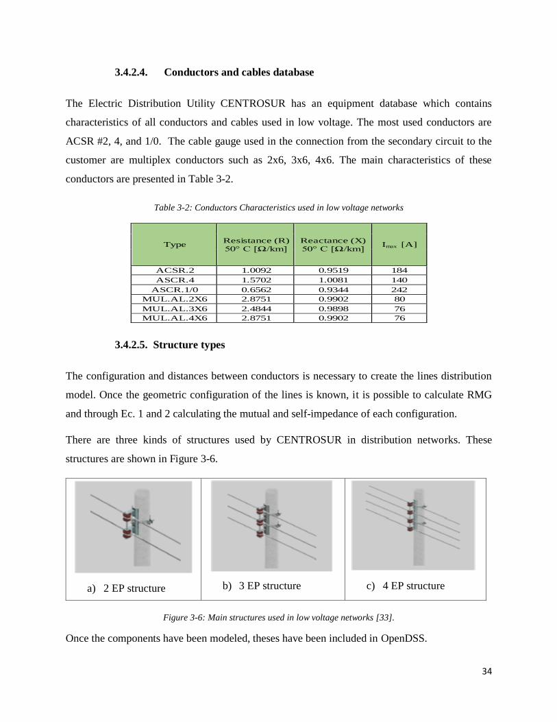
3.4.2.4. Conductors and cables database
The Electric Distribution Utility CENTROSUR has an equipment database which contains
characteristics of all conductors and cables used in low voltage. The most used conductors are
ACSR #2, 4, and 1/0. The cable gauge used in the connection from the secondary circuit to the
customer are multiplex conductors such as 2x6, 3x6, 4x6. The main characteristics of these
conductors are presented in Table 3-2.
Table 3-2: Conductors Characteristics used in low voltage networks
3.4.2.5. Structure types
The configuration and distances between conductors is necessary to create the lines distribution
model. Once the geometric configuration of the lines is known, it is possible to calculate RMG
and through Ec. 1 and 2 calculating the mutual and self-impedance of each configuration.
There are three kinds of structures used by CENTROSUR in distribution networks. These
structures are shown in Figure 3-6.
a) 2 EP structure
b) 3 EP structure
c) 4 EP structure
Figure 3-6: Main structures used in low voltage networks [33].
Once the components have been modeled, theses have been included in OpenDSS.
Type Resistance (R) 50° C [Ω/km]
Reactance (X) 50° C [Ω/km]
Imax [A]
ACSR.2 1.0092 0.9519 184
ASCR.4 1.5702 1.0081 140
ASCR.1/0 0.6562 0.9344 242
MUL.AL.2X6 2.8751 0.9902 80
MUL.AL.3X6 2.4844 0.9898 76
MUL.AL.4X6 2.8751 0.9902 76
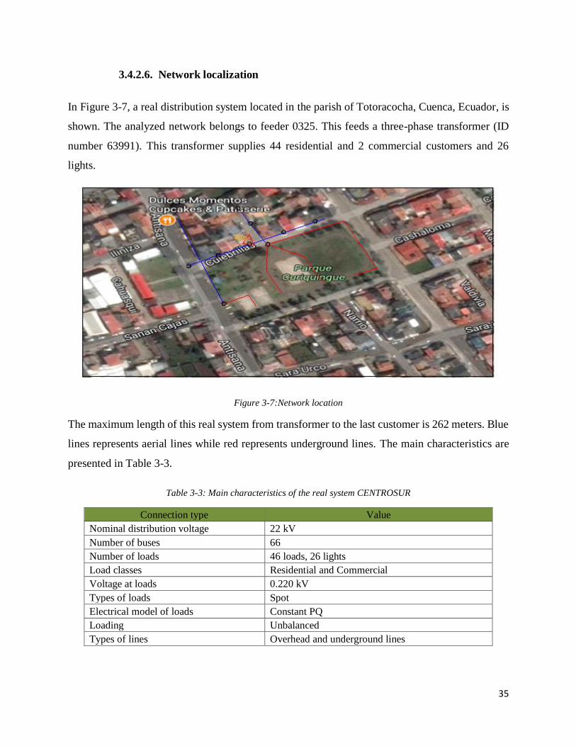
35
3.4.2.6. Network localization
In Figure 3-7, a real distribution system located in the parish of Totoracocha, Cuenca, Ecuador, is
shown. The analyzed network belongs to feeder 0325. This feeds a three-phase transformer (ID
number 63991). This transformer supplies 44 residential and 2 commercial customers and 26
lights.
Figure 3-7:Network location
The maximum length of this real system from transformer to the last customer is 262 meters. Blue
lines represents aerial lines while red represents underground lines. The main characteristics are
presented in Table 3-3.
Table 3-3: Main characteristics of the real system CENTROSUR
Connection type Value
Nominal distribution voltage 22 kV
Number of buses 66
Number of loads 46 loads, 26 lights
Load classes Residential and Commercial
Voltage at loads 0.220 kV
Types of loads Spot
Electrical model of loads Constant PQ
Loading Unbalanced
Types of lines Overhead and underground lines
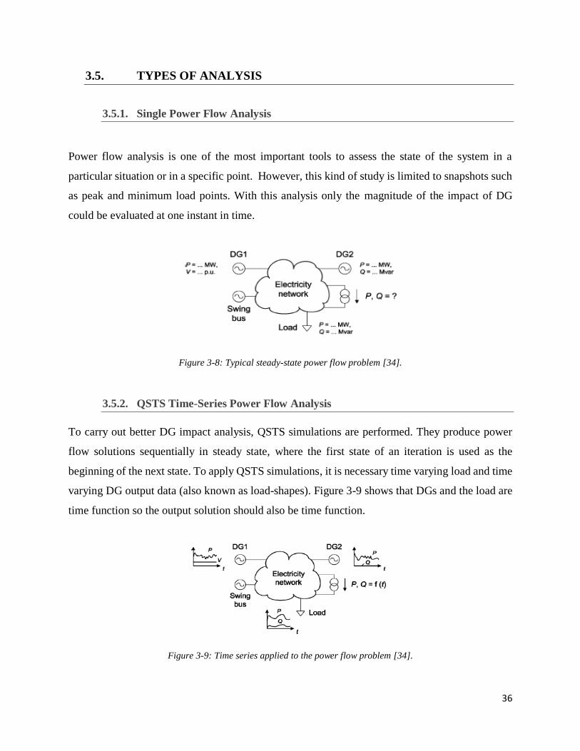
36
3.5. TYPES OF ANALYSIS
3.5.1. Single Power Flow Analysis
Power flow analysis is one of the most important tools to assess the state of the system in a
particular situation or in a specific point. However, this kind of study is limited to snapshots such
as peak and minimum load points. With this analysis only the magnitude of the impact of DG
could be evaluated at one instant in time.
Figure 3-8: Typical steady-state power flow problem [34].
3.5.2. QSTS Time-Series Power Flow Analysis
To carry out better DG impact analysis, QSTS simulations are performed. They produce power
flow solutions sequentially in steady state, where the first state of an iteration is used as the
beginning of the next state. To apply QSTS simulations, it is necessary time varying load and time
varying DG output data (also known as load-shapes). Figure 3-9 shows that DGs and the load are
time function so the output solution should also be time function.
Figure 3-9: Time series applied to the power flow problem [34].
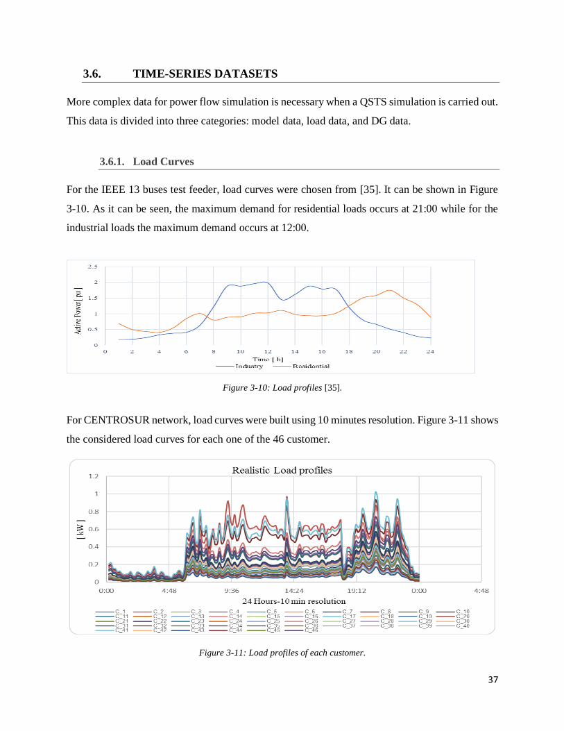
37
3.6. TIME-SERIES DATASETS
More complex data for power flow simulation is necessary when a QSTS simulation is carried out.
This data is divided into three categories: model data, load data, and DG data.
3.6.1. Load Curves
For the IEEE 13 buses test feeder, load curves were chosen from [35]. It can be shown in Figure
3-10. As it can be seen, the maximum demand for residential loads occurs at 21:00 while for the
industrial loads the maximum demand occurs at 12:00.
Figure 3-10: Load profiles [35].
For CENTROSUR network, load curves were built using 10 minutes resolution. Figure 3-11 shows
the considered load curves for each one of the 46 customer.
Figure 3-11: Load profiles of each customer.
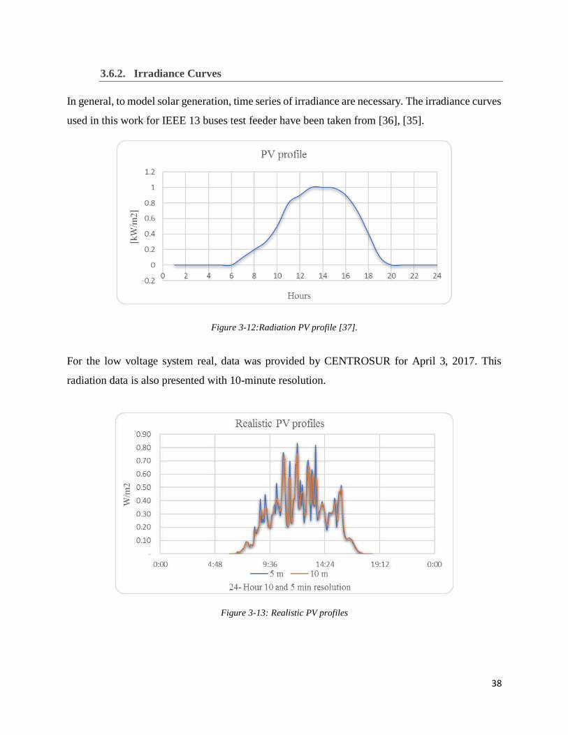
38
3.6.2. Irradiance Curves
In general, to model solar generation, time series of irradiance are necessary. The irradiance curves
used in this work for IEEE 13 buses test feeder have been taken from [36], [35].
Figure 3-12:Radiation PV profile [37].
For the low voltage system real, data was provided by CENTROSUR for April 3, 2017. This
radiation data is also presented with 10-minute resolution.
Figure 3-13: Realistic PV profiles
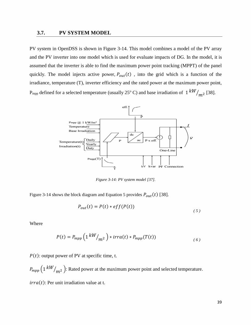
39
3.7. PV SYSTEM MODEL
PV system in OpenDSS is shown in Figure 3-14. This model combines a model of the PV array
and the PV inverter into one model which is used for evaluate impacts of DG. In the model, it is
assumed that the inverter is able to find the maximum power point tracking (MPPT) of the panel
quickly. The model injects active power, 𝑃𝑜𝑢𝑡(𝑡) , into the grid which is a function of the
irradiance, temperature (T), inverter efficiency and the rated power at the maximum power point,
Pmpp defined for a selected temperature (usually 25o C) and base irradiation of 1 𝑘𝑊𝑚2⁄ [38].
Figure 3-14: PV system model [37].
Figure 3-14 shows the block diagram and Equation 5 provides 𝑃𝑜𝑢𝑡(𝑡) [38].
𝑃𝑜𝑢𝑡(𝑡) = 𝑃(𝑡) ∗ 𝑒𝑓𝑓(𝑃(𝑡))
( 5 )
Where
𝑃(𝑡) = 𝑃𝑚𝑝𝑝 (1 𝑘𝑊𝑚2⁄ ) ∗ 𝑖𝑟𝑟𝑎(𝑡) ∗ 𝑃𝑚𝑝𝑝(𝑇(𝑡))
( 6 )
𝑃(𝑡): output power of PV at specific time, t.
𝑃𝑚𝑝𝑝 (1 𝑘𝑊𝑚2⁄ ): Rated power at the maximum power point and selected temperature.
𝑖𝑟𝑟𝑎(𝑡): Per unit irradiation value at t.
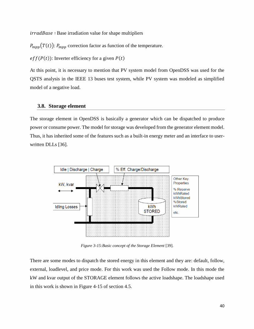
40
𝑖𝑟𝑟𝑎𝑑𝐵𝑎𝑠𝑒 ∶ Base irradiation value for shape multipliers
𝑃𝑚𝑝𝑝(𝑇(𝑡)): 𝑃𝑚𝑝𝑝 correction factor as function of the temperature.
𝑒𝑓𝑓(𝑃(𝑡)): Inverter efficiency for a given 𝑃(𝑡)
At this point, it is necessary to mention that PV system model from OpenDSS was used for the
QSTS analysis in the IEEE 13 buses test system, while PV system was modeled as simplified
model of a negative load.
3.8. Storage element
The storage element in OpenDSS is basically a generator which can be dispatched to produce
power or consume power. The model for storage was developed from the generator element model.
Thus, it has inherited some of the features such as a built-in energy meter and an interface to user-
written DLLs [36].
Figure 3-15:Basic concept of the Storage Element [39].
There are some modes to dispatch the stored energy in this element and they are: default, follow,
external, loadlevel, and price mode. For this work was used the Follow mode. In this mode the
kW and kvar output of the STORAGE element follows the active loadshape. The loadshape used
in this work is shown in Figure 4-15 of section 4.5.
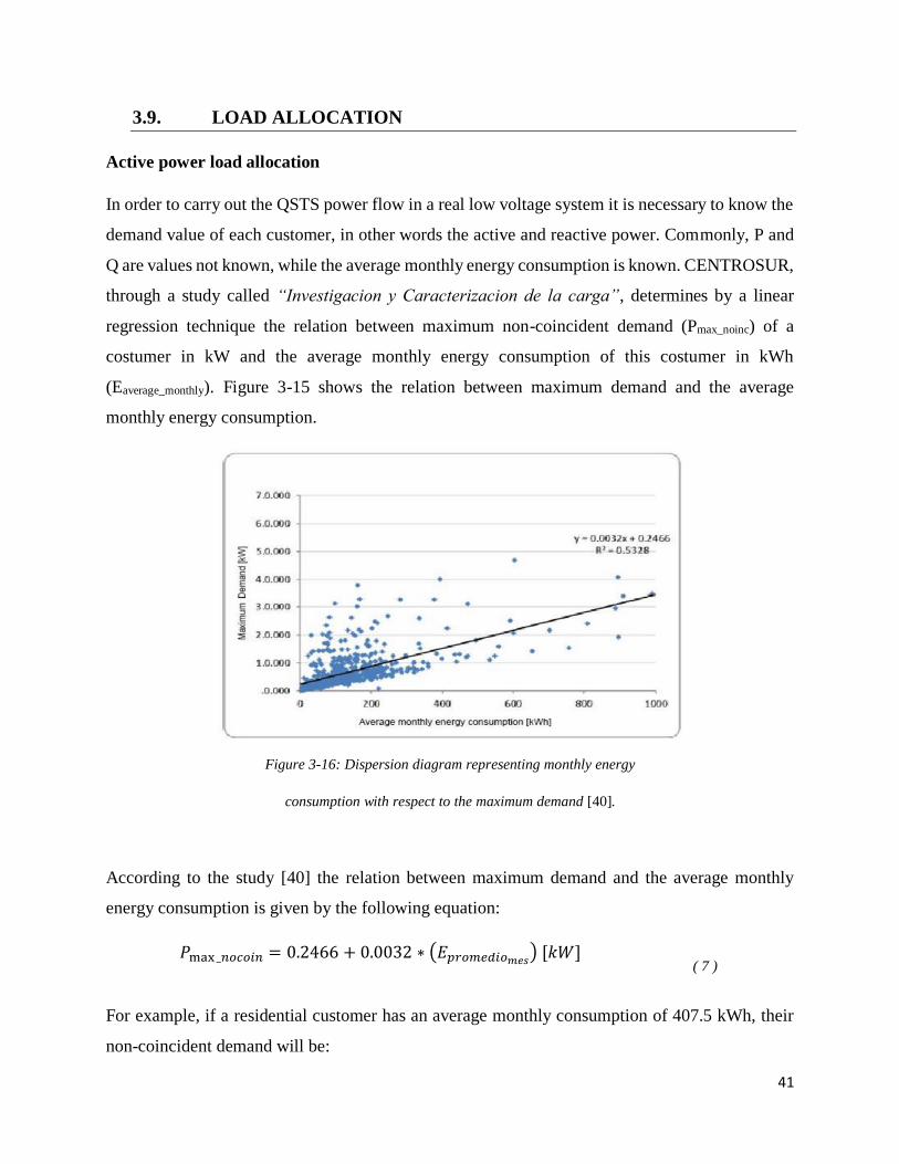
41
3.9. LOAD ALLOCATION
Active power load allocation
In order to carry out the QSTS power flow in a real low voltage system it is necessary to know the
demand value of each customer, in other words the active and reactive power. Commonly, P and
Q are values not known, while the average monthly energy consumption is known. CENTROSUR,
through a study called “Investigacion y Caracterizacion de la carga”, determines by a linear
regression technique the relation between maximum non-coincident demand (Pmax_noinc) of a
costumer in kW and the average monthly energy consumption of this costumer in kWh
(Eaverage_monthly). Figure 3-15 shows the relation between maximum demand and the average
monthly energy consumption.
Figure 3-16: Dispersion diagram representing monthly energy
consumption with respect to the maximum demand [40].
According to the study [40] the relation between maximum demand and the average monthly
energy consumption is given by the following equation:
𝑃max _𝑛𝑜𝑐𝑜𝑖𝑛 = 0.2466 + 0.0032 ∗ (𝐸𝑝𝑟𝑜𝑚𝑒𝑑𝑖𝑜𝑚𝑒𝑠) [𝑘𝑊]
( 7 )
For example, if a residential customer has an average monthly consumption of 407.5 kWh, their
non-coincident demand will be:
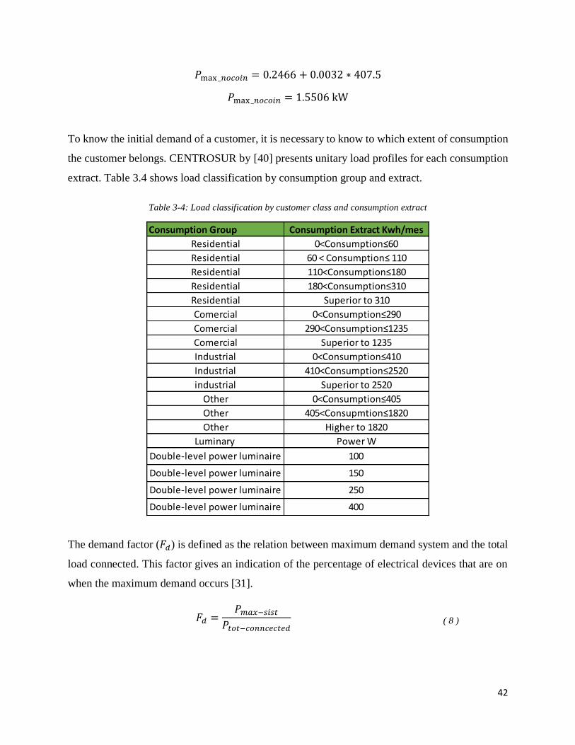
42
𝑃max _𝑛𝑜𝑐𝑜𝑖𝑛 = 0.2466 + 0.0032 ∗ 407.5
𝑃max _𝑛𝑜𝑐𝑜𝑖𝑛 = 1.5506 kW
To know the initial demand of a customer, it is necessary to know to which extent of consumption
the customer belongs. CENTROSUR by [40] presents unitary load profiles for each consumption
extract. Table 3.4 shows load classification by consumption group and extract.
Table 3-4: Load classification by customer class and consumption extract
The demand factor (𝐹𝑑) is defined as the relation between maximum demand system and the total
load connected. This factor gives an indication of the percentage of electrical devices that are on
when the maximum demand occurs [31].
𝐹𝑑 =𝑃𝑚𝑎𝑥−𝑠𝑖𝑠𝑡
𝑃𝑡𝑜𝑡−𝑐𝑜𝑛𝑛𝑐𝑒𝑐𝑡𝑒𝑑
( 8 )
Consumption Group Consumption Extract Kwh/mes
Residential 0<Consumption≤60
Residential 60 < Consumption≤ 110
Residential 110<Consumption≤180
Residential 180<Consumption≤310
Residential Superior to 310
Comercial 0<Consumption≤290
Comercial 290<Consumption≤1235
Comercial Superior to 1235
Industrial 0<Consumption≤410
Industrial 410<Consumption≤2520
industrial Superior to 2520
Other 0<Consumption≤405
Other 405<Consupmtion≤1820
Other Higher to 1820
Luminary Power W
Double-level power luminaire 100
Double-level power luminaire 150
Double-level power luminaire 250
Double-level power luminaire 400
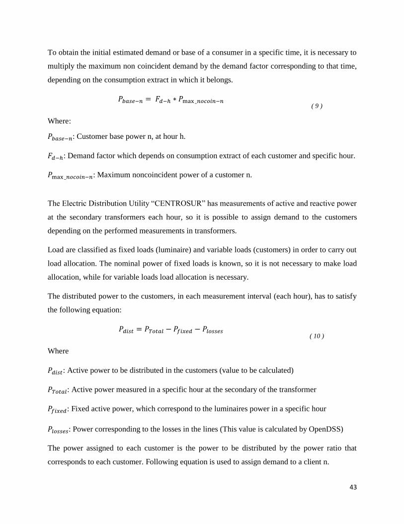
43
To obtain the initial estimated demand or base of a consumer in a specific time, it is necessary to
multiply the maximum non coincident demand by the demand factor corresponding to that time,
depending on the consumption extract in which it belongs.
𝑃𝑏𝑎𝑠𝑒−𝑛 = 𝐹𝑑−ℎ ∗ 𝑃max _𝑛𝑜𝑐𝑜𝑖𝑛−𝑛 ( 9 )
Where:
𝑃𝑏𝑎𝑠𝑒−𝑛: Customer base power n, at hour h.
𝐹𝑑−ℎ: Demand factor which depends on consumption extract of each customer and specific hour.
𝑃max _𝑛𝑜𝑐𝑜𝑖𝑛−𝑛: Maximum noncoincident power of a customer n.
The Electric Distribution Utility “CENTROSUR” has measurements of active and reactive power
at the secondary transformers each hour, so it is possible to assign demand to the customers
depending on the performed measurements in transformers.
Load are classified as fixed loads (luminaire) and variable loads (customers) in order to carry out
load allocation. The nominal power of fixed loads is known, so it is not necessary to make load
allocation, while for variable loads load allocation is necessary.
The distributed power to the customers, in each measurement interval (each hour), has to satisfy
the following equation:
𝑃𝑑𝑖𝑠𝑡 = 𝑃𝑇𝑜𝑡𝑎𝑙 − 𝑃𝑓𝑖𝑥𝑒𝑑 − 𝑃𝑙𝑜𝑠𝑠𝑒𝑠 ( 10 )
Where
𝑃𝑑𝑖𝑠𝑡: Active power to be distributed in the customers (value to be calculated)
𝑃𝑇𝑜𝑡𝑎𝑙: Active power measured in a specific hour at the secondary of the transformer
𝑃𝑓𝑖𝑥𝑒𝑑: Fixed active power, which correspond to the luminaires power in a specific hour
𝑃𝑙𝑜𝑠𝑠𝑒𝑠: Power corresponding to the losses in the lines (This value is calculated by OpenDSS)
The power assigned to each customer is the power to be distributed by the power ratio that
corresponds to each customer. Following equation is used to assign demand to a client n.
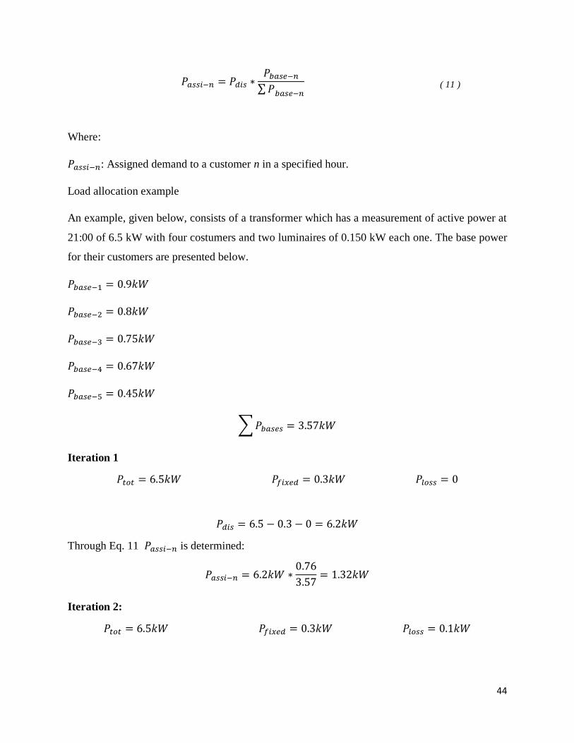
44
𝑃𝑎𝑠𝑠𝑖−𝑛 = 𝑃𝑑𝑖𝑠 ∗𝑃𝑏𝑎𝑠𝑒−𝑛
∑ 𝑃𝑏𝑎𝑠𝑒−𝑛
( 11 )
Where:
𝑃𝑎𝑠𝑠𝑖−𝑛: Assigned demand to a customer n in a specified hour.
Load allocation example
An example, given below, consists of a transformer which has a measurement of active power at
21:00 of 6.5 kW with four costumers and two luminaires of 0.150 kW each one. The base power
for their customers are presented below.
𝑃𝑏𝑎𝑠𝑒−1 = 0.9𝑘𝑊
𝑃𝑏𝑎𝑠𝑒−2 = 0.8𝑘𝑊
𝑃𝑏𝑎𝑠𝑒−3 = 0.75𝑘𝑊
𝑃𝑏𝑎𝑠𝑒−4 = 0.67𝑘𝑊
𝑃𝑏𝑎𝑠𝑒−5 = 0.45𝑘𝑊
∑ 𝑃𝑏𝑎𝑠𝑒𝑠 = 3.57𝑘𝑊
Iteration 1
𝑃𝑡𝑜𝑡 = 6.5𝑘𝑊 𝑃𝑓𝑖𝑥𝑒𝑑 = 0.3𝑘𝑊 𝑃𝑙𝑜𝑠𝑠 = 0
𝑃𝑑𝑖𝑠 = 6.5 − 0.3 − 0 = 6.2𝑘𝑊
Through Eq. 11 𝑃𝑎𝑠𝑠𝑖−𝑛 is determined:
𝑃𝑎𝑠𝑠𝑖−𝑛 = 6.2𝑘𝑊 ∗0.76
3.57= 1.32𝑘𝑊
Iteration 2:
𝑃𝑡𝑜𝑡 = 6.5𝑘𝑊 𝑃𝑓𝑖𝑥𝑒𝑑 = 0.3𝑘𝑊 𝑃𝑙𝑜𝑠𝑠 = 0.1𝑘𝑊
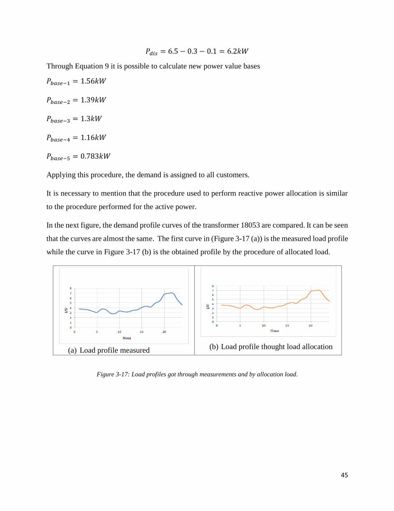
45
𝑃𝑑𝑖𝑠 = 6.5 − 0.3 − 0.1 = 6.2𝑘𝑊
Through Equation 9 it is possible to calculate new power value bases
𝑃𝑏𝑎𝑠𝑒−1 = 1.56𝑘𝑊
𝑃𝑏𝑎𝑠𝑒−2 = 1.39𝑘𝑊
𝑃𝑏𝑎𝑠𝑒−3 = 1.3𝑘𝑊
𝑃𝑏𝑎𝑠𝑒−4 = 1.16𝑘𝑊
𝑃𝑏𝑎𝑠𝑒−5 = 0.783𝑘𝑊
Applying this procedure, the demand is assigned to all customers.
It is necessary to mention that the procedure used to perform reactive power allocation is similar
to the procedure performed for the active power.
In the next figure, the demand profile curves of the transformer 18053 are compared. It can be seen
that the curves are almost the same. The first curve in (Figure 3-17 (a)) is the measured load profile
while the curve in Figure 3-17 (b) is the obtained profile by the procedure of allocated load.
(a) Load profile measured
(b) Load profile thought load allocation
Figure 3-17: Load profiles got through measurements and by allocation load.

46
47
4. SIMULATIONS AND TEST RESULTS
4.2. IEEE 13 BUSES SNAPSHOT SIMULATION
Five different scenarios have been defined in order to evaluate technical features such as losses
and voltages profiles after the integration of DG in this network. In these scenarios, it was
considered different penetration scenarios of DG. Each scenario was considered according to the
penetration percentage which, is defined by the following equation.
%𝑃𝑒𝑛𝑒𝑡𝑟𝑎𝑡𝑖𝑜𝑛 =𝑃𝑒𝑎𝑘 𝑃𝑜𝑤𝑒𝑟 𝐷𝐺
𝑃𝑒𝑎𝑘 𝐿𝑜𝑎𝑑 [𝑘𝑤] (12)
• The first scenario (Scenario base) is the scenario that does not include DG.
• Scenario 2 represents the effect of including a 10 % of DG penetration. In this scenario,
DG was distributed proportionally to the load in all buses by an OpenDSS command.
• In scenario 3, 10% of DG penetration is distributed at 675 and 680 buses.
• In scenario 4, 20% of the total load DG penetration is distributed at 675 and 680 buses.
• Finally, scenario 5, 50% of the total load DG penetration is added at the same nodes
considered previously.
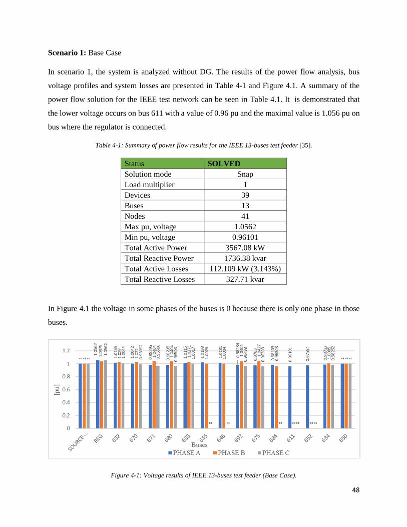
48
Scenario 1: Base Case
In scenario 1, the system is analyzed without DG. The results of the power flow analysis, bus
voltage profiles and system losses are presented in Table 4-1 and Figure 4.1. A summary of the
power flow solution for the IEEE test network can be seen in Table 4.1. It is demonstrated that
the lower voltage occurs on bus 611 with a value of 0.96 pu and the maximal value is 1.056 pu on
bus where the regulator is connected.
Table 4-1: Summary of power flow results for the IEEE 13-buses test feeder [35].
Status SOLVED
Solution mode Snap
Load multiplier 1
Devices 39
Buses 13
Nodes 41
Max pu, voltage 1.0562
Min pu, voltage 0.96101
Total Active Power 3567.08 kW
Total Reactive Power 1736.38 kvar
Total Active Losses 112.109 kW (3.143%)
Total Reactive Losses 327.71 kvar
In Figure 4.1 the voltage in some phases of the buses is 0 because there is only one phase in those
buses.
Figure 4-1: Voltage results of IEEE 13-buses test feeder (Base Case).
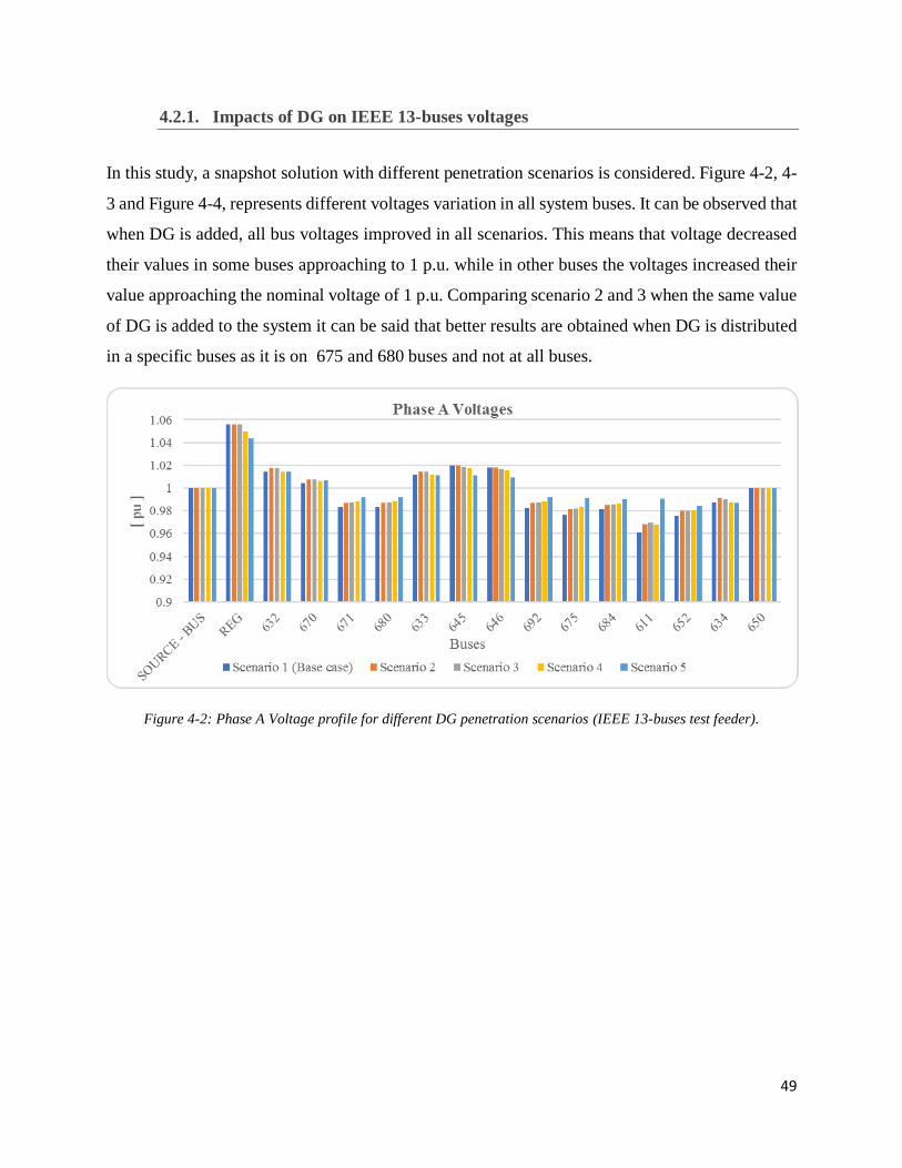
49
4.2.1. Impacts of DG on IEEE 13-buses voltages
In this study, a snapshot solution with different penetration scenarios is considered. Figure 4-2, 4-
3 and Figure 4-4, represents different voltages variation in all system buses. It can be observed that
when DG is added, all bus voltages improved in all scenarios. This means that voltage decreased
their values in some buses approaching to 1 p.u. while in other buses the voltages increased their
value approaching the nominal voltage of 1 p.u. Comparing scenario 2 and 3 when the same value
of DG is added to the system it can be said that better results are obtained when DG is distributed
in a specific buses as it is on 675 and 680 buses and not at all buses.
Figure 4-2: Phase A Voltage profile for different DG penetration scenarios (IEEE 13-buses test feeder).
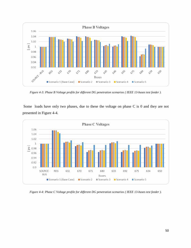
50
Figure 4-3: Phase B Voltage profile for different DG penetration scenarios ( IEEE 13-buses test feeder ).
Some loads have only two phases, due to these the voltage on phase C is 0 and they are not
presented in Figure 4-4.
Figure 4-4: Phase C Voltage profile for different DG penetration scenarios ( IEEE 13-buses test feeder ).
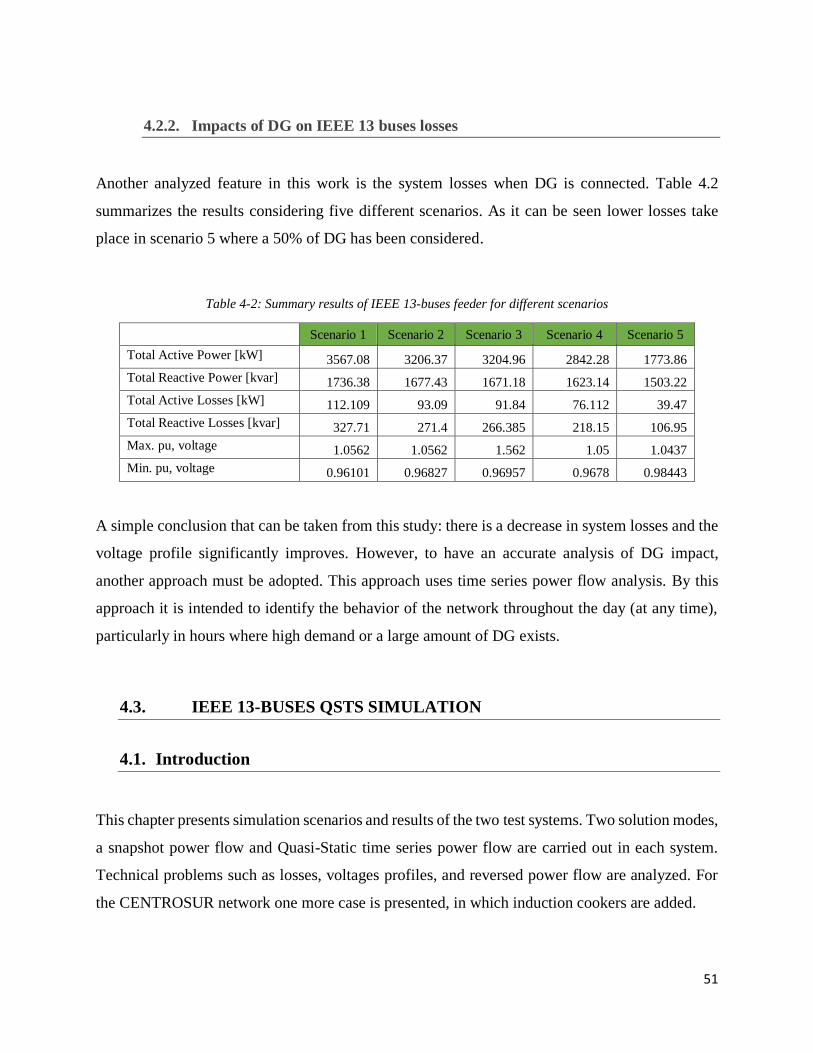
51
4.2.2. Impacts of DG on IEEE 13 buses losses
Another analyzed feature in this work is the system losses when DG is connected. Table 4.2
summarizes the results considering five different scenarios. As it can be seen lower losses take
place in scenario 5 where a 50% of DG has been considered.
Table 4-2: Summary results of IEEE 13-buses feeder for different scenarios
Scenario 1 Scenario 2 Scenario 3 Scenario 4 Scenario 5
Total Active Power [kW] 3567.08 3206.37 3204.96 2842.28 1773.86
Total Reactive Power [kvar] 1736.38 1677.43 1671.18 1623.14 1503.22
Total Active Losses [kW] 112.109 93.09 91.84 76.112 39.47
Total Reactive Losses [kvar] 327.71 271.4 266.385 218.15 106.95
Max. pu, voltage 1.0562 1.0562 1.562 1.05 1.0437
Min. pu, voltage 0.96101 0.96827 0.96957 0.9678 0.98443
A simple conclusion that can be taken from this study: there is a decrease in system losses and the
voltage profile significantly improves. However, to have an accurate analysis of DG impact,
another approach must be adopted. This approach uses time series power flow analysis. By this
approach it is intended to identify the behavior of the network throughout the day (at any time),
particularly in hours where high demand or a large amount of DG exists.
4.3. IEEE 13-BUSES QSTS SIMULATION
4.1. Introduction
This chapter presents simulation scenarios and results of the two test systems. Two solution modes,
a snapshot power flow and Quasi-Static time series power flow are carried out in each system.
Technical problems such as losses, voltages profiles, and reversed power flow are analyzed. For
the CENTROSUR network one more case is presented, in which induction cookers are added.
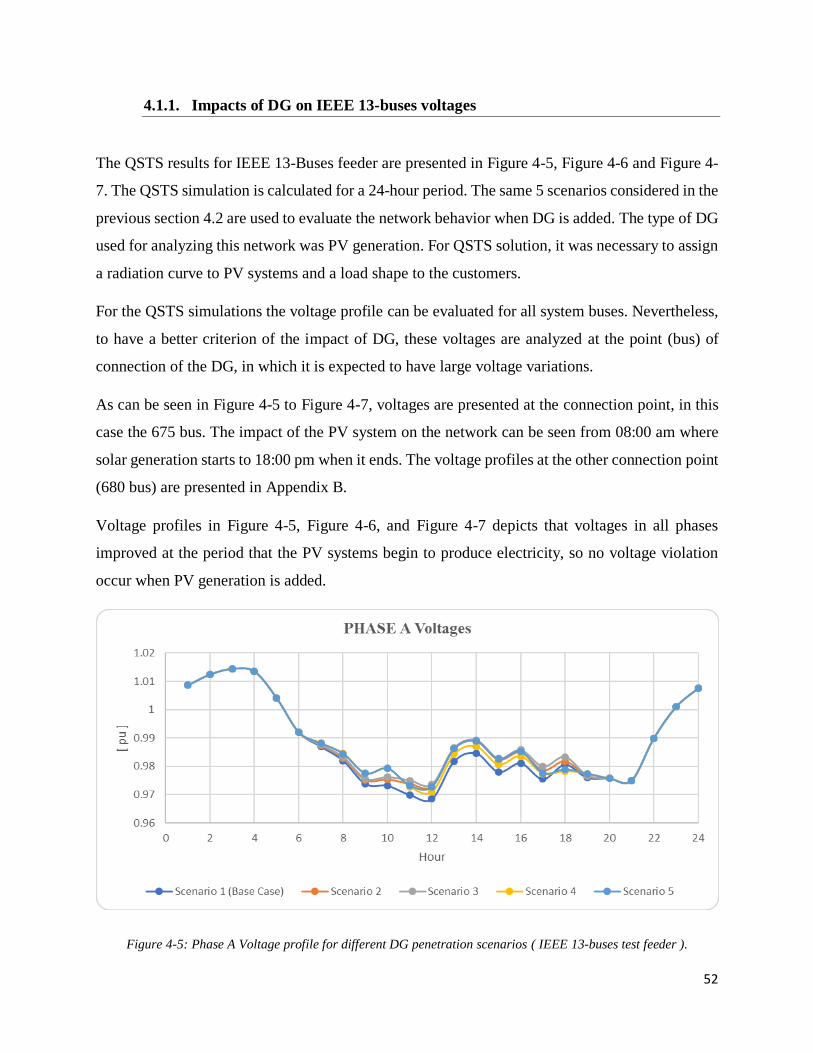
52
4.1.1. Impacts of DG on IEEE 13-buses voltages
The QSTS results for IEEE 13-Buses feeder are presented in Figure 4-5, Figure 4-6 and Figure 4-
7. The QSTS simulation is calculated for a 24-hour period. The same 5 scenarios considered in the
previous section 4.2 are used to evaluate the network behavior when DG is added. The type of DG
used for analyzing this network was PV generation. For QSTS solution, it was necessary to assign
a radiation curve to PV systems and a load shape to the customers.
For the QSTS simulations the voltage profile can be evaluated for all system buses. Nevertheless,
to have a better criterion of the impact of DG, these voltages are analyzed at the point (bus) of
connection of the DG, in which it is expected to have large voltage variations.
As can be seen in Figure 4-5 to Figure 4-7, voltages are presented at the connection point, in this
case the 675 bus. The impact of the PV system on the network can be seen from 08:00 am where
solar generation starts to 18:00 pm when it ends. The voltage profiles at the other connection point
(680 bus) are presented in Appendix B.
Voltage profiles in Figure 4-5, Figure 4-6, and Figure 4-7 depicts that voltages in all phases
improved at the period that the PV systems begin to produce electricity, so no voltage violation
occur when PV generation is added.
Figure 4-5: Phase A Voltage profile for different DG penetration scenarios ( IEEE 13-buses test feeder ).
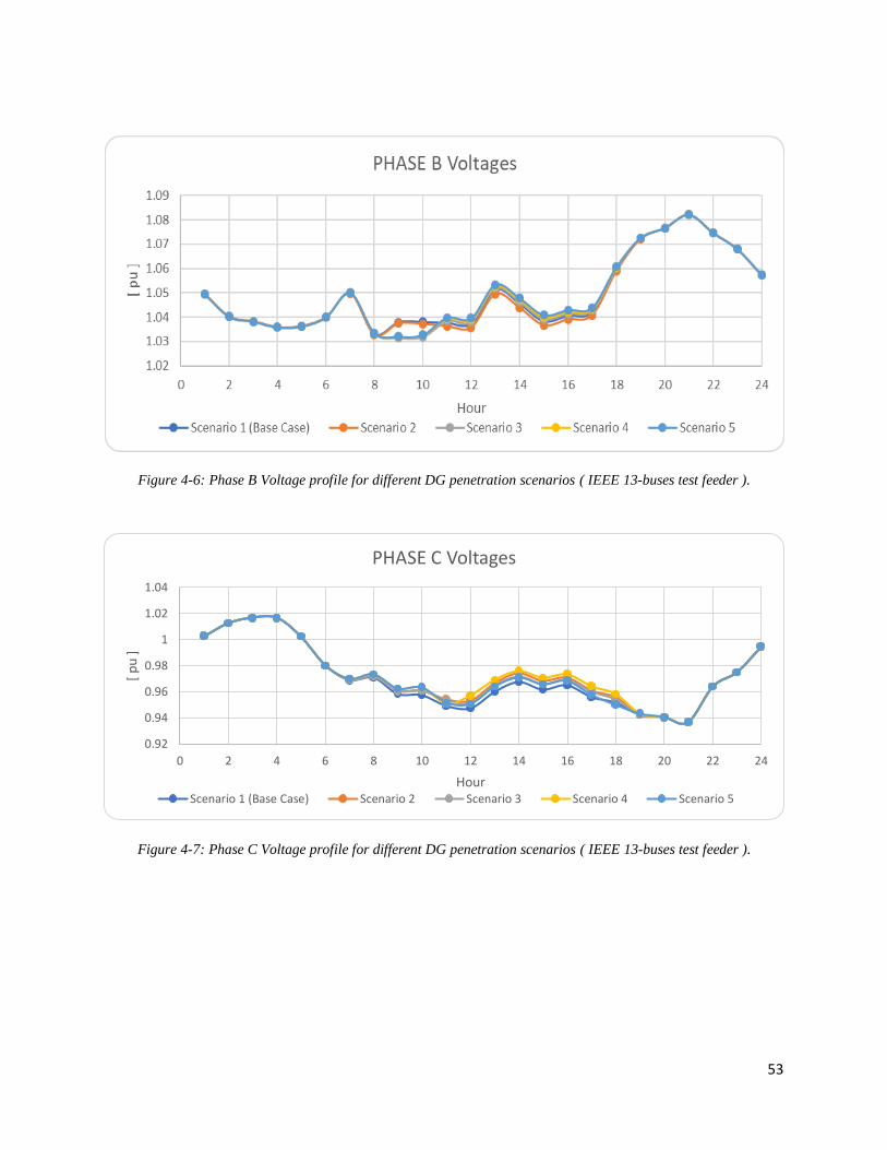
53
Figure 4-6: Phase B Voltage profile for different DG penetration scenarios ( IEEE 13-buses test feeder ).
Figure 4-7: Phase C Voltage profile for different DG penetration scenarios ( IEEE 13-buses test feeder ).
0.92
0.94
0.96
0.98
1
1.02
1.04
0 2 4 6 8 10 12 14 16 18 20 22 24
[ p
u ]
Hour
PHASE C Voltages
Scenario 1 (Base Case) Scenario 2 Scenario 3 Scenario 4 Scenario 5
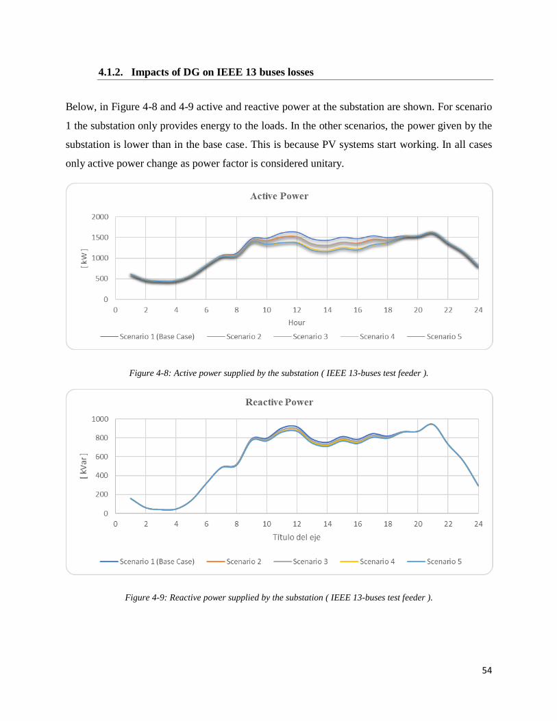
54
4.1.2. Impacts of DG on IEEE 13 buses losses
Below, in Figure 4-8 and 4-9 active and reactive power at the substation are shown. For scenario
1 the substation only provides energy to the loads. In the other scenarios, the power given by the
substation is lower than in the base case. This is because PV systems start working. In all cases
only active power change as power factor is considered unitary.
Figure 4-8: Active power supplied by the substation ( IEEE 13-buses test feeder ).
Figure 4-9: Reactive power supplied by the substation ( IEEE 13-buses test feeder ).
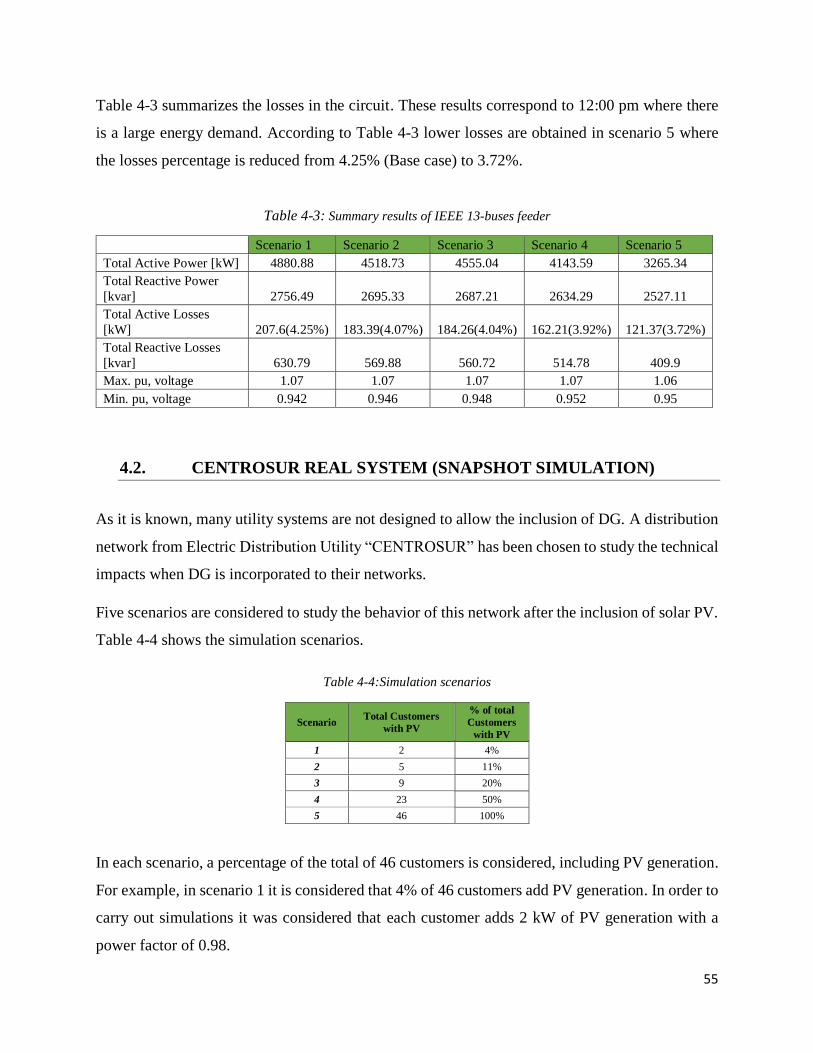
55
Table 4-3 summarizes the losses in the circuit. These results correspond to 12:00 pm where there
is a large energy demand. According to Table 4-3 lower losses are obtained in scenario 5 where
the losses percentage is reduced from 4.25% (Base case) to 3.72%.
Table 4-3: Summary results of IEEE 13-buses feeder
Scenario 1 Scenario 2 Scenario 3 Scenario 4 Scenario 5
Total Active Power [kW] 4880.88 4518.73 4555.04 4143.59 3265.34
Total Reactive Power
[kvar] 2756.49 2695.33 2687.21 2634.29 2527.11
Total Active Losses
[kW] 207.6(4.25%) 183.39(4.07%) 184.26(4.04%) 162.21(3.92%) 121.37(3.72%)
Total Reactive Losses
[kvar] 630.79 569.88 560.72 514.78 409.9
Max. pu, voltage 1.07 1.07 1.07 1.07 1.06
Min. pu, voltage 0.942 0.946 0.948 0.952 0.95
4.2. CENTROSUR REAL SYSTEM (SNAPSHOT SIMULATION)
As it is known, many utility systems are not designed to allow the inclusion of DG. A distribution
network from Electric Distribution Utility “CENTROSUR” has been chosen to study the technical
impacts when DG is incorporated to their networks.
Five scenarios are considered to study the behavior of this network after the inclusion of solar PV.
Table 4-4 shows the simulation scenarios.
Table 4-4:Simulation scenarios
Scenario Total Customers
with PV
% of total
Customers
with PV
1 2 4%
2 5 11%
3 9 20%
4 23 50%
5 46 100%
In each scenario, a percentage of the total of 46 customers is considered, including PV generation.
For example, in scenario 1 it is considered that 4% of 46 customers add PV generation. In order to
carry out simulations it was considered that each customer adds 2 kW of PV generation with a
power factor of 0.98.
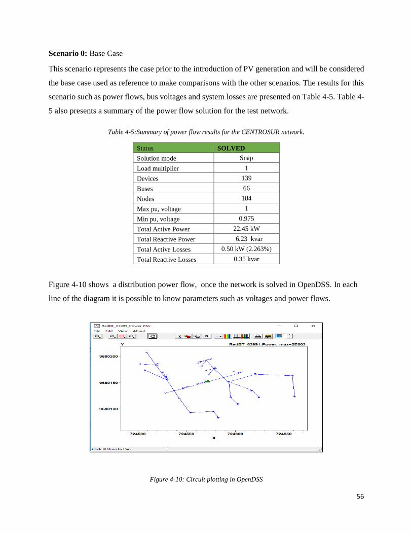
56
Scenario 0: Base Case
This scenario represents the case prior to the introduction of PV generation and will be considered
the base case used as reference to make comparisons with the other scenarios. The results for this
scenario such as power flows, bus voltages and system losses are presented on Table 4-5. Table 4-
5 also presents a summary of the power flow solution for the test network.
Table 4-5:Summary of power flow results for the CENTROSUR network.
Status SOLVED
Solution mode Snap
Load multiplier 1
Devices 139
Buses 66
Nodes 184
Max pu, voltage 1
Min pu, voltage 0.975
Total Active Power 22.45 kW
Total Reactive Power 6.23 kvar
Total Active Losses 0.50 kW (2.263%)
Total Reactive Losses 0.35 kvar
Figure 4-10 shows a distribution power flow, once the network is solved in OpenDSS. In each
line of the diagram it is possible to know parameters such as voltages and power flows.
Figure 4-10: Circuit plotting in OpenDSS
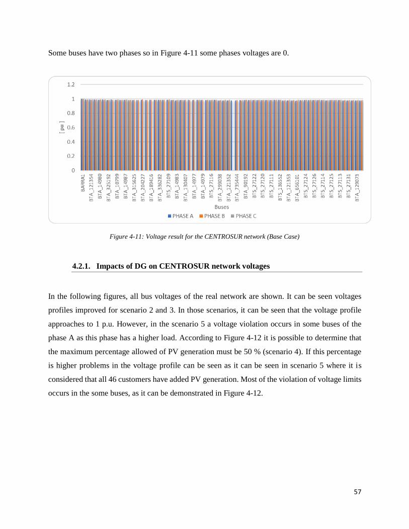
57
Some buses have two phases so in Figure 4-11 some phases voltages are 0.
Figure 4-11: Voltage result for the CENTROSUR network (Base Case)
4.2.1. Impacts of DG on CENTROSUR network voltages
In the following figures, all bus voltages of the real network are shown. It can be seen voltages
profiles improved for scenario 2 and 3. In those scenarios, it can be seen that the voltage profile
approaches to 1 p.u. However, in the scenario 5 a voltage violation occurs in some buses of the
phase A as this phase has a higher load. According to Figure 4-12 it is possible to determine that
the maximum percentage allowed of PV generation must be 50 % (scenario 4). If this percentage
is higher problems in the voltage profile can be seen as it can be seen in scenario 5 where it is
considered that all 46 customers have added PV generation. Most of the violation of voltage limits
occurs in the some buses, as it can be demonstrated in Figure 4-12.
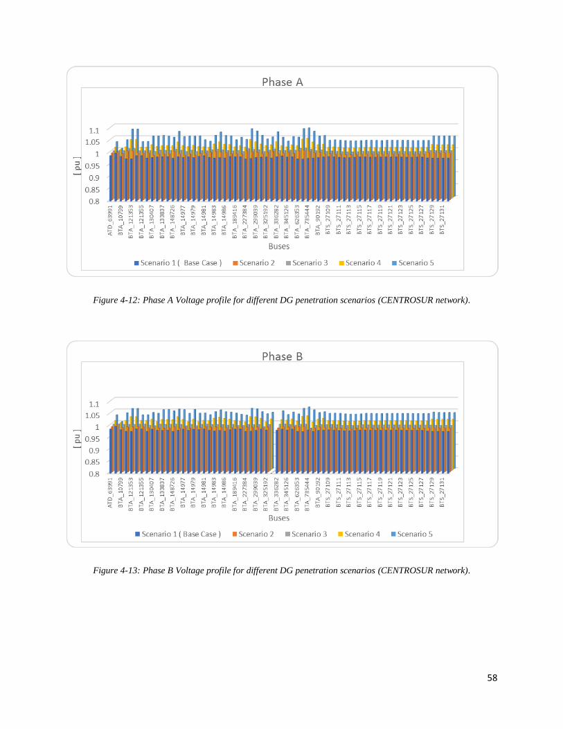
58
Figure 4-12: Phase A Voltage profile for different DG penetration scenarios (CENTROSUR network).
Figure 4-13: Phase B Voltage profile for different DG penetration scenarios (CENTROSUR network).
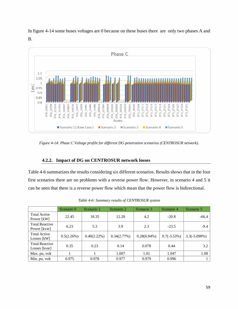
59
In figure 4-14 some buses voltages are 0 because on these buses there are only two phases A and
B.
Figure 4-14: Phase C Voltage profile for different DG penetration scenarios (CENTROSUR network).
4.2.2. Impact of DG on CENTROSUR network losses
Table 4-6 summarizes the results considering six different scenarios. Results shows that in the four
first scenarios there are no problems with a reverse power flow. However, in scenario 4 and 5 it
can be seen that there is a reverse power flow which mean that the power flow is bidirectional.
Table 4-6: Summary results of CENTROSUR system
Scenario 0 Scenario 1 Scenario 2 Scenario 3 Scenario 4 Scenario 5
Total Active
Power [kW] 22.45 18.35 12.28 4.2 -20.8 -66.4
Total Reactive
Power [kvar] 6.23 5.3 3.9 2.3 -23.5 -9.4
Total Active
Losses [kW] 0.5(2.26%) 0.40(2.22%) 0.34(2.77%) 0.28(6.84%) 0.7(-3.53%) 3.3(-5.098%)
Total Reactive
Losses [kvar] 0.35 0.23 0.14 0.078 0.44 3.2
Max. pu, volt 1 1 1.007 1.01 1.047 1.08
Min. pu, volt 0.975 0.978 0.977 0.979 0.996 1

60
4.3. CENTROSUR NETWORK QSTS SOLUTION
For this solution mode, three case studies have been selected. For each case, the same scenarios
considered for mode snapshot in Table 4-4 are taken. In figure 4-15 load shapes of PV generation,
storage systems, induction cookers and transformer demands are shown.
Figure 4-15:Unitary load profiles
4.3.1. CASE 1: PV
4.3.1.1. Impacts of DG on CENTROSUR network losses
This case considers the PV generation inclusion for each customer according to the scenarios
shown in Table 4-4. The QSTS power flow results for this case are presented below in Figure 4-
16.
Once carried out simulations, it can be shown that the maximum demand occurs at 20:00 pm for
scenario 1, where PV generation is not included. As the customers start to add PV generation
simulated in the different scenarios, it will be required a lower energy demand from the grid.
Simulation results shows that there are no problems with the first three scenarios. On the other
hand, results show a reversal of active power flow from customers back to the substation with 50%
(scenario 5) accumulated PV connection during the day. From Figure 4-15 it can be seen that PV
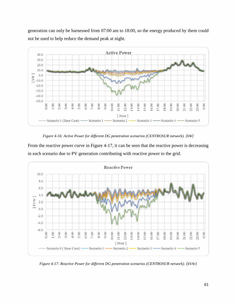
61
generation can only be harnessed from 07:00 am to 18:00, so the energy produced by them could
not be used to help reduce the demand peak at night.
Figure 4-16: Active Power for different DG penetration scenarios (CENTROSUR network). [kW]
From the reactive power curve in Figure 4-17, it can be seen that the reactive power is decreasing
in each scenario due to PV generation contributing with reactive power to the grid.
Figure 4-17: Reactive Power for different DG penetration scenarios (CENTROSUR network). [kVAr]
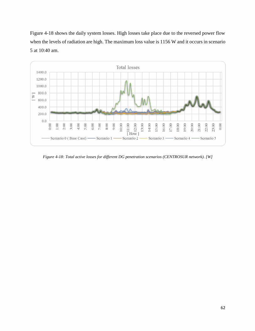
62
Figure 4-18 shows the daily system losses. High losses take place due to the reversed power flow
when the levels of radiation are high. The maximum loss value is 1156 W and it occurs in scenario
5 at 10:40 am.
Figure 4-18: Total active losses for different DG penetration scenarios (CENTROSUR network). [W]
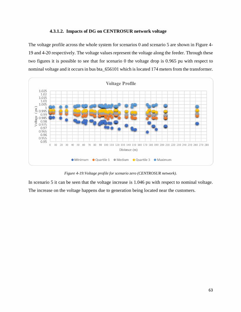
63
4.3.1.2. Impacts of DG on CENTROSUR network voltage
The voltage profile across the whole system for scenarios 0 and scenario 5 are shown in Figure 4-
19 and 4-20 respectively. The voltage values represent the voltage along the feeder. Through these
two figures it is possible to see that for scenario 0 the voltage drop is 0.965 pu with respect to
nominal voltage and it occurs in bus bta_656101 which is located 174 meters from the transformer.
Figure 4-19:Voltage profile for scenario zero (CENTROSUR network).
In scenario 5 it can be seen that the voltage increase is 1.046 pu with respect to nominal voltage.
The increase on the voltage happens due to generation being located near the customers.
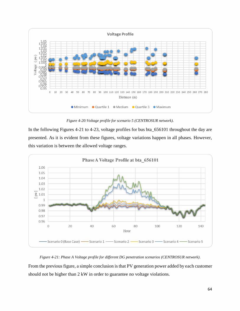
64
Figure 4-20:Voltage profile for scenario 5 (CENTROSUR network).
In the following Figures 4-21 to 4-23, voltage profiles for bus bta_656101 throughout the day are
presented. As it is evident from these figures, voltage variations happen in all phases. However,
this variation is between the allowed voltage ranges.
Figure 4-21: Phase A Voltage profile for different DG penetration scenarios (CENTROSUR network).
From the previous figure, a simple conclusion is that PV generation power added by each customer
should not be higher than 2 kW in order to guarantee no voltage violations.
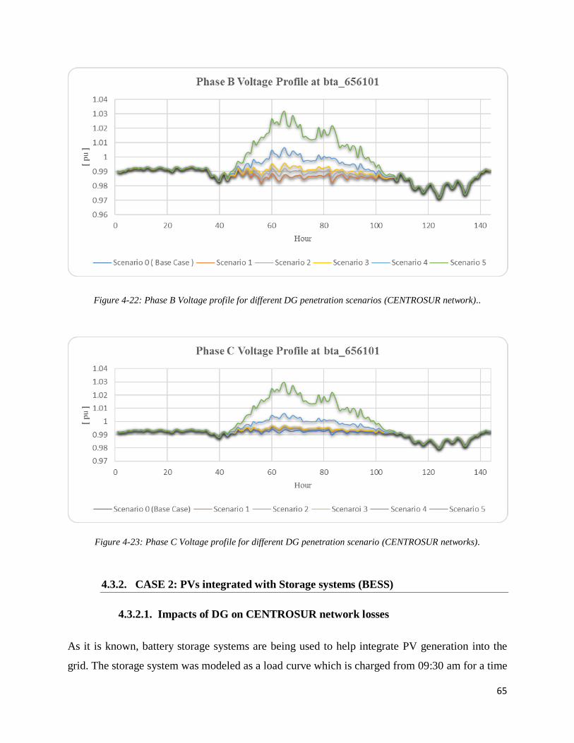
65
Figure 4-22: Phase B Voltage profile for different DG penetration scenarios (CENTROSUR network)..
Figure 4-23: Phase C Voltage profile for different DG penetration scenario (CENTROSUR networks).
4.3.2. CASE 2: PVs integrated with Storage systems (BESS)
4.3.2.1. Impacts of DG on CENTROSUR network losses
As it is known, battery storage systems are being used to help integrate PV generation into the
grid. The storage system was modeled as a load curve which is charged from 09:30 am for a time
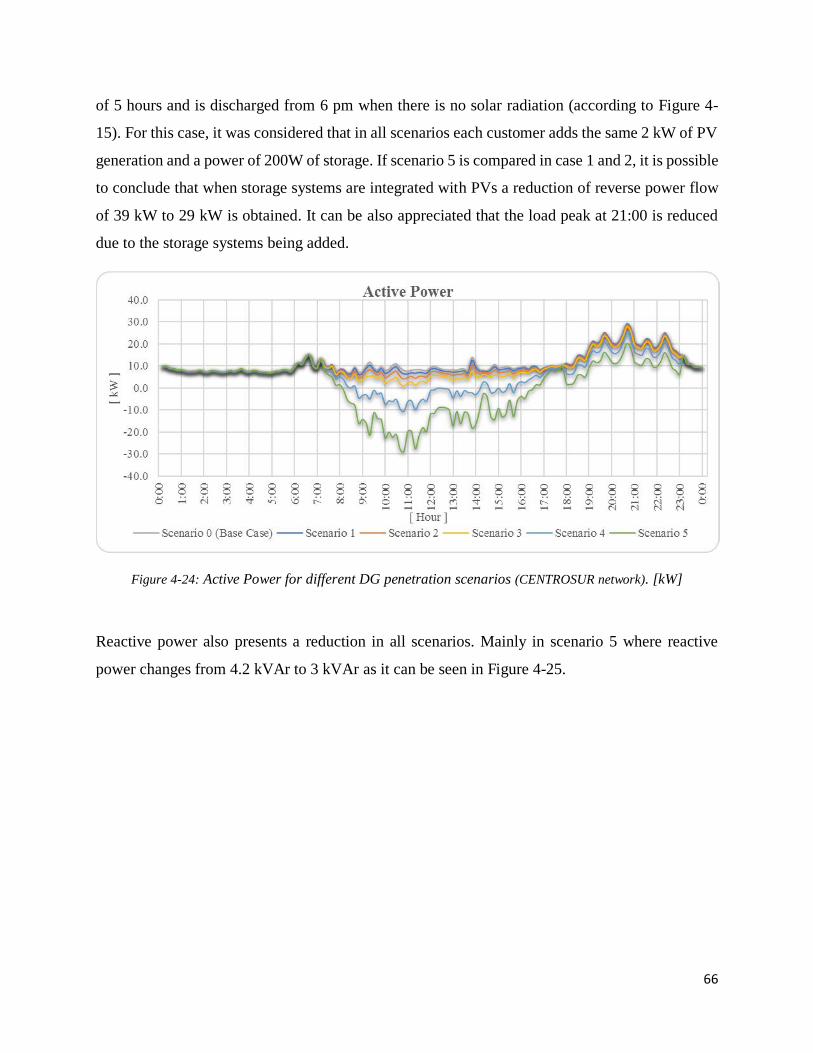
66
of 5 hours and is discharged from 6 pm when there is no solar radiation (according to Figure 4-
15). For this case, it was considered that in all scenarios each customer adds the same 2 kW of PV
generation and a power of 200W of storage. If scenario 5 is compared in case 1 and 2, it is possible
to conclude that when storage systems are integrated with PVs a reduction of reverse power flow
of 39 kW to 29 kW is obtained. It can be also appreciated that the load peak at 21:00 is reduced
due to the storage systems being added.
Figure 4-24: Active Power for different DG penetration scenarios (CENTROSUR network). [kW]
Reactive power also presents a reduction in all scenarios. Mainly in scenario 5 where reactive
power changes from 4.2 kVAr to 3 kVAr as it can be seen in Figure 4-25.
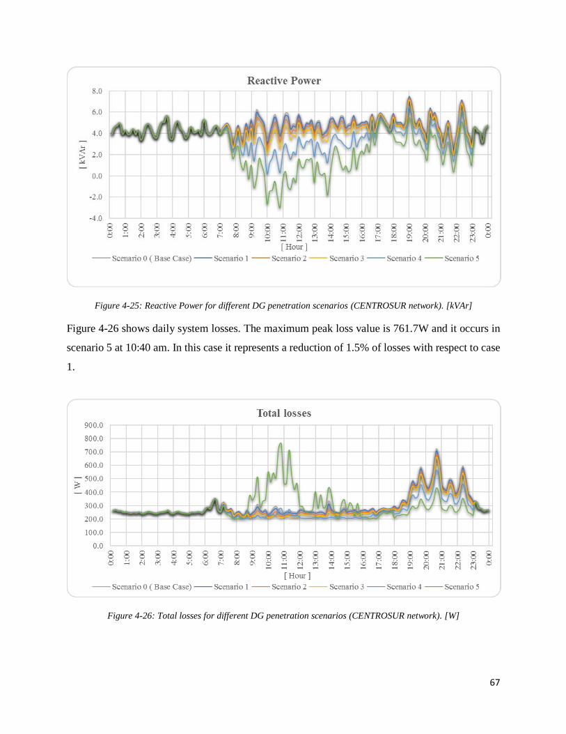
67
Figure 4-25: Reactive Power for different DG penetration scenarios (CENTROSUR network). [kVAr]
Figure 4-26 shows daily system losses. The maximum peak loss value is 761.7W and it occurs in
scenario 5 at 10:40 am. In this case it represents a reduction of 1.5% of losses with respect to case
1.
Figure 4-26: Total losses for different DG penetration scenarios (CENTROSUR network). [W]
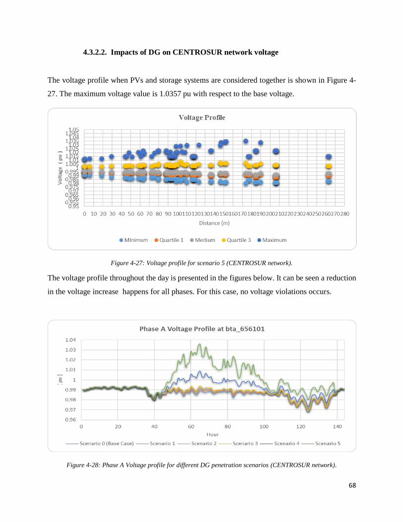
68
4.3.2.2. Impacts of DG on CENTROSUR network voltage
The voltage profile when PVs and storage systems are considered together is shown in Figure 4-
27. The maximum voltage value is 1.0357 pu with respect to the base voltage.
Figure 4-27: Voltage profile for scenario 5 (CENTROSUR network).
The voltage profile throughout the day is presented in the figures below. It can be seen a reduction
in the voltage increase happens for all phases. For this case, no voltage violations occurs.
Figure 4-28: Phase A Voltage profile for different DG penetration scenarios (CENTROSUR network).
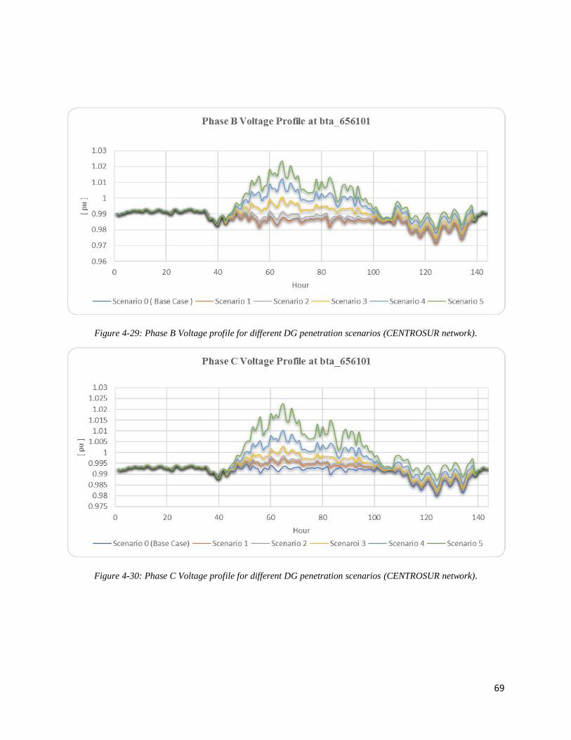
69
Figure 4-29: Phase B Voltage profile for different DG penetration scenarios (CENTROSUR network).
Figure 4-30: Phase C Voltage profile for different DG penetration scenarios (CENTROSUR network).
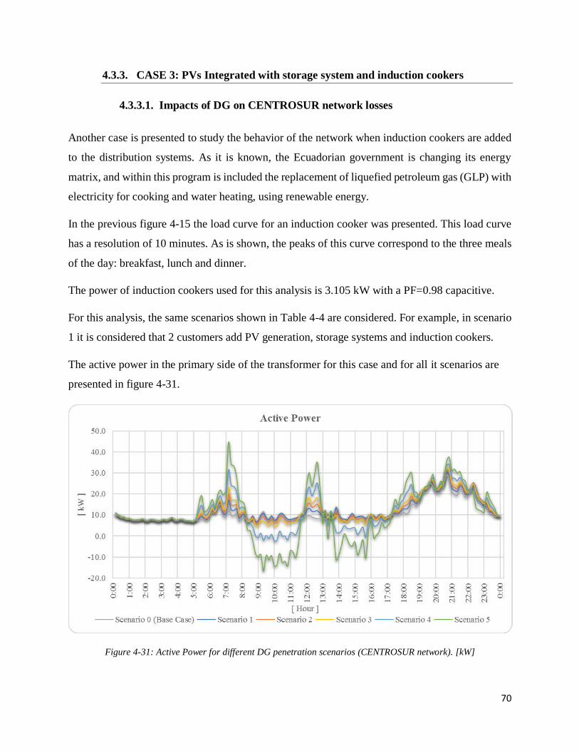
70
4.3.3. CASE 3: PVs Integrated with storage system and induction cookers
4.3.3.1. Impacts of DG on CENTROSUR network losses
Another case is presented to study the behavior of the network when induction cookers are added
to the distribution systems. As it is known, the Ecuadorian government is changing its energy
matrix, and within this program is included the replacement of liquefied petroleum gas (GLP) with
electricity for cooking and water heating, using renewable energy.
In the previous figure 4-15 the load curve for an induction cooker was presented. This load curve
has a resolution of 10 minutes. As is shown, the peaks of this curve correspond to the three meals
of the day: breakfast, lunch and dinner.
The power of induction cookers used for this analysis is 3.105 kW with a PF=0.98 capacitive.
For this analysis, the same scenarios shown in Table 4-4 are considered. For example, in scenario
1 it is considered that 2 customers add PV generation, storage systems and induction cookers.
The active power in the primary side of the transformer for this case and for all it scenarios are
presented in figure 4-31.
Figure 4-31: Active Power for different DG penetration scenarios (CENTROSUR network). [kW]
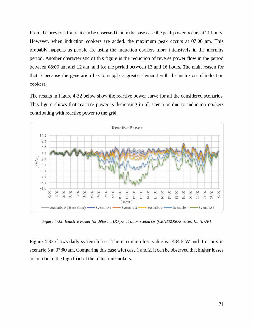
71
From the previous figure it can be observed that in the base case the peak power occurs at 21 hours.
However, when induction cookers are added, the maximum peak occurs at 07:00 am. This
probably happens as people are using the induction cookers more intensively in the morning
period. Another characteristic of this figure is the reduction of reverse power flow in the period
between 08:00 am and 12 am, and for the period between 13 and 16 hours. The main reason for
that is because the generation has to supply a greater demand with the inclusion of induction
cookers.
The results in Figure 4-32 below show the reactive power curve for all the considered scenarios.
This figure shows that reactive power is decreasing in all scenarios due to induction cookers
contributing with reactive power to the grid.
Figure 4-32: Reactive Power for different DG penetration scenarios (CENTROSUR network). [kVAr]
Figure 4-33 shows daily system losses. The maximum loss value is 1434.6 W and it occurs in
scenario 5 at 07:00 am. Comparing this case with case 1 and 2, it can be observed that higher losses
occur due to the high load of the induction cookers.
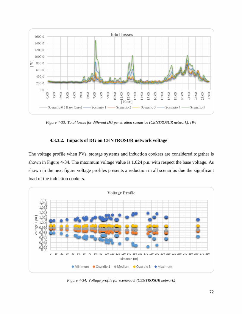
72
Figure 4-33: Total losses for different DG penetration scenarios (CENTROSUR network). [W]
4.3.3.2. Impacts of DG on CENTROSUR network voltage
The voltage profile when PVs, storage systems and induction cookers are considered together is
shown in Figure 4-34. The maximum voltage value is 1.024 p.u. with respect the base voltage. As
shown in the next figure voltage profiles presents a reduction in all scenarios due the significant
load of the induction cookers.
Figure 4-34: Voltage profile for scenario 5 (CENTROSUR network)
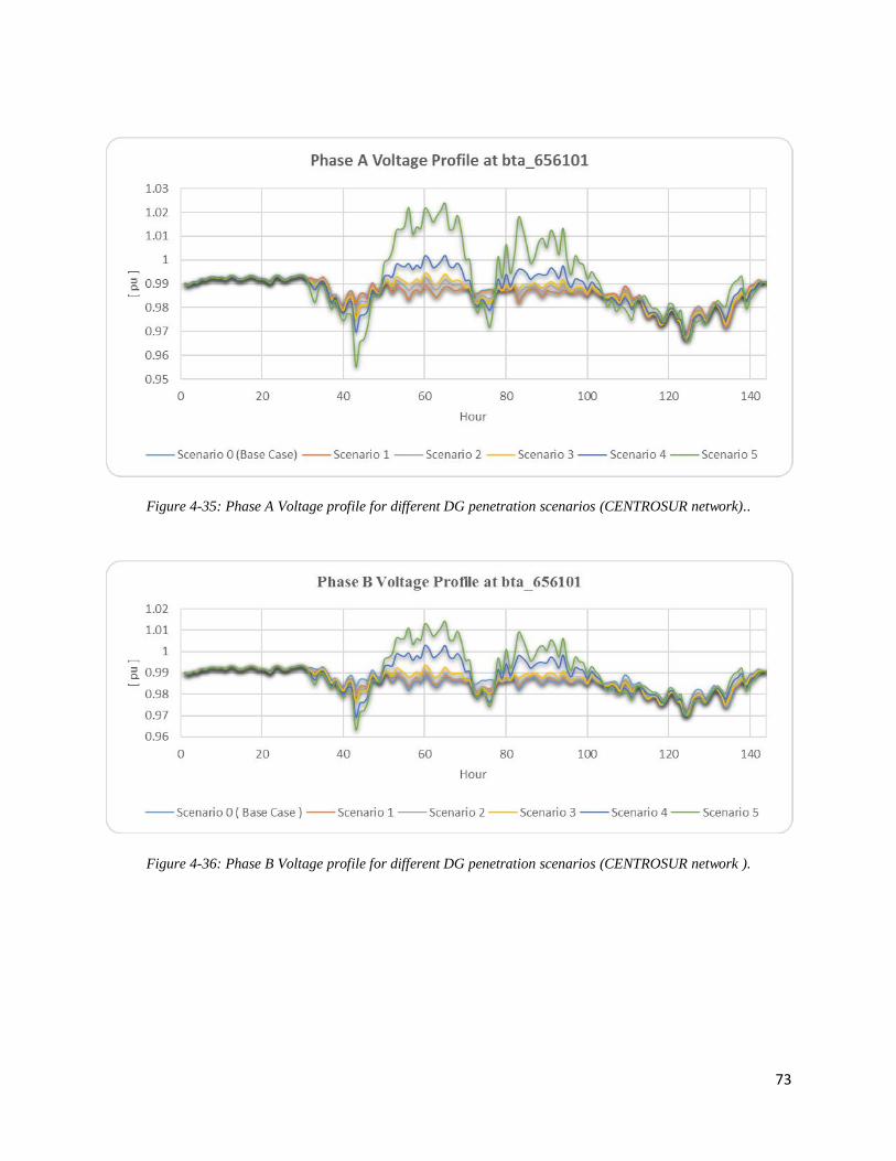
73
Figure 4-35: Phase A Voltage profile for different DG penetration scenarios (CENTROSUR network)..
Figure 4-36: Phase B Voltage profile for different DG penetration scenarios (CENTROSUR network ).
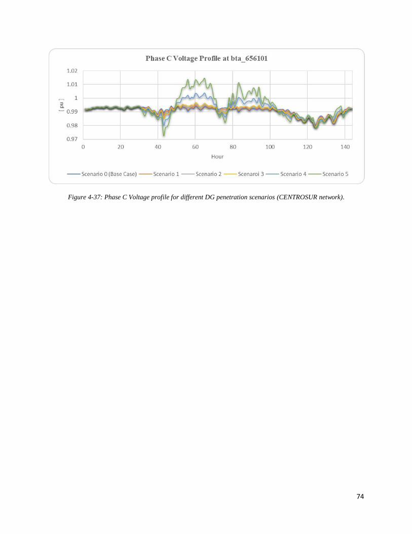
74
Figure 4-37: Phase C Voltage profile for different DG penetration scenarios (CENTROSUR network).
75
5. CONCLUSIONS:
Today with the increasing installation of PV with energy storage systems, electricity distribution
utilities are carrying out analysis to know the affected grid parameters when a customer decides to
connect DG to the grid. This analysis focus into many areas such as voltage regulation, grid
stability, fault detection, dynamic control, power quality, etc. However, this thesis focused on,
studying the effect of grid-connected PV generation with storage and also with induction cookers
on technical parameter such as losses, voltage profile and reverse power. As for the most important
conclusions obtained, it can be said that:
For IEEE 13 buses feeder, simulation results showed that better result in the voltage profile and
losses are obtained when the same amount of DG is connected to specific buses where the load is
highly, and no at all buses. Another approach called QSTS was adopted due to this analysis it is
possible to determine technical characteristics of the network along one day, one month, or one
year, particularly when a large amount of PV generation is added in hours where the demand is
light. However, once this simulation mode is carried out, a little bit improvement could be seen in
profile voltage along the day, particularly in hours where there is solar radiation.
The QSTS results for CENTROSUR network showed that there are no reversed power flow
problems for the three scenarios when only PV generation is considered. On the other hand, results
show a reversal of active power flow from the customer back to the transformer with 50% (scenario
4) accumulated PV connection during a day. High losses take place due to this reversed power
flow. The maximum loss value is 1156.35W, and it occurs in scenario 5. If scenario 0 and 5 are
compared, it can be shown that losses increased a value of 434.32W.
With the purpose of reducing losses and the reverse power flow another study case is presented.
In this case, battery storage systems were integrated with PV generation. The results show that if
scenario 5 is compared in case 1 (only PV) and case 2 ( PV+BESS) a reduction of reverse power
flow of 39 kW to 29 kW is obtained. It can also be appreciated that the load peak is reduced in all
scenarios due to the storage systems being added. For this case, the maximum losses value is 761.7
W, which represents an increase of 39.64 W with respect to base case where losses are 722.02 W

76
For the analysis of the real network it was considered that each customer adds a maximum power
of 2 kW. Above this limit, there would be violations on the voltage levels. Another reason
considered to simulate with a power of 2kW is due to the space that would be needed for the
installation of by each client.
In terms of software it can be said that OpenDSS presents obvious advantages. It software allows
to carry out solutions such as snapshot type and quasi-static time series. One of the high point of
OpenDSS is that it can be handled by programs like Microsoft VBA allowing this way for example
to perform programs for optimization. On the other hand OpenDSS has an unfriendly graphical
environment which makes learning a little difficult.
77
FUTURE WORKS
• In this work, only the impacts of PV generation and storage systems in the distribution
network was analyzed. As a future work it should be analyzed the impact of new
technologies and distributed resources such as electric vehicles, wind turbines, electric heat
pumps, etc. In the case of electric vehicles, they could be used as a storage source for PV
generation and can be used to supply energy when solar radiation being null.
• Another interesting work it would be to work with hundreds of circuits to have more
generalized conclusions and with more confidence.
• In the literature review there are very few studies that perform transient analysis in
distribution networks so an interesting analysis would be to carry out the transient analysis
of the impact of DG in electrical distribution network.
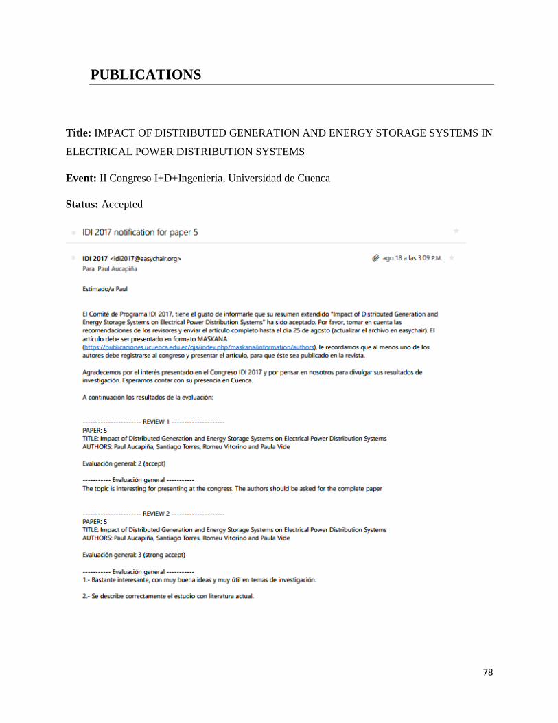
78
PUBLICATIONS
Title: IMPACT OF DISTRIBUTED GENERATION AND ENERGY STORAGE SYSTEMS IN
ELECTRICAL POWER DISTRIBUTION SYSTEMS
Event: II Congreso I+D+Ingenieria, Universidad de Cuenca
Status: Accepted
79
BIBLIOGRAPHY:
[1] R. Simpson et al., “Distributed Generation and Distributed Storage,” 2014.
[2] IEEE, “Institute of Electrical and Electronics Engineers.” [Online]. Available: http://www.ieee.org.
[3] “Electric Power Research Institute,” Jan-1998. [Online]. Available: http://www.epri.com/gg/newgen/disgen/index.html.
[4] CIGRE, “Impact of increasing contribution of dispersed generation on the power system,” CIGRE Study Commitee, vol. 37, 1998.
[5] D. P. G. Gas Research Institute, “Strategy, A for a Competitive Energy Industry, Gas Research Institute,” Chicago, 1998.
[6] W. El-Khattam and M. M. A. Salama, “Distributed generation technologies, definitions and benefits,” Electr. Power Syst. Res., vol. 71, no. 2, pp. 119–128, 2004.
[7] M. Suter, “Active filter for a microturbine,” in Proceedings of the Telecommunications Energy Conference, 2001, pp. 162–165.
[8] M. Elbuluk, “The Role Power Electronics in Future Energy Systems and Green Industrialization,” Power, no. PECon 08, pp. 1–6, 2008.
[9] B. Lasseter, “Microgrids (distributed power generation),” Proc. Power Eng. Soc. Winter Meet. IEEE, vol. 1, pp. 146–149, 2001.
[10] M. W. Ellis and M.R Von Spakovsky, “Fuell cell systems: efficient, felxible energy conversion for the 21 st century,” Proceedings of the IEEE, vol. 89, pp. 1808–1818, 2001.
[11] M. Farooque and H. C. Maru, “Fuel cells—the clean and efficient power generators,” vol. 89, no. 12, pp. 1819–1829, 2001.
[12] A. Borbely and J. F. Kreider, Distributed Generation The Power Paradigm for the New Millennium, 2001 CRC. Washington.
[13] IEC, “Electrical Energy Storage - White Paper,” Int. Electrotech. Comm., pp. 1–78, 2011.
[14] E. Barbour, “Pumped Hydroelectric Storage (PHS).” [Online]. Available: http://energystoragesense.com/pumped-hydroelectric-storage-phs/. [Accessed: 01-Jan-2017].
[15] “Discover renewable energy technology with compressed air energy storage.” [Online]. Available: https://www.pge.com/en_US/about-pge. [Accessed: 01-Jan-2017].
[16] “Integration of Facts Into Energy Storage Systems for Future Power,” vol. 2, no. 2, pp. 800–810, 2013.
[17] Mukund R. Patel, Wind and Solar Power Systems: Design, Analysis, and Operation, Second. 2006.
[18] E. KInnab, “Study About Wind Turbines.” [Online]. Available: https://www.slideshare.net/eliatohme/study-about-wind-turbines. [Accessed: 01-Jan-2017].
[19] Y. Baghzouz, “General rules for distributed generation - feeder interaction,” Power Eng. Soc. Gen. Meet., vol. 4, pp. 18–22, 2006.
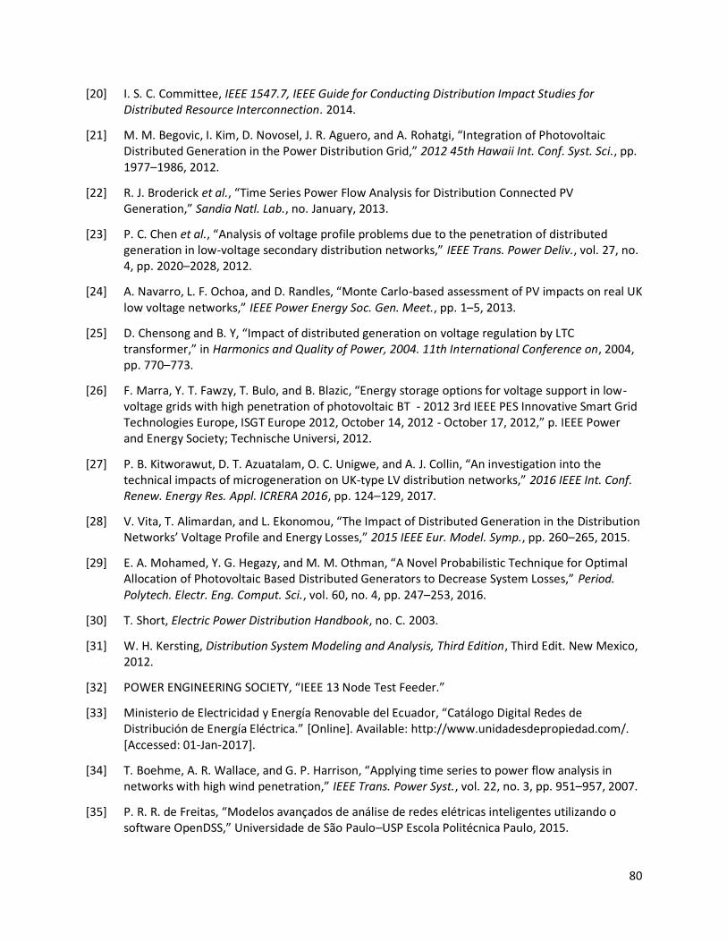
80
[20] I. S. C. Committee, IEEE 1547.7, IEEE Guide for Conducting Distribution Impact Studies for Distributed Resource Interconnection. 2014.
[21] M. M. Begovic, I. Kim, D. Novosel, J. R. Aguero, and A. Rohatgi, “Integration of Photovoltaic Distributed Generation in the Power Distribution Grid,” 2012 45th Hawaii Int. Conf. Syst. Sci., pp. 1977–1986, 2012.
[22] R. J. Broderick et al., “Time Series Power Flow Analysis for Distribution Connected PV Generation,” Sandia Natl. Lab., no. January, 2013.
[23] P. C. Chen et al., “Analysis of voltage profile problems due to the penetration of distributed generation in low-voltage secondary distribution networks,” IEEE Trans. Power Deliv., vol. 27, no. 4, pp. 2020–2028, 2012.
[24] A. Navarro, L. F. Ochoa, and D. Randles, “Monte Carlo-based assessment of PV impacts on real UK low voltage networks,” IEEE Power Energy Soc. Gen. Meet., pp. 1–5, 2013.
[25] D. Chensong and B. Y, “Impact of distributed generation on voltage regulation by LTC transformer,” in Harmonics and Quality of Power, 2004. 11th International Conference on, 2004, pp. 770–773.
[26] F. Marra, Y. T. Fawzy, T. Bulo, and B. Blazic, “Energy storage options for voltage support in low-voltage grids with high penetration of photovoltaic BT - 2012 3rd IEEE PES Innovative Smart Grid Technologies Europe, ISGT Europe 2012, October 14, 2012 - October 17, 2012,” p. IEEE Power and Energy Society; Technische Universi, 2012.
[27] P. B. Kitworawut, D. T. Azuatalam, O. C. Unigwe, and A. J. Collin, “An investigation into the technical impacts of microgeneration on UK-type LV distribution networks,” 2016 IEEE Int. Conf. Renew. Energy Res. Appl. ICRERA 2016, pp. 124–129, 2017.
[28] V. Vita, T. Alimardan, and L. Ekonomou, “The Impact of Distributed Generation in the Distribution Networks’ Voltage Profile and Energy Losses,” 2015 IEEE Eur. Model. Symp., pp. 260–265, 2015.
[29] E. A. Mohamed, Y. G. Hegazy, and M. M. Othman, “A Novel Probabilistic Technique for Optimal Allocation of Photovoltaic Based Distributed Generators to Decrease System Losses,” Period. Polytech. Electr. Eng. Comput. Sci., vol. 60, no. 4, pp. 247–253, 2016.
[30] T. Short, Electric Power Distribution Handbook, no. C. 2003.
[31] W. H. Kersting, Distribution System Modeling and Analysis, Third Edition, Third Edit. New Mexico, 2012.
[32] POWER ENGINEERING SOCIETY, “IEEE 13 Node Test Feeder.”
[33] Ministerio de Electricidad y Energía Renovable del Ecuador, “Catálogo Digital Redes de Distribución de Energía Eléctrica.” [Online]. Available: http://www.unidadesdepropiedad.com/. [Accessed: 01-Jan-2017].
[34] T. Boehme, A. R. Wallace, and G. P. Harrison, “Applying time series to power flow analysis in networks with high wind penetration,” IEEE Trans. Power Syst., vol. 22, no. 3, pp. 951–957, 2007.
[35] P. R. R. de Freitas, “Modelos avançados de análise de redes elétricas inteligentes utilizando o software OpenDSS,” Universidade de São Paulo–USP Escola Politécnica Paulo, 2015.
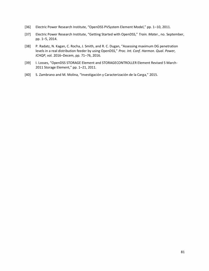
81
[36] Electric Power Research Institute, “OpenDSS PVSystem Element Model,” pp. 1–10, 2011.
[37] Electric Power Research Institute, “Getting Started with OpenDSS,” Train. Mater., no. September, pp. 1–5, 2014.
[38] P. Radatz, N. Kagan, C. Rocha, J. Smith, and R. C. Dugan, “Assessing maximum DG penetration levels in a real distribution feeder by using OpenDSS,” Proc. Int. Conf. Harmon. Qual. Power, ICHQP, vol. 2016–Decem, pp. 71–76, 2016.
[39] I. Losses, “OpenDSS STORAGE Element and STORAGECONTROLLER Element Revised 5 March-2011 Storage Element,” pp. 1–21, 2011.
[40] S. Zambrano and M. Molina, “Investigación y Caracterización de la Carga,” 2015.
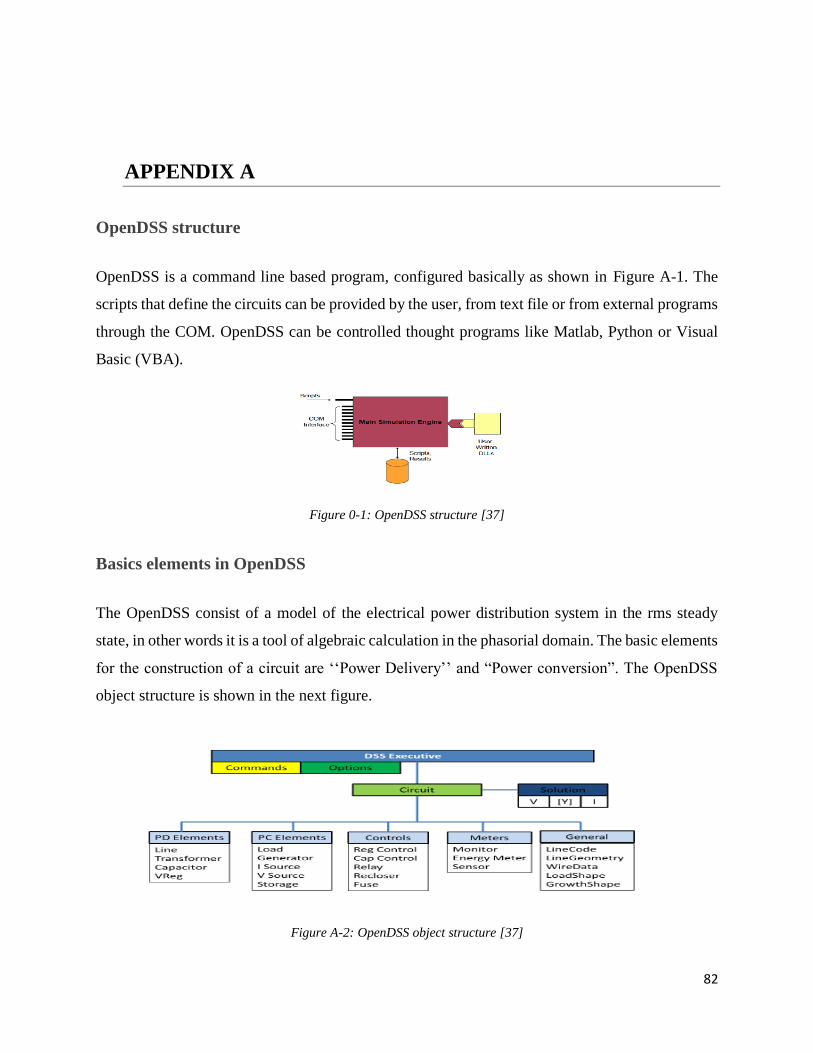
82
APPENDIX A
OpenDSS structure
OpenDSS is a command line based program, configured basically as shown in Figure A-1. The
scripts that define the circuits can be provided by the user, from text file or from external programs
through the COM. OpenDSS can be controlled thought programs like Matlab, Python or Visual
Basic (VBA).
Figure 0-1: OpenDSS structure [37]
Basics elements in OpenDSS
The OpenDSS consist of a model of the electrical power distribution system in the rms steady
state, in other words it is a tool of algebraic calculation in the phasorial domain. The basic elements
for the construction of a circuit are ‘‘Power Delivery’’ and “Power conversion”. The OpenDSS
object structure is shown in the next figure.
Figure A-2: OpenDSS object structure [37]
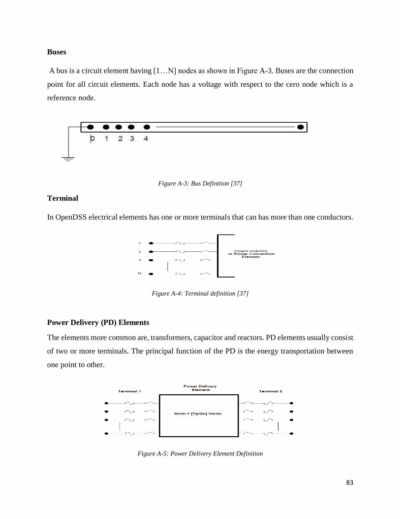
83
Buses
A bus is a circuit element having [1…N] nodes as shown in Figure A-3. Buses are the connection
point for all circuit elements. Each node has a voltage with respect to the cero node which is a
reference node.
Figure A-3: Bus Definition [37]
Terminal
In OpenDSS electrical elements has one or more terminals that can has more than one conductors.
Figure A-4: Terminal definition [37]
Power Delivery (PD) Elements
The elements more common are, transformers, capacitor and reactors. PD elements usually consist
of two or more terminals. The principal function of the PD is the energy transportation between
one point to other.
Figure A-5: Power Delivery Element Definition
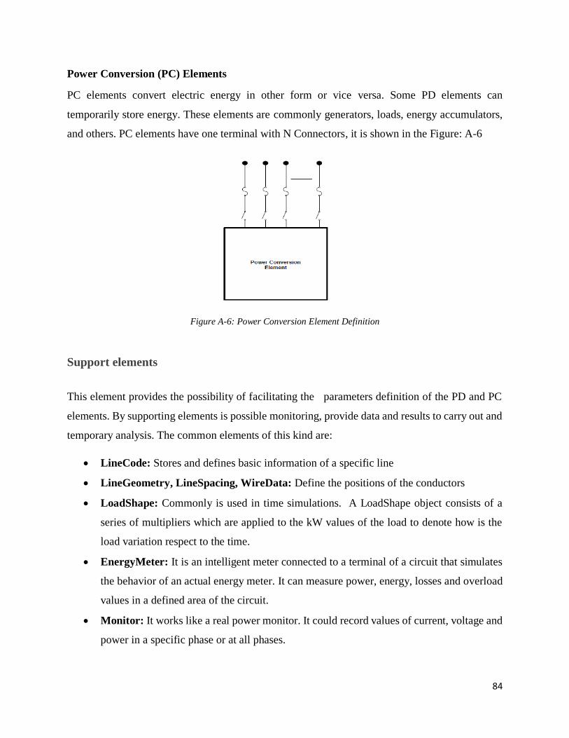
84
Power Conversion (PC) Elements
PC elements convert electric energy in other form or vice versa. Some PD elements can
temporarily store energy. These elements are commonly generators, loads, energy accumulators,
and others. PC elements have one terminal with N Connectors, it is shown in the Figure: A-6
Figure A-6: Power Conversion Element Definition
Support elements
This element provides the possibility of facilitating the parameters definition of the PD and PC
elements. By supporting elements is possible monitoring, provide data and results to carry out and
temporary analysis. The common elements of this kind are:
• LineCode: Stores and defines basic information of a specific line
• LineGeometry, LineSpacing, WireData: Define the positions of the conductors
• LoadShape: Commonly is used in time simulations. A LoadShape object consists of a
series of multipliers which are applied to the kW values of the load to denote how is the
load variation respect to the time.
• EnergyMeter: It is an intelligent meter connected to a terminal of a circuit that simulates
the behavior of an actual energy meter. It can measure power, energy, losses and overload
values in a defined area of the circuit.
• Monitor: It works like a real power monitor. It could record values of current, voltage and
power in a specific phase or at all phases.
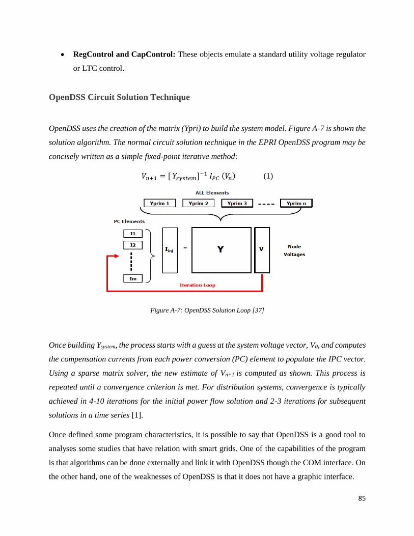
85
• RegControl and CapControl: These objects emulate a standard utility voltage regulator
or LTC control.
OpenDSS Circuit Solution Technique
OpenDSS uses the creation of the matrix (Ypri) to build the system model. Figure A-7 is shown the
solution algorithm. The normal circuit solution technique in the EPRI OpenDSS program may be
concisely written as a simple fixed-point iterative method:
𝑉𝑛+1 = [ 𝑌𝑠𝑦𝑠𝑡𝑒𝑚]−1 𝐼𝑃𝐶 (𝑉𝑛) (1)
Figure A-7: OpenDSS Solution Loop [37]
Once building Ysystem, the process starts with a guess at the system voltage vector, V0, and computes
the compensation currents from each power conversion (PC) element to populate the IPC vector.
Using a sparse matrix solver, the new estimate of Vn+1 is computed as shown. This process is
repeated until a convergence criterion is met. For distribution systems, convergence is typically
achieved in 4-10 iterations for the initial power flow solution and 2-3 iterations for subsequent
solutions in a time series [1].
Once defined some program characteristics, it is possible to say that OpenDSS is a good tool to
analyses some studies that have relation with smart grids. One of the capabilities of the program
is that algorithms can be done externally and link it with OpenDSS though the COM interface. On
the other hand, one of the weaknesses of OpenDSS is that it does not have a graphic interface.

86
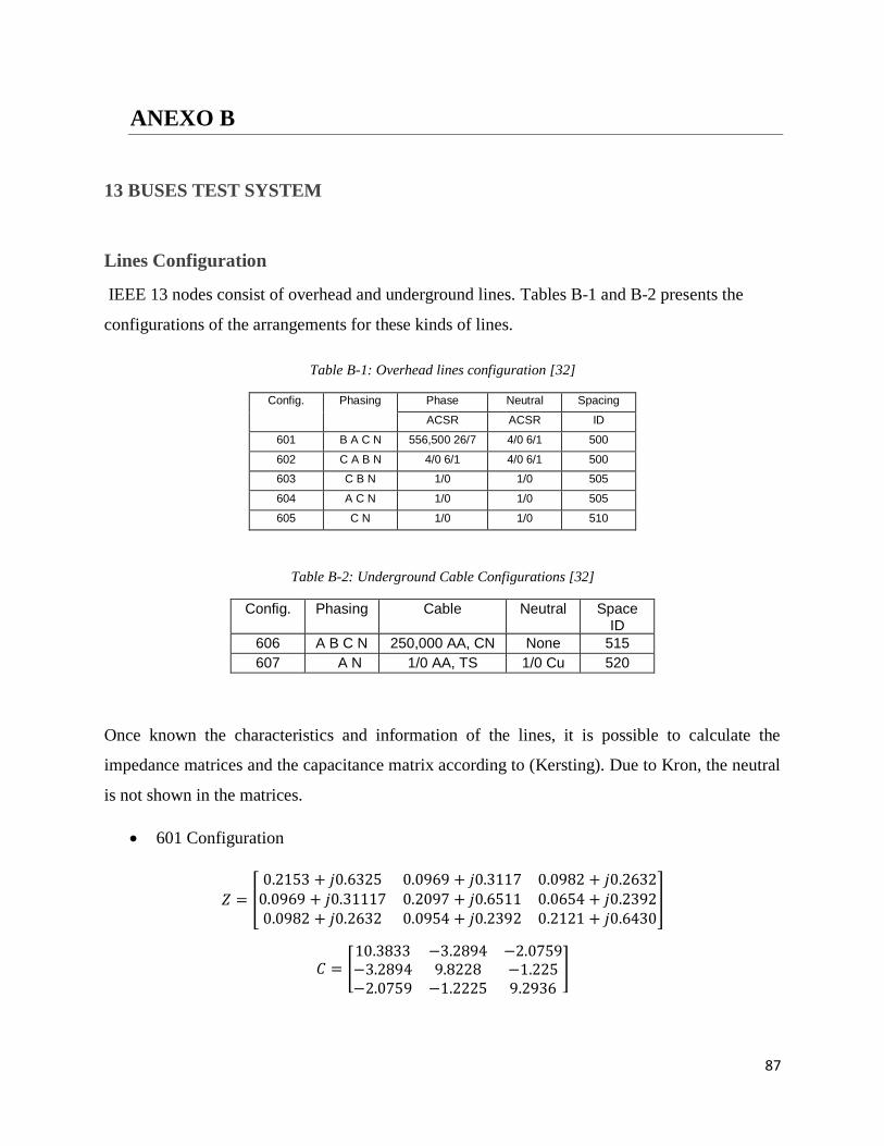
87
ANEXO B
13 BUSES TEST SYSTEM
Lines Configuration
IEEE 13 nodes consist of overhead and underground lines. Tables B-1 and B-2 presents the
configurations of the arrangements for these kinds of lines.
Table B-1: Overhead lines configuration [32]
Config. Phasing Phase Neutral Spacing
ACSR ACSR ID
601 B A C N 556,500 26/7 4/0 6/1 500
602 C A B N 4/0 6/1 4/0 6/1 500
603 C B N 1/0 1/0 505
604 A C N 1/0 1/0 505
605 C N 1/0 1/0 510
Table B-2: Underground Cable Configurations [32]
Config. Phasing Cable Neutral Space ID
606 A B C N 250,000 AA, CN None 515
607 A N 1/0 AA, TS 1/0 Cu 520
Once known the characteristics and information of the lines, it is possible to calculate the
impedance matrices and the capacitance matrix according to (Kersting). Due to Kron, the neutral
is not shown in the matrices.
• 601 Configuration
𝑍 = [
0.2153 + 𝑗0.6325 0.0969 + 𝑗0.3117 0.0982 + 𝑗0.26320.0969 + 𝑗0.31117 0.2097 + 𝑗0.6511 0.0654 + 𝑗0.23920.0982 + 𝑗0.2632 0.0954 + 𝑗0.2392 0.2121 + 𝑗0.6430
]
𝐶 = [10.3833 −3.2894 −2.0759−3.2894 9.8228 −1.225−2.0759 −1.2225 9.2936
]
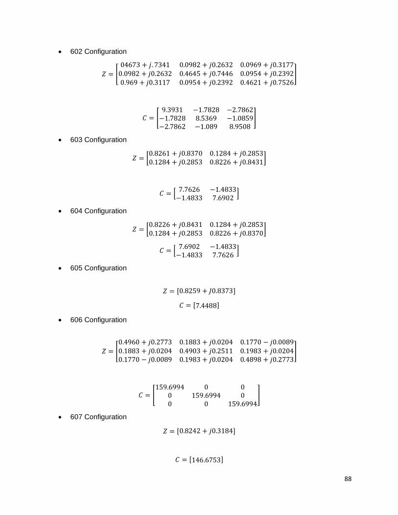
88
• 602 Configuration
𝑍 = [
04673 + 𝑗. 7341 0.0982 + 𝑗0.2632 0.0969 + 𝑗0.31770.0982 + 𝑗0.2632 0.4645 + 𝑗0.7446 0.0954 + 𝑗0.23920.969 + 𝑗0.3117 0.0954 + 𝑗0.2392 0.4621 + 𝑗0.7526
]
𝐶 = [9.3931 −1.7828 −2.7862
−1.7828 8.5369 −1.0859−2.7862 −1.089 8.9508
]
• 603 Configuration
𝑍 = [0.8261 + 𝑗0.8370 0.1284 + 𝑗0.28530.1284 + 𝑗0.2853 0.8226 + 𝑗0.8431
]
𝐶 = [7.7626 −1.4833
−1.4833 7.6902]
• 604 Configuration
𝑍 = [0.8226 + 𝑗0.8431 0.1284 + 𝑗0.28530.1284 + 𝑗0.2853 0.8226 + 𝑗0.8370
]
𝐶 = [7.6902 −1.4833
−1.4833 7.7626]
• 605 Configuration
𝑍 = [0.8259 + 𝐽0.8373]
𝐶 = [7.4488]
• 606 Configuration
𝑍 = [
0.4960 + 𝑗0.2773 0.1883 + 𝑗0.0204 0.1770 − 𝑗0.00890.1883 + 𝑗0.0204 0.4903 + 𝑗0.2511 0.1983 + 𝑗0.02040.1770 − 𝑗0.0089 0.1983 + 𝑗0.0204 0.4898 + 𝑗0.2773
]
𝐶 = [159.6994 0 0
0 159.6994 00 0 159.6994
]
• 607 Configuration
𝑍 = [0.8242 + 𝑗0.3184]
𝐶 = [146.6753]
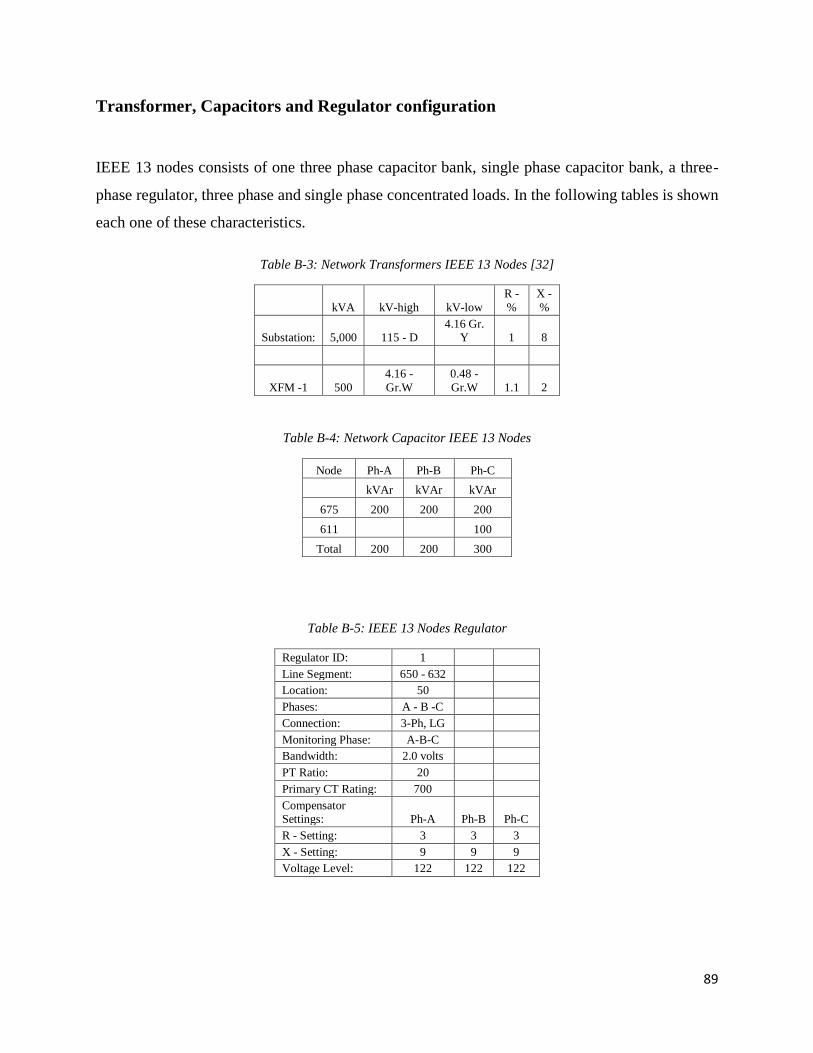
89
Transformer, Capacitors and Regulator configuration
IEEE 13 nodes consists of one three phase capacitor bank, single phase capacitor bank, a three-
phase regulator, three phase and single phase concentrated loads. In the following tables is shown
each one of these characteristics.
Table B-3: Network Transformers IEEE 13 Nodes [32]
kVA kV-high kV-low
R -
%
X -
%
Substation: 5,000 115 - D 4.16 Gr.
Y 1 8
XFM -1 500
4.16 -
Gr.W
0.48 -
Gr.W 1.1 2
Table B-4: Network Capacitor IEEE 13 Nodes
Node Ph-A Ph-B Ph-C
kVAr kVAr kVAr
675 200 200 200
611 100
Total 200 200 300
Table B-5: IEEE 13 Nodes Regulator
Regulator ID: 1
Line Segment: 650 - 632 Location: 50
Phases: A - B -C
Connection: 3-Ph, LG
Monitoring Phase: A-B-C Bandwidth: 2.0 volts
PT Ratio: 20
Primary CT Rating: 700
Compensator Settings: Ph-A Ph-B Ph-C
R - Setting: 3 3 3
X - Setting: 9 9 9
Voltage Level: 122 122 122
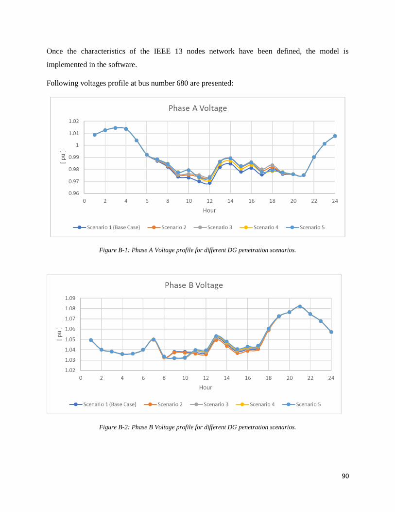
90
Once the characteristics of the IEEE 13 nodes network have been defined, the model is
implemented in the software.
Following voltages profile at bus number 680 are presented:
Figure B-1: Phase A Voltage profile for different DG penetration scenarios.
Figure B-2: Phase B Voltage profile for different DG penetration scenarios.
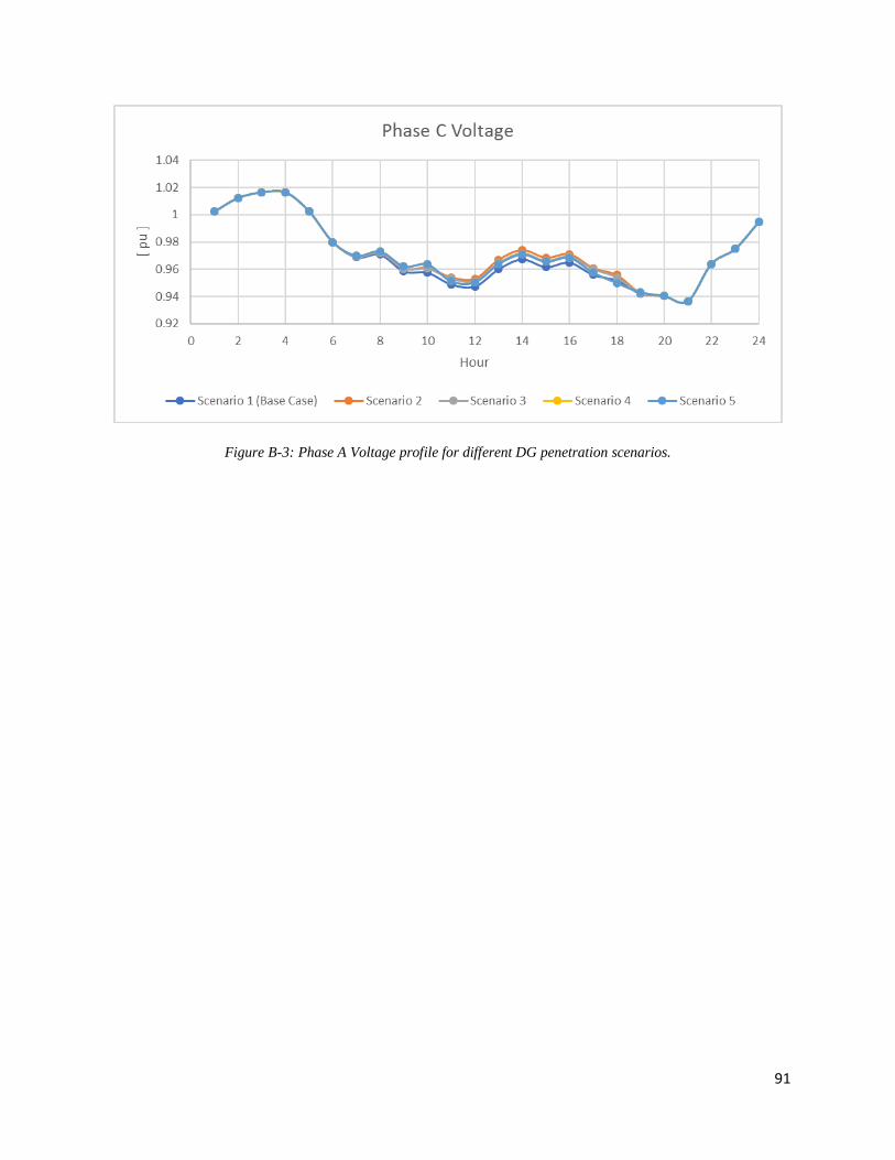
91
Figure B-3: Phase A Voltage profile for different DG penetration scenarios.