Embed Size (px)
Citation preview
Experimental solid mechanics:
Towards the fourth dimension?
Eikology team
MATMECA Seminar, ONERA, Feb. 2016
Tomography
Image materialsTomography
Tomography
Image materials
Image large defects
Image Analysis
Segmentation
Tomography
Image materials
Image motion
Image large defects
Digital Volume
Correlation
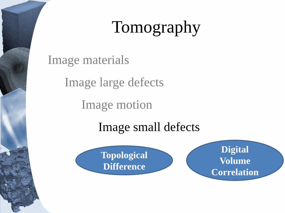
Tomography
Image materials
Image motion
Image small defects
Image large defects
Topological
Difference
Digital
Volume
Correlation
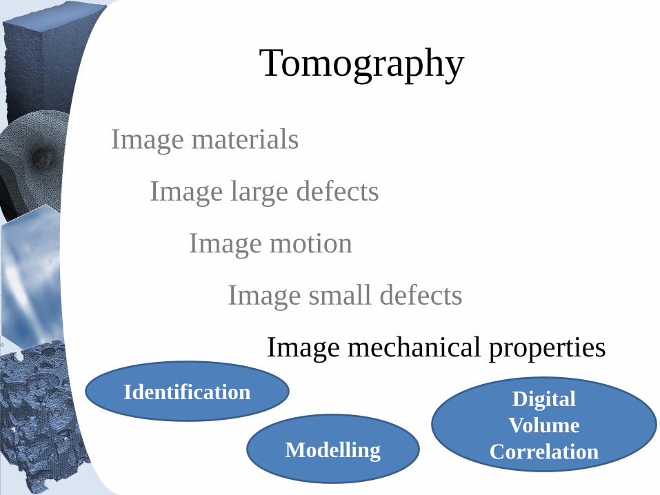
Tomography
Image mechanical properties
Modelling
Image materials
Image motion
Image small defects
Image large defects
Digital
Volume
Correlation
Identification
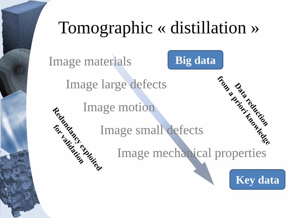
Tomographic « distillation »
Big data
Key data
Image mechanical properties
Image materials
Image motion
Image small defects
Image large defects
Outline
Imaging materials and their
kinematics from in situ testing
From kinematics to mechanics
Perspectives, challenges and
suggestions
Warning: pro domo plea,
but wide open for discussion
IMAGING MATERIALS
& THEIR KINEMATICS
From material science to solid mechanics
Imaging in 3D
• A dream came true
• Essential for Material Science
• Key for industry (NDT & metrology)
• Unavoidable for experimental mechanics!
Wise investment into the future !
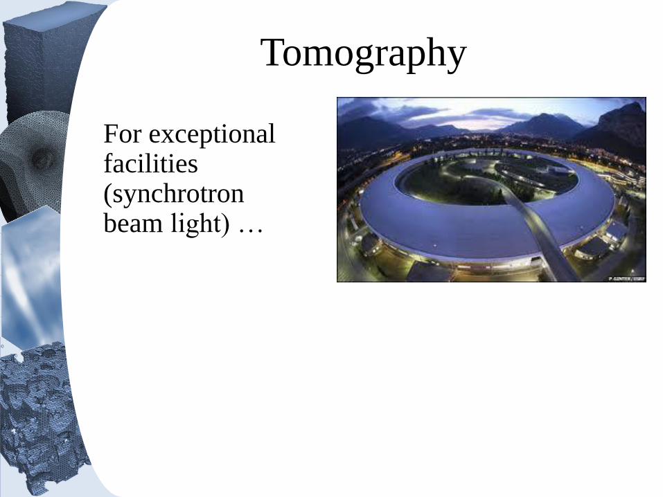
Tomography
For exceptionalfacilities(synchrotron beam light) …
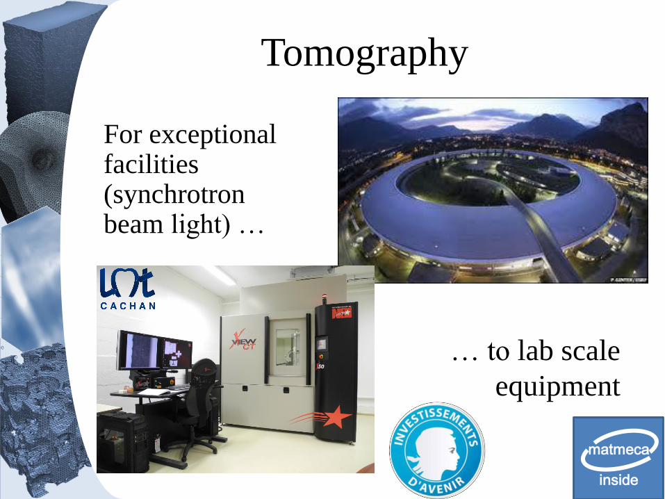
Tomography
… to lab scale
equipment
For exceptionalfacilities(synchrotron beam light) …
inside
matmeca
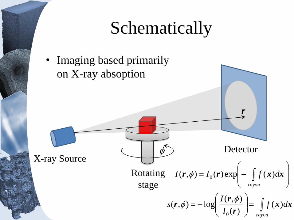
Schematically
• Imaging based primarily
on X-ray absoption
X-ray Source
Rotating
stage
Detector
rayon
dfII xxrr )(exp)(),( 0
rayon
dfI
Is xx
r
rr )(
)(
),(log),(
0
r
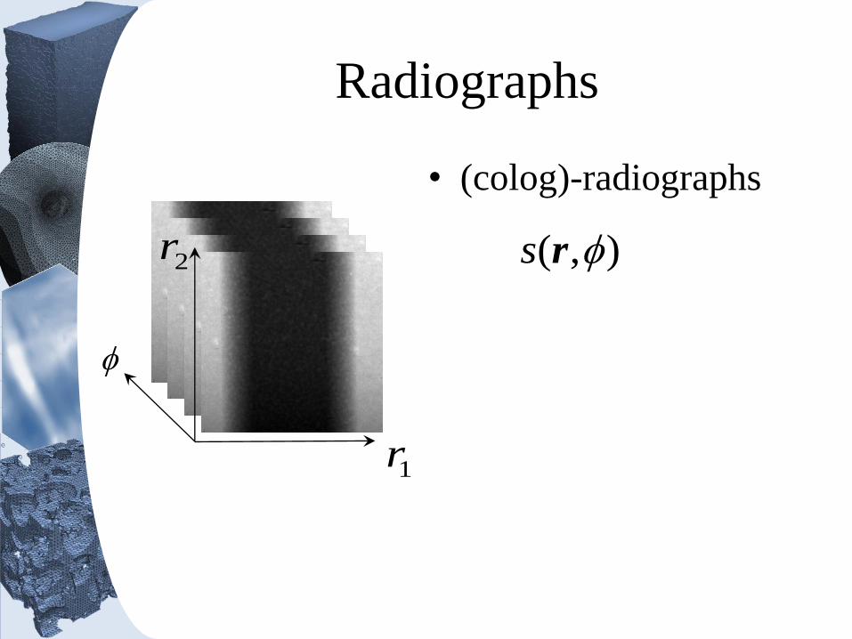
Radiographs
1r
2r ),( rs
• (colog)-radiographs
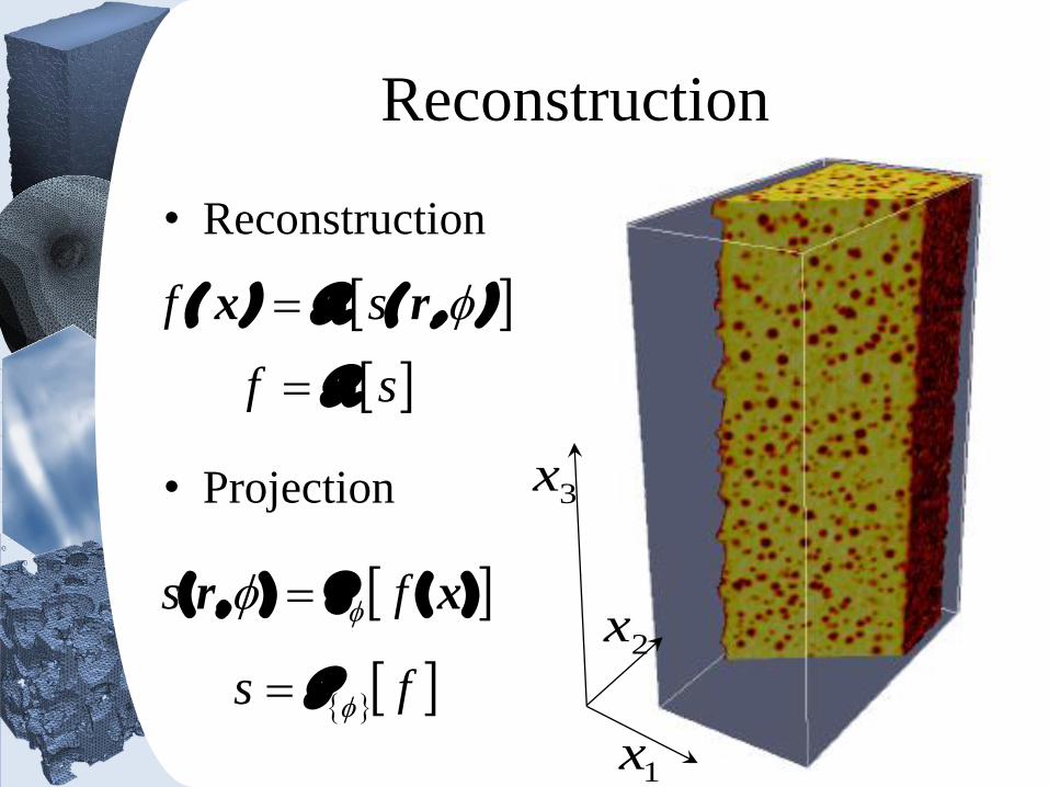
Reconstruction
• Reconstruction
• Projection
1x
2x
3x
),(R)( rx sf
)(P),( xr fs
fs P
sf R
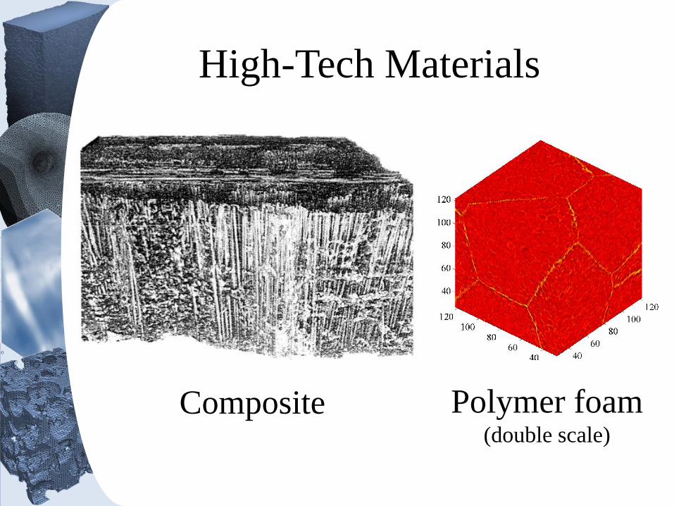
High-Tech Materials
Composite Polymer foam(double scale)
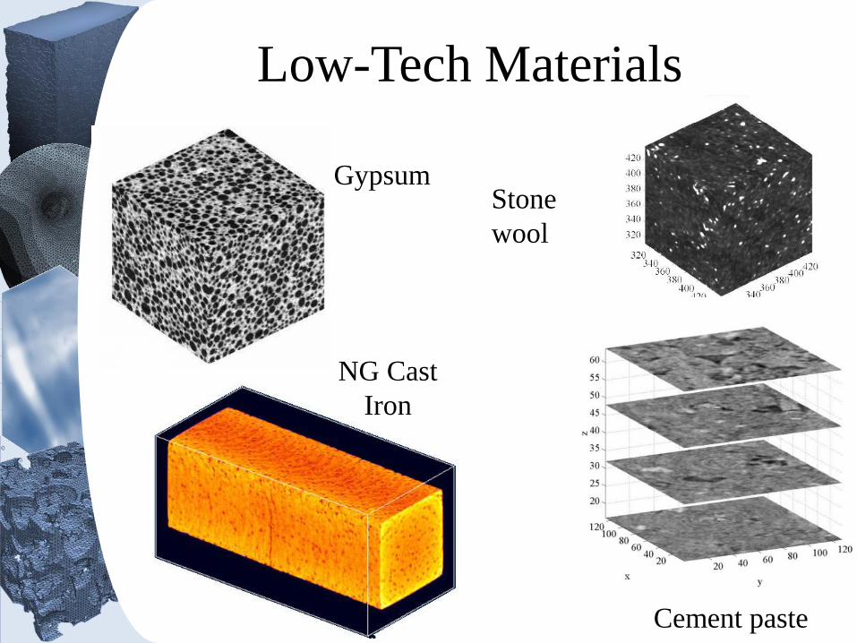
Low-Tech Materials
Gypsum
Cement paste
NG Cast
Iron
Stone
wool
Tomography
• Spectacular progress !
– Spatial resolution
– Temporal resolution
– Wealth of information
– Accessibility
– Data analysis

Perspectives 1
• “Educated” tomographic reconstruction
• Exploitation of non voxel images (e.g. CAD based, reference based, or having a sparse parametrization)
• Instrument development: Phase contrast, or Diffraction contrast
In situ mechanical testing
• Severe constraints …
… that can be overcome !
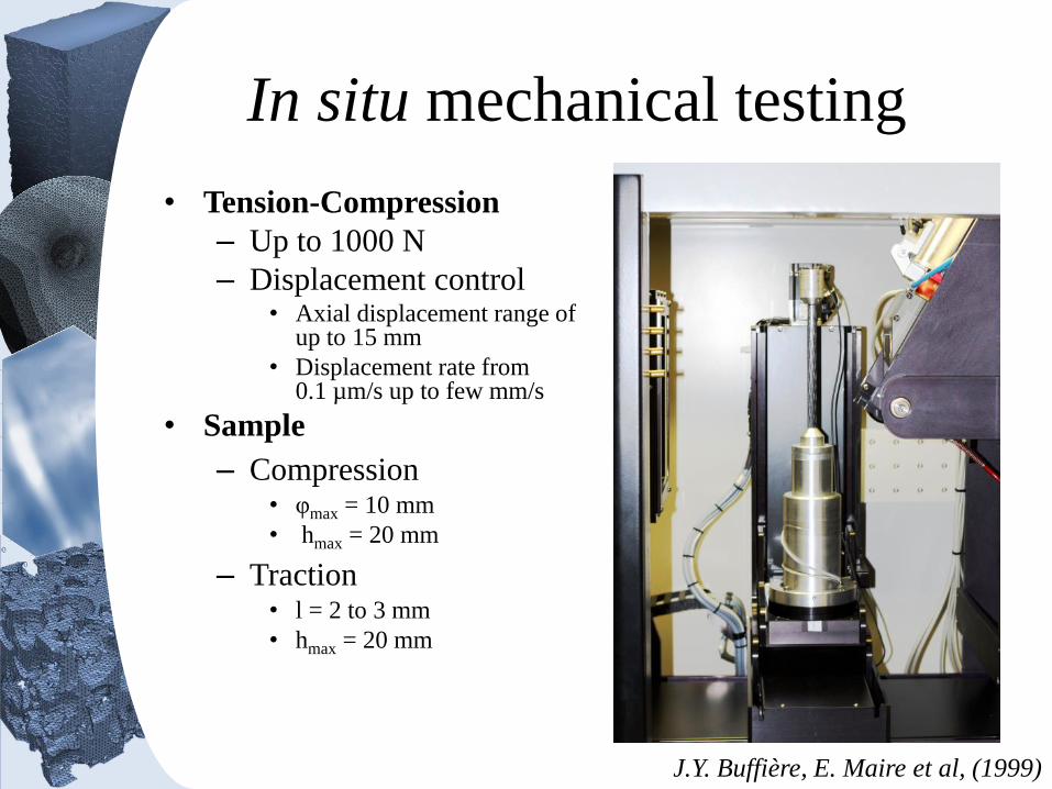
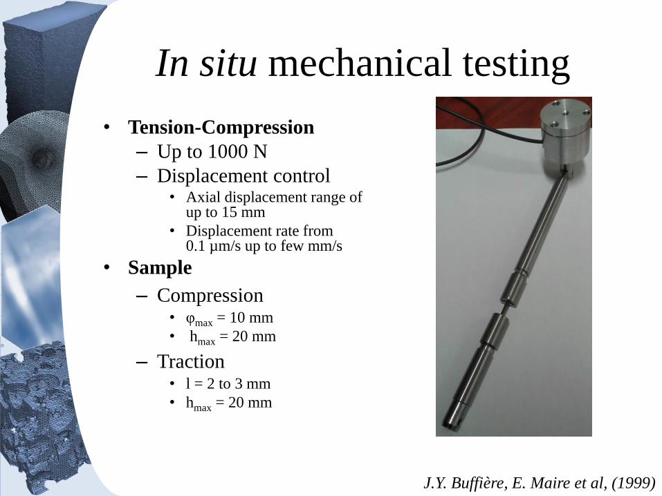
In situ mechanical testing
• Tension-Compression
– Up to 1000 N
– Displacement control• Axial displacement range of
up to 15 mm
• Displacement rate from 0.1 µm/s up to few mm/s
• Sample
– Compression• φmax = 10 mm
• hmax = 20 mm
– Traction• l = 2 to 3 mm
• hmax = 20 mm
J.Y. Buffière, E. Maire et al, (1999)
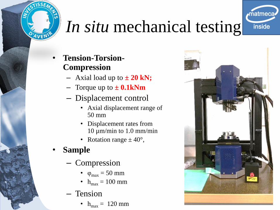
In situ mechanical testing
• Tension-Torsion-Compression
– Axial load up to ± 20 kN;
– Torque up to ± 0.1kNm
– Displacement control• Axial displacement range of
50 mm
• Displacement rates from 10 µm/min to 1.0 mm/min
• Rotation range ± 40°,
• Sample
– Compression• φmax = 50 mm
• hmax = 100 mm
– Tension• hmax = 120 mm
inside
matmeca
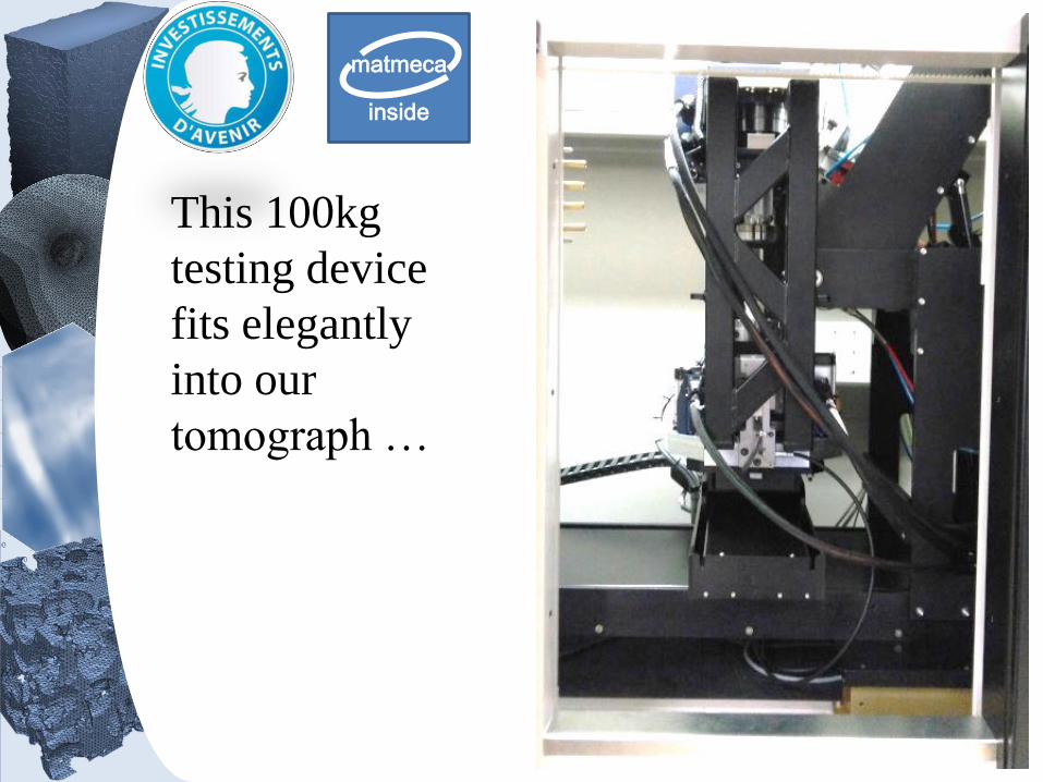
This 100kg
testing device
fits elegantly
into our
tomograph …
inside
matmeca
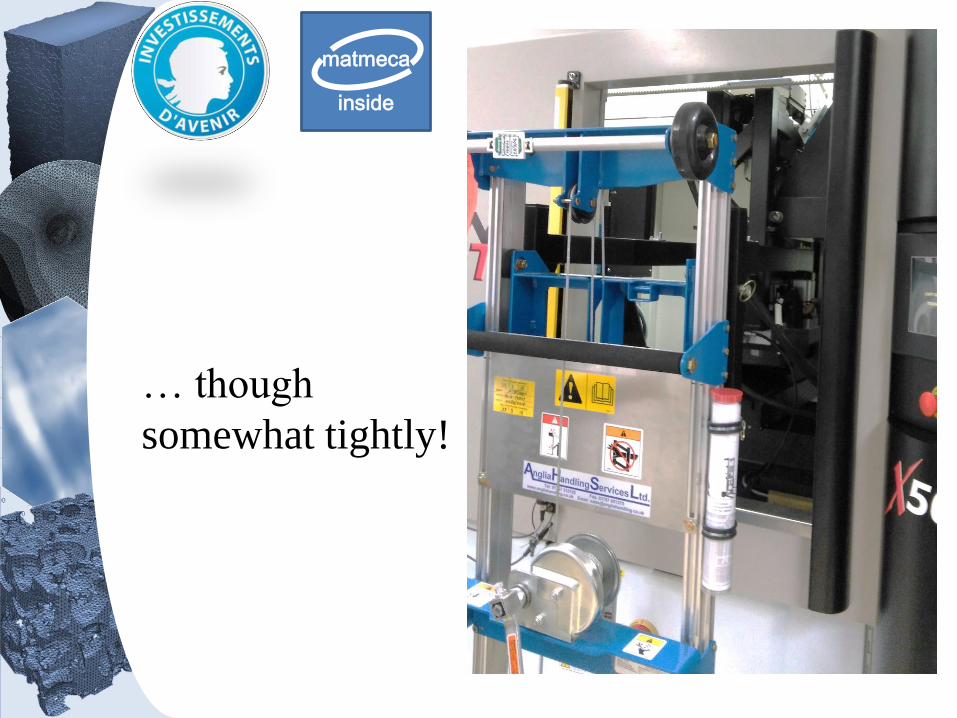
… though
somewhat tightly!
inside
matmeca
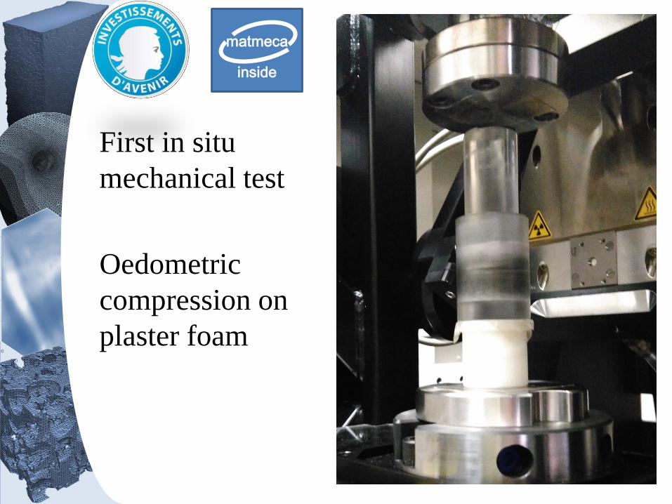
First in situ
mechanical test
Oedometric
compression on
plaster foam
inside
matmeca
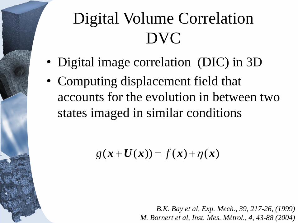
Digital Volume Correlation
DVC
• Digital image correlation (DIC) in 3D
• Computing displacement field that
accounts for the evolution in between two
states imaged in similar conditions
B.K. Bay et al, Exp. Mech., 39, 217-26, (1999)
M. Bornert et al, Inst. Mes. Métrol., 4, 43-88 (2004)
)()())(( xxxUx fg
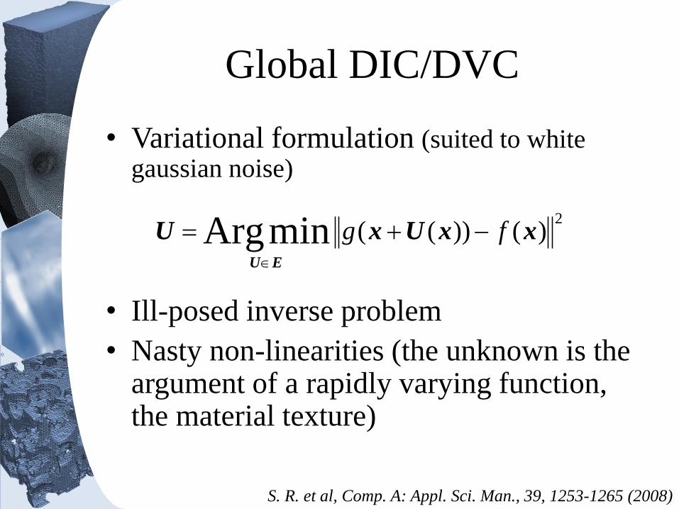
Global DIC/DVC
• Variational formulation (suited to white gaussian noise)
• Ill-posed inverse problem
• Nasty non-linearities (the unknown is the argument of a rapidly varying function, the material texture)
2)())((minArg xxUxU
EU
fg
S. R. et al, Comp. A: Appl. Sci. Man., 39, 1253-1265 (2008)
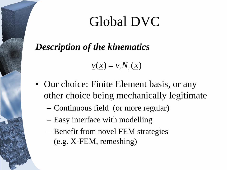
Global DVC
Description of the kinematics
• Our choice: Finite Element basis, or any
other choice being mechanically legitimate
– Continuous field (or more regular)
– Easy interface with modelling
– Benefit from novel FEM strategies
(e.g. X-FEM, remeshing)
)()( xNvxv ii
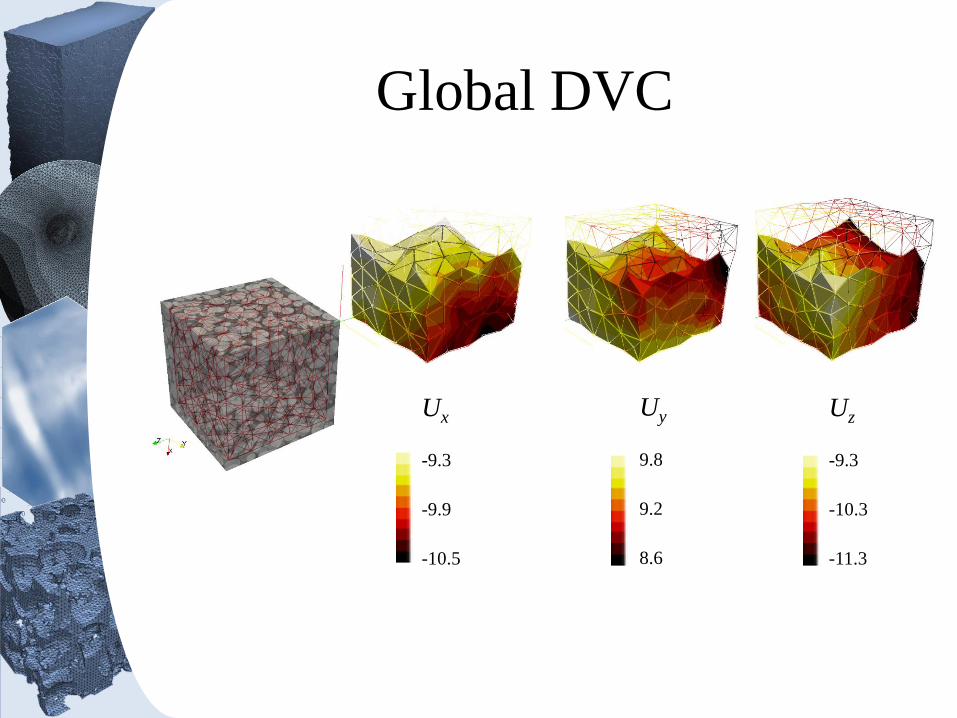
Global DVC
Ux
-9.3
-9.9
-10.5
Uy
9.8
9.2
8.6
Uz
-9.3
-10.3
-11.3
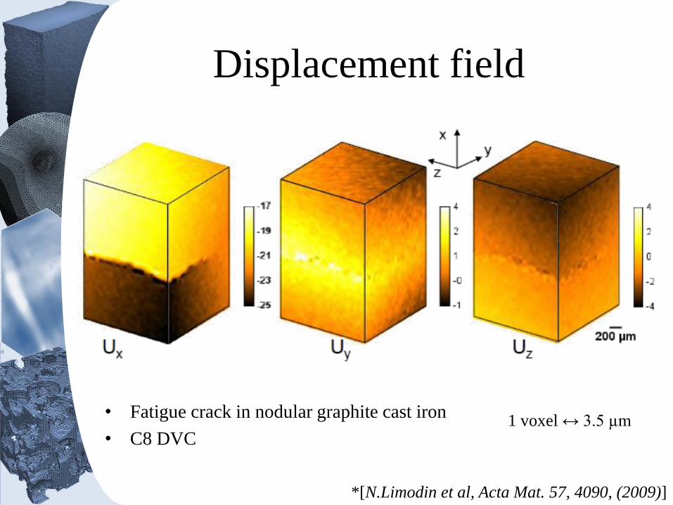
Displacement field
• Fatigue crack in nodular graphite cast iron
• C8 DVC 1 voxel ↔ 3.5 µm
*[N.Limodin et al, Acta Mat. 57, 4090, (2009)]
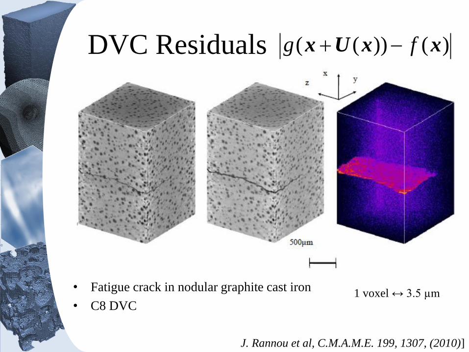
DVC Residuals
• Fatigue crack in nodular graphite cast iron
• C8 DVC 1 voxel ↔ 3.5 µm
J. Rannou et al, C.M.A.M.E. 199, 1307, (2010)]
)())(( xxUx fg
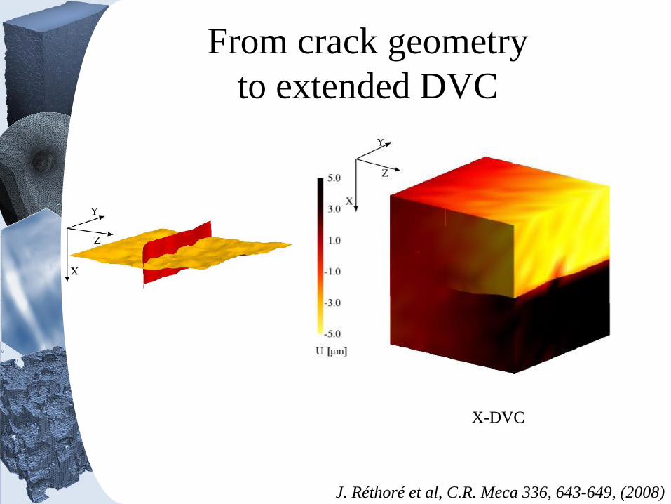
From crack geometry
to extended DVC
X-DVC
J. Réthoré et al, C.R. Meca 336, 643-649, (2008)
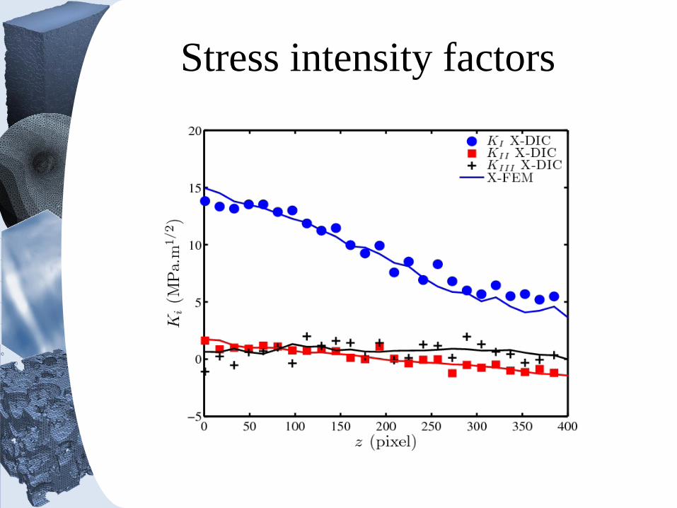
Stress intensity factors
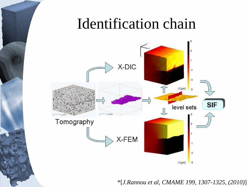
Identification chain
*[J.Rannou et al, CMAME 199, 1307-1325, (2010)]

Perspectives 2
DVC and extensions
• Adaptative multiscale DVC
• Noise management
• Residual-based re-meshing
• Exploitation of “topological differences’’
for segmenting, measuring, identifying,
detecting, …
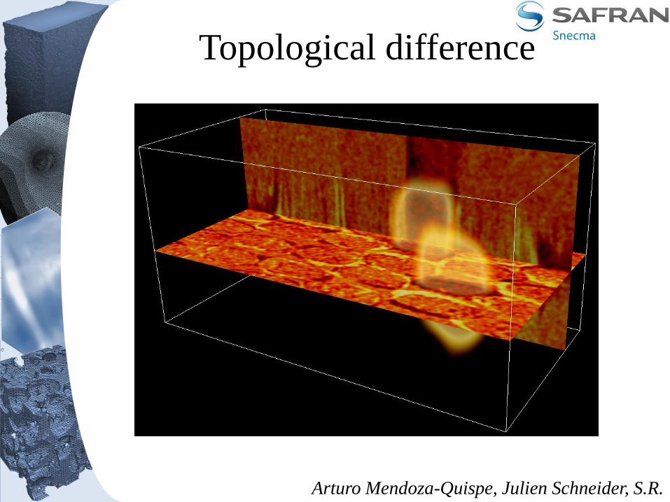
Arturo Mendoza-Quispe, Julien Schneider, S.R.
Topological difference
BEYOND THE LIMITS
New frontiers
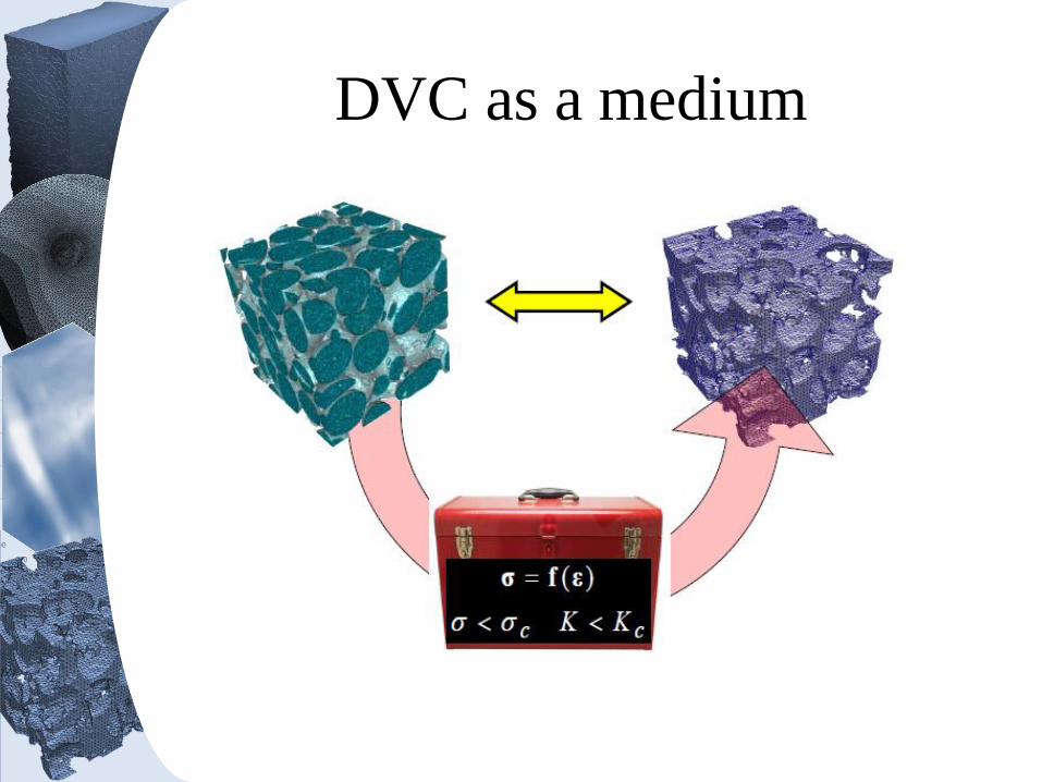
DVC as a medium
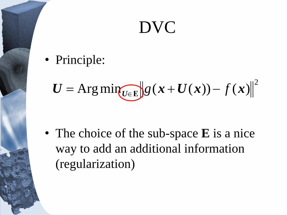
DVC
• Principle:
• The choice of the sub-space E is a nice
way to add an additional information
(regularization)
2)())((minArg xxUxU U fg Ε
Two routes for regularization
• Strong regularization:
– E is designed to have the smallest possible
dimensionality
– A small uncertainty is expected
– It is however delicate to picture the most
appropriate space E (not generic)
– “Haute couture”
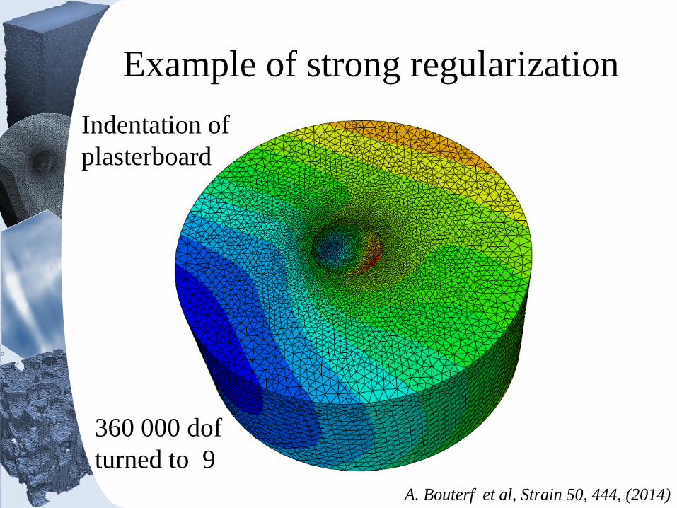
Example of strong regularization
A. Bouterf et al, Strain 50, 444, (2014)
Indentation of
plasterboard
360 000 dof
turned to 9
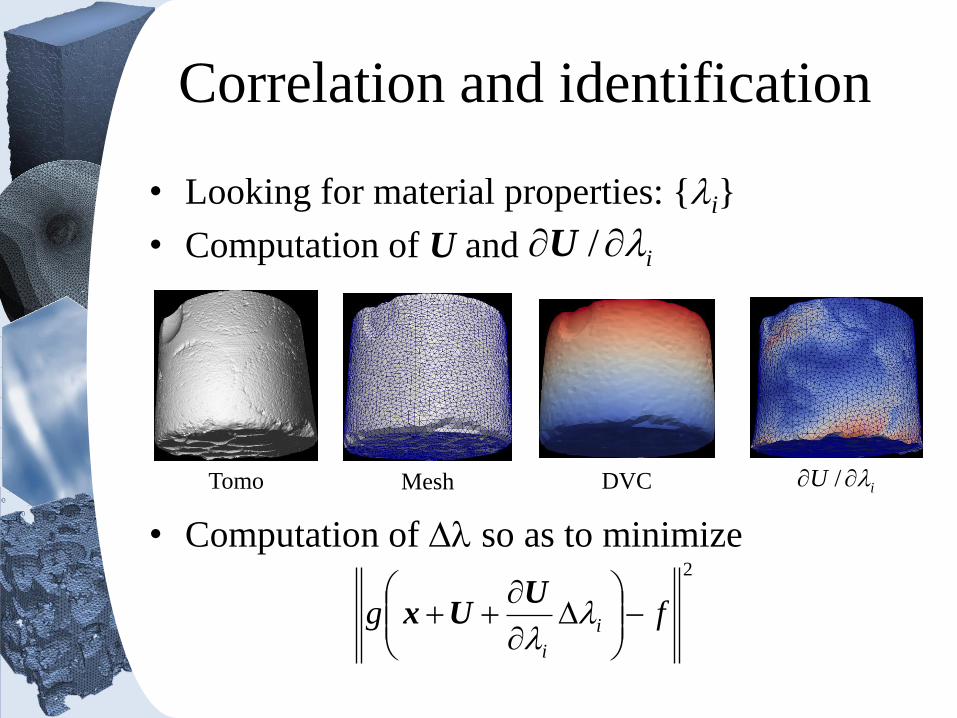
Correlation and identification
• Looking for material properties: {li}
• Computation of U and
• Computation of Dl so as to minimize
il /U
Tomo Mesh DVC iU l /
2
fg i
i
D
l
l
UUx
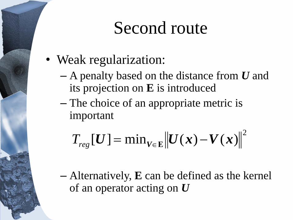
• Weak regularization:
– A penalty based on the distance from U and its projection on E is introduced
– The choice of an appropriate metric is important
– Alternatively, E can be defined as the kernel of an operator acting on U
Second route
2)()(min][ xVxUU V ΕregT
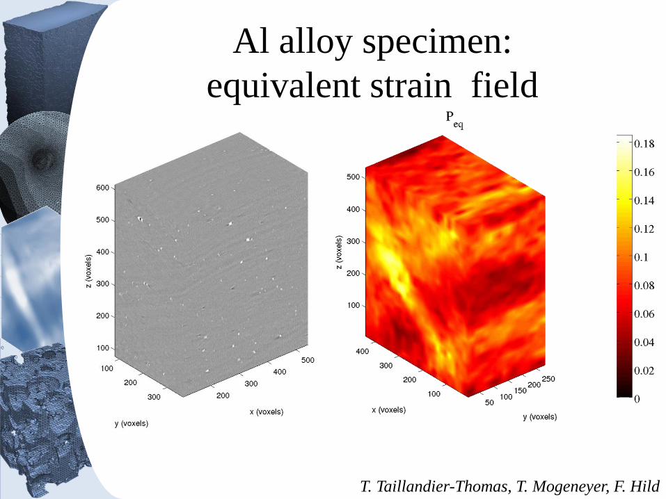
Al alloy specimen:
equivalent strain field
T. Taillandier-Thomas, T. Mogeneyer, F. Hild
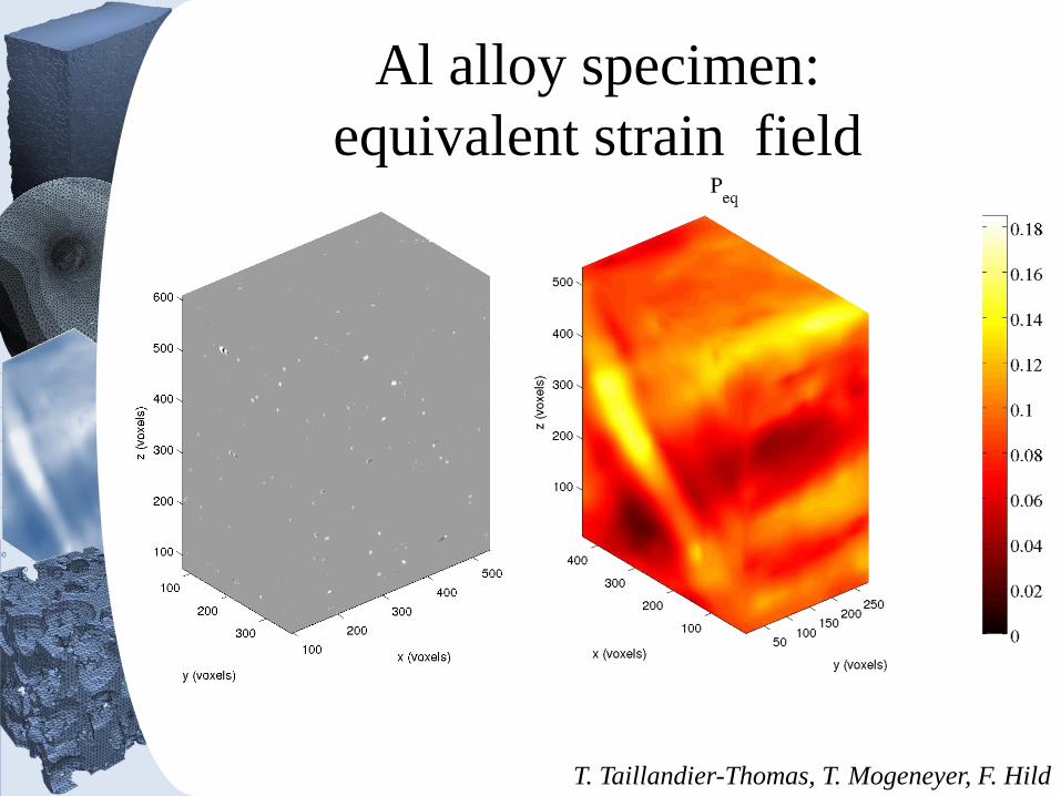
Al alloy specimen:
equivalent strain field
T. Taillandier-Thomas, T. Mogeneyer, F. Hild
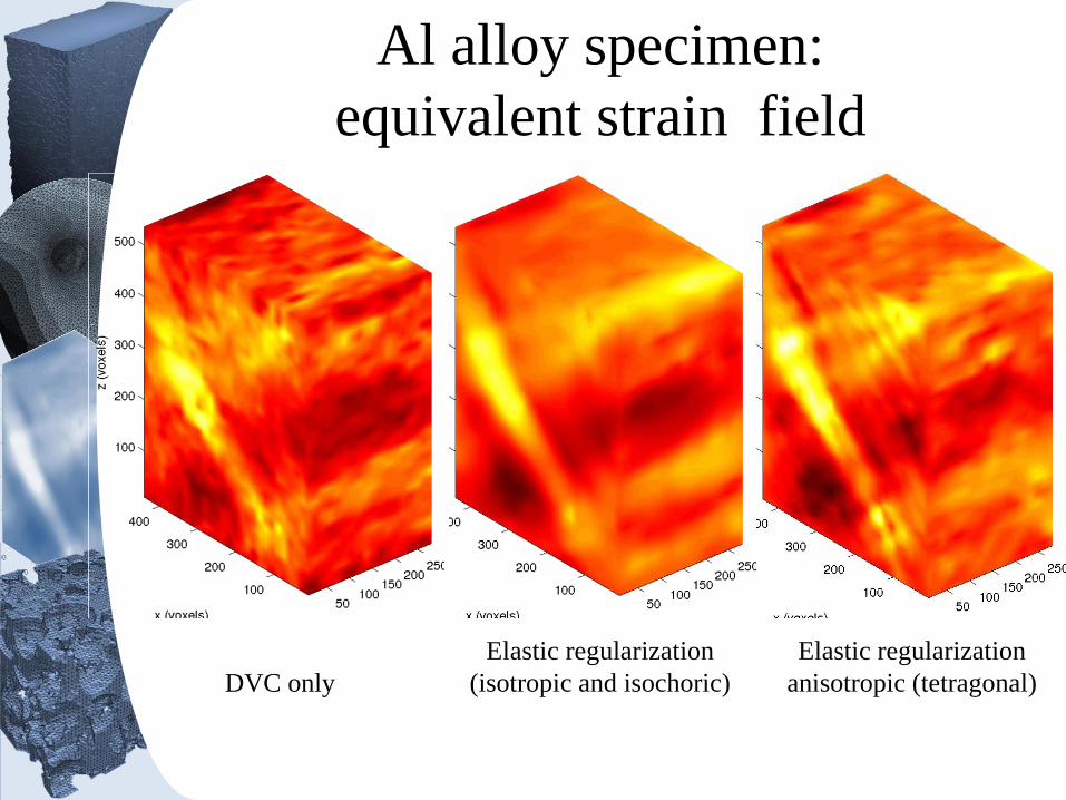
DVC only
Elastic regularization
(isotropic and isochoric)
Elastic regularization
anisotropic (tetragonal)
Al alloy specimen:
equivalent strain field

Perspectives 3
• New test design
• Multiphase identification
• Identification of complex constitutive
laws
• Efficient computation
4D
One additional challenge?
DVC without reconstruction
• Another approach to DVC
• Can the number of projections be
reduced?
• Kinematic complexity is much less than
that of the microstructure
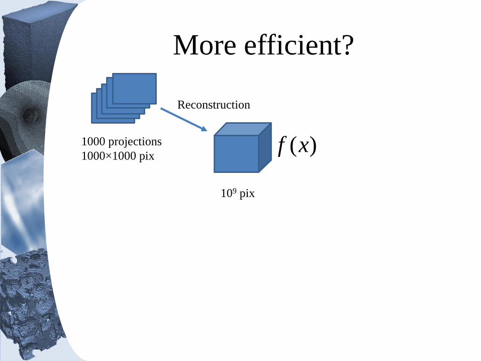
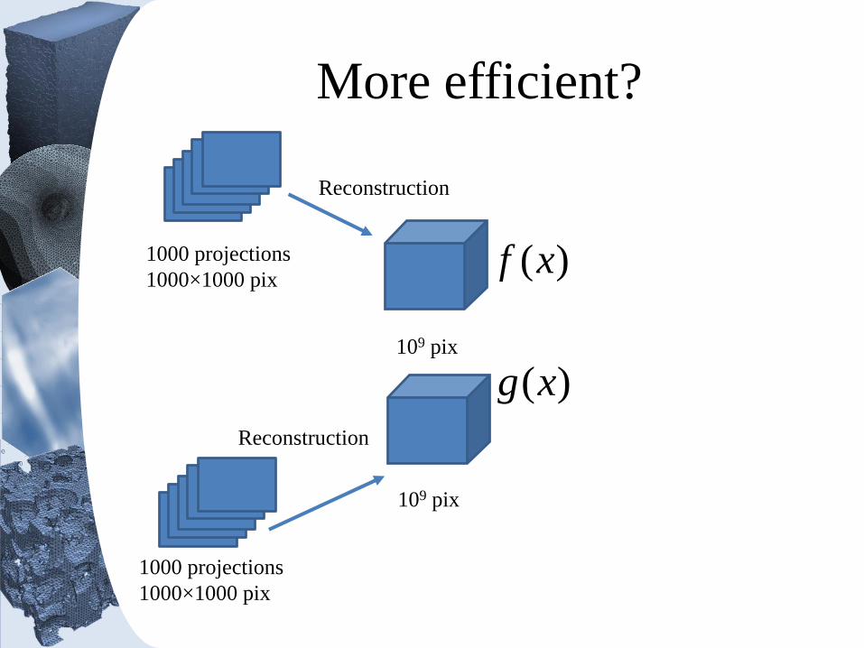
More efficient?
Reconstruction
1000 projections
1000×1000 pix
109 pix
)(xf
More efficient?
Reconstruction
1000 projections
1000×1000 pix
109 pix
Reconstruction
1000 projections
1000×1000 pix
109 pix
)(xf
)(xg
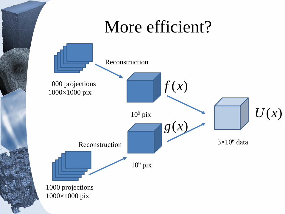
More efficient?
Reconstruction
1000 projections
1000×1000 pix
109 pix
3×106 data
)(xf
)(xg)(xU
Reconstruction
1000 projections
1000×1000 pix
109 pix
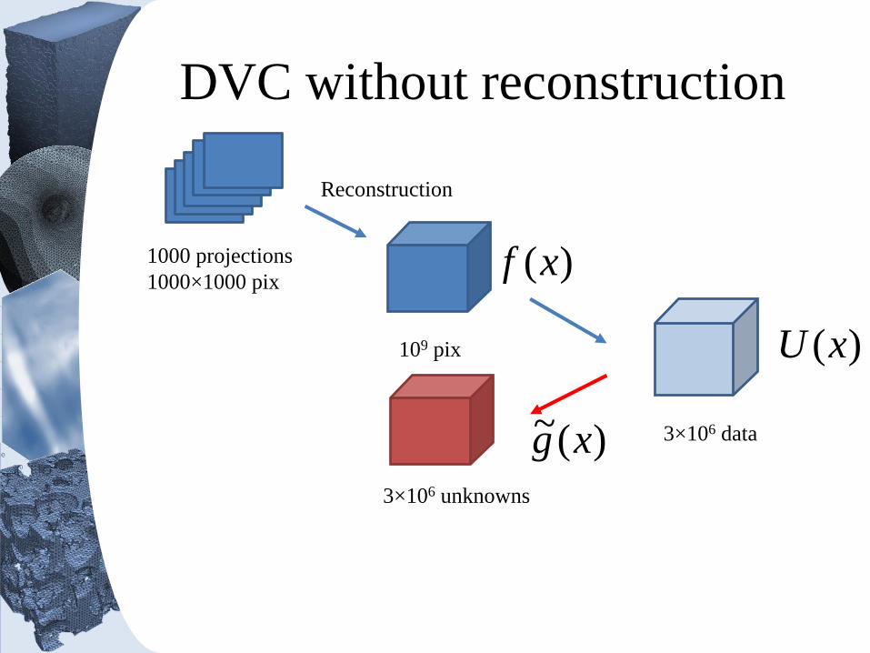
DVC without reconstruction
Reconstruction
1000 projections
1000×1000 pix
109 pix
3×106 data
)(xf
)(~ xg
)(xU
3×10⁶ unknowns
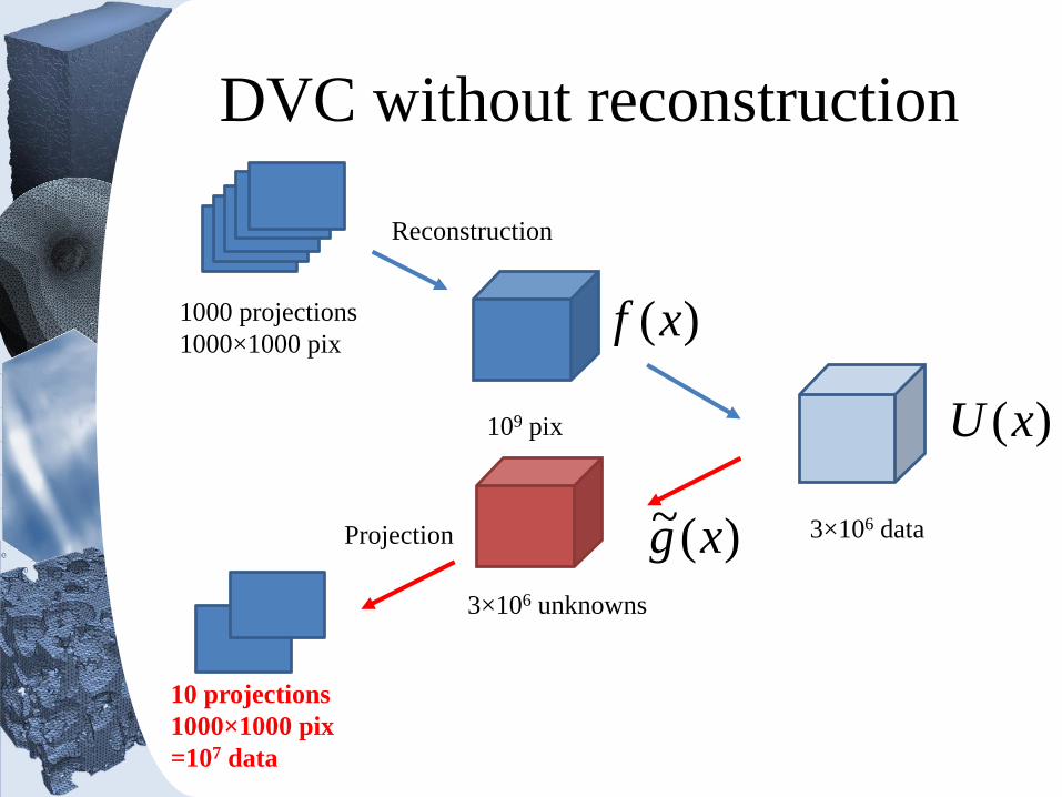
DVC without reconstruction
Reconstruction
1000 projections
1000×1000 pix
109 pix
3×106 data
)(xf
)(~ xg
)(xU
Projection
10 projections
1000×1000 pix
=107 data
3×10⁶ unknowns
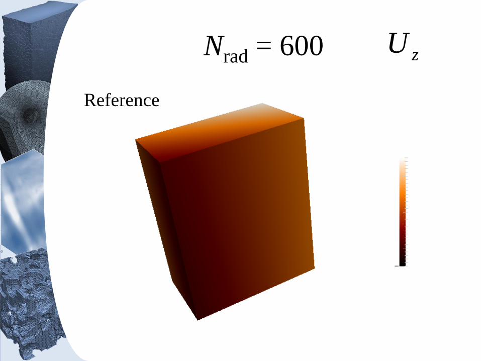
Nrad = 600 zU
Reference

Nrad = 48 zU

Nrad = 24 zU

Nrad = 12 zU
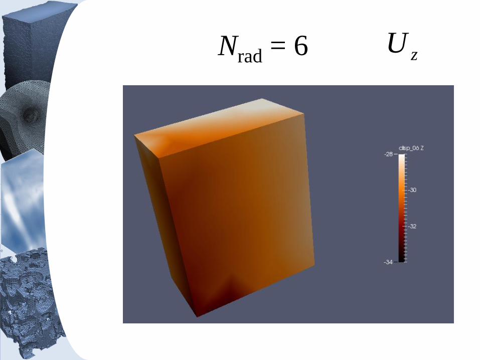
Nrad = 6 zU

Nrad = 3 zU

Nrad = 2 zU
DVC without reconstruction
• Gain in acquisition time = 99.7 % !
• Above 300-fold gain in saving.
• Temporal resolution can be increased by
a factor of 300!
• Can be combined with multiscale and
elastic regularization.
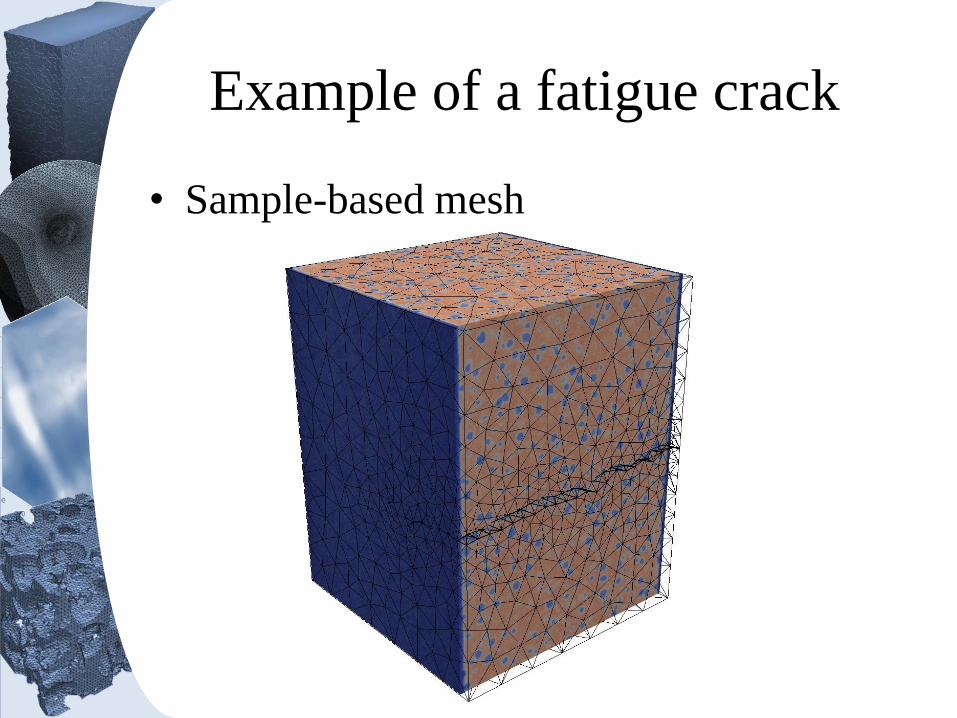
Example of a fatigue crack
• Sample-based mesh
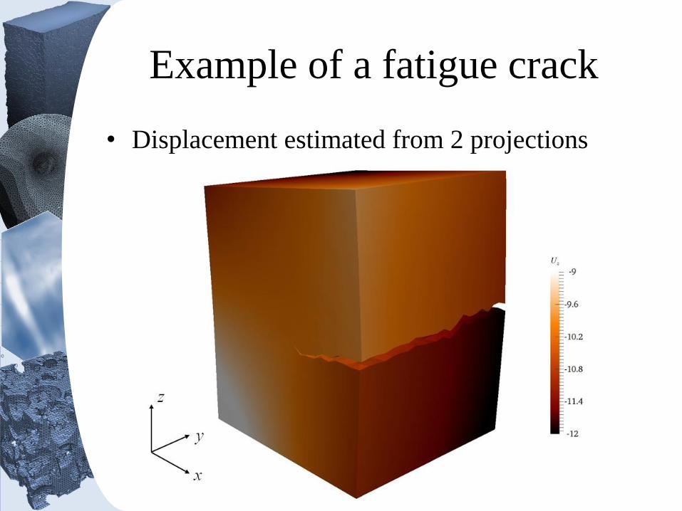
Example of a fatigue crack
• Displacement estimated from 2 projections
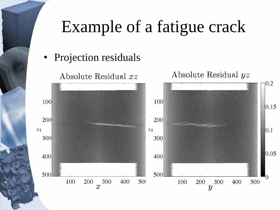
Example of a fatigue crack
• Projection residuals
DVC without reconstruction
Bonus:
• A proper handling of noise now becomes
easily feasible

Perspectives 4
• 4D Dynamic Tomography
• Cone-beam geometry is to be
implemented
• Adaptation to noise
• Application to identification
• More complex evolutions than motion
CONCLUSIONS

PERSPECTIVES
CONCLUSIONS
Perspectives
• Tomography allows for the analysis of
materials in their mechanical expression (in situ tests / reconstruction / DVC / identification)
• Coupling different treatments increases
robustness and provide data-sober solutions
• Considerable savings can be achieved
• Today tomography is fantastic, and
tomorrow will be even more so!

Tomographic « distillation »
Big data
Key data
Image mechanical properties
Image materials
Image motion
Image small defects
Image large defects
Experimental solid mechanics:
Towards the fourth dimension!
MATMECA Seminar, ONERA, Feb. 2016
Eikology team
Perspectives 1
• “Educated” tomographic reconstruction
• Exploitation of non voxel images (e.g. CAD based, reference based, or having a sparse parametrization)
• Instrument development: Phase contrast, or Diffraction contrast
Perspectives 2
DVC and extensions
• Adaptative multiscale DVC
• Noise management
• Residual-based re-meshing
• Exploitation of “topological differences’’
for segmenting, measuring, identifying,
detecting, …
Perspectives 3
• New test design
• Multiphase identification
• Identification of complex constitutive
laws
• Efficient computation
Perspectives 4
• 4D Dynamic Tomography
• Cone-beam geometry is to be
implemented
• Adaptation to noise
• Application to identification
• More complex evolutions than motion