www.iap.uni-jena.de

Imaging and Aberration Theory

Lecture 6: Spherical aberration

2012-11-23

Herbert Gross

Winter term 2012

2

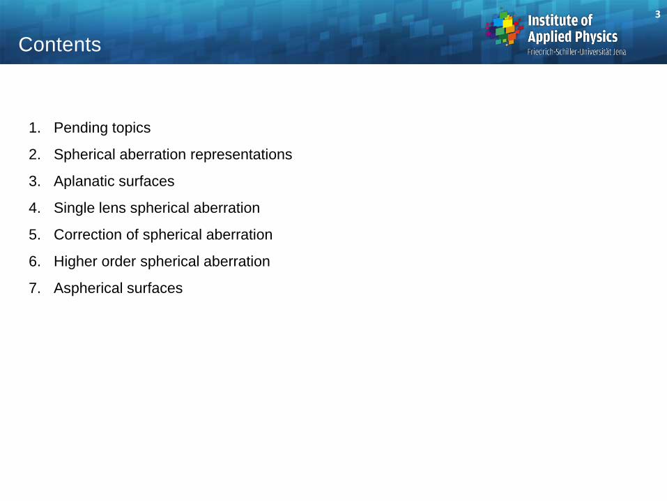
Preliminary time schedule

1 19.10. Paraxial imaging paraxial optics, fundamental laws of geometrical imaging, compound systems

2 26.10. Pupils, Fourier optics, Hamiltonian coordinates

pupil definition, basic Fourier relationship, phase space, analogy optics and mechanics, Hamiltonian coordinates

3 02.11. Eikonal Fermat Principle, stationary phase, Eikonals, relation rays-waves, geometrical approximation, inhomogeneous media

4 09.11. Aberration expansion single surface, general Taylor expansion, representations, various orders, stop shift formulas

5 16.11. Representations of aberrations different types of representations, fields of application, limitations and pitfalls, measurement of aberrations

6 23.11. Spherical aberration phenomenology, sph-free surfaces, skew spherical, correction of sph, aspherical surfaces, higher orders

7 07.12. Distortion and coma phenomenology, relation to sine condition, aplanatic sytems, effect of stop position, various topics, correction options

8 14.12. Astigmatism and curvature phenomenology, Coddington equations, Petzval law, correction options

9 21.12. Chromatical aberrations, Sine condition, isoplanasy

Dispersion, axial chromatical aberration, transverse chromatical aberration, sine condition, Herschel condition, isoplanays, relation to coma and shift invariance, pupil aberrations, relation to Fourier optics and phase space

10 11.01. Surface contributions sensitivity in 3rd order, structure of a system, superposition and induced aberrations, analysis of optical systems, lens contributions

11 18.01. Wave aberrations definition, various expansion forms, propagation of wave aberrations, relation to PSF and OTF

12 25.01. Zernike polynomials special expansion for circular symmetry, problems, calculation, optimal balancing, influence of normalization, recalculation for offset, ellipticity, measurement

13 01.02. Miscellaneous Aldi theorem, telecentric case, afocal case, aberration balancing, Delano diagram, Scheimpflug imaging, Fresnel lenses, statistical aberrations

14 08.02. Vectorial aberrations Introduction, special cases, actual research, anamorphotic, partial symmetric

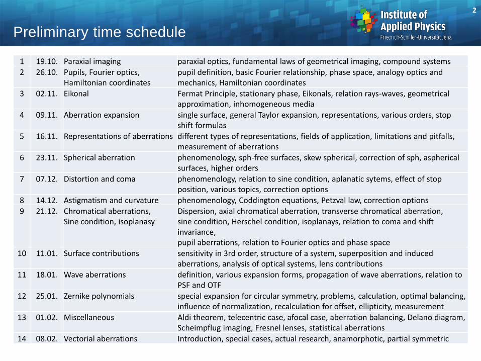
1. Pending topics

2. Spherical aberration representations

3. Aplanatic surfaces

4. Single lens spherical aberration

5. Correction of spherical aberration

6. Higher order spherical aberration

7. Aspherical surfaces

3

Contents

Typical Variation of Wave Aberrations

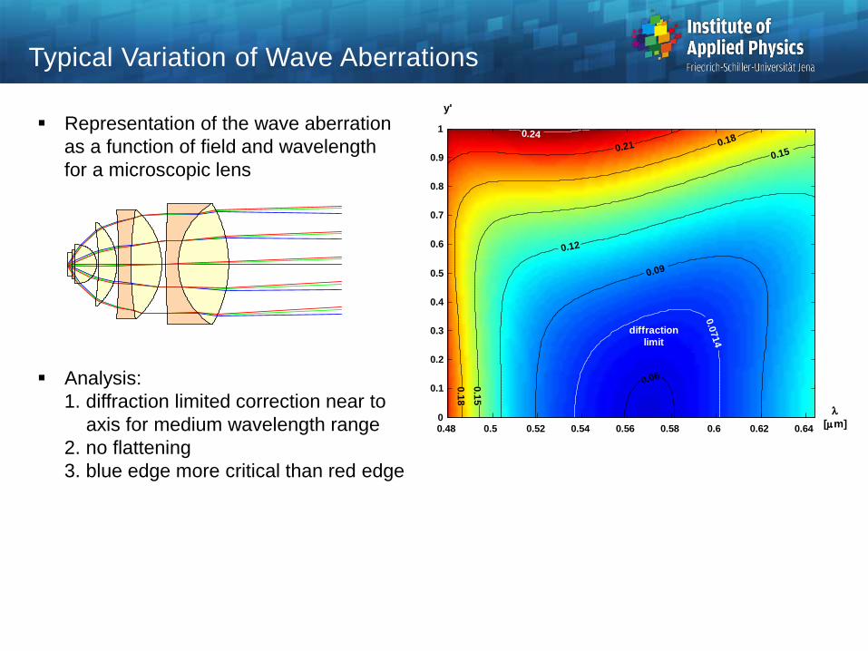
Representation of the wave aberration

as a function of field and wavelength

for a microscopic lens

Analysis:

1. diffraction limited correction near to

axis for medium wavelength range

2. no flattening

3. blue edge more critical than red edge

0.06

0.09

0.12

0.1

5

0.15

0.1

8

0.180.21

0.24

0.0

714

0

0.1

0.2

0.3

0.4

0.5

0.6

0.7

0.8

0.9

1

0.48 0.5 0.52 0.54 0.56 0.58 0.6 0.62 0.64

y'

[m]

diffraction

limit

Spatial Frequency of Wavefront Aberrations

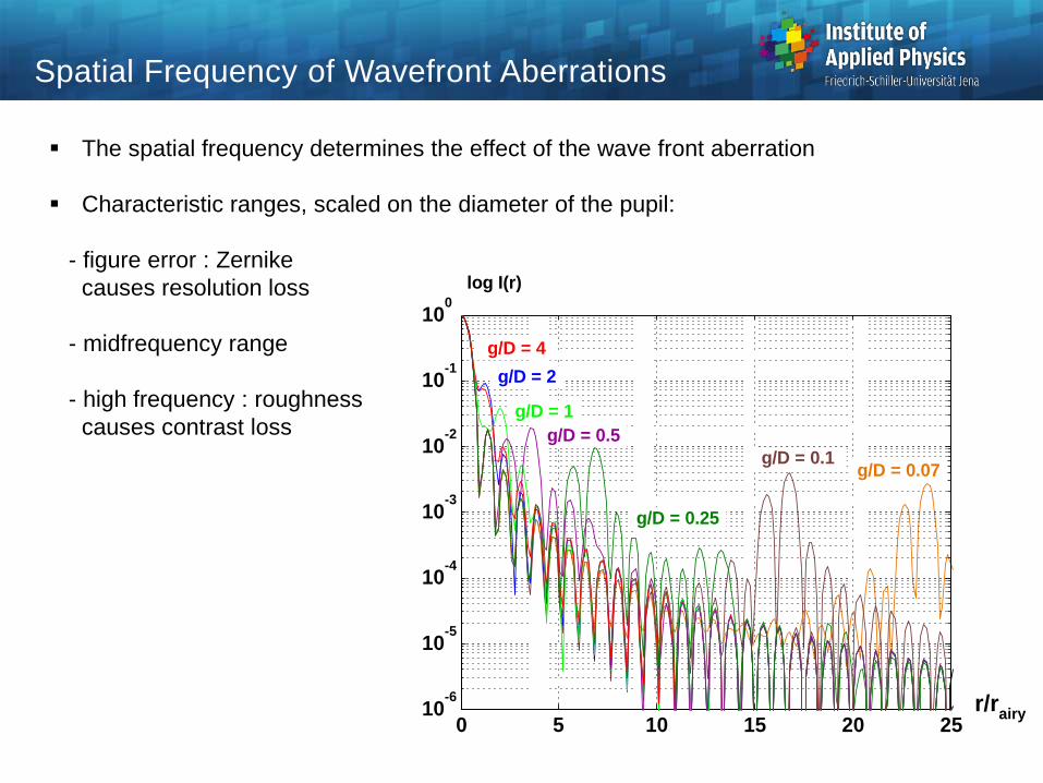
The spatial frequency determines the effect of the wave front aberration

Characteristic ranges, scaled on the diameter of the pupil:

- figure error : Zernike

causes resolution loss

- midfrequency range

- high frequency : roughness

causes contrast loss

log I(r)

0 5 10 15 20 2510

-6

10-5

10-4

10-3

10-2

10-1

100

r/rairy

g/D = 0.5

g/D = 4

g/D = 2

g/D = 1

g/D = 0.25

g/D = 0.07g/D = 0.1

Spatial Frequency of Surface Perturbations

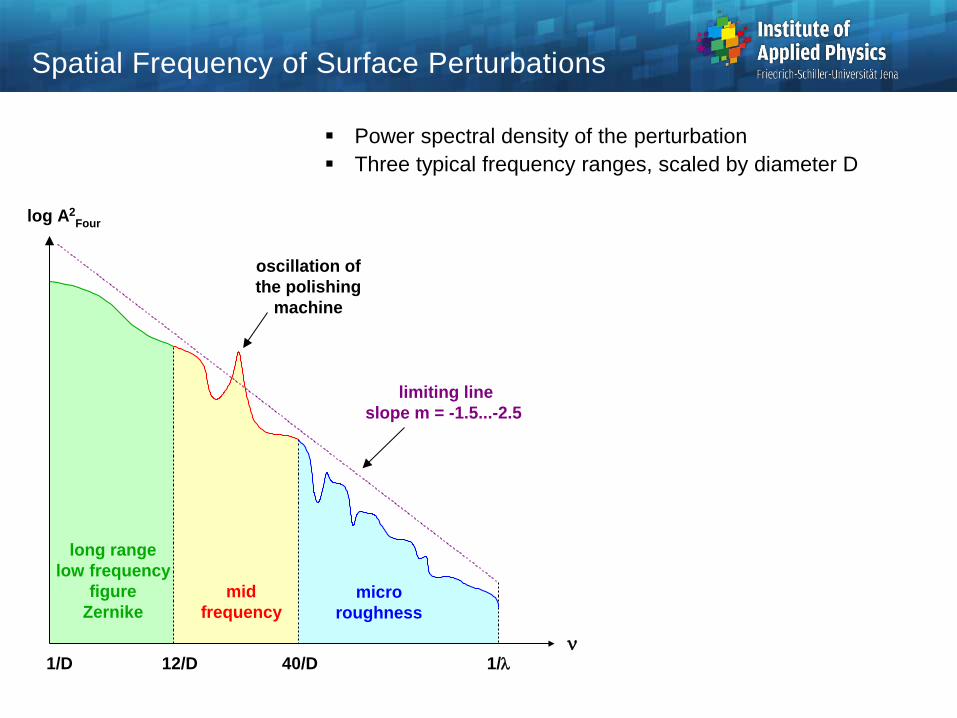
Power spectral density of the perturbation

Three typical frequency ranges, scaled by diameter D

limiting line

slope m = -1.5...-2.5

log A2Four

long range

low frequency

figure

Zernike

mid

frequencymicro

roughness

1/

oscillation of

the polishing

machine

12/D1/D 40/D

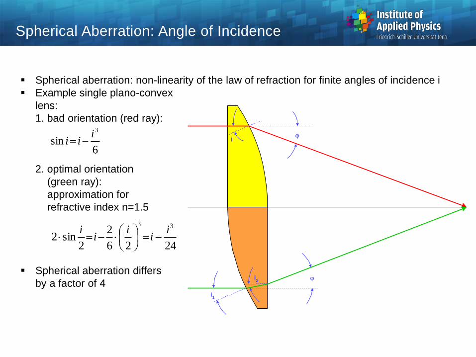
Spherical aberration: non-linearity of the law of refraction for finite angles of incidence i

Example single plano-convex

lens:

1. bad orientation (red ray):

2. optimal orientation

(green ray):

approximation for

refractive index n=1.5

Spherical aberration differs

by a factor of 4

ij

j

i1

i2

6sin

3iii

2426

2

2sin2

33i

ii

ii

Spherical Aberration: Angle of Incidence

Spherical Aberration

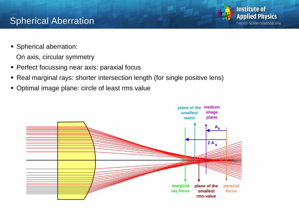
Spherical aberration:

On axis, circular symmetry

Perfect focussing near axis: paraxial focus

Real marginal rays: shorter intersection length (for single positive lens)

Optimal image plane: circle of least rms value

paraxial

focus

marginal

ray focusplane of the

smallest

rms-value

medium

image

plane

As

plane of the

smallest

waist

2 A s

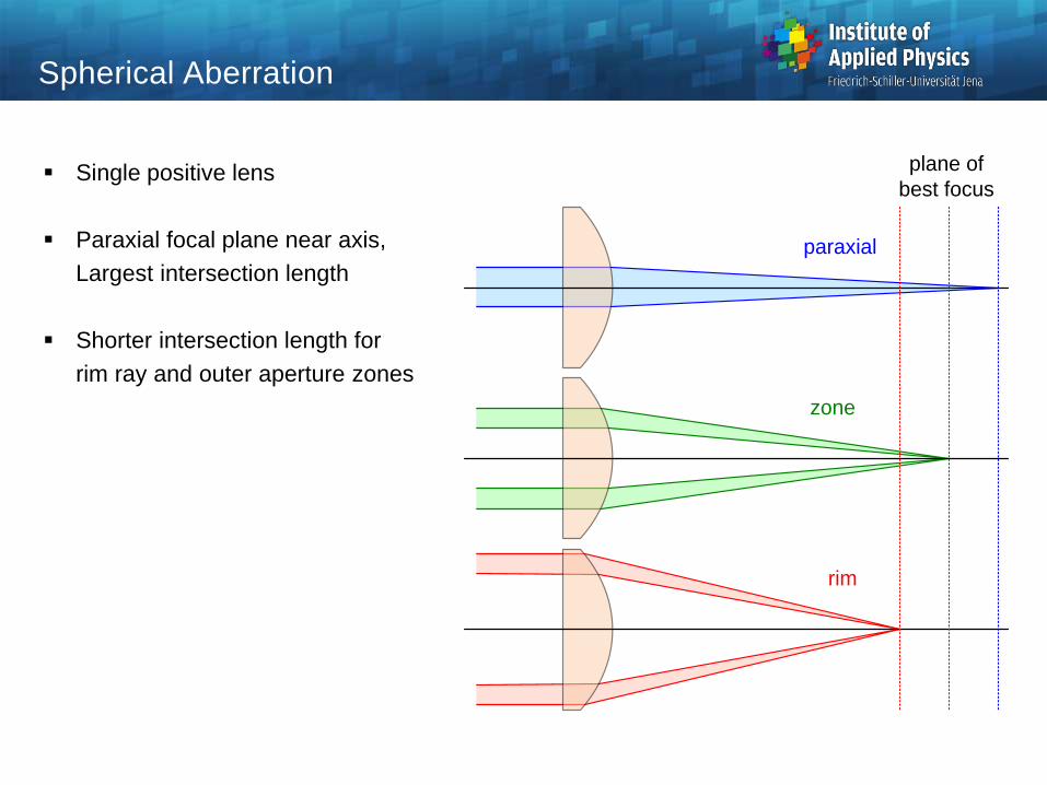
Spherical Aberration

Single positive lens

Paraxial focal plane near axis,

Largest intersection length

Shorter intersection length for

rim ray and outer aperture zones

plane of

best focus

zone

paraxial

rim

rp

+1

-1

+1

A / A = -1.33sd

A / A = -1.0sd

A / A = -1.5sd

A / A = -2.0sd

A / A = 0.0sd

A sW /

42

pspd rArAW

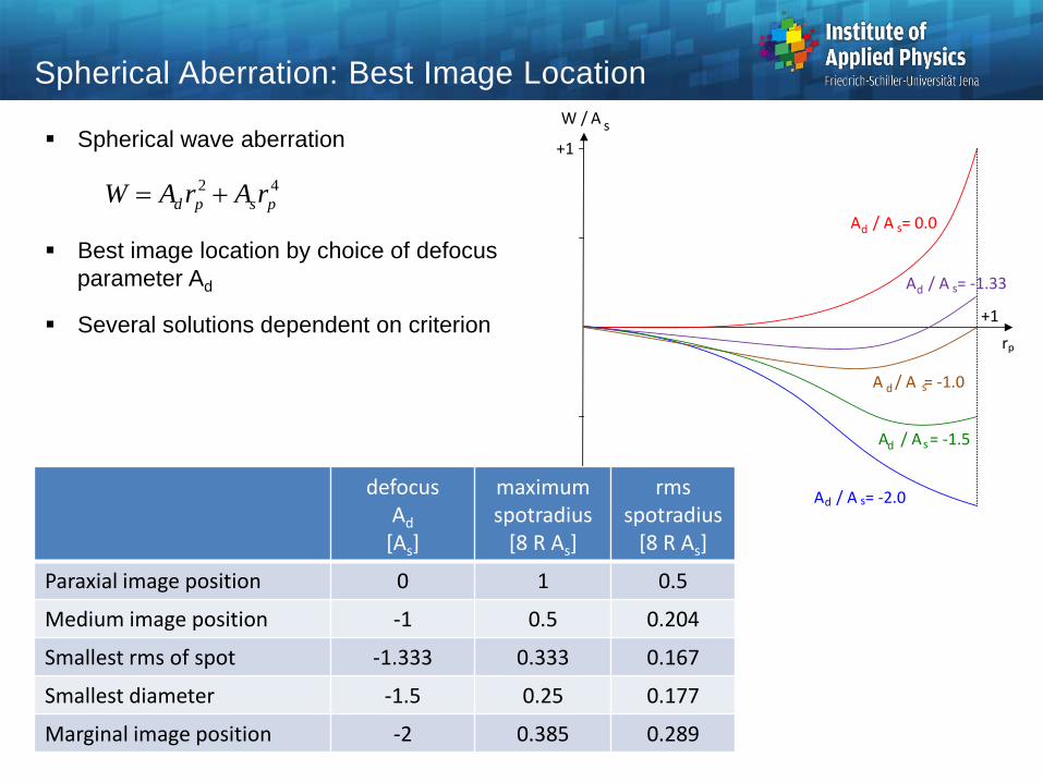
Spherical Aberration: Best Image Location

Spherical wave aberration

Best image location by choice of defocus

parameter Ad

Several solutions dependent on criterion

defocus Ad

[As]

maximum spotradius

[8 R As]

rms spotradius

[8 R As]

Paraxial image position 0 1 0.5

Medium image position -1 0.5 0.204

Smallest rms of spot -1.333 0.333 0.167

Smallest diameter -1.5 0.25 0.177

Marginal image position -2 0.385 0.289

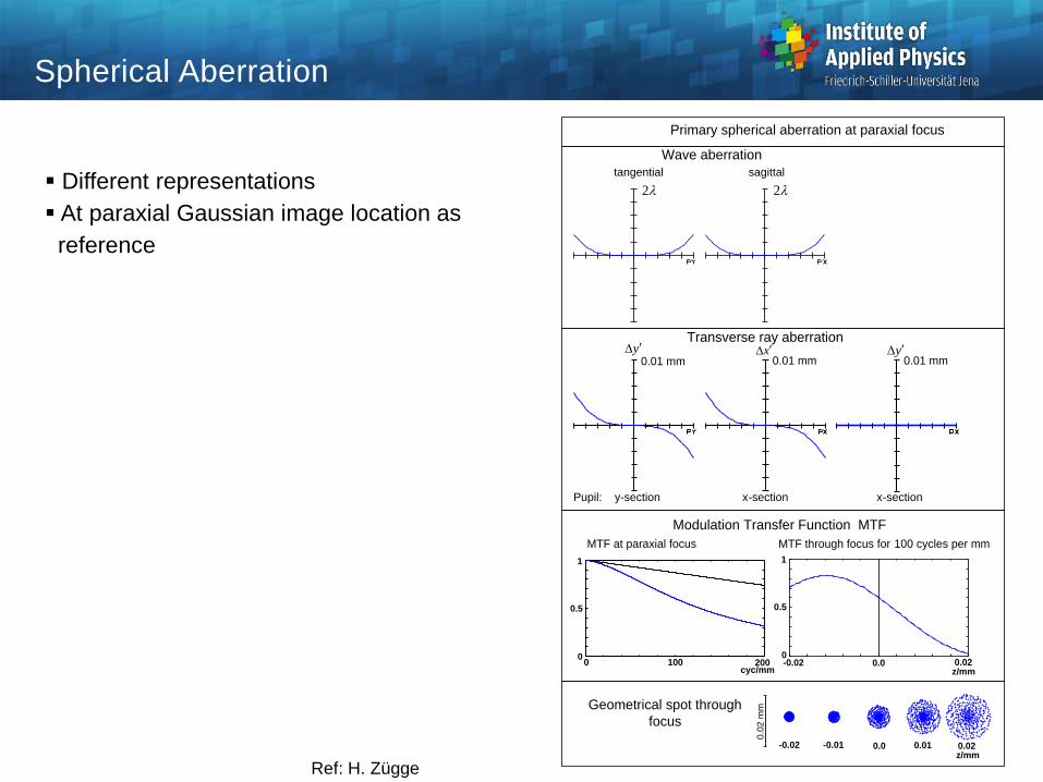
Spherical Aberration

Wave aberration

tangential sagittal

22

Primary spherical aberration at paraxial focus

Transverse ray aberration y x y

Pupil: y-section x-section x-section

0.01 mm 0.01 mm 0.01 mm

Geometrical spot through

focus

0.0

2 m

m

Modulation Transfer Function MTF

MTF at paraxial focus MTF through focus for 100 cycles per mm

1

0

0.5

0 100 200cyc/mm z/mm

1

0

0.5

-0.02 0.020.0

z/mm-0.02 0.020.0-0.01 0.01

Ref: H. Zügge

Different representations

At paraxial Gaussian image location as

reference

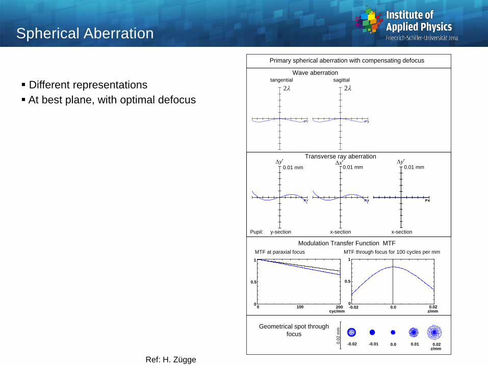
Different representations

At best plane, with optimal defocus

Spherical Aberration

Wave aberrationtangential sagittal

22

Primary spherical aberration with compensating defocus

y x y

Pupil: y-section x-section x-section

0.01 mm 0.01 mm 0.01 mm

Transverse ray aberration

Geometrical spot through

focus0.0

2 m

m

Modulation Transfer Function MTF

MTF at paraxial focus MTF through focus for 100 cycles per mm

z/mm-0.02 0.020.0-0.01 0.01

1

0

0.5

0 100 200cyc/mm z/mm

1

0

0.5

0.020.0-0.02

Ref: H. Zügge

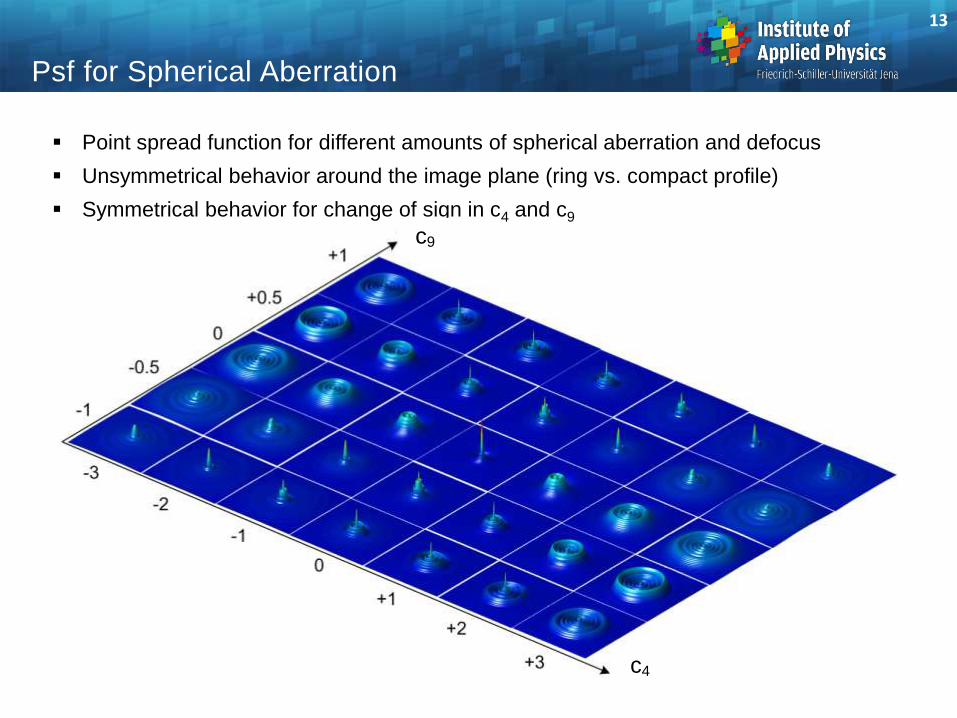
Psf for Spherical Aberration

Point spread function for different amounts of spherical aberration and defocus

Unsymmetrical behavior around the image plane (ring vs. compact profile)

Symmetrical behavior for change of sign in c4 and c9

13

c9

c4

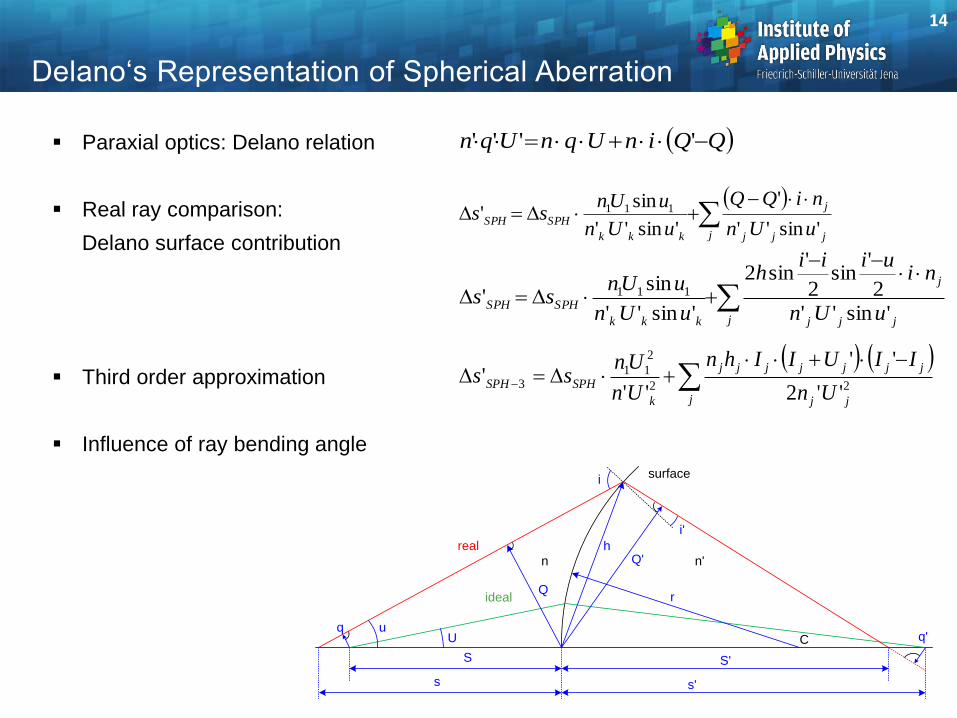
Delano‘s Representation of Spherical Aberration

Paraxial optics: Delano relation

Real ray comparison:

Delano surface contribution

Third order approximation

Influence of ray bending angle

14

real

ideal

uU

i

i'

Q

Q'

s

S

s'

S'

surface

n'n

q

h

q'C

r

QQinUqnUqn ''''

j jj

jjjjjjj

k

SPHSPHUn

IIUIIhn

Un

Unss

22

2

113

''2

''

'''

j jjj

j

kkk

SPHSPHuUn

niQQ

uUn

uUnss

'sin''

'

'sin''

sin' 111

j jjj

j

kkk

SPHSPHuUn

niuiii

h

uUn

uUnss

'sin''2

'sin

2

'sin2

'sin''

sin' 111

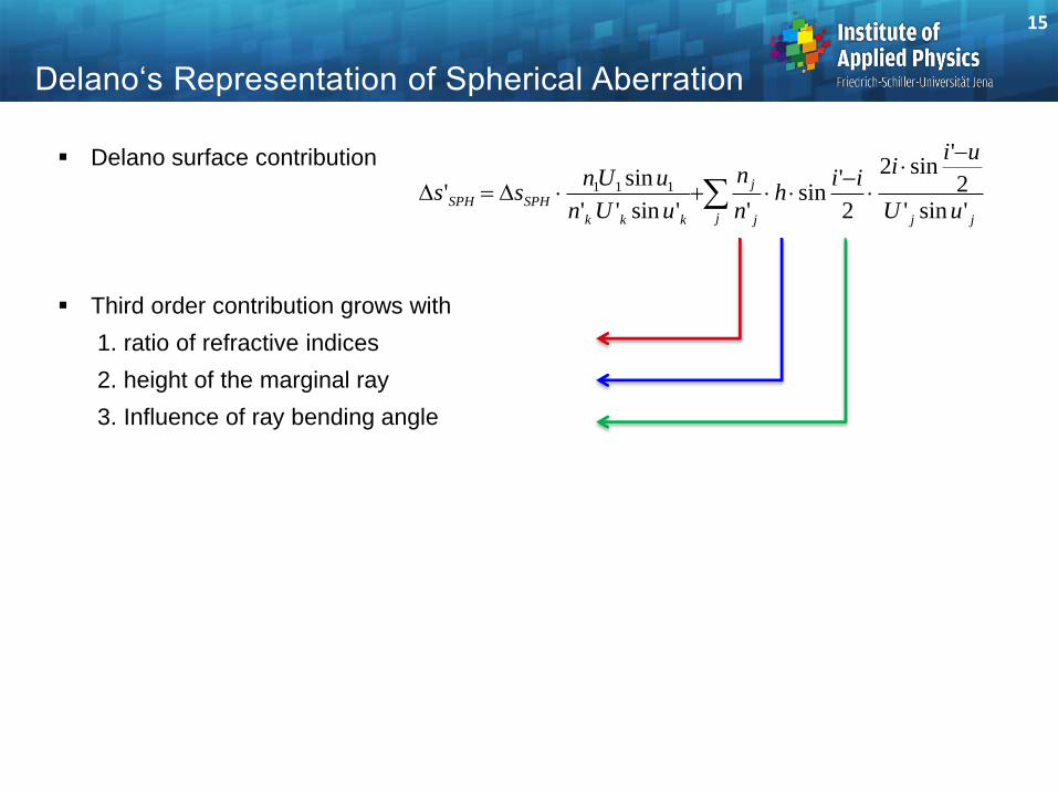
Delano‘s Representation of Spherical Aberration

Delano surface contribution

Third order contribution grows with

1. ratio of refractive indices

2. height of the marginal ray

3. Influence of ray bending angle

15

j jjj

j

kkk

SPHSPHuU

uii

iih

n

n

uUn

uUnss

'sin'2

'sin2

2

'sin

''sin''

sin' 111

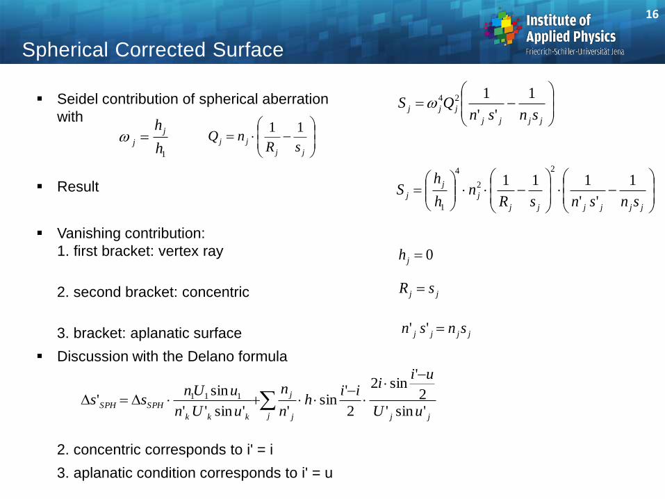
Spherical Corrected Surface

Seidel contribution of spherical aberration

with

Result

Vanishing contribution:

1. first bracket: vertex ray

2. second bracket: concentric

3. bracket: aplanatic surface

Discussion with the Delano formula

2. concentric corresponds to i' = i

3. aplanatic condition corresponds to i' = u

16

jjjj

jjjsnsn

QS1

''

124

j

jh

h

1

jj

jjsR

nQ11

jjjjjj

j

j

jsnsnsR

nh

hS

1

''

1112

2

4

1

0jh

jjjj snsn ''

jj sR

j jjj

j

kkk

SPHSPHuU

uii

iih

n

n

uUn

uUnss

'sin'2

'sin2

2

'sin

''sin''

sin' 111

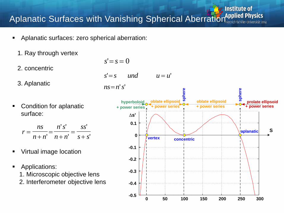
Aplanatic Surfaces with Vanishing Spherical Aberration

s'

0 50 100 150 200 250 300-0.5

-0.4

-0.3

-0.2

-0.1

0

0.1

Saplanatic

concentricvertex

oblate ellipsoidoblate ellipsoid prolate ellipsoidhyperboloid+ power series + power series+ power series + power series

sp

he

re

sp

he

re

Aplanatic surfaces: zero spherical aberration:

1. Ray through vertex

2. concentric

3. Aplanatic

Condition for aplanatic

surface:

Virtual image location

Applications:

1. Microscopic objective lens

2. Interferometer objective lens

s s und u u' '

s s' 0

ns n s ' '

rns

n n

n s

n n

ss

s s

'

' '

'

'

'

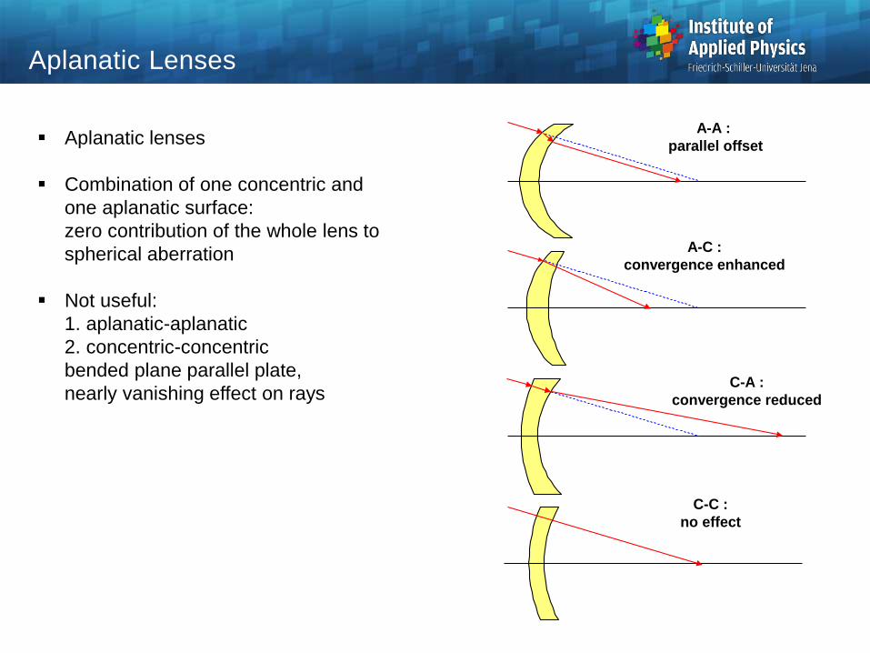
Aplanatic lenses

Combination of one concentric and

one aplanatic surface:

zero contribution of the whole lens to

spherical aberration

Not useful:

1. aplanatic-aplanatic

2. concentric-concentric

bended plane parallel plate,

nearly vanishing effect on rays

Aplanatic Lenses

A-A :

parallel offset

A-C :

convergence enhanced

C-C :

no effect

C-A :

convergence reduced

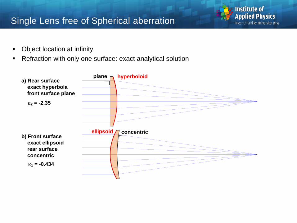
Single Lens free of Spherical aberration

Object location at infinity

Refraction with only one surface: exact analytical solution

planea) Rear surface

exact hyperbola

front surface plane

b) Front surface

exact ellipsoid

rear surface

concentric

k2 = -2.35

k1 = -0.434

concentric

hyperboloid

ellipsoid

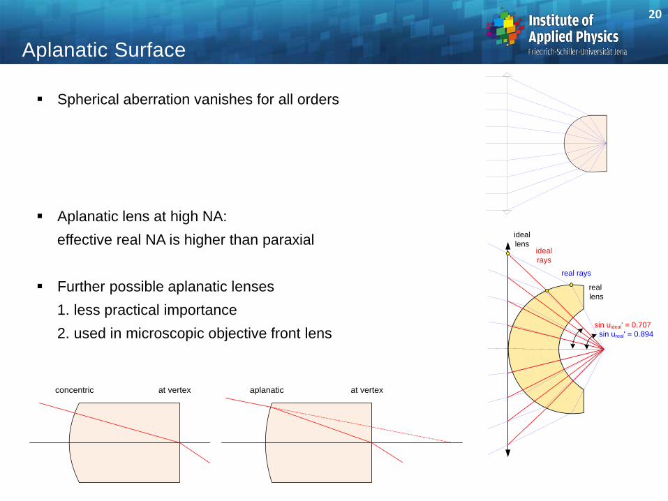
Aplanatic Surface

Spherical aberration vanishes for all orders

Aplanatic lens at high NA:

effective real NA is higher than paraxial

Further possible aplanatic lenses

1. less practical importance

2. used in microscopic objective front lens

20

concentric at vertex aplanatic at vertex

real rays

ideal

lensideal

rays

real

lens

sin ureal' = 0.894

sin uideal' = 0.707

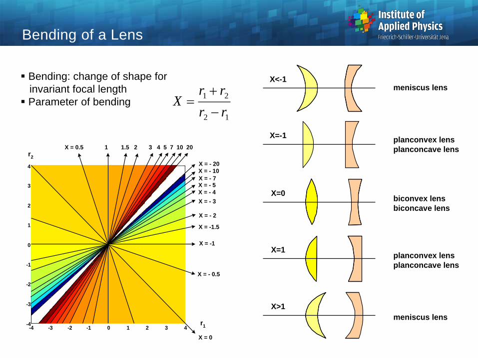
Bending of a Lens

Bending: change of shape for

invariant focal length

Parameter of bending

r1

r2

X = -1

X = 0.5 1 1.5 2 3 4 5 7 10 20

-4 -3 -2 -1 0 1 2 3 4-4

-3

-2

-1

0

1

2

3

4

X = -1.5

X = - 0.5

X = 0

X = - 2

X = - 3

X = - 4

X = - 5X = - 7

X = - 10

X = - 20

12

21

rr

rrX

X=1

X>1

X=0

X=-1

meniscus lensX<-1

biconvex lens

biconcave lens

planconvex lens

planconcave lens

planconvex lens

planconcave lens

meniscus lens

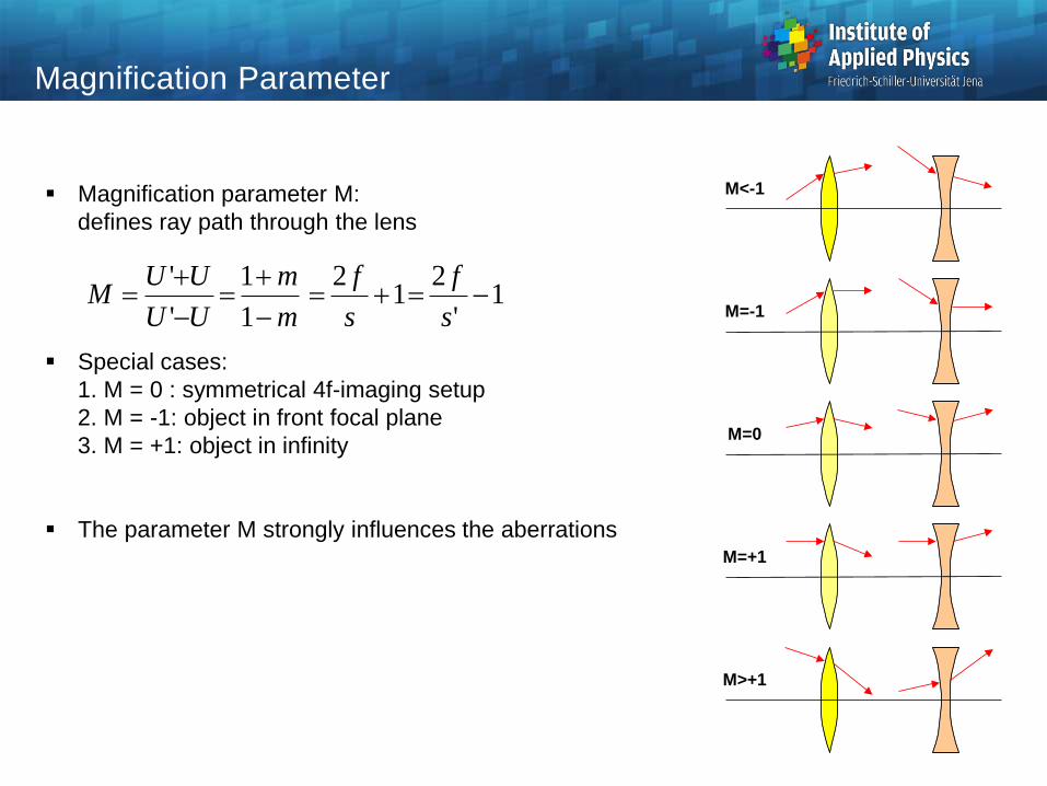
Magnification parameter M:

defines ray path through the lens

Special cases:

1. M = 0 : symmetrical 4f-imaging setup

2. M = -1: object in front focal plane

3. M = +1: object in infinity

The parameter M strongly influences the aberrations

1'

21

2

1

1

'

'

s

f

s

f

m

m

UU

UUM

Magnification Parameter

M=0

M=-1

M<-1

M=+1

M>+1

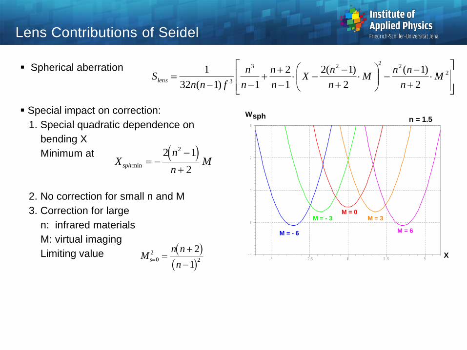
Lens Contributions of Seidel

Spherical aberration

Special impact on correction:

1. Special quadratic dependence on

bending X

Minimum at

2. No correction for small n and M

3. Correction for large

n: infrared materials

M: virtual imaging

Limiting value

2

22

23

3 2

)1(

2

)1(2

1

2

1)1(32

1M

n

nnM

n

nX

n

n

n

n

fnnSlens

sphW

X

M = 6M = - 6

M = - 3M = 0

M = 3

n = 1.5

X

n

nMsph min

2 1

2

2

M

n n

ns

0

2

2

2

1

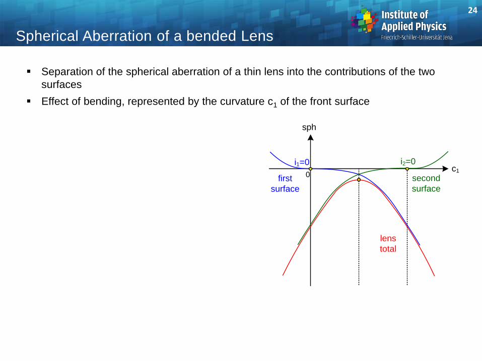
Spherical Aberration of a bended Lens

Separation of the spherical aberration of a thin lens into the contributions of the two

surfaces

Effect of bending, represented by the curvature c1 of the front surface

24

sph

c10

i1=0 i2=0

first

surface

second

surface

lens

total

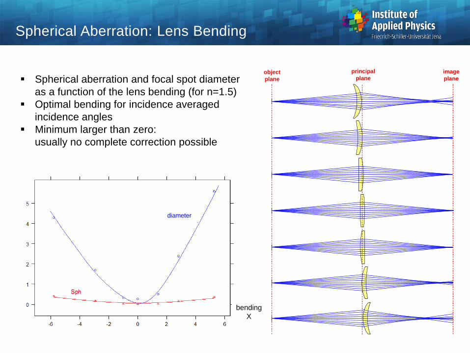
Spherical aberration and focal spot diameter

as a function of the lens bending (for n=1.5)

Optimal bending for incidence averaged

incidence angles

Minimum larger than zero:

usually no complete correction possible

Spherical Aberration: Lens Bending

object

plane

image

plane

principal

plane

diameter

bending

X

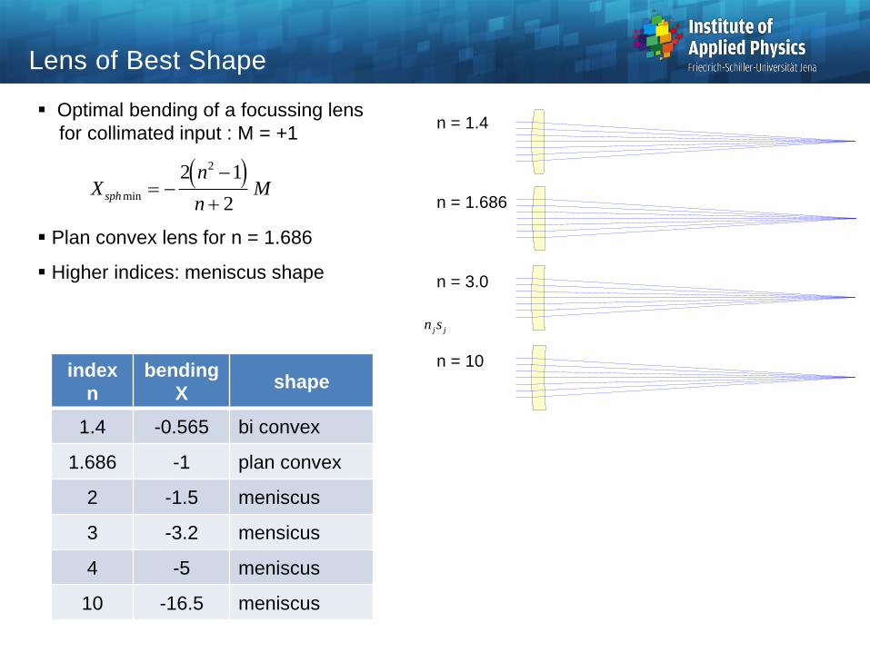
Lens of Best Shape

Optimal bending of a focussing lens

for collimated input : M = +1

Plan convex lens for n = 1.686

Higher indices: meniscus shape

X

n

nMsph min

2 1

2

2

n = 1.4

n = 1.686

n = 3.0

n = 10

jjsn

index

n

bending

X shape

1.4 -0.565 bi convex

1.686 -1 plan convex

2 -1.5 meniscus

3 -3.2 mensicus

4 -5 meniscus

10 -16.5 meniscus

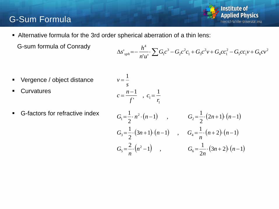
G-Sum Formula

Alternative formula for the 3rd order spherical aberration of a thin lens:

G-sum formula of Conrady

Vergence / object distance

Curvatures

G-factors for refractive index

2

615

2

14

2

31

2

2

3

1

4

''' cvGvccGccGvcGccGcG

un

hs sph

sv

1

1

1

1,

'

1

rc

f

nc

1232

1,1

2

121

,1132

1

1122

1,1

2

1

6

2

5

43

2

2

1

nnn

Gnn

G

nnn

GnnG

nnGnnG

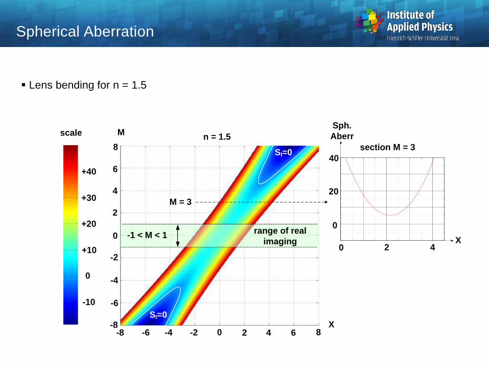
Lens bending for n = 1.5

Spherical Aberration

scale

-10

0

+10

+20

+30

+40

X

M

SI=0

n = 1.5

range of real

imaging

SI=0

0 2 4 6 8-2-4-6-8

0

2

4

6

8

-2

-4

-6

-8

section M = 3

0

42

40

0

20M = 3

Sph.

Aberr

X-1 < M < 1

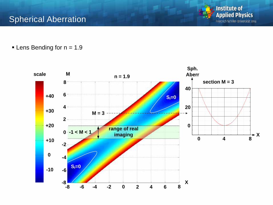
Lens Bending for n = 1.9

Spherical Aberration

scale

-10

0

+10

+20

+30

+40

X

M

SI=0

n = 1.9

range of real

imaging

SI=0

0 2 4 6 8-2-4-6-8

0

2

4

6

8

-2

-4

-6

-8

section M = 3

0

4 8

40

0

20

-1 < M < 1

Sph.

Aberr

X

M = 3

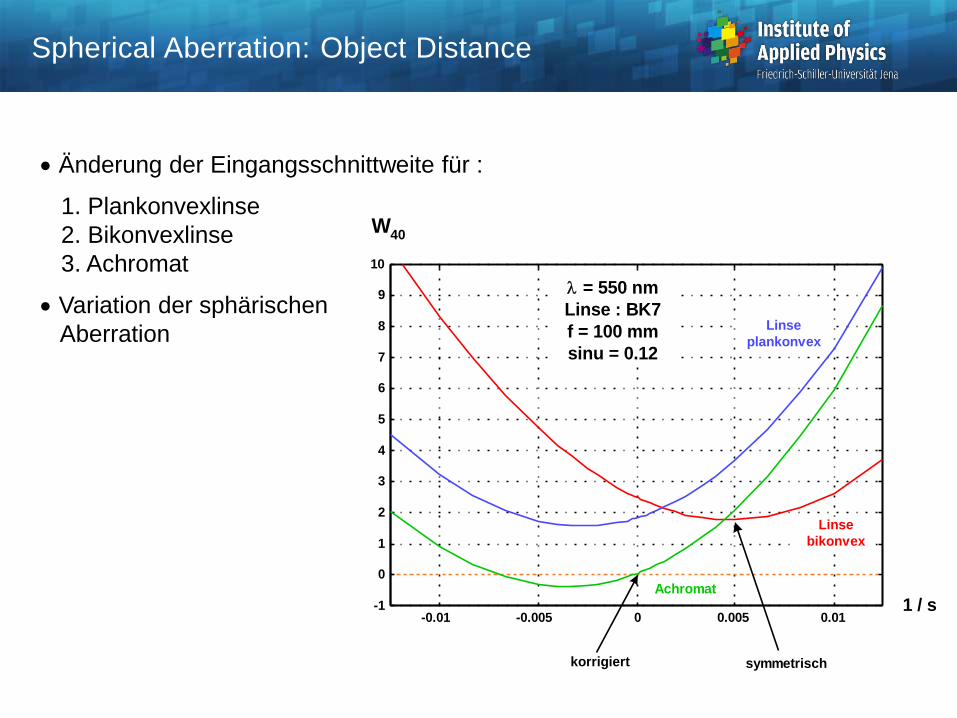
Änderung der Eingangsschnittweite für :

1. Plankonvexlinse

2. Bikonvexlinse

3. Achromat

Variation der sphärischen

Aberration

-0.01 -0.005 0 0.005 0.01-1

0

1

2

3

4

5

6

7

8

9

10

W40

1 / s

Linse

bikonvex

Linse

plankonvex

Achromat

= 550 nm

Linse : BK7

f = 100 mm

sinu = 0.12

symmetrischkorrigiert

Spherical Aberration: Object Distance

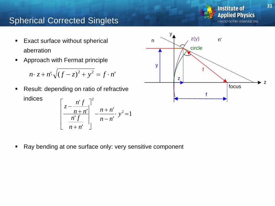
Spherical Corrected Singlets

Exact surface without spherical

aberration

Approach with Fermat principle

Result: depending on ratio of refractive

indices

Ray bending at one surface only: very sensitive component

31

focus

f

y

n

z

n'z(y)y

z

circle

f')(' 22 nfyzfnzn

1'

'

'

''

'

2

2

ynn

nn

nn

fnnn

fnz

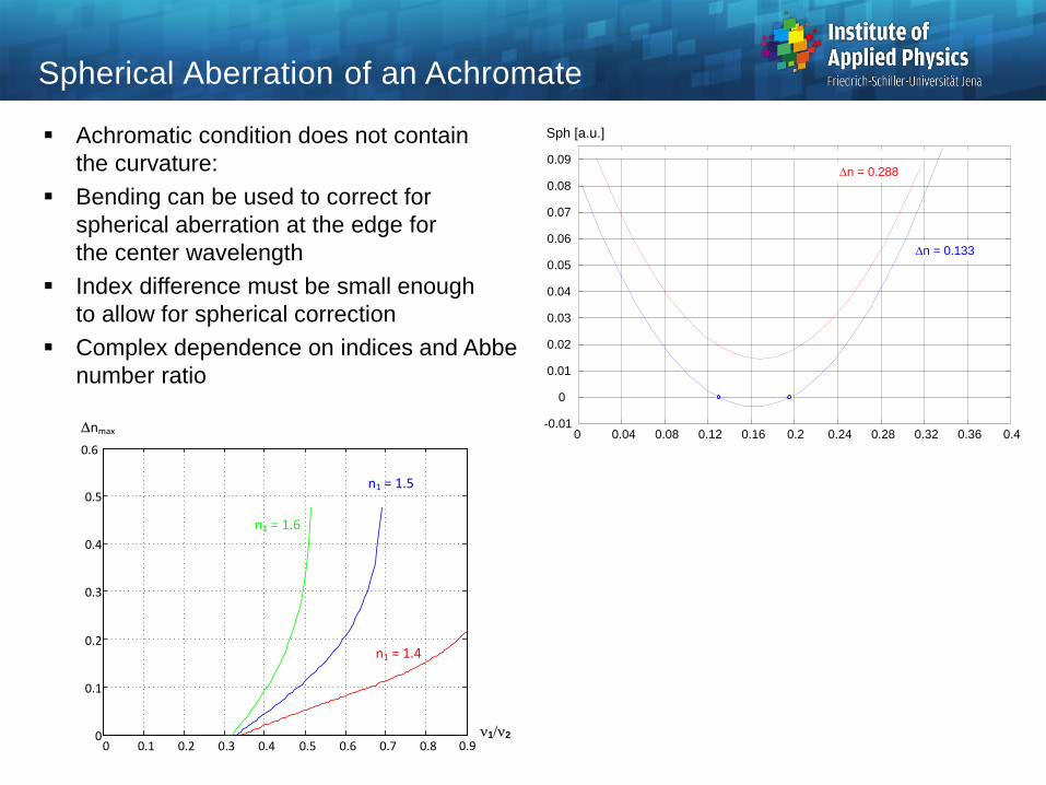
Spherical Aberration of an Achromate

Achromatic condition does not contain

the curvature:

Bending can be used to correct for

spherical aberration at the edge for

the center wavelength

Index difference must be small enough

to allow for spherical correction

Complex dependence on indices and Abbe

number ratio

-0.01

0

0.01

0.02

0.03

0.04

0.05

0.06

0.07

0.08

0.09

0 0.04 0.08 0.12 0.16 0.2 0.24 0.28 0.32 0.36 0.4

n = 0.133

n = 0.288

Sph [a.u.]

0 0.1 0.2 0.3 0.4 0.5 0.6 0.7 0.80

0.1

0.2

0.3

0.4

0.5

0.9

0.6

nmax

1/2

n1 = 1.6

n1 = 1.4

n1 = 1.5

SPH

primary

SPH

secondary

rp

SPH

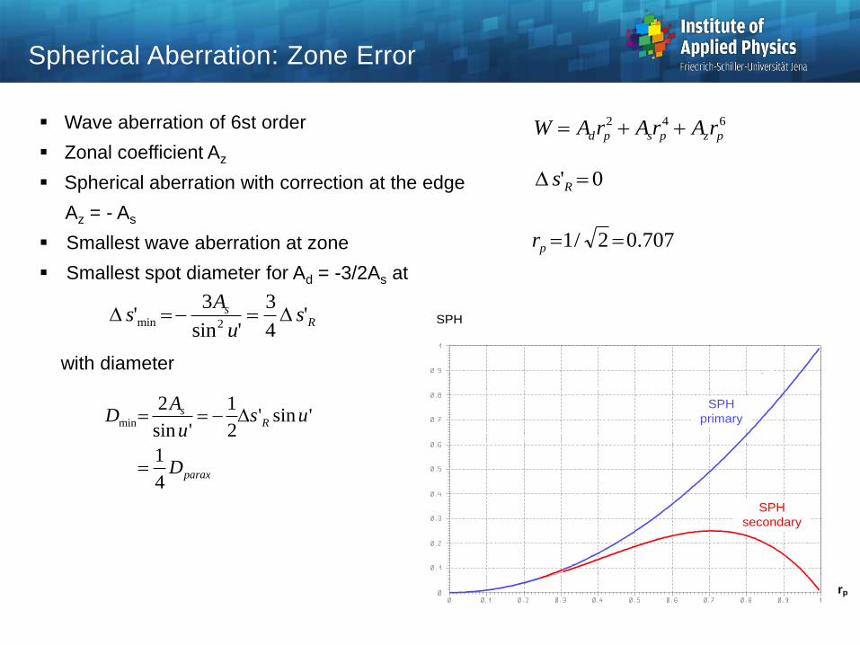
Spherical Aberration: Zone Error

Wave aberration of 6st order

Zonal coefficient Az

Spherical aberration with correction at the edge

Az = - As

Smallest wave aberration at zone

Smallest spot diameter for Ad = -3/2As at

with diameter

W A r A r A rd p s p z p 2 4 6

s R' 0

707.02/1 pr

sA

uss

R'sin '

'min 3 3

42

parax

Rs

D

usu

AD

4

1

'sin'2

1

'sin

2min

1.9 2.01.7 1.81.61.510

-6

10-4

10-5

10-3

10-2

10-1

1

10

100

Index

n

Log

Wpv

1 lens

2 lenses

3 lenses,

aplanatic / concentric

/ 4

Rayleigh 3 lenses

optimal

4 lenses

3 lenses

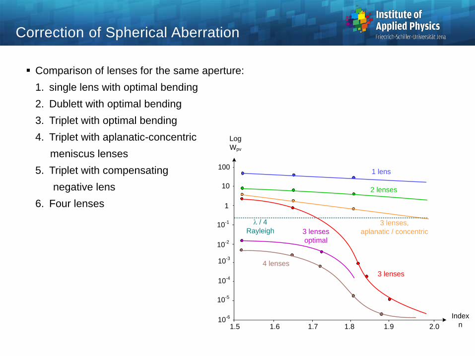
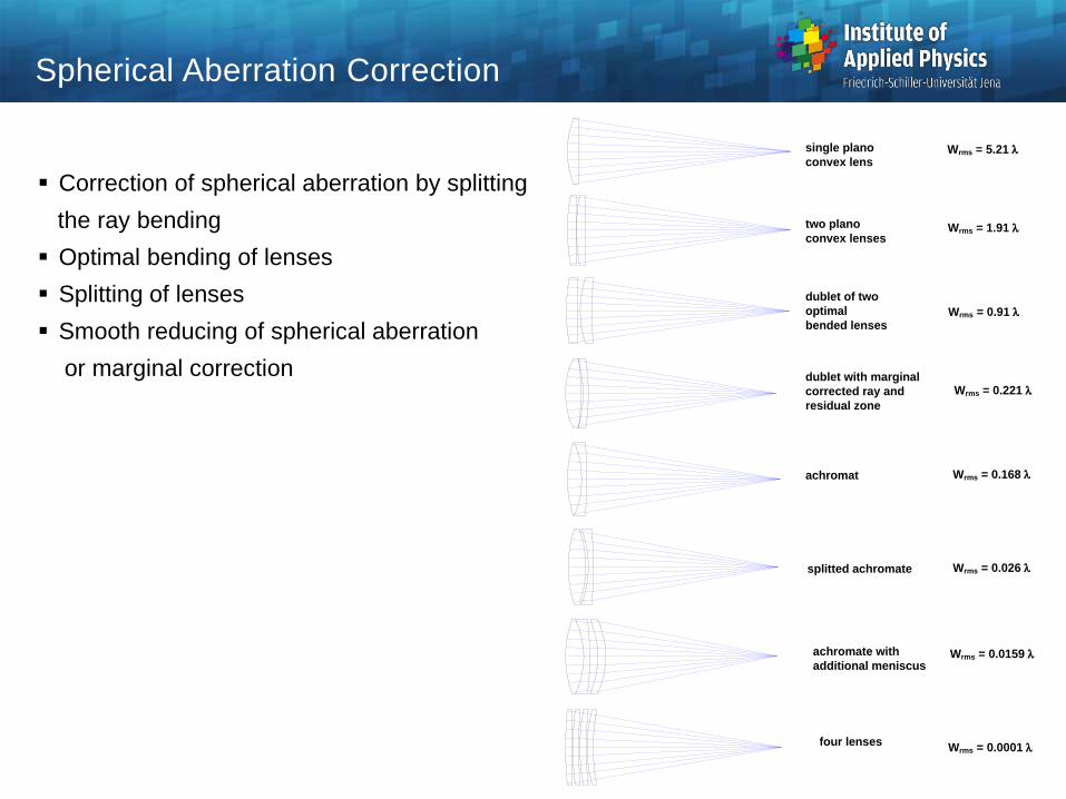
Correction of Spherical Aberration

Comparison of lenses for the same aperture:

1. single lens with optimal bending

2. Dublett with optimal bending

3. Triplet with optimal bending

4. Triplet with aplanatic-concentric

meniscus lenses

5. Triplet with compensating

negative lens

6. Four lenses

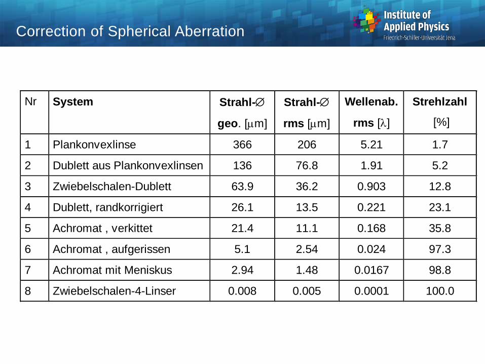
Nr System Strahl-

geo. [m]

Strahl-

rms [m]

Wellenab.

rms []

Strehlzahl

[%]

1 Plankonvexlinse 366 206 5.21 1.7

2 Dublett aus Plankonvexlinsen 136 76.8 1.91 5.2

3 Zwiebelschalen-Dublett 63.9 36.2 0.903 12.8

4 Dublett, randkorrigiert 26.1 13.5 0.221 23.1

5 Achromat , verkittet 21.4 11.1 0.168 35.8

6 Achromat , aufgerissen 5.1 2.54 0.024 97.3

7 Achromat mit Meniskus 2.94 1.48 0.0167 98.8

8 Zwiebelschalen-4-Linser 0.008 0.005 0.0001 100.0

Correction of Spherical Aberration

single plano

convex lens

two plano

convex lenses

dublet of two

optimal

bended lenses

achromat

dublet with marginal

corrected ray and

residual zone

splitted achromate

achromate with

additional meniscus

four lenses

Wrms = 5.21

Wrms = 1.91

Wrms = 0.91

Wrms = 0.221

Wrms = 0.168

Wrms = 0.026

Wrms = 0.0159

Wrms = 0.0001

Spherical Aberration Correction

Correction of spherical aberration by splitting

the ray bending

Optimal bending of lenses

Splitting of lenses

Smooth reducing of spherical aberration

or marginal correction

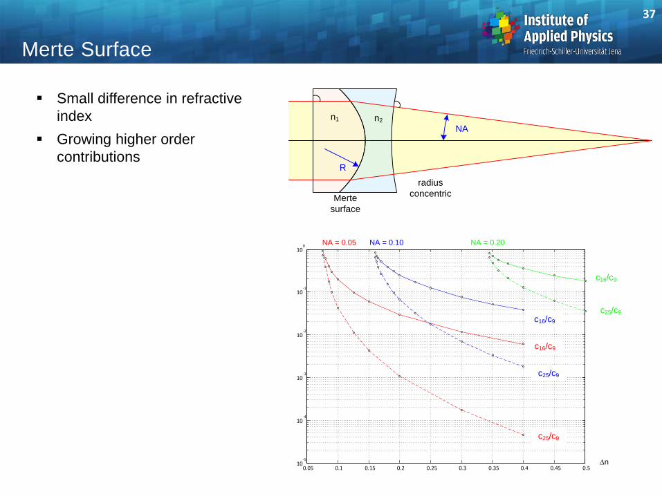
Merte Surface

Small difference in refractive

index

Growing higher order

contributions

37

n2n1

Merte

surface

radius

concentric

NA

R

0.05 0.1 0.15 0.2 0.25 0.3 0.35 0.4 0.45 0.510

-5

10-4

10-3

10-2

10-1

100

n

NA = 0.20NA = 0.05 NA = 0.10

c16/c9

c25/c9

c16/c9

c25/c9

c16/c9

c25/c9

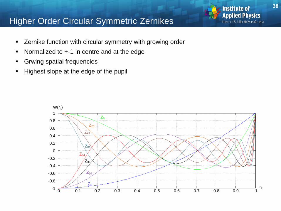
Higher Order Circular Symmetric Zernikes

Zernike function with circular symmetry with growing order

Normalized to +-1 in centre and at the edge

Grwing spatial frequencies

Highest slope at the edge of the pupil

38

W(rp)

0 0.1 0.2 0.3 0.4 0.5 0.6 0.7 0.8 0.9 1-1

-0.8

-0.6

-0.4

-0.2

0

0.2

0.4

0.6

0.8

1

rp

Z9

Z4

Z25

Z16

Z36

Z49

Z64

Z81

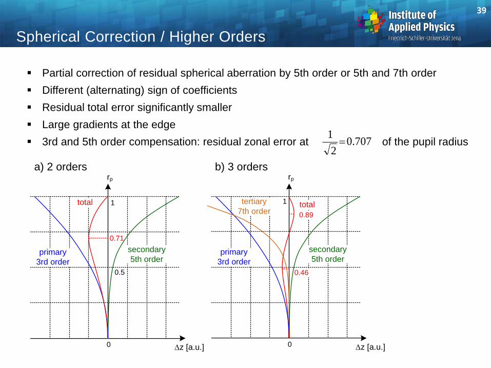
Spherical Correction / Higher Orders

Partial correction of residual spherical aberration by 5th order or 5th and 7th order

Different (alternating) sign of coefficients

Residual total error significantly smaller

Large gradients at the edge

3rd and 5th order compensation: residual zonal error at of the pupil radius

39

total

rp

z [a.u.]

primary

3rd order

secondary

5th order

1

0.5

0.71

0

total

rp

z [a.u.]

primary

3rd order

secondary

5th order

1

0.89

0

a) 2 orders b) 3 orders

0.46

tertiary

7th order

707.02

1

222

22

111 yxc

yxcz

k

1

2

b

ak

2a

bc

k

1

1

cb

k

1

1

ca

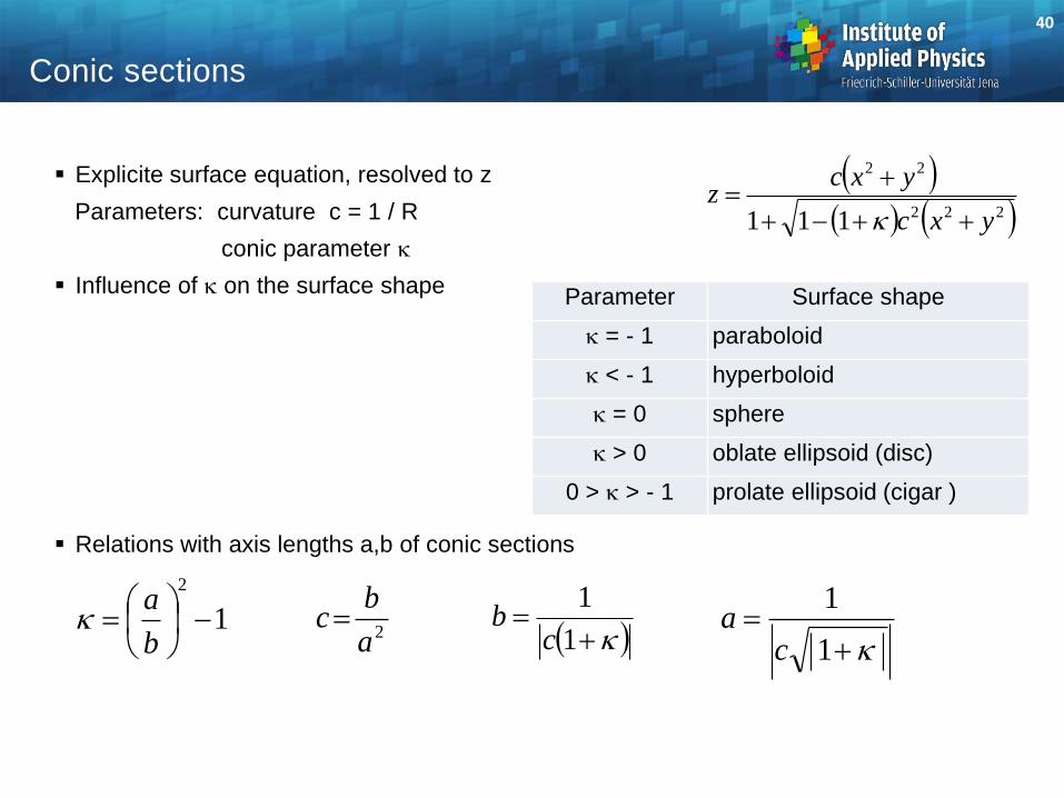
Explicite surface equation, resolved to z

Parameters: curvature c = 1 / R

conic parameter k

Influence of k on the surface shape

Relations with axis lengths a,b of conic sections

Parameter Surface shape

k = - 1 paraboloid

k < - 1 hyperboloid

k = 0 sphere

k > 0 oblate ellipsoid (disc)

0 > k > - 1 prolate ellipsoid (cigar )

40

Conic sections

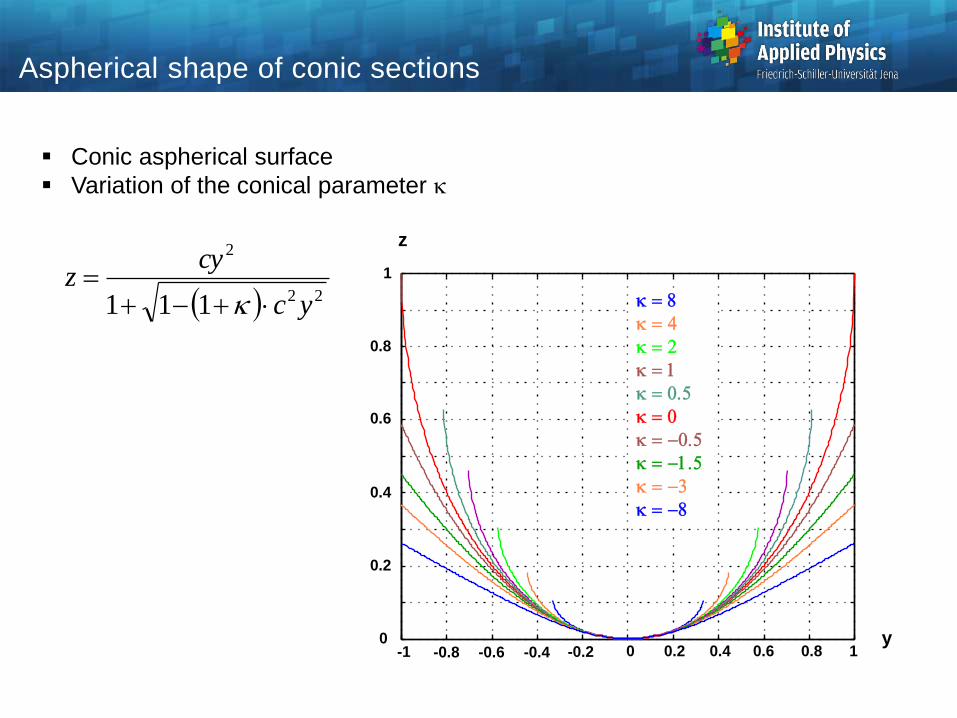
Conic aspherical surface

Variation of the conical parameter k

Aspherical shape of conic sections

z

-1 -0.8 -0.6 -0.4 -0.2 0 0.2 0.4 0.6 0.8 10

0.2

0.4

0.6

0.8

1

y

k

k

k

k

k

k

k

k

k

k

22

2

111 yc

cyz

k

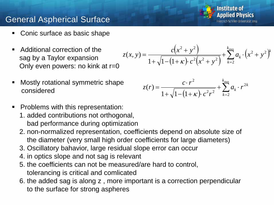
Conic surface as basic shape

Additional correction of the

sag by a Taylor expansion

Only even powers: no kink at r=0

Mostly rotational symmetric shape

considered

Problems with this representation:

1. added contributions not orthogonal,

bad performance during optimization

2. non-normalized representation, coefficients depend on absolute size of

the diameter (very small high order coefficients for large diameters)

3. Oscillatory bahavior, large residual slope error can occur

4. in optics slope and not sag is relevant

5. the coefficients can not be measured/are hard to control,

tolerancing is critical and comlicated

6. the added sag is along z , more important is a correction perpendicular

to the surface for strong aspheres

General Aspherical Surface

max

2

22

222

22

111),(

k

k

k

k yxayxc

yxcyxz

k

max

2

2

22

2

111)(

k

k

k

k rarc

rcrz

k

Aspheres - Geometry

z

y

aspherical

contour

spherical

surface

z(y)

height

y

deviation

z

sphere

z

y

perpendicular

deviation rs

deviation z

along axis

height

y

tangente

z(y)

aspherical

shape

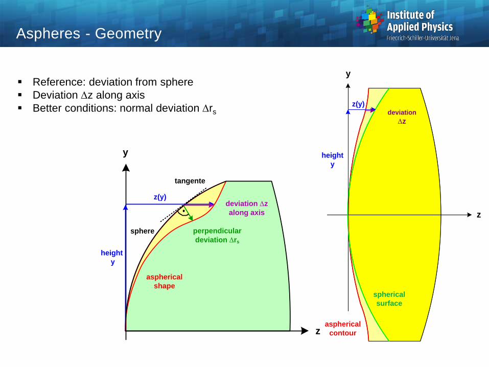
Reference: deviation from sphere

Deviation z along axis

Better conditions: normal deviation rs

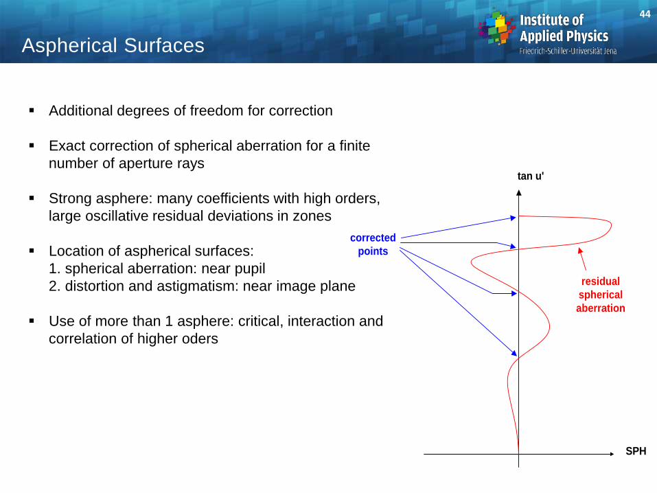
Additional degrees of freedom for correction

Exact correction of spherical aberration for a finite

number of aperture rays

Strong asphere: many coefficients with high orders,

large oscillative residual deviations in zones

Location of aspherical surfaces:

1. spherical aberration: near pupil

2. distortion and astigmatism: near image plane

Use of more than 1 asphere: critical, interaction and

correlation of higher oders

SPH

tan u'

corrected

points

residual

spherical

aberration

Aspherical Surfaces

44

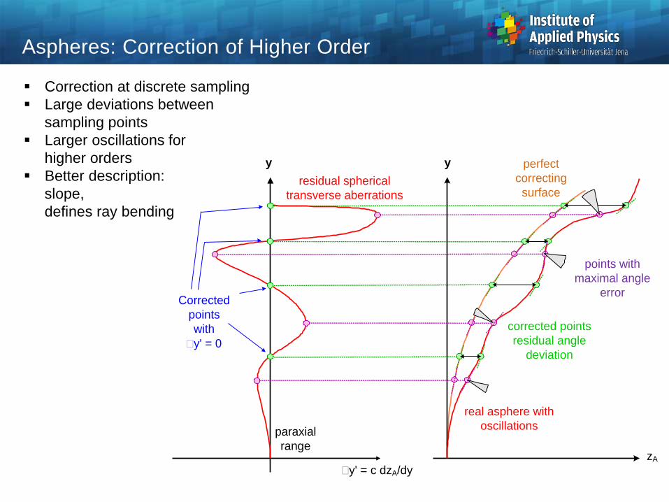
Aspheres: Correction of Higher Order

Correction at discrete sampling

Large deviations between

sampling points

Larger oscillations for

higher orders

Better description:

slope,

defines ray bending

y y

residual spherical

transverse aberrations

Corrected

points

with

�y' = 0

paraxial

range

�y' = c dzA/dy

zA

perfect

correcting

surface

corrected points

residual angle

deviation

real asphere with

oscillations

points with

maximal angle

error

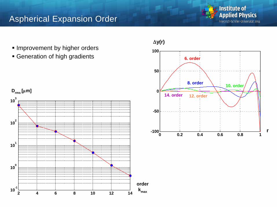
Improvement by higher orders

Generation of high gradients

Aspherical Expansion Order

r

y(r)

0 0.2 0.4 0.6 0.8 1-100

-50

0

50

100

12. order

6. order

10. order8. order

14. order

2 4 6 8 10 12 1410

-1

100

101

102

103

order

kmax

Drms

[m]

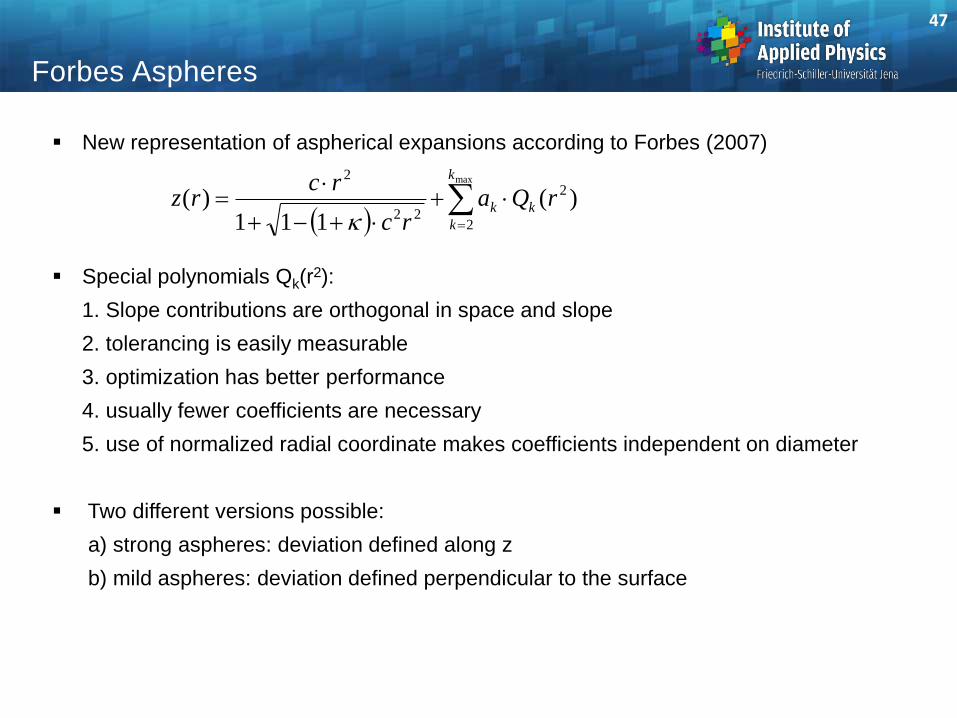
Forbes Aspheres

New representation of aspherical expansions according to Forbes (2007)

Special polynomials Qk(r2):

1. Slope contributions are orthogonal in space and slope

2. tolerancing is easily measurable

3. optimization has better performance

4. usually fewer coefficients are necessary

5. use of normalized radial coordinate makes coefficients independent on diameter

Two different versions possible:

a) strong aspheres: deviation defined along z

b) mild aspheres: deviation defined perpendicular to the surface

47

max

2

2

22

2

)(111

)(k

k

kk rQarc

rcrz

k

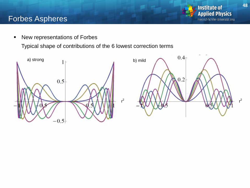
Forbes Aspheres

New representations of Forbes

Typical shape of contributions of the 6 lowest correction terms

48

r2

r2

a) strong b) mild

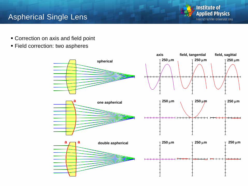
Correction on axis and field point

Field correction: two aspheres

Aspherical Single Lens

spherical

one aspherical

double aspherical

axis field, tangential field, sagittal

250 m 250 m 250 m

250 m 250 m 250 m

250 m 250 m 250 m

a

a a

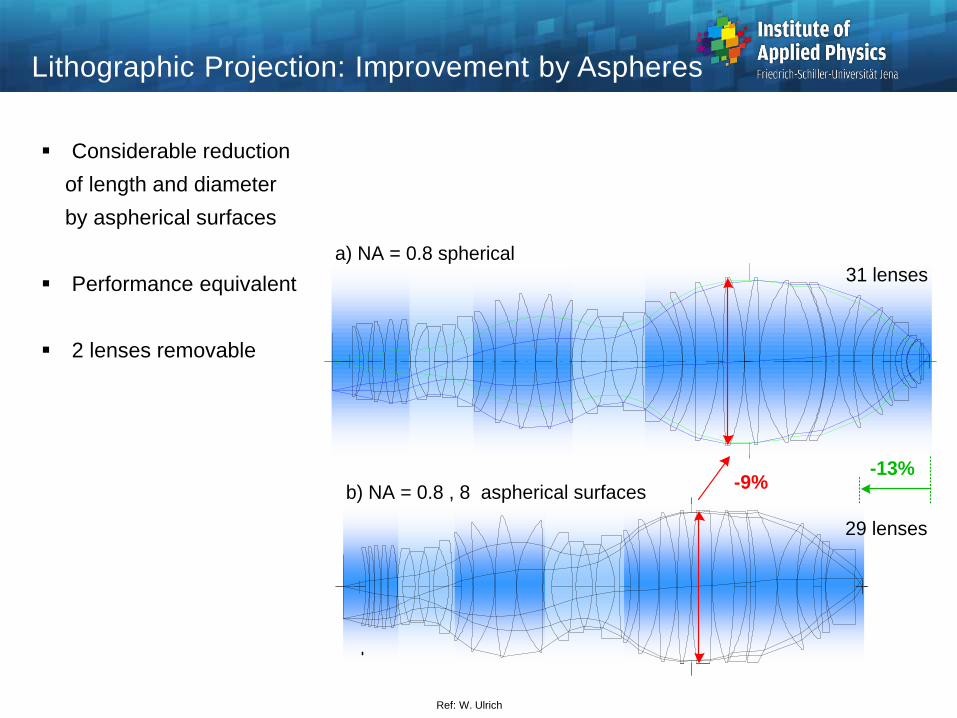
Lithographic Projection: Improvement by Aspheres

Considerable reduction

of length and diameter

by aspherical surfaces

Performance equivalent

2 lenses removable

a) NA = 0.8 spherical

b) NA = 0.8 , 8 aspherical surfaces

-13%-9%

31 lenses

29 lenses

Ref: W. Ulrich

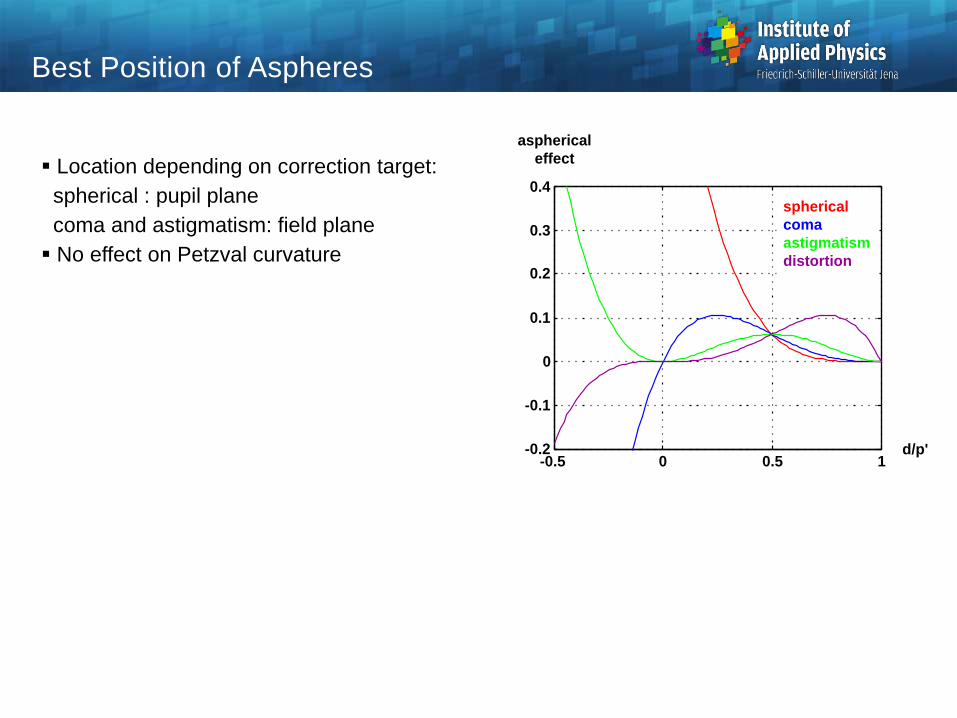
Location depending on correction target:

spherical : pupil plane

coma and astigmatism: field plane

No effect on Petzval curvature

Best Position of Aspheres

-0.5 0 0.5 1-0.2

-0.1

0

0.1

0.2

0.3

0.4

spherical

coma

astigmatism

distortion

d/p'

aspherical

effect

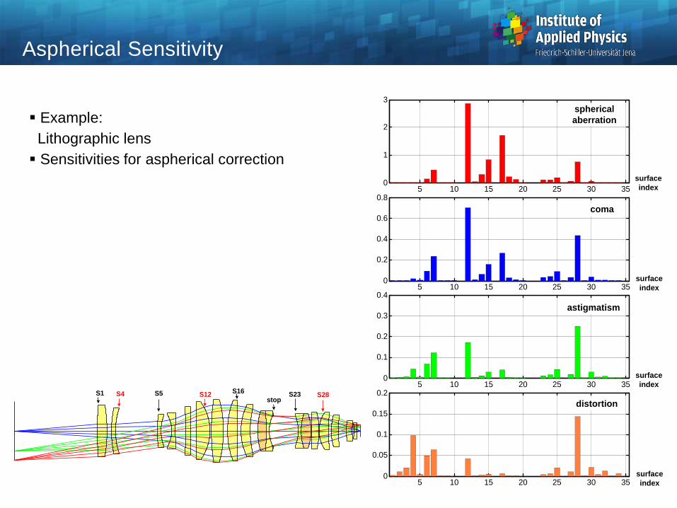
Example:

Lithographic lens

Sensitivities for aspherical correction

Aspherical Sensitivity

S1 S5 S12S16

S23 S28S4stop

5 10 15 20 25 30 350

1

2

3

5 10 15 20 25 30 350

0.2

0.4

0.6

0.8

5 10 15 20 25 30 350

0.1

0.2

0.3

0.4

5 10 15 20 25 30 350

0.05

0.1

0.15

0.2

spherical

aberration

coma

astigmatism

distortion

surface

index

surface

index

surface

index

surface

index

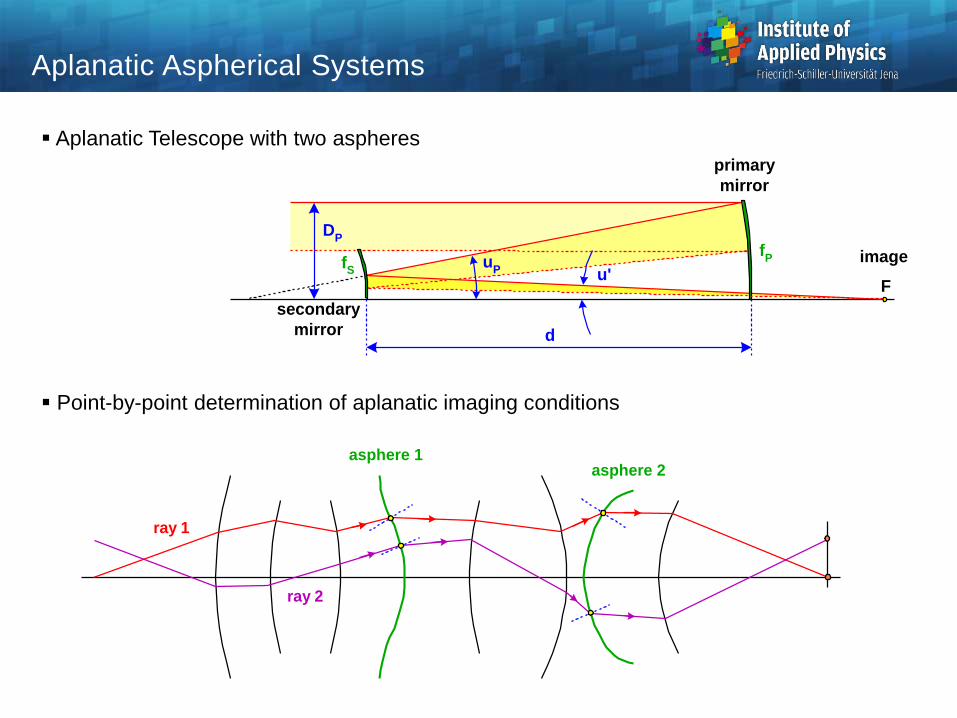
Aplanatic Telescope with two aspheres

Point-by-point determination of aplanatic imaging conditions

Aplanatic Aspherical Systems

secondary

mirror

primary

mirror

F

fP

DP

d

uP u'

fS

image

asphere 1asphere 2

ray 1

ray 2

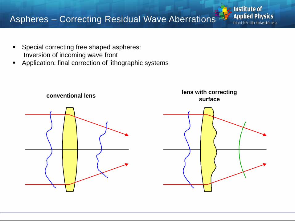
Special correcting free shaped aspheres:

Inversion of incoming wave front

Application: final correction of lithographic systems

Aspheres – Correcting Residual Wave Aberrations

conventional lenslens with correcting

surface