Image Restoration: From Sparse and Low-rank Priors to Deep Priors

Lei Zhang1, Wangmeng Zuo2

1 Dept. of computing, The Hong Kong Polytechnic University,2 School of Computer Science and Technology, Harbin Institute of Technology,

cslzhang@comp.polyu.edu.hk, wmzuo@hit.edu.cn

The use of digital imaging devices, ranging from professional digital cinema cameras to consumer grade smart-phone

cameras, has become ubiquitous. The acquired image is a degraded observation of the unknown latent image, while the

degradation comes from various factors such as noise corruption, camera shake, object motion, resolution limit, hazing, rain

streaks, or a combination of them. Image restoration (IR), as a fundamental problem in image processing and low-level

vision, aims to reconstruct the latent high quality image from its degraded observation. Image degradation is irreversible in

general, and IR is a typical ill-posed inverse problem. Due to the large space of natural image contents, prior information on

image structures is crucial to regularize the solution space and produce a good estimation of the latent image. Image prior

modeling and learning are then key issues in the IR research. This lecture-notes article describes the development of image

prior modeling and learning techniques, including sparse representation models, low-rank models, and deep learning models.

1. Relevance

IR plays an important role in many applications such as digital photography, medical image analysis, remote sensing,

surveillance and digital entertainment. We give an introduction to the major IR techniques developed in past years, and

discuss the future developments. This lecture-notes article can be used as a tutorial to IR methods for senior undergraduate

students, graduate students and researchers in the related areas. The slides associated with this lecture-notes article can be

downloaded at http://www.comp.polyu.edu.hk/∼cslzhang/IR lecture.pdf.

2. Prerequisites

Knowledge of statistical signal processing, linear algebra, and convolutional neural network will be helpful in understand-

ing the content of this lecture-notes article.

1

3. Problem Statement

Denote by x the latent image and y the degraded observation of it. A typical image degradation model can be written as

y = Hx + υ, (1)

where H denotes the degradation matrix and υ denotes the additive noise. In literature, υ is often assumed to be additive

white Gaussian noise (AWGN) with zero mean and standard deviation σ. Based on the forms of H, different IR problems

can be defined. For example, in image denoising H is an identity matrix. In image deblurring, we have Hx = k⊗ x , where

k is the blur kernel and ⊗ denotes the 2D convolution operator. In image inpainting, H is a diagonal 0-1 matrix. In image

super-resolution, H is the composition of blurring and downsampling operators.

The linear system in Eqn. (1) is generally ill-posed, i.e., we cannot obtain x by directly solving the linear system. State-of-

the-art IR methods exploit image prior information, and optimize an energy function to estimate the desired image x. From

the Bayesian perspective, Eqn. (1) defines a likelihood function P (y|x) = exp{−‖y − Hx‖22/2σ2} of x. Given the image

prior P (x), we can estimate the unknown latent image x from the observation y by maximizing the posterior probability

P (x|y), and the widely used maximum a posterior (MAP) model is

x = argmaxx {logP (x|y) ∝ (logP (y|x) + logP (x))}

= argminx{1/2‖y−Hx‖22 + λR(x)

},

(2)

whereR(x) = − logP (x) denotes the regularization term, and λ is the regularization parameter. Under the MAP framework,

one key problem is how to model the image priors P (x) (or regularizers R(x)). Successful prior models include sparse priors

and low-rank priors. Recently, deep learning techniques have also been used to learn discriminative prior models.

4. Solutions

4.1. Sparse representation

Many IR methods exploit the sparsity prior of natural images. For example, image gradient exhibits long-tailed distribu-

tion, with which the total variation (TV) methods have been widely used for solving IR problems. The wavelet transform of

an image has sparsely distributed coefficients, and thus soft-thresholding in wavelet domain is a simple yet effective denois-

ing technique. It is also found that an image patch can be well represented as the linear combination of a few atoms sparsely

selected from a dictionary. The sparse representation (a.k.a. sparse coding) based methods encode an image over an over-

complete dictionary D with `1-norm (or `p-norm, 0 ≤ p ≤ 1) sparsity regularization on the coding vector, i.e., minα ‖α‖1

s.t. x = Dα , leading to a general sparse representation based IR model:

α = argminα‖y−HDα‖+ λ‖α‖1, (3)

Eqn. (3) turns the estimation of x in Eqn. (2) into the estimation of α. Table 1 summarizes the major steps in sparse

representation based IR.

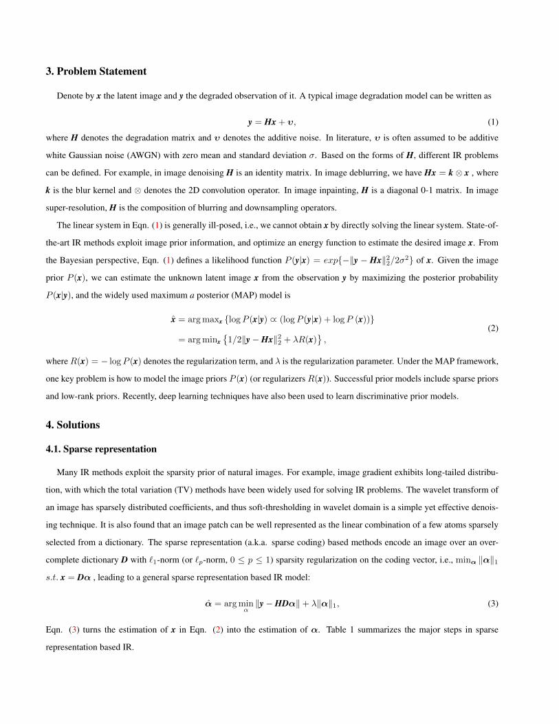
Table 1. Major steps in sparse representation based image restoration.

1. Partition the degraded image into overlapped patches.

2. For each patch, solve the nonlinear `1-norm sparse coding problem in Eqn. (3).

3. Reconstruct each patch by x = Dα.

4. Put the reconstructed patch back to the original image. For overlapped pixels between patches, average them.

5. Iterate the above procedures for a better restoration.

Figure 1. From left to right: noisy image, and the denoised images in iterations 1, 3 and 5, respectively.

Fig. 1 shows an example of image denoising by sparse representation. One can see that the noise is rapidly removed during

the iteration, and the image is well reconstructed in 5 iterations. The success of sparse representation in IR can be explained

from different perspectives. First, from the Bayesian perspective, it solves a MAP problem with a good sparsity prior.

Second, it has neuroscience explanations that the receptive fields of simple cells in primary visual cortex can be characterized

as spatially localized, oriented and bandpass. Third, from the perspective of compressed sensing, image patches are K-sparse

signals which can be well reconstructed using sparse optimization.

4.1.1 The selection of dictionary

The dictionary D plays an important role in sparse representation based IR. Early methods usually adopt some analytical

dictionaries, such as DCT bases, wavelets, curvelets, or the concatenation of them. Nonetheless, these analytically designed

dictionaries have limited capability in matching the complex natural image structures. More atoms have to be selected

to represent the given image, making the representation less sparse. To address this issue, researchers proposed to learn

dictionaries from natural images. Given a set of training samples Y = [y1, y2, . . . , yn], where yi is a vectorized patch,

dictionary learning aims to learn a dictionary D = [d1, d2, . . . , dm] from Y, where dj is an atom and m < n, such that

Y ≈ DΛ and Λ = [α1,α2, . . . ,αn] is the set of sparse codes. One classical dictionary learning method is the K-SVD [1]

algorithm, which imposes `0-norm sparsity on each coding vector αi, i = 1, 2, . . . , n.

The success of K-SVD in denoising inspired many following works, such as multi-scale dictionary learning, double sparsi-

ty, adaptive PCA dictionaries, semi-coupled dictionary learning. Sparse representation models with learned dictionaries often

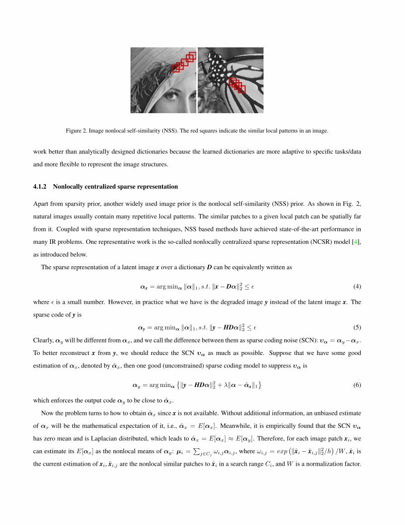
Figure 2. Image nonlocal self-similarity (NSS). The red squares indicate the similar local patterns in an image.

work better than analytically designed dictionaries because the learned dictionaries are more adaptive to specific tasks/data

and more flexible to represent the image structures.

4.1.2 Nonlocally centralized sparse representation

Apart from sparsity prior, another widely used image prior is the nonlocal self-similarity (NSS) prior. As shown in Fig. 2,

natural images usually contain many repetitive local patterns. The similar patches to a given local patch can be spatially far

from it. Coupled with sparse representation techniques, NSS based methods have achieved state-of-the-art performance in

many IR problems. One representative work is the so-called nonlocally centralized sparse representation (NCSR) model [4],

as introduced below.

The sparse representation of a latent image x over a dictionary D can be equivalently written as

αx = argminα ‖α‖1, s.t. ‖x− Dα‖22 ≤ ε (4)

where ε is a small number. However, in practice what we have is the degraded image y instead of the latent image x. The

sparse code of y is

αy = argminα ‖α‖1, s.t. ‖y−HDα‖22 ≤ ε (5)

Clearly, αy will be different from αx, and we call the difference between them as sparse coding noise (SCN): υα = αy−αx.

To better reconstruct x from y, we should reduce the SCN υα as much as possible. Suppose that we have some good

estimation of αx, denoted by αx, then one good (unconstrained) sparse coding model to suppress υα is

αy = argminα{‖y−HDα‖22 + λ‖α− αx‖1

}(6)

which enforces the output code αy to be close to αx.

Now the problem turns to how to obtain αx since x is not available. Without additional information, an unbiased estimate

of αx will be the mathematical expectation of it, i.e., αx = E[αx]. Meanwhile, it is empirically found that the SCN υα

has zero mean and is Laplacian distributed, which leads to αx = E[αx] ≈ E[αy]. Therefore, for each image patch xi, we

can estimate its E[αx] as the nonlocal means of αy: µi =∑j∈Cj ωi,jαi,j , where ωi,j = exp

(‖xi − xi,j‖22/h

)/W , xi is

the current estimation of xi, xi,j are the nonlocal similar patches to xi in a search range Ci, and W is a normalization factor.

Finally, the NCSR model becomes:

αy = argminα

{‖y−HDα‖22 + λ

N∑i=1

‖αi − µi‖1

}(7)

which can be easily solved iteratively. The NCSR model naturally integrates NSS into the sparse representation framework,

and shows competitive performance in different IR applications, including denoising, debluring and super-resolution [4].

4.2. Low-rank minimization

The sparse representation models stretch an image patch to a vector and encode it over a dictionary of one dimensional

(1D) atoms. With the NSS prior, we can have a group of similar patches as input. Group sparsity models have been proposed

to encode a group of correlated patches, whereas they are still a kind of 1D sparse coding models. An alternative way is to

format those similar patches as a matrix with each column being a stretched patch vector, and exploit the low-rank prior of

this matrix for IR.

The rank of a data matrix X counts the number of non-zero singular values of it, which is NP-hard to minimize. Alterna-

tively, the nuclear norm of X, defined as the `1-norm of its singular values ‖X‖∗ =∑i ‖σi(X)‖1, is a convex relaxation of

matrix rank function. The low-rankness of X can be viewed as a two dimensional (2D) sparsity prior. It encodes the input

2D data matrix over a set of rank-1 basis matrices, and assumes its singular values to be sparsely distributed, i.e., it has only

a few non-zero or significant singular values.

Let Y be a matrix of degraded image patches. The latent low-rank matrix X can be estimated form Y via the following

nuclear norm minimization (NNM) problem

X = argminX ‖Y − X‖2F + λ‖X‖∗ (8)

Cai et al. [2] showed that Eqn. (8) has a closed-form solution

X = USλ2(Σ)VT , (9)

where Y = UΣVT is the SVD of Y and Sλ2(Σ)ii = max(Σii − λ

2 , 0) is the singular value thresholding operator.

4.2.1 Weighted nuclear norm minimization

The NNM mentioned above has shown interesting results on image and video denoising. As can be seen from Eqn. (9),

however, it shrinks all the singular values equally by the threshold λ, ignoring the different significances of matrix singular

values. It is known that the larger singular values can be more important to represent the latent data in many applications. In

[6], a weighted nuclear norm is defined:

‖X‖w,∗ =∑i ‖wiσi(X)‖1, (10)

where wi is the weight assigned on singular value σi(X). A weighted nuclear norm minimization (WNNM) model is then

presented [6] to recover the latent data matrix X from Y

X = argminX ‖Y − X‖2F + ‖X‖w,∗. (11)

5

Different from the convex NNM model in Eqn. (11), the WNNM model in Eqn. (15) becomes

non-convex. Fortunately and interestingly, it is proved in [18] that WNNM still has a globally

optimal solution, as given in the following Theorem 1.

Theorem 1. ∀𝒀∈𝑅^(𝑚×𝑛), let 𝒀=𝑼𝜮𝑽^𝑇 be its SVD. The optimal solution of the WNNM

problem in Eqn. (15) is 𝑿 = 𝑼𝑫𝑽^𝑇, where 𝑫 is a diagonal matrix with diagonal entries 𝒅=[𝑑_1,

𝑑_2,…,𝑑_𝑟] (𝑟=𝑚𝑖𝑛(𝑚,𝑛)) determined by:

〖𝑚𝑖𝑛〗_(𝑑_1," " 𝑑_2…𝑑_𝑛 ) ∑2_(𝑖=1)^𝑟▒〖〖〖(𝑑〗_𝑖−𝜎_𝑖)〗^2+𝑤_𝑖 〗 𝑑_𝑖 𝑠.𝑡. 𝑑_1

〖≥𝑑〗_2≥𝑑_𝑟≥

It is also shown in [18] that when the weights wi are in a non-ascending order, WNNM has a

closed-form solution, as given in the following Corollary 1.

Corollary 1. If the weights satisfy 〖0≤" " 𝑤〗_1 〖≤" " 𝑤〗_2≤𝑤_𝑛, the non-convex

WNNM problem has a closed form optimal solution 𝑿 =𝑼𝑆_𝑤 〖(𝜮)𝑽〗^𝑇, where 𝒀=𝑼𝜮𝑽^𝑇 is

the SVD of 𝒀, and 𝑆_𝑤 (𝜮)〗_𝑖𝑖= 𝑚𝑎𝑥(𝜮_𝑖𝑖−𝑤_𝑖

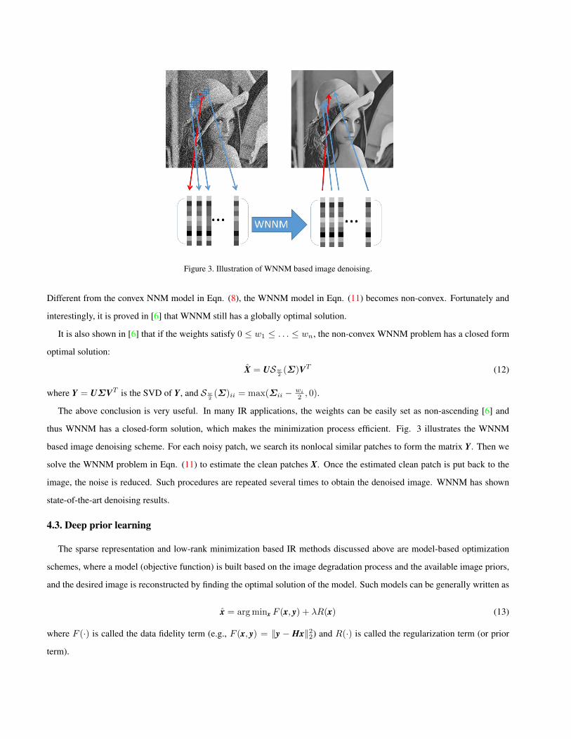
Figure 3. Illustration of WNNM based image denoising.

Corollary 1 is very useful. In many IR applications, the weights can be easily set as non-

ascending [18] and thus WNNM has a closed-form solution, which makes the minimization process

efficient. Fig. 3 illustrates the WNNM based image denoising scheme. For each noisy patch, we

search its nonlocal similar patches to form matrix 𝒀. Then we solve the WNNM problem Eqn. (15)

to estimate the clean patches 𝑿. Put the estimated clean patch back to the image, the noise is

reduced. Such procedures are repeated several times to obtain the denoised image. WNNM has

shown very competitive denoising results.

Deep prior learning

The sparse representation and low-rank minimization based IR methods discussed above are model

based optimization schemes, where a model (objective function) is built based on the image

degradation process and the available image priors, and the desired image is reconstructed by

finding the optimal solution of the model. Such models can be generally written as

(16)

where F() is called the data fidelity term (e.g., F(x,y)=||y-Hx||^2_2) and R() is called the

regularization term (or prior term).

Another category of IR methods is the so-called discriminative learning methods, which learn a

compact inference or a mapping function from a training set of degraded-latent image pairs. The

general model of discriminative learning methods can be written as

(17)

Figure 3. Illustration of WNNM based image denoising.

Different from the convex NNM model in Eqn. (8), the WNNM model in Eqn. (11) becomes non-convex. Fortunately and

interestingly, it is proved in [6] that WNNM still has a globally optimal solution.

It is also shown in [6] that if the weights satisfy 0 ≤ w1 ≤ . . . ≤ wn, the non-convex WNNM problem has a closed form

optimal solution:

X = USw2(Σ)VT (12)

where Y = UΣVT is the SVD of Y, and Sw2(Σ)ii = max(Σii − wi

2 , 0).

The above conclusion is very useful. In many IR applications, the weights can be easily set as non-ascending [6] and

thus WNNM has a closed-form solution, which makes the minimization process efficient. Fig. 3 illustrates the WNNM

based image denoising scheme. For each noisy patch, we search its nonlocal similar patches to form the matrix Y. Then we

solve the WNNM problem in Eqn. (11) to estimate the clean patches X. Once the estimated clean patch is put back to the

image, the noise is reduced. Such procedures are repeated several times to obtain the denoised image. WNNM has shown

state-of-the-art denoising results.

4.3. Deep prior learning

The sparse representation and low-rank minimization based IR methods discussed above are model-based optimization

schemes, where a model (objective function) is built based on the image degradation process and the available image priors,

and the desired image is reconstructed by finding the optimal solution of the model. Such models can be generally written as

x = argminx F (x, y) + λR(x) (13)

where F (·) is called the data fidelity term (e.g., F (x, y) = ‖y − Hx‖22) and R(·) is called the regularization term (or prior

term).

Another category of IR methods is the so-called discriminative learning methods, which learn a compact inference or a

mapping function from a training set of degraded-latent image pairs. The general model of discriminative learning methods

can be written as

minΘ loss(x, x), s.t. x = F(y,H;Θ) (14)

where F(·) is the inference or mapping function with parameter set Θ, and loss(·) is the loss function to measure the

similarity between output image x and ground-truth image x. The recently developed deep learning based IR methods

[3, 7, 10, 8, 9] are typical discriminative learning methods, where F(·) is a deep convolutional neural network (CNN).

4.3.1 Deep CNNs for IR

One of the first CNN based IR methods is the SRCNN (super-resolution CNN) method [3] for single image super-resolution

(SISR). It is actually modestly deep because it has only 2 hidden layers. A truly deep CNN for SISR was developed in [7].

The so-called VDSR method first initializes the low-resolution (LR) image to a high-resolution (HR) image (e.g., by bi-cubic

interpolation), and then learns a CNN to predict the residual between the initialized HR image and the ground-truth image.

VDSR shows highly competitive PSNR results, and it demonstrates that a single CNN can perform SISR with multiple

scaling factors.

VDSR enlarges the LR input to the same size of the HR image before goes through a CNN. This not only restricts the

area of receptive fields but also increases the cost of convolution operations in CNN. A more efficient solution is to directly

predict the missing HR pixels from the LR image, as proposed in [9]. The so-called efficient sub-pixel CNN (ESPCNN)

learns to predict the feature maps of each sub-image, and aggregates the sub-images into the final HR image.

Most existing SISR methods use the mean squared error (MSE) as the loss function to optimize the network parameters

Θ. Minimizing MSE tends to produce the mean image of possible observations. As a result, the output HR image can be

over-smoothed without a good perceptual quality. Inspired by the great success of recently developed Generative Adversarial

Nets (GAN) [5], a perceptual loss function, which consists of a content loss (i.e., MSE) and a GAN based adversarial loss, is

proposed in [8] to generate the HR images. Though the PSNR index is not very high, the so-call SRGAN method produces

perceptually very pleasant SISR results.

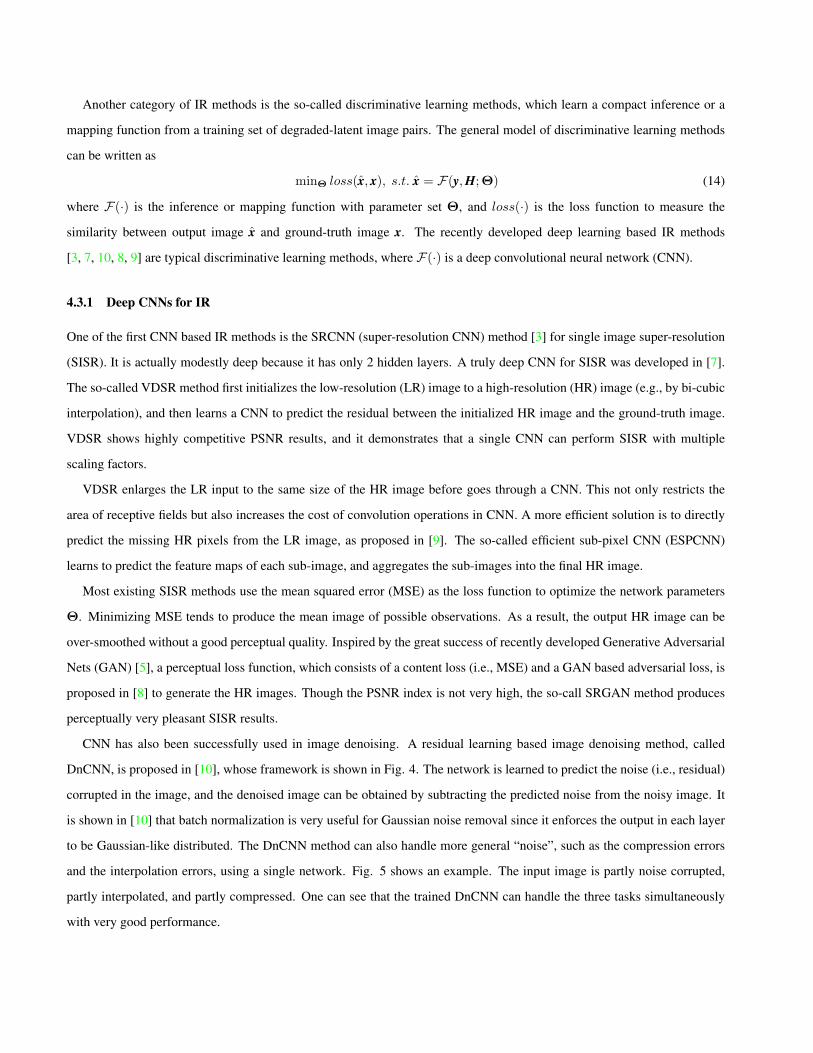
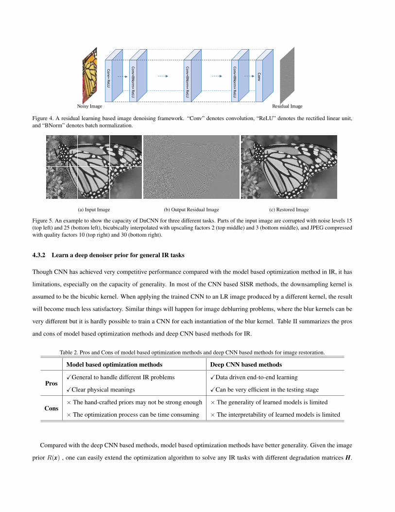
CNN has also been successfully used in image denoising. A residual learning based image denoising method, called

DnCNN, is proposed in [10], whose framework is shown in Fig. 4. The network is learned to predict the noise (i.e., residual)

corrupted in the image, and the denoised image can be obtained by subtracting the predicted noise from the noisy image. It

is shown in [10] that batch normalization is very useful for Gaussian noise removal since it enforces the output in each layer

to be Gaussian-like distributed. The DnCNN method can also handle more general “noise”, such as the compression errors

and the interpolation errors, using a single network. Fig. 5 shows an example. The input image is partly noise corrupted,

partly interpolated, and partly compressed. One can see that the trained DnCNN can handle the three tasks simultaneously

with very good performance.

Noisy Image Residual Image

Co

nv+ ReLU

Co

nv+BN

orm

+ ReLU

Co

nv+BN

orm

+ ReLU

Co

nv+BN

orm

+ ReLU

Conv

Figure 4. A residual learning based image denoising framework. “Conv” denotes convolution, “ReLU” denotes the rectified linear unit,and “BNorm” denotes batch normalization.

(a) Input Image (b) Output Residual Image (c) Restored Image

Figure 5. An example to show the capacity of DnCNN for three different tasks. Parts of the input image are corrupted with noise levels 15(top left) and 25 (bottom left), bicubically interpolated with upscaling factors 2 (top middle) and 3 (bottom middle), and JPEG compressedwith quality factors 10 (top right) and 30 (bottom right).

4.3.2 Learn a deep denoiser prior for general IR tasks

Though CNN has achieved very competitive performance compared with the model based optimization method in IR, it has

limitations, especially on the capacity of generality. In most of the CNN based SISR methods, the downsampling kernel is

assumed to be the bicubic kernel. When applying the trained CNN to an LR image produced by a different kernel, the result

will become much less satisfactory. Similar things will happen for image deblurring problems, where the blur kernels can be

very different but it is hardly possible to train a CNN for each instantiation of the blur kernel. Table II summarizes the pros

and cons of model based optimization methods and deep CNN based methods for IR.

Table 2. Pros and Cons of model based optimization methods and deep CNN based methods for image restoration.

Model based optimization methods Deep CNN based methods

ProsXGeneral to handle different IR problems XData driven end-to-end learning

XClear physical meanings XCan be very efficient in the testing stage

Cons× The hand-crafted priors may not be strong enough × The generality of learned models is limited

× The optimization process can be time consuming × The interpretability of learned models is limited

Compared with the deep CNN based methods, model based optimization methods have better generality. Given the image

prior R(x) , one can easily extend the optimization algorithm to solve any IR tasks with different degradation matrices H.

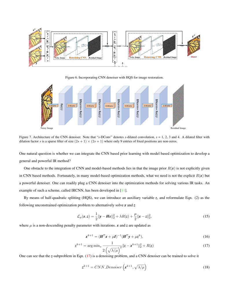
Figure 6. Incorporating CNN denoiser with HQS for image restoration.

Noisy Image Residual Image

ReLU

BN

orm

+ ReLU

BN

orm

+ ReLU

BN

orm

+ ReLU

BN

orm

+ ReLU

BN

orm

+ ReLU

1-DConv2-DConv 2-DConv3-DConv 3-DConv4-DConv1-DConv

Figure 7. Architecture of the CNN denoiser. Note that “s-DConv” denotes s-dilated convolution, s = 1, 2, 3 and 4. A dilated filter withdilation factor s is a sparse filter of size (2s+ 1)× (2s+ 1) where only 9 entries of fixed positions are non-zeros.

One natural question is whether we can integrate the CNN based prior learning with model based optimization to develop a

general and powerful IR method?

One obstacle to the integration of CNN and model-based methods lies in that the image prior R(x) is not explicitly given

in CNN based methods. Fortunately, in many model-based optimization methods, what we need is not the explicit R(x) but

a powerful denoiser. One can readily plug a CNN denoiser into the optimization methods for solving various IR tasks. An

example of such a scheme, called IRCNN, has been developed in [11].

By means of half-quadratic splitting (HQS), we can introduce an auxiliary variable z, and reformulate Eqn. (2) as the

following unconstrained optimization problem to alternatively solve x and z

Lµ(x, z) =1

2‖y−Hx‖22 + λR(z) +

µ

2‖x− z‖22, (15)

where µ is a non-descending penalty parameter with iterations. x and z are updated as

xk+1 = (HT x + µI)−1(HT y + µzk), (16)

zk+1 = argminz1

2(√

λ/µ)2 ‖z− xk+1‖22 +R(z) (17)

One can see that the z-subproblem in Eqn. (17) is a denoising problem, and a CNN denoiser can be trained to solve it

zk+1 = CNN Denoiser(

xk+1,√λ/µ

)(18)

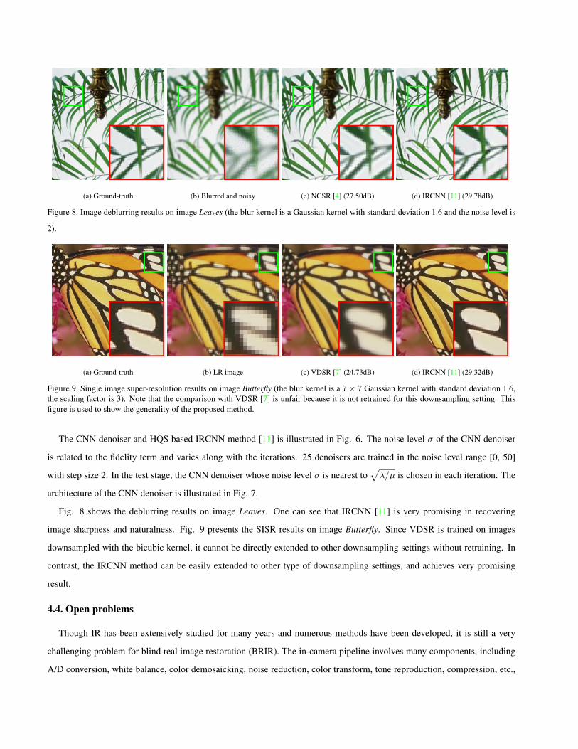
(a) Ground-truth (b) Blurred and noisy (c) NCSR [4] (27.50dB) (d) IRCNN [11] (29.78dB)

Figure 8. Image deblurring results on image Leaves (the blur kernel is a Gaussian kernel with standard deviation 1.6 and the noise level is

2).

(a) Ground-truth (b) LR image (c) VDSR [7] (24.73dB) (d) IRCNN [11] (29.32dB)

Figure 9. Single image super-resolution results on image Butterfly (the blur kernel is a 7× 7 Gaussian kernel with standard deviation 1.6,the scaling factor is 3). Note that the comparison with VDSR [7] is unfair because it is not retrained for this downsampling setting. Thisfigure is used to show the generality of the proposed method.

The CNN denoiser and HQS based IRCNN method [11] is illustrated in Fig. 6. The noise level σ of the CNN denoiser

is related to the fidelity term and varies along with the iterations. 25 denoisers are trained in the noise level range [0, 50]

with step size 2. In the test stage, the CNN denoiser whose noise level σ is nearest to√λ/µ is chosen in each iteration. The

architecture of the CNN denoiser is illustrated in Fig. 7.

Fig. 8 shows the deblurring results on image Leaves. One can see that IRCNN [11] is very promising in recovering

image sharpness and naturalness. Fig. 9 presents the SISR results on image Butterfly. Since VDSR is trained on images

downsampled with the bicubic kernel, it cannot be directly extended to other downsampling settings without retraining. In

contrast, the IRCNN method can be easily extended to other type of downsampling settings, and achieves very promising

result.

4.4. Open problems

Though IR has been extensively studied for many years and numerous methods have been developed, it is still a very

challenging problem for blind real image restoration (BRIR). The in-camera pipeline involves many components, including

A/D conversion, white balance, color demosaicking, noise reduction, color transform, tone reproduction, compression, etc.,

9

(a) Ground-truth (b) Blurred and noisy (c) NCSR [15] (??dB) (d) IRCNN [25] (??dB)

Figure 8. Image deblurring results on image Leaves (the blur kernel is Gaussian kernel with standard deviation ??

and the noise level is ??).

(a) Groundtruth (b) LR image c) VDSR [20] (24.73dB) (d) IRCNN [25] (29.32dB)

Figure 9. Single image super-resolution results on image Butterfly (the blur kernel is 7×7 Gaussian kernel with

standard deviation 1.6, the scaling factor is 3). Note that the comparison with VDSR [20] is unfair because it is

not retrained for this downsampling setting. This figure is used to show the generality of the proposed method.

Open problems Though IR has been extensively studied for many years and numerous methods have been

developed, it is still a very challenging problem for blind real image restoration (BRIR). The in-

camera pipeline involves many components, including A/D conversion, white balance, color

demosaicking, noise reduction, color transform, tone reproduction, compression, etc., and the

quality of final output image is subject to many external and internal factors, including illumination,

lens, CCD/CMOS sensors, exposure, ISO, camera shaking and object motion, etc. The degradations

in real images are too complex to be described by simple models such as y = Hx + v. Fig. 10 shows

two real world low quality images, which are hard to be satisfactorily reconstructed by all existing

IR methods. The noise therein is strong, non-Gaussian and signal dependent, while the image is

low-resolution with non-uniform blur and compression artifacts.

Figure 10. Two real world low quality images.

Will deep learning a potential good solution to the challenging BRIR problem? We would like to

give a positive answer to this question, yet one critical issue is how we can collect the degraded and

ground-truth image pairs for training? Note that most of the existing deep CNN based IR methods

are supervised learning methods with simulated training data. AWGN is added to the clean images

to simulate the noisy images, and high resolution images are downsampled to simulate the low-

Figure 10. Two real world low quality images.

and the quality of a final output image is subjected to many external and internal factors, including illumination, lens, C-

CD/CMOS sensors, exposure, ISO, camera shaking and object motion, etc. The degradations in real world images are too

complex to be described by simple models such as y = Hx + υ. Fig. 10 shows two real world low quality images, which

are hard to be satisfactorily reconstructed by all existing IR methods. The noise therein is strong, non-Gaussian and signal

dependent, while the image is low-resolution with non-uniform blur and compression artifacts.

Will deep learning be a good solution to the challenging BRIR problem? We would like to give a positive answer to this

question, yet one critical issue is how we can collect the degraded and ground-truth image pairs for training. Note that most

of the existing deep CNN based IR methods are supervised learning methods with simulated training data. AWGN is added

to the clean images to simulate the noisy images, and high resolution images are downsampled to simulate the low-resolution

images. However, the CNNs trained by such simulated image pairs are much less effective to process the real world degraded

images.

How can we train deep models for IR without paired data? Are the recently developed GAN techniques [5] able to tackle

this challenging issue? We leave those questions as open problems for future investigations.

5. What we have learned

We introduced the recent developments of sparse representation, low-rank minimization and deep learning (more specif-

ically deep CNN) based IR methods. While the image sparsity and low-rankness priors have been dominantly used in past

decades, the CNN based models have been recently rapidly developed to learn deep image priors and have shown promising

performance. However, there remain many challenging and interesting problems to investigate for deep learning based IR.

One key issue is the lack of training image pairs in real-world IR applications. It is still an open problem to train deep IR

models without using image pairs.

6. Authors

Lei Zhang (cslzhang@comp.polyu.edu.hk) is a Full Professor of Department of Computing at the Hong Kong Polytechnic

University. His research interests include image enhancement and restoration, image quality assessment, image classification,

object detection and visual tracking. He is a Web of Science Highly Cited Researcher selected by Thomson Reuters.

Wangmeng Zuo (wmzuo@hit.edu.cn) is a Full Professor of School of Computer Science and Technology at Harbin In-

stitute of Technology. His research interests include image enhancement and restoration, image generation, visual tracking,

convolutional network, and image classification. He is a Senior Member of the IEEE.

References

[1] M. Aharon, M. Elad, and A. Bruckstein. K-svd: An algorithm for designing overcomplete dictionaries for sparse representation.

IEEE Transactions on Signal Processing, 54(11):4311–4322, 2006. 3

[2] J.-F. Cai, E. J. Candes, and Z. Shen. A singular value thresholding algorithm for matrix completion. SIAM Journal on Optimization,

20(4):1956–1982, 2010. 5

[3] C. Dong, C. C. Loy, K. He, and X. Tang. Image super-resolution using deep convolutional networks. IEEE Transactions on Pattern

Analysis and Machine Intelligence, 38(2):295–307, 2016. 7

[4] W. Dong, L. Zhang, G. Shi, and X. Li. Nonlocally centralized sparse representation for image restoration. IEEE Transactions on

Image Processing, 22(4):1620–1630, 2013. 4, 5, 10

[5] I. Goodfellow, J. Pouget-Abadie, M. Mirza, B. Xu, D. Warde-Farley, S. Ozair, A. Courville, and Y. Bengio. Generative adversarial

nets. In Advances in Neural Information Processing Systems, pages 2672–2680, 2014. 7, 11

[6] S. Gu, Q. Xie, D. Meng, W. Zuo, X. Feng, and L. Zhang. Weighted nuclear norm minimization and its applications to low level

vision. International Journal of Computer Vision, 121(2):183–208, 2017. 5, 6

[7] J. Kim, J. Kwon Lee, and K. Mu Lee. Accurate image super-resolution using very deep convolutional networks. In IEEE Conference

on Computer Vision and Pattern Recognition, pages 1646–1654, 2016. 7, 10

[8] C. Ledig, L. Theis, F. Huszar, J. Caballero, A. Cunningham, A. Acosta, A. Aitken, A. Tejani, J. Totz, Z. Wang, et al. Photo-

realistic single image super-resolution using a generative adversarial network. In IEEE Conference on Computer Vision and Pattern

Recognition, 2017. 7

[9] W. Shi, J. Caballero, F. Huszar, J. Totz, A. P. Aitken, R. Bishop, D. Rueckert, and Z. Wang. Real-time single image and video

super-resolution using an efficient sub-pixel convolutional neural network. In IEEE Conference on Computer Vision and Pattern

Recognition, pages 1874–1883, 2016. 7

[10] K. Zhang, W. Zuo, Y. Chen, D. Meng, and L. Zhang. Beyond a gaussian denoiser: Residual learning of deep cnn for image denoising.

IEEE Transactions on Image Processing, 7(26):3142 – 3155, 2017. 7

[11] K. Zhang, W. Zuo, S. Gu, and L. Zhang. Learning deep cnn denoiser prior for image restoration. In IEEE Conference on Computer

Vision and Pattern Recognition, 2017. 9, 10