Image Restoration: From Sparse and Low-rank Priors to

Deep Priors

Lei ZhangDept. of Computing

The Hong Kong Polytechnic Universityhttp://www.comp.polyu.edu.hk/~cslzhang

1

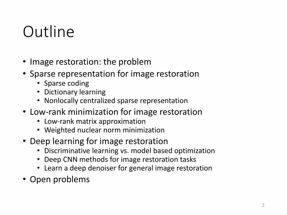
Outline

• Image restoration: the problem

• Sparse representation for image restoration• Sparse coding• Dictionary learning• Nonlocally centralized sparse representation

• Low-rank minimization for image restoration• Low-rank matrix approximation • Weighted nuclear norm minimization

• Deep learning for image restoration• Discriminative learning vs. model based optimization• Deep CNN methods for image restoration tasks• Learn a deep denoiser for general image restoration

• Open problems

2

Image restoration: the problem

3

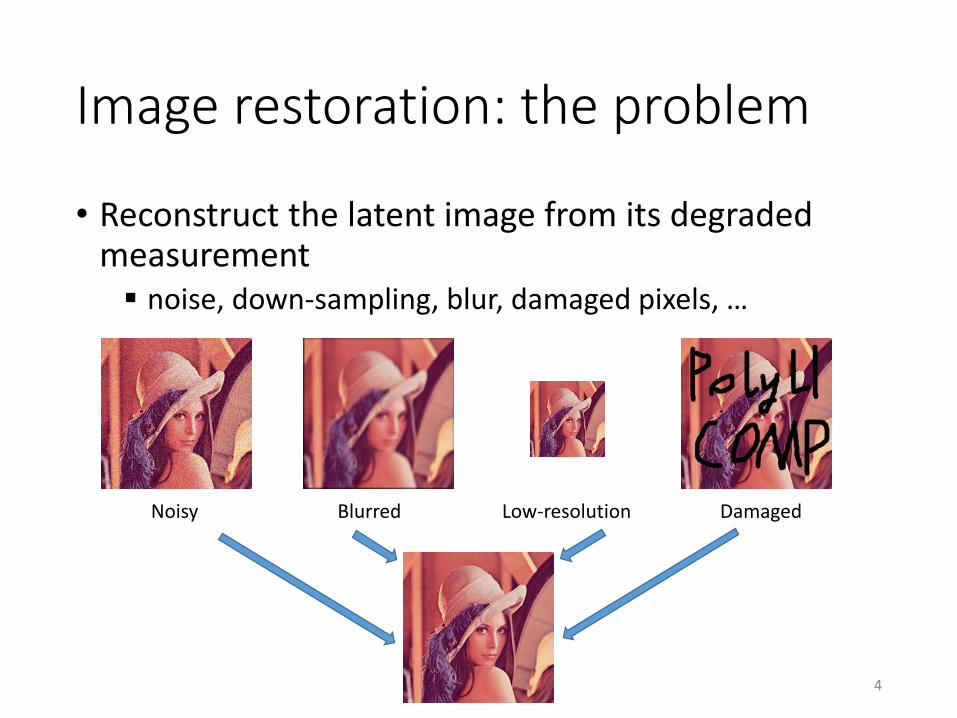
Image restoration: the problem

• Reconstruct the latent image from its degraded measurement noise, down-sampling, blur, damaged pixels, …

4

Noisy Blurred Low-resolution Damaged

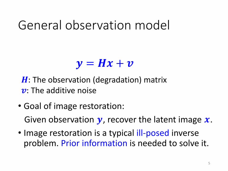
General observation model

• Goal of image restoration:

Given observation 𝒚, recover the latent image 𝒙.

• Image restoration is a typical ill-posed inverse problem. Prior information is needed to solve it.

𝒚 = 𝑯𝒙 + 𝒗

𝑯: The observation (degradation) matrix𝒗: The additive noise

5

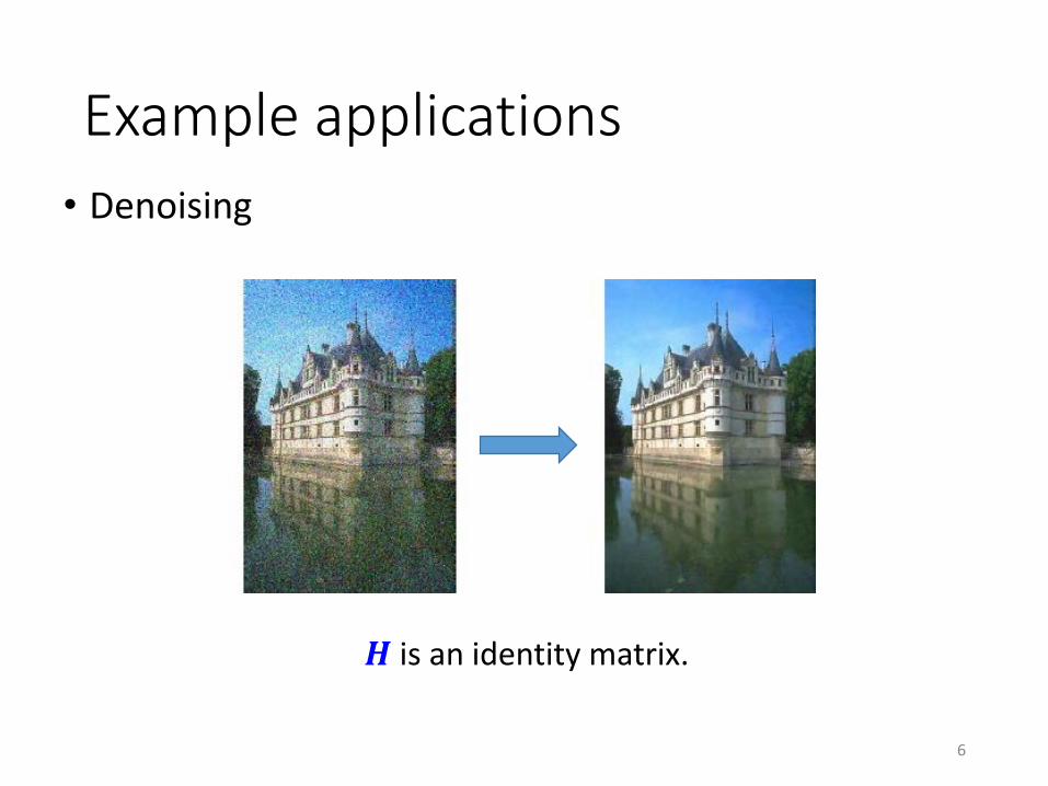
Example applications

• Denoising

6

𝑯 is an identity matrix.

Example applications

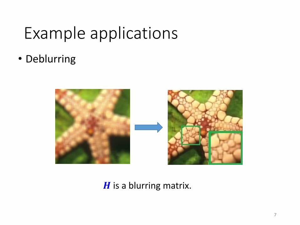
• Deblurring

7

𝑯 is a blurring matrix.

Example applications

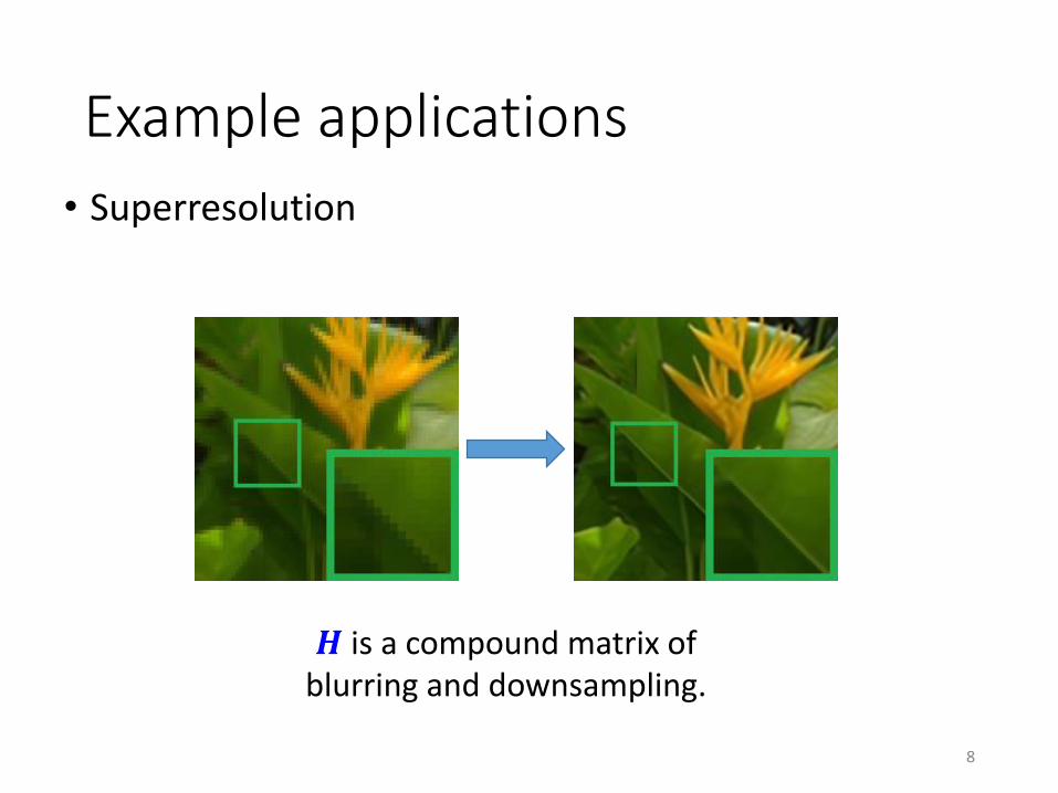
• Superresolution

8

𝑯 is a compound matrix of blurring and downsampling.

Example applications

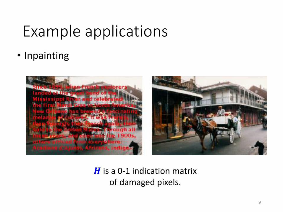
• Inpainting

9

𝑯 is a 0-1 indication matrix of damaged pixels.

Example applications

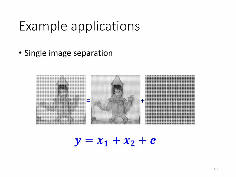
• Single image separation

10

= +

𝒚 = 𝒙𝟏 + 𝒙𝟐 + 𝒆

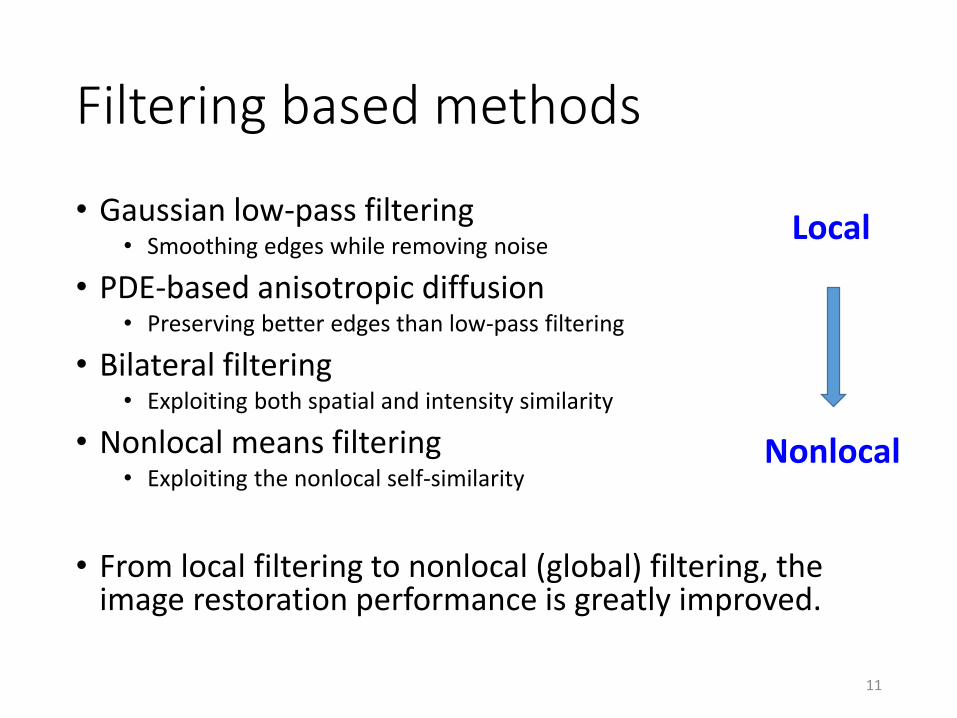
Filtering based methods

• Gaussian low-pass filtering• Smoothing edges while removing noise

• PDE-based anisotropic diffusion• Preserving better edges than low-pass filtering

• Bilateral filtering• Exploiting both spatial and intensity similarity

• Nonlocal means filtering• Exploiting the nonlocal self-similarity

• From local filtering to nonlocal (global) filtering, the image restoration performance is greatly improved.

11

Local

Nonlocal

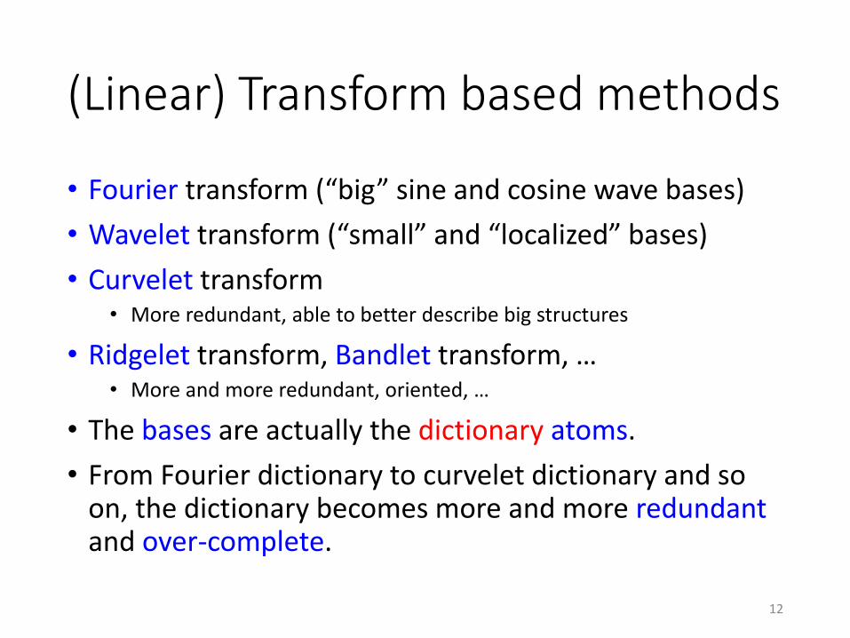
(Linear) Transform based methods

• Fourier transform (“big” sine and cosine wave bases)

• Wavelet transform (“small” and “localized” bases)

• Curvelet transform • More redundant, able to better describe big structures

• Ridgelet transform, Bandlet transform, …• More and more redundant, oriented, …

• The bases are actually the dictionary atoms.

• From Fourier dictionary to curvelet dictionary and so on, the dictionary becomes more and more redundantand over-complete.

12

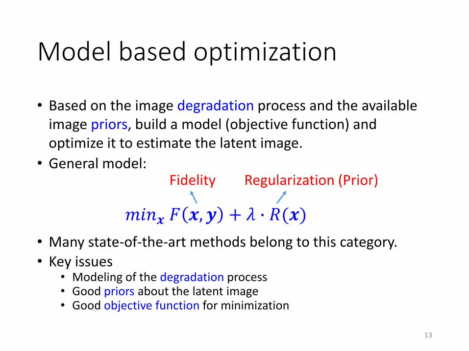
Model based optimization

• Based on the image degradation process and the available image priors, build a model (objective function) and optimize it to estimate the latent image.

• General model:

• Many state-of-the-art methods belong to this category.

• Key issues • Modeling of the degradation process • Good priors about the latent image• Good objective function for minimization

13

𝑚𝑖𝑛𝒙 𝐹 𝒙, 𝒚 + 𝜆 ∙ 𝑅(𝒙)

Fidelity Regularization (Prior)

Sparse representation for image restoration

14

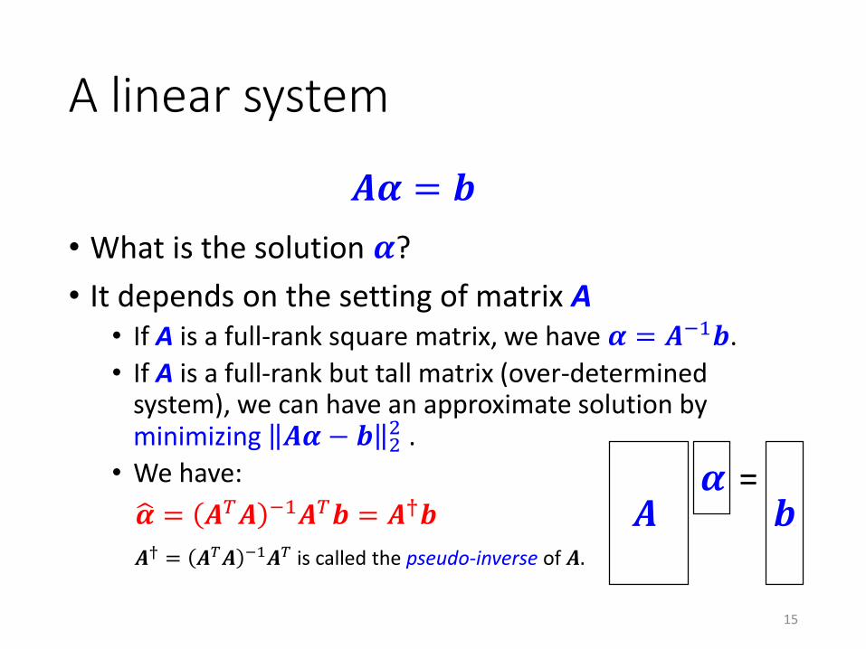
A linear system

• What is the solution 𝜶?

• It depends on the setting of matrix A• If A is a full-rank square matrix, we have 𝜶 = 𝑨−1𝒃.

• If A is a full-rank but tall matrix (over-determined system), we can have an approximate solution by minimizing 𝑨𝜶 − 𝒃 2

2 .

• We have:

𝑨𝜶 = 𝒃

𝑨=𝒃

𝜶ෝ𝜶 = 𝑨𝑇𝑨 −1𝑨𝑇𝒃 = 𝑨†𝒃

𝑨† = 𝑨𝑇𝑨 −1𝑨𝑇 is called the pseudo-inverse of 𝑨.

15

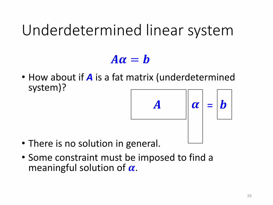
Underdetermined linear system

• How about if A is a fat matrix (underdetermined system)?

• There is no solution in general.

• Some constraint must be imposed to find a meaningful solution of 𝜶.

𝑨𝜶 = 𝒃

𝑨 = 𝒃𝜶

16

Solution

• Different objective functions 𝐽(𝜶) lead to different solutions to the underdetermined system.

• A dense solution: 𝐽 𝜶 = 𝜶 22

𝑚𝑖𝑛𝜶 𝐽 𝜶 𝑠. 𝑡. 𝑨𝜶 = 𝒃

??

.

.

.

??

A dense solution

17

Sparse solution

• The dense solution may not be useful or effective enough (e.g., not robust, not unique).

• In many applications, we may need a “sparse” solution that has many zero or nearly zero entries (e.g., more robust, more unique).

• So how to achieve this goal?

18

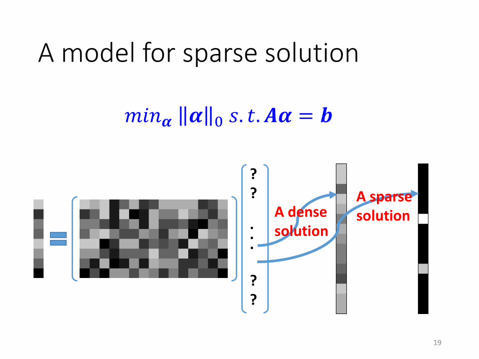
A model for sparse solution

??

.

.

.

??

A dense solution

A sparse solution

𝑚𝑖𝑛𝜶 𝜶 0 𝑠. 𝑡. 𝑨𝜶 = 𝒃

19

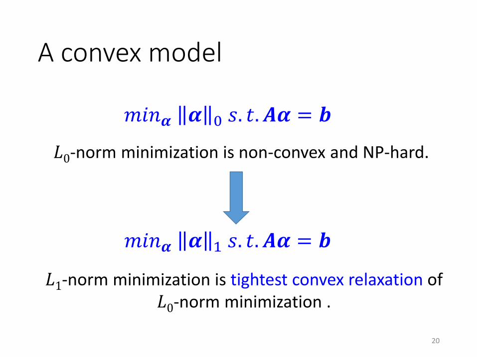
A convex model

𝑚𝑖𝑛𝜶 𝜶 0 𝑠. 𝑡. 𝑨𝜶 = 𝒃

𝐿0-norm minimization is non-convex and NP-hard.

𝐿1-norm minimization is tightest convex relaxation of 𝐿0-norm minimization .

𝑚𝑖𝑛𝜶 𝜶 1 𝑠. 𝑡. 𝑨𝜶 = 𝒃

20

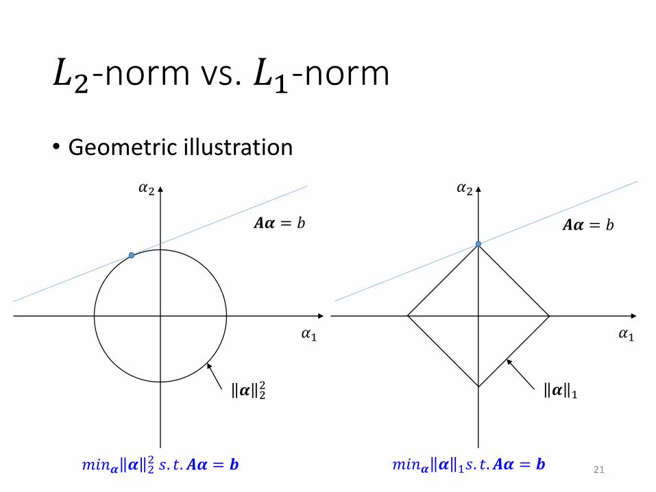
𝐿2-norm vs. 𝐿1-norm

• Geometric illustration

𝛼1

𝛼2

𝜶 22

𝑨𝜶 = 𝑏

𝑚𝑖𝑛𝜶 𝜶 22 𝑠. 𝑡. 𝑨𝜶 = 𝒃 𝑚𝑖𝑛𝜶 𝜶 1𝑠. 𝑡. 𝑨𝜶 = 𝒃

𝛼1

𝛼2

𝜶 1

𝑨𝜶 = 𝑏

21

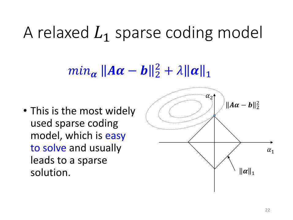
A relaxed 𝐿1 sparse coding model

• This is the most widely used sparse coding model, which is easyto solve and usually leads to a sparse solution.

𝑚𝑖𝑛𝜶 𝑨𝜶 − 𝒃 22 + 𝜆 𝜶 1

𝛼1

𝛼2

𝜶 1

𝑨𝜶 − 𝒃 22

22

Sparse coding solvers

• Greedy Search for 𝐿0-norm minimization• Matching pursuit (MP)

• Orthogonal matching pursuit (OMP)

• Convex Optimization for 𝐿1-norm minimization• Linear programming

• Iteratively reweighted least squares

• Proximal gradient descent (Iterative soft-thresholding)

• Augmented Lagrangian methods (Alternating direction method of multipliers)

23

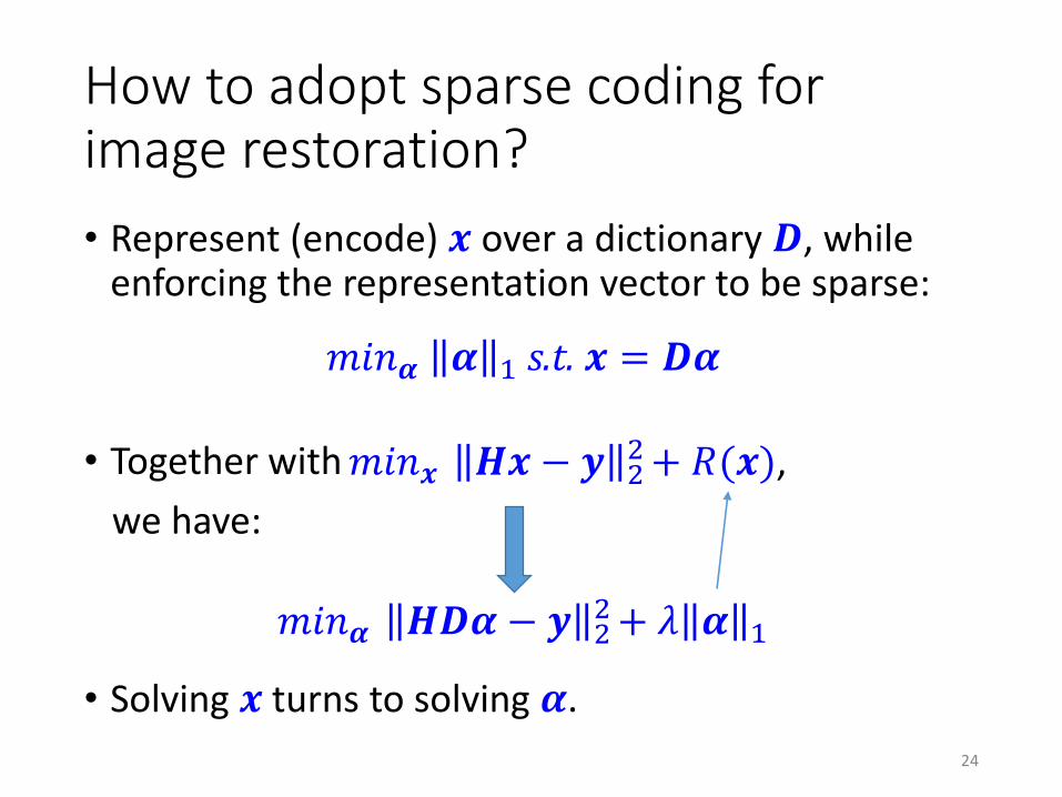
How to adopt sparse coding for image restoration?

• Represent (encode) 𝒙 over a dictionary 𝑫, while enforcing the representation vector to be sparse:

• Together with

we have:

• Solving 𝒙 turns to solving 𝜶.

𝑚𝑖𝑛𝜶 𝜶 1 s.t. 𝒙 = 𝑫𝜶

𝑚𝑖𝑛𝜶 𝑯𝑫𝜶 − 𝒚 22+ 𝜆 𝜶 1

𝑚𝑖𝑛𝒙 𝑯𝒙 − 𝒚 22+ 𝑅(𝒙),

24

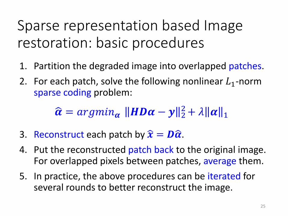
Sparse representation based Image restoration: basic procedures

1. Partition the degraded image into overlapped patches.

2. For each patch, solve the following nonlinear 𝐿1-norm sparse coding problem:

3. Reconstruct each patch by ෝ𝒙 = 𝑫ෝ𝜶.

4. Put the reconstructed patch back to the original image. For overlapped pixels between patches, average them.

5. In practice, the above procedures can be iterated for several rounds to better reconstruct the image.

25

ෝ𝜶 = 𝑎𝑟𝑔𝑚𝑖𝑛𝜶 𝑯𝑫𝜶 − 𝒚 22+ 𝜆 𝜶 1

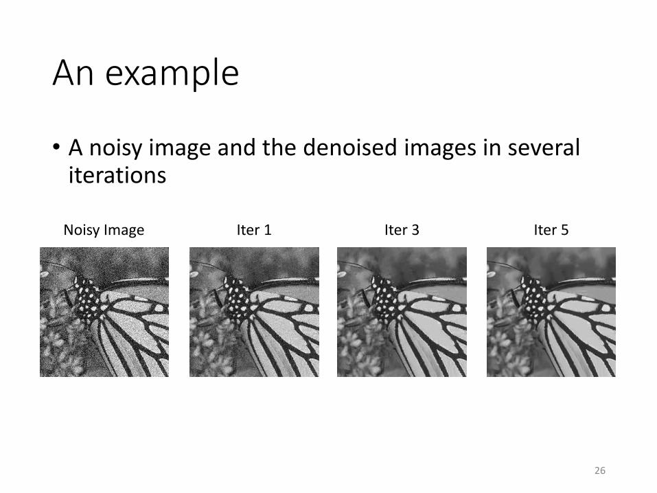
An example

• A noisy image and the denoised images in several iterations

26

Noisy Image Iter 1 Iter 3 Iter 5

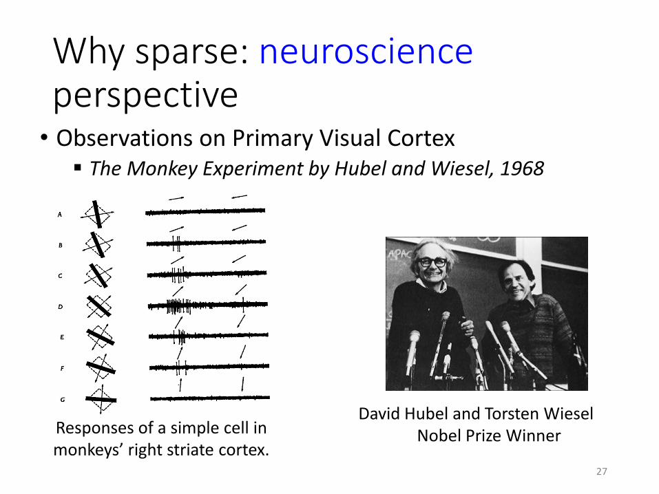
Why sparse: neuroscienceperspective

• Observations on Primary Visual Cortex The Monkey Experiment by Hubel and Wiesel, 1968

Responses of a simple cell in monkeys’ right striate cortex.

David Hubel and Torsten WieselNobel Prize Winner

27

Why sparse: neuroscienceperspective

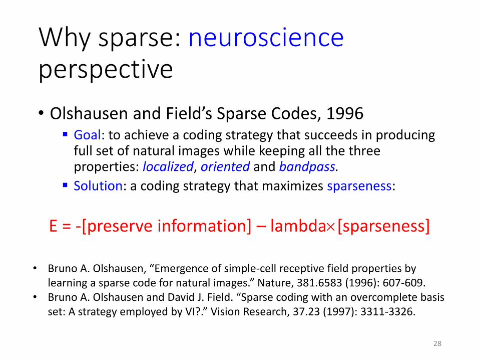
• Olshausen and Field’s Sparse Codes, 1996 Goal: to achieve a coding strategy that succeeds in producing

full set of natural images while keeping all the three properties: localized, oriented and bandpass.

Solution: a coding strategy that maximizes sparseness:

E = -[preserve information] – lambda[sparseness]

• Bruno A. Olshausen, “Emergence of simple-cell receptive field properties by learning a sparse code for natural images.” Nature, 381.6583 (1996): 607-609.

• Bruno A. Olshausen and David J. Field. “Sparse coding with an overcomplete basis set: A strategy employed by VI?.” Vision Research, 37.23 (1997): 3311-3326.

28

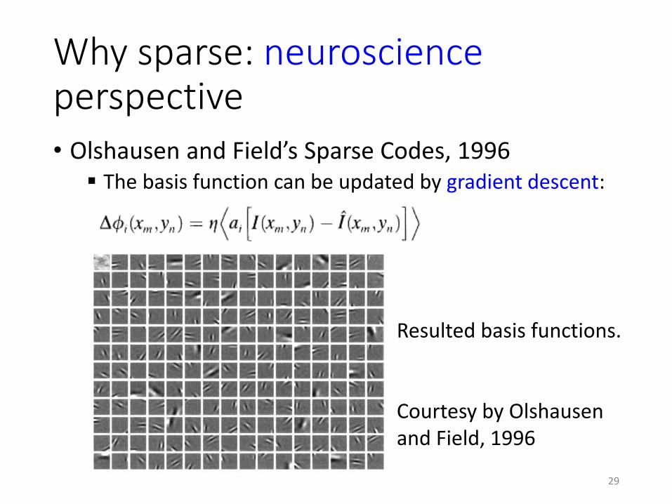
Why sparse: neuroscienceperspective• Olshausen and Field’s Sparse Codes, 1996

The basis function can be updated by gradient descent:

Resulted basis functions.

Courtesy by Olshausenand Field, 1996

29

Why sparse: Bayesian perspective

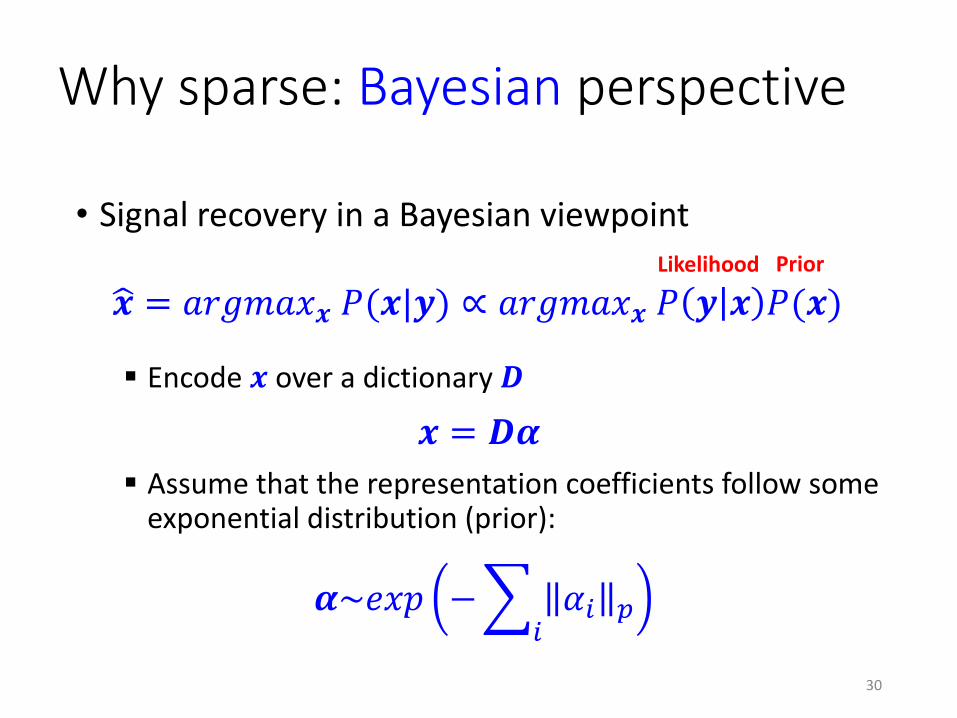
• Signal recovery in a Bayesian viewpoint

Encode 𝒙 over a dictionary 𝑫

Assume that the representation coefficients follow some exponential distribution (prior):

Likelihood Prior

30

ෝ𝒙 = 𝑎𝑟𝑔𝑚𝑎𝑥𝒙 𝑃(𝒙|𝒚) ∝ 𝑎𝑟𝑔𝑚𝑎𝑥𝒙 𝑃 𝒚 𝒙 𝑃(𝒙)

𝒙 = 𝑫𝜶

𝜶~𝑒𝑥𝑝 −𝑖𝛼𝑖 𝑝

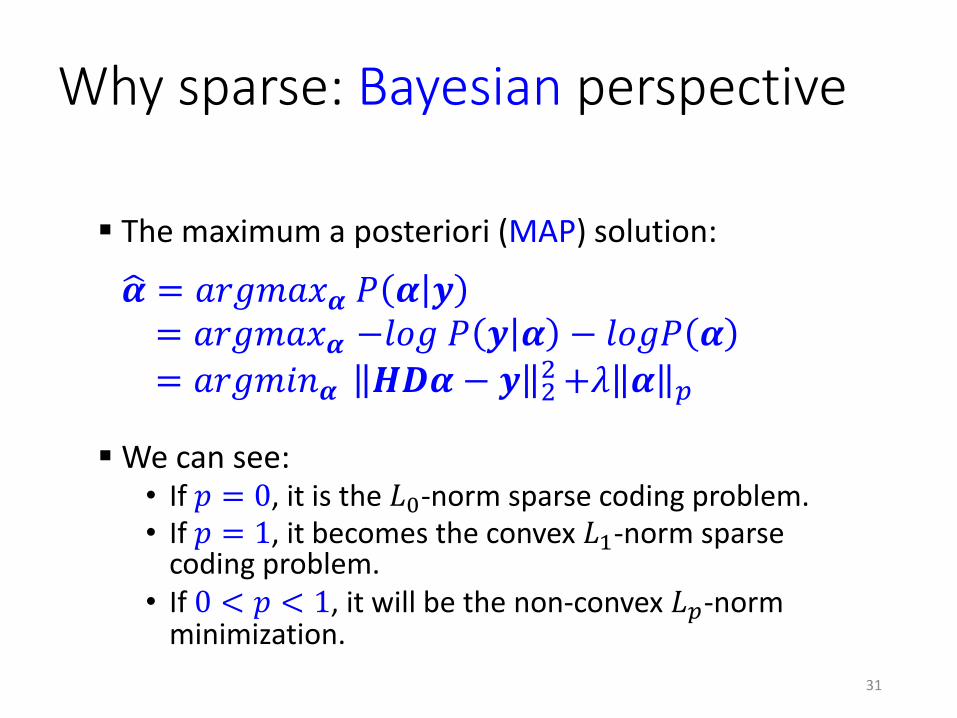
The maximum a posteriori (MAP) solution:

We can see:• If 𝑝 = 0, it is the 𝐿0-norm sparse coding problem.• If 𝑝 = 1, it becomes the convex 𝐿1-norm sparse

coding problem.• If 0 < 𝑝 < 1, it will be the non-convex 𝐿𝑝-norm

minimization.

Why sparse: Bayesian perspective

31

ෝ𝜶 = 𝑎𝑟𝑔𝑚𝑎𝑥𝜶 𝑃 𝜶 𝒚= 𝑎𝑟𝑔𝑚𝑎𝑥𝜶 −𝑙𝑜𝑔 𝑃 𝒚 𝜶 − 𝑙𝑜𝑔𝑃 𝜶

= 𝑎𝑟𝑔𝑚𝑖𝑛𝜶 𝑯𝑫𝜶 − 𝒚 22+𝜆 𝜶 𝑝

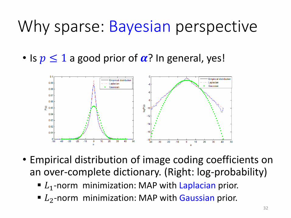
• Is 𝑝 ≤ 1 a good prior of 𝜶? In general, yes!

• Empirical distribution of image coding coefficients on an over-complete dictionary. (Right: log-probability) 𝐿1-norm minimization: MAP with Laplacian prior.

𝐿2-norm minimization: MAP with Gaussian prior.

Why sparse: Bayesian perspective

32

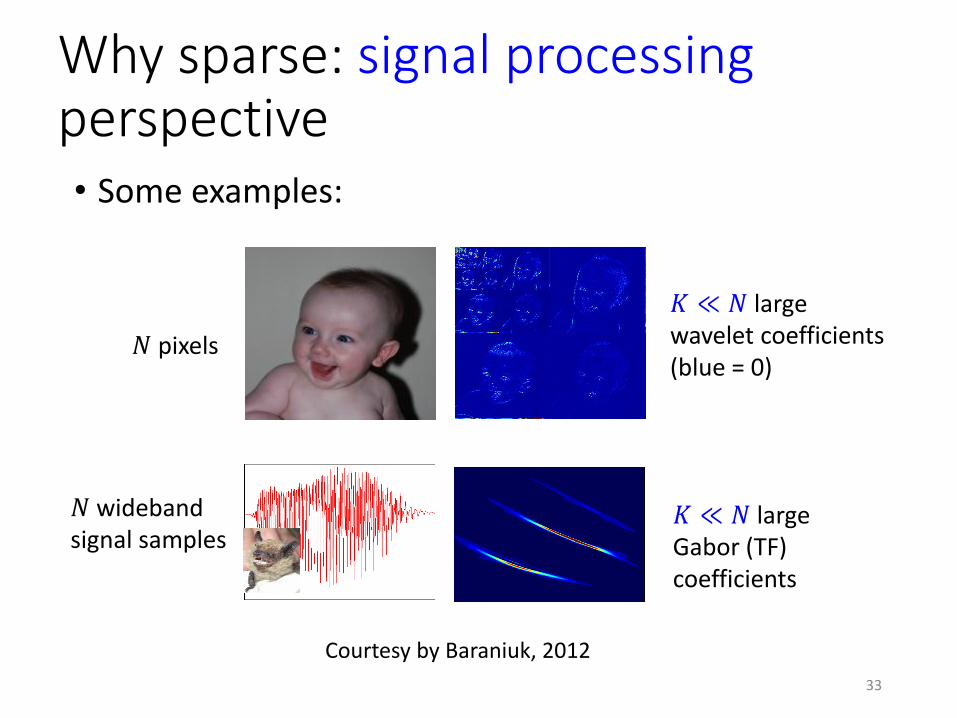
• Some examples:

𝑁 pixels

𝐾 ≪ 𝑁 largewavelet coefficients(blue = 0)

𝑁 widebandsignal samples

𝐾 ≪ 𝑁 largeGabor (TF)coefficients

Courtesy by Baraniuk, 2012

Why sparse: signal processing perspective

33

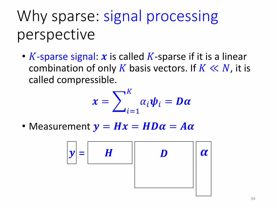
• 𝐾-sparse signal: 𝒙 is called 𝐾-sparse if it is a linear combination of only 𝐾 basis vectors. If 𝐾 ≪ 𝑁, it is called compressible.

• Measurement 𝒚 = 𝑯𝒙 = 𝑯𝑫𝜶 = 𝑨𝜶

34

Why sparse: signal processing perspective

𝒙 =𝑖=1

𝐾

𝛼𝑖𝝍𝑖 = 𝑫𝜶

𝑯= 𝜶𝑫𝒚

Why sparse: signal processing perspective

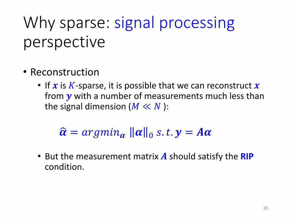
• Reconstruction• If 𝒙 is 𝐾-sparse, it is possible that we can reconstruct 𝒙

from 𝒚 with a number of measurements much less than the signal dimension (𝑀 ≪ 𝑁 ):

• But the measurement matrix 𝑨 should satisfy the RIPcondition.

35

ෝ𝜶 = 𝑎𝑟𝑔𝑚𝑖𝑛𝜶 𝜶 0 𝑠. 𝑡. 𝒚 = 𝑨𝜶

Why sparsity helps signal recovery?An illustrative example

• You are looking for your another half.• i.e., you are “reconstructing” the desired signal.

• You hope that she/he is “白-富-美”/ “高-富-帅”.• i.e., you want a “clean” and “perfect” reconstruction.

• However, there are limited candidates.• i.e., the dictionary is small. (For example, your search

space is constrained to a class in PolyU.)

• Can you easily find your ideal another half?36

Why sparsity helps signal recovery?A illustrative example

• Candidate A is tall; however, he is too poor.

• Candidate B is rich; however, he is too fat.

• Candidate C is handsome; however, he is not healthy.

• If you sparsely select one of them, none is ideal for you• i.e., a sparse representation vector such as [0, 1, 0].

• How about a dense solution: (A+B+C)/3?• i.e., a dense representation vector [1, 1, 1]/3

• The “reconstructed one” is somewhat “高-富-帅”, but he is fat and unhealthy (i.e., noise) at the same time.

37

Why sparsity helps signal recovery?A illustrative example

• So what’s the problem?• This is because the dictionary is too small!

• If you are able to find your another half from all candidates all over the world (i.e., a large enough dictionary) , there is a very high probability (nearly 1) that you will find the one.• i.e., a very sparse solution [0, …, 1, …, 0].

• In summary, a sparse solution with an over-complete dictionary often works!

• Sparsity (coefficients) and redundancy (dictionary) are the two sides of the same coin.

38

Dictionary

• Analytical dictionaries• DCT bases• Wavelets• Curvelets• Ridgelets, bandlets, …

• Learn dictionaries from natural images• K-SVD• Coordinate descent • Multi-scale dictionary learning• Adaptive PCA dictionaries• …

39

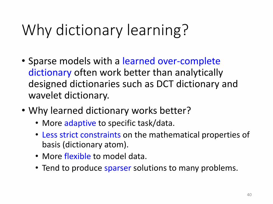
Why dictionary learning?

• Sparse models with a learned over-complete dictionary often work better than analytically designed dictionaries such as DCT dictionary and wavelet dictionary.

• Why learned dictionary works better?• More adaptive to specific task/data.

• Less strict constraints on the mathematical properties of basis (dictionary atom).

• More flexible to model data.

• Tend to produce sparser solutions to many problems.

40

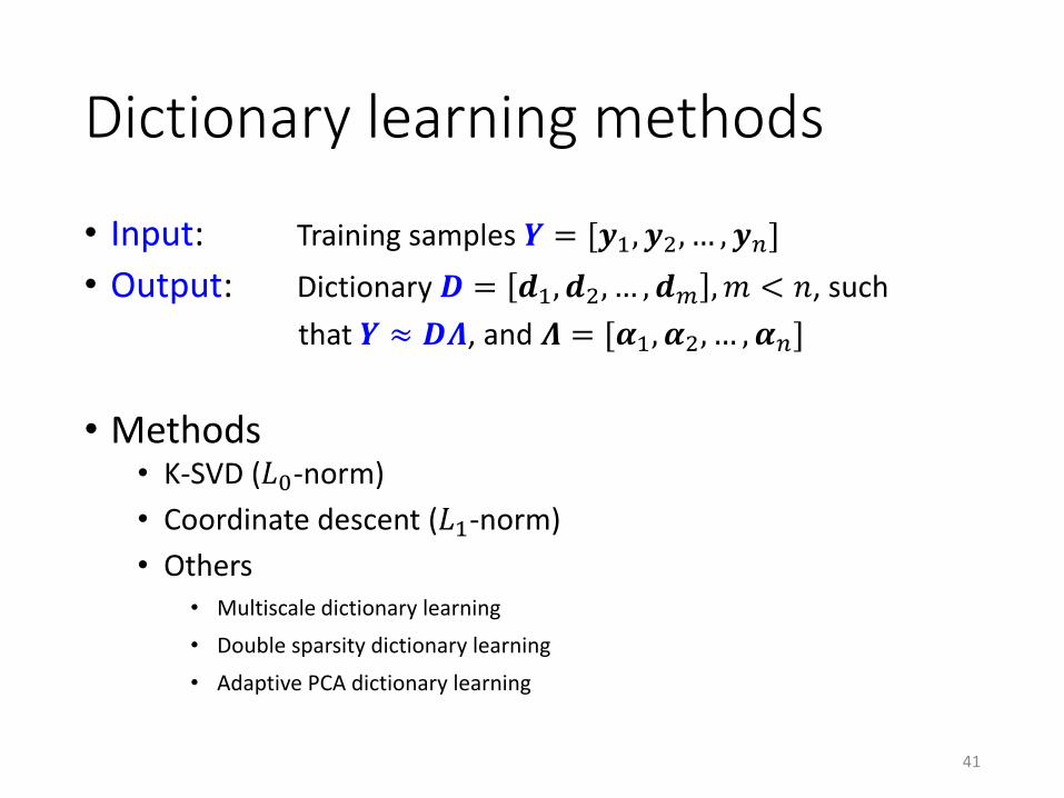
Dictionary learning methods

• Input: Training samples 𝒀 = [𝒚1, 𝒚2, … , 𝒚𝑛]

• Output: Dictionary 𝑫 = 𝒅1, 𝒅2, … , 𝒅𝑚 , 𝑚 < 𝑛, such

that 𝒀 ≈ 𝑫𝜦, and 𝜦 = [𝜶1, 𝜶2, … , 𝜶𝑛]

• Methods• K-SVD (𝐿0-norm)

• Coordinate descent (𝐿1-norm)

• Others• Multiscale dictionary learning

• Double sparsity dictionary learning

• Adaptive PCA dictionary learning

41

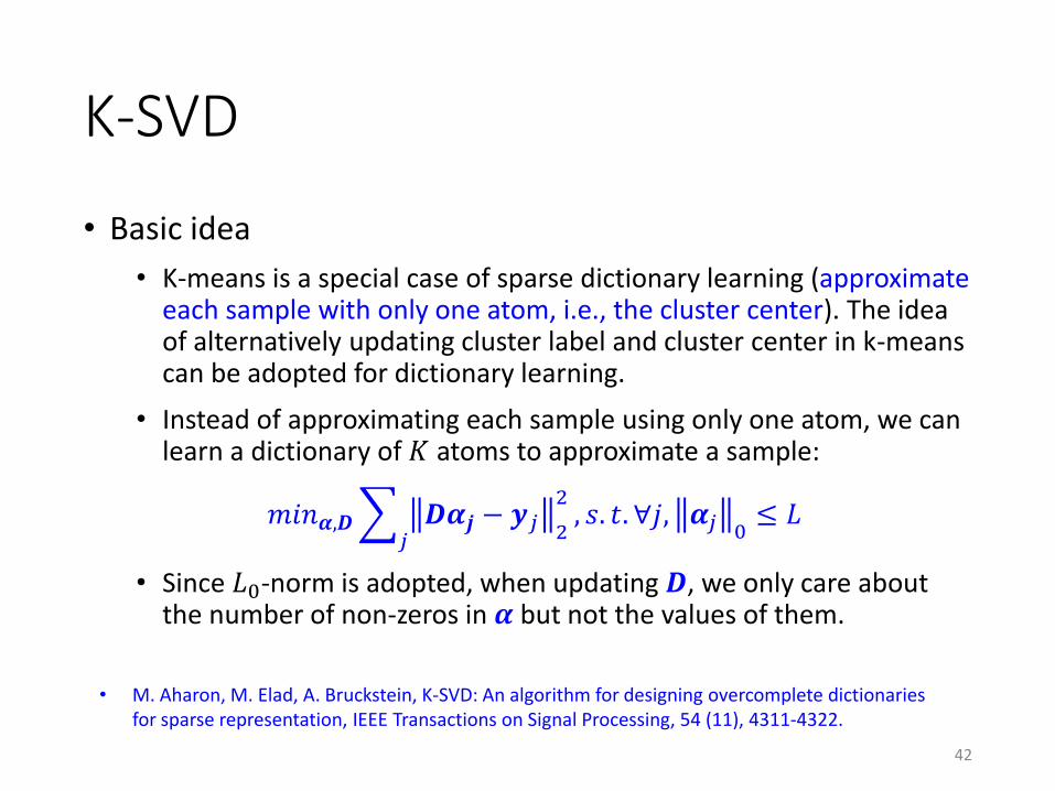
K-SVD

• Basic idea

• K-means is a special case of sparse dictionary learning (approximate each sample with only one atom, i.e., the cluster center). The idea of alternatively updating cluster label and cluster center in k-means can be adopted for dictionary learning.

• Instead of approximating each sample using only one atom, we can learn a dictionary of 𝐾 atoms to approximate a sample:

• Since 𝐿0-norm is adopted, when updating 𝑫, we only care about the number of non-zeros in 𝜶 but not the values of them.

42

𝑚𝑖𝑛𝜶,𝑫𝑗𝑫𝜶𝒋 − 𝒚𝑗 2

2, 𝑠. 𝑡. ∀𝑗, 𝜶𝑗 0

≤ 𝐿

• M. Aharon, M. Elad, A. Bruckstein, K-SVD: An algorithm for designing overcomplete dictionaries for sparse representation, IEEE Transactions on Signal Processing, 54 (11), 4311-4322.

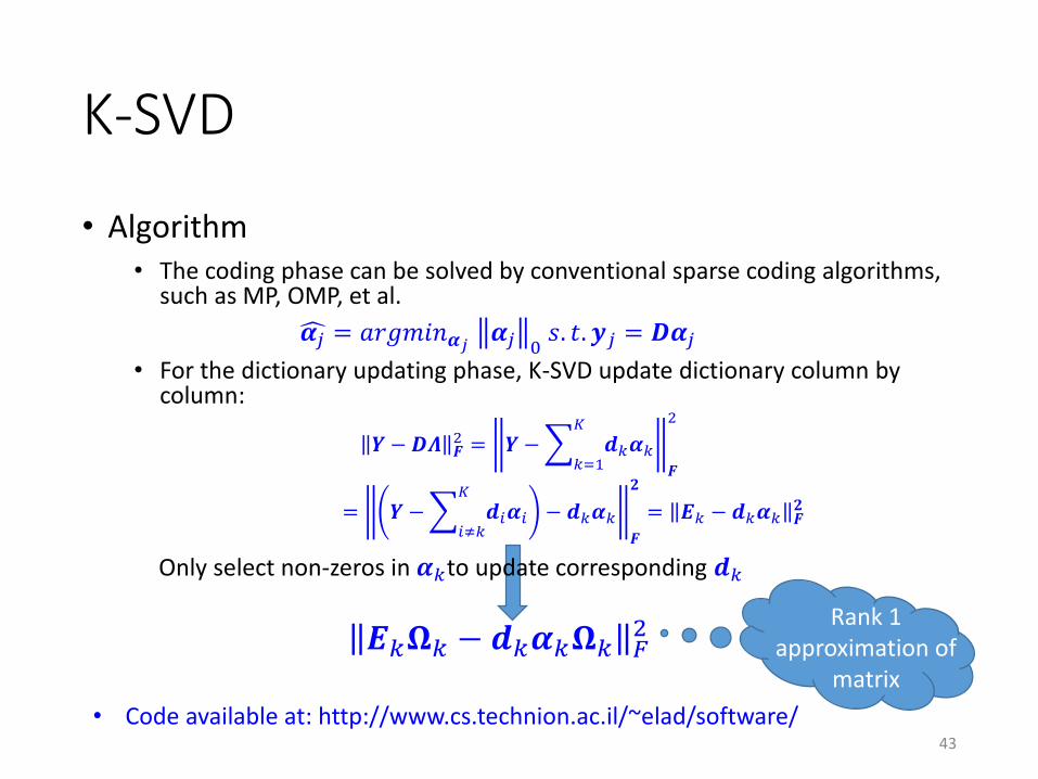
K-SVD

• Algorithm• The coding phase can be solved by conventional sparse coding algorithms,

such as MP, OMP, et al.

• For the dictionary updating phase, K-SVD update dictionary column by column:

𝒀 − 𝑫𝜦 𝑭2 = 𝒀 −

𝑘=1

𝐾

𝒅𝑘𝜶𝑘𝑭

2

= 𝒀 −𝑖≠𝑘

𝐾

𝒅𝑖𝜶𝑖 − 𝒅𝑘𝜶𝑘𝑭

𝟐

= 𝑬𝑘 − 𝒅𝑘𝜶𝑘 𝑭𝟐

43

Only select non-zeros in 𝜶𝑘to update corresponding 𝒅𝑘

Rank 1 approximation of

matrix

• Code available at: http://www.cs.technion.ac.il/~elad/software/

ෞ𝜶𝑗 = 𝑎𝑟𝑔𝑚𝑖𝑛𝜶𝑗 𝜶𝑗 0𝑠. 𝑡. 𝒚𝑗 = 𝑫𝜶𝑗

𝑬𝑘𝛀𝑘 − 𝒅𝑘𝜶𝑘𝛀𝑘 𝐹2

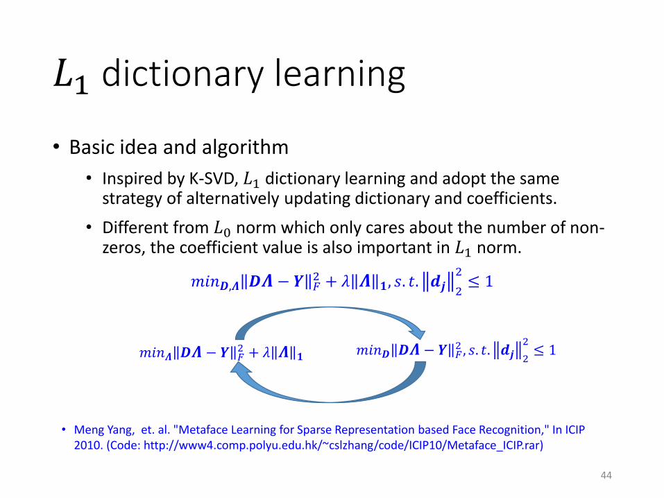
𝐿1 dictionary learning

• Basic idea and algorithm

• Inspired by K-SVD, 𝐿1 dictionary learning and adopt the same strategy of alternatively updating dictionary and coefficients.

• Different from 𝐿0 norm which only cares about the number of non-zeros, the coefficient value is also important in 𝐿1 norm.

44

𝑚𝑖𝑛𝑫,𝜦 𝑫𝜦 − 𝒀 𝐹2 + 𝜆 𝜦 𝟏, 𝑠. 𝑡. 𝒅𝒋 2

2≤ 1

• Meng Yang, et. al. "Metaface Learning for Sparse Representation based Face Recognition," In ICIP 2010. (Code: http://www4.comp.polyu.edu.hk/~cslzhang/code/ICIP10/Metaface_ICIP.rar)

𝑚𝑖𝑛𝜦 𝑫𝜦 − 𝒀 𝐹2 + 𝜆 𝜦 𝟏

𝑚𝑖𝑛𝑫 𝑫𝜦 − 𝒀 𝐹2 , 𝑠. 𝑡. 𝒅𝒋 2

2≤ 1

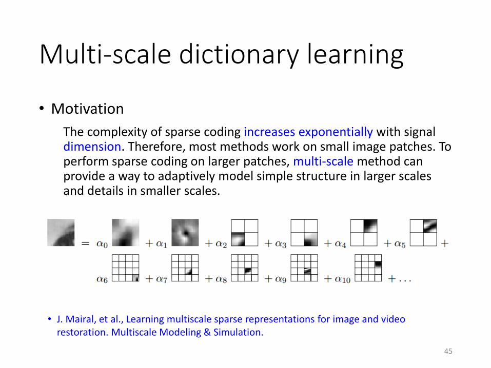
Multi-scale dictionary learning

• Motivation

The complexity of sparse coding increases exponentially with signal dimension. Therefore, most methods work on small image patches. To perform sparse coding on larger patches, multi-scale method can provide a way to adaptively model simple structure in larger scales and details in smaller scales.

45

• J. Mairal, et al., Learning multiscale sparse representations for image and video restoration. Multiscale Modeling & Simulation.

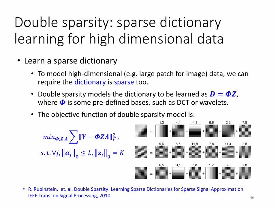
Double sparsity: sparse dictionary learning for high dimensional data

• Learn a sparse dictionary

• To model high-dimensional (e.g. large patch for image) data, we can require the dictionary is sparse too.

• Double sparsity models the dictionary to be learned as 𝑫 = 𝜱𝒁, where 𝜱 is some pre-defined bases, such as DCT or wavelets.

• The objective function of double sparsity model is:

46

• R. Rubinstein, et. al. Double Sparsity: Learning Sparse Dictionaries for Sparse Signal Approximation. IEEE Trans. on Signal Processing, 2010.

𝑚𝑖𝑛𝜱,𝒁,𝜦 𝒀−𝜱𝒁𝜦 𝐹2 ,

𝑠. 𝑡. ∀𝑗, 𝜶𝑗 0≤ 𝐿, 𝒛𝑗 0

= 𝐾

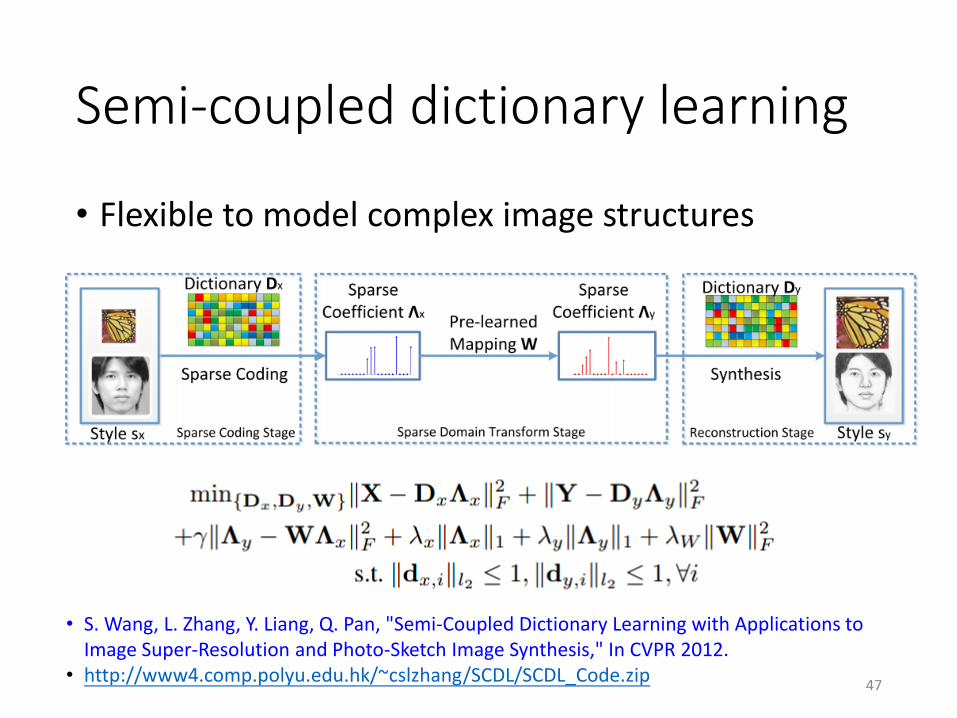
Semi-coupled dictionary learning

• Flexible to model complex image structures

47

• S. Wang, L. Zhang, Y. Liang, Q. Pan, "Semi-Coupled Dictionary Learning with Applications to Image Super-Resolution and Photo-Sketch Image Synthesis," In CVPR 2012.

• http://www4.comp.polyu.edu.hk/~cslzhang/SCDL/SCDL_Code.zip

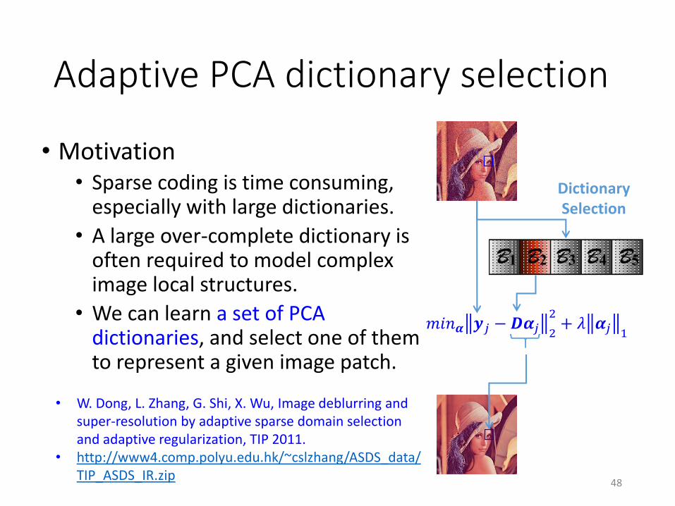
Adaptive PCA dictionary selection

• Motivation• Sparse coding is time consuming,

especially with large dictionaries.

• A large over-complete dictionary is often required to model complex image local structures.

• We can learn a set of PCA dictionaries, and select one of them to represent a given image patch.

48

Dictionary Selection

𝑚𝑖𝑛𝜶 𝒚𝑗 − 𝑫𝜶𝑗 2

2+ 𝜆 𝜶𝑗 1

• W. Dong, L. Zhang, G. Shi, X. Wu, Image deblurring and super-resolution by adaptive sparse domain selection and adaptive regularization, TIP 2011.

• http://www4.comp.polyu.edu.hk/~cslzhang/ASDS_data/TIP_ASDS_IR.zip

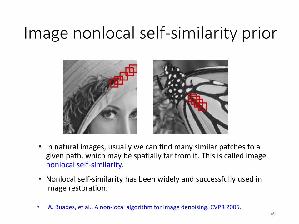
Image nonlocal self-similarity prior

• In natural images, usually we can find many similar patches to a given path, which may be spatially far from it. This is called image nonlocal self-similarity.

• Nonlocal self-similarity has been widely and successfully used in image restoration.

49• A. Buades, et al., A non-local algorithm for image denoising. CVPR 2005.

Non-locally centralized sparse representation (NCSR)

• A neat but very effective sparse representation model, which naturally integrates nonlocal self-similarity (NSS) prior and sparse coding.

W. Dong, L. Zhang and G. Shi, “Centralized Sparse Representation for Image Restoration”, in ICCV 2011.

W. Dong, L. Zhang, G. Shi and X. Li, “Nonlocally Centralized Sparse Representation for Image Restoration”, IEEE Trans. on Image Processing, vol. 22, no. 4, pp. 1620-1630, April 2013.

http://www4.comp.polyu.edu.hk/~cslzhang/code/NCSR.rar

50

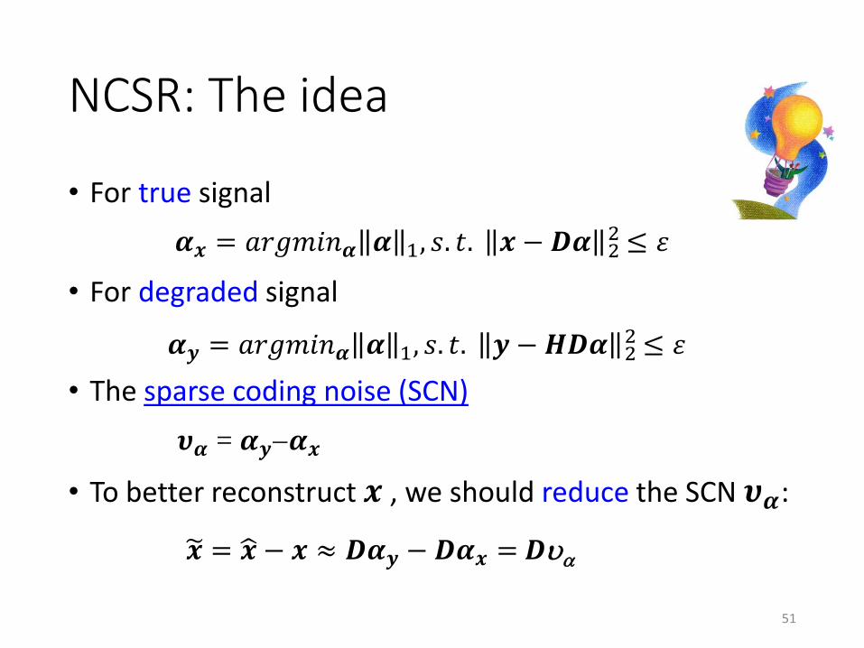
NCSR: The idea

• For true signal

• For degraded signal

• The sparse coding noise (SCN)

• To better reconstruct 𝒙 , we should reduce the SCN 𝝊𝜶:

51

𝝊𝜶 = 𝜶𝒚𝜶𝒙

𝜶𝒙 = 𝑎𝑟𝑔𝑚𝑖𝑛𝜶 𝜶 1, 𝑠. 𝑡. 𝒙 − 𝑫𝜶 22≤ 𝜀

𝜶𝒚 = 𝑎𝑟𝑔𝑚𝑖𝑛𝜶 𝜶 1, 𝑠. 𝑡. 𝒚 − 𝑯𝑫𝜶 22≤ 𝜀

𝒙 = ෝ𝒙 − 𝒙 ≈ 𝑫𝜶𝒚 −𝑫𝜶𝒙 =𝑫

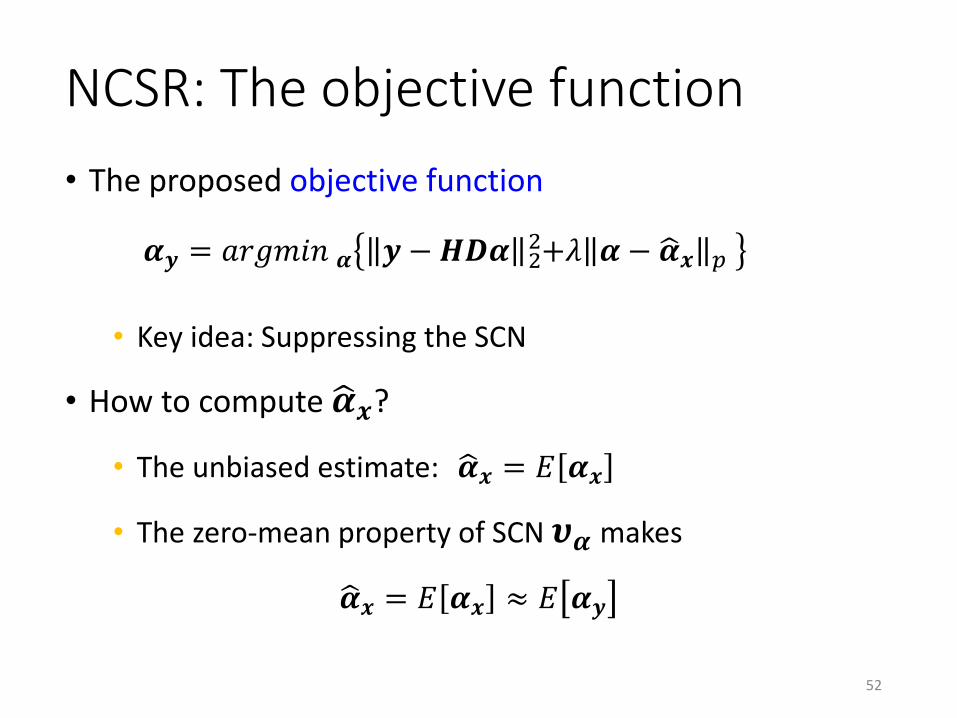
NCSR: The objective function

• The proposed objective function

• Key idea: Suppressing the SCN

• How to compute ෝ𝜶𝒙?

• The unbiased estimate:

• The zero-mean property of SCN 𝝊𝜶 makes

52

𝜶𝒚 = 𝑎𝑟𝑔𝑚𝑖𝑛 𝜶 𝒚 −𝑯𝑫𝜶 22+𝜆 𝜶 − ෝ𝜶𝒙 𝑝

ෝ𝜶𝒙 = 𝐸 𝜶𝒙

ෝ𝜶𝒙 = 𝐸 𝜶𝒙 ≈ 𝐸 𝜶𝒚

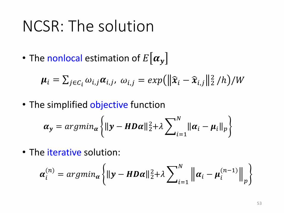
• The nonlocal estimation of 𝐸 𝜶𝒚

• The simplified objective function

• The iterative solution:

NCSR: The solution

53

𝝁𝑖 = σ𝑗∈𝐶𝑖𝜔𝑖,𝑗𝜶𝑖,𝑗, 𝜔𝑖,𝑗 = 𝑒𝑥𝑝 ෝ𝒙𝑖 − ෝ𝒙𝑖,𝑗 2

2 /ℎ /𝑊

𝜶𝒚 = 𝑎𝑟𝑔𝑚𝑖𝑛𝜶 𝒚 − 𝑯𝑫𝜶 22+𝜆

𝑖=1

𝑁

𝜶𝑖 − 𝝁𝑖 𝑝

𝜶𝑖(𝑛)

= 𝑎𝑟𝑔𝑚𝑖𝑛𝜶 𝒚 − 𝑯𝑫𝜶 22+𝜆

𝑖=1

𝑁

𝜶𝑖 − 𝝁𝑖(𝑛−1)

𝑝

• The 𝐿𝑝-norm is set to 𝐿1-norm since SCN is generally

Laplacian distributed.

• The regularization parameter 𝜆 is adaptively determined

based on the MAP estimation principle.

• Local adaptive PCA dictionaries are used, which are

learned from the given image.

Cluster the image patches, and for each cluster, a PCA

dictionary is learned and used to code the patches within

this cluster.

NSCR: The parameters and dictionaries

54

Low-rank minimization for image restoration

55

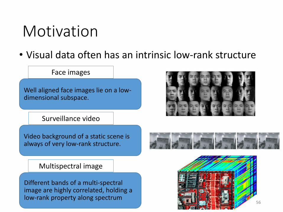
Motivation

• Visual data often has an intrinsic low-rank structure

Face images

Surveillance video

Multispectral image

Well aligned face images lie on a low-dimensional subspace.

Video background of a static scene is always of very low-rank structure.

Different bands of a multi-spectral image are highly correlated, holding a low-rank property along spectrum

56

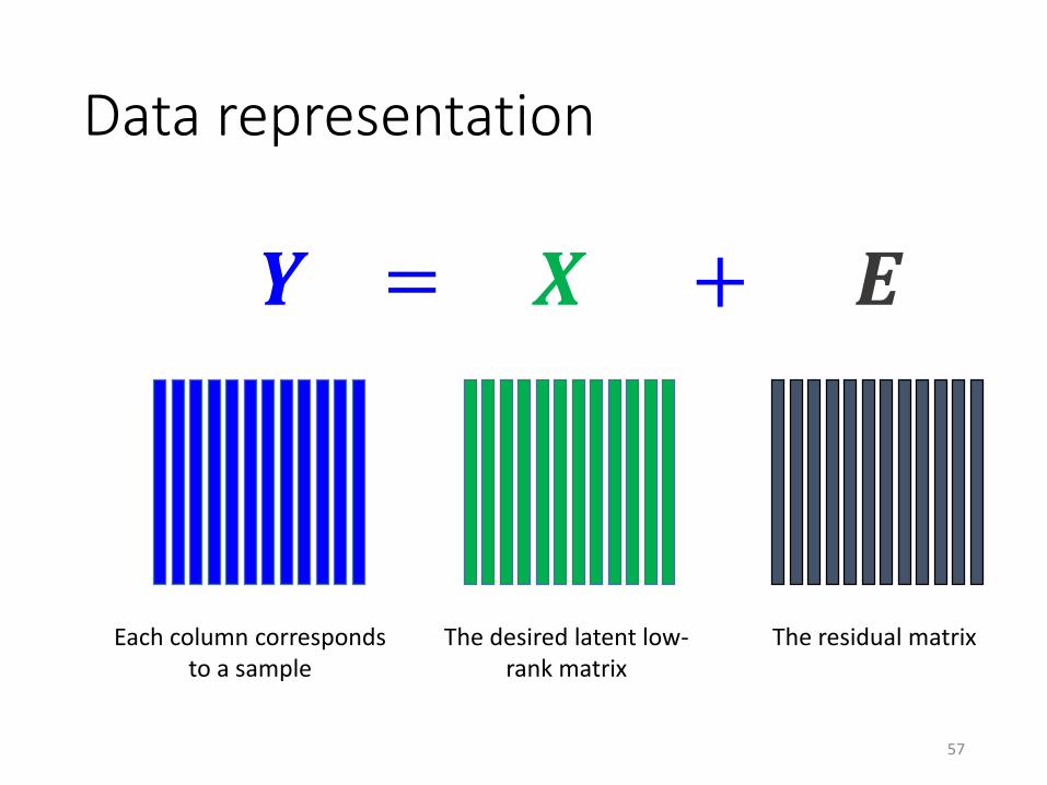
Data representation

57

Each column corresponds to a sample

𝒀 = 𝑿 + 𝑬

The desired latent low-rank matrix

The residual matrix

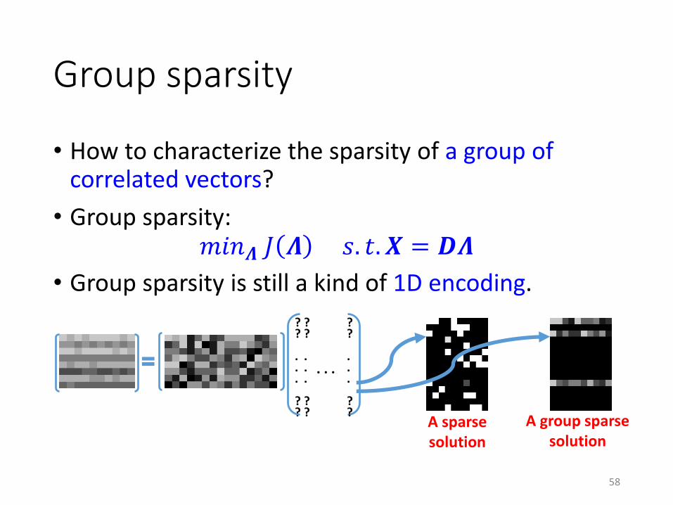
Group sparsity

• How to characterize the sparsity of a group of correlated vectors?

• Group sparsity:𝑚𝑖𝑛𝜦 𝐽 𝜦 𝑠. 𝑡. 𝑿 = 𝑫𝜦

• Group sparsity is still a kind of 1D encoding.

58

??

.

.

.

??

??

.

.

.

??

??

.

.

.

??

. . .

A sparse solution

A group sparse solution

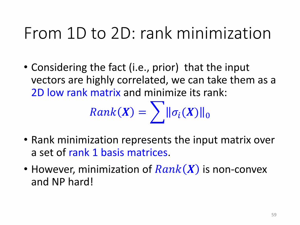
From 1D to 2D: rank minimization

59

• Considering the fact (i.e., prior) that the input vectors are highly correlated, we can take them as a 2D low rank matrix and minimize its rank:

𝑅𝑎𝑛𝑘 𝑿 = 𝜎𝑖(𝑿) 0

• Rank minimization represents the input matrix over a set of rank 1 basis matrices.

• However, minimization of 𝑅𝑎𝑛𝑘 𝑿 is non-convex and NP hard!

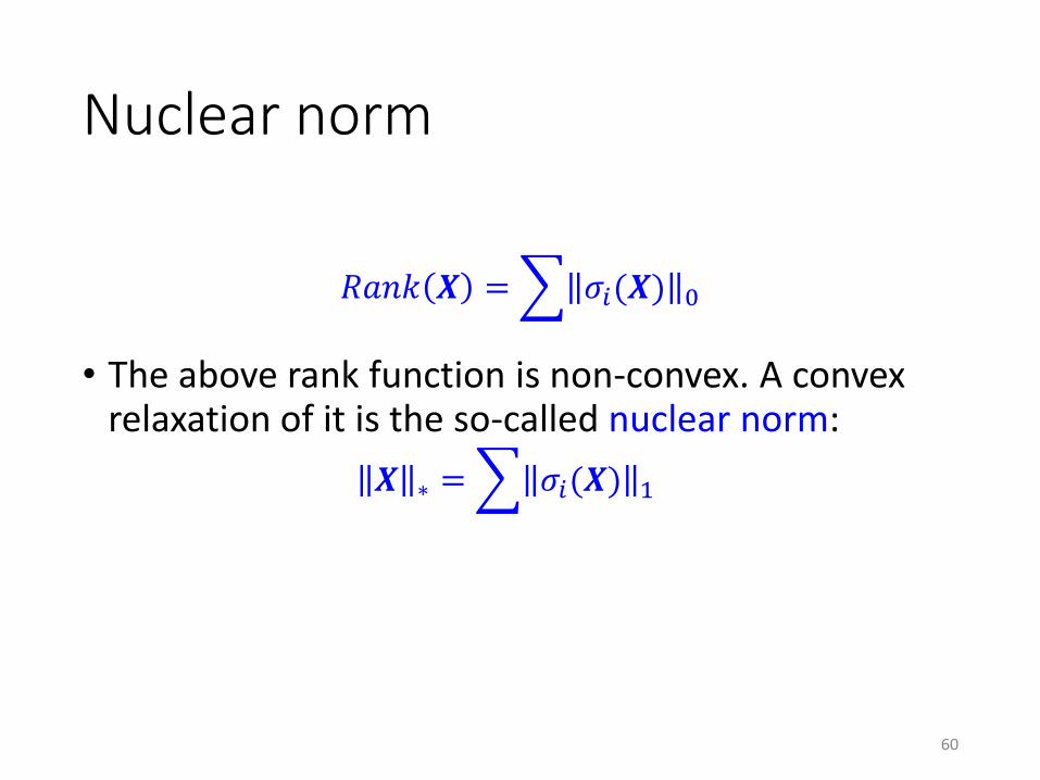
Nuclear norm

𝑅𝑎𝑛𝑘 𝑿 = 𝜎𝑖(𝑿) 0

• The above rank function is non-convex. A convex relaxation of it is the so-called nuclear norm:

𝑿 ∗ = 𝜎𝑖(𝑿) 1

60

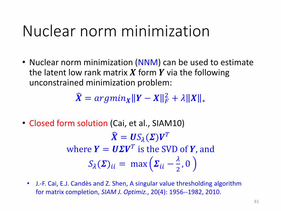
Nuclear norm minimization

61

• Nuclear norm minimization (NNM) can be used to estimate the latent low rank matrix 𝑿 form 𝒀 via the following unconstrained minimization problem:

𝑿 = 𝑎𝑟𝑔𝑚𝑖𝑛𝑿 𝒀 − 𝑿 𝐹2 + 𝜆 𝑿 ∗

• Closed form solution (Cai, et al., SIAM10)

𝑿 = 𝑼𝑆𝜆(𝜮)𝑽𝑇

where 𝒀 = 𝑼𝜮𝑽𝑇 is the SVD of 𝒀, and

𝑆𝜆(𝜮)𝑖𝑖 = max 𝜮𝑖𝑖 −𝜆

2, 0

• J.-F. Cai, E.J. Candès and Z. Shen, A singular value thresholding algorithm for matrix completion, SIAM J. Optimiz., 20(4): 1956--1982, 2010.

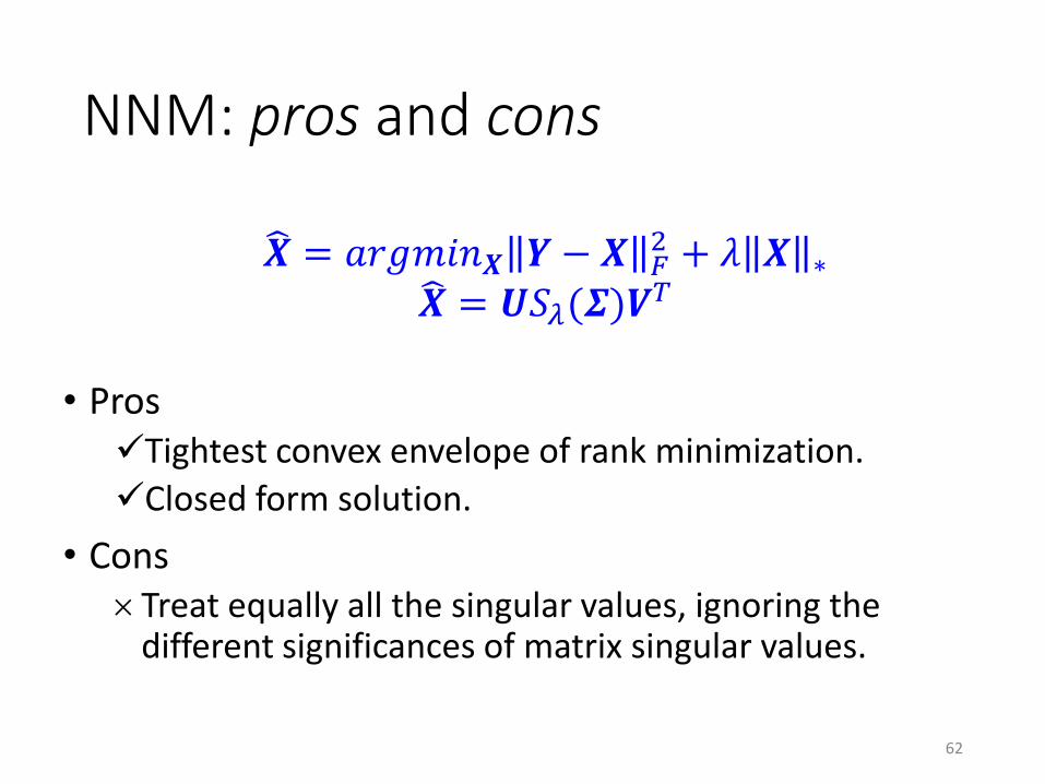
NNM: pros and cons

• ProsTightest convex envelope of rank minimization.

Closed form solution.

• ConsTreat equally all the singular values, ignoring the

different significances of matrix singular values.

62

𝑿 = 𝑎𝑟𝑔𝑚𝑖𝑛𝑿 𝒀 − 𝑿 𝐹2 + 𝜆 𝑿 ∗

𝑿 = 𝑼𝑆𝜆(𝜮)𝑽𝑇

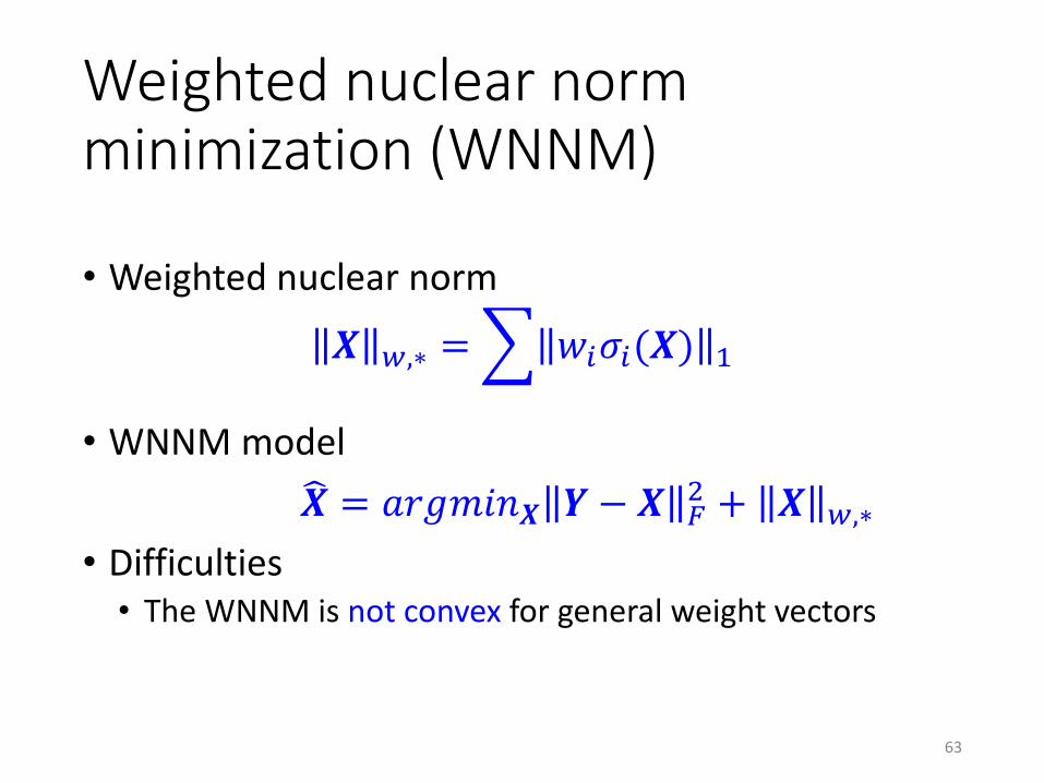
Weighted nuclear norm minimization (WNNM)

63

• Weighted nuclear norm

𝑿 𝑤,∗ = 𝑤𝑖𝜎𝑖(𝑿) 1

• WNNM model

𝑿 = 𝑎𝑟𝑔𝑚𝑖𝑛𝑿 𝒀 − 𝑿 𝐹2 + 𝑿 𝑤,∗

• Difficulties• The WNNM is not convex for general weight vectors

Optimization of WNNM

64

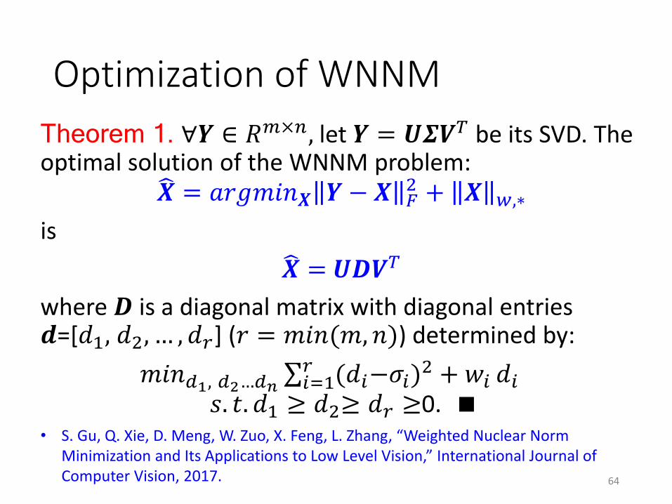
Theorem 1. ∀𝒀 ∈ 𝑅𝑚×𝑛, let 𝒀 = 𝑼𝜮𝑽𝑇 be its SVD. The optimal solution of the WNNM problem:

𝑿 = 𝑎𝑟𝑔𝑚𝑖𝑛𝑿 𝒀 − 𝑿 𝐹2 + 𝑿 𝑤,∗

is

𝑿 = 𝑼𝑫𝑽𝑇

where 𝑫 is a diagonal matrix with diagonal entries 𝒅=[𝑑1, 𝑑2, … , 𝑑𝑟] (𝑟 = 𝑚𝑖𝑛(𝑚, 𝑛)) determined by:

𝑚𝑖𝑛𝑑1, 𝑑2…𝑑𝑛 σ𝑖=1𝑟 (𝑑𝑖−𝜎𝑖)

2 + 𝑤𝑖 𝑑𝑖𝑠. 𝑡. 𝑑1 ≥ 𝑑2≥ 𝑑𝑟 ≥0.

• S. Gu, Q. Xie, D. Meng, W. Zuo, X. Feng, L. Zhang, “Weighted Nuclear Norm Minimization and Its Applications to Low Level Vision,” International Journal of Computer Vision, 2017.

An important corollary

65

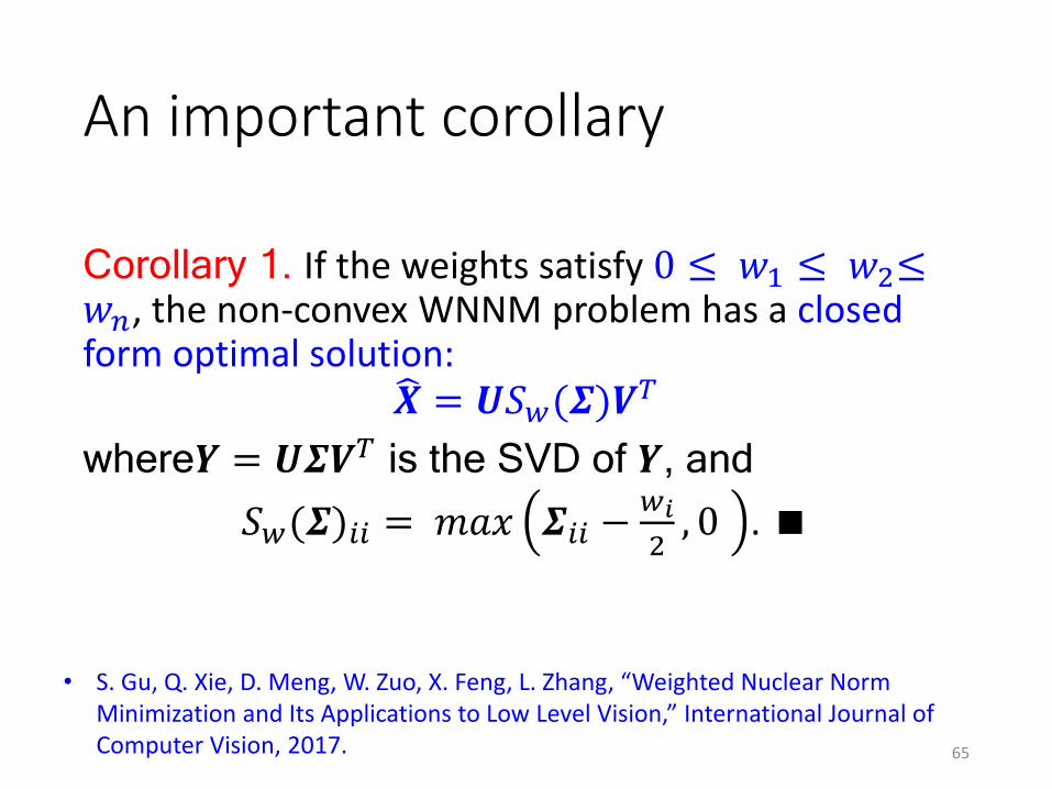
Corollary 1. If the weights satisfy 0 ≤ 𝑤1 ≤ 𝑤2≤𝑤𝑛, the non-convex WNNM problem has a closed form optimal solution:

𝑿 = 𝑼𝑆𝑤(𝜮)𝑽𝑇

where𝒀 = 𝑼𝜮𝑽𝑇 is the SVD of 𝒀, and

𝑆𝑤(𝜮)𝑖𝑖 = 𝑚𝑎𝑥 𝜮𝑖𝑖 −𝑤𝑖

2, 0 .

• S. Gu, Q. Xie, D. Meng, W. Zuo, X. Feng, L. Zhang, “Weighted Nuclear Norm Minimization and Its Applications to Low Level Vision,” International Journal of Computer Vision, 2017.

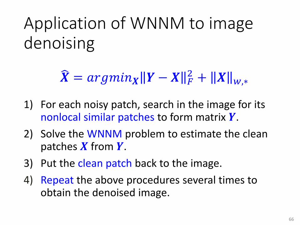
Application of WNNM to image denoising

1) For each noisy patch, search in the image for its nonlocal similar patches to form matrix 𝒀.

2) Solve the WNNM problem to estimate the clean patches 𝑿 from 𝒀.

3) Put the clean patch back to the image.

4) Repeat the above procedures several times to obtain the denoised image.

66

𝑿 = 𝑎𝑟𝑔𝑚𝑖𝑛𝑿 𝒀 − 𝑿 𝐹2 + 𝑿 𝑤,∗

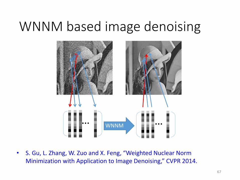
WNNM based image denoising

67

… …WNNM

• S. Gu, L. Zhang, W. Zuo and X. Feng, “Weighted Nuclear Norm Minimization with Application to Image Denoising,” CVPR 2014.

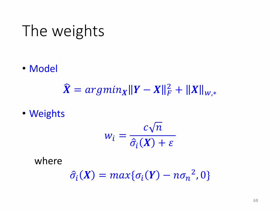
The weights

68

• Model

𝑿 = 𝑎𝑟𝑔𝑚𝑖𝑛𝑿 𝒀 − 𝑿 𝐹2 + 𝑿 𝑤,∗

• Weights

𝑤𝑖 =𝑐 𝑛

ො𝜎𝑖 𝑿 + 𝜀

where

ො𝜎𝑖 𝑿 = 𝑚𝑎𝑥{𝜎𝑖 𝒀 − 𝑛𝜎𝑛2, 0}

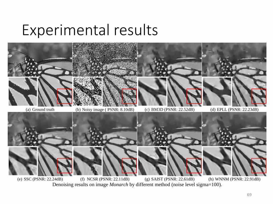
Experimental results

69

(a) Ground truth (b) Noisy image ( PSNR: 8.10dB) (c) BM3D (PSNR: 22.52dB) (d) EPLL (PSNR: 22.23dB)

(e) SSC (PSNR: 22.24dB) (f) NCSR (PSNR: 22.11dB) (g) SAIST (PSNR: 22.61dB) (h) WNNM (PSNR: 22.91dB)

Denoising results on image Monarch by different method (noise level sigma=100).

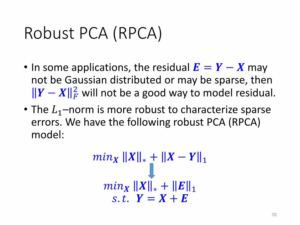
Robust PCA (RPCA)

• In some applications, the residual 𝑬 = 𝒀 − 𝑿 may not be Gaussian distributed or may be sparse, then 𝒀 − 𝑿 𝐹

2 will not be a good way to model residual.

• The 𝐿1–norm is more robust to characterize sparse errors. We have the following robust PCA (RPCA) model:

𝑚𝑖𝑛𝑿 𝑿 ∗ + 𝑿 − 𝒀 1

𝑚𝑖𝑛𝑿 𝑿 ∗ + 𝑬 1𝑠. 𝑡. 𝒀 = 𝑿 + 𝑬

70

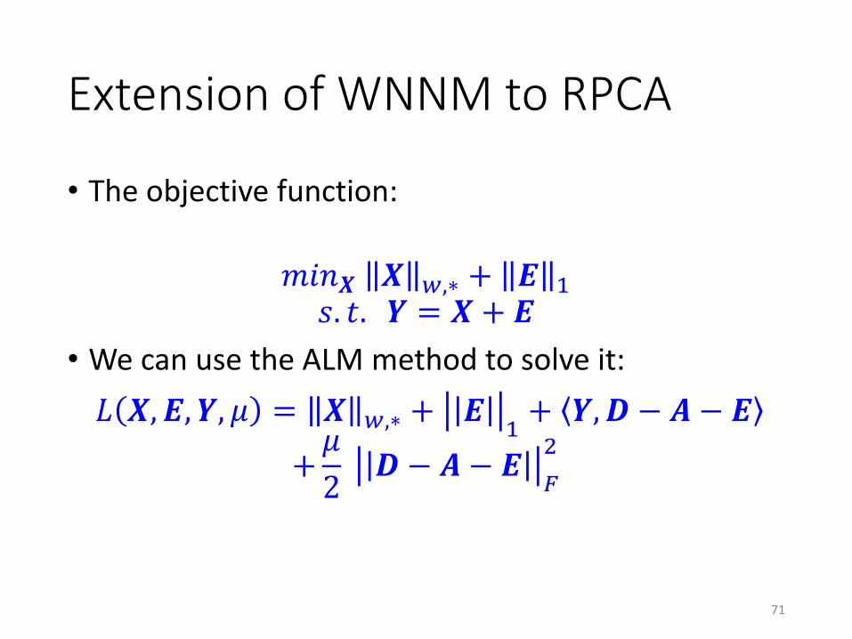
Extension of WNNM to RPCA

• The objective function:

𝑚𝑖𝑛𝑿 𝑿 𝑤,∗ + 𝑬 1𝑠. 𝑡. 𝒀 = 𝑿 + 𝑬

• We can use the ALM method to solve it:

𝐿 𝑿, 𝑬, 𝒀, 𝜇 = 𝑿 𝑤,∗ + 𝑬1+ 𝒀,𝑫 − 𝑨 − 𝑬

+𝜇

2𝑫− 𝑨 − 𝑬

𝐹

2

71

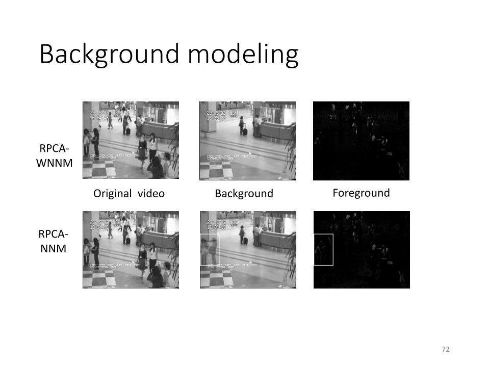
Background modeling

RPCA-NNM

RPCA-WNNM

Original video Background Foreground

72

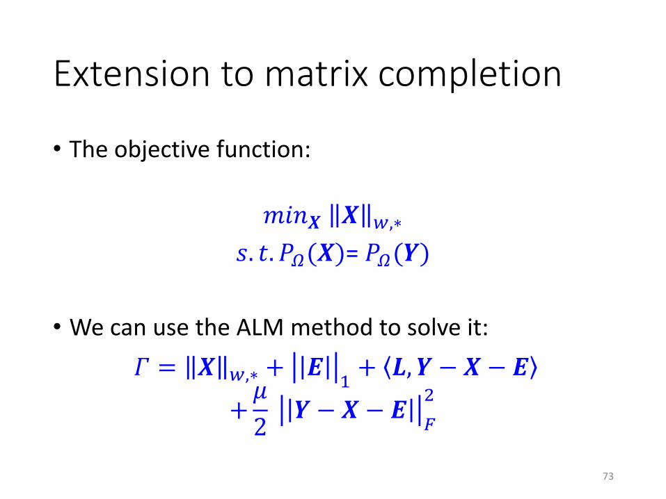
Extension to matrix completion

• The objective function:

𝑚𝑖𝑛𝑿 𝑿 𝑤,∗

𝑠. 𝑡. 𝑃𝛺(𝑿)= 𝑃𝛺(𝒀)

• We can use the ALM method to solve it:

𝛤 = 𝑿 𝑤,∗ + 𝑬1+ 𝑳, 𝒀 − 𝑿 − 𝑬

+𝜇

2𝒀 − 𝑿 − 𝑬

𝐹

2

73

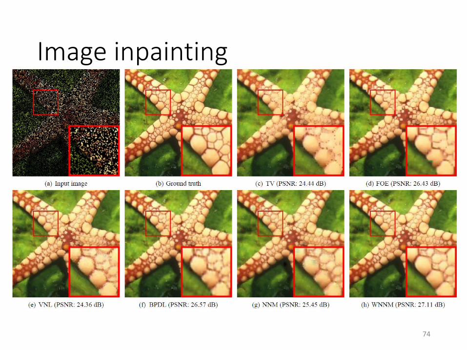
Image inpainting

74

Deep learning for image restoration

75

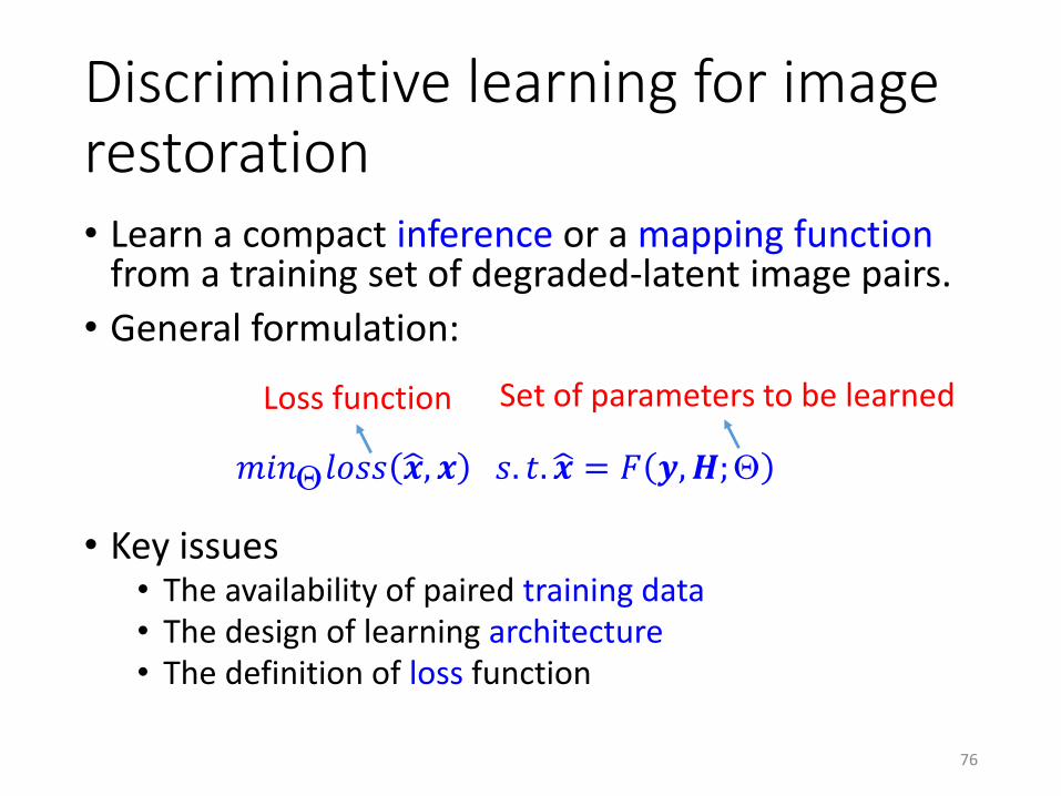
Discriminative learning for image restoration• Learn a compact inference or a mapping function

from a training set of degraded-latent image pairs.

• General formulation:

• Key issues • The availability of paired training data• The design of learning architecture• The definition of loss function

76

𝑚𝑖𝑛𝑙𝑜𝑠𝑠 ෝ𝒙, 𝒙 𝑠. 𝑡. ෝ𝒙 = 𝐹 𝒚,𝑯;

Loss function Set of parameters to be learned

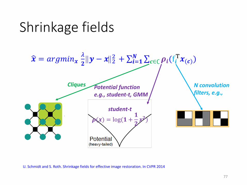
Shrinkage fields

ෝ𝒙 = 𝑎𝑟𝑔𝑚𝑖𝑛𝒙𝜆

𝟐𝒚 − 𝒙2

2 + σ𝒊=𝟏𝑵 σ𝒄∈∁𝝆𝒊(f𝒊

T𝒙(𝒄))

N convolution filters, e.g.,

Cliques Potential functione.g., student-t, GMM

𝝆(𝒙) = log(𝟏 +𝟏

𝟐𝒙𝟐)

student-t

U. Schmidt and S. Roth. Shrinkage fields for effective image restoration. In CVPR 2014

77

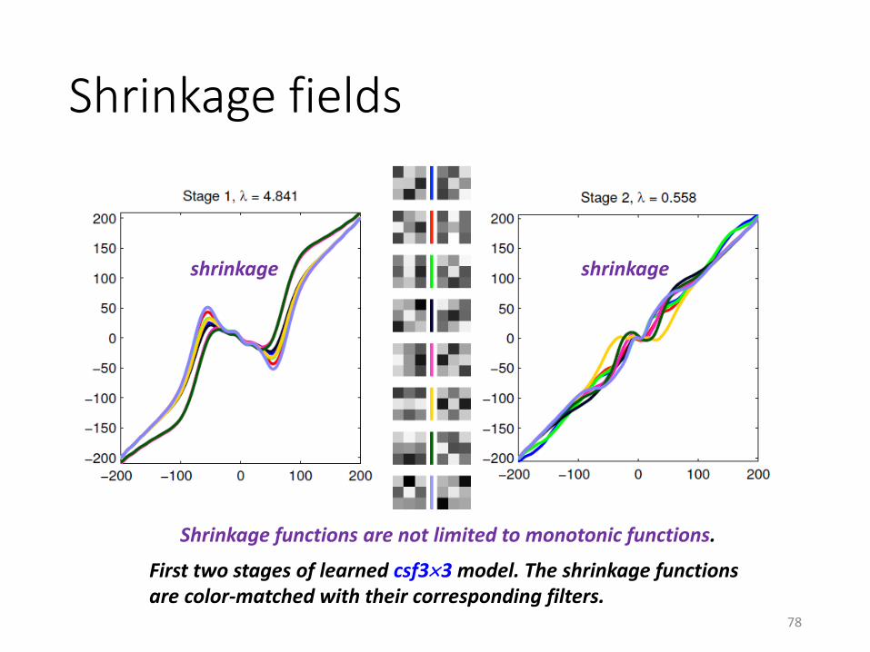
Shrinkage fields

First two stages of learned csf33 model. The shrinkage functionsare color-matched with their corresponding filters.

Shrinkage functions are not limited to monotonic functions.

shrinkage shrinkage

78

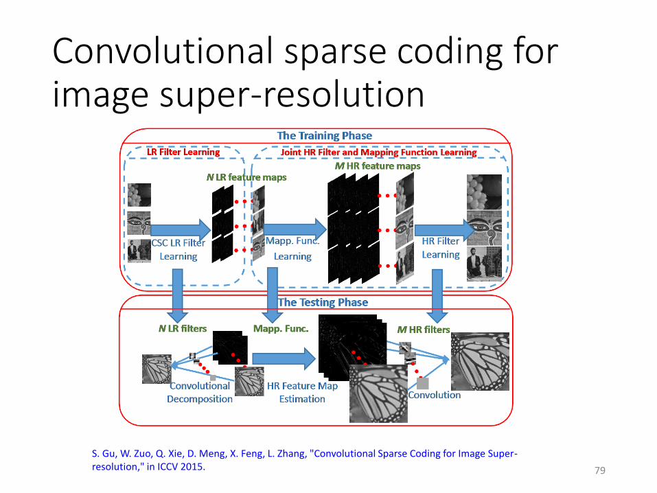
Convolutional sparse coding for image super-resolution

79

S. Gu, W. Zuo, Q. Xie, D. Meng, X. Feng, L. Zhang, "Convolutional Sparse Coding for Image Super-resolution," in ICCV 2015.

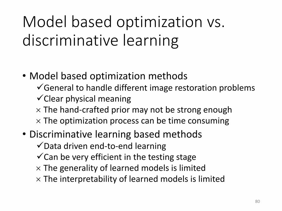
Model based optimization vs. discriminative learning

• Model based optimization methodsGeneral to handle different image restoration problemsClear physical meaning The hand-crafted prior may not be strong enough The optimization process can be time consuming

• Discriminative learning based methodsData driven end-to-end learningCan be very efficient in the testing stage The generality of learned models is limited The interpretability of learned models is limited

80

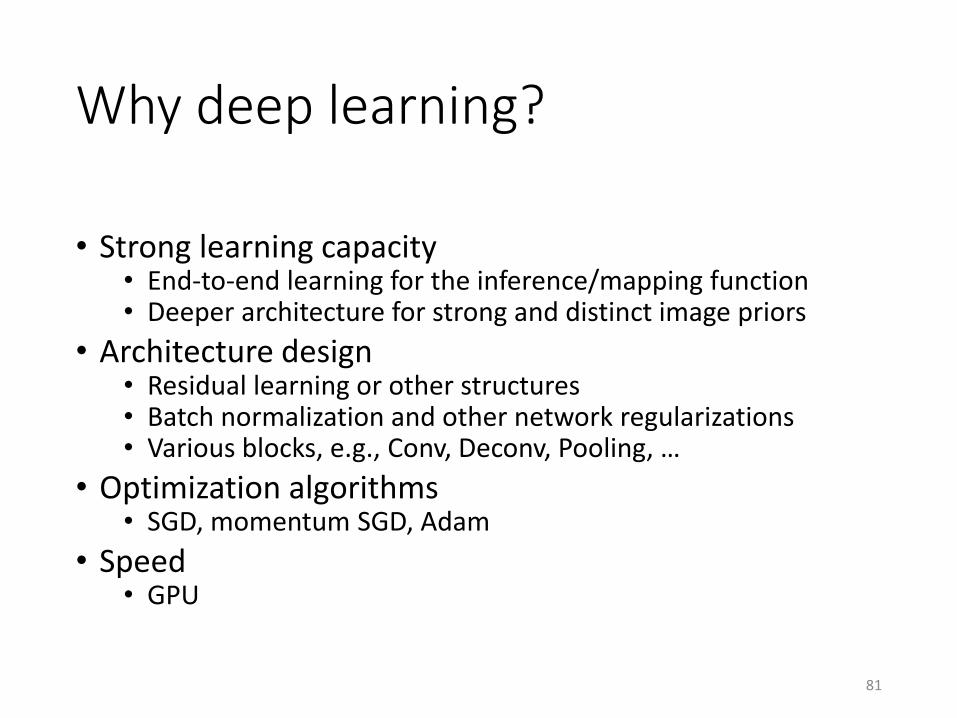
Why deep learning?

• Strong learning capacity• End-to-end learning for the inference/mapping function• Deeper architecture for strong and distinct image priors

• Architecture design• Residual learning or other structures• Batch normalization and other network regularizations• Various blocks, e.g., Conv, Deconv, Pooling, …

• Optimization algorithms• SGD, momentum SGD, Adam

• Speed• GPU

81

82

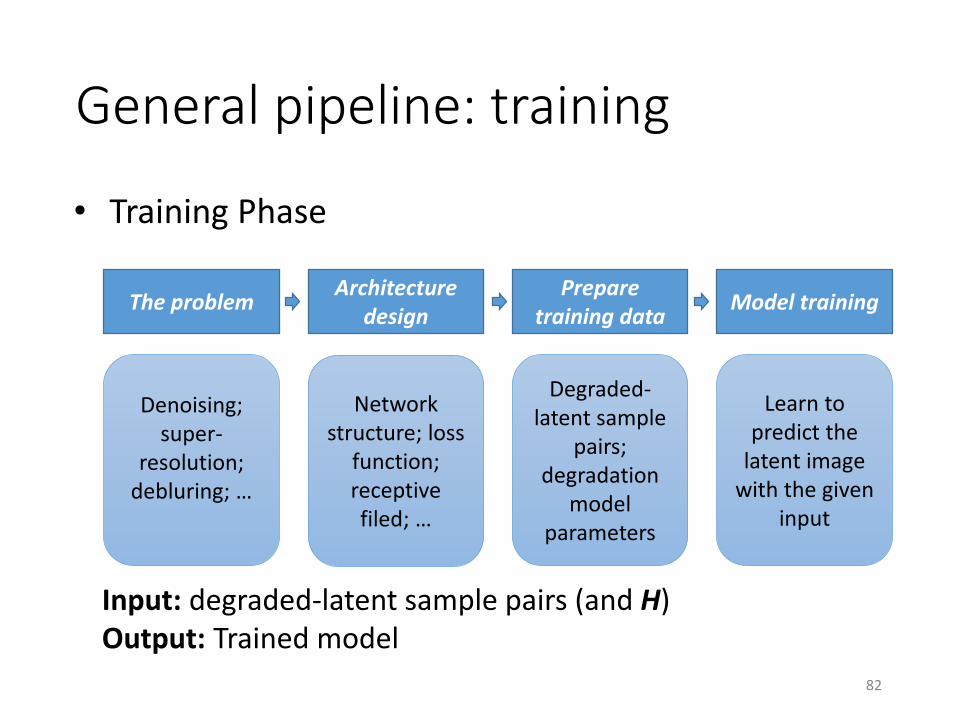
• Training Phase

Architecture design

The problemPrepare

training dataModel training

Denoising; super-

resolution; debluring; …

Network structure; loss

function; receptive filed; …

Degraded-latent sample

pairs;degradation

model parameters

Learn to predict the

latent image with the given

input

Input: degraded-latent sample pairs (and H)Output: Trained model

General pipeline: training

83

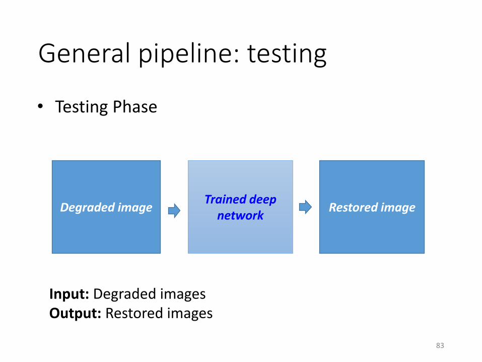
• Testing Phase

Degraded imageTrained deep

networkRestored image

Input: Degraded imagesOutput: Restored images

General pipeline: testing

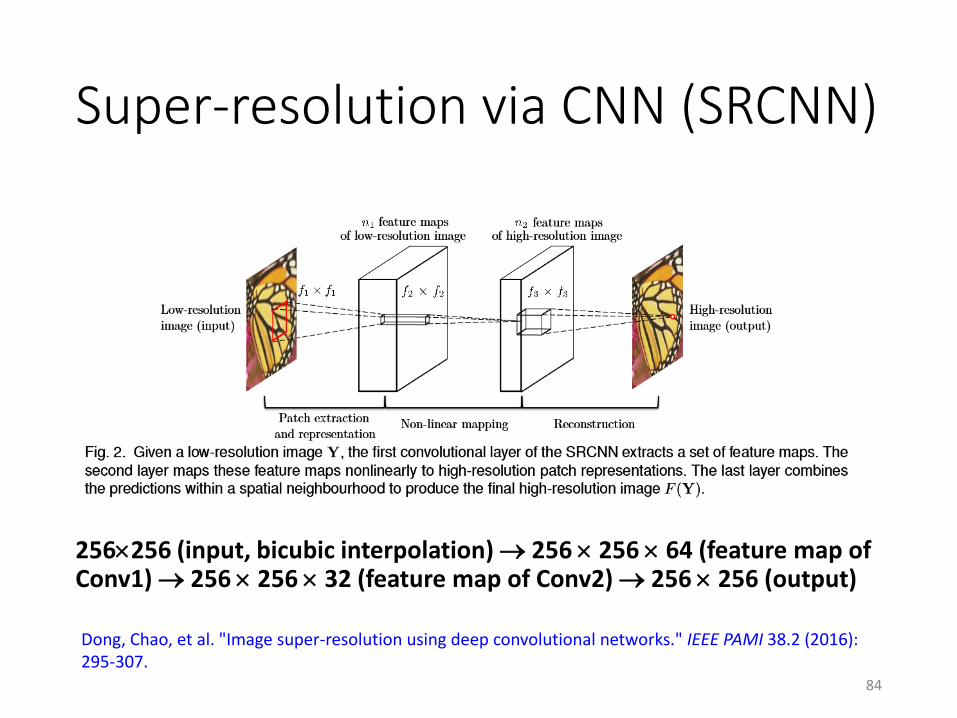
Super-resolution via CNN (SRCNN)

256256 (input, bicubic interpolation) 256 256 64 (feature map of Conv1) 256 256 32 (feature map of Conv2) 256 256 (output)

84

Dong, Chao, et al. "Image super-resolution using deep convolutional networks." IEEE PAMI 38.2 (2016): 295-307.

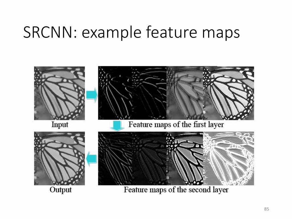
SRCNN: example feature maps

85

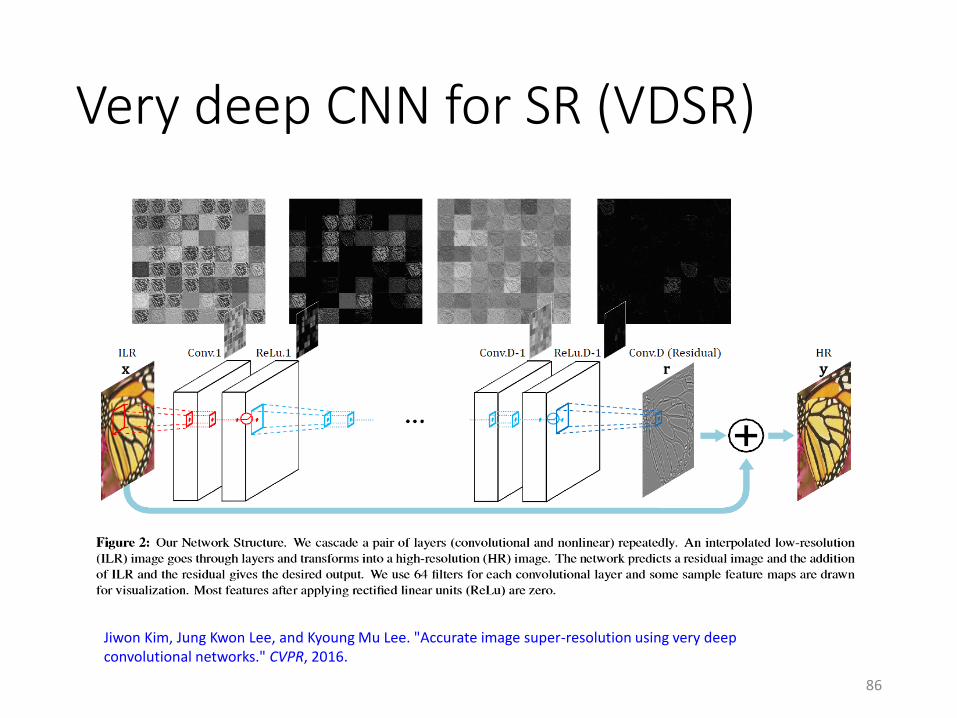
Very deep CNN for SR (VDSR)

86

Jiwon Kim, Jung Kwon Lee, and Kyoung Mu Lee. "Accurate image super-resolution using very deep convolutional networks." CVPR, 2016.

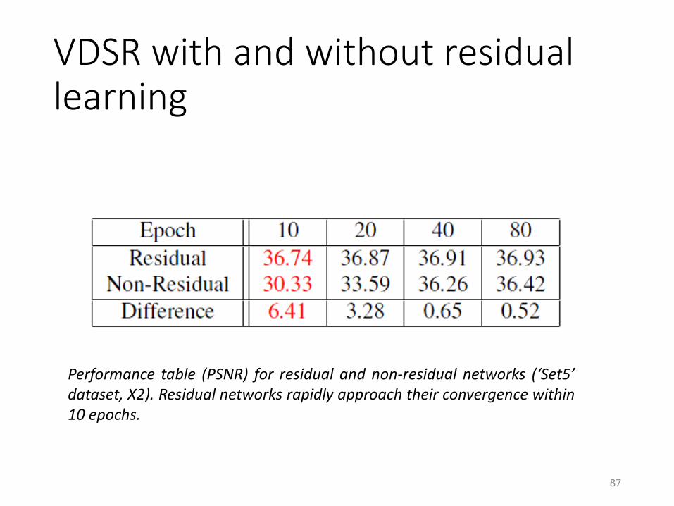
VDSR with and without residual learning

87

Performance table (PSNR) for residual and non-residual networks (‘Set5’dataset, X2). Residual networks rapidly approach their convergence within10 epochs.

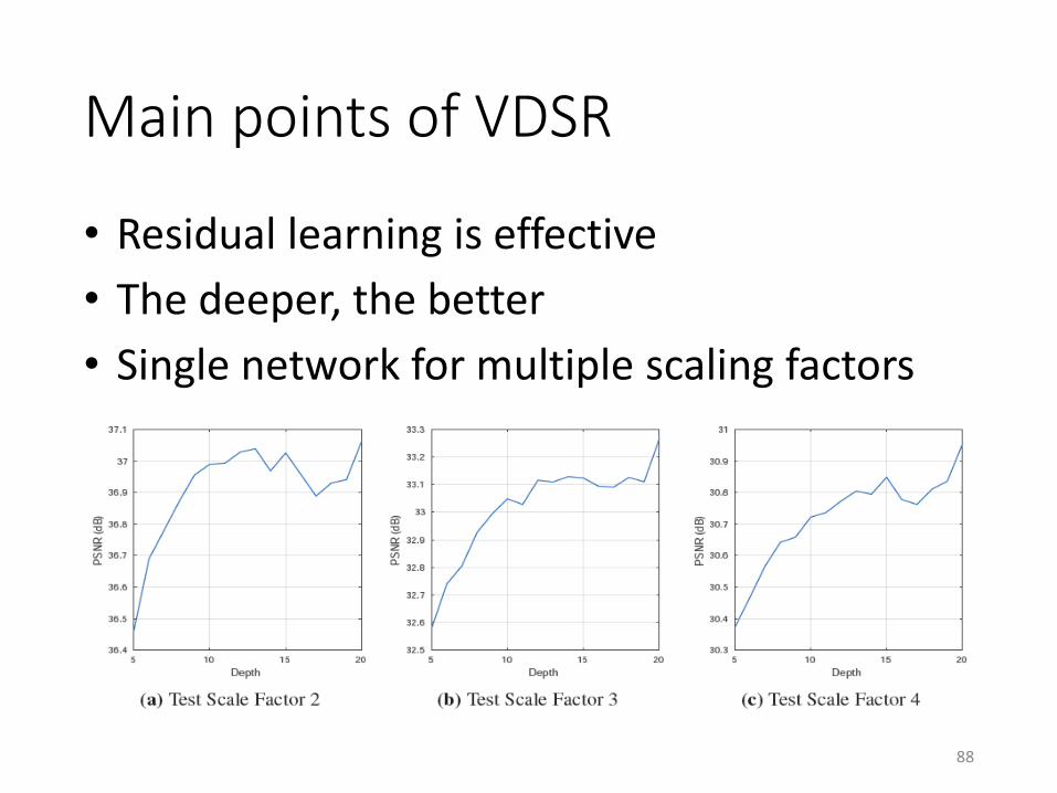
Main points of VDSR

• Residual learning is effective

• The deeper, the better

• Single network for multiple scaling factors

88

89

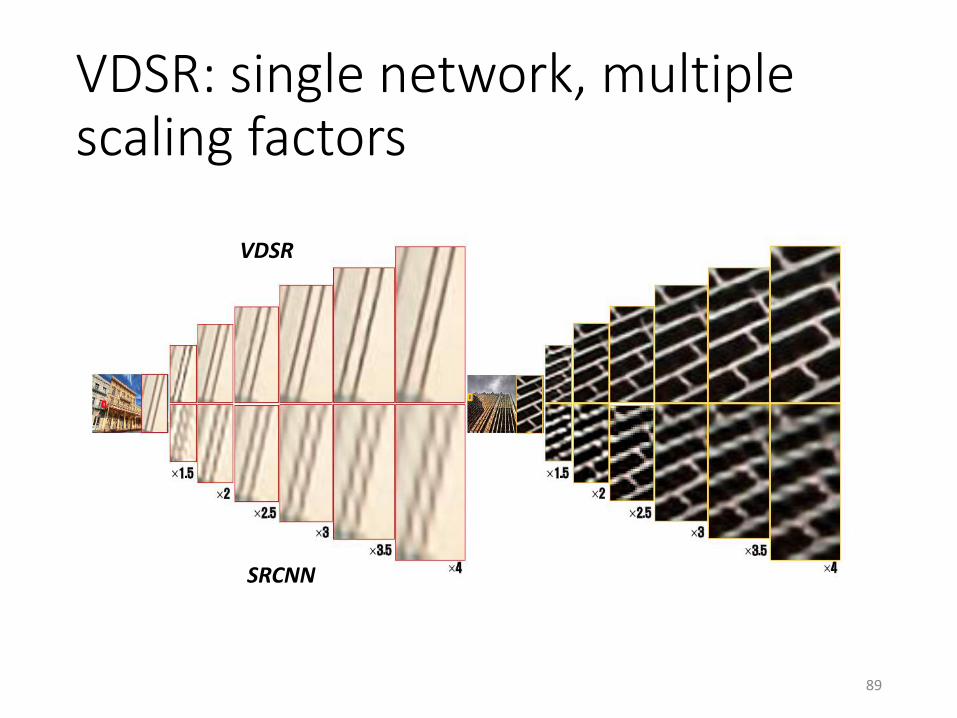
VDSR: single network, multiple scaling factors

VDSR

SRCNN

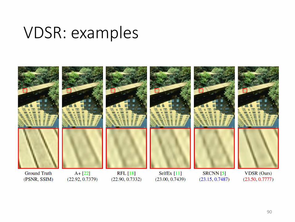
VDSR: examples

90

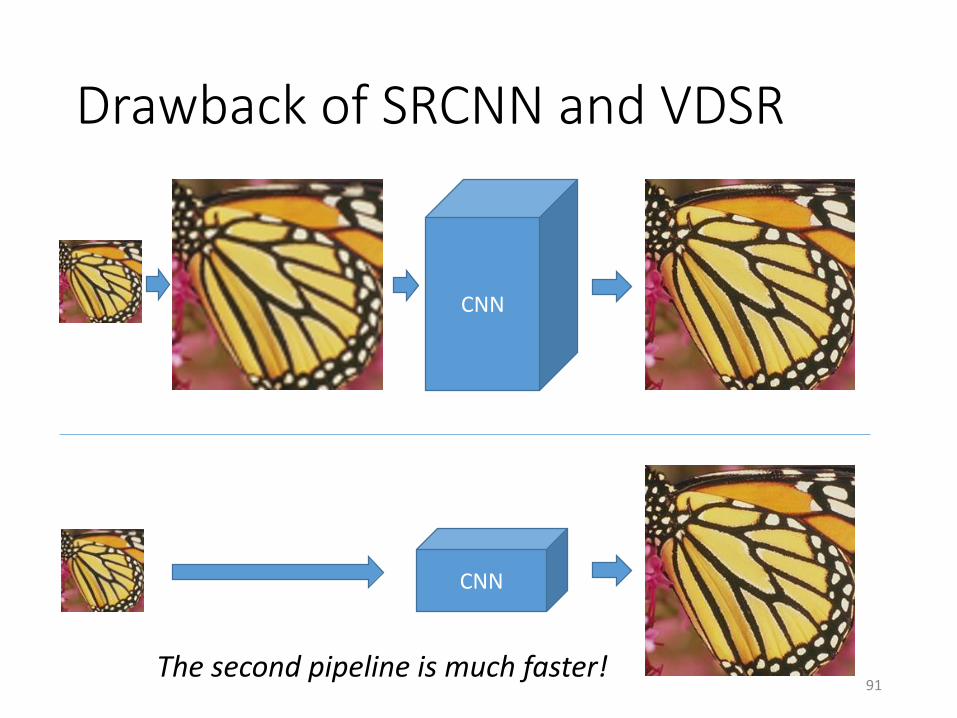
Drawback of SRCNN and VDSR

91

CNN

CNN

The second pipeline is much faster!

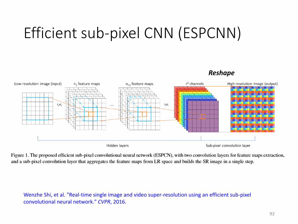
Efficient sub-pixel CNN (ESPCNN)

92

Reshape

Wenzhe Shi, et al. "Real-time single image and video super-resolution using an efficient sub-pixel convolutional neural network." CVPR, 2016.

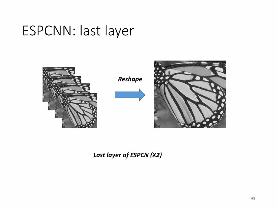
ESPCNN: last layer

93

Last layer of ESPCN (X2)

Reshape

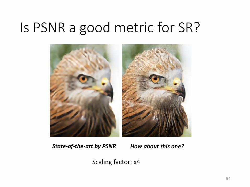
Is PSNR a good metric for SR?

94

State-of-the-art by PSNR How about this one?

Scaling factor: x4

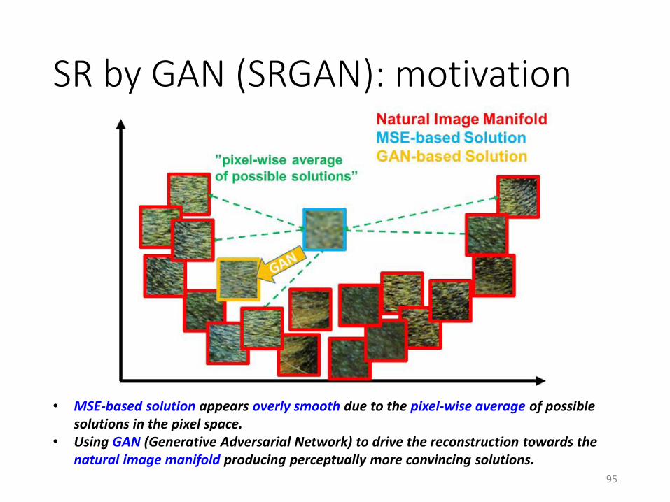
SR by GAN (SRGAN): motivation

95

• MSE-based solution appears overly smooth due to the pixel-wise average of possible solutions in the pixel space.

• Using GAN (Generative Adversarial Network) to drive the reconstruction towards the natural image manifold producing perceptually more convincing solutions.

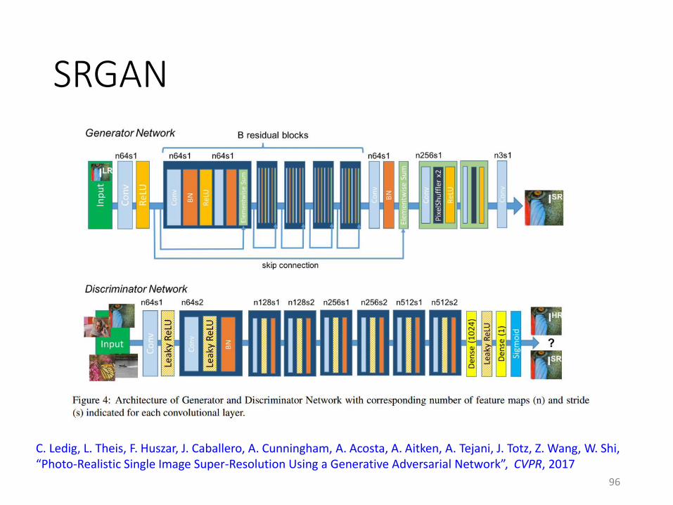
SRGAN

96

C. Ledig, L. Theis, F. Huszar, J. Caballero, A. Cunningham, A. Acosta, A. Aitken, A. Tejani, J. Totz, Z. Wang, W. Shi, “Photo-Realistic Single Image Super-Resolution Using a Generative Adversarial Network”, CVPR, 2017

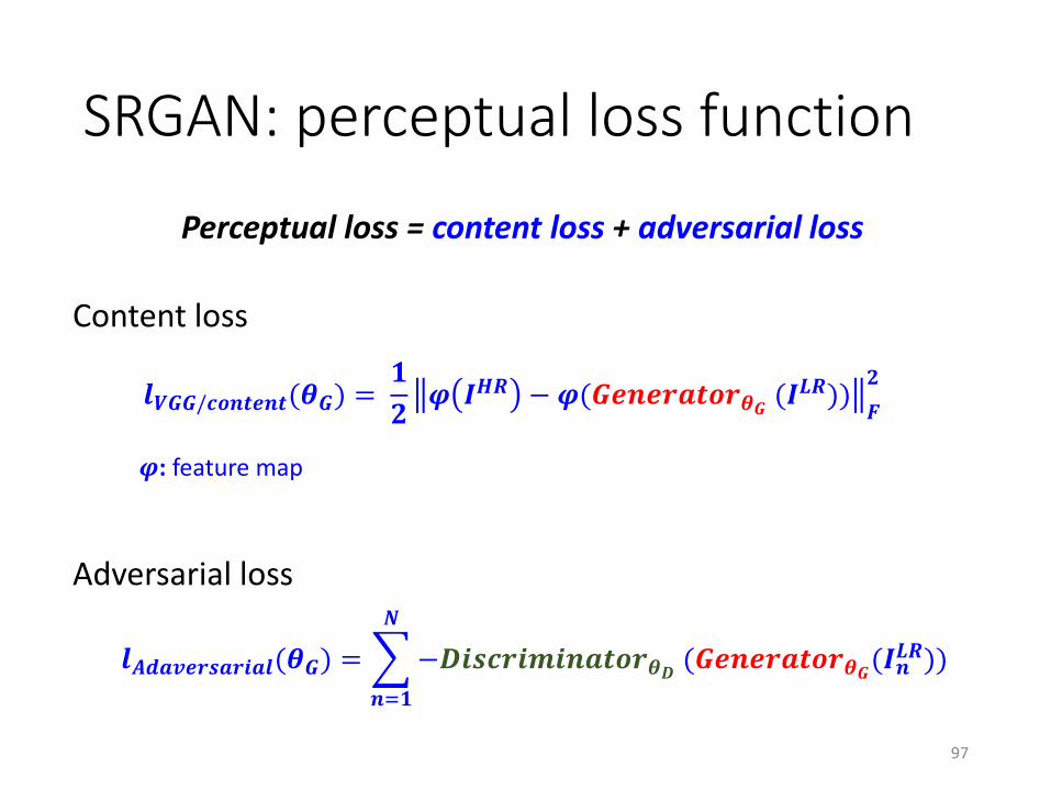
SRGAN: perceptual loss function

97

Content loss

Perceptual loss = content loss + adversarial loss

𝒍𝑽𝑮𝑮/𝒄𝒐𝒏𝒕𝒆𝒏𝒕(𝜽𝑮) =𝟏

𝟐𝝋 𝑰𝑯𝑹 −𝝋(𝑮𝒆𝒏𝒆𝒓𝒂𝒕𝒐𝒓𝜽𝑮 (𝑰

𝑳𝑹))𝑭

𝟐

𝝋: feature map

Adversarial loss

𝒍𝑨𝒅𝒂𝒗𝒆𝒓𝒔𝒂𝒓𝒊𝒂𝒍(𝜽𝑮) =

𝒏=𝟏

𝑵

−𝑫𝒊𝒔𝒄𝒓𝒊𝒎𝒊𝒏𝒂𝒕𝒐𝒓𝜽𝑫 (𝑮𝒆𝒏𝒆𝒓𝒂𝒕𝒐𝒓𝜽𝑮(𝑰𝒏𝑳𝑹))

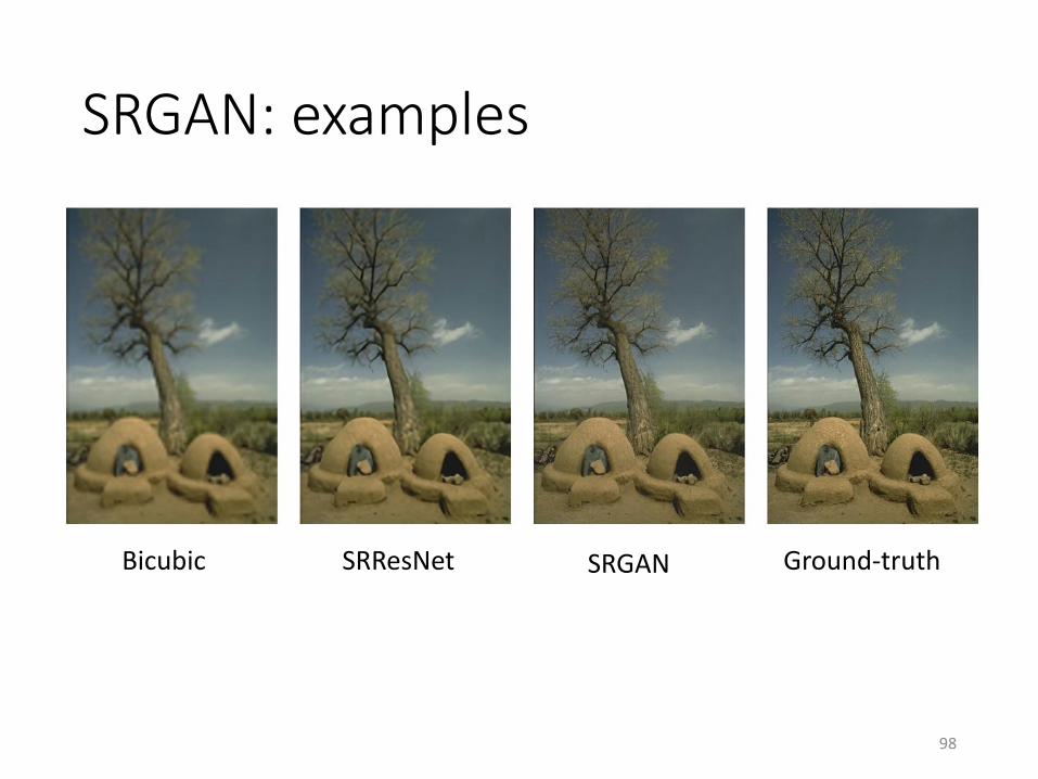
SRGAN: examples

98

Bicubic SRResNet SRGAN Ground-truth

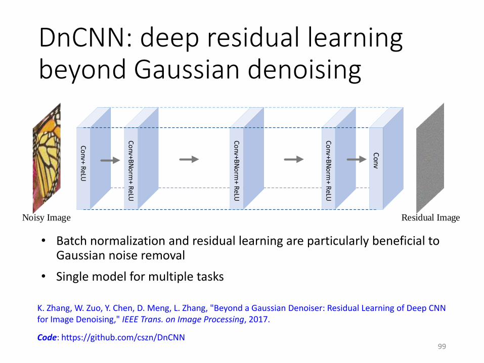
DnCNN: deep residual learning beyond Gaussian denoising

K. Zhang, W. Zuo, Y. Chen, D. Meng, L. Zhang, "Beyond a Gaussian Denoiser: Residual Learning of Deep CNN for Image Denoising," IEEE Trans. on Image Processing, 2017.

Code: https://github.com/cszn/DnCNN99

• Batch normalization and residual learning are particularly beneficial to Gaussian noise removal

• Single model for multiple tasks

Noisy Image Residual Image

Co

nv+ ReLU

Co

nv+BN

orm

+ ReLU

Co

nv+BN

orm

+ ReLU

Co

nv+BN

orm

+ ReLU

Co

nv

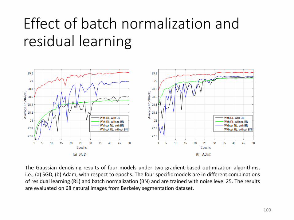
Effect of batch normalization and residual learning

100

The Gaussian denoising results of four models under two gradient-based optimization algorithms,i.e., (a) SGD, (b) Adam, with respect to epochs. The four specific models are in different combinationsof residual learning (RL) and batch normalization (BN) and are trained with noise level 25. The resultsare evaluated on 68 natural images from Berkeley segmentation dataset.

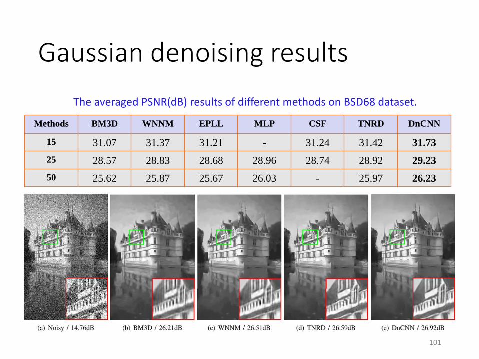
Gaussian denoising results

101

Methods BM3D WNNM EPLL MLP CSF TNRD DnCNN

15 31.07 31.37 31.21 - 31.24 31.42 31.73

25 28.57 28.83 28.68 28.96 28.74 28.92 29.23

50 25.62 25.87 25.67 26.03 - 25.97 26.23

The averaged PSNR(dB) results of different methods on BSD68 dataset.

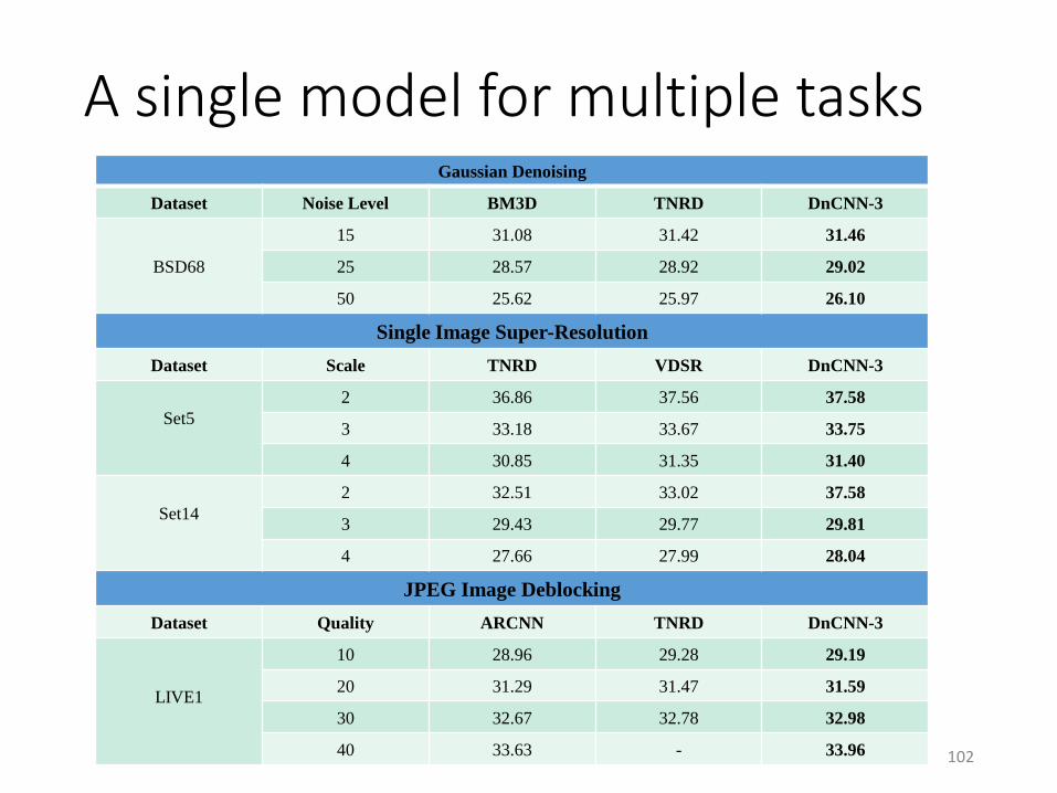
A single model for multiple tasks

102

Gaussian Denoising

Dataset Noise Level BM3D TNRD DnCNN-3

BSD68

15 31.08 31.42 31.46

25 28.57 28.92 29.02

50 25.62 25.97 26.10

Single Image Super-Resolution

Dataset Scale TNRD VDSR DnCNN-3

Set5

2 36.86 37.56 37.58

3 33.18 33.67 33.75

4 30.85 31.35 31.40

Set14

2 32.51 33.02 37.58

3 29.43 29.77 29.81

4 27.66 27.99 28.04

JPEG Image Deblocking

Dataset Quality ARCNN TNRD DnCNN-3

LIVE1

10 28.96 29.28 29.19

20 31.29 31.47 31.59

30 32.67 32.78 32.98

40 33.63 - 33.96

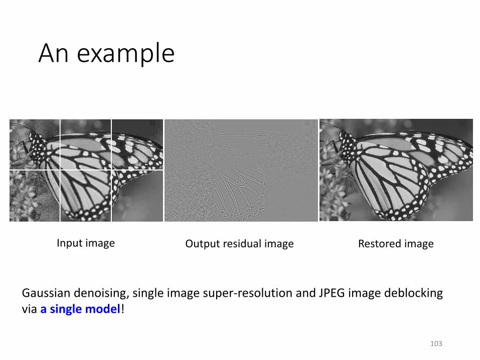
An example

103

Gaussian denoising, single image super-resolution and JPEG image deblockingvia a single model!

Input image Output residual image Restored image

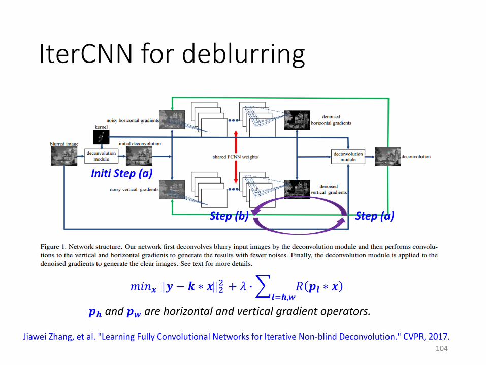
IterCNN for deblurring

104

Initi Step (a)

Step (b) Step (a)

Jiawei Zhang, et al. "Learning Fully Convolutional Networks for Iterative Non-blind Deconvolution." CVPR, 2017.

𝑚𝑖𝑛𝒙 𝒚 − 𝒌 ∗ 𝒙22 + 𝜆 ∙

𝒍=𝒉,𝒘𝑅 𝒑𝒍 ∗ 𝒙

𝒑𝒉 and 𝒑𝒘 are horizontal and vertical gradient operators.

One motivation

• Model based optimization methodsGeneral to handle different image restoration problems

The hand-crafted prior may not be strong enough

• Discriminative learning based methodsData driven end-to-end learning

The generality of learned models is limitted

• Can we integrate the model based optimization and discriminative learning to develop a general image restoration method?

105

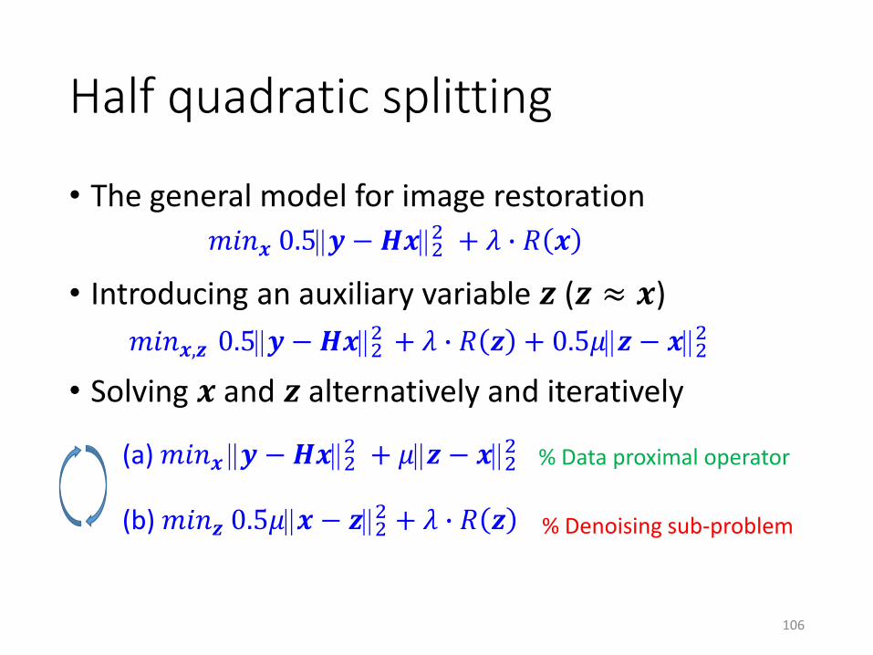
Half quadratic splitting

• The general model for image restoration

• Introducing an auxiliary variable 𝒛 (𝒛 ≈ 𝒙)

• Solving 𝒙 and 𝒛 alternatively and iteratively

106

𝑚𝑖𝑛𝒙 0.5𝒚 − 𝑯𝒙22 + 𝜆 ∙ 𝑅 𝒙

𝑚𝑖𝑛𝒙,𝒛 0.5𝒚 − 𝑯𝒙22 + 𝜆 ∙ 𝑅 𝒛 + 0.5𝜇𝒛 − 𝒙2

2

(a) 𝑚𝑖𝑛𝒙 𝒚 −𝑯𝒙22 + 𝜇𝒛 − 𝒙2

2

(b) 𝑚𝑖𝑛𝒛 0.5𝜇𝒙 − 𝒛22 + 𝜆 ∙ 𝑅 𝒛

% Data proximal operator

% Denoising sub-problem

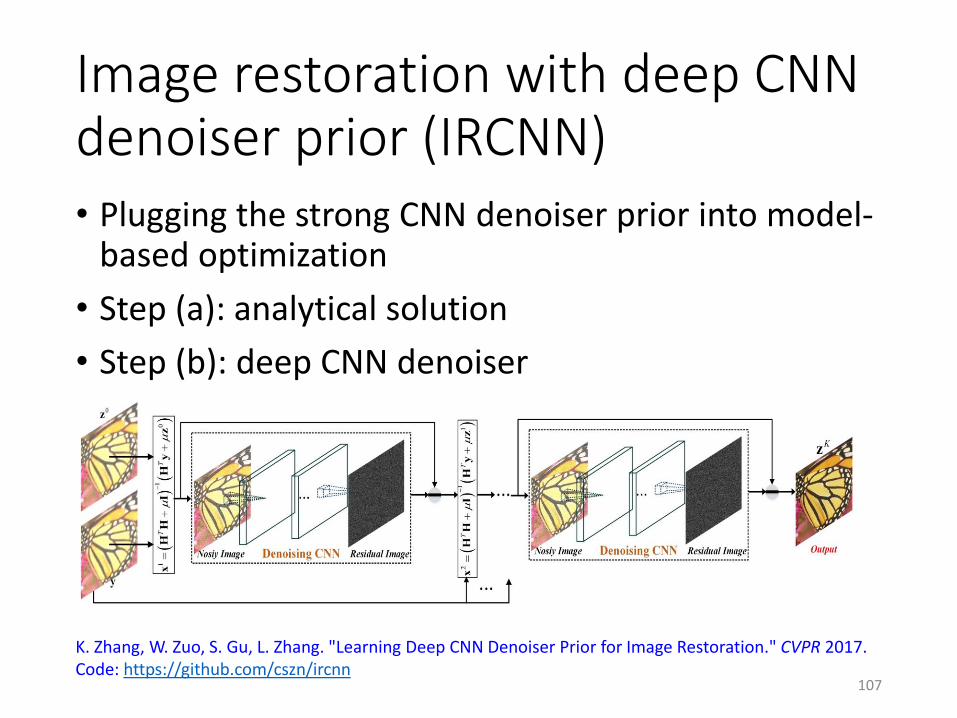
Image restoration with deep CNN denoiser prior (IRCNN)• Plugging the strong CNN denoiser prior into model-

based optimization

• Step (a): analytical solution

• Step (b): deep CNN denoiser

107

K. Zhang, W. Zuo, S. Gu, L. Zhang. "Learning Deep CNN Denoiser Prior for Image Restoration." CVPR 2017.Code: https://github.com/cszn/ircnn

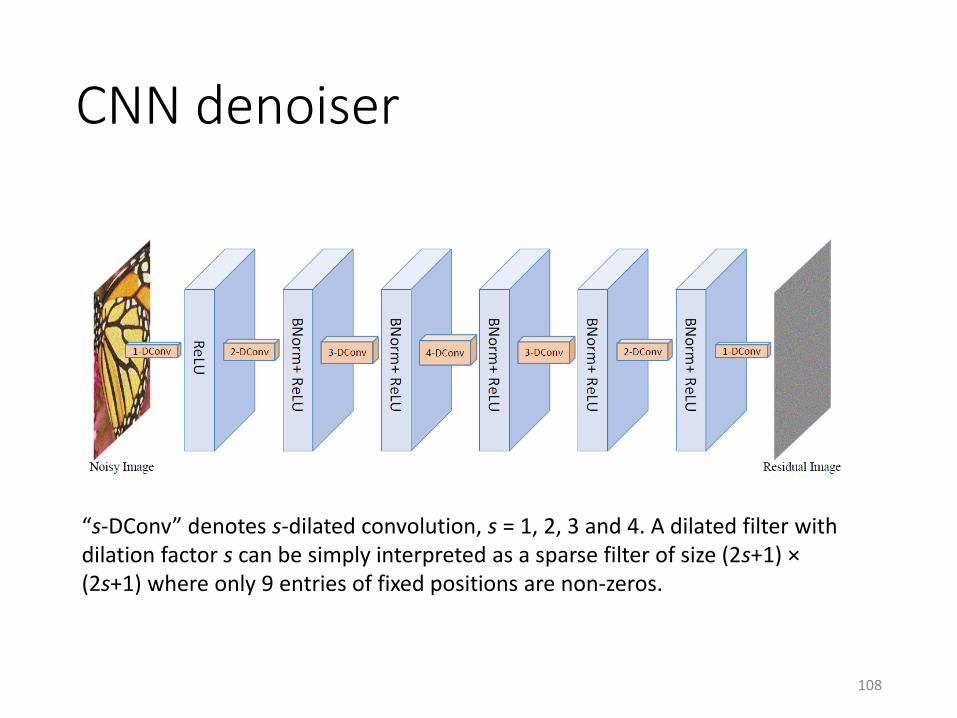
CNN denoiser

108

“s-DConv” denotes s-dilated convolution, s = 1, 2, 3 and 4. A dilated filter with dilation factor s can be simply interpreted as a sparse filter of size (2s+1) ×(2s+1) where only 9 entries of fixed positions are non-zeros.

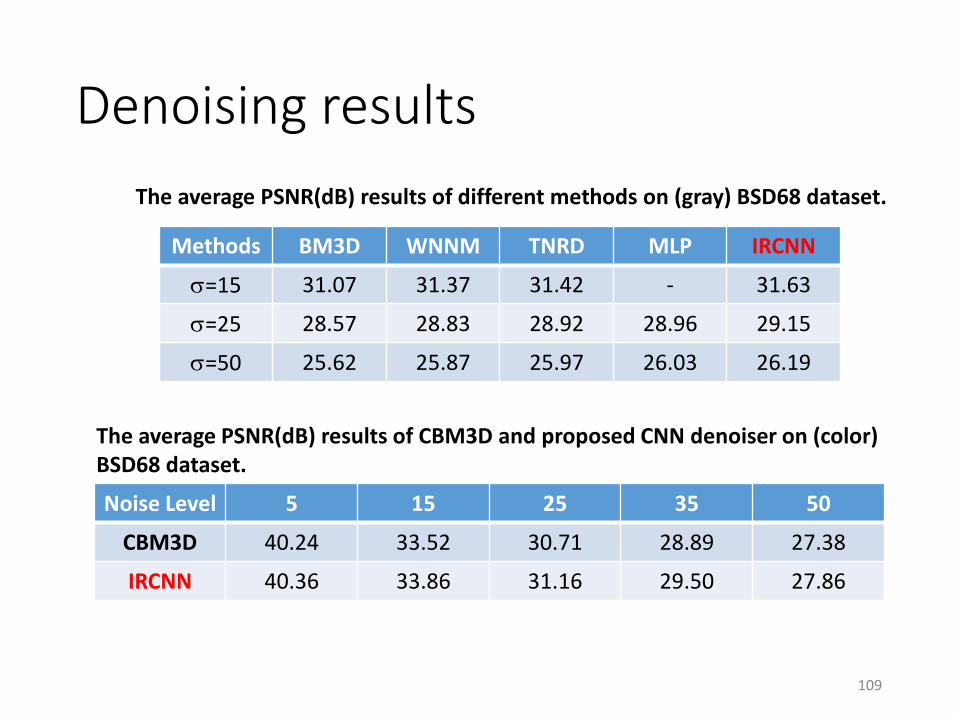
Denoising results

109

Methods BM3D WNNM TNRD MLP IRCNN

=15 31.07 31.37 31.42 - 31.63

=25 28.57 28.83 28.92 28.96 29.15

=50 25.62 25.87 25.97 26.03 26.19

Noise Level 5 15 25 35 50

CBM3D 40.24 33.52 30.71 28.89 27.38

IRCNN 40.36 33.86 31.16 29.50 27.86

The average PSNR(dB) results of different methods on (gray) BSD68 dataset.

The average PSNR(dB) results of CBM3D and proposed CNN denoiser on (color) BSD68 dataset.

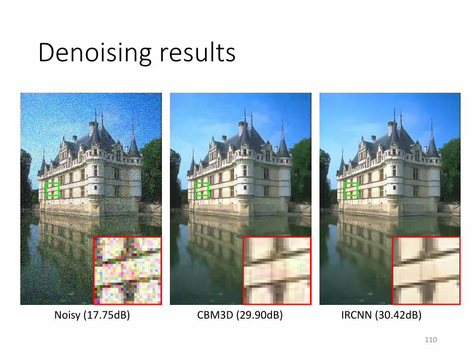
Denoising results

110

CBM3D (29.90dB) IRCNN (30.42dB)Noisy (17.75dB)

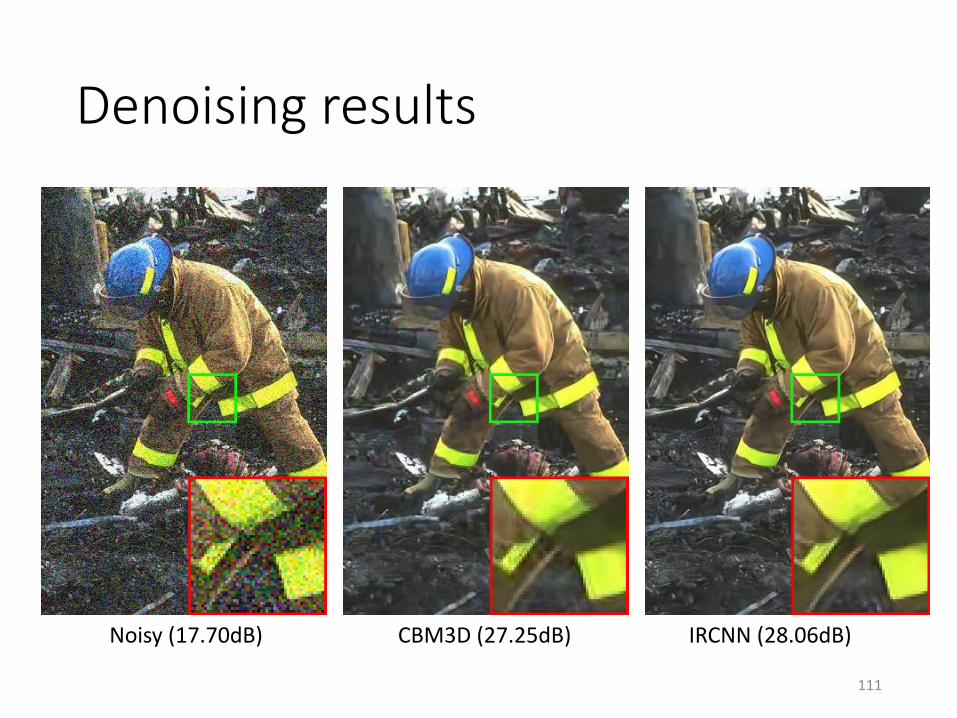
Denoising results

111

CBM3D (27.25dB) IRCNN (28.06dB)Noisy (17.70dB)

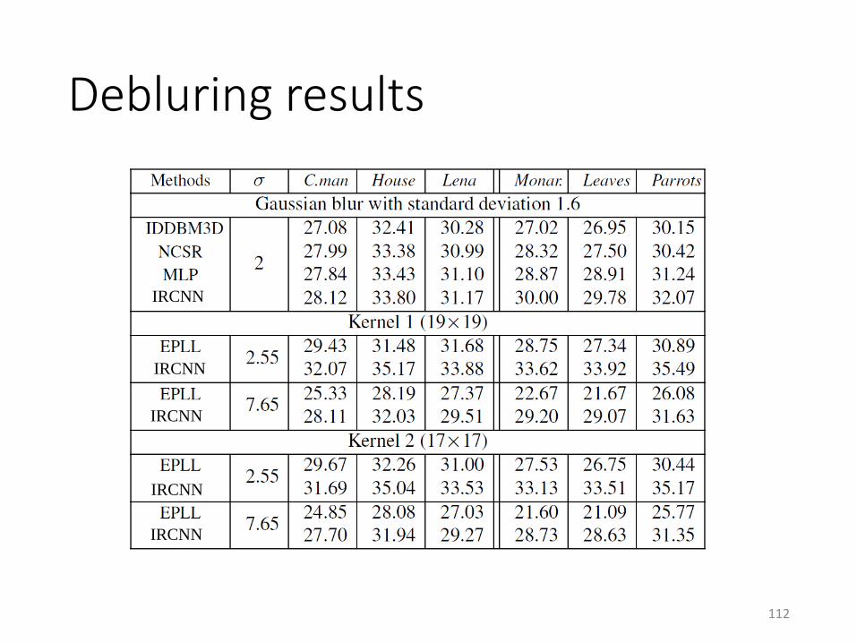
Debluring results

112

IRCNN

IRCNN

IRCNN

IRCNN

IRCNN

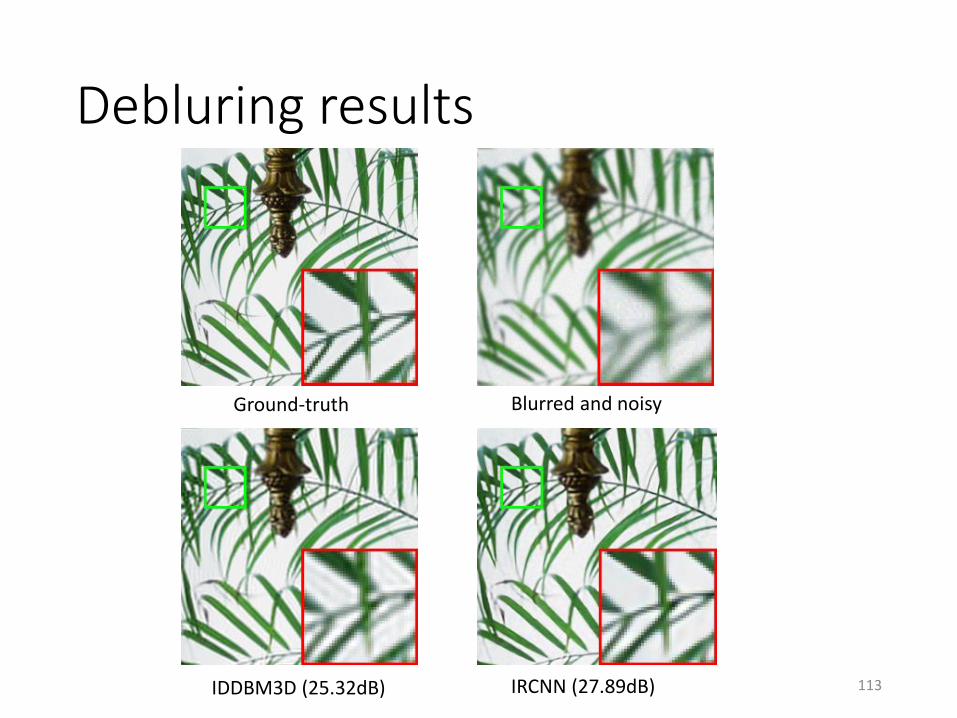
Debluring results

113

Ground-truth Blurred and noisy

IDDBM3D (25.32dB) IRCNN (27.89dB)

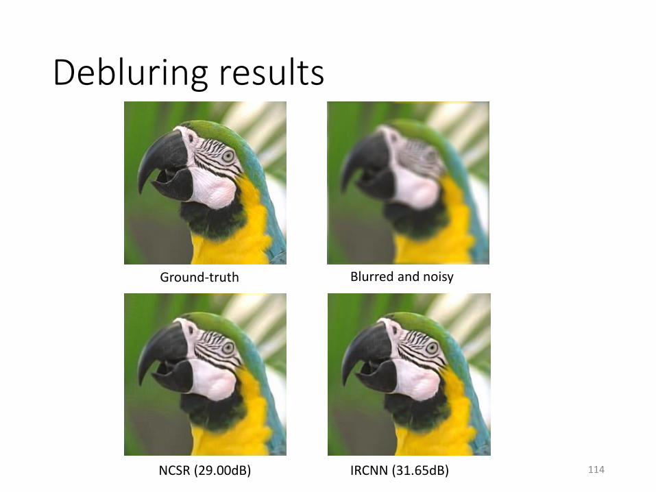
Debluring results

114

Ground-truth Blurred and noisy

NCSR (29.00dB) IRCNN (31.65dB)

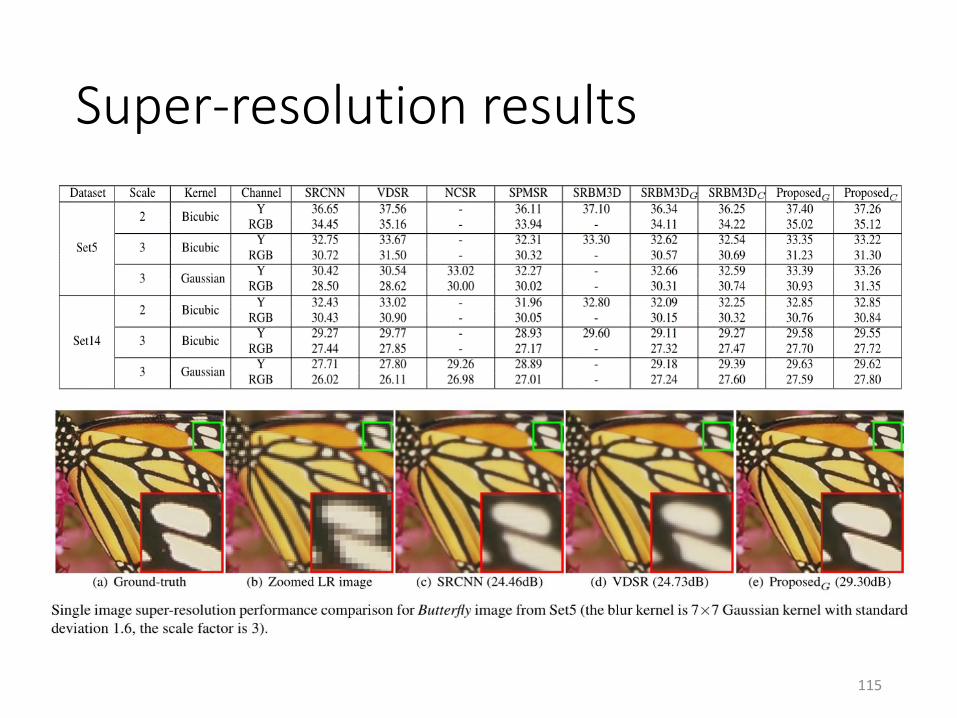
Super-resolution results

115

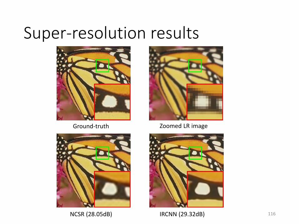
Super-resolution results

116

Ground-truth Zoomed LR image

NCSR (28.05dB) IRCNN (29.32dB)

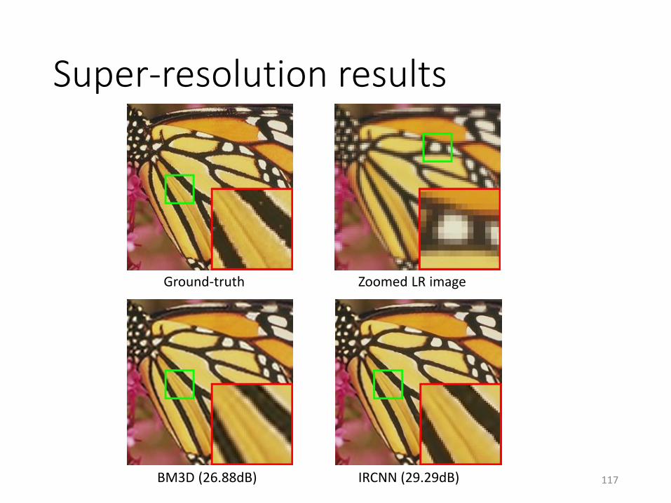
Super-resolution results

117

Ground-truth Zoomed LR image

BM3D (26.88dB) IRCNN (29.29dB)

Open problems

118

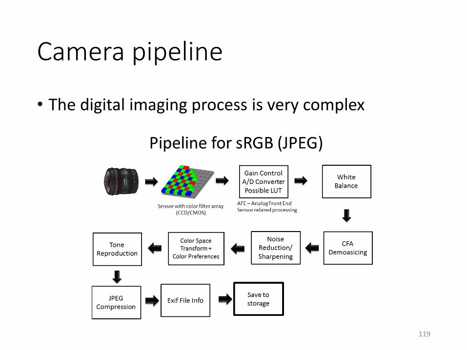
Camera pipeline

119

• The digital imaging process is very complex

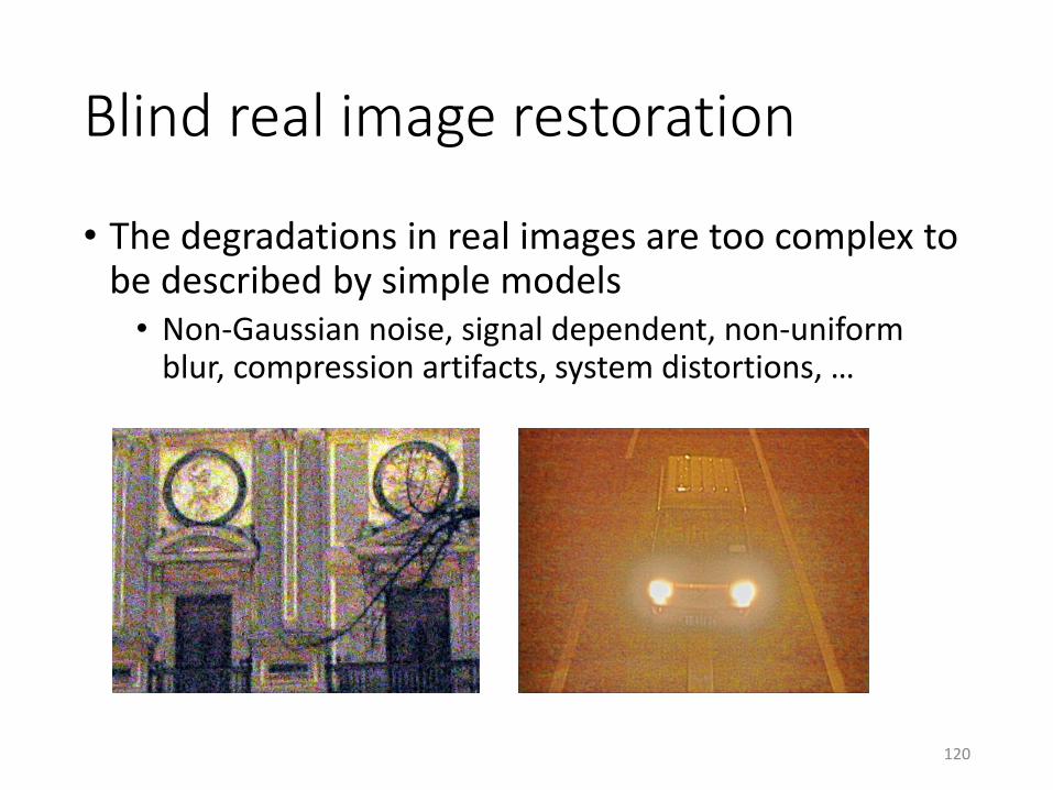
Blind real image restoration

120

• The degradations in real images are too complex to be described by simple models• Non-Gaussian noise, signal dependent, non-uniform

blur, compression artifacts, system distortions, …

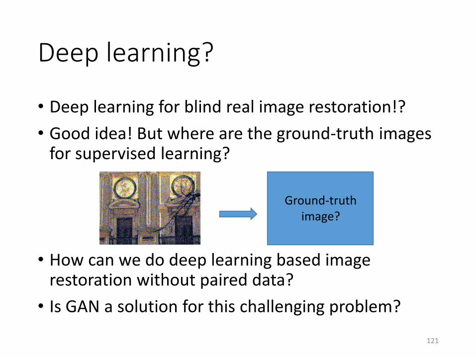
Deep learning?

• Deep learning for blind real image restoration!?

• Good idea! But where are the ground-truth images for supervised learning?

• How can we do deep learning based image restoration without paired data?

• Is GAN a solution for this challenging problem?

121

Ground-truth image?

Summary

122

Summary

• Image sparsity and low-rankness priors have been dominantly used in past decades.

• Recently the CNN based models have been rapidly developed to learn deep image priors.

• There remain many challenging issues for deep learning based image restoration. Key issue: the lack of training image pairs in real-world

blind image restoration applications.

• It is still an open problem to train deep image restoration models without using image pairs.

123

124