Embed Size (px)
Citation preview

11
Image Restoration for Long-Wavelength Imaging Systems
Min-Cheng Pan Department of Electronic Engineering, Tungnan University
New Taipei City Taiwan
1. Introduction
1.1 Overview
Basically, the quality of an image can be evaluated on its spatial and spatial-frequency resolutions, image interpolation and superresolution are perhaps the way to respectively produce high spatial and spatial-frequency resolutions of images especially for a single down-sampled image. For convenience, the term “hyper-resolution” used here represents the approach to enhancing both the spatial and the spatial-frequency resolutions of an image.
As known, the process of decimation or down-sampling is an effective way often used to reduce image sizes, thus, reducing the amount of information transmitted through the communication channels and the local storage requirements, while trying to preserve as much as possible the image quality. Conversely, the reverse procedure of this, referred to as interpolation or up-sampling, is useful in restoring the original high resolution image from its decimated version or for resizing or zooming a digital image. Decimation and interpolation are used for several purposes in many practical applications, such as progressive image transmission systems, multimedia applications, and so forth. A number of conventional interpolation techniques [Hou & Andrews, 1978; Jain, 1989; Keys, 1981] have been proposed to increase the spatial resolution of an image. Undoubtedly, these techniques degrade the quality of the magnified image.
Furthermore, images may be corrupted by degradation such as blurring distortion, noise, and blocking artifacts. These sources of degradation may arise during image capture or processing and have a direct bearing on visual quality. Various methods of restoration have been described in the literature; this diversity reveals the importance of the problem and its great difficulty. The purpose of image deconvolution or restoration is to recover degraded images by removing noise, highlighting image contrast, and preserving edge features of image.
Image superresolution was developed in 1950s to improve image quality and pilot research of this field is derived from the early work (Toraldo di Francia, 1952, 1955) where the term “superresolution” was used in the paper. Following that, clear definition, description and some of the obvious contribution to this field can be found in the work (Gerchberg, 1974; Hunt & Sementilli, 1992) in which their work, superresolution, was meant to seek to recover
www.intechopen.com

Image Restoration – Recent Advances and Applications
230
object information from above the spatial-frequency limit of diffraction. Originally, superresolution referred to a technique of one-frame-to-one-frame and its interest was in the spatial-frequency domain, neither for multi-frames-to-one-frame nor for interpolation. Since then, signal/image restoration/superresolution has been concerned for the spatial-frequency domain from one low-resolution frame to one high-resolution frame; basically, the distinct nature of those algorithms is iterative and nonlinear. A process of interpolation along with restoration/superresolution was used with one frame to enhance the spatial and spatial-frequency resolution of the frame (Pan, 2006). Else, the processing of multi-frame-to-one-frame has been quite concerned (Gillette et al., 1995; Ng et al., 2003; Segal et al., 2003), where a single high-resolution frame was reconstructed from multiple low-resolution frames.
1.2 Long-wavelength imaging system
Image restoration is able to be applied to the long-wavelength imaging systems, millimeter-wave (mm-wave) and near-infrared diffuse optical tomography (NIR DOT) imaging systems, shown as Fig. 1.1.. The advantage of long-wavelength imaging systems is to provide special information with no radioactive characteristics but the physical property of long wavelength with diffraction or scattering results in lower spatial-frequency resolution images, however, which can be improved using image restoration to enhance its applicability.
mm-wave imaging system
*imaging system*fog or drizzle weather
Near infrared diffusive Optical tomography
*imaging system *breast diagnosis
(2D image) post-processing
inter-processing(1D signals2D image)
Long wavelength
Medical Science :Tissue opticsClinical Medicine
Hardware
System:Optoelectronics
Scanning
device
1D signals
Software
System:
Reconstruction
Inter-processing
2D imageHardware System:
OptoelectronicsScanning device
2D image
2D
image resto-ration
Non-radioactive
diffraction
diffusion
low resolution
Fig. 1.1. Long Wavelength Imaging Systems v.s. Image Restoration
Images acquired from millimeter-wave imaging system for the fog or rain weather can be applied to navigation; its image resolution of 2D image can be improved with the technology of image restoration. NIR DOT imaging system provides computed tomography (CT) images of the human body or biological tissue/organ, used in medical diagnosis;
www.intechopen.com

Image Restoration for Long-Wavelength Imaging Systems
231
image processing techniques can improve the image quality of tomographic images between iterations of image reconstruction.
The technique using image restoration gradually becomes popular for an mm-wave or an NIR DOT imaging system; the difference of both imaging systems is that the former is post-processing and the latter is inter-processing.
1.3 Varied algorithms of Image restoration
There are two categories of restoration methods for improving image quality: (i) noniterative restoration such as the inverse filter, the Wiener filter (Wiener, 1942) and (ii) nonlinear iterative restoration/superresolution techniques such as Lorentzian restoration method (Lettington & Hong, 1995), maximum a posteriori (MAP) (Hunt & Sementilli, 1992), Richardson-Lucy (RL) deconvolution method (Richardson, 1972; Lucy, 1974), maximum entropy (Frieden, 1972), projection onto convex sets (Sezan & Tekalp, 1988), Gerchberg error energy reduction process (Gerchberg, 1974), and edge-preserving regularization (Teboul et al., 1998). In these methods, it is essential to use the adequate blurring function (a low-pass filter) to restore a degraded image.
1.4 Remark
In this section, we have described a number of terms such as spatial resolution, spatial-frequency resolution, interpolation, restoration, superresolution, hyper-resolution, inter-processing, and post-processing. In addition, advantages and drawbacks of long wavelength imaging systems were addressed and general description of restoration algorithms was made. It is worth emphasizing that long wavelength imaging systems have the same problem to be dealt with so image restoration can be used to improve such an imaging system.
Following this introduction, this chapter is organized as follows. Section 2 describes mathematical model of image formation; image restoration algorithms and further consideration on image restoration are explained in Sec. 3 and Sec. 4, respectively. Subsequently, Sec. 5 demonstrates related applications of image restoration. Finally, conclusion is drawn in Sec. 6.
2. Mathematical model of Image formation
In this section, imaging systems, image formation model, and forward problem and inverse problem are described in the following.
2.1 Imaging systems
2.1.1 Common imaging system
Usually, the imaging process of a common imaging system is formed as follows. Suppose we have a scene of interest that is going to pass through a common imaging system where it has been corrupted by a linear blurring function and some additive noise. The blurring function h accounts for the imperfectness of the imaging system including optical lens or the human factors in shooting the images. Some typical examples are a diffraction-limited or defocused lens and camera motion or shaking during the exposure. The noise arises from
www.intechopen.com

Image Restoration – Recent Advances and Applications
232
the inherent characteristics of the recording media, e.g., electronic noise and quantization noise when the images are digitized (or discretized).
In practice, the available blurred image not only follows exactly the above description but also is constrained with the film size, in most cases the images have to be truncated at the boundaries. Instead, what is available now becomes a windowed blurred image where a rectangular window is usually accounting for the film aperture shape and size. One inherent problem with this is that many ringing artifacts are introduced into the restored image when the linear or nonlinear filter is applied directly to the truncated blurred image.
2.1.2 Medical imaging system
Here, we use NIR DOT imaging system as an example. Basically, an NIR DOT imaging system is composed of a measuring instrument associated with image reconstruction scheme for the purpose of reconstructing the NIR optical-property tomographic images of phantoms/tissue of interest. The reconstructed images reveal the NIR optical properties of tissue computed by using measured radiances emitted from the circumference of the object. A schematic diagram of the NIR DOT measuring system in the frequency domain is shown in Fig. 2.1.
Fig. 2.1. Schematic diagram of NIR DOT measuring system in the frequency domain.
2.2 Image formation model
The image formation is modelled as
g f h n (2.1)
where f is the original scene, h is the point-spread function (p.s.f.) of the imaging system,
is the convolution operator, n is the noise, and g is the corrupted image. Subsequently, the corrupted image is windowed due to the film size/support area and sampled for digitization.
Aliasing is arising, which causes different signals to become indistinguishable when sampled. It also refers to the distortion or artifact that results when the signal reconstructed from samples is different from the original continuous signal.
www.intechopen.com

Image Restoration for Long-Wavelength Imaging Systems
233
2.3 Forward problem & inverse problem
In a common imaging system, the image is formed as the above description in which finding an estimated original signal/image (f) is an inverse problem for a given corrupted signal/image (g) while the reverse process is a forward problem. In tomographic imaging, the reconstruction of optical-property images is done iteratively using a Newton method, requiring inversion of a highly ill-posed and ill-conditioned matrix. The goal of DOT is to estimate the distribution of the optical properties in tissue from non-invasive boundary measurements. For the purpose of determining the optical properties (the absorption coefficient and the diffusion/scattering coefficient) from measurement data, which is an inverse problem in DOT, a forward model is needed to describe the physical relation between the boundary measurements of tissue and the optical properties that characterize the tissue.
2.3.1 Forward problem in DOT
In general, such a forward model of NIR DOT that gives the description of this physical relation is the diffusion equation,
, , ,a
iS
c
r r r r r (2.2)
where , r is the photon density at position r and is the light modulation frequency. ,S r is the isotropic source term and c is the speed of light in tissue. a and denote the optical absorption and diffusion coefficients, respectively. In addition, the finite element method (FEM) and a Robin (type-III) [Brendel & Nielsen, 2009; Holboke et al., 2000] boundary condition are applied on Eq. (2.2) to solve this forward problem, i.e., calculating the photon density for a given set of optical property within the tissue.
2.3.2 Inverse problem in DOT
Owing to the non-linearity with respect to the optical properties, an analytic solution to the inverse problem in DOT is absent. Instead, the numerical way of obtaining the inverse solution is to iteratively minimize the difference between the measured diffusion photon density data, MΦ , around the tissue and the calculated model data, CΦ , from solving the forward problem with the current estimated optical properties. This data-model misfit difference is typically defined as follows,
22
1
MNC Mi i
i
(2.3)
where MN is the number of measurements.
By means of the first order Taylor series to expandΦ , one can get Eq. (2.4),
,C CM C
aa
Φ ΦΦ Φ μ κμ κ
(2.4)
www.intechopen.com

Image Restoration – Recent Advances and Applications
234
since the goal is to reach MΦ from the current CΦ , and, thus, MΦ and CΦ have been used in the left and right parts of Eq. (2.4), respectively. As well, the vector aμ and κ denote the updates respectively for a and with dimension NN , the number of total nodes in the finite element mesh, and the dimension of the matrices C
a Φ μ or
C Φ κ is M NN N . From Eq. (2.4), the inverse problem in DOT can be formulated as
,C Ca M C
a
μΦ Φ Φ Φκμ κ
(2.5)
or simply denoted as J χ Φ , where C Ca
J Φ μ Φ κ is the Jacobian matrix, the rate of change of model data with respect to optical parameters.
However, solving this linearized inverse problem from Eq. (2.5) usually runs into difficulty with an ill-conditioned problem which typically happens as the number of model parameters increases, so as to solve the inverse problem by means of regularization to remedy such a drawback.
2.4 Remark
In this section, we have explained a common imaging system which includes the operation of convolution, support area, sampling, and noise as well as a medical imaging system of which the optical-property images are formed with the reconstruction algorithm from 1D signals.
3. Image restoration algorithms
This section will discuss non-iterative, iterative and statistical methods; in addition, regularization is also used frequently in image restoration algorithms. More descriptions are explained in the following.
As known, the image degradation is basically modelled as
g f h n (3.1)
where f is the original scene, h is the point-spread function (p.s.f.) of the imaging system, is the convolution operator, n is the noise, and g is the corrupted image.
Generally, the non-linear iterative restoration algorithms (Archer & Titterington, 1995; Hunt, 1994; Meinel, 1986; Singh et al., 1986; Stewart & Durrani, 1986) to enhance image quality by restoring the high frequency spectrum of the corrupted images can be simply modelled as the following form:
1~n n nf f f (3.2)
1( , , , )n nf f g h (3.3)
where the subscript n is the n-th iteration, Eqs. (3.2) and (3.3) represent that a new update (fn) is equal to a previous one (fn-1) plus an updating increment ( nf ). Furthermore, the update ( nf ) is related to the function (Ψ) of the previous update, the corrupted image,
www.intechopen.com

Image Restoration for Long-Wavelength Imaging Systems
235
p.s.f., and a user-defined weight (α). Ψ can have various forms derived from the different algorithms. As known, there are several approaches to enhancing image quality including non-iterative restoration algorithms such as a Gaussian filter and non-linear iterative algorithms such as Poisson maximum a posteriori superresolution algorithm.
3.1 Non-iterative methods
Non-iterative restoration algorithms are described in this sub-section such as the inverse and Wiener filters usually recovering the spatial-frequencies below the diffraction limit. Filters in the Fourier domain are respectively given by the following expressions:
Inverse Filter = 1
H (3.4)
However, Eq. (3.4) is not able to be directly implemented; usually, one uses a so called pseudo-inverse filter with a small constant ┝ as below.
Pseudo-inverse Filter = 1
H (3.5)
Wiener filter is described as Eq. (3.6) in the following.
Wiener Filter = 2
n f
*
[ / ]
H
H (3.6)
where H is the modulation transfer function (MTF) of p.s.f.; the superscript asterisk (*) denotes the complex conjugate; [n/f], the ratio of noise-to-signal. n and f represent the power spectral densities for noise and the true images, respectively. Apparently, applying the Wiener filter to the restoration problem has to know the power spectral densities for the noise and the original image (or more precisely, their ratio). Unfortunately, this a priori knowledge is not available in most cases. Nevertheless, the noise-to-signal ratio (NSR), [n/f], is usually approximated by a small constant ┝. In such a case, the Wiener filter becomes
2
*H
H (3.7)
Wiener filtering achieves a compromise between the improvement obtained by boosting the amplitude of spatial-frequency coefficients up to the diffraction limit and the degradation that occurs because of the noise amplification of the inverse filtering. Noise propagation tends to be reduced by the convolution with p.s.f.; this has a smoothing effect in the result. This fact reveals that Wiener filtering is more immune to noise than inverse filtering.
3.2 Iterative methods
3.2.1 Recursive wiener filter
This technique is briefly described here; further, a more detailed description of the im-plementation of this algorithm can be found in the literature [Kundur & Hatzinakos, 1998].
www.intechopen.com

Image Restoration – Recent Advances and Applications
236
Briefly, such a recursive Wiener-like filtering operation in the Fourier domain can be expressed as Eqs. (3.8) and (3.9).
1
*
2 2
1 1
ˆ.ˆˆ ˆ/
n
n
n n
G FH
F H
(3.8)
1
*1
2 2
1
ˆ.ˆˆ ˆ/
n
nn
n
G HF
H F
(3.9)
The real constant α represents the energy of the additive noise and is determined by prior knowledge of the noise contamination level, if available. The algorithm is run for a specified number of iterations or until the estimates begin to converge. The method is popular for its low computational complexity. The major drawback of the method is its lack of reliability. The uniqueness and convergence properties are, as yet, uncertain.
3.2.2 Lucy-Richardson method
The Richardson–Lucy algorithm, also known as Lucy–Richardson deconvolution, is an iterative procedure for recovering a latent image that has been blurred by a known point spread function.
The Richardson-Lucy (RL) algorithm has been widely used for the data from astronomical imaging. The RL algorithm (Richardson, 1972; Lucy, 1974) generates a restored image through an iterative method, which is derived using a Bayesian statistical approach to guess the original image (f ), to convolute it (fn-1) with the p.s.f. (h) and to compare the result with the real image (g). Usually the guessed image for the first iteration is the blurred image. It uses such an iterative approach:
*1
1n n
n
gf h
f h f (3.10)
3.3 Statistical methods
3.3.1 Poisson MAP algorithm
The Poisson MAP superresolution algorithm begins with Bayes’ law associated with Poisson models for the statistics of image and object to estimate the object by finding the maximum probability on the object (f) given the image (g). Mathematically, the Poisson MAP (Hunt & Sementilli, 1992) is given by
1 11
1n n nn
gf f h f C
f h
exp (3.11)
where represents a convolution; *, a correlation; nf , the restored signal/image; g is the blurred signal/image; h, p.s.f.; 0f , the initial guess signal/image; subscript n, the iteration number. Here,
www.intechopen.com

Image Restoration for Long-Wavelength Imaging Systems
237
1
1n
gh
f h C exp (3.12)
C can be regard as the correction term during the iterative restoration process. In terms of the operation of the Poisson MAP, it is an iterative algorithm where successive estimate of the restored image is obtained by multiplication of the current estimate by a quantity close to one. The quantity close to one is a function of the detected image divided by a convolution of the current estimate with p.s.f.. Indeed, one can replace the exponential in Eq. (3.12) by the first order approximation ex ~ 1+x because of low contrast in a blurred signal/image to achieve Eq. (3.13).
1
~ 1 1n
gh
f h C (3.13)
Thus, Eq. (3.11) can approach to Eq. (3.14).
1 1 11
~ 1n n n n nn
gf f h f f
f h
f (3.14)
Equation (3.14) shows that the Poisson MAP superresolution is consistent with Eq. (3.2). Experience reveals that when implemented for simple point objects, the Poisson MAP algorithm is able to expand the bandwidth much more than done for more complex objects and the Poisson MAP superresolution algorithm requires hundreds of iterations for a final solution.
3.3.2 Improved P-MAP
Following that, the Poisson MAP can be improved by itself by operating upon the edge map with a re-blurring technique; that is, the g and fn-1 of the Poisson MAP are replaced by the corresponding gradients of the g ⊗ h and fn-1 along with the integrated p.s.f. (h ⊗ h). Mathematically, it is shown that
11
( )'( )' ( 1 ( )
( )' ( )n nn
g hf f h h
f h h
)'exp (3.15)
Thus, the final hyper-resolved image f can be obtained by integrating (fn)’. The whole process of this improved Poisson MAP includes re-blurring, differentiation, restoration, integration, and then correction for a DC offset. More details concerning this algorithm can be found in the author’s previous work [Pan, 2003].
3.4 Regularization
Regularization presents a very general methodology for image restoration. The main technique of a regularization procedure is to transform this ill-posed problem into a well-posed one. Roughly speaking, restoration problem with regularization comes down to the minimization problem [Chen et al., 2000; Landi, 2007].
www.intechopen.com

Image Restoration – Recent Advances and Applications
238
In our real life, one cannot get the whole blurred and noisy images but only can get part of blurred and noisy images because of the limited support size. According to the part of blurred and noisy image, ones want to reconstruct an approximate true image by deconvolving the part of blurred and noisy image. Thus, noise (n) in general meaning should include both additive noise (nadd) and the effect of the limited support size (nlimited) at least.
Fig. 3.1. A schematic diagram of forming a real image and proposing our algorithm.
To develop the novel algorithm with regularization, we plot a schematic diagram, Fig. 3.1, to show the mechanism of the concept proposed here and thus define the following functions, Equation (3.16).
2 2
1 1nQ g f h n and 2
2 1ˆ
nQ g f h (3.16)
Normally, Q1 is usually used with a true h which is, however, not known and optimal, whereas Q2 is expected to be used with an h , which is supposed to be optimal in practice. Here, Q2 is proposed for the purpose of reducing the error energy coming from noise and ringing artifacts while only Q1 is considered. Thus, a new objective function combines Q1 with Q2, and its regularization term is
2nf ; it is approaching to null when iteration is
increasing. Finally, we define an objective function as Eq. (3.17)
2
1 2 nQ Q Q f (3.17)
where ┣ is the regularization parameter and then minimize Eq. (3.17) with respect to fn-1; i. e. ,
1
min{ } 0nf
Q
(3.18)
thus,
1
21 2min{ } 0
nn
fQ Q f
(3.19)
Then, we can find Eq. (3.20)
* *1 1
ˆ ˆ2( ) ( ) 2 ( ) 2 ( ) 0n n nh g f h h g f h f (3.20)
⊕h f g
nadd
nlimited
h
www.intechopen.com

Image Restoration for Long-Wavelength Imaging Systems
239
Following that, an approximate equation is obtained as Eq. (3.21)
hp~n nf h f (3.21)
where 1 1ˆ
n n nf g f h or g f h , α ~ 1/┣ and hhp = h - h ( ˆ ˆ *h h and *h h because of the symmetry of p.s.f.) have been introduced. Furthermore, hhp can be designed as a high-pass filter such as hlp1 – hlp2 in general or ├- hlp in the extreme case where hlp1,2 are low-pass filters.
Subsequently, we substitute
1n n nf f f (3.22)
into the left part of Eq. (3.21) and use the projection of the right pat in Eq. (3.21) on Δf n for the purpose of true value invariance. Consequently, the new relation function, Eq. (3.23), can be achieved for our novel method and expressed as
1ˆ
n n nf f f (3.23)
where
( )ˆ n hp n
nn
f h ff
f (3.24)
1n nf g f h (3.25)
Note that h in Eq. (3.25), normally, is equal to h but it is chosen as a user-guess p.s.f. when h is unknown. Here, hhp is chosen as ├ – h , where a delta function and a Gaussian function adopted for hlp1 and hlp2 in numerical simulation, respectively. Equations (3.23)–(3.25) show that the restored signal/image can be obtained from the increment iteratively updated using the projection of the high frequency spectra of the increment. As discussed, hhp is defined as the difference of a delta function and a Gaussian function; in addition, an edge operator like a Laplacian operator defined as Eq. (3.26) is adopted for hhp in the following experimental verification.
operator =
10 0
41 1
14 4
10 0
4
(3.26)
3.5 Remark
In this section, we have established a framework of image restoration/superresolution including (pseudo) inverse filter, Wiener filter, recursive Wiener filter, Lucy-Richardson method, Poisson MAP algorithm, and improved P-MAP algorithm. Of restoring image
www.intechopen.com

Image Restoration – Recent Advances and Applications
240
quality and reducing ringing artifacts, the error-energy-reduction-based regularization algorithm has been proposed here for long-wavelength imaging systems as well.
4. Further consideration on image restoration
In this section, the topics of improvement of spatial resolution, rapid convergence, and inverse pitfall for image restoration are described.
4.1 Improvement of spatial resolution
Usually, hyper-resolution of a noisy image is considered as an interpolation followed with restoration/superresolution; generally, the procedure for processing noisy images is shown in Fig. 4.1(a), that is, noise removal, interpolation, and then superresolution, whereas the proposed scheme is dealing with interpolation and noise removal simultaneously, as shown in Fig. 4.1(b).
Fig. 4.1. The block diagram of hyper-resolution for a noisy image. (a) Conventional approach and (b) proposed approach.
Fig. 4.2. Demonstration of hyper-resolution for a single down-sampled gray-level image. (a) Down-sampled image, (b) hyper-resolved image incorporated with bilinear interpolation, (c) hyper-resolved image incorporated with cubic spline interpolation, and (d) hyper-resolved image incorporated with probability-filtering-based interpolation.
Noisy image
Noise removal
Image interpolation
Interpolation based on Probability filter
Image superresolution
Hyper-resolved
image
(a)
(b)
www.intechopen.com

Image Restoration for Long-Wavelength Imaging Systems
241
In this section, we address an approach to simultaneous image interpolation and smoothing by exploiting the probability filter [Pan & Lettington, 1998] coupled with a pyramidal decomposition, thereby extending the conventional applications of the probability filter originally designed for noise removal. Then, the improved Poisson maximum a posteriori (MAP) superresolution [Pan & Lettington, 1999; Pan, 2002] is performed to reconstruct the high spatial-frequency spectrum of the interpolated image. Thus, the hybrid scheme shown in Fig. 4.1(b) is proposed for enhancing the spatial and the spatial-frequency resolutions of a down-sampled image. For more detailed description and examples, readers can refer to the previous work [Pan, 2006]. To illustrate the performance of this proposed scheme, comparisons are shown among the superresolution coupled with different interpolators as the following examples, Fig. 4.2 and Fig. 4.3.
Fig. 4.3. Demonstration of hyper-resolution for a single down-sampled noisy gray-level image. (a) Down-sampled image, (b) hyperresolved image incorporated with bilinear interpolation, (c) hyper-resolved image incorporated with cubic spline interpolation, and (d) hyper-resolved image incorporated with probability-filtering-based interpolation.
4.2 Rapid convergence
As known, restoration/superresolution or the reconstruction of optical-property images with an iteration procedure is usually computed off-line and computationally expensive. Most of studies, however, focused mainly on improving the spatial and spatial-frequency resolutions. If a real-time resolution processing is required, dedicated reconstruction hardwares or specialized computers are mandatory. Moreover, fast reconstruction algorithms should also be considered to reduce the computation load. It is worth emphasizing that our proposed method can reduce computation time with the regularization term which is designed on the viewpoint of the update characteristics in the iteration procedure but not utilizing any spatial/spectral a priori knowledge or constraints; some results can be found in the author’s work [M.-Cheng & M.-Chun Pan, 2010]. Here, we
www.intechopen.com

Image Restoration – Recent Advances and Applications
242
show how to speed up the computation to find an inverse solution for reconstructing optical-property images by using regularization with an iteration domain technique; similarly, this proposed method is capable of being applied to image restoration/superresolution for other imaging systems.
4.2.1 Algorithm of rapid convergence
Image reconstruction tasks contain forward modeling and inverse problem. The forward computation consists in obtaining the intensity out of a subject under investigation for a given source, and the initial-guess (or iterated result) on scattering and absorption coefficients. The inverse computation is to compute the scattering and absorption coefficients for a known light source and measured intensities in an iterative manner.
Since we utilize cw light illumination or DC data, the physical process of NIR light illuminating through a highly-scattering medium can be approximated by the steady-state diffusion equation
( ) ( ) ( ) ( ) ( ) r r r r raD S , (4.1)
where ( )S r and ( ) r denote the source and the intensity, respectively, as well as ( )a r , c and ( )rD are the absorption coefficient and the diffusion coefficient, respectively. For solving Eq. (4.1), the boundary condition, ˆ D n Flux , and finite element method are employed. Thus, the following discrete equations can be obtained [Paulsen and Jiang, 1995]
A C , (4.2)
where A and C are matrices dependent on the optical properties and the source-detection locations, respectively. The forward solution, , can be explicitly evaluated by Eq. (4.2).
Partially differentiating Eq. (4.2) with D and , respectively, yields
' 1 ' 1 'A A A C . (4.3)
With an approximation to applying the Newton-Raphson method and ignoring higher order terms, we obtain
J (4.4)
where the Jacobian matrix J denotes the matrix consisting of b
kD
and b
l , is the vector
composed of Dk and l, and is the vector with differences between calculated intensities (Φcal.) and measured intensities (Φmeas.). Also, Dk for k = 1, 2, …, K and ┤l for l = 1, 2, …, L are the reconstruction parameters for the optical-property profile. The optical-property image reconstruction is actually a process of successively updating the distribution of optical coefficients so as to minimize the difference between measured intensities and computed ones from the forward process. More details can be found in [Paulsen and Jiang, 1995] where the Levenberg-Marquardt procedure was adopted to update the diffusion and absorption coefficients iteratively.
www.intechopen.com

Image Restoration for Long-Wavelength Imaging Systems
243
It is known that to solve Eq. (4.4) is an ill-posed problem. Tikhonov regularization is a method stabilizing the inverse problem through incorporating a priori assumptions to constraint the desired solution. It is able to convert an ill-posed problem into a well-posed one, and further to improve an ill-conditioned problem. The regularization term (penalty term) introduced in the process regularizes the problem and makes the update stable. It also strengthens the robustness of algorithm to noisy data with the adequate design of the regularization term. Generally, Tikhonov regularization is to optimize this ill-conditioned problem as
2
min J subject to ( ) E (4.5)
where () is a constraint on the estimate , and E is a quantity confining the constraint to be an energy bound. Applying Lagrange optimization technique, we seek a solution to the constrained objective function
2
J (4.6)
with the condition
2min min J , (4.7)
where λ is referred to as the regularization parameter. A solution to Eq. (4.7) is given by
2 ( ) 0TJ J , (4.8)
and equivalently
( )2
T TJ J J (4.9)
where Eq. (4.9) is a constrained estimate of , but becomes an unconstrained one when λ equals to zero. It is noted that the minus sign in Eq. (4.6), the objective function, corresponds to the regularization term proposed here as the term is constrained to an energy bound.
4.2.2 Constraints on the spatial domain
A constraint on the spatial domain can generally be expressed as
2
( ) L (4.10)
where L can be the identity matrix (I) or the discrete Laplacian matrix [Pogue et al., 1999; Davis et al., 2007].
If L is the identity matrix (I), a solution to Eq. (4.9) is given by
1( - )T TJ J I J . (4.11)
www.intechopen.com

Image Restoration – Recent Advances and Applications
244
On the other hand, if L is the discrete Laplacian matrix, substituting Eq. (4.10) into Eq. (4.9), the corresponding solution is
1( - )T T TJ J L L J . (4.12)
Equation (4.11) is usually a primary inverse solution to optical-property image reconstruction, which is also Levenberg’s contribution to the inverse problem; and Eq. (4.12) is a constrained inverse solution implemented to improve the quality of the reconstructed NIR DOT images, which is identical to Marquardt’s work.
4.2.3 Constraints on the iteration domain
In NIR DOT, it is also crucial to accelerate the computation. But, up to now, speeding up the computation in the iteration domain has not been explored yet. Here we consider this issue through the use of a Lorentzian distributed function taking a natural logarithm computation as a constraint, i.e.
2 2
1
/( )
( )
K L
p p
n
, (4.13)
where p is the calculated nodes in the subject under investigation and ┛ is a user defined
positive parameter. As can be seen, 1( ) ln( )p
, , meets the requirement of Eq.
(4.5). Performing the differentiation indicated in Eq. (4.9), we can obtain the solution in an iterative formality
1
2 21
( ) +( )
n
T Tn
n
IJ J J
I
. (4.14)
For further inspection in Eqs. (4.13) and (4.14), as known, ┤a and D are generally searched in a range of [10-3:10-1] mm-1and mm, respectively; and thus Δχ is much smaller than a unit. It can be proven that even the use of the natural logarithm in the constraint Ψ(Δχ) still makes it a positive and finite value. The other reason to use ln is because the regularization term in Eq. (4.14) still remains in a form of the Lorentzian distributed function derived from the constraint associated with the Lorentzian distributed function in Eq. (4.13).
The Lorentzian distributed function, as depicted in Fig. 4.4, is employed here owing to its following two characteristics:
a. Lorentzian distributed function has a sharp peak with a long tail, describing the histogram distribution of Δχ, many of Δχ (~0) at its peak and a small rest of Δχ distributing along its long tail, and
b. its histogram distribution can be further tuned with the parameter (┛) as iteration increasing. Related to the consideration in convergence, the updated quantity, Δχ, decreases, ranging from the peak to the tail, as the iteration increases whereas it has a smooth distribution in the beginning stage of iteration.
www.intechopen.com

Image Restoration for Long-Wavelength Imaging Systems
245
In addition, as the shape of the histogram would be affected, it is smooth with a big value of ┛ and sharp with a small value of ┛. Thus, Lorentzian distributed function can characterize the nature of Δχ in the iterative process as the distribution from a smooth to a sharp distribution to be used as a constraint for the purpose of speeding up computation.
Lorentzian Distributed Function
His
togra
m
small big
Fig. 4.4. Charts of the Lorentzian distributed functions ( 22)(
/
) at various ┛. As can be
seen, it has a smooth distribution for a big ┛ and a sharp distribution as ┛ is small.
4.3 Inverse pitfall
The ill-posed nature of inverse problems means that any restoration or reconstruction algorithm will have limitations on what images it can accurately reconstruct and that the images degrade with noise in the data. When developing a restoration or reconstruction algorithm it is usual to test it initially on simulated data. Moreover, the restoration or reconstruction algorithm typically incorporates a forward solver. A natural first test is to use the same forward model to generate simulated data with no simulated noise and to then find that the simulated data can be recovered fairly well. If one is fortunate enough to have a good data collection system and phantom, and someone skilled enough to make some accurate measurements with the system, one could then progress to attempting to reconstruct images from experimental data. However, more often the next stage is to test further with simulated data and it at this stage that one must take care not to cheat and commit a so-called inverse pitfall or inverse crime. Simply to say, inverse pitfall or inverse crime arises from the reason of ‘limited for infinite’, e.g., limited support area for infinite scenery, finite elements for continuous zone, or given noise for unknown noise. The best practice is to use a forward model independent of an inverse model. For example, in the case of a finite element forward model one would use a much finer mesh while a coarse mesh is used in the inverse model.
www.intechopen.com

Image Restoration – Recent Advances and Applications
246
4.4 Remark
In this section, we have proposed some extra points about image restoration. Interpolator with noise removal, design of regularization term for reducing computational burden, and inverse pitfall/crime have been illustrated and discussed.
5. Related application
In this section, application to a mm-wave imaging system or near infrared diffuse optical tomography using image restoration is demonstrated for post-processing or inter-processing. To verify the proposed method in the previous section (Sec. 3.4), a computer-generated signal/image and an image of real scene were tested.
5.1 Post-processing: Application to a millimeter-wave imaging system [Pan, 2010]
A 1-D noiseless signal and a 2-D noisy image were used, originally blurred with a p.s.f. of Gaussian function plus additive white Gaussian noise. White Gaussian noise is defined with a zero mean and variance, σ2, specified by a blurred signal-to-noise ratio (BSNR). Recall that
2,,
2, 1
1010log
M Ni j
i j
f h f h
BSNRMN
(in dB) (5.1)
where M, N are the dimension of the processed image and i, j are the indexes of a pixel and X means the average value of X. In many practical situations, the blur is often unknown and little information is available about the true image; therefore, several
h of the
Gaussian blur around the true σh were tested in the following examples; fo and α are chosen
to g and g , respectively. In this work, the stopping criterion is 0
nf
f
0.01% (for 1-D
signal) or 1% (for 2-D image). The mean square error (MSE) of the restored signal/image relative to the original signal/image is provided here for the evaluation of image quality, thus supporting the visual assessment.
The proposed algorithm was applied to a 1-D signal as well as both simulated and real atmospherically degraded images, one of a simulated blur and one of a real blur. The purpose of the simulation was to enable a comparative evaluation of the results given the original signal/image and to explain the algorithm characteristics. In the real-blur example shown here, a 256 × 400 pixel millimeter-wave image was tested and the image was captured at 94 GHz by the Defence Evaluation and Research Agency, Malvern, UK.
For a comparison purpose, non-iterative Gaussian filtering was used in the case of 1-D signal and the common Richardson–Lucy (RL) deconvolution method was implemented using a built-in MATLAB function deconvlucy in the cases of both 1-D signal and 2-D images. This RL method employs an iterative procedure to estimates the original signal/image, and therefore requires an initial guess of it as well.
www.intechopen.com

Image Restoration for Long-Wavelength Imaging Systems
247
5.1.1 Results for synthetically blurred signal and image
Figure 5.1(a) and (c) present an original signal containing 256 pixels and a blurred version of this signal, obtained by convolving it with a Gaussian function with h equal to 1.5, Fig. 5.1(b), which approximates an atmospheric blur. Figure 5.1(d)-(f) show a comparison between the results obtained from the implementation of Gaussian filtering, the RL deconvolution method and our proposed algorithm, the MSEs of which are 188.29, 210.23, and 184.50, respectively. The resulting Wiener-filtered restored signal (with ┝ = 0.001) is shown in Fig. 5.1(d). It is clear that this restored signal is considerably better than the blurred signal shown in Fig. 5.1(c) whereas the restored signal using the RL method reveals lots of ringing artifacts. Figure 5.1(f) shows that the result using the proposed algorithm with hhp equal to ├ – h (
h =1.5) presents higher contrast and less ringing artifact than other
two methods.
0 128 2560
250(a)
0 128 2560
0.5
1(b)
0 128 2560
250(c)
0 128 2560
250(d)
0 128 2560
250(e)
0 128 2560
250(f)
Fig. 5.1. Comparison among the deconvolution for 1-D signal. (a) Original signal, (b) p.s.f. ( σh = 1.5), (c) blurred signal, and restored signals by using (d) Gaussian filter, (e) the RL algorithm and σh = 1.5, and (f) our proposed algorithm with ├ – h and
h =1.5.
Following the above discussion, Fig. 5.2 shows the iterations used by the RL method and the proposed algorithm satisfying with the stopping criterion. In the case of 1-D signal, our algorithm usually converges within fewer iterations than the RL method, the former using 34 iterations and the latter using 187 iterations.
100 2000 %
50%
100%(a)
25 500%
50%
100%
Fig. 5.2. Convergence rate vs. iteration no. of Fig. 5.1 for (a) the RL algorithm, and (b) our proposed algorithm.
www.intechopen.com

Image Restoration – Recent Advances and Applications
248
Figure 5.3 shows that the nature of our proposed method possesses the ability to reconstructing frequency spectrum beyond the diffraction limit, where a 1-D noiseless signal was used. Figure 5.3(a)-(c) shows the original signal, p.s.f. and its modulation transfer function (MTF); the degraded (σh = 1.5) and the restored signals are shown in Fig. 5.3(d)–(f) with
h equal to 1.2, 1.5, and 1.8, respectively; and the MTFs of the original and the restored
signals are depicted in Fig. 5.3(g)–(i). The restored signals in Fig. 5.3(e) and (f) display the performance of high resolution and the two peaks are separated in Fig. 5.3(d) even with a small
h . Compared with that of the original signal, high-frequency information of the
restored signals was definitely generated beyond the diffraction limit as shown between the two dashed lines in Fig. 5.3(g)–(i), explaining that the proposed method possesses the high-resolution ability.
0 128 2560
50
100
150
200(a)
0 128 2560
0.5
1(b)
0 128 2560
50
100
150
200(c)
0 128 2560
50
100
150
200(e)
0 128 2560
500
1000
1500(h)
0 128 2560
50
100
150
200(f)
0 128 2560
500
1000
1500(i)
0 128 2560
50
100
150
200(d)
0 128 2560
500
1000
1500(g)
Fig. 5.3. Demonstration of the high resolution of the proposed algorithm. (a) Original signal, (b) Gaussian form (solid line) and MTF (dotted line) of the blurring function (σh = 1.5), (c) blurred signal, (d)–(f) restored signals with ├ – h and
h =1.2, 1.5, and 1.8, respectively, and
(g)–(i) MTFs of the blurred (solid line) and the restored (dotted line) signals. Note that the region between two dashed lines is the high frequency beyond the diffraction limit.
Figure 5.4 represents an image (256 × 256) of clown which is a built-in image in MatLab. Figure 5.4 displays a comparison between the results obtained from the implementation of the RL deconvolution method and our proposed algorithm. Figure 5.4(a) shows the original image, convolving it with a 2-D Gaussian function with h equal to 2.5 to obtain a blurred image shown in Fig. 5.4(b). Figure 5.4(c)-(e) show the images restored with the RL deconvolution method and our proposed algorithm with ├- h and the Laplacian filter where
,h h =2.5 was used; the MSEs of these three results are 181.17, 49.45, and 52.61, respectively. These three restored images demonstrate high quality but Fig. 5.4(c) still shows ringing artifact especially in the boundary of the image. In Fig. 5.4(d), simultaneously, the image
www.intechopen.com
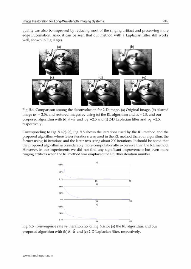
Image Restoration for Long-Wavelength Imaging Systems
249
quality can also be improved by reducing most of the ringing artifact and preserving more edge information. Also, it can be seen that our method with a Laplacian filter still works well, shown in Fig. 5.4(e).
(a) (b)
(c) (d) (e)
Fig. 5.4. Comparison among the deconvolution for 2-D image. (a) Original image, (b) blurred image (σh = 2.5), and restored images by using (c) the RL algorithm and σh = 2.5, and our proposed algorithm with (d) ├ – h and
h =2.5 and (f) 2-D Laplacian filter and
h =2.5,
respectively.
Corresponding to Fig. 5.4(c)-(e), Fig. 5.5 shows the iterations used by the RL method and the proposed algorithm where fewer iterations was used in the RL method than our algorithm, the former using 46 iterations and the latter two using about 200 iterations. It should be noted that the proposed algorithm is considerably more computationally expensive than the RL method. However, in our experiments we did not find any significant improvement but even more ringing artifacts when the RL method was employed for a further iteration number.
25 500 %
50 %
100%(a)
100 2000%
50%
100%(b)
100 2000 %
50%
100%(c)
Fig. 5.5. Convergence rate vs. iteration no. of Fig. 5.4 for (a) the RL algorithm, and our
proposed algorithm with (b) ├ – h and (c) 2-D Laplacian filter, respectively.
www.intechopen.com

Image Restoration – Recent Advances and Applications
250
For further inspection into our proposed algorithm, we investigated the effect of this algorithm using the high pass filter, ├- h , with varied
h . Figure 5.6 demonstrates this case
where the original and the noisy (σh = 2.5 and BSNR=30 dB) images are displayed in Fig. 5.6(a), (b), and the restored images are shown in Fig. 5.6(c)–(e) obtained with the use of
h
equal to 2, 2.5, and 3, respectively. The MSEs of these results are 163.77, 76.82, and 97.97, respectively. Of all the restored images, Fig. 5.6(c) shows a worse image quality than the others, in which noise was intensively produced and hard to be removed although the contrast of the restored image was enhanced. Figure 5.6(d) and (e) show the promising results where high contrast was generated and noise was suppressed. As a result, it is recommended that a small
h~ , together with adequate iterations, should be avoided to use
in the restoration process of the proposed algorithm.
(a) (b)
(c) (d) (e)
Fig. 5.6. Demonstration of the deconvolution for a 2-D image using the proposed algorithm. (a) Original image, (b) noisy image (σh = 2.5 and BSNR=30 dB), and restored images by using our proposed algorithm incorporating ├ – h with (c)
h = 2, (d)
h = 2.5 and (f)
h = 3,
respectively.
5.1.2 Results for a real degraded image
It is always expected that a novel algorithm can be implemented on a real image; Fig. 5.7(a) presents a real degraded image captured by an mm-wave imaging system. Figure 5.7(b) was restored using the RL method and Fig. 5.7(c), (d) were obtained by using our proposed method where Fig. 5.7(b)-(d) were obtained with
,h h equal to 3. It is obvious that the restored
images, Fig. 5.7(c) reveals sharp edges, high contrast and much more details like a number 2, two cars, and three lamps of the floodlight, etc., but Fig. 5.7(b) has shown ringing artifact spreading through the whole image. Furthermore, it is worth mentioning that Fig. 5.7(d) also shows a good image quality which was achieved with the use of a 3 × 3 Laplacian operator.
Corresponding to Fig. 5.7(c)-(e), Fig. 5.8 shows the iterations used by the RL method and the proposed algorithm satisfying with the stopping criterion. In the case of 2-D image, the RL method used less iteration than our algorithm, the former using 35 iterations and the latter two using about 150 iterations.
www.intechopen.com

Image Restoration for Long-Wavelength Imaging Systems
251
(a) (b)
(c) (d)
Fig. 5.7. Comparison among image deconvolution for a 94 GHz millimeter-wave image. (a) Real degraded image, and restored images by using (b) the RL algorithm and σh =3, and our proposed algorithm with (c) ├ – h and
h =3 and (d) 2-D Laplacian filter and
h =3,
respectively.
20 400 %
50%
100%(a)
80 1600%
50%
100%(b)
80 1600%
50%
100%(c)
Fig. 5.8. Convergence rate vs. iteration no. of Fig. 5.7 for (a) the RL algorithm, and our
proposed algorithm with (b) ├ – h and (c) 2-D Laplacian filter, respectively.
www.intechopen.com

Image Restoration – Recent Advances and Applications
252
5.2 Inter-processing: Application to near infrared diffuse optical tomography
5.2.1 Rapid convergence algorithm applied to NIR DOT
Corresponding to Eq. (4.14), some parameters are chosen as
0.75max{ }TJ J , 0
2( ) I , 22.5 nn or e , (5.2)
where the subscript n is the n-th iteration, “max” means the maximum value, and the superscript T denotes a transposition operation. One way to improve the convergence rate is using n as the Type-1 soft prior and using 22.5 n
n e , an exponentially decreasing form, as the Type-2 soft prior, where Type-1 is a parameter related to the system function (Jacobian matrix) and Type-2 is a user-defined parameter. Both values of n have been respectively employed to seek an inverse solution for comparison.
0
0.05
0.1
0 3600
0.05
0.1
(g)
0
0.05
0.1
0 3600
0.05
0.1
(h)
0
0.05
0.1
0 3600
0.05
0.1
(i)
0 10 20 300
0.005
0.01Convergence Rate
iteration no.
MS
E(%
)
0 10 20 300
0.005
0.01Convergence Rate
iteration no.
MS
E(%
)
0 10 20 300
0.005
0.01Convergence Rate
iteration no.
MS
E(%
)
0
0.05
0.1
0 3600
0.05
0.1
(j)
0
0.05
0.1
0 3600
0.05
0.1
(k)
0
0.05
0.1
0 3600
0.05
0.1
(l)
2 incls.3 incls.
2 incls.3 incls.
2 incls.3 incls.
(a) (b) (c)
(d) (e) (f)
(o)(n)(m)
Fig. 5.9. Reconstruction data through various priors with intensity signals corrupted by Gaussian white noise (SNR=20 dB). Left column: constrained inverse solution with soft prior 1; middle column: constrained inverse solution with soft prior 2; right column: constrained inverse solution with hard prior.
Figure 5.9 illustrates the comparisons between constrained solutions using soft priors (Type 1 and 2) and a hard prior, where the left, middle and right columns are the constrained inverse solutions with soft prior 1, soft prior 2, and hard prior [M.-Cheng & M.-Chun Pan, 2010], respectively. Figure 5.9 (a-f) shows the 2D reconstructions of phantoms with two and three inclusions, where slight discrepancy can be observed. Figure 5.9 (g-l) depicts their
www.intechopen.com

Image Restoration for Long-Wavelength Imaging Systems
253
corresponding 1D circular transection profiles to reveal noticeable differences. Basically, there is a better separation resolution but a lower intensity owing to a highly suppressed signal by a hard prior rather than a soft prior. Additionally, Fig. 5.9 (m-o) exhibits good convergences obtained by using both soft and hard priors.
5.2.2 Image restoration applied to NIR DOT
The phantoms employed for justifying our proposed technique (Sec. 3.4) incorporate two or three inclusions with various sizes, locations and separations, illustrated in Fig. 5.10, where R denotes radius in the unit of mm. Of the phantom, the background absorption (┤a) and reduced scattering (┤’s ) values are about 0.0025 mm-1 and 0.25 mm-1, respectively, while the maximum absorption and reduced scattering for the inclusion are 0.025 mm-1 and 2.5 mm-1, thereby assuming the contrast ratio of the inclusion to background 10:1, because high contrast results in much more overlapping effects than low contrast although a contrast of 2~10 were used throughout other published works.
(a) (b)
Fig. 5.10. Schematic diagram for the dimensions of two different test cases in simulation. (a) and (b) are Case 1, 2, respectively, where R is radius in the unit of mm.
As depicted in Fig. 5.10, Case 1, 2, respectively, have two inclusions separated with a similar distance but different sizes. As the separation resolution of inclusions is examined, several (two or three) embedded inclusions are necessary, and different inclusion sizes are considered as well. For the convenience in discussion latter, we denote M0-4 as the reconstructions with the schemes using non-filtering, ├-g2 (σ2=1.5), g1-g2(σ1=0.75, σ2=1.5), wavelet (a dilated factor a=0.5), and Laplacian high-pass filter (HPF) in their 2D form, respectively. Currently, absorption-coefficient images are presented for our continuous wave image reconstruction algorithm.
In FEM-based image reconstruction, the homogeneous background (┤a = 0.0025mm-1, ┤’s = 0.25mm-1) was adopted as an initial guess. Thirty-iteration assignment was employed for
each case as the normalized increasing rate, i.e. mean value of 2
1n n
n
, reaches smaller
than 10-2.
www.intechopen.com

Image Restoration – Recent Advances and Applications
254
5.2.3 Examples illustration
5.2.3.1 Case 1
This case was designed as a phantom with three smaller inclusions. Several improved images were obtained by using appropriate filtering, as shown in Fig. 5.11(b-e) of 1D circular profiles passing through the centers of inclusions. Likewise, M2 resulted in worse resolved image than others with HP filtering. Negative artifacts occurred in each reconstructed image, as depicted in Fig. 5.11(g-j). It is well noted that M4 overestimated the inclusion amplitudes, which yields a higher inclusion-to-background contrast.
0 180 3600
0.01
0.02
(f)
Degree
Absorp
tion c
oeff
icie
nt
(mm
-1)
(b)
0
0.01
0.02
0 180 3600
0.01
0.02
(g)
Degree
0 180 3600
0.01
0.02
(h)
Degree
(c)
0
0.01
0.02
(d)
0
0.01
0.02
0 180 3600
0.01
0.02
(i)
Degree
(a)
0
0.01
0.02
(e)
0
0.01
0.02
0 180 3600
0.01
0.02
(j)
Degree Fig. 5.11. Case 1- 2D reconstructed absorption images (a) without HPF (M0) and (b)-(e) with M1, M2, M3, M4 filtering, respectively; (f)-(j) are 1D circular profiles corresponding to (a)-(e), where solid lines are the designed, and dotted lines represent the reconstructed.
5.2.3.2 Case 2
In this highly challenging case, a phantom with two closest-separation inclusions was designed. As shown in Fig. 5.12(a-e), all reconstructed images underestimated inclusions, and offered relatively bad resolution for two separate inclusions. It is rather competitive for these employed filters. Based upon a quantitative comparison, as depicted in Fig. 5.12(i) and (j), M3 and M4 schemes demonstrate better resolution discrimination to separate bigger and closer inclusions in comparison of Case 1.
From the results of Case 1 and 2 for a phantom with inclusions of both small size and close separation, it can be concluded that the wavelet-like HP filtering (M3) demonstrates the best spatial-frequency resolution capability to the inclusions.
It evidently shows that the enhancement of reconstruction through the incorporation of our proposed HPF approach can effectively improve computed images. As illustrated above, the wavelet-like HP filtering schemes (M3, M4) further yields better results than the LPF-combined HP filtering schemes (M1, M2). In the aspects of sensitivity and stability of evaluation, M3 yielded results closest to the true absorption property than other schemes. However, M4 visually characterizes the inclusion-to-background contrast best.
www.intechopen.com

Image Restoration for Long-Wavelength Imaging Systems
255
0 180 3600
0.01
0.02
(f)
Degree
Absorp
tion c
oeff
icie
nt
(mm
-1)
(b)
0
0.01
0.02
0 180 3600
0.01
0.02
(g)
Degree
(c)
0
0.01
0.02
0 180 3600
0.01
0.02
(h)
Degree
(d)
0
0.01
0.02
0 180 3600
0.01
0.02
(i)
Degree
(a)
0
0.01
0.02
(e)
0
0.01
0.02
0 180 3600
0.01
0.02
(j)
Degree Fig. 5.12. Case 2- 2D reconstructed absorption images (a) without HPF (M0) and (b)-(e) with M1, M2, M3, M4 filtering, respectively; (f)-(j) are 1D circular profiles corresponding to (a)-(e), where solid lines are the designed, and dotted lines represent the reconstructed.
5.2.4 Performance investigation
In terms of the optical properties within the inclusion and background, it is worth noted that the image reconstruction is not only pursuing qualitative correctness but also obtaining favorably quantitative information about the optical properties of either the inclusions or background. Parameters of interest such as size, contrast and location variations associated image quantification measures are most frequently investigated and discussed. Readers can refer to the research work [Pan et al., 2008].
5.3 Remark
In this section, we have demonstrated the performance of our proposed image restoration algorithms exactly applied in the imaging process for ‘inter-processing’ and to corrupted images for ‘post-processing.’
6. Conclusions
6.1 Concluding remark
In this chapter, we have explained the background and the mathematical model of image formation and image restoration for long-wavelength imaging systems; as well, image restoration algorithms, further consideration on image restoration, and their related application have been described and demonstrated. In the meanwhile, a promising method to restore images has been proposed. As discussed in this chapter, the proposed algorithm was applied to both simulated and real atmospherically degraded images. Restoration results show significantly improved images. Especially, the restored millimeter-wave image highlights the superior performance of the proposed method in reality. The main novelty here is that error energy resulting from noise and ringing artifact is highly suppressed with
www.intechopen.com

Image Restoration – Recent Advances and Applications
256
the algorithm proposed in this chapter. Also, we have used such a resolution-enhancing technique with HP filtering incorporated with the FEM-based inverse computation to obtain highly resolved tomographic images of optical-property.
In addition, we have developed and realized the schemes for expediting NIR DOT image reconstruction through the inverse solution regularized with the constraint of a Lorentzian distributed function. Substantial improvements in reconstruction have been achieved without incurring additional hardware cost. With the introduction of constraints having a form of the Lorentzian distributed function, rapid convergence can be achieved owing to the fact that decreasing Δχ results in the increase of ┣ as the iteration process proceeds, and vice versa. It behaves like a criterion in the sense of a rapid convergence that the optimal iteration number is founded as seeking an inverse solution regularized with the Lorentzian distributed function.
6.2 Future work
It is anticipated that of regularizing mean square error (residual term) with error energy reduction and rapid convergence (a priori terms) an algorithm is explored to restore images effectively and efficiently. In addition, it is no doubt that image restoration for inter-discipline application is the focus in the future research.
7. Acknowledgements
In collaboration with the DASD laboratory at the Department of Mechanical Engineering of National Central University, the author wish to thank group leader and members to develop the software (NIR.FD_PC) and validate the instrumentation for NIR DOT imaging system. Also, the author would like to acknowledge the funding support from the grants by the National Science Council (NSC 93-2213-E-236-002, NSC 95-2221-E-236-002, NSC 98-2221-E-236-013, NSC 99-2221-E-236-014, NSC 100-2221-E-236-012) in Taiwan (ROC).
8. References
[1] Archer, G. & Titterington, D. M. (1995). On Some Bayesian/Regularization Methods for Image Restoration. IEEE Trans. on Image Processing, Vol. 4, pp. 307-310
[2] Brendel, B. & Nielsen, T. (2009). Selection of Optimal Wavelengths for Spectral Reconstruction in Diffuse Optical Tomography. Journal of Biomedical Optics, Vol. 14, 034041
[3] Chen, W.; Chen, M. & Zhou, J. (2000). Adaptively Regularized Constrained Total Least-Squares Image Restoration. IEEE Trans. on Image Processing, Vol. 9, pp. 588-596
[4] Davis, S. C.; Dehghani, H.; Wang, J.; Jiang, S.; Pogue, B. W. & Paulsen, K. D. (2007). Image-guided Diffuse Optical Fluorescence Tomography Implemented with Laplacian-type Regularization. Opt. Exp. , Vol. 15, pp. 4066-4082
[5] Frieden, B. R. (1972). Restoring with Maximum Likelihood and Maximum Entropy, J. Opt. Soc. Am., Vol. 62, pp. 511-518
[6] Gerchberg, R. W. (1974). Super-Resolution through Error Energy Reduction. Opt. Acta, Vol. 21, pp. 709-720
www.intechopen.com

Image Restoration for Long-Wavelength Imaging Systems
257
[7] Gillette, J. C.; Stadtmiller, T. M. & Hardie, R. C. (1995). Aliasing Reduction in Staring Infrared Imagers Utilizing Subpixel Techniques. Opt. Eng., Vol. 34, pp. 3130-3137
[8] Holboke, M. J.; Tromberg, B. J.; Li, X.; Shah, N.; Fishkin, J.; Kidney, D.; Butler, J.; Chance, B. & Yodh, A. G. (2000). Three-dimensional Diffuse Optical Mammography with Ultrasound Localization in a Human Subject. Journal of Biomedical Optics, Vol. 5, pp. 237-247
[9] Hou, H. & Andrews, H. (1978). Cubic Splines for Image Interpolation and Digital Filtering. IEEE Transactions on Acoustics, Speech, and Signal Processing, Vol. 26, No. 6, pp. 508–517
[10] Hunt, B. R. & Sementilli, P. J. (1992). Description of a Poisson Imagery Superresolution Algorithm, Astronomical Data Analysis Software and System I., A.S.P. Conf. Ser. , Vol. 25, pp. 196-199
[11] Hunt, B. R. (1994). Prospects for Image Restoration, Int. J. Mod. Phys., C 5, pp. 151-178 [12] Jain, A. K. (1989).Fundamentals of Digital image Processing, Prentice- Hall, Englewood
Cliffs, NJ, USA [13] Keys, R. (1981). Cubic Convolution Interpolation for Digital Image Processing. IEEE
Transactions on Acoustics, Speech, and Signal Processing, Vol. 29, No. 6, pp. 1153–1160 [14] Kundur, D. & Hatzinakos, D. A (1998). Novel Blind Deconvolution Scheme for Image
Restoration Using Recursive Filtering. IEEE Transactions on Signal Processing, Vol. 46, No. 2, pp375-390
[15] Landi, G. (2007). A Fast Truncated Lagrange Method for Large-Scale Image Restoration Problems, Applied Mathematics and Computation, Vol. 186, pp. 1075–1082.
[16] Lettington, A. H. & Hong, Q. H. (1995). Image Restoration Using a Lorentzian Probability Model. J. Mod. Opt. , Vol. 42, pp. 1367-1376
[17] Lucy, L. B. (1974). An Iterative Technique for the Rectification of Observed Distributions. The Astron. J., Vol. 79, pp. 745-765
[18] Meinel, E. S. (1986). Origins of Linear and Nonlinear Recursive Restoration Algorithms. J. Opt. Soc. Am., A 3, pp. 787-799
[19] Ng, M. K.; Molina, R. & Bose, N. K. (2003). Mathematical Analysis of Super-Resolution Methodology, IEEE Signal Processing Mag. , Vol. 20, pp. 62-74
[20] Pan, M. C. & Lettington, A. H. (1998). Smoothing Images by a Probability Filter. Proc. IEEE International Joint Symposia on Intelligence and Systems, pp.343-346.
[21] Pan, M. C. & Lettington, A. H. (1999). Efficient Method for Improving Poisson MAP Super-resolution. Electronics Letters, Vol. 35, No. 10, pp. 803-805
[22] Pan, M. C. (2003). A Novel Blind Super-resolution Algorithm for Restoring Gaussian Blurred Images. The International Journal of Imaging Systems & Technology, Vol. 12, pp. 239-246
[23] Pan, M. C. (2006). Improving a Single Down-sampled Image Using Probability -filtering-based Interpolation and Improved Poisson Maximum a posteriori Super-resolution. EURASIP Journal on Applied Signal Processing, Vol. 2006, Article ID 97492 (1-9)
[24] Pan, M.-Cheng; Chen, C. H.; Chen, L.Y.; Pan, M.-Chun & Shyr, Y. M. (2008). Highly-resolved Diffuse Optical Tomography: A Systematical Approach Using High-pass Filtering for Value-preserved Images. Journal of Biomedical Optics, Vol. 13, No. 02, pp. Article ID 024022 (1-14)
www.intechopen.com

Image Restoration – Recent Advances and Applications
258
[25] Pan, M.-Cheng & Pan, M.-Chun (2010). Rapid Convergence to the Inverse Solution Regularized with the Lorentzian Distributed Function for Near-infrared Continuous Wave Diffuse Optical Tomography,” Journal of Biomedical Optics, Vol. 15, 016014(1-11)
[26] Pan, M. C. (2010). Image Restoration Through Regularization Based on Error Energy Minimization. International Journal of Imaging Systems & Technology, Vol. 20, No. 4, pp. 308-315
[27] Paulsen, K. D. & Jiang, H. (1995). Spatially Varying Optical Property Reconstruction Using a Finite Element Diffusion Equation Approximation. Med. Phys., Vol. 22, pp. 691-701
[28] Pogue, B. W.; McBride, T. O.; Prewitt, J.; Österberg, U. L. & Paulsen, K. D. (1999). Spatially Variant Regularization Improves Diffuse Optical Tomography. Appl. Opt., Vol. 38, pp. 2950-2961
[29] Richardson, W. H. (1972). Bayesian-based Iterative Method of Image Restoration. J. Opt. Soc. Am., Vol. 62, pp. 55-59
[30] Segal, C.; Molina, R. & Katsaggelos, K. (2003). High-resolution Images from Low-Resolution Compressed Video. IEEE Signal Processing Mag. , Vol. 20, pp. 37-48
[31] Sezan, M. I. & Tekalp, A. M. (1988). Iterative Image Restoration with Ringing Suppression Using POCS. Proceedings of IEEE Int. Conf. Acoust., Speech, Signals Processing, pp. 1300-1303
[32] Singh, S.; Tandon, S. N. & Gupta, H. M. (1986). An Iterative Restoration Technique. Signal Processing, Vol. 11, pp. 1-11
[33] Stewart, K. & Durrani, T. S. (1986). Constrained Signal Reconstruction--A Unified Approach. EURASIP Signal Processing III, pp. 1423-1426
[34] Teboul, S.; Blanc-Feraud, L.; Aubert, G. & Barlaud, M. (1998). Variational Approach for Edge-Preserving Regularization Using Coupled PDE’s. IEEE Transactions on Image Processing, Vol. 7, pp. 387-397
[35] Toraldo di Francia, G. (1952). Supergain Antennas and Optical Resolving Power. Nuovo Cimento Suppl, Vol. 9, pp. 426-435
[36] Toraldo di Francia, G. (1955). Resolving Power and Information. J. Opt. Soc. Am. , Vol. 45, pp. 497-501
[37] Wiener, N. (1942). Extrapolation, Interpolation, and Smoothing of Stationary Time Series, MIT Press, USA
www.intechopen.com

Image Restoration - Recent Advances and ApplicationsEdited by Dr Aymeric Histace
ISBN 978-953-51-0388-2Hard cover, 372 pagesPublisher InTechPublished online 04, April, 2012Published in print edition April, 2012
InTech EuropeUniversity Campus STeP Ri Slavka Krautzeka 83/A 51000 Rijeka, Croatia Phone: +385 (51) 770 447 Fax: +385 (51) 686 166www.intechopen.com
InTech ChinaUnit 405, Office Block, Hotel Equatorial Shanghai No.65, Yan An Road (West), Shanghai, 200040, China
Phone: +86-21-62489820 Fax: +86-21-62489821
This book represents a sample of recent contributions of researchers all around the world in the field of imagerestoration. The book consists of 15 chapters organized in three main sections (Theory, Applications,Interdisciplinarity). Topics cover some different aspects of the theory of image restoration, but this book is alsoan occasion to highlight some new topics of research related to the emergence of some original imagingdevices. From this arise some real challenging problems related to image reconstruction/restoration that openthe way to some new fundamental scientific questions closely related with the world we interact with.
How to referenceIn order to correctly reference this scholarly work, feel free to copy and paste the following:
Min-Cheng Pan (2012). Image Restoration for Long-Wavelength Imaging Systems, Image Restoration -Recent Advances and Applications, Dr Aymeric Histace (Ed.), ISBN: 978-953-51-0388-2, InTech, Availablefrom: http://www.intechopen.com/books/image-restoration-recent-advances-and-applications/image-restoration-for-long-wavelength-imaging-system

© 2012 The Author(s). Licensee IntechOpen. This is an open access articledistributed under the terms of the Creative Commons Attribution 3.0License, which permits unrestricted use, distribution, and reproduction inany medium, provided the original work is properly cited.