General rights Copyright and moral rights for the publications made accessible in the public portal are retained by the authors and/or other copyright owners and it is a condition of accessing publications that users recognise and abide by the legal requirements associated with these rights.

• Users may download and print one copy of any publication from the public portal for the purpose of private study or research. • You may not further distribute the material or use it for any profit-making activity or commercial gain • You may freely distribute the URL identifying the publication in the public portal

If you believe that this document breaches copyright please contact us providing details, and we will remove access to the work immediately and investigate your claim.

Downloaded from orbit.dtu.dk on: Oct 12, 2018

Image Registration and Optimization in the Virtual Slaughterhouse

Vester-Christensen, Martin; Larsen, Rasmus; Christensen, Lars Bager

Publication date:2009

Document VersionPublisher's PDF, also known as Version of record

Link back to DTU Orbit

Citation (APA):Vester-Christensen, M., Larsen, R., & Christensen, L. B. (2009). Image Registration and Optimization in theVirtual Slaughterhouse. Kgs. Lyngby, Denmark: Technical University of Denmark (DTU). IMM-PHD-2008-206

Image Registration andOptimization in the Virtual

Slaughterhouse

Martin Vester-Christensen

Kongens Lyngby 2008

IMM-PHD-2008-206

Technical University of Denmark

Department of Informatics and Mathematical Modeling

Building 321, DK-2800 Kongens Lyngby, Denmark

Phone +45 45253351, Fax +45 45882673

reception@imm.dtu.dk

www.imm.dtu.dk

IMM-PHD: ISSN 0909-3192

Preface

This thesis was prepared at the Image Analysis and Computer Graphics groupat DTU Informatics and submitted to the Technical University of Denmark- DTU, in partial fulfilment of the requirements for the degree of Doctor ofPhilosophy, Ph.D., in Applied Mathematics. The project was funded by DTU,Danish Meat Association and the Danish Technical Research Council.

The work herein represents selected parts of the research work carried out inthe Ph.D. period. The thesis consists of an introductory, a theoretical part andthree research papers.

The work was carried out in a close collaboration with the Danish Meat ResearchInstitute of the Danish Meat Association at the institute in Roskilde, Denmark.Part of the research was conducted at Institut fur Mathematik, Universitat zuLubeck, Lubeck, Germany. The project was supervised by Professor RasmusLarsen - DTU Informatics and Ph.D. Lars Bager Christensen - Danish MeatResearch Institute.

Kgs. Lyngby, October 2008

Martin Vester-Christensen

ii

Acknowledgements

This thesis is the product of a collective effort of many people. Each of playingan important role in its completion.

First and foremost my deepest gratitude and respect goes to my supervisorProfessor Rasmus Larsen. For accepting me as a Ph.D.-student ”back in theday” but also for the whole process of maturing me as a student and person.

The great people at the Danish Meat Research Institute in Roskilde, Denmark.A more open-minded and innovative place is hard to find. I owe an immensedebt of gratitude to all the good people there. The willingness to immediatelyconcentrate 100% on my problems has been incredible. The enormous interestin the project has been overwhelming and at times the principal reason for itscontinuation. Lars Bager Christensen for being a great mentor, innovator andfriend. His immense contribution and support is greatly appreciated. Eli V.Olsen for continuously promoting my work and her unconditional support. Forintroducing me to the many aspects of the pig slaughtering business and showingme the bigger picture. Marchen Hviid for her many contributions, her drive andcontinued belief in the project. I thank Claus Borggaard, Jesper Blom-Hansenand Niels-Christian Kjærsgaard and many others for great collaboration duringthe project.

My great friends and colleagues Søren Gylling Hemmingsen Erbou and MadsFogtmann Hansen. We have truly been comrades in arms. The three yearswould not have been the same without them.

This Ph.d. project was not half the fun without my great colleagues amongst thestaff and Ph.d.-students at the Image Analysis and Computer Graphics groupIMM,DTU. Honorable mentions are Sune Darkner for being an exceptional col-

iv Acknowledgements

leagues and friend and my office mate Michael Sass Hansen for patiently puttingup with the ramblings of a grumpy ”old” man. A special thanks goes to Einaand Tove for making the practical issues easy.

The SAFIR group headed by Professor Bernd Fischer at Institut fur Math-ematik, Universitat zu Lubeck for allowing me stay with them for two veryfunny months in May and June 2007. A truly heartfelt thank you goes to Dr.Jan Modersitzki for accepting me with kindness and friendliness both in Lubeckand in Canada. For sharing of his enormous knowledge and for the patienceduring my tutoring. That was truly above and beyond the call of duty.

Finally, I extend my love and gratitude to my wife Malene for her complete sup-port and understanding throughout the period. Especially for making my stayin Lubeck possible by being a single-mom for two long months. My daughtersMille and Mathilde for always reminding me of the really important things inlife.

Abstract

This thesis presents the development and application of algorithms for the anal-ysis of pig carcasses. Focus is on the simulation and quality estimation of meatproducts produced in a Danish slaughterhouse. Computed Tomography scans ofpig carcasses provide the data used in the application. Image analysis is appliedin order to imitate some of the cutting processes found in a slaughterhouse butalso to give a quantitative measure of the composition of each carcass.

The basis of the algorithms is non-linear image registration. This method findsthe anatomical correspondence between a reference carcass and a template car-cass. By iteratively comparing the transformed template with the reference aresulting dense deformation field is found. Propagating a set of landmarks fromthe reference coordinate system onto the template enables the simulation ofslaughtering processes.

Non-invasively estimating the quality of the slaughtering products provides avery valuable tool for use in the slaughterhouse in the future.

vi

Resume

Denne afhandling beskriver udviklingen og anvendelsen af algoritmer til analyseaf svineslagtekroppe. Der fokuseres specielt pa simulering og kvalitetsbestem-melse af kød produkter produceret pa et dansk slagteri. Computer Tomografiskanning af slagtekroppe udgør data brugt i applikationen. Billedanalyse er an-vendt for at efterligne udskæringsprocessen, men ogsa til at give et kvantitativtmal for sammensætningen af de enkelte slagtekroppe.

Algoritmerne er baseret pa ikke-lineær billedregistrering. Denne metode finderanatomisk korrespondance mellem en reference slagtekrop og en test slagtekrop.Ved iterativt at sammenligne den transformerede test slagtekrop med referencenfindes et resulterende deformationsfelt. Ved at transmittere en række referen-cepunkter fra reference slagtekroppen til test slagtekroppe muliggøres simulerin-gen af slagteprocessen.

Ikke-invasiv estimering af kvaliteten af slagteprodukter udgør et meget værdi-fuldt værktøj til brug i slagterierne i fremtiden.

viii

List of Published Papers

Listed here are peer-reviewed scientific papers and abstracts prepared duringthe course of the Ph.D. program. The papers included in this thesis is markedwith bold typeface of the title.

Journal papers:

• M. Vester-Christensen, S. G. H. Erbou, M. F. Hansen, E. V. Olsen, L. B.Christensen, M. Hviid, B. K. Ersbøll, R. Larsen Virtual Dissection of

Pig Carcasses. Meat Science, 2008. Submitted.

• S. G. H. Erbou, M. Vester-Christensen, R. Larsen, L. B. Christensen, B.K. Ersbøll. Sparse 3D shape modelling of bone structures Machine Vision

and Applications, 2008. Submitted.

Conference papers:

• M. Hviid, M. Vester-Christensen. Density of lean meat tissue in pork -measured by CT. 54th International Congress of Meat Science and Tech-

nology - ICoMST, 2008.

• L. B. Christensen, M. Vester-Christensen, C. Borggaard, E. V. Olsen. Ro-

bustness of weight and meat content in pigs determined by CT.54th International Congress of Meat Science and Technology - ICoMST,2008.

• S. Darkner, M. Vester-Christensen, R.R. Paulsen, R.Larsen. Non-rigidsurface registration of 2D manifolds in 3D Euclidian space. International

Symposium on Medical Imaging - SPIE, 2008.

x

• M. F. Hansen, S. G. H. Erbou, M. Vester-Christensen, R. Larsen, L. B.Christensen. Surface-to-surface registration using level sets. ScandinavianConference on Image Analysis - SCIA, 2007.

• M. Vester-Christensen , S. G. H. Erbou, S. Darkner, R. Larsen. Accel-

erated 3D image registration. International Symposium on Medical

Imaging - SPIE, 2007.

• S. Darkner, M. Vester-Christensen, R. Larsen. Evaluating a methodfor automated rigid registration. International Symposium on Medical

Imaging - SPIE, 2007.

• S. Darkner, M. Vester-Christensen, R. Larsen, C. Nielsen, R. R. Paulsen.Automated 3D Rigid Registration of Open 2D Manifolds. From Statistical

Atlases to Personalized Models - MICCAI 2006 Workshop, 2006.

• A. Lyckegaard, R. Larsen, L. B. Christensen, M. Vester-Christensen, E.V. Olsen. Contextual Analysis of CT Scanned Pig Carcasses. 52nd

International Congress of Meat Science and Technology - ICoMST, 2006.

Abstracts:

• M. Vester-Christensen, R. Larsen. Atlas Construction using Fast ImageRegistration. Image Analysis in Vivo Pharmachology - IAVP, 2007.

• S. G. H. Erbou, M. Vester-Christensen, R. Larsen, E. V. Olsen, B. K.Ersbøll. Quantifying Biological Variation. European Congress of Chemi-

cal Engineering - ECCE6 - Special Symposium - Innovations in Food Tech-

nology, 2007.

xi

xii Contents

Contents

Preface i

Acknowledgements iii

Abstract v

Resume vii

List of Published Papers ix

Contents xiii

I The Virtual Slaughterhouse 1

1 Introduction 3

1.1 Thesis Objective . . . . . . . . . . . . . . . . . . . . . . . . . . . 4

1.2 Thesis Overview . . . . . . . . . . . . . . . . . . . . . . . . . . . 4

2 CT in the Meat Industry 7

xiv CONTENTS

2.1 The Danish Meat Industry . . . . . . . . . . . . . . . . . . . . . . 7

2.2 Pig Carcass Classification - The Lean Meat Percentage . . . . . . 11

2.3 Previous Work and Applications . . . . . . . . . . . . . . . . . . 12

2.4 The Virtual Slaughterhouse . . . . . . . . . . . . . . . . . . . . . 12

3 Imaging 15

3.1 Half Carcasses . . . . . . . . . . . . . . . . . . . . . . . . . . . . 15

3.2 Computed Tomography 101 . . . . . . . . . . . . . . . . . . . . . 16

3.3 Image Data . . . . . . . . . . . . . . . . . . . . . . . . . . . . . . 16

3.4 Anatomical Landmarks . . . . . . . . . . . . . . . . . . . . . . . 23

II Algorithms for Image Registration 25

4 Introduction 27

4.1 Algorithms and Applications . . . . . . . . . . . . . . . . . . . . 28

5 Images and Image Transformation 31

5.1 Images . . . . . . . . . . . . . . . . . . . . . . . . . . . . . . . . . 31

5.2 Image Transformations . . . . . . . . . . . . . . . . . . . . . . . . 34

5.3 Affine Transformations . . . . . . . . . . . . . . . . . . . . . . . . 36

5.4 B-Spline Transformations . . . . . . . . . . . . . . . . . . . . . . 38

6 Image Registration - a Large Scale Optimization Problem 41

6.1 Similarity Measurements . . . . . . . . . . . . . . . . . . . . . . . 41

6.2 The Gauss-Newton Method . . . . . . . . . . . . . . . . . . . . . 43

6.3 Step Length . . . . . . . . . . . . . . . . . . . . . . . . . . . . . . 44

6.4 Solving the Linear Problem . . . . . . . . . . . . . . . . . . . . . 47

CONTENTS xv

6.5 Regularization . . . . . . . . . . . . . . . . . . . . . . . . . . . . 51

6.6 Parametric Image Registration Algorithm . . . . . . . . . . . . . 54

6.7 Evaluation of Image Registration . . . . . . . . . . . . . . . . . . 56

III Applications 59

7 Virtual Jointing of Pig Carcasses using Image Registration 61

7.1 Introduction . . . . . . . . . . . . . . . . . . . . . . . . . . . . . . 62

7.2 The Data . . . . . . . . . . . . . . . . . . . . . . . . . . . . . . . 64

7.3 Image Registration . . . . . . . . . . . . . . . . . . . . . . . . . . 64

7.4 Atlas Construction . . . . . . . . . . . . . . . . . . . . . . . . . . 68

7.5 Virtual Jointing . . . . . . . . . . . . . . . . . . . . . . . . . . . . 69

7.6 Yield Prediction Models . . . . . . . . . . . . . . . . . . . . . . . 76

7.7 Results . . . . . . . . . . . . . . . . . . . . . . . . . . . . . . . . . 79

7.8 Discussion and Conclusion . . . . . . . . . . . . . . . . . . . . . . 84

7.9 Appendix . . . . . . . . . . . . . . . . . . . . . . . . . . . . . . . 85

IV Contributions 91

8 Robustness of weight and meat content in pigs determined by

CT 93

8.1 Introduction . . . . . . . . . . . . . . . . . . . . . . . . . . . . . . 94

8.2 Material and Methods . . . . . . . . . . . . . . . . . . . . . . . . 94

8.3 Results and Discussions . . . . . . . . . . . . . . . . . . . . . . . 95

8.4 Conclusion . . . . . . . . . . . . . . . . . . . . . . . . . . . . . . 97

8.5 Acknowledgements . . . . . . . . . . . . . . . . . . . . . . . . . . 99

xvi CONTENTS

9 Virtual Dissection of Pig Carcasses 101

9.1 Introduction . . . . . . . . . . . . . . . . . . . . . . . . . . . . . . 101

9.2 Materials and Methods . . . . . . . . . . . . . . . . . . . . . . . . 104

9.3 Results and Discussion . . . . . . . . . . . . . . . . . . . . . . . . 108

9.4 Conclusions . . . . . . . . . . . . . . . . . . . . . . . . . . . . . . 113

10 Accelerated 3D Image Registration 115

10.1 Introduction . . . . . . . . . . . . . . . . . . . . . . . . . . . . . . 116

10.2 Methods . . . . . . . . . . . . . . . . . . . . . . . . . . . . . . . . 117

10.3 Results . . . . . . . . . . . . . . . . . . . . . . . . . . . . . . . . . 126

10.4 Conclusion . . . . . . . . . . . . . . . . . . . . . . . . . . . . . . 130

A Demos 135

A.1 OinkExplorer . . . . . . . . . . . . . . . . . . . . . . . . . . . . . 135

A.2 OinkDemo . . . . . . . . . . . . . . . . . . . . . . . . . . . . . . . 137

List of Tables 140

List of Figures 145

List of Algorithms 147

Bibliography 156

Part I

The Virtual Slaughterhouse

Chapter 1

Introduction

The topic of this thesis is, as the title indicates, about slaughterhouses and theslaughtering of pigs. More specifically simulating the process on a computerthus creating a ”Virtual Slaughterhouse”. A slaughterhouse today is very in-dustrialized and automated. Thousands of pigs are processed each day. Theindividual carcasses can be cut into a variety of different products. Choosingthe right mixture of products for a given carcass is the key to success. How-ever, this decision depends not only on the composition of the carcass but alsoon the incoming orders from the customers of the slaughterhouse. Being liv-ing creatures the pigs are very different anatomically and thus the input intoa slaughterhouse is very inhomogeneous. Knowledge of the individual pig iscrucial in order to maximize profits and at the same time maintain the level ofquality demanded by the customers. The Virtual Slaughterhouse is a tool forproviding this knowledge and the means are Computed Tomography scans ofthe pig carcasses and subsequence image processing.

Computed Tomography(CT) provides an in-vivo view of each carcass, yieldinga very detailed level of information about virtually all anatomical regions of thecarcass. Complete knowledge of the anatomy provides the means to the potentialoptimal decision of the use of the individual carcasses. However, the CT dataneeds to be related to the actual processing of the carcass in the slaughterhouse.Thus, there is need for the Virtual Slaughterhouse.

Slaughtering a pig virtually means cutting a carcass into many products without

4 Introduction

it even seeing a knife. Coupling each of these virtual products with a measureof its quality provides the means of choosing the optimal way to process thecarcass. The task is to create algorithms capable of mimicking the set of cutsand apply them on a population of carcasses. This is the topic of this thesis.

Image registration is the foundation of the algorithms created in this thesis. Itis a well-known discipline used widely in medical imaging and as a consequencemany of the algorithms and methods used in the Virtual Slaughterhouse areborrowed from the medical imaging community and literature. However in thisthesis the purpose of the application of image registration is remarkably differ-ent. A series of virtual cuts are defined in a so-called references carcass. Imageregistration enables the propagation of these cuts onto a population of pigs thusenabling the subsequent quality measure.

1.1 Thesis Objective

As in any real life application of mathematics and computer science knowledgeof the problem domain is required. This work is no exception and it is reflectedin the thesis.

The purpose of this thesis is two-fold. It is a theoretical overview of the math-ematical disciplines involved in performing image registration. The aim is toprovide a more or less self contained guide on the practical implementation ofparametric image registration. On the other hand it gives is an overview of someof the concepts and practices involved in the slaughtering of pigs.

Ultimately it is the goal to describe the Virtual Slaughterhouse for the automaticevaluation of the quality of cuts of meat.

1.2 Thesis Overview

The thesis is divided into four parts.

Part I is the introductory part. It provides the background needed to better un-derstand the problem domain in which the thesis is placed. Chapter 2 describesthe Danish meat industry with emphasis on the pig slaughtering industry andit describes Virtual Slaughterhouse. A review of the kind of data and the dataacquisition is described in chapter 3.

Part II is a theoretical description of the image registration algorithms used.

1.2 Thesis Overview 5

It provides the theoretical background and practical implementation issues in-volved in parametric image registration. Chapter 4 introduces image registra-tion and provides an overview of the literature. In chapter 5 the concept ofimages and image transformation is explained. Chapter 6 contains the bulk ofthe part and describes image registration as a large scale optimization problem.It revolves around the Gauss-Newton algorithm and contains the solution topractical implementation issues such as dealing with the very large matrices.

Part III describes the actual application of the algorithms on carcass data.Chapter 7 is a self-contained description of the algorithms implementing theautomatic quality grading using virtual cuts. It is a demonstration of the powerin applying the use of CT scans and image analysis on a practical problem suchas estimating the quality of certain cuts of meat.

Part IV is a collection of published contributions written during the project.They cover different aspects of the concepts found in the thesis. Chapter 8describes an experiment demonstration the robustness of using the CT as aquantitative measuring tool. The results show that CT offers a robust measure-ment technology with a very small sensitivity to the different settings of thescanning protocol. Chapter 9 describes the creation of a linear model of therelation between voxels and the full weight of the half carcass. This knowledgeenables the determination of the lean meat percentage. The lean meat percent-age is a measure of the quality of the meat in a carcass and used to predict thequality of individual cuts. Chapter 10 describes the creation of an alternativeparametric image registration algorithm than that described in part two.

Finally appendix A contains a view of two of the demonstration programs pro-duced during the project.

6 Introduction

Chapter 2

CT in the Meat Industry

The topics of this thesis are connected to the meat industry. More specificallythe pig slaughtering industry. The Danish slaughterhouses are undergoing achange with the use of advanced technology in the slaughtering process. Inrecent years the use of Computed Tomography(CT) as modeling and measuringtool in connection with the slaughtering of pigs has been investigated. Thisproject is denoted The Virtual Slaughterhouse. The name covers the building ofcomputerized mathematical models of many aspects of the processes going on ina slaughterhouse. Using these models a pig carcass can be virtually slaughteredon a computer before it even sees a knife and the results can be evaluated. Thusproviding some of the building blocks of a decision support system to be usedin the slaughterhouses.

2.1 The Danish Meat Industry

The Danish meat industry is one of the largest and most important industriesin the country, with the pig industry being by far the largest part. The annualexport of pig meat is roughly 30 billion DKK, around 4.0 billion EUR, andrepresents about 5 pct. of the total annual export [114]. As such the story ofthe pig industry is for the most part a story of success. However in recent years,especially 2007 a year with increasing price on feed, the profits have decreased.

8 CT in the Meat Industry

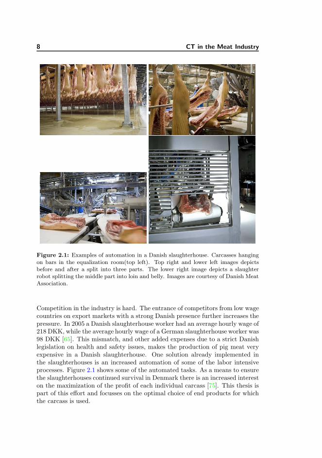
Figure 2.1: Examples of automation in a Danish slaughterhouse. Carcasses hangingon bars in the equalization room(top left). Top right and lower left images depictsbefore and after a split into three parts. The lower right image depicts a slaughterrobot splitting the middle part into loin and belly. Images are courtesy of Danish MeatAssociation.

Competition in the industry is hard. The entrance of competitors from low wagecountries on export markets with a strong Danish presence further increases thepressure. In 2005 a Danish slaughterhouse worker had an average hourly wage of218 DKK, while the average hourly wage of a German slaughterhouse worker was98 DKK [65]. This mismatch, and other added expenses due to a strict Danishlegislation on health and safety issues, makes the production of pig meat veryexpensive in a Danish slaughterhouse. One solution already implemented inthe slaughterhouses is an increased automation of some of the labor intensiveprocesses. Figure 2.1 shows some of the automated tasks. As a means to ensurethe slaughterhouses continued survival in Denmark there is an increased intereston the maximization of the profit of each individual carcass [75]. This thesis ispart of this effort and focusses on the optimal choice of end products for whichthe carcass is used.

2.1 The Danish Meat Industry 9

Figure 2.2: Graphical rendering of the product flow in a slaughterhouse. The pigsenter in section A which is the killing zone, where they are stunned, killed by stickingand debled. They continue onto the slaughterline in section B where the carcass issplit in halves and intestines, heart etc. are removed. Section C is the cutting line inwhich the carcasses are cut into products.

2.1.1 From Pig to Product

To set the stage for the rest of the thesis this section contains a descriptionof the journey a carcass undertakes from the kill to the end product. It is anadaptation of a description of the overall product flow in Danish slaughterhousesfound in [75] but is included here for completeness.

Figure 2.2 depicts the product flow in a slaughterhouse. Three sections com-prise the slaughterhouse. Section A is the killing zone. Section B contains theslaughtering lines, and section C the cutting lines. The process commences insection A, where the pigs are stunned, killed by sticking and debled. To removethe hairs the carcasses are scalded in a hot water bath, de-haired, and singed.The singing has an added effect on the tenderness of the rind. The carcassesthen continue into section B which is the slaughtering line.

On the slaughtering line the carcasses are cut open and the intestines, heart,liver, kidney etc. are removed and inspected for disease and abnormalities. Aslaughtering robot splits the carcass in halves by cutting along the spine, butleaves the two halves still connected by the jawbone. The carcasses are thencleaned and weighed. The fat layer thicknesses in the fore end, middle and ham

10 CT in the Meat Industry

part of the carcass are measured and the lean meat percentage is estimated forthe total carcass. These parameters enters the classification algorithms for thesubsequent sorting of the carcass. At a modern slaughterhouse there is fourslaughtering lines with a rate of 350 pigs per hour constituting a total of 1, 400pigs per hour in total.

After slaughtering the carcasses enter an equalization room with the purpose oflowering the carcass temperature over a period of at least 16 hours. It is alsohere that the carcasses are sorted. Due to logistical reasons a carcass is placedon a bar containing similar pigs. A bar consist of roughly 80 carcasses. Theupper left image in figure 2.1 shows carcases hanging from bars. The actual bara pig is assigned to is based on a forecast of how the pig is to be used in thesubsequent cutting. The sorting is primarily based on the valuable middle partand the ham. The task for the planners in the slaughterhouse is to decide theoptimal use of the carcasses placed on a bar considering their classification butalso the incoming orders.

After cooling the carcasses enter section C in which initially the head and ten-derloin are cut of. Each half of the carcass is split into three parts. The frontend, the middle and the leg(ham) part. Being the most valuable the middleand ham can undergo further sorting based on weight. All parts are then cutbased on their sorting group and at the end of the cutting line the products areplaced on stands containing 20 items. The stands are placed in a holding areaawaiting further cutting into specific products which are packed and shipped tocustomers.

In this process knowledge of the individual pigs is important. Today the slaugh-terhouses obtain this information in the classification system. The estimationof the lean meat percentage and subsequent classification is based on sparsesamples of the depth of the fat layer in the carcass. This measure estimateswith high probability the composition of the entire carcass, however completeknowledge is not attained. Basing a classification system on CT-scans of eachcarcass would give almost complete information of the composition of the pig.This could yield a classification with an even higher probability. But even moreimportantly it could provide the data for a wider range of measurements thanjust the depth of the fat layer. One example is direct feedback to the farmerof the state of his pigs. A more differentiated payment scheme could even bedevised awarding pigs with certain qualities. A computerized simulation of thedifferent cuts on each carcass as described later in this thesis is another example.The result could be a more elaborate sorting scheme fully optimizing the useof each carcass. As it is today the utilization of this knowledge is somewhathindered by the logistics surrounding the equalization room. However increas-ing the knowledge of the pigs can further the existing sorting process and thusoptimize the carcass use.

2.2 Pig Carcass Classification - The Lean Meat Percentage 11

2.2 Pig Carcass Classification - The Lean Meat

Percentage

Classification of pigs has been in use, in some form other, in the Danish slaugh-terhouses since the 1930s and is used to objectively determine the compositionof the carcass. Since the 1970s the lean meat percentage has been the classifyingparameter. Lean meat is defined as the percentage of the total carcass weightconstituted by the lean meat. The Danish method was adopted by the EU andsince 1989 it has been mandatory to classify with an EU approved method [96].The Danish Pig Classification Authority inspect the slaughterhouses each weekto ensure that classification is done consistently in all slaughterhouses. Thismakes sure that the settlement to the farmer is consistent regardless of thechoice of slaughterhouse.

Classification and classification equipment is governed by the EU through theManagement Committee for Pig Meat [28]. The lean meat percentage can be es-timated using various types measuring equipment and all classifying equipmenthas to be approved by the committee. Common for all measuring equipmentis the calibration towards the lean meat content determined by a dissection.Dissection is a process of discerning all meat in a carcass from the rest. Thus amanual lean meat percentage can be obtained. In the EU a common referencemethod was developed in 1995 [134]. However it is shown that there are regionaldifferences when using this method [92, 97].

Consequently investigations in the use of 3D imaging technology as a method toobtain the lean mean content of a carcass has been undertaken in recent years.Most notably is the EUPIGCLASS project [38] in which the use of CT and MRIwas investigated.

This leads to the proposal of using CT as a reference method. Here a classifi-cation into fat, meat or bone of the individual voxels in the carcass volume isdone using a pixel classification method. Models for predicting the weight ofthe various tissue types using CT is developed and thus the lean meat percent-age can be determined. The method and an experiment is described in [131]and in chapter 9 of this thesis. This enables the prediction of weight and leanmeat percentage in subsections of a scanned carcass as well and an applicationutilizing this is described in [130] and in chapter 7.

12 CT in the Meat Industry

2.3 Previous Work and Applications

Several studies with regards to the use of CT and MRI to determine the com-position of meat, fat and bone in carcasses has been performed. Some of theearliest studies include Skjervold et al. [112] and Allen and Vangen [3]. A sur-vey of the estimation of the composition of pig carcasses using digital imagingtechniques including CT is found in Szabo et al. [119]. In [88, 89] Monziols etal. predicts the lean meat content in MRI images of carcasses. Furthermoreinvestigation regarding the partial volume effect is also carried out. Anotherstudy is performed in the EUPIGCLASS project [38].

In [132] Vestergaard et al. uses mathematical morphology on CT scans on saltdried hams to estimate the salt content.

Related to this field is research using image analysis on 3D images of sheep andlambs. In [68, 76] Kongsro investigates the use of CT and spectral methods todetermine the lean meat content of lamb carcasses. Stanford et al. [115] reviewsthe use of CT and MRI amongst others to determine the composition of lambcarcasses. In [91] Navajas et al. uses segmentation to calculate muscle volume.

2.4 The Virtual Slaughterhouse

At its heart The Virtual Slaughterhouse is a collection of algorithms and soft-ware which is developed during the last 3 − 4 years. Several applications havebeen researched ranging from the statistical modeling of femoral bones, throughvirtual dissection to virtual cuts. Listed in this section are some of the researchtopics investigated in the Virtual Slaughterhouse.

In [130](chapter 7) Vester-Christensen et al. investigates the use of image reg-istration as a tool for measuring the quality of virtual cuts. Image registrationprovides the means to propagate a set of cuts defined in an atlas onto a popula-tion of carcasses and estimate the yield of the different cuts. In [83] Lyckegaarduses image registration to infer statistics of a specific of cut of the middle partof the carcass. In [56] Hansen segments individual muscles in the middle partusing level sets. Furthermore investigation of the quality of a specific cut usingheuristics is also done.

In [35–37] Erbou et al. researches statistical modeling of the shape of femoralbones. This provides a tool for the builders of slaughter robots. The statisticalmodel provides knowledge of the distribution of the dimensions of the femoralbone which is useful in the determination of tolerances needed when building arobot. In [57] Hansen et al. performs surface registration of the femoral bones

2.4 The Virtual Slaughterhouse 13

as a means to build the shape model.

In [50] Grønlund utilizes some of the software produced to manually segmentmuscles and model the lean meat percentage.

In [71–75] Kjærsgaard investigates the economic effects of the optimization ofthe carcasses under the current logistical limitations in the slaughterhouses. Hefinds that a profit increase is obtainable and worth pursuing but the amount ishindered by the current logistical situation concerning the equalization room.

14 CT in the Meat Industry

Chapter 3

Imaging

The image data produced in The Virtual Slaughterhouse stems from a widevariety of experiments conducted. Ranging from live pigs over half pig carcassesto chickens and cows. In addition to the imaging data usually other types of dataare also recorded. A very large experiment described below and in chapter 9involved manually dissecting 50 half carcasses into fat, meat and bone tissue. In[66] is described an experiment in which fat, water, protein and collagen contentis measured in samples of meat. Furthermore a subjective human grading isoften linked to the scanned volume, e.g. a visual grading of the quality ofcertain products, enabling the development of models to automate this.

3.1 Half Carcasses

The main data set used in this thesis consist of scans of 299 half pig carcasses.The experiment is a part of a large calibration trial conducted in the spring of2008. See chapter 9 for a more thorough description of the trial and experiment.The pigs in the set are chosen to be representative of the Danish pig populationwhen ready for slaughter with respect to age, weight and fatness. The weightranges from approximately 60 kg to about 100 kg and they are slaughtered atan approximate age of six months.

16 Imaging

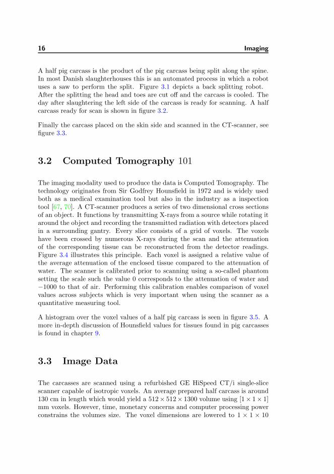
A half pig carcass is the product of the pig carcass being split along the spine.In most Danish slaughterhouses this is an automated process in which a robotuses a saw to perform the split. Figure 3.1 depicts a back splitting robot.After the splitting the head and toes are cut off and the carcass is cooled. Theday after slaughtering the left side of the carcass is ready for scanning. A halfcarcass ready for scan is shown in figure 3.2.

Finally the carcass placed on the skin side and scanned in the CT-scanner, seefigure 3.3.

3.2 Computed Tomography 101

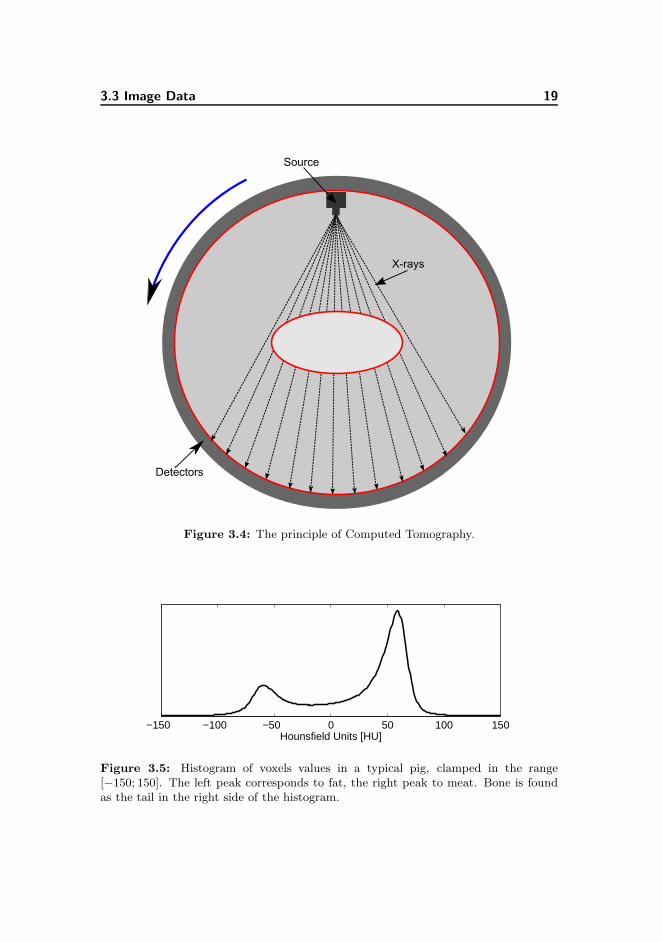
The imaging modality used to produce the data is Computed Tomography. Thetechnology originates from Sir Godfrey Hounsfield in 1972 and is widely usedboth as a medical examination tool but also in the industry as a inspectiontool [67, 70]. A CT-scanner produces a series of two dimensional cross sectionsof an object. It functions by transmitting X-rays from a source while rotating itaround the object and recording the transmitted radiation with detectors placedin a surrounding gantry. Every slice consists of a grid of voxels. The voxelshave been crossed by numerous X-rays during the scan and the attenuationof the corresponding tissue can be reconstructed from the detector readings.Figure 3.4 illustrates this principle. Each voxel is assigned a relative value ofthe average attenuation of the enclosed tissue compared to the attenuation ofwater. The scanner is calibrated prior to scanning using a so-called phantomsetting the scale such the value 0 corresponds to the attenuation of water and−1000 to that of air. Performing this calibration enables comparison of voxelvalues across subjects which is very important when using the scanner as aquantitative measuring tool.

A histogram over the voxel values of a half pig carcass is seen in figure 3.5. Amore in-depth discussion of Hounsfield values for tissues found in pig carcassesis found in chapter 9.

3.3 Image Data

The carcasses are scanned using a refurbished GE HiSpeed CT/i single-slicescanner capable of isotropic voxels. An average prepared half carcass is around130 cm in length which would yield a 512× 512× 1300 volume using [1× 1× 1]mm voxels. However, time, monetary concerns and computer processing powerconstrains the volumes size. The voxel dimensions are lowered to 1 × 1 × 10

3.3 Image Data 17

Figure 3.1: A back-splitting robot seen from the front. Courtesy of Danish MeatAssociation.

18 Imaging

Figure 3.2: A half carcass prepared and ready for scanning. Courtesy of DanishMeat Association.

Figure 3.3: A carcass wrapped in low density plastic about to be scanned. Courtesyof Danish Meat Association.

3.3 Image Data 19

Figure 3.4: The principle of Computed Tomography.

−150 −100 −50 0 50 100 150Hounsfield Units [HU]

Figure 3.5: Histogram of voxels values in a typical pig, clamped in the range[−150; 150]. The left peak corresponds to fat, the right peak to meat. Bone is foundas the tail in the right side of the histogram.

20 Imaging

Figure 3.6: An axial slice of the carcass volume located in the middle part.

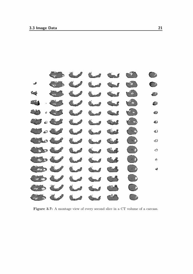
mm resulting in a reduction in the number of slices needed to cover the wholecarcass. This, however, results in a reduction in the resolution in the sagittaland coronal planes. Figure 3.6 shows a slice obtained in the middle part of thecarcass, while figure 3.7 depicts a montage of every second slice in the carcassvolume.

Other useful visualizations of the volume data borrows from medical imaging.Being a 3D volume two other views of a location in the carcass is needed to obtaincomplete visual coverage. Figure 3.8 depicts the midsagittal and midcoronalplanes of a carcass. Notice the jagged edges due to the reduced resolution. Othervisualizations tries to capture the 3D nature of the data. Figure 3.9 shows asimple method visualizing orthogonal slice planes. The volume effect is obtainedby arranging the axial, sagittal and coronal views in a three dimensional space.

3.3 Image Data 21

Figure 3.7: A montage view of every second slice in a CT volume of a carcass.

22 Imaging

Figure 3.8: Sagittal and coronal views of a carcass.

Figure 3.9: Volumetric visualization of a half carcass using orthogonal slice planes.

3.4 Anatomical Landmarks 23

Figure 3.10: X-Ray view of a carcass with landmarks overlain.

3.4 Anatomical Landmarks

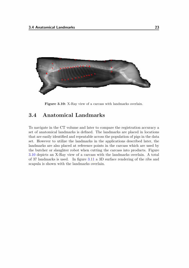
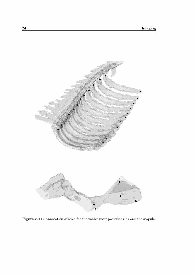
To navigate in the CT volume and later to compare the registration accuracy aset of anatomical landmarks is defined. The landmarks are placed in locationsthat are easily identified and repeatable across the population of pigs in the dataset. However to utilize the landmarks in the applications described later, thelandmarks are also placed at reference points in the carcass which are used bythe butcher or slaughter robot when cutting the carcass into products. Figure3.10 depicts an X-Ray view of a carcass with the landmarks overlain. A totalof 37 landmarks is used. In figure 3.11 a 3D surface rendering of the ribs andscapula is shown with the landmarks overlain.

24 Imaging

Figure 3.11: Annotation scheme for the twelve most posterior ribs and the scapula.

Part II

Algorithms for Image

Registration

Chapter 4

Introduction

The task of image registration can be phrased as the following [53]:

Given a so-called reference image R and a so-called template imageT , find a reasonable geometrical transformation such that a trans-formed version of the template image becomes similar to the refer-ence image.

This definition also lists the disciplines involved in image registration and inci-dently they are the topics of the chapters in this part of the thesis,

• Image transformation. Change to the geometry of the image.

• Similarity. Measure the goodness of the registration.

• Optimization. Control the transformations to maximize similarity.

• Regularization. Allow only reasonable transformations.

Each of the items listed is a research area in its own right, and as such thereexist a number of different algorithms and methods for each discipline.

In the course of this Ph.d. project a framework for 2D and 3D parametric imageregistration has been created. It is manifested in an implementation in Matlab

28 Introduction

capable of registration of large volumes. The following chapters are not by anymeans a comprehensive tutorial on image registration, but rather an overviewof the algorithms and concepts utilized in this framework.

4.1 Algorithms and Applications

4.1.1 Registration Algorithms

Image registration is a very active research area. Especially in the field ofmedical imaging but also in a variety of other applications. The applicationsand subsequent problems to solve in this thesis are very similar to problemsfound in medical imaging. Luckily this leaves a host of prior research in medicalimaging to lean upon. Consequently most literature found in this overviewstems from the medical imaging community.

Several methods and applications of image registration have been published.Books covering the topic of image registration are amongst others; Gothasby [49],Modersitzki [87] and Hajnal et al. [55]. Thorough surveys of the many algorithmsand applications can be found by Zitova and Flusser [137], by Pluim et al. [100],by Maintz and Viergever [86], by Lester and Arridge [81] and by Brown [18].Basically the task is to find the optimal dense field transforming a templateimage into a reference image. Several approaches exist.

A group of algorithms solves the problem using a variational approach. Twoparts are involved. One part models of the deformation of the underlying tissueregularizing the deformations. The other part is a measure quantifying thesimilarity of the images. These parts forms the basis of a system of non-linearpartial differential equations(PDE). In 1981 Broit [17] based his solution on thelinear theory of elasticity modeling the tissue as an elastic material and sinceother works [6, 15, 22, 40, 45, 87] has followed a similar approach.

Spearheaded by Christensen [22] was an approach where the image was regardedas a viscous fluid. The advantage over the elastic approach is that the fluid hasno ”memory” and as such can model larger deformations. Amongst others,algorithms have been made by Bro-Nielsen and Gramkow [16] and by Henn andWitsch [62].

Another approach using diffusion as a regularizer is proposed in Fischer andModersitzki [41]. An adaptation of this work is found in [42].

Solving the regularized problem without forming the PDE’s is found in theworks of Haber and Modersitzki [53, 54]. A similar method is found in the

4.1 Algorithms and Applications 29

algorithm by Hellier et al [60] however the similarity measure and regularizer isformulated using robust statistics. The Demons algorithm by Thirion [122] [123]is modeling the deformations via a diffusion process based on optical flow andGaussian smoothing of the deformation field. Recently the Demons algorithmhas been adapted and modernized in the work of Vercauteren et al. [126].

In the above mentioned algorithms no parameters are involved in the descriptionof the deformation field. However a host of algorithms parameterizing this fieldexist.

A very popular algorithm is based on Free Form Deformations and is described inRueckert et al [108, 111] and is based on the parametrization of the deformationfield using B-splines. A similar method also using B-splines is found in thethesis by Kybic [77]. In the works by Ashburner [4, 5] basis functions basedon the discrete cosine transform is used. Cootes et al. [32] ensures that thetransformation is diffeomorphic by constraining basis functions based on a cosinekernel.

Several software packages are available for image registration. Among them arethe popular AIR package [135], the tools NA-MIC [99], and the SPM package [5].

4.1.2 Applications

Image registration is used in a wide variety of applications. Most similar to theapplications found in this thesis are those based on atlases.

In the works of Cootes et al. [30, 32] and Twining et al. [127] image registrationis used to simultaneously build an atlas and automatically find the optimallandmark annotation. A groupwise cost function based on Minimum DescriptionLength [33] is used for simultaneous registration.

In a similar approach [117] Studholme uses a groupwise mutual information costfunction to simultaneously register a population of brains for spatial normaliza-tion.

In [12] Blezek et al. uses a technique named atlas stratification. Here they tryto infer from the image data whether one or multiple atlases is needed to bestdescribe the population.

In [94] Olafsdottir uses image registration to study craniofacial anomalies. Sta-tistical deformation models are built and statistics on the craniofacial abnor-malities of Crouzon Mice are inferred.

Atlases have many applications but the most similar to the application in this

30 Introduction

thesis is atlas based segmentation [10, 102, 104, 105]. Here the anatomical re-gions in the atlas is labeled. This labeling is then propagated onto the templatessegmenting one or several structures.

Chapter 5

Images and Image

Transformation

5.1 Images

By nature of the acquisition method digital images are discrete, but with thehelp of an interpolation scheme they can be viewed as being continuous. Inter-polation enables the evaluation of the image function anywhere in the domain.A wide variety of interpolation schemes exist [121].

Solving the problem of image registration is however done using discrete enti-ties. Thus a discretization of the continuous image is needed. This is done bysampling the image on a grid of points. For a D−dimensional image of sizen1 × . . .× nD voxels, the ith grid point is defined as,

xi = (x1i , . . . , x

Di )⊤. (5.1)

A grid is thus a collection of grid points and is here defined as a vector. A 3Dgrid of size n1 × n2 × n3 is a vector of size 3N × 1 with N = n1n2n3. In thiswork a grid has a certain lexicographical order. Grouping the ordinates x1

i , x2i

32 Images and Image Transformation

and x3i of all the grid points into three auxiliary vectors,

x1 =(

x11 . . . x

1N

)⊤(5.2)

x2 =(

x21 . . . x

2N

)⊤

x3 =(

x31 . . . x

3N

)⊤,

the 3D grid X is defined as,

X =[

x1⊤ x2⊤ x3⊤]⊤

. (5.3)

Sampling an image on a discrete grid is also a task for the interpolation scheme.A sample from a continuous image T at the grid point xi is written as,

T (xi) = T (xi) . (5.4)

A discrete image is denoted,

T (X) = T (X) (5.5)

where X indicates samples on an entire grid.

In the literature the dominating interpolation method is linear interpolation.The force of linear interpolation is its ease and resulting speed of computationrequiring only eight samples in 3D. However it is only C0 continuous and is assuch not differentiable. Another widely used scheme is based on cubic B-splinesand is C2 continuous, but significantly more computationally demanding. See[120] for a discussion of the merits of B-spline interpolation in image registration.

When working with images it is important to use physical coordinates. For-tunately data obtained from medical imaging devices, such as a CT-scannercontain information about the size of voxels, the orientation of the patient andso on. The relation between a 3D physical coordinate xi and a voxel coordinatexi is simply,

xi =

h1 0 00 h2 00 0 h3

x1i

x2i

x3i

, (5.6)

where the origo and orientation of the physical image is coincident with thevoxel image. h1,h2 and h3 are the physical dimensions of a voxel. Thus the gridcoordinates are given in metric units.

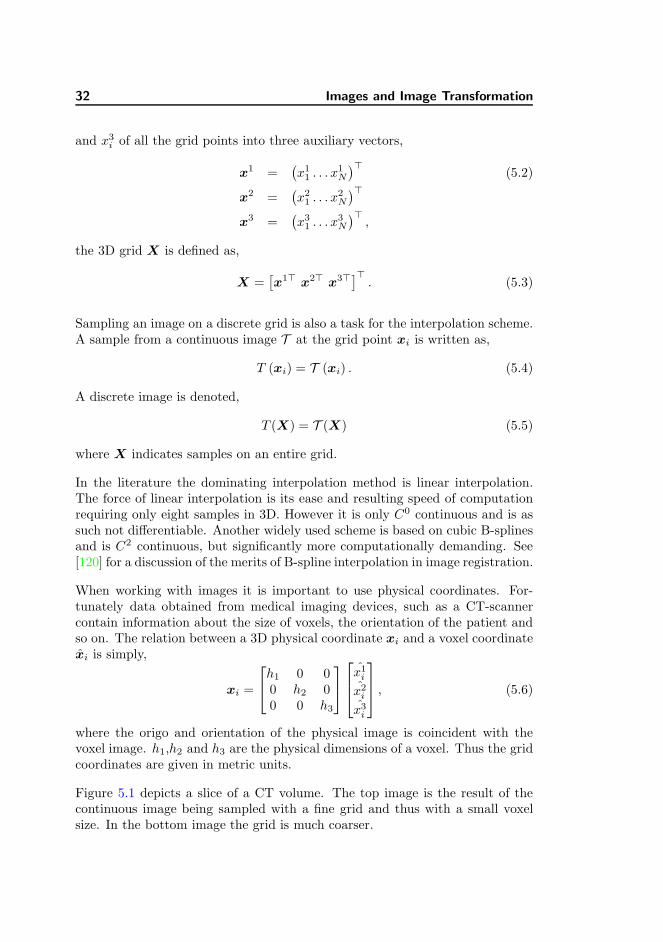
Figure 5.1 depicts a slice of a CT volume. The top image is the result of thecontinuous image being sampled with a fine grid and thus with a small voxelsize. In the bottom image the grid is much coarser.

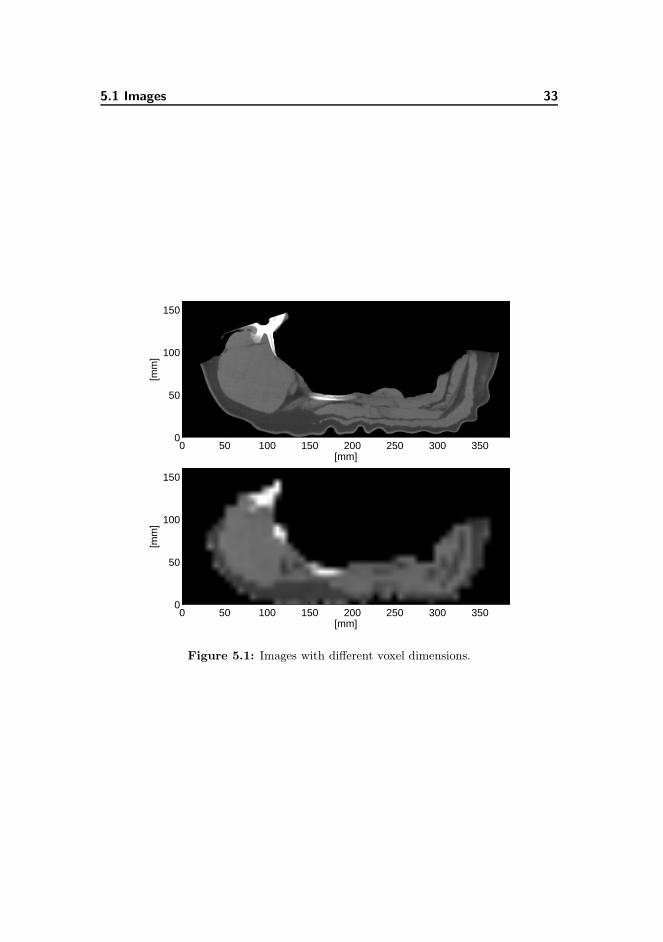
5.1 Images 33

[mm]

[mm

]

0 50 100 150 200 250 300 3500

50

100

150

[mm]

[mm

]

0 50 100 150 200 250 300 3500

50

100

150

Figure 5.1: Images with different voxel dimensions.

34 Images and Image Transformation

5.2 Image Transformations

In order to make two different images similar one or both has to change. This isthe task of image transformation. It involves transforming the underlying gridpoints by some function,

yi = φ (xi) , (5.7)

and the transformed image is then obtained by evaluating the continuous imageT with a transformed grid Y ,

T (Y ) = T (Y ), (5.8)

using an interpolation scheme.

The transformation can also be seen as a sum of an identity part and a defor-mation part,

y1i = x1i + u1(xi) (5.9)

y2i = x2i + u2(xi)

y3i = x3i + u3(xi),

where ud(xi) is the displacement of a grid point xi in the dth dimension. Thusfor each grid point there is a corresponding displacement vector,

ui =(

u1(xi) u2(xi) u

3(xi))⊤

. (5.10)

All the displacement vectors of the entire grid form a field. In the literature thisfield is known as the deformation field or the displacement field. Using the samelexicographical ordering rules as for a grid X indicated in equation 5.2 and 7.1the displacement vector can be stacked in a vector U . Thus the transformedgrid can also be written as,

Y = X +U . (5.11)

Figure 5.2 shows an example of an image transformation. The bottom left imageshows the image T (X) before transformation. The top left plot show the gridX with the displacement vectors overlain. The bottom right figure depicts thetransformed image T (Y ) produced by interpolating the left image using theresulting grid Y shown in the top right figure.

It is possible to parameterize the transformation in equation 5.9 using linear

5.2 Image Transformations 35

Figure 5.2: Example of an image transformation turning a square into a circle. Thetop left figure depicts the grid X overlaid with the displacement vectors. Top left isthe resulting grid Y . In the bottom row is shown the image before T (X) (left) andafter T (Y ) (right) the transformation.

36 Images and Image Transformation

combinations of basis functions. The expression then becomes,

y1i = x1i +

m∑

j

bj(xi)w1j (5.12)

y2i = x2i +

m∑

j

bj(xi)w2j

y3i = x3i +

m∑

j

bj(xi)w3j ,

where wdj is the weight of the jth basis function in the dth dimension. A vast

amount of possible basis function exist and are used in the literature [5, 29, 108].Encoding the basis function evaluations in a matrix Q with the element at theith row in the jth column being qij = bj(xi) enables simplification of the aboveexpression. Considering the entire grid X the transformation can be written as,

Y = X + I3 ⊗Qw, (5.13)

where I3 is a unit matrix of rank 3 and w is a vector of the parameters as in,

w =(

w1⊤ w2⊤ w3⊤)⊤

, (5.14)

and

w1 =(

w11 . . . w

1m

)⊤(5.15)

w2 =(

w21 . . . w

2m

)⊤

w3 =(

w31 . . . w

3m

)⊤

.

In general we want the deformation field to be smooth. If the application is sim-ply to make the images as similar as possible the regularity of the resulting gridis of no concern. Figure 5.3 depicts such a situation. A rectangle is transformedcompletely into a circle. However the resulting grid shows a large amount of foldover. In this case the grid is degenerate and the inverse transformation cannotbe recovered. Statistics on the deformations would be useless and registrationbased segmentation would not be possible. A measure often used in the liter-ature [53, 61] to determine if fold-over has occurred is the determinant of theJacobian of the displacement vectors.

5.3 Affine Transformations

In many image registration applications it is desirable to remove effects from theimage acquisition process. For instance in an experiment calculating statistics

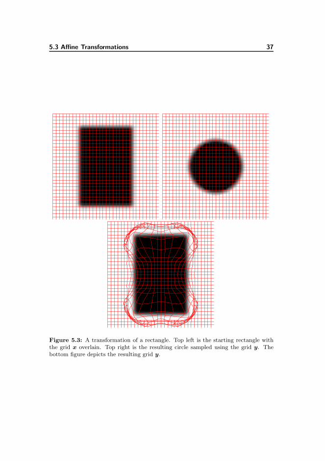
5.3 Affine Transformations 37

Figure 5.3: A transformation of a rectangle. Top left is the starting rectangle withthe grid x overlain. Top right is the resulting circle sampled using the grid y. Thebottom figure depicts the resulting grid y.

38 Images and Image Transformation

on the shape of objects effects such as how the object is placed in the scannershould not be a factor. To remedy this the images are preregistered usinglinear transformations. The most flexible linear transformation is the affinetransformation, which can model rotation, translation, scaling and shearing.For a 3D grid it is written as,

y1iy2iy3i

=

a1 a2 a3 a4a5 a6 a7 a8a9 a10 a11 a12

x1i

x2i

x3i

1

(5.16)

or expressed using basis functions,

y1i = xdi +

4∑

j=1

w1j qj (xi) (5.17)

y2i = xdi +

4∑

j=1

w2j qj (xi)

y3i = xdi +

4∑

j=1

w3j qj (xi) ,

where wdj is the jth coefficient for the corresponding basis function qj in the dth

dimension. The very simple basis functions are,

q1 (xi) = x1i , q2 (xi) = x2

i , q3 (xi) = x3i , q4 (xi) = 1. (5.18)

Considering the entire grid and putting in matrix notation this yields,

Y = X +

Q 0 0

0 Q 0

0 0 Q

w = X + I3 ⊗Qw, (5.19)

Y is the transformed grid, Q is a N×4 matrix of basis function evaluations andw is a 12 × 1 vector of coefficients. Figure 5.4 shows an example off an affinetransformation.

5.4 B-Spline Transformations

A type of transformation capable of modeling non-linear deformations is basedon B-splines. B-splines are widely used as a basis in image registration [77, 108].B-splines has very nice properties such as minimal support for a given order of

5.4 B-Spline Transformations 39

Figure 5.4: Affine transformation of a square. The left figure depicts the squareand the grid before transformation, while the middle figure shows the square with thetransformed grid. The right figure shows the square sampled using the transformedgrid.

approximation, and they are maximally continuous [121, 128]. Thus a cubic B-spline is C2 continuous and are non-zero only in four neighboring knot intervals.

Using a non-recursive definition [121] the following 1D cubic B-splines basisfunctions can be derived,

bj(xi) =

(2 + xi)3 for −2 ≤ xi < −1

−(3xi + 6)x2i + 4 for −1 ≤ xi < 0

(3xi − 6)x2i + 4 for 0 ≤ xi < 1

(2− xi)3 for 1 ≤ xi < 2

0 otherwise

(5.20)

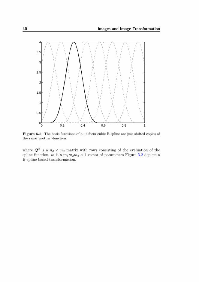
The basis for a cubic B-spline with equidistantly placed knots is simply shiftedcopies of the ’mother’ function in equation 5.20. Figure 5.5 depicts the basisfunctions of a cubic B-spline using free boundary conditions.

B-splines are separable and so it is easy to extend the basis functions to 3D.The transformation is written as

y1i = x1i +

m1∑

j=1

m2∑

k=1

m3∑

l=1

bj(x1i )bk(x

2i )bl(x

3i )w

1jkl (5.21)

y2i = x2i +

m1∑

j=1

m2∑

k=1

m3∑

l=1

bj(x1i )bk(x

2i )bl(x

3i )w

2jkl

y3i = x3i +

m1∑

j=1

m2∑

k=1

m3∑

l=1

bj(x1i )bk(x

2i )bl(x

3i )w

3jkl,

where m1,m2 and m3 are the number of equidistantly placed knots for thesplines. In matrix notation using the tensor product property,

Y = X + I3 ⊗Qw = X + I3 ⊗Q3 ⊗Q2 ⊗Q1w, (5.22)

40 Images and Image Transformation

0 0.2 0.4 0.6 0.8 10

0.5

1

1.5

2

2.5

3

3.5

4

Figure 5.5: The basis functions of a uniform cubic B-spline are just shifted copies ofthe same ’mother’-function.

where Qd is a nd × md matrix with rows consisting of the evaluation of thespline function, w is a m1m2m3 × 1 vector of parameters Figure 5.2 depicts aB-spline based transformation.

Chapter 6

Image Registration - a Large

Scale Optimization Problem

6.1 Similarity Measurements

Succeeding in making images similar requires a quantitative measure of thegoodness of the registration. It also involves an algorithm to control the imagetransformations such that similarity is maximized. In this thesis an optimiza-tion approach is chosen. Using parametric transformations it naturally becomesan optimization of the similarity with regards to the parameters. Using opti-mization community lingo the similarity measure is often called a cost functionor an objective function.

Similarity is usually determined by comparing values of corresponding voxels. Ahost of different similarity measures exist. One of the most dominant, especiallyin the medical imaging community, is Mutual Information [44, 85, 133] whichis suited for comparison of multi-modality images [118] or when contrast agentsare applied. Another often used measure is based on the normalized cross-correlation coefficient [26, 80].

In this thesis the focus is on images acquired using a CT-scanner. The scanneris calibrated with a phantom as part of the preparation. This means that X-rayattenuation of corresponding tissue types are directly comparable across scans.

42 Image Registration - a Large Scale Optimization Problem

A similarity measure suited for this situation is the sum-of-squared-differences(SSD) measure. It assumes that the differences in value of corresponding vox-els are independently, identically normally distributed. SSD measures the Eu-clidean distance between grey values of corresponding voxels in a reference imageR and a template image T ,

D(Y ) =h

2

∑

i

(T (yi)−R(xi))2

(6.1)

=h

2‖T (Y )−R(X)‖2L2,

with h = h1h2h3 being the product of the voxel dimensions. Maximizing imagesimilarity thus requires a minimization of SSD. Since the minimization is drivenby parametric image transformations, equation 6.1 is phrased as a function ofw,

D(w) =h

2‖T (w)−R‖2, (6.2)

where the subscript L2 indicating the Euclidean norm is left out and R = R(X).A key benefit of minimizing SSD is that it is a least-squares problem. Solvingleast-square problems is part of a vast amount of data fitting and modelingapplications and several tried and tested algorithms exist [93].

6.1.1 Non-Linear Least-Squares

When minimizing equation 6.2 it would be preferable to find the value of wfor which the measure has the lowest value possible. In other words to finda global minimizer. In most image registration problems this is however notfeasible. Thus, we have to settle for a local minimizer, defined by Nocedal andWright [93] as the value w∗ for which D(w∗) ≤ D(w) for w belonging to someneighborhood of w∗. In other words w∗ is at the bottom of a valley in the costfunction landscape. To determine that a point w∗ is a minimizer of equation6.2 we need information of the function in the neighborhood. A way to obtainthis information is by Taylor expanding D,

D(w + s) = D(w) + s⊤∇D(w) +1

2s⊤∇2D(w)s+O(‖s‖)3, (6.3)

where ∇D is the gradient and ∇2D is the Hessian matrix.

Finding the minimizer is often done by an iterative algorithm. From a startingpoint the parameters w are updated with a vector sk pointing in the directionof lower values of the function D,

wk+1 = wk + sk, (6.4)

6.2 The Gauss-Newton Method 43

and stops when certain criteria are met. To determine the update sk two dom-inating schemes exist, namely line search and trust region methods. The algo-rithms in this thesis use the line search strategy and so it is described below.Trust region methods are by no means inferior but for the sake of compactnessthey are left out. An extensive introduction can be found in [93].

The benefit of SSD being a least-squares problem comes in the composition ofthe gradient and Hessian. For ease of presentation equation 6.2 can also bephrased in terms of the vector of residuals r = T (w)−R,

D(w) =h

2(T (w)−R)⊤(T (w)−R) =

h

2r⊤r. (6.5)

Thus the gradient is,

∇D(w) = h∇r⊤r = hJ(w)⊤r, (6.6)

where J(w) is the Jacobian which is the matrix of first partial derivatives of theresiduals,

J(w) =

∂r1∂w1

· · · ∂r1∂wm

.... . .

∂rn∂w1

· · · ∂rn∂wm

. (6.7)

The corresponding Hessian is,

∇2D(w) = h∇r⊤∇r + h∇2rr = hJ(w)⊤J(w) + h∇2rr. (6.8)

Because the first part is by far the most dominating most algorithms skip theevaluation of the second derivatives. Furthermore, in image registration prob-lems it is generally not recommended to evaluate the second derivatives of im-ages [87]. When the Jacobian is evaluated it can be seen that the first part ofthe Hessian J(w)⊤J(w) comes for ”free”.

6.2 The Gauss-Newton Method

A local minimizer has the lowest local value of D(w) and so the line searchstrategy is simply a matter of going downhill in the cost function landscape.Two problems exists. The first is finding a descent direction sk, and the secondis to determine the size α of the step to take.

An obvious path would be to go in the direction of fastest decay of the costfunction or more accurately in the direction of steepest descent as in −∇D.

44 Image Registration - a Large Scale Optimization Problem

However as stated in any textbook on optimization this will be extremely slowon all but the simplest problems. In general a descent direction is defined as,

s⊤k∇D(wk) < 0. (6.9)

i.e. a direction with an angle in the open interval ] − π/2, pi/2[ to −∇D. Amuch better choice would be to include information from the Hessian and so weend up with the Newton direction,

sk = −∇2D(wk)−1∇D(wk), (6.10)

assuming that the second derivative exists and is positive definite.

Utilizing the benefits of least-squares problems equation 6.10 leads to a verysimple iterative algorithm namely the Gauss-Newton method. It revolves aroundsolving the linear system also known as the normal equations [93],

J⊤

k Jksk = −J⊤

k (T (w)−R) , (6.11)

where Jk is the Jacobian J(wk).

As seen the Gauss-Newton algorithm only involves calculating the residuals andthe Jacobian. For parametric image registration the Jacobian is,

J(w) =∂ (T (Y )−R)

∂w, (6.12)

which by using the chain-rule is found to be,

Jk = ∇TQ =[

∇T 1∇T 2

∇T 3]

I3 ⊗Q3 ⊗Q2 ⊗Q1, (6.13)

where each∇T d is a diagonal matrix containing the partial derivatives ∂T (yi)/∂xd

of the image T .

The listing in algorithm 6.1 sketches the Gauss-Newton algorithm for imageregistration. To stop the algorithm certain criteria can be set. These criteriashould prevent the algorithm from running when no progress is made. Oftenused are; the decrease in cost function D(wk−1)−D(wk) < ǫD, the size of theJacobian ‖Jk‖ < ǫJ , the difference in parameters ‖sk−1 − sk‖ < ǫs or of coursethe number of iterations k > kmax.

6.3 Step Length

For a minimizer w∗ two conditions exist. A first order condition on the gradient,

∇D(w∗) = 0, (6.14)

6.3 Step Length 45

Algorithm 6.1 Gauss-Newton algorithm

1: Set starting guess w = w0

2: while NOT STOP do

3: Transform the grid Y = X +Qw.4: Compute T (Y ) and ∇T (Y ).5: Get sk by solving the linear system in equation 6.11.6: Calculate step length α using algorithm 6.2 or 6.3.7: Update wk+1 = wk + α∆wk

8: end while

requiring the minimizer to be at a stationary point. A second order conditionon the Hessian ∇2D,

∇2D(w∗) must be positive semidefinite, (6.15)

requiring the function to be convex at the position of the minimizer.

Choosing the right step length parameter α is an important task and has impacton the convergence rate of the optimization algorithm. It is basically a onedimensional problem, namely minimizing,

φ(α) = D(w + αsk) (6.16)

with respect to α. However solving the problem exactly can be computationallyvery costly and unnecessary if we relax on the quality of the minimization. Twoconditions known as the Wolfe conditions exist and it can be shown that stepssatisfying these yield acceptable convergence rates [93].

The first Wolfe condition guarantees sufficient decrease in the cost function,

φ(α) ≤ φ(0) + c1φ′(0)α (6.17)

where c1 ∈ (0, 1). This ensures a decrease of the cost function at least a factorc1 more than the one predicted by the slope of the cost function at the startingpoint. A simple method is listed in algorithm 6.2 in which α meets the criteriaset by equation 6.17. It backtracks from a starting value until a stopping criteriais enforces. Of course the initial value for α, τ , c1 and the number of line searchiterations can be set by the user. The backtracking algorithm also makes surethat the step taken is not too short. It backtracks from steps that are too longuntil an acceptable α is found. The optimal value of α is within an the interval(αl/τ, αl) where αl is the last value rejected.

The second Wolfe condition is important in algorithms where steps of lengthslarger than 1 are required. The second Wolfe condition is stated below,

|φ′(α)| ≤ c2|φ′(0)|, (6.18)

46 Image Registration - a Large Scale Optimization Problem

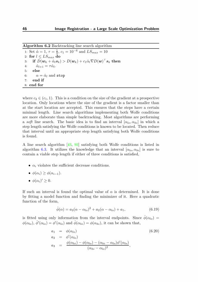
Algorithm 6.2 Backtracking line search algorithm

1: Set α = 1, τ = 12 , c1 = 10−6 and LSmax = 10

2: for l ≤ LSmax do

3: if D(wk + αlsk) > D(wk) + c1αl∇D(w)⊤sk then

4: αl+1 = ταl.5: else

6: α = αl and stop

7: end if

8: end for

where c2 ∈ (c1, 1). This is a condition on the size of the gradient at a prospectivelocation. Only locations where the size of the gradient is a factor smaller thanat the start location are accepted. This ensures that the steps have a certainminimal length. Line search algorithms implementing both Wolfe conditionsare more elaborate than simple backtracking. Most algorithms are performinga soft line search. The basic idea is to find an interval [αlo, αhi] in which astep length satisfying the Wolfe conditions is known to be located. Then reducethat interval until an appropriate step length satisfying both Wolfe conditionsis found.

A line search algorithm [43, 93] satisfying both Wolfe conditions is listed inalgorithm 6.3. It utilizes the knowledge that an interval [αlo, αhi] is sure tocontain a viable step length if either of three conditions is satisfied,

• αi violates the sufficient decrease conditions.

• φ(αi) ≥ φ(αi−1).

• φ(αi)′ ≥ 0.

If such an interval is found the optimal value of α is determined. It is doneby fitting a model function and finding the minimizer of it. Here a quadraticfunction of the form,

φ(α) = a3(α− αlo)2 + a2(α− αlo) + a1, (6.19)

is fitted using only information from the interval endpoints. Since φ(αlo) =

φ(αlo), φ′(αlo) = φ′(αlo) and φ(αhi) = φ(αhi), it can be shown that,

a1 = φ(αlo) (6.20)

a2 = φ′(αlo)

a3 =φ(αhi)− φ(αlo)− (αhi − αlo)φ

′(αlo)

(αhi − αlo)2,

6.4 Solving the Linear Problem 47

and thus the minimizer is,

α = αlo −φ′(αlo)

2a3. (6.21)

If the quadratic is concave the midpoint between αlo and αhi is chosen. No-tice however if the starting value of α is acceptable the algorithm terminateimmediately.

Algorithm 6.3 Line search algorithm satisfying both Wolfe conditions

1: Set k = 0, α0 = 0, τ = 2, c1 = 10−6, c2 = 0.9 and LSmax = 102: while k < LSmax do

3: if φ(α)k > φ(0) + c1φ′(0)α then

4: α = reduce(αk−1, αk) and stop

5: end if

6: if |φ′(α)k| ≤ −c2φ′(0) then

7: α = αk and stop

8: end if

9: if φ′(α)k ≥ 0 then

10: α = reduce(αk, αk−1) and stop

11: end if

12: αk+1 = ταk

13: k = k + 114: end while

6.4 Solving the Linear Problem

As seen above all algorithm for least-square optimization revolves around solvinga linear system of equation. An extensive number of algorithms for solvingthis problem directly exist. However solving 3D or even 2D image registrationproblems the size of the matrices and vectors involved prohibits the use of directsolvers. For instance a registration problem involving a 512× 512× 140 imagewith 200× 200× 100 basis functions, the image will contain 36, 700, 160 voxels,the matrix Q will have the size 110, 100, 480 × 12, 000, 000 and the vector w

will have 12, 000, 000 elements. Even the sparsity of Q will not make solvingthis problem directly possible. The sections below presents tricks to make thesolution attainable using properties of the basis functions and iterative schemesfor solving the linear systems.

48 Image Registration - a Large Scale Optimization Problem

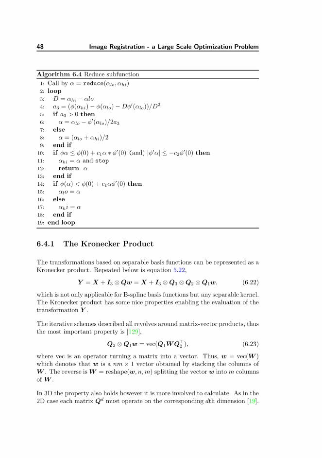
Algorithm 6.4 Reduce subfunction

1: Call by α = reduce(αlo, αhi)2: loop

3: D = αhi − αlo4: a3 = (φ(αhi)− φ(αlo)−Dφ′(αlo))/D

2

5: if a3 > 0 then

6: α = αlo − φ′(αlo)/2a37: else

8: α = (αlo + αhi)/29: end if

10: if φα ≤ φ(0) + c1α ∗ φ′(0) (and) |φ′α| ≤ −c2φ

′(0) then11: αhi = α and stop

12: return α13: end if

14: if φ(α) < φ(0) + c1αφ′(0) then

15: αlo = α16: else

17: αhi = α18: end if

19: end loop

6.4.1 The Kronecker Product

The transformations based on separable basis functions can be represented as aKronecker product. Repeated below is equation 5.22,

Y = X + I3 ⊗Qw = X + I3 ⊗Q3 ⊗Q2 ⊗Q1w, (6.22)

which is not only applicable for B-spline basis functions but any separable kernel.The Kronecker product has some nice properties enabling the evaluation of thetransformation Y .

The iterative schemes described all revolves around matrix-vector products, thusthe most important property is [129],

Q2 ⊗Q1w = vec(Q1WQ⊤

2 ), (6.23)

where vec is an operator turning a matrix into a vector. Thus, w = vec(W )which denotes that w is a nm × 1 vector obtained by stacking the columns ofW . The reverse is W = reshape(w, n,m) splitting the vectorw into m columnsof W .

In 3D the property also holds however it is more involved to calculate. As in the2D case each matrix Qd must operate on the corresponding dth dimension [19].

6.4 Solving the Linear Problem 49

A method for calculating the product is depicted in algorithm 6.5. The algo-rithm operates with a 3D dimensional tensor W which is made by reshapinga vector Wi,j,k = wi+m1j+m2k. Furthermore two operations has to be defined.First an operation analogous to matrix transpose, a cyclic rearrangement so thelast dimension becomes the first, i.e. R

m1×m2×m3 → Rm3×m1×m2 . Secondly

a multiply operation similar to matrix-matrix multiplication but operating oneach submatrix along the third dimension of the tensor. This enables the mul-

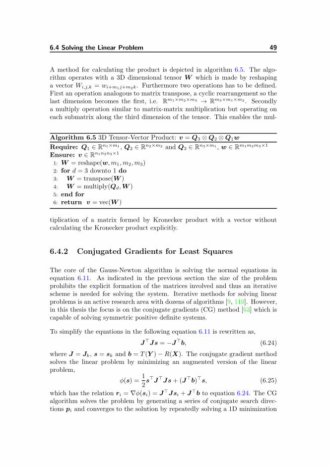
Algorithm 6.5 3D Tensor-Vector Product: v = Q3 ⊗Q2 ⊗Q1w

Require: Q1 ∈ Rn1×m1 , Q2 ∈ R

n2×m2 and Q3 ∈ Rn3×m1 , w ∈ R

m1m2m3×1

Ensure: v ∈ Rn1n2n3×1

1: W = reshape(w,m1,m2,m3)2: for d = 3 downto 1 do

3: W = transpose(W )4: W = multiply(Qd,W )5: end for

6: return v = vec(W )

tiplication of a matrix formed by Kronecker product with a vector withoutcalculating the Kronecker product explicitly.

6.4.2 Conjugated Gradients for Least Squares

The core of the Gauss-Newton algorithm is solving the normal equations inequation 6.11. As indicated in the previous section the size of the problemprohibits the explicit formation of the matrices involved and thus an iterativescheme is needed for solving the system. Iterative methods for solving linearproblems is an active research area with dozens of algorithms [9, 110]. However,in this thesis the focus is on the conjugate gradients (CG) method [63] which iscapable of solving symmetric positive definite systems.

To simplify the equations in the following equation 6.11 is rewritten as,

J⊤Js = −J⊤b, (6.24)

where J = Jk, s = sk and b = T (Y )−R(X). The conjugate gradient methodsolves the linear problem by minimizing an augmented version of the linearproblem,

φ(s) =1

2s⊤J⊤Js + (J⊤b)⊤s, (6.25)

which has the relation ri = ∇φ(si) = J⊤Jsi + J⊤b to equation 6.24. The CGalgorithm solves the problem by generating a series of conjugate search direc-tions pi and converges to the solution by repeatedly solving a 1D minimization

50 Image Registration - a Large Scale Optimization Problem

problem along each search direction to gain the next iterate. The solution ofthe quadratic in equation 10.3 along the direction pi is given by,

αi = −r⊤

i pi

p⊤

i J⊤Jpi

, (6.26)

yielding updates similar to a line search method,

si+1 = si + αipi. (6.27)

Multiplying equation 6.27 with J⊤J and adding J⊤b on both sides yields,

ri+1 = ri + αiJ⊤Jpi. (6.28)

The next conjugate search directions pi+1 is generated using only the previousdirection pi,

pi+1 = −ri + βipi, (6.29)

where the scaler βk can be shown to be [93],

βi =r⊤

i+1J⊤Jpi

p⊤i J

⊤Jpi

. (6.30)

Equation 6.29 and the following properties of conjugate directions,

r⊤

i pj = 0 for j = 0, 1, . . . , i− 1 (6.31)

r⊤

i rj = 0 for j = 0, 1, . . . , i− 1,

simplifies equations 6.26 and 6.30 to,

αi =r⊤

i ri

p⊤i J

⊤Jpi

, (6.32)

βi =r⊤

i+1ri+1

r⊤

i ri(6.33)

The condition number of the matrix J⊤J is the square of the condition numberof J and this has an impact on the convergence rate of CG [9]. Fortunately theproducts involving J⊤J can be split in two parts. First the residuals can bephrased as,

ri = J⊤(Jxi + b) = J⊤zi, (6.34)

which leads to the residual update,

zi+1 = zi + αiJpi (6.35)

ri+1 = J⊤zi+1.

6.5 Regularization 51

Introducing a auxiliary vector qi = Jpi equation 6.32 simplifies to

αi =r⊤i ri

q⊤

i qi(6.36)

Now we have assembled the building block of the conjugated gradients algo-rithm. A listing can be found in algorithm 6.6.

Algorithm 6.6 CG for Least-squares: J⊤Jx = J⊤b

1: while NOT STOP do

2: Set x0 = 0, z0 = Jx0 − b , r0 = J⊤z0, p0 = −z03: qi = Jpi

4: αi =r⊤

i ri

q⊤

iqi

5: xi+1 = xi + αipi

6: zi+1 = zi + αiqi7: ri+1 = J⊤zi+1

8: βi =r⊤

i+1ri+1

r⊤

iri

9: pi+1 = −ri + βipi

10: end while

6.5 Regularization

Image registration by simply minimizing equation 6.2 is not usable in practise.There is two reasons for this. One is that the problem is very ill-posed inthat the solution is very dependent on the noise in the image data [87]. Thesecond reason is there is nothing in the optimization that ensures the optimaltransformation is reasonable [53], e.g. if the deformation field is folded. Theremedy of this is to use regularizing which act both as a smoother reducingthe ill-posedness of the problem but also ensuring the right properties of theresulting transformation.

6.5.1 Implicit Regularization

Image registration based on transformations parameterized using basis functionscontains an implicit regularization. The transformations allowed are restrictedto the space spanned by the parameters. An example is the affine transformationdiscussed earlier where only shearing, rotation and translation are allowed.

52 Image Registration - a Large Scale Optimization Problem

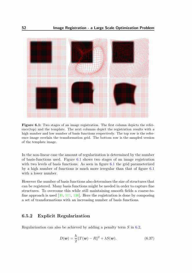
Figure 6.1: Two stages of an image registration. The first column depicts the refer-ence(top) and the template. The next columns depict the registration results with ahigh number and low number of basis functions respectively. The top row is the refer-ence image overlain the transformation grid. The bottom row is the sampled versionof the template image.

In the non-linear case the amount of regularization is determined by the numberof basis-functions used. Figure 6.1 shows two stages of an image registrationwith two levels of basis functions. As seen in figure 6.1 the grid parameterizedby a high number of functions is much more irregular than that of figure 6.1with a lower number.

However the number of basis functions also determines the size of structures thatcan be registered. Many basis functions might be needed in order to capture finestructures. To overcome this while still maintaining smooth fields a coarse-to-fine approach is used [30, 111, 136]. Here the registration is done by composinga set of transformations with an increasing number of basis functions.

6.5.2 Explicit Regularization

Regularization can also be achieved by adding a penalty term S in 6.2,

D(w) =h

2‖T (w)−R‖2 + λS(w). (6.37)

6.5 Regularization 53

The exact form of the regularizing term depends on the application. One of themost widely used regularizers is Tikhonov Regularization [125]. The formulationof the cost function in equation 6.37 is then,

D(w) =h

2‖T (w)−R‖2 + λ‖Bw‖2. (6.38)

Typical choices of the matrix B are the first or second derivative operator,

Other types of regularizers tries to induce physical properties into the smooth-ness requirements of the resulting displacement field. A group of such regular-izers are elastic [17], fluid [15, 16, 22, 45], diffusion [41, 53] and many more [87].Others regularize on the bending energy [13], or add volume preserving con-straints [54, 103].

In this work a regularizer based on the diffusion equation is used and thus theregularizing term is [87],

S(U) = ‖∇U‖2, (6.39)

and since U = Qw this can be phrased as in equation 6.38 in terms on theparameters,

S(w) = ‖∇Qw‖2, (6.40)

where ∇Q is plays the part of the regularizing matrix B from equation 6.38.

The value of the regularization parameter λ can be estimated by plotting anL-curve[58], using generalized cross-validation or by visual inspection [53].

6.5.3 Solving the Augmented Problem

As seen from equation 6.37 the regularizer is an added term to the cost function.

(

J⊤

k Jk + λB⊤B)

sk = −(

Jk + λB⊤B)⊤

(T (Y )−R (X)) , (6.41)

where the augmented Jacobian is,

Jλk = Jk + λB⊤B. (6.42)

In the case of the diffusion regularizer from equation 6.40, the matrix ∇Q isdefined as [5, 87],

∇Q =(

∇Q⊤

3 ∇Q3

)

⊗(

Q⊤

2 Q2

)

⊗(

Q⊤

1 Q1

)

(6.43)

+(

Q⊤

3 Q3

)

⊗(

∇Q⊤

2 ∇Q2

)

⊗(

Q⊤

1 Q1

)

+(

Q⊤

3 Q3

)

⊗(

Q⊤

2 Q2

)

⊗(

∇Q⊤

1 ∇Q1

)

,

54 Image Registration - a Large Scale Optimization Problem

Figure 6.2: Reference and resulting grid y and resulting T (y)using a diffusion regu-larizer for the same problem as in figure 6.1.

where ∇Qd indicates the matrix of first derivatives of the basis functions in thedth dimension. This augmented problem is also quite large but using Kroneckerproducts makes the use of algorithm 6.6 applicable. Figure 6.2 depicts a reg-istration of the same squares as in figure 6.1 but using a diffusion regularizer.

6.6 Parametric Image Registration Algorithm

As explained above image registration involves similarity measure, interpolation,image transformation, optimization, and regularization. Now all the pieces ofan image registration algorithm are present.

As any optimization problem registration is prone to converge to a local minima.To overcome this a multi-resolution, or pyramid, approach is used [1, 107].Figure 6.3 depicts an image pyramid obtained by successively downsampling theoriginal image. This is a widely used method in image processing and is adoptedin many image registration algorithms found in the literature [32, 53, 111, 136].Basically it is a coarse to fine approach, using a series of downsampled versions ofthe reference and template. Registration is done on the coarse level propagatingthe result onto the level above. This has several benefits such as regularization,reduces the number of local minima, provides a good starting guess for theoptimization on the next level and reduces computing time.

The algorithm for non-linear registration presented in this thesis consist oftwo steps; a preregistration step using affine transformations and a non-linearstep using the B-spline basis function method. Both uses the multi-resolutionmethod. Listing 6.7 sketches an algorithm for multi-resolution image registra-tion. The propagation step in line 5 of algorithm 6.7 differs between the affinestep and the non-linear step. Due to the use of physical coordinates the param-

6.6 Parametric Image Registration Algorithm 55

Figure 6.3: The image pyramid is made by downsampling the image number of times.The image can form a pyramid, hence the name.

Algorithm 6.7 Multilevel registration algorithm

1: Initialize w0,2: for l = lmin to lmax do

3: Rl ← R and Tl ← T transfer images to level l4: wl ← solve equation 6.2 or equation 6.37 using algorithm 6.15: wl+1 ← wl propagate parameters to next level6: end for

56 Image Registration - a Large Scale Optimization Problem

eters in the affine algorithm map directly to the next level, thus wk+1 = wk.However in the non-linear algorithm this is not the case.

The non-linear algorithm utilizes an hierarchical approach [79, 111, 136], similarto the multi-resolution method. Here the algorithm starts out using a coarseset of B-spline basic functions on the first level, and refines when a new level isreached and so on. For example an initial configuration of 10 × 10 × 10 basisfunctions might be refined to a 20 × 20 × 20, ending up with 100 × 100 × 100on the finest level. Thus there is no direct mapping of parameters from level tolevel. However an approximate solution can be found. The starting deformationgrid Ul+1 = Ql+1wl+1 on a finer level should be more or less equal to theresulting grid Ul = Qlw on a lower level. However the lower level grid must beprolongated so it has similar size as the fine level. This is done by resamplingthe basis functions corresponding to Ql and obtaining Q⋆

l . Thus the new set ofparameters wl+1 can be found by minimizing ‖Q⋆

lwl −Ql+1wl+1‖2 which has

the least squares solution

wl+1 =(

Q⊤

l+1Ql+1

)−1Ql+1Q

⋆l+1wl (6.44)

An algorithm is listed in algorithm 6.8 mapping the parameters by using theleast squares approach.

Algorithm 6.8 Propagation of basis-function parameters

1: obtain a finer grid Xl+1

2: obtain the coarser Q⋆l using Xl+1

3: obtain the finer Ql+1 using Xl+1

4: wl+1 ←(

Q⊤

l+1Ql+1

)−1Ql+1Q

⋆l+1wl

6.7 Evaluation of Image Registration

The usefulness of an image registration between two subject is not given bythe final value of the similarity metric. A number of other factors should bequantified in order to evaluate the performance [52, 86]. However validation ofan image registration is difficult since the ground truth rarely is available. Oftenthe validation is done by measuring the Euclidean distance between anatomicallandmarks placed by experts. Recently a project named ”Non-Rigid ImageRegistration Evaluation Project (NIREP)” [23] has been launched. The goal ofthe project is to develop a standard set of metrics to asses the performance ofregistration algorithms.

6.7 Evaluation of Image Registration 57

The performance of an registration algorithm must also reflect the application.In the case of mapping landmarks from a reference onto a template the Eu-clidean distance of landmark is applicable. Basically, the metric is a sum overL Euclidean distances,

Dlm =1

L

L∑

i=1

‖φ(xri)− xti‖ =1

L

L∑

i=1

‖xri + u(xri)− xti‖, (6.45)

where in u(xr) is the displacement in xr and is found by linearly interpolatingthe resulting displacement field U . See section 5.2. Another measure suited forregistration applications involving atlases is the Intensity Variance Metric [23].The underlying idea is that when a series of images is registered to the samereference the average of the transformed images should be sharp. Sharpnesscan be measured by computing the variance of the transformed images. Thevariance image is computed as,

Iiv =1

L

L∑

1

(Ti(yi)−A(x))2, (6.46)

where L is the number of transformed images and A = 1L

∑Li=1 Ti(yi) is the

average image.

58 Image Registration - a Large Scale Optimization Problem

Part III

Applications

Chapter 7

Virtual Jointing of Pig

Carcasses using Image

Registration

Martin Vester-Christensen and Lars Bager Christensen and Marchen Hviid andEli V. Olsen and Rasmus Larsen

Abstract

In the Danish pig slaughtering industry optimizing the use of each pig isof major importance. A large number of different cuts of each carcassis possible. Not all cuts are suited for each carcass due to their obviousanatomical difference. Optimal use is achieved by sorting the carcassesinto groups. During the slaughtering process a set of measurements of leanmeat percentage and weight is made on each carcass. These measurementsform the parameters used in the sorting. Thus lowering the anatomicalvariation within each group substantially. It is important to know the rela-tion between the quality of a cut, in this case the yield, and the measuredparameters in order to optimize the use of the carcasses. This calibrationis done by manually cutting carcasses and estimating quality of the indi-vidual cuts. This is very labor intensive and as such only a limited numberof carcasses is used.

In this paper a method for predicting the yield of two different productsis proposed. The anatomical relation of each carcass and a reference is

62 Virtual Jointing of Pig Carcasses using Image Registration

established using image registration of Computed Tomography(CT) scansof the carcasses. Using this relation a series of virtual cuts defined byanatomical landmarks can be propagated onto each carcass. The yields ofthese virtual cuts are calculated and related to the lean meat percentageand the carcass weight.

7.1 Introduction

The pig industry is one of the largest and most important industries in theDanish economy with an export value of approximately 28 billion DKK [113]. Asa consequence of increasing competition from slaughterhouses in countries withlower wages, optimization of all aspects of the slaughtering process is needed.The inhomogeneous nature of the pigs with obvious differences in weight, size,etc. makes optimal use difficult. The slaughterhouses tries to remedy this bysorting the carcasses into groups of similar properties. All carcasses in a groupis then cut into the same product. The sorting criteria and the sorting accuracyhas substantial influence on the economy of the slaughterhouses [75].

The carcasses can be used in a variety of different end-products. However yield,costs and prices determine the suitability of a carcass being cut as a particu-lar product. Yield of a product is defined as the fraction of meat versus thecombined weight of meat and fat in the product.

In order to ensure optimal use of the carcasses, it is important to have knowledgeof how well the carcasses fits a given cut. The slaughterhouses uses mathematicalmodels to predict the quality of particular cuts. These models are calibrated bymanually cutting a set of pigs into a given product. The quality, e.g. yield, ofthe cuts is then measured. This process is very labor intensive which constrainsthe number of carcasses used in the calibration. Furthermore a carcass can onlybe cut once, and thus its compatibility with other cuts cannot be established.

Recently research in the use of Computed Tomography(CT) as a tool in theDanish slaughterhouses has been undertaken. This paper is a preliminary studyin the use of CT as a tool for predicting the quality of specific uses of a pigcarcass in the Danish slaughterhouses.

Image registration is used to obtain an anatomical mapping between a referencecarcass and a set of template carcasses. To the reference is coupled a set ofanatomical landmarks. The use of these landmarks is two-fold; firstly theyare used a measure of registration accuracy and secondly a set of virtual cuts isdefined relatively to the landmarks. The anatomical mapping obtained from theimage registration is used to propagate the virtual cuts onto the set of carcasses.This enables the evaluation of the virtual cuts in all carcasses without the use

7.1 Introduction 63

of elaborate feature extraction schemes.

Two cuts of the middle part of the carcass are evaluated. A loin product whichis produced by cutting very close to the muscle longissimus dorsi. Furthermorean 18cm back product which is produced by making a cut parallel with the rindat a distance of 18cm from the rind edge. Simple models for the prediction ofthe yield in the loin and the 18cm back product are created. The parametersof the models are the total weight and the lean meat percentage. Two param-eters actually used in the slaughterhouses today. The method is evaluated bypredicting the yield of 57 carcasses.

7.1.1 Previous work

Earlier work using image analysis to virtually cut pig carcasses is found in [56].Hansen uses a slice by slice approach to virtually cut the 18cm back with goodresults. Features are extracted by searching radially from a predefined locationin the slice.

In this work the cuts are made on a 3D carcass volume using image registrationand the propagation of landmarks as the cutting algorithm. Consequently muchof the previous work is to be found in the image registration literature. By farthe most dominating field is medical image registration.

Image registration is a very active research area. Especially in the field ofmedical imaging but also in a variety of other applications. Several methodsand applications have been published. Books covering the topic are found inModersitzki [87] and Hajnal et al. [55]. Thorough surveys of the many algorithmsand applications can be found by Zitova and Flusser [137], by Pluim et al. [100],by Maintz and Viergever [86], and by Brown [18]. Basically the task is to findthe optimal dense field transforming a template image into a reference image.Several approaches exist. One type is algorithms using parameterizations ofthis transformation field using basis functions [4, 77, 108]. Another uses non-parametric algorithms often based on solving fluid or elastic partial differentialequations [22, 87]. Several software packages are available and among them arethe popular AIR package [135], the tools NA-MIC [99], the SPM package [5]

Atlas construction is also an active area of research. Most predominately is brainatlases [14, 20, 69, 124] but also other applications [94] exist. The applicationof atlases most similar to the application in this paper is atlas based segmenta-tion [102, 104, 105]. Here the atlas comes with an annotation segmenting oneor several structures in the brain or other object.

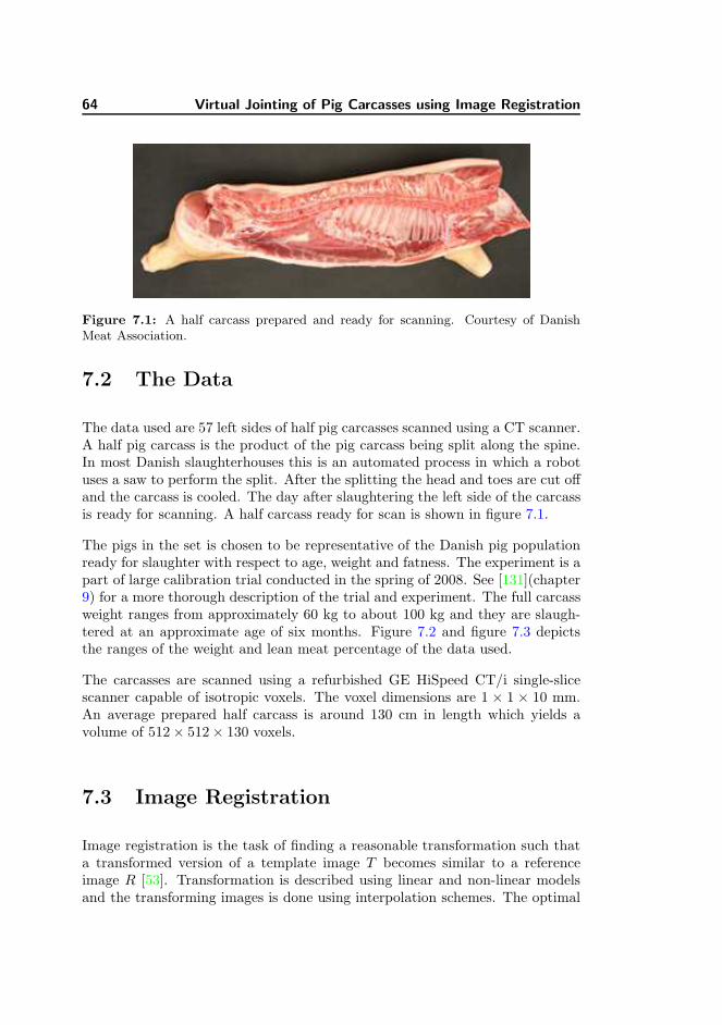
64 Virtual Jointing of Pig Carcasses using Image Registration

Figure 7.1: A half carcass prepared and ready for scanning. Courtesy of DanishMeat Association.

7.2 The Data

The data used are 57 left sides of half pig carcasses scanned using a CT scanner.A half pig carcass is the product of the pig carcass being split along the spine.In most Danish slaughterhouses this is an automated process in which a robotuses a saw to perform the split. After the splitting the head and toes are cut offand the carcass is cooled. The day after slaughtering the left side of the carcassis ready for scanning. A half carcass ready for scan is shown in figure 7.1.

The pigs in the set is chosen to be representative of the Danish pig populationready for slaughter with respect to age, weight and fatness. The experiment is apart of large calibration trial conducted in the spring of 2008. See [131](chapter9) for a more thorough description of the trial and experiment. The full carcassweight ranges from approximately 60 kg to about 100 kg and they are slaugh-tered at an approximate age of six months. Figure 7.2 and figure 7.3 depictsthe ranges of the weight and lean meat percentage of the data used.

The carcasses are scanned using a refurbished GE HiSpeed CT/i single-slicescanner capable of isotropic voxels. The voxel dimensions are 1 × 1 × 10 mm.An average prepared half carcass is around 130 cm in length which yields avolume of 512× 512× 130 voxels.

7.3 Image Registration

Image registration is the task of finding a reasonable transformation such thata transformed version of a template image T becomes similar to a referenceimage R [53]. Transformation is described using linear and non-linear modelsand the transforming images is done using interpolation schemes. The optimal

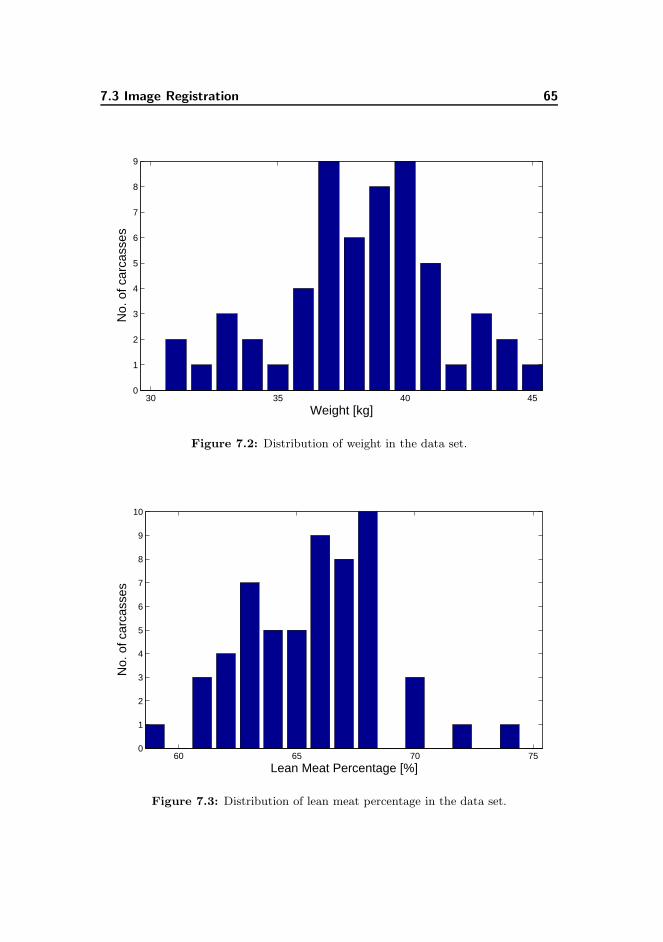
7.3 Image Registration 65

30 35 40 450

1

2

3

4

5

6

7

8

9

Weight [kg]

No.

of c

arca

sses

Figure 7.2: Distribution of weight in the data set.

60 65 70 750

1

2

3

4

5

6

7

8

9

10

Lean Meat Percentage [%]

No.

of c

arca

sses

Figure 7.3: Distribution of lean meat percentage in the data set.

66 Virtual Jointing of Pig Carcasses using Image Registration

transformation is described using some kind of similarity measure and findingit is the task of optimization. Adding a regularization term in the optimizationensures that the transformation is smooth.

7.3.1 Linear and Non-Linear Transformation Models

In this paper an image is seen as a continuous function defined on some domain.Sampling the continuous image on a grid of points enables the discretizationneeded. The sampling is done using an interpolation scheme. Many exist butin this paper a B-spline based scheme is used [120].

A grid is defined as a collection of grid points xi = (x1i , . . . , x

Di )⊤ for a D-

dimensional image. A 3D grid X of size n1 × n2 × n3 is defined as,

X =[

x1⊤ x2⊤ x3⊤]⊤

, (7.1)

where x1 =(

x11 . . . x

1N

)⊤, x2 =

(

x21 . . . x

2N

)⊤and x3 =

(

x31 . . . x

3N

)⊤, with

N = n1n2n3.

An image is transformed by transforming the underlying grid and then resam-pling the image. The transformation can be seen as a sum of an identity partand a deformation part,

y1i = x1i + u1(xi) (7.2)

y2i = x2i + u2(xi)

y3i = x3i + u3(xi),

where ud(xi) is the displacement of a grid point xi in the dth dimension.. Thusfor each grid point there is a corresponding displacement vector comprising avector field.

In image registration the images are usually preregistered using linear transfor-mations. In an atlas application it is desirable to remove effects from the imageacquisition process from the model. The most flexible linear transformation isthe affine transformation, which can model rotation, translation, scaling andshearing. The transformation of the entire grid X can be written as,

Y = X + I3 ⊗Qw, (7.3)

where I3 is a unit matrix of rank 3. The qijth element of Q is the evaluationof the jth basis function at the ith position. w is a vector of the parametersfor the corresponding basis functions. For the linear transformation the verysimple basis functions are,

q1 (xi) = x1i , q2 (xi) = x2

i , q3 (xi) = x3i , q4 (xi) = 1. (7.4)

7.3 Image Registration 67

A type of transformation capable of modeling non-linear deformations is basedon cubic B-splines [108]. As above the transformation can be written as a sumof basis functions,

ydi = xdi +

p1∑

j=1

p2∑

k=1

p3∑

l=1

bj(x1i )bk(x

2i )bl(x

3i )w

djkl , (7.5)

where p1,p2 and p3 are the number of equidistantly placed knots for the splines.Using the tensor product property of B-splines equation 7.5 can be written insimilar fashion as equation 7.3,

Y = X + I3 ⊗Q3 ⊗Q2 ⊗Q1w. (7.6)

Using a non-recursive definition [121] the following 1D cubic B-splines basisfunctions can be derived,

bj(xi) =

(2 + xi)3 for −2 ≤ xi < −1

−(3xi + 6)x2i + 4 for −1 ≤ xi < 0

(3xi − 6)x2i + 4 for 0 ≤ xi < 1

(2− xi)3 for 1 ≤ xi < 2

0 otherwise

(7.7)

7.3.2 Similarity and Optimization

The data in this paper consist of CT-scan of pig carcasses, and as such theregistration is between two intra-modal images. A similarity measure suited forthis situation is the sum-of-squared-differences (SSD) measure. It measures theEuclidean distance between grey values of corresponding voxels,

D(w) =h

2‖T (w)−R‖2, (7.8)

where h = h1h2h3 is the product of the voxel dimensions. A good choice foroptimization of SSD-problems is the Gauss-Newton algorithm. The basic ideais iteratively updating the parameters wk+1 = wk + sk by solving the linearsystem also known as the normal equations [93],

J⊤

k Jksk = −J⊤

k (T (Y )−R (X)) , (7.9)

where Jk is the Jacobian J(wk). Thus it only involves calculating the residualsand the Jacobian. In this parametric case the Jacobian can be written as,

Jk = ∇TQ =[

∇T 1∇T 2

∇T 3]

I3 ⊗Q3 ⊗Q2 ⊗Q1, (7.10)

where each∇T d is a diagonal matrix containing the partial derivatives ∂T (yi)/∂xd

of the image T .

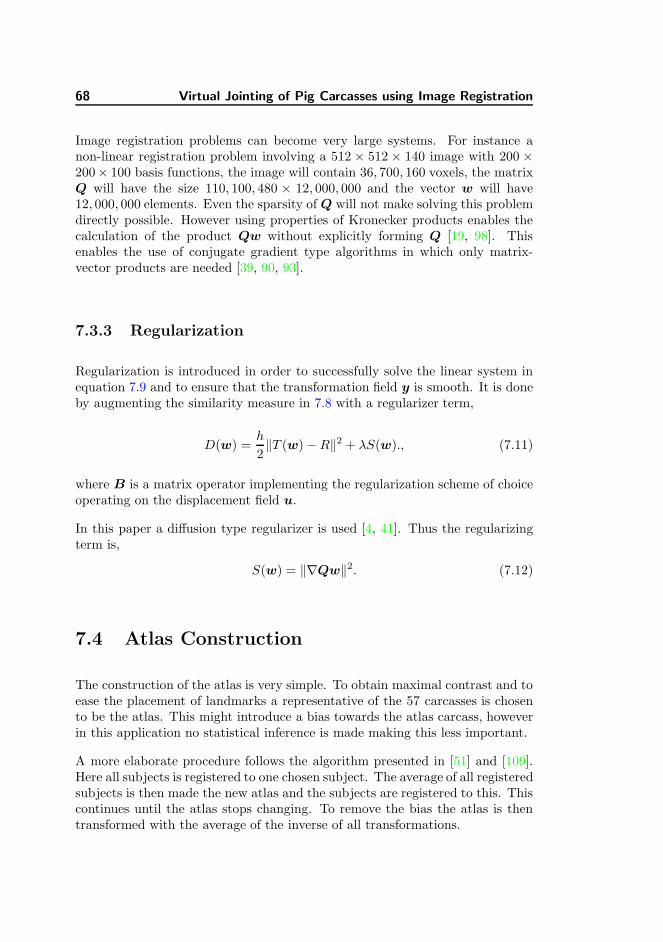
68 Virtual Jointing of Pig Carcasses using Image Registration

Image registration problems can become very large systems. For instance anon-linear registration problem involving a 512 × 512 × 140 image with 200 ×200× 100 basis functions, the image will contain 36, 700, 160 voxels, the matrixQ will have the size 110, 100, 480 × 12, 000, 000 and the vector w will have12, 000, 000 elements. Even the sparsity of Q will not make solving this problemdirectly possible. However using properties of Kronecker products enables thecalculation of the product Qw without explicitly forming Q [19, 98]. Thisenables the use of conjugate gradient type algorithms in which only matrix-vector products are needed [39, 90, 93].

7.3.3 Regularization

Regularization is introduced in order to successfully solve the linear system inequation 7.9 and to ensure that the transformation field y is smooth. It is doneby augmenting the similarity measure in 7.8 with a regularizer term,

D(w) =h

2‖T (w)−R‖2 + λS(w)., (7.11)

where B is a matrix operator implementing the regularization scheme of choiceoperating on the displacement field u.

In this paper a diffusion type regularizer is used [4, 41]. Thus the regularizingterm is,

S(w) = ‖∇Qw‖2. (7.12)

7.4 Atlas Construction

The construction of the atlas is very simple. To obtain maximal contrast and toease the placement of landmarks a representative of the 57 carcasses is chosento be the atlas. This might introduce a bias towards the atlas carcass, howeverin this application no statistical inference is made making this less important.

A more elaborate procedure follows the algorithm presented in [51] and [109].Here all subjects is registered to one chosen subject. The average of all registeredsubjects is then made the new atlas and the subjects are registered to this. Thiscontinues until the atlas stops changing. To remove the bias the atlas is thentransformed with the average of the inverse of all transformations.

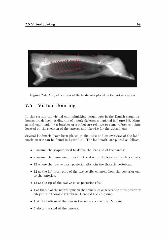
7.5 Virtual Jointing 69

Figure 7.4: A top-down view of the landmarks placed on the virtual carcass.

7.5 Virtual Jointing

In this section the virtual cuts mimicking actual cuts in the Danish slaughter-houses are defined. A diagram of a pork skeleton is depicted in figure 7.5. Manyactual cuts made by a butcher or a robot are relative to some reference pointslocated on the skeleton of the carcass and likewise for the virtual cuts.

Several landmarks have been placed in the atlas and an overview of the land-marks in use can be found in figure 7.4. The landmarks are placed as follows,

• 5 around the scapula used to define the fore-end of the carcass.

• 2 around the ilium used to define the start of the legs part of the carcass.

• 12 where the twelve most posterior ribs join the thoracic vertebrae.

• 12 at the left most part of the twelve ribs counted from the posterior endto the anterior.

• 12 at the tip of the twelve most posterior ribs.

• 1 at the tip of the neural spine in the same slice as where the most posteriorrib join the thoracic vertebrae. Denoted the P2 point.

• 1 at the bottom of the loin in the same slice as the P2 point.

• 5 along the rind of the carcass.

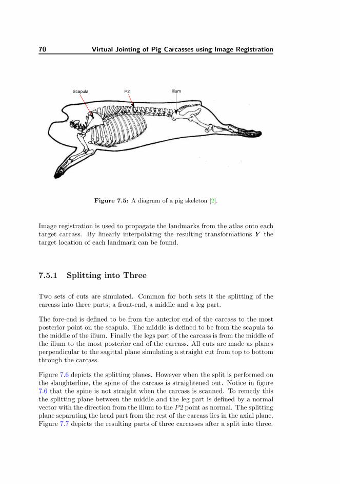
70 Virtual Jointing of Pig Carcasses using Image Registration

Figure 7.5: A diagram of a pig skeleton [2].

Image registration is used to propagate the landmarks from the atlas onto eachtarget carcass. By linearly interpolating the resulting transformations Y thetarget location of each landmark can be found.

7.5.1 Splitting into Three

Two sets of cuts are simulated. Common for both sets it the splitting of thecarcass into three parts; a front-end, a middle and a leg part.

The fore-end is defined to be from the anterior end of the carcass to the mostposterior point on the scapula. The middle is defined to be from the scapula tothe middle of the ilium. Finally the legs part of the carcass is from the middle ofthe ilium to the most posterior end of the carcass. All cuts are made as planesperpendicular to the sagittal plane simulating a straight cut from top to bottomthrough the carcass.

Figure 7.6 depicts the splitting planes. However when the split is performed onthe slaughterline, the spine of the carcass is straightened out. Notice in figure7.6 that the spine is not straight when the carcass is scanned. To remedy thisthe splitting plane between the middle and the leg part is defined by a normalvector with the direction from the ilium to the P2 point as normal. The splittingplane separating the head part from the rest of the carcass lies in the axial plane.Figure 7.7 depicts the resulting parts of three carcasses after a split into three.

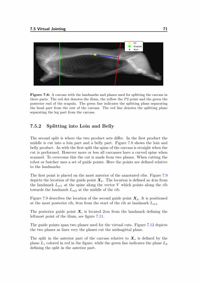
7.5 Virtual Jointing 71

P2ScapulaIlium

Figure 7.6: A carcass with the landmarks and planes used for splitting the carcass inthree parts. The red dot denotes the ilium, the yellow the P2 point and the green theposterior end of the scapula. The green line indicates the splitting plane separatingthe head part from the rest of the carcass. The red line denotes the splitting planeseparating the leg part from the carcass.

7.5.2 Splitting into Loin and Belly

The second split is where the two product sets differ. In the first product themiddle is cut into a loin part and a belly part. Figure 7.8 shows the loin andbelly product. As with the first split the spine of the carcass is straight when thecut is performed. However more or less all carcasses have a curved spine whenscanned. To overcome this the cut is made from two planes. When cutting therobot or butcher uses a set of guide points. Here the points are defined relativeto the landmarks.

The first point is placed on the most anterior of the annotated ribs. Figure 7.9depicts the location of the guide point Xr. The location is defined as 4cm fromthe landmark Lm1 at the spine along the vector V which points along the ribtowards the landmark Lm2 at the middle of the rib.

Figure 7.9 describes the location of the second guide point Xp. It is positionedat the most posterior rib, 8cm from the start of the rib at landmark Lm1.

The posterior guide point Xi is located 2cm from the landmark defining theleftmost point of the ilium, see figure 7.11.

The guide points span two planes used for the virtual cuts. Figure 7.12 depictsthe two planes as lines very the planes cut the midsagittal plane.

The split in the anterior part of the carcass relative to Xs is defined by theplane L1 colored in red in the figure, while the green line indicates the plane L2

defining the split in the anterior part.

72 Virtual Jointing of Pig Carcasses using Image Registration

Figure 7.7: The resulting parts after a split into three for three different carcasses.

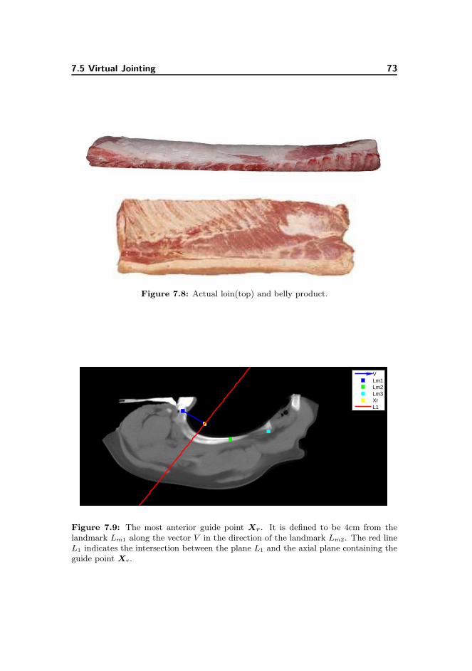
7.5 Virtual Jointing 73

Figure 7.8: Actual loin(top) and belly product.

VLm1Lm2Lm3XrL1

Figure 7.9: The most anterior guide point Xr. It is defined to be 4cm from thelandmark Lm1 along the vector V in the direction of the landmark Lm2. The red lineL1 indicates the intersection between the plane L1 and the axial plane containing theguide point Xr.

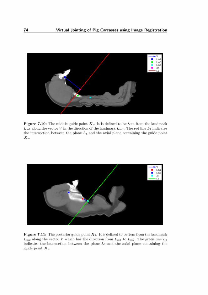
74 Virtual Jointing of Pig Carcasses using Image Registration

VLm1Lm2Lm3XsL1

Figure 7.10: The middle guide point Xs. It is defined to be 8cm from the landmarkLm1 along the vector V in the direction of the landmark Lm3. The red line L1 indicatesthe intersection between the plane L1 and the axial plane containing the guide pointXs.

VLm1Lm2XiL2

Figure 7.11: The posterior guide point Xi. It is defined to be 2cm from the landmarkLm2 along the vector V which has the direction from Lm1 to Lm2. The green line L2

indicates the intersection between the plane L2 and the axial plane containing theguide point Xi.

7.5 Virtual Jointing 75

XsL1XrL2XiN1N2

Figure 7.12: The two splitting planes defining the loin part.

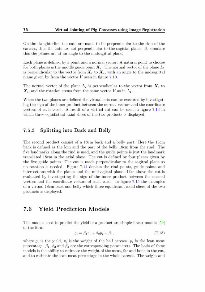
76 Virtual Jointing of Pig Carcasses using Image Registration

On the slaughterline the cuts are made to be perpendicular to the skin of thecarcass, thus the cuts are not perpendicular to the sagittal plane. To simulatethis the planes are at an angle to the midsagittal plane.

Each plane is defined by a point and a normal vector. A natural point to choosefor both planes is the middle guide point Xs. The normal vector of the plane L1

is perpendicular to the vector from Xr to Xs, with an angle to the midsagittalplane given by from the vector V seen in figure 7.10.

The normal vector of the plane L2 is perpendicular to the vector from Xs toXi, and the rotation stems from the same vector V as in L1.

When the two planes are defined the virtual cuts can be executed by investigat-ing the sign of the inner product between the normal vectors and the coordinatevectors of each voxel. A result of a virtual cut can be seen in figure 7.13 inwhich three equidistant axial slices of the two products is displayed.

7.5.3 Splitting into Back and Belly

The second product consist of a 18cm back and a belly part. Here the 18cmback is defined as the loin and the part of the belly 18cm from the rind. Thefive landmarks along the rind is used, and the guide points is just the landmarktranslated 18cm in the axial plane. The cut is defined by four planes given bythe five guide points. The cut is made perpendicular to the sagittal plane sono rotation is needed. Figure 7.14 depicts the rind points, guide points andintersections with the planes and the midsagittal plane. Like above the cut isevaluated by investigating the sign of the inner product between the normalvectors and the coordinate vectors of each voxel. In figure 7.15 the examplesof a virtual 18cm back and belly which three equidistant axial slices of the twoproducts is displayed.

7.6 Yield Prediction Models

The models used to predict the yield of a product are simple linear models [59]of the form,

gi = β1vi + β2pi + β3, (7.13)

where gi is the yield, vi is the weight of the half carcass, pi is the lean meatpercentage. β1, β2 and β3 are the corresponding parameters. The basis of thesemodels is the ability to estimate the weight of the meat, fat and bone in the cut,and to estimate the lean meat percentage in the whole carcass. The weight and

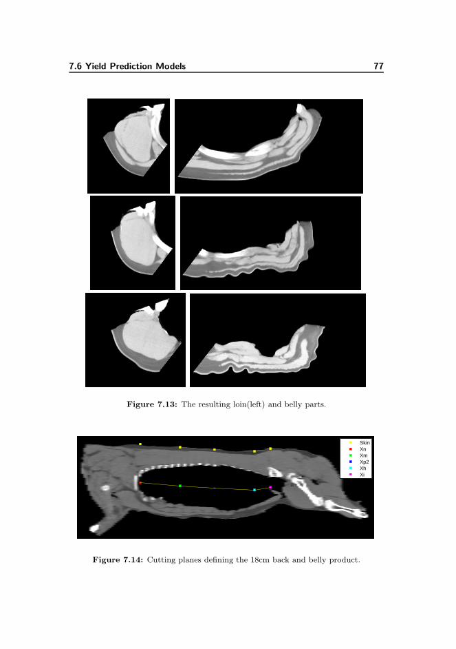
7.6 Yield Prediction Models 77

Figure 7.13: The resulting loin(left) and belly parts.

SkinXnXmXp2XhXi

Figure 7.14: Cutting planes defining the 18cm back and belly product.

78 Virtual Jointing of Pig Carcasses using Image Registration

Figure 7.15: The resulting back(left) and belly parts.

7.7 Results 79

the lean meat percentage is estimated from the CT volume data using linearmodel based on a pixel classification algorithm described in [131](see chapter9).

7.7 Results

All 57 carcasses are registered to an atlas chosen as a carcass representative of thepopulation. Each carcass volume is resampled to a volume size of 512×256×192voxels. For the non-linear part of the registration the basis functions are placed20, 10 and 5mm apart for the coarse to fine level respectively. Six differentregistrations are performed on each of the 24 carcasses correspond to six levels ofthe regularizing parameter λ. The values are λi =

[

10−2, 10−1, 100, 101, 102, 103]

for i = 1 . . . 6.

7.7.1 Choice of Regularization Parameter

In order to determine the optimal value for the regularization parameter twoquantitative measures are used.

One quantitative measure is based on landmarks. 24 carcasses was selected andannotated using nine of the landmarks described in the scheme described insection 7.5. The landmarks are the five around the scapula, the two around theilium, the P2 point and the loin point. The landmarks are used to evaluate theregistration accuracy by measuring the Euclidean distance between the auto-matically placed and its corresponding manually placed. Basically, the metricis a sum over 24 Euclidean distances in carcass j,

Dlmj =

1

9

9∑

i=1

‖φ(xri)− xti‖2 =

1

9

9∑

i=1

‖xri + u(xri)− xt‖2, (7.14)

where xti is the manually placed landmark i, xri is the corresponding prop-agated landmark. u(xr) is the displacement in xr and is found by linearlyinterpolating the resulting displacement field U = Y − X. As a score for aparticular value of the regularization parameter is the average landmark error,

Dlmλ =

1

24

2∑

i=1

4Dlmj , (7.15)

The left plot in figure 7.16 depicts a the mean and standard deviation of theEuclidean distances.

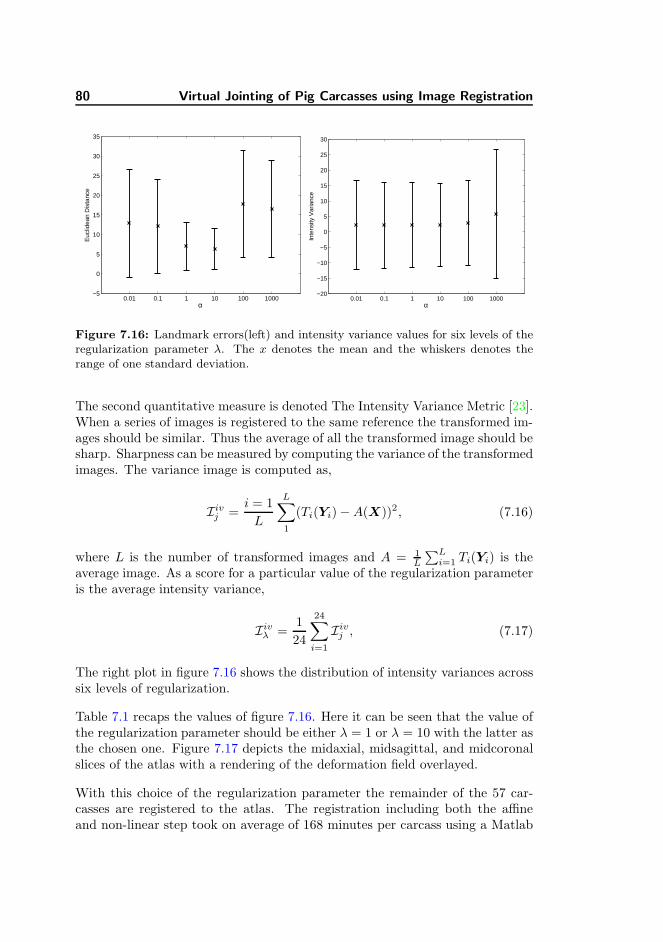
80 Virtual Jointing of Pig Carcasses using Image Registration

0.01 0.1 1 10 100 1000−5

0

5

10

15

20

25

30

35

α

Euc

lidea

n D

ista

nce

0.01 0.1 1 10 100 1000−20

−15

−10

−5

0

5

10

15

20

25

30

αIn

tens

ity V

aria

nce

Figure 7.16: Landmark errors(left) and intensity variance values for six levels of theregularization parameter λ. The x denotes the mean and the whiskers denotes therange of one standard deviation.

The second quantitative measure is denoted The Intensity Variance Metric [23].When a series of images is registered to the same reference the transformed im-ages should be similar. Thus the average of all the transformed image should besharp. Sharpness can be measured by computing the variance of the transformedimages. The variance image is computed as,

Iivj =i = 1

L

L∑

1

(Ti(Yi)−A(X))2, (7.16)

where L is the number of transformed images and A = 1L

∑Li=1 Ti(Yi) is the

average image. As a score for a particular value of the regularization parameteris the average intensity variance,

Iivλ =1

24

24∑

i=1

Iivj , (7.17)

The right plot in figure 7.16 shows the distribution of intensity variances acrosssix levels of regularization.

Table 7.1 recaps the values of figure 7.16. Here it can be seen that the value ofthe regularization parameter should be either λ = 1 or λ = 10 with the latter asthe chosen one. Figure 7.17 depicts the midaxial, midsagittal, and midcoronalslices of the atlas with a rendering of the deformation field overlayed.

With this choice of the regularization parameter the remainder of the 57 car-casses are registered to the atlas. The registration including both the affineand non-linear step took on average of 168 minutes per carcass using a Matlab

7.7 Results 81

λ 0.01 0.1 1 10 100 1000

Dlmλ [mm] 12.8 12.1 7.0 6.3 17.7 16.4Iivλ 2.2 2.1 2.1 2.2 2.7 5.8

Table 7.1: The average landmark and intensity variance for six levels of regularization.

β1 β2 β3

Loin 0.0005 [−0.0005 0.0016] 0.0131 [0.0119 0.0142] −0.1423 [−0.2332 − 0.0514]Back −0.0002 [−0.0013 0.0008] 0.0148 [0.0137 0.0159] −0.2828 [−0.3716 − 0.1939]

Table 7.2: Parameters of the yield prediction models for the loin and 18cm backproducts.

implementation on a 64bit PC with 4 dual core AMD 1.8GHz processors, and32GB RAM.

7.7.2 Virtual Cuts

After registration of each of the 57 carcasses the virtual cuts are performed.Each carcass is cut into three parts; a front end, a middle end and the legs.The middle is then cut into a loin and belly product and a 18cm back and bellyproduct. The cuts are made as described in section 7.5. A qualitative estimationof the cuts are made by visual inspection of the results. Examples of the virtualcuts can be seen in section 7.9.1

7.7.3 Yield Prediction Models

The main goal of this study is to predict the yield of the loin and the 18cmback product using virtual cuts. Yield is defined as the fraction of meat in theproduct. This is calculated as the weight of the meat divided by the weight ofthe product. The weight of the bones in the product is not included. A modelas described in equation 7.13 is fitted to the calculated yield of the loin andback. The results are seen in table 7.2. The total carcass weight is found tobe not significant and is subsequently left out. Histograms of the weight andlean meat percentages used as input are depicted in figures 7.2 and 7.3. Table7.3 shows the parameters for an reduced model containing only the lean meatpercentage as predictor. The model has an explained variance of R2 = 0.90 andR2 = 0.93 of loin and 18cm back yield respectively. Figure 7.18 shows the fit ofthe models to the data.

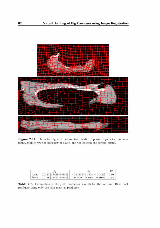
82 Virtual Jointing of Pig Carcasses using Image Registration

Figure 7.17: The atlas pig with deformation fields. Top row depicts the midaxialplane, middle row the midsagittal plane, and the bottom the coronal plane.

β2 β3 R2

Loin 0.0130 [0.0119 0.0141] −0.1169 [−0.1924 − 0.0413] 0.90Back 0.0148 [0.0137 0.0159] −0.2929 [−0.3661− 0.2196] 0.93

Table 7.3: Parameters of the yield prediction models for the loin and 18cm backproducts using only the lean meat as predictor.

7.7 Results 83

58 60 62 64 66 68 70 72 74 76

0.65

0.7

0.75

0.8

0.85

0.9

0.95

Lean Meat Percentage

Loin

Yie

ld

0 10 20 30 40 50 60−0.04

−0.03

−0.02

−0.01

0

0.01

0.02

0.03

Carcass ID

Res

idua

l Loi

n Y

ield

58 60 62 64 66 68 70 72 74 760.55

0.6

0.65

0.7

0.75

0.8

0.85

0.9

Lean Meat Percentage

Bac

k Y

ield

0 10 20 30 40 50 60−0.025

−0.02

−0.015

−0.01

−0.005

0

0.005

0.01

0.015

0.02

0.025

Carcass ID

Res

idua

l Bac

k Y

ield

Figure 7.18: The left plot depicts yield of the loin(top) and the 18cm back vs. thelean meat percentage. The right plot depicts the residuals when predicting the yield.

84 Virtual Jointing of Pig Carcasses using Image Registration

7.8 Discussion and Conclusion

This paper present a preliminary study in the use of CT as a tool for the pre-diction of yield in cuts of a pig carcass. The errors of the virtual cuts made onthe carcasses depend on a number of factors. One important cause of error is ofcourse the registration accuracy. This is measured using the landmarks with amean Euclidean distance in the training set. This best result is reported to beDlm = 6.3mm which is acceptable bearing in mind that the voxel dimension is1×1×10. Furthermore considering the voxel dimensions the placing of the land-marks is very error prone. A measure of the uncertainty of the landmarks is notobtained but by using multiple experts to annotate and following [11, 95] thisis clearly possible and should be done in further studies. The effect of misalign-ment due to registration inaccuracy and landmark errors on the yield estimateshould also be investigated. Other more elaborate methods of landmark locat-ing schemes, such as feature detection methods or segmentation based methods,could also have been chosen. However, the choice of image registration has twodistinct advantages. One is the ability to process a whole batch of carcasses oncethe registration has been performed, and the other is that the set of landmarksor segmentation can be altered in the atlas without the need for a new set ofregistrations. This enables the implementation of other cuts rather quickly.

In this preliminary study the cuts defined are not real-life cuts but rather anadaptation. In further studies the actual definitions of the various cuts must beimplemented, however such knowledge is considered proprietary by the slaugh-terhouses and not suitable for publication.

The prediction models based solely on the lean meat percentage show acceptableresults. However a comparison with actual cuts made by a trained butcher orrobot is needed in order to access the validity of the results.

All in all the study shows potential for the use of CT and image registrationas means for the automatic non-invasive prediction of yield in commercial cutsof pig carcasses. It is possible to calibrate the sorting models presently used inthe slaughterhouses with a much larger quantity of carcasses than it is today.But also the search of other predictors such as fat layer thickness etc. is muchmore feasible using this method. However, ultimately the success of this methoddepends on how accurately real-life cuts can be modeled.

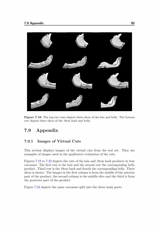
7.9 Appendix 85

Figure 7.19: The top two rows depicts three slices of the loin and belly. The bottomrow depicts three slices of the 18cm back and belly.

7.9 Appendix

7.9.1 Images of Virtual Cuts

This section displays images of the virtual cuts from the test set. They areexamples of images used in the qualitative evaluation of the cuts.

Figures 7.19 to 7.22 depicts the cuts of the loin and 18cm back products in fourcarcasses. The first row is the loin and the second row the corresponding bellyproduct. Third row is the 18cm back and fourth the corresponding belly. Threeslices is shown. The images in the first column is from the middle of the anteriorpart of the product, the second column is the middle slice and the third is fromthe posterior part of the product.

Figure 7.23 depicts the same carcasses split into the three main parts.

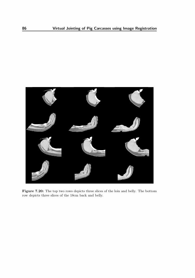
86 Virtual Jointing of Pig Carcasses using Image Registration

Figure 7.20: The top two rows depicts three slices of the loin and belly. The bottomrow depicts three slices of the 18cm back and belly.

7.9 Appendix 87

Figure 7.21: The top two rows depicts three slices of the loin and belly. The bottomrow depicts three slices of the 18cm back and belly.

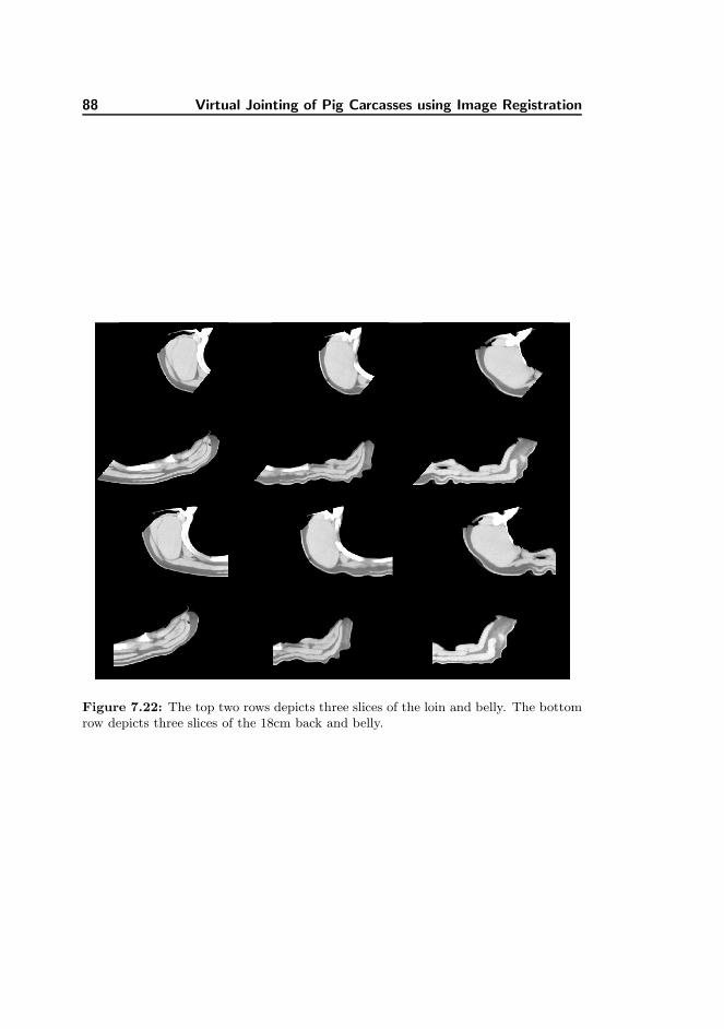
88 Virtual Jointing of Pig Carcasses using Image Registration

Figure 7.22: The top two rows depicts three slices of the loin and belly. The bottomrow depicts three slices of the 18cm back and belly.

7.9 Appendix 89

Figure 7.23: Three carcasses split into three parts.

90 Virtual Jointing of Pig Carcasses using Image Registration

Part IV

Contributions

Chapter 8

Robustness of weight and

meat content in pigs

determined by CT

L.B. Christensen, M. Vester-Christensen, C. Borggaard and E.V. Olsen

Abstract

An increasing number of European countries are exploring the applica-tion of computer tomography (CT) as objective reference technology fordetermination of lean meat percentage (LMP) in domestic animals. Oneimportant requirement for a reference is the reproducibility or quantitativeperformance. 23 carcasses are CT scanned twice using different settings.The first setting was equal for all carcasses (140 kV, 140 mA, helical, stan-dard reconstruction) whereas for the second scanning either photon current,reconstruction algorithm, or physical position of carcass was changed. Theweight determination was based on a volumetric method using specific con-stants for lean meat, fat and bone tissue thus leaving any difference to be avolume issue. The lean meat content was a simple calculation based on thetissue weights. Our results on weight determination showed that the softreconstruction algorithm overestimated the weight of the carcass by 0.3%compared to the standard reconstruction. The reduction of photon currentdown to 80 mA or repositioning of the carcass showed no significant influ-ence on the weight. When calculating LMP no of the introduced changes

94 Robustness of weight and meat content in pigs determined by CT

in CT protocol introduced significant effect on the estimate of LMP , thusleaving CT as a very robust reference method for determination of LMP

in pigs.

8.1 Introduction

Estimation of the lean meat percentage (LMP ) is a central part of determina-tion the value of a pig carcass. It is important to the farmer as he is paid bycarcass weight and LMP , it is important to the abattoir as the final productionyield is influenced by the LMP and an important sorting procedure based onLMP is often employed to optimize the yield. As carcass payment is underEU-regulation objectivity and transparency of the reference for the estimationprocess is of major importance. Today the reference is based on a manually dis-section of commercially important parts of the carcass and thereby the referenceis influenced by operator skills and cutting tradition [38]. One way of copingwith this problem is to apply a virtual dissection to the carcasses using a full-body CT scanning and a software tool to estimate the LMPCT of the individualcarcass. Two different strategies to determine the LMPCT has been proposed:A spectral calibration where the distribution of all voxel densities measured onthe Hounsfield scale is calibrated to the result of a manual dissection processusing multivariate models. This procedure includes the cutting tradition in thecalibration [38]. One other strategy is based on contextual volume grading ofall voxels into three different tissue classes: fat, meat or bone [84] The latterhas the important advantage of not being influenced by cut-ting tradition noroperator skills. Therefore we apply this strategy.

8.2 Material and Methods

23 pig carcasses was CT scanned twice using two different settings of the CTscanner (GE HiSpeed CT/i) The carcasses were 24 hours PM, prepared fora manual dissection according to EU recommendation, i.e. cutting the headand the feet and removing eventually internal fat and spine cord remains. Thescanning was performed twice in a chilled laboratory temporarily attached tothe cooling room of the abattoir. One first scanning protocol was used for allcarcasses and one second protocol was changed with respect to one of threedifferent scanning parameters according to table 1. The constant protocol pa-rameters are: 140kV volt-age, 0.9×0.9×10mm voxel size, 0.7 mm spot size and10 mm between slice centers. The scanned tomograms were analyzed with acontextual based Markov Random Fields type of algorithm called Owen-Hjort-Mohn [84]. The algorithm estimates the volume of lean meat, fat and bone

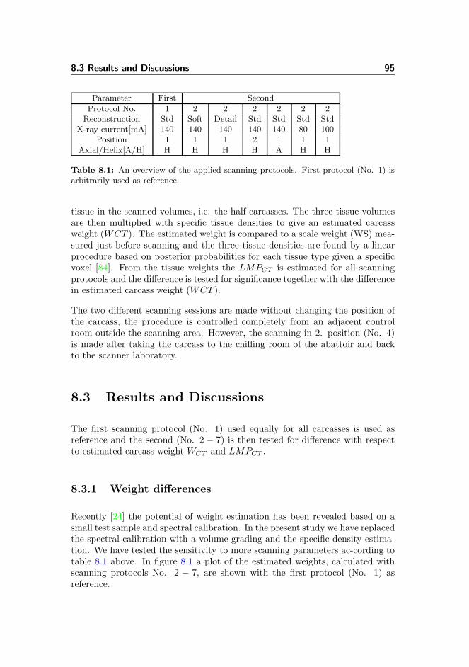
8.3 Results and Discussions 95

Parameter First Second

Protocol No. 1 2 2 2 2 2 2Reconstruction Std Soft Detail Std Std Std Std

X-ray current[mA] 140 140 140 140 140 80 100Position 1 1 1 2 1 1 1

Axial/Helix[A/H] H H H H A H H

Table 8.1: An overview of the applied scanning protocols. First protocol (No. 1) isarbitrarily used as reference.

tissue in the scanned volumes, i.e. the half carcasses. The three tissue volumesare then multiplied with specific tissue densities to give an estimated carcassweight (WCT ). The estimated weight is compared to a scale weight (WS) mea-sured just before scanning and the three tissue densities are found by a linearprocedure based on posterior probabilities for each tissue type given a specificvoxel [84]. From the tissue weights the LMPCT is estimated for all scanningprotocols and the difference is tested for significance together with the differencein estimated carcass weight (WCT ).

The two different scanning sessions are made without changing the position ofthe carcass, the procedure is controlled completely from an adjacent controlroom outside the scanning area. However, the scanning in 2. position (No. 4)is made after taking the carcass to the chilling room of the abattoir and backto the scanner laboratory.

8.3 Results and Discussions

The first scanning protocol (No. 1) used equally for all carcasses is used asreference and the second (No. 2 − 7) is then tested for difference with respectto estimated carcass weight WCT and LMPCT .

8.3.1 Weight differences

Recently [24] the potential of weight estimation has been revealed based on asmall test sample and spectral calibration. In the present study we have replacedthe spectral calibration with a volume grading and the specific density estima-tion. We have tested the sensitivity to more scanning parameters ac-cording totable 8.1 above. In figure 8.1 a plot of the estimated weights, calculated withscanning protocols No. 2 − 7, are shown with the first protocol (No. 1) asreference.

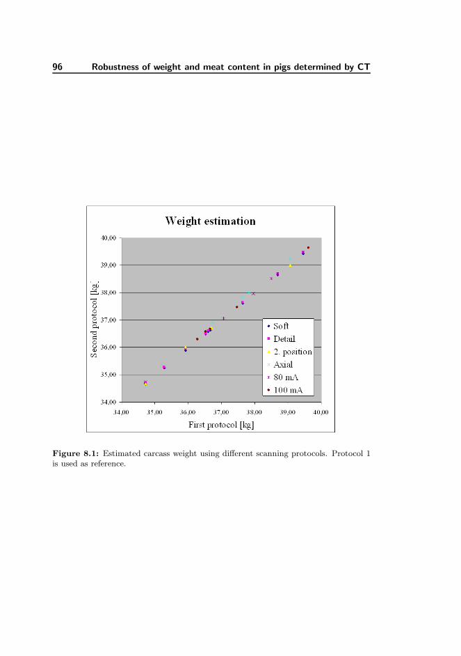
96 Robustness of weight and meat content in pigs determined by CT

Figure 8.1: Estimated carcass weight using different scanning protocols. Protocol 1is used as reference.

8.4 Conclusion 97

Protocol difference Soft Detail 2.position Axial 80 mA 100 mA

Protocol No. 2 3 4 5 6 7Difference [kg] 0.041 0.007 0.001 −0.18 −0.009 −0.017Difference [%] 0.11 0.02 0.00 −0.48 −0.03 −0.05Significance p 0.0000 0.0570 0.9761 0.0000 0.0209 0.0955

Significance level *** NS NS *** * NS

Table 8.2: Weight estimation.

Protocol difference Soft Detail 2.position Axial 80 mA 100 mA

Protocol No. 2 3 4 5 6 7Difference [LMPCT %] −0.02 0.03 −0.10 0.17 −0.05 0.04

Significance p 0.3108 0.1285 0.2620 0.0074 0.1990 0.2943Significance level NS NS NS ** NS NS

Table 8.3: LMPCT estimation.

The average difference between weight estimates from the first protocol to thesecond protocol is calculated and tested using a standard t-test. The resultsshow a significant difference in weight estimate of less than 0.5% irrespective ofwhich of the seven different scanning protocols that is applied to the scanningprocedure. This is of the same level as estimated for the used scale.

8.3.2 LMPCT estimation

The sensitivity of the LMPCT estimation to the scanning protocol is evaluatedand the results shown in figure 8.2. The correlation seems even better thanthe performance for the weight estimation. Again the difference between theLMPCT estimated with the different scanning protocols of table 1 is evaluatedand tested for significant difference using a standard t-test. The results listed intable 8.3 show that LMPCT estimation only has a slight dependence (∗∗) of thechanges in scanning protocol applied in this experiment. The most significantdifference is the change of Helix to Axial scanning where a difference (p = 0.0074)is found.

8.4 Conclusion

From this experiment it may be deduced that CT is capable of measuring carcassweight and estimate the lean meat content in a quite robust and objective way.The highest sensitivity of scanning protocol is found in weight estimation wherea relative error of less than 0.5% of changing a Helix scanning to an Axial

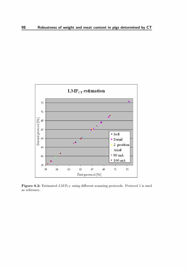
98 Robustness of weight and meat content in pigs determined by CT

Figure 8.2: Estimated LMPCT using different scanning protocols. Protocol 1 is usedas reference.

8.5 Acknowledgements 99

scanning protocol. Minor sensitivity (but still significant) is found by change ofreconstruction algorithm from a standard to a soft and no significance influencein repositioning the carcass, reduction of photon current from 140 mA to 100mA or reconstruction with a high contrast detailed algorithm. Determinationof the lean meat content, expressed as LMPCT , is demonstrated to be even lesssensitive to the imposed changes in scanning protocol. For estimation of thisvery important parameter the experiment reveals that CT may be expected tohave only a slight dependence to changing the scanning from Helix to Axial.The remaining changes in reconstruction, positioning and applied x-ray currentresult in not significant changes in the LMPCT determination. This concludesthat CT offers a robust measurement technology with a very small sensitivityto the different settings of the scanning protocol.

8.5 Acknowledgements

We thank our colleagues Jesper Blom-Hansen, Mads Fogtmann Hansen, SørenHemmingsen Erbou and Peter Vorup for their dedication and attention to detailin this experiment.

100 Robustness of weight and meat content in pigs determined by CT

Chapter 9

Virtual Dissection of Pig

Carcasses

Martin Vester-Christensen, Søren G. H. Erbou, Mads F. Hansen, Eli V. Olsen,

Lars B. Christensen, Marchen Hviid, Bjarne K. Ersbøll and Rasmus Larsen

Abstract

This paper proposes the use of computed tomography (CT) as a referencemethod for estimating the lean meat percentage (LMP) of pig carcasses.The current reference is manual dissection which has a limited accuracydue to variability between butchers. A contextual Bayesian classificationscheme is applied to classify volume elements of full body CT-scans of pigcarcasses into three tissue types. A linear model describes the relationbetween voxels and the full weight of the half carcass, which can be deter-mined more accurately than that of the lean meat content. 299 half pigcarcasses were weighed and CT-scanned. The explained variance of themodel was R

2 = 0.9994 with a root mean squared error of prediction of83.6g. Applying this method as a reference will ensure a more robust cali-bration of sensors for measuring the LMP, which is less prone to variationinduced by manual intervention.

9.1 Introduction

Throughout the European Union (EU) the lean meat percentage (LMP) is usedfor classifying pig carcasses and is defined as the ratio of weighed lean meatversus the weight of the pig carcass. Measuring the LMP is typically done usingultrasound or optical sensors which are calibrated towards a common manualdissection method of half pig carcasses, cf. Commission of the European Com-munities (EC) [27] and Walstra and Merkus [134]. The accuracy and precision

102 Virtual Dissection of Pig Carcasses

of these calibrations are limited by that of the dissection method. Only highlytrained butchers are involved in such a dissection. Even so there is still a signifi-cant difference between butchers as reported by Nissen et al. [92]. The maximumdifference in estimated LMP between 8 butchers is found to be 1.96 LMP unitsand the jointing of the carcasses is found to be a critical point in the EU dissec-tion method. Furthermore variation between countries were also found. Olsenet al. [97] report that in general variations between butchers is more importantthan variations between copies of the same type of instrument, when calibratinginstruments to manual dissection.

X-ray computed tomography (CT), cf. Cho et al. [21], is a non-invasive tech-nique that measures the radio-density of a material, i.e. the relative attenuationof X-rays through the material and is measured in the Hounsfield scale. Thescale is calibrated such that air is at −1000 Hounsfield Units (HU) and waterat 0HU, making HU-values comparable across scanners and settings. Fat tissueis usually around −60HU, meat tissue around +60HU and bone tissue above∼ 150HU. The CT-volume consists of discrete volume elements (voxels) and arenot necessarily isotropic. Voxels might also consist of more than one class oftissue. The latter is denoted partial volume effects (PVE) and results in over-lapping probability density functions (pdf) of the different tissues. Figure 9.1shows a typical histogram in the fat/meat range for a CT scanned pig carcass.The left peak represents fat and the right peak represents meat. Bone is abovethe range shown.

The fixed Hounsfield scale of CT is a major reason for using CT instead of mag-netic resonance imaging (MRI) because it is comparable across scanners. Ap-plying different settings, or protocols, in a specific CT-scanner has been shownby Christensen et al. [23] to give quite robust results w.r.t. LMP. Based on 23pig carcasses and using 7 different protocols they find a maximum difference of0.27 LMP units and a maximum difference in the estimated carcass weight of0.22kg.

Typically a simple threshold in the CT histogram is used to distinguish fat,meat and bone tissue, but this will often result in errors caused by noise in thereconstruction, artifacts and PVE.

Several attempts have been made on calibration of CT scans of pigs carcasses topredict the lean meat content of manual dissections. Glasbey and Robinson [46]derive and compare estimators of tissue volumes in CT images taking mixed pix-els, or PVE, of fat and meat into account. A moment-based estimator performsbest in both a simulation study and in a particular application where tissuecomposition of sheep is estimated. The improvement in precision is reported tobe minor compared to Cavalieri sampling, cf. Roberts et al. [101].

Dobrowolski et al. [34] and Romvari et al. [106] use thresholds in the histogram

9.1 Introduction 103

−150 −100 −50 0 50 100 150Hounsfield Units [HU]

Figure 9.1: Histogram of a CT-volume of a pig carcass. The ordinate is scaled toshow the distribution of fat (left) and meat voxels (right).

of CT and Collewet et al. [25] of MRI scans to segment meat voxels. In thesestudies partial least-squares regression (PLSR) of histogram values is applied tomodel the dissected lean meat content. Table 9.1 summarizes their results alongwith those of Johansen et al. [68]. R2 is the explained variance and RMSEP/Care the root mean squared errors of prediction/calibration. Johansen et al. [68]apply thresholds to the histogram of 15 anatomically chosen slices of 120 CT-scanned carcasses of lamb to segment fat and meat tissue. A multidimensionalPLS model is applied on the histogram values of fat and meat to predict thecorresponding weights in a manual dissection. The RMSEP of the meat contentis reported to be 772g before and 561g after bias correction, with an R2 = 0.96.Common for the above mentioned methods is that they only take into accountthe histogram value of the voxel to be classified and not any of the neighboringvoxels.

Lyckegaard et al. [84] apply a multivariate Bayesian 2D contextual classifica-tion scheme to each slice as described by Larsen [78]. Certain combinations ofneighboring voxels are taken into account modeled in a Bayesian scheme withpriors obtained from thresholds in the histogram. Linear regression is used toestimate the parameters of a model mapping the volume of fat, meat and boneto the total weight of the carcass, with an R2 = 0.991 and a RMSEP= 584g.

This paper presents an experiment consisting of 299 pig carcasses, which areweighed and CT-scanned. Applying methods from image processing along witha contextual classification scheme the CT-volume is classified into several typesof tissue. A linear model determines the mapping from voxels to the full weightof the half carcass, which is then used for estimating the CT-based LMP.

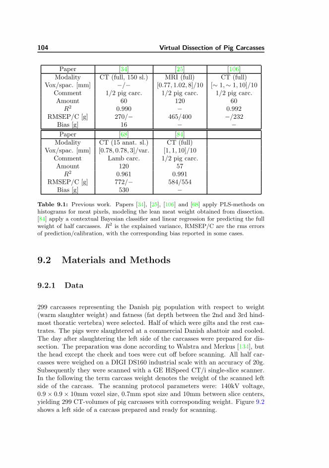
104 Virtual Dissection of Pig Carcasses

Paper [34] [25] [106]Modality CT (full, 150 sl.) MRI (full) CT (full)

Vox/spac. [mm] −/− [0.77, 1.02, 8]/10 [∼ 1,∼ 1, 10]/10Comment 1/2 pig carc. 1/2 pig carc. 1/2 pig carc.Amount 60 120 60

R2 0.990 − 0.992RMSEP/C [g] 270/− 465/400 −/232

Bias [g] 16 − −

Paper [68] [84]Modality CT (15 anat. sl.) CT (full)

Vox/spac. [mm] [0.78, 0.78, 3]/var. [1, 1, 10]/10Comment Lamb carc. 1/2 pig carc.Amount 120 57

R2 0.961 0.991RMSEP/C [g] 772/− 584/554

Bias [g] 530 −

Table 9.1: Previous work. Papers [34], [25], [106] and [68] apply PLS-methods onhistograms for meat pixels, modeling the lean meat weight obtained from dissection.[84] apply a contextual Bayesian classifier and linear regression for predicting the fullweight of half carcasses. R

2 is the explained variance, RMSEP/C are the rms errorsof prediction/calibration, with the corresponding bias reported in some cases.

9.2 Materials and Methods

9.2.1 Data

299 carcasses representing the Danish pig population with respect to weight(warm slaughter weight) and fatness (fat depth between the 2nd and 3rd hind-most thoratic vertebra) were selected. Half of which were gilts and the rest cas-trates. The pigs were slaughtered at a commercial Danish abattoir and cooled.The day after slaughtering the left side of the carcasses were prepared for dis-section. The preparation was done according to Walstra and Merkus [134], butthe head except the cheek and toes were cut off before scanning. All half car-casses were weighed on a DIGI DS160 industrial scale with an accuracy of 20g.Subsequently they were scanned with a GE HiSpeed CT/i single-slice scanner.In the following the term carcass weight denotes the weight of the scanned leftside of the carcass. The scanning protocol parameters were: 140kV voltage,0.9 × 0.9× 10mm voxel size, 0.7mm spot size and 10mm between slice centers,yielding 299 CT-volumes of pig carcasses with corresponding weight. Figure 9.2shows a left side of a carcass prepared and ready for scanning.

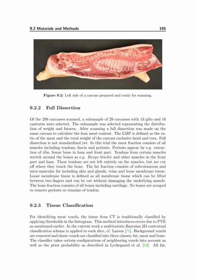
9.2 Materials and Methods 105

Figure 9.2: Left side of a carcass prepared and ready for scanning.

9.2.2 Full Dissection

Of the 299 carcasses scanned, a subsample of 29 carcasses with 13 gilts and 16castrates were selected. The subsample was selected representing the distribu-tion of weight and fatness. After scanning a full dissection was made on thesame carcass to calculate the lean meat content. The LMP is defined as the ra-tio of the meat and the total weight of the carcass exclusive head and toes. Fulldissection is not standardized yet. In this trial the meat fraction consists of allmuscles including tendons, fascia and periosts. Periosts appear by e.g. extrac-tion of ribs, femur bone in ham and front part. Tendons from certain musclesstretch around the bones as e.g. Biceps brachii and other muscles in the frontpart and ham. These tendons are not left entirely on the muscles, but are cutoff where they touch the bone. The fat fraction consists of subcutaneous andinter-muscular fat including skin and glands, veins and loose membrane tissue.Loose membrane tissue is defined as all membrane tissue which can be liftedbetween two fingers and can be cut without damaging the underlying muscle.The bone fraction consists of all bones including cartilage. No bones are scrapedto remove periosts or remains of tendon.

9.2.3 Tissue Classification

For identifying meat voxels, the tissue from CT is traditionally classified byapplying thresholds in the histogram. This method introduces errors due to PVEas mentioned earlier. In the current work a multivariate Bayesian 2D contextualclassification scheme is applied to each slice, cf. Larsen [78]. Background voxelsare removed and tissue voxels are classified into three classes; fat, meat and bone.The classifier takes certain configurations of neighboring voxels into account aswell as the prior probability as described in Lyckegaard et al. [84]. All fat,

106 Virtual Dissection of Pig Carcasses

meat and bone tissue irrespective of their anatomical position are regarded asbelonging to the same corresponding class. As a postprocessing step the bonesare morphologically closed such that marrow will be part of the bone class. InCT skin voxels are more similar to meat. When comparing the LMP obtained byCT to that obtained by manual dissection the skin is segmented separately andconsidered as fat such that the LMP can be computed according to Commissionof the European Communities (EC) [27]. Segmentation of the skin is done usingmathematical morphology, cf. Gonzalez and Woods [48].

9.2.4 Density Estimation

Estimating the weight of a carcass requires an approximation of the densitiesρ of the tissue types in every voxel. The carcass weight is modeled as a linearcombination of the weights of the tissue classes. Labeling of a particular voxelis done by choosing the class with maximum a posteriori (MAP) probability,see Larsen [78]. The MAP model applied for a single carcass with three tissueclasses is,

wi = ρfnfv + ρmnmv + ρbnbv + ǫi, (9.1)

where v is the voxel volume, nf , nm and nb are the number of voxels classifiedas fat, meat and bone respectively. wi is the measured ith carcass weight andǫi ∈ N(0, σi). Including all carcasses and using linear regression the densityapproximations can be obtained.

Due to PVE a single voxel might consist of more than one type of tissue. How-ever, in the model in eq. (9.1) each voxel is labeled as either fat, meat orbone. Including PVE in the model can be done using the value of the posteriorprobability of each class. Thus all voxels have a weighted contribution from allclasses.

Figure 9.3 illustrates the issues with PVE. The figure depicts a slice in theshoulder part of the carcass where voxels with a posterior probability above0.5 and below 1 of belonging to the meat class are yellow, indicating that theycontain something else than meat. These are primarily located where the meatinterfaces with fat. Integrating PVE in the carcass weight model yields,

wi = ρf∑n

i=1 p(cf |xi)v + ρm∑n

i=1 p(cm|xi)v+ ρb

∑ni=1 p(cb|xi)v + ǫi,

(9.2)

where n is the total number of voxels. p(cf |xi), p(cm|xi) and p(cb|xi) are theposterior probabilities of voxel xi belonging to the fat, meat or bone class re-spectively, and ǫi ∈ N(0, σi). Both the MAP and the PVE model are appliedwith and without an additional constant term c, for comparison.

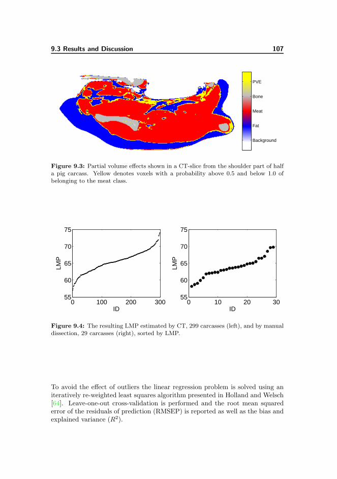
9.3 Results and Discussion 107

Background

Fat

Meat

Bone

PVE

Figure 9.3: Partial volume effects shown in a CT-slice from the shoulder part of halfa pig carcass. Yellow denotes voxels with a probability above 0.5 and below 1.0 ofbelonging to the meat class.

0 100 200 30055

60

65

70

75

LMP

ID0 10 20 30

55

60

65

70

75

LMP

ID

Figure 9.4: The resulting LMP estimated by CT, 299 carcasses (left), and by manualdissection, 29 carcasses (right), sorted by LMP.

To avoid the effect of outliers the linear regression problem is solved using aniteratively re-weighted least squares algorithm presented in Holland and Welsch[64]. Leave-one-out cross-validation is performed and the root mean squarederror of the residuals of prediction (RMSEP) is reported as well as the bias andexplained variance (R2).

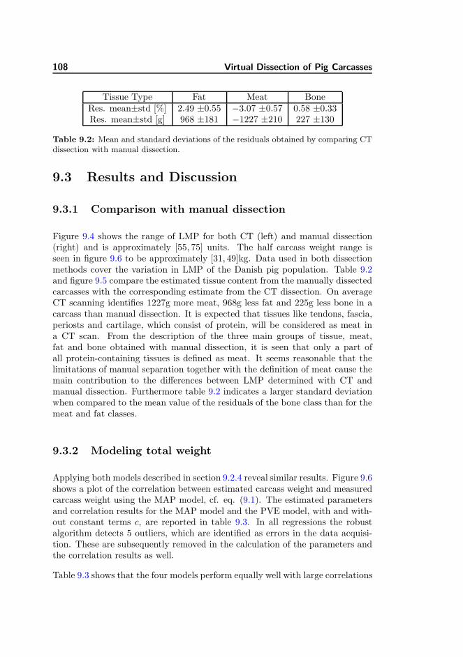
108 Virtual Dissection of Pig Carcasses

Tissue Type Fat Meat BoneRes. mean±std [%] 2.49 ±0.55 −3.07 ±0.57 0.58 ±0.33Res. mean±std [g] 968 ±181 −1227 ±210 227 ±130

Table 9.2: Mean and standard deviations of the residuals obtained by comparing CTdissection with manual dissection.

9.3 Results and Discussion

9.3.1 Comparison with manual dissection

Figure 9.4 shows the range of LMP for both CT (left) and manual dissection(right) and is approximately [55, 75] units. The half carcass weight range isseen in figure 9.6 to be approximately [31, 49]kg. Data used in both dissectionmethods cover the variation in LMP of the Danish pig population. Table 9.2and figure 9.5 compare the estimated tissue content from the manually dissectedcarcasses with the corresponding estimate from the CT dissection. On averageCT scanning identifies 1227g more meat, 968g less fat and 225g less bone in acarcass than manual dissection. It is expected that tissues like tendons, fascia,periosts and cartilage, which consist of protein, will be considered as meat ina CT scan. From the description of the three main groups of tissue, meat,fat and bone obtained with manual dissection, it is seen that only a part ofall protein-containing tissues is defined as meat. It seems reasonable that thelimitations of manual separation together with the definition of meat cause themain contribution to the differences between LMP determined with CT andmanual dissection. Furthermore table 9.2 indicates a larger standard deviationwhen compared to the mean value of the residuals of the bone class than for themeat and fat classes.

9.3.2 Modeling total weight

Applying both models described in section 9.2.4 reveal similar results. Figure 9.6shows a plot of the correlation between estimated carcass weight and measuredcarcass weight using the MAP model, cf. eq. (9.1). The estimated parametersand correlation results for the MAP model and the PVE model, with and with-out constant terms c, are reported in table 9.3. In all regressions the robustalgorithm detects 5 outliers, which are identified as errors in the data acquisi-tion. These are subsequently removed in the calculation of the parameters andthe correlation results as well.

Table 9.3 shows that the four models perform equally well with large correlations

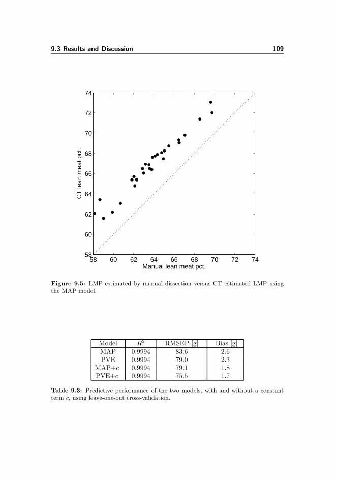
9.3 Results and Discussion 109

58 60 62 64 66 68 70 72 7458

60

62

64

66

68

70

72

74

CT

lean

mea

t pct

.

Manual lean meat pct.

Figure 9.5: LMP estimated by manual dissection versus CT estimated LMP usingthe MAP model.

Model R2 RMSEP [g] Bias [g]MAP 0.9994 83.6 2.6PVE 0.9994 79.0 2.3

MAP+c 0.9994 79.1 1.8PVE+c 0.9994 75.5 1.7

Table 9.3: Predictive performance of the two models, with and without a constantterm c, using leave-one-out cross-validation.

110 Virtual Dissection of Pig Carcasses

30 35 40 45 5030

35

40

45

50

Weight [kg]

Est

imat

ed w

eigh

t [kg

]

Figure 9.6: Estimated weight using the MAP model versus measured weight.

9.3 Results and Discussion 111

MAP PVE MAP+c PVE+c0.98

0.99

1

1.01

ρf

[kg/

dm3 ]

MAP PVE MAP+c PVE+c1.1

1.11

1.12

ρm

[kg/

dm3 ]

MAP PVE MAP+c PVE+c

1.3

1.4

1.5

1.6

ρb

[kg/

dm3 ]

MAP+c PVE+c0

0.2

0.4

0.6

0.8c

[kg]

Figure 9.7: Estimated parameters and their corresponding 95% confidence intervalsfor the two models, with and without a constant term c.

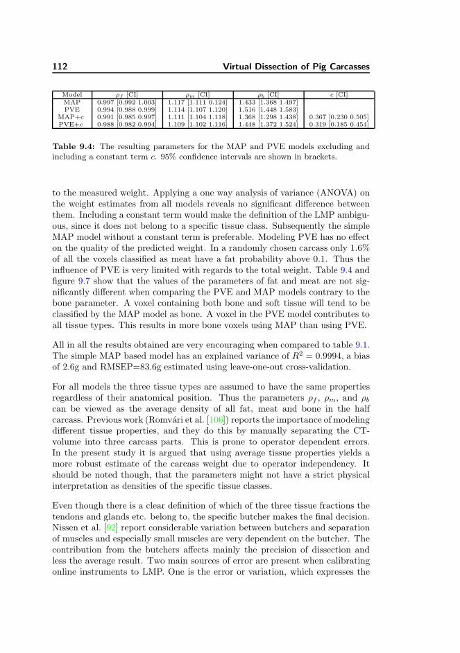
112 Virtual Dissection of Pig Carcasses

Model ρf [CI] ρm [CI] ρb [CI] c [CI]MAP 0.997 [0.992 1.003] 1.117 [1.111 0.124] 1.433 [1.368 1.497]PVE 0.994 [0.988 0.999] 1.114 [1.107 1.120] 1.516 [1.448 1.583]

MAP+c 0.991 [0.985 0.997] 1.111 [1.104 1.118] 1.368 [1.298 1.438] 0.367 [0.230 0.505]PVE+c 0.988 [0.982 0.994] 1.109 [1.102 1.116] 1.448 [1.372 1.524] 0.319 [0.185 0.454]

Table 9.4: The resulting parameters for the MAP and PVE models excluding andincluding a constant term c. 95% confidence intervals are shown in brackets.

to the measured weight. Applying a one way analysis of variance (ANOVA) onthe weight estimates from all models reveals no significant difference betweenthem. Including a constant term would make the definition of the LMP ambigu-ous, since it does not belong to a specific tissue class. Subsequently the simpleMAP model without a constant term is preferable. Modeling PVE has no effecton the quality of the predicted weight. In a randomly chosen carcass only 1.6%of all the voxels classified as meat have a fat probability above 0.1. Thus theinfluence of PVE is very limited with regards to the total weight. Table 9.4 andfigure 9.7 show that the values of the parameters of fat and meat are not sig-nificantly different when comparing the PVE and MAP models contrary to thebone parameter. A voxel containing both bone and soft tissue will tend to beclassified by the MAP model as bone. A voxel in the PVE model contributes toall tissue types. This results in more bone voxels using MAP than using PVE.

All in all the results obtained are very encouraging when compared to table 9.1.The simple MAP based model has an explained variance of R2 = 0.9994, a biasof 2.6g and RMSEP=83.6g estimated using leave-one-out cross-validation.

For all models the three tissue types are assumed to have the same propertiesregardless of their anatomical position. Thus the parameters ρf , ρm, and ρbcan be viewed as the average density of all fat, meat and bone in the halfcarcass. Previous work (Romvari et al. [106]) reports the importance of modelingdifferent tissue properties, and they do this by manually separating the CT-volume into three carcass parts. This is prone to operator dependent errors.In the present study it is argued that using average tissue properties yields amore robust estimate of the carcass weight due to operator independency. Itshould be noted though, that the parameters might not have a strict physicalinterpretation as densities of the specific tissue classes.

Even though there is a clear definition of which of the three tissue fractions thetendons and glands etc. belong to, the specific butcher makes the final decision.Nissen et al. [92] report considerable variation between butchers and separationof muscles and especially small muscles are very dependent on the butcher. Thecontribution from the butchers affects mainly the precision of dissection andless the average result. Two main sources of error are present when calibratingonline instruments to LMP. One is the error or variation, which expresses the

9.4 Conclusions 113

imperfect relation between the reference LMP and the online measurements,including the accuracy of the online measurements, and the other one is theaccuracy of the dependent variable i.e. the reference LMP.

LMP based on CT is a very promising candidate for an instrumental referencefor pig carcass classification. Previous investigations have shown very high re-peatability. However, before CT LMP can be used as a global reference, ithas to be documented that the results can be reproduced independently of CTinstruments, time and pig population. The method described in this paper isbased on a specific scanning protocol and reconstruction algorithm. Althoughthe method seems robust to these factors a thorough documentation will benecessary. Especially the choice of slice thickness, resolution and reconstructionalgorithm has to be general and available on all types and makes of CT scanners.A possible tool to ensure the reproducibility over time, including a possible biascorrection, could be calibration using phantoms that mimic different types ofcarcasses with known values of LMP. How such phantoms should be designed isan area of future research.

Replacing the manually determined LMP with CT based LMP will improve thecalibration problem significantly, even though the lack of a perfect relationshipis an important issue. Disregarding the fixed costs related to the purchaseof a CT scanner and installing it in a trailer, the lower costs using CT is aconsiderable advantage compared to manual dissection. If only the maintenanceof the scanner is taken into account alongside the salary of the operators, a CTbased LMP costs less than half that of a manual dissection.

9.4 Conclusions

Previous work shows CT-based methods as robust compared to manual dissec-tion, and as such constitute a suitable reference. This work presents a robustand accurate calibration reference, where variation due to manual interventionis minimized. Given a model of the carcass weight, the LMP can be estimatedbased on the classification of the volume elements (voxels) in the CT volume.Using this more accurate method as a reference will make the calibration pro-cedures of other LMP sensors much more standardized and accurate.

Contextual models based on segmentation of the carcass into three classes isvalidated on a large data set of 299 half pig carcasses. Incorporating the influenceof partial volume effects is found not to be significantly better than a maximum-a-posteriori model. All models correlate very well with the full weight of the halfcarcasses, with the simple maximum-a-posteriori based model being the modelof choice. The model has an explained variance of R2 = 0.9994, a bias of 2.6g

114 Virtual Dissection of Pig Carcasses

and a root-mean-squared error of prediction of RMSEP=83.6g. These resultsare very encouraging compared to previous work, for which reason the methodis suggested as a new reference for calibration of sensors used for pig carcassgrading.

Acknowledgements

The CT data was provided by the Danish Meat Research Institute as a part ofthe project ”The Virtual Slaughterhouse” funded by the Danish Pig Levy Fundand the Directorate for Food, Fisheries and Agri Business.

Chapter 10

Accelerated 3D Image

Registration

Martin Vester-Christensen, Søren G. Erbou, Sune Darkner and Rasmus

Larsen

Abstract

Image registration is an important task in most medical imaging appli-cations. Numerous algorithms have been proposed and some are widelyused. However, due to the vast amount of data collected by eg. a com-puted tomography (CT) scanner, most registration algorithms are very slowand memory consuming. This is a huge problem especially in atlas build-ing, where potentially hundreds of registrations are performed. This paperdescribes an approach for accelerated image registration. A grid-basedwarp function proposed by Cootes and Twining, parameterized by the dis-placement of the grid-nodes, is used. Using a coarse-to-fine approach, thecomposition of small diffeomorphic warps, results in a final diffeomorphicwarp. Normally the registration is done using a standard gradient-basedoptimizer, but to obtain a fast algorithm the optimization is formulatedin the inverse compositional framework proposed by Baker and Matthews.By switching the roles of the target and the input volume, the Jacobianand the Hessian can be pre-calculated resulting in a very efficient optimiza-tion algorithm. By exploiting the local nature of the grid-based warp, thestorage requirements of the Jacobian and the Hessian can be minimized.Furthermore, it is shown that additional constraints on the registration,such as the location of markers, are easily embedded in the optimization.The method is applied on volumes built from CT-scans of pig-carcasses, andresults show a two-fold increase in speed using the inverse compositionalapproach versus the traditional gradient-based method.

116 Accelerated 3D Image Registration

10.1 Introduction

Registration of images is an important an actively researched area of medicalimaging. It is the task of transforming the geometry of two or more imagessuch that their corresponding regions are aligned. The need may arise fromcomparison of images from different imaging modalities, from images obtainedat different times, from different patients, or from comparison with a patientatlas. Registration is needed in a wide variety of medical applications, eg. fordiagnostic purposes, for pre-surgery planning or for treatment estimation. Themedical imaging hardware of today produce images of high resolution, and asa consequence a huge amount of data need processing in order to solve theregistration problem. The requirements on the processing hardware are veryhigh in terms of storage capability, CPU speed, and maybe most importantlyin memory capacity.

A range of different registration algorithms have been produced in the recentyears. The algorithm described in this paper, belongs to the class of parameter-ized methods. Hence the registration can be described by a set of parameters.Existing methods includes Rueckert [108] et al. using B-splines on a grid todefine the warp-field, Cootes [30] et al uses bounded diffeomorphisms, warp-ing pixels inside a unit sphere based on the displacement of the sphere center.An example of the non-parametric approach is found in Christensen [22] et al.which solve partial differential equations for fluid motions to align images.

This paper presents the acceleration of an image registration algorithm [31] byCootes et al.. An inverse compositional [7] optimization scheme, proposed byBaker and Matthews, is used. It is a Gauss-Newton approach, but in whichthe Jacobian and the estimated Hessian can be precomputed. However, tobe tractable memory wise, this requires exploitation of the properties of theregistration algorithm. An additional benefit of the Gauss-Newton approach isthe ease of which addition of soft constraints on the registration can be added.Comparison is made with optimization using the Lucas-Kanade scheme.

The paper consist of the following. First the registration algorithm is described.In 10.2.1 the image registration algorithm is described, followed by outlining ofthe Lucas-Kanade algorithm, in 10.2.2, and the inverse compositional optimiza-tion algorithm, in 10.2.3. Addition of soft constraints is described in 10.2.4.Section 10.3 describes the results obtained by comparing the two optimizationschemes.

10.2 Methods 117

10.2 Methods

The image registration algorithm utilized in this paper is proposed by Cootes [31]et al. which builds on the algorithms presented by Rueckert [109] et al. The im-age registration is performed by composing a series of grid-based diffeomorphicwarps which ensures the resulting warp being diffeomorphic.

10.2.1 Grid-Based Diffeomorphisms

A grid-based warp is represented by a grid of nodes1, see figure 10.1. The trans-formation W of a pixel x = (x, y, z) is found by interpolating the displacementd of its surrounding grid nodes. In 3D the interpolating scheme is as below,

W(x;α) = k(x− i)k(y − j)k(z − l)di,j,l (10.1)

+ k(i+ 1− x)k(y − j)k(z − l)di+1,j,l

+ k(x− i)k(j + 1− y)k(z − l)di,j+1,l

+ k(i+ 1− x)k(j + 1− y)k(z − l)di+1,j+1,l

+ k(x− i)k(y − j)k(l + 1− z)di,j,l+1

+ k(i+ 1− x)k(y − j)k(l + 1− z)di+1,j,l+1

+ k(x− i)k(j + 1− y)k(l + 1− z)di,j+1,l+1

+ k(i+ 1− x)k(j + 1− y)k(l + 1− z)di+1,j+1,l+1,

where k() denotes a suitable kernel function which is non-zero only for i ≤ x <i + 1, j ≤ y < j + 1 and l ≤ z < l + 1. The warp is parameterized with thecomponents of the displacement vectors d. Thus, with a 3×3×3 grid in 3D, thewarp consist of 81 parameters. The kernel is chosen as k(r) = 1

2 (1 + cos(πr))which gives a smooth and invertible mapping [31] given that − 1

π< r < 1

π.

Using the interpolating scheme the warp is regularized by the coarseness ofthe grid. Thus, a pixel cannot move outside the bounding box provided by thesurrounding grid nodes. However, to represent a complex transformation severalsimple warps can be composed,

W(x;p) = W(x; δ1) ◦W(x; δ2) . . .W(x; δn−1) ◦W(x; δn), (10.2)

where W(x; δ1) ◦W(x; δ2) = W(W(x; δ2); δ1) denotes the composition of twowarps. The warps are applied in a fine to coarse manner.

1The following is an elaboration on the paper [31] by Cootes et al, but is included here forcompleteness.

118 Accelerated 3D Image Registration

(a) Before.

(b) After.

Figure 10.1: The displacement of a pixel is governed by the displacement of itssurrounding grid nodes [116].

10.2 Methods 119

10.2.2 Image Registration using the Lucas-Kanade Algo-

rithm

The goal of the image registration algorithm is to align a target and a input im-age such that the difference is minimized. This is quantified by the minimizationof the sum of squared residuals,

F(p) =∑

x

[T (x)− I(W(x;p))]2, (10.3)

where I is the input image and T is the target image. This can be minimizedusing a Gauss-Newton optimization scheme [82],

F (p) =1

2

∑

x

[T (x)− I(W(x;p+∆p))]2, (10.4)

which by Taylor expansion and solving for ∆p gives,

∆p = H−1∑

x

[

∇I(W(x;p))∂W(x;p)

∂p

]⊤

E(x), (10.5)

where H is the Gauss-Newton approximation to the Hessian,

H =∑

x

[

∇I(W(x;p))∂W(x;p)

∂p

]⊤ [

∇I(W(x;p))∂W(x;p)

∂p

]

, (10.6)

and the error is,E(x) = T (x)− I(W(x;p)). (10.7)

The warp parameters p are updated using,

p← p+∆p. (10.8)

The Jacobian is found to be,

J =∑

x

[

∇I(W(x;p))∂W(x;p)

∂p

]

, (10.9)

where ∇I(W(x;p)) is the image gradient of the input image sampled at the

points W(x;p), and ∂W(x;p)∂p

is the derivative of the warp function with respectto the parameters.

This optimization scheme requires computation of the Jacobian J and the in-verse Hessian H−1 at each iteration. For large volumes and large grids, this isvery computationally demanding. However, the Hessian is symmetric and verysparse thus enabling the utilization of fast schemes for solving large sparse linearequations [47].

120 Accelerated 3D Image Registration

10.2.3 Inverse Compositional Image Registration

To overcome the drawbacks of the Gauss-Newton scheme of calculating theJacobian and the Hessian in each iteration, Baker and Matthews [7] recentlyproposed the Inverse Compositional Algorithm, in which the Jacobian and theHessian can be precomputed. As the name implies the algorithm consists of twoinnovations. The compositional part refers to the updating of the parametersand the inverse part indicates that the image and the target switches roles. Thecost function in 10.4 is changed to,

Fic(p) =1

2

∑

x

[T (W(x; ∆p)) − I(W(x;p))]2. (10.10)

Solving for ∆p gives,

∆p = −H−1ic

∑

x

[

∇T (x)∂W(x;0)

∂p

]⊤

E(x). (10.11)

The update to the warp is,

W(x;p) = W(x;p) ◦W(x; ∆p)−1, (10.12)

In equation 10.10 it can be seen that the incremental warp W(x; ∆p) appliesonly to the target T , and thus the Taylor expansion is around p = 0, yieldingthe Jacobian

Jic =∑

x

[

∇T (W(x;0))∂W(x;0)

∂p

]

. (10.13)

and thus the Hessian Hic is,

Hic =∑

x

[

∇T (x)∂W(x;0)

∂p

]⊤ [

∇T (x)∂W(x;0)

∂p

]

. (10.14)

The Jacobian is independent of p and ∇T (x) is the image gradient of the target,thus enabling precomputation of the Jacobian and the Hessian.

Baker and Matthews [7] proves that the update ∆p calculated using the inversecompositional algorithm is equivalent, to a first order approximation, to theupdate calculated using the Lucas-Kanade algorithm.

10.2.4 Adding Constraints

Baker et al. [8] describe how to incorporate prior information on the warp pa-rameters. This could for instance be landmark or volume constraints formulated

10.2 Methods 121

as an additional term in the expression to be minimized, i.e. as weighted softconstraints to equation 10.3,

1

2

∑

x

[T (x)− I(W(x;p))]2 + α

K∑

i=1

C2i (p). (10.15)

K is the number of constraints, Ci is a vector of functions containing the prior onthe parameters for the ith constraint and α is a weight controlling the emphasison the prior term. In the inverse compositional framework this corresponds toequation 10.10,

1

2

∑

x

[T (W(x; ∆p)− I(W(x;p))]2 + α

K∑

i=1

C2i (p+

∂p′

∂∆p∆p). (10.16)

Approximating this with a first order Taylor expansion gives the following up-date equations for the gradient ∆p and the Hessian,

∆p = −H−1ic,Ci

[

∑

x

[

∇T (x)∂W(x;0)

∂p

]⊤

E(x) (10.17)

+ αGr

K∑

i=1

[

∂Ci

∂p

∂p′

∂∆p

]T

Ci(p)

]

Hic,Ci= Hic + αHe

K∑

i=1

[

∂Ci

∂p

∂p′

∂∆p

]T [

∂Ci

∂p

∂p′

∂∆p

]

. (10.18)

The computational cost of adding priors is that the Hessian is not constantanymore. The costs is O(nN + n2K + n3) compared to O(nN + n2) withoutpriors. As long as the number of constraints and the number of parameters aresmaller than the number of pixels/voxels (K << N and n << N), this cost isnegligible. In order to make the prior terms robust to the number of constraints,the α weights are chosen relative to the L2-norm of the term without priors,

αGr = αRel

∥

∥

∥

∑

x

[

∇T (x)∂W(x;0)∂p

]T

E(x)∥

∥

∥

L2∥

∥

∥

∑Ki=1

[

∂Ci

∂p∂p′

∂∆p

]T

Ci(p)∥

∥

∥

L2

(10.19)

αHe = αRel

∥

∥

∥Hic

∥

∥

∥

L2∥

∥

∥

∑Ki=1

[

∂Ci

∂p∂p′

∂∆p

]T [

∂Ci

∂p∂p′

∂∆p

] ∥

∥

∥

L2

, (10.20)

where αRel >= 0 is the relative weighting between the two terms. αRel = 0corresponds to the inverse compositional without the prior term.

122 Accelerated 3D Image Registration

10.2.5 Fast Grid-Based Image Registration

The inverse compositional scheme described above requires the computationthe Jacobian from equation 10.13 and subsequently the Hessian from equation10.14. To take full advantage of the inverse compositional method, they mustbe precalculated and stored. However, the storage requirement of the Jacobiancan be very large. In a naive implementation using a simple 3 × 3 × 3 grid,space is needed for 81 · N floating point numbers with N being the number ofpixels in the image and potentially very large. So great care must be taken inthe implementation in order to exploit the speed gain provided by the inversecompositional framework.

10.2.5.1 Calculating the Jacobian and the Hessian

The Jacobian consist of the gradient ∇T (x) =[

∂T∂x

∂T∂y

∂T∂z

]

of the target

image and the derivative of the warp ∂W∂p

. ∇T (x) can be found using a simplefinite difference method or more elaborate methods using B -splines or similarinterpolating methods. The warp derivatives are very simple to calculate. Asmentioned, the parameters of the warp are simply the 3 ·mnp ordinates of thedisplacements of the nodes,

p =[

dx1,1,1 dy1,1,1 dz1,1,1 dx2,1,1 dy2,1,1 dz2,1,1 . . . dxm,n,p dym,n,p dzm,n,p

]

, (10.21)

for a m× n× p grid. This and equation 10.1 yields

∂W

∂dxi,j,l=

∂W

∂dyi,j,l=

∂W

∂dzi,j,l, (10.22)

meaning that the derivatives corresponding to the x, y, z components of one dis-placement vector are equal. Each pixel x contributes to eight partial derivativesonly, corresponding to the eight surrounding grid nodes, cf. figure 10.2 for a 2Dexample. Thus, for N pixels, an N×8 floating point value representation of ∂W

∂p

is possible using a simple lookup method. However, since the kernel functionk() only operates on the distance from a contributing pixel x to a node, an evensparser representation of only Nreg × 8 is possible. Nreg is the number of pixelssurrounded by 8 neighboring grid nodes. For increasing grid sizes the spacerequirement goes down.

Another property of ∂W∂p

is seen from,

k(i+ 1− x) = 1− k(x− i), (10.23)

which holds for y and z as well. For a neighborhood of grid nodes, the derivative

10.2 Methods 123

Figure 10.2: The derivative of the warp with respect to the node in the lower leftcorner. It is non-zero only in the region bounded by the neighboring nodes.

124 Accelerated 3D Image Registration

at x = (x, y, z) wrt. the parameters of the warp has the form,

∂W

∂pi,j,l= k(x− i)k(y − j)k(z − l)

∂W

∂pi+1,j,l= (1− k(x − i))k(y − j)k(z − l)

...∂W

∂pi+1,j+1,l+1= (1− k(x − i))(1− k(y − j))(1 − k(z − l)) (10.24)

Thus, to evaluate the derivative contribution for a single pixel x, only threekernel function evaluations, k(x − i), k(y − j) and k(z − l) are needed. Thederivatives can then be found using simple multiplications and subtractions.

Finally the Jacobian is calculated as in equation 10.13, which means multiplyingthe warp derivatives with the image gradients. However, the Jacobian with thesparse representation mentioned above has a size of N ×24 floating point valueswhich requires a large amount of memory. Subsequently a compromise has tobe made, and in this work the image gradients and the warp derivatives arestored separately, yielding space requirement for N × 3 plus Nreg × 8 numbers.This means the multiplication of the gradients and the derivatives must beperformed each time the Jacobian is needed, yet precalculation of the Hessianis still possible.

The Hessian is calculated as in equation 10.14. The sparseness of the Jacobianis transferred into the Hessian. Figure 10.3 depicts the sparseness of the Hessianfor three grid sizes. Solving equation 10.11 requires the inversion of the Hes-sian matrix. This usually destroys the sparseness and is very computationallydemanding. Furthermore, the Hessian can be very ill-conditioned, but makinguse of iterative methods [47] for solving sparse linear equations, the inversion ofthe Hessian can be avoided.

10.2.5.2 The Image Registration Algorithm

To estimate the transformation of the input image I into the target image Tminimization of equation 10.10 with respect to p is required. This is done byfirst applying a coarse grid, eg. 3× 3× 3, and iteratively solving equation 10.11until convergence. Subsequently a finer grid, eg. 5 × 5 × 5, is applied, andso forth. This enables the estimation of small local transformations while stillbeing diffeomorphic [31]. A multilevel approach, using downsampled versions ofthe images, is adopted to avoid local minima. Consequently, for each grid size,optimization is done in a coarse-to-fine manner as well, starting the optimization

10.2 Methods 125

0 10 20 30 40 50 60 70 80

0

10

20

30

40

50

60

70

80

nz = 3087

(a) 81× 81 matrix.

0 50 100 150 200 250 300 350

0

50

100

150

200

250

300

350

nz = 14052

(b) 375× 375 matrix.

0 200 400 600 800 1000 1200 1400 1600 1800 2000

0

200

400

600

800

1000

1200

1400

1600

1800

2000

nz = 49791

(c) 2187 × 2187 matrix.

Figure 10.3: Plot of non-zero elements in Hessian matrices, for grid sizes of 3×3×3,5× 5× 5 and 9× 9× 9 .

126 Accelerated 3D Image Registration

on a finer downsampling level with the parameters estimated on a coarser level.See figure 10.4. At each iteration equation 10.12 must be used to update theparameters. In this work the parameters of W(x;∆p) is estimated with thefirst order approximation [8] −∆p. Thus the parameter update from equation10.12 has the form,

p← p−∆p. (10.25)

When the optimization for one grid size converges, a finer grid is applied, ie.a 3 × 3 × 3 is replaced with a 5 × 5 × 5. Composition of warps of differencegrid sizes is done in a simple manner. Figure 10.5 depicts the scheme. The gridnodes of the higher level warp are transformed with the lower level warp. Thus,the parameters from the lower level are transported into the higher level warp.

10.3 Results

10.3.1 3D Non-Rigid Registration

5 CT-volumes of the hind part of porcine carcasses are cross-registered to com-pare the inverse compositional algorithm with the Lucas-Kanade algorithm. Thevolumes are approximately 512x512x170 voxels of size [0.67,0.67,2] mm. Afterrigid registration the two algorithms for non-rigid registration are applied andthe speed and accuracy are compared. Due to time considerations the 20 regis-trations are done with images downsampled to 1

16 ,18 and 1

4 of the original imagesize for grids of size [3,5,7,9] per dimension. Figure 10.6 shows three slice planesof a volume and their corresponding error images after a typical registration.The main errors are along the border of the volume due to the large differencein value between background and volume.

Rows 1 and 2 in table 10.1 show the mean value and standard deviation of thenumber of iterations used before convergence, the final registration error andthe time consumption for the two algorithms. Row 3 shows the mean improve-ment when using the IC algorithm and row 4 shows a paired T-test of significantdifferences in the mean values. There are highly significant improvements (de-noted by 1) in both speed and number of iterations. The mean final registrationerror of the two methods are not significantly different. In this simple testit therefore shows that the inverse compositional algorithm is as accurate asthe Lucas-Kanade algorithm, as expected, but is twice as fast for registrationof CT-volumes. The results are obtained using a Dell Latitude 810D, with a2.0Ghz CPU and 2 gb of ram. The implementation of the Lucas-Kanade al-gorithm utilizes the same sparseness properties as the implementation of theinverse compositional algorithm. Thus, the algorithms perform similar memorywise. The speed increase of the inverse compositional algorithm is due to the

10.3 Results 127

(a) Coarser level.

(b) Finer level.

Figure 10.4: Plot of the warpfield estimated on a coarse image level and the corre-sponding field in a finer level.

Table 10.1: Comparison between the Lucas-Kanade algorithm and the inverse com-positional algorithm based on 20 registrations.

Iterations Final Error Speed [sec.]Lucas-Kanade (mean±std.) 160± 29 (7.6± 4.1) · 1011 436± 128Inverse Compositional (mean±std.) 140± 15 (7.5± 4.0) · 1011 222 ± 45Mean improvement with IC (%) 13 2 49Paired T-test for difference in mean,1=mean values are sign. diff. 1 (p < 0.006) 0 1 (p < 10−3)

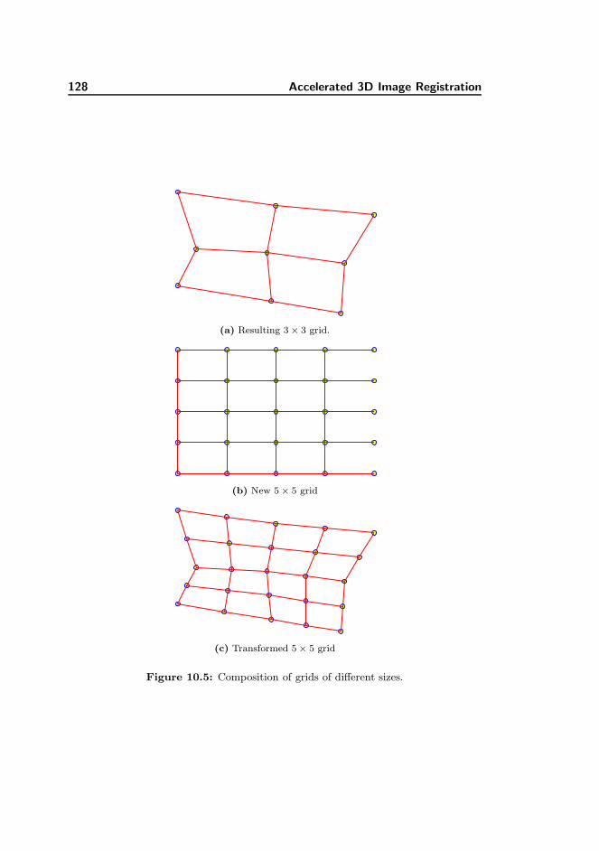
128 Accelerated 3D Image Registration

(a) Resulting 3× 3 grid.

(b) New 5× 5 grid

(c) Transformed 5× 5 grid

Figure 10.5: Composition of grids of different sizes.

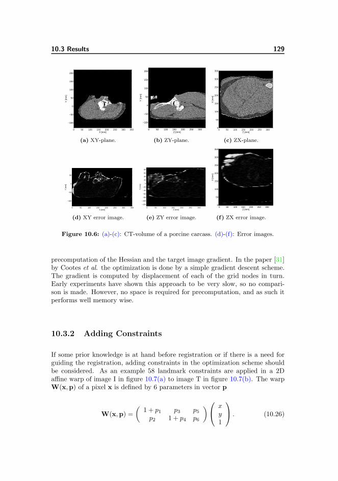
10.3 Results 129

X [mm]

Y [m

m]

0 50 100 150 200 250 300 350

−100

−50

0

50

100

150

200

(a) XY-plane.

Z [mm]

Y [m

m]

0 50 100 150 200 250 300

−100

−50

0

50

100

150

200

(b) ZY-plane.

Z [mm]

X [m

m]

0 50 100 150 200 250 3000

50

100

150

200

250

300

350

(c) ZX-plane.

X [mm]

Y [m

m]

0 50 100 150 200 250 300 350

−100

−50

0

50

(d) XY error image.

Z [mm]

Y [m

m]

0 50 100 150 200 250 300

−120

−100

−80

−60

−40

−20

0

20

40

60

80

(e) ZY error image.

Z [mm]X

[mm

]

0 50 100 150 200 250 3000

50

100

150

200

250

300

350

(f) ZX error image.

Figure 10.6: (a)-(c): CT-volume of a porcine carcass. (d)-(f): Error images.

precomputation of the Hessian and the target image gradient. In the paper [31]by Cootes et al. the optimization is done by a simple gradient descent scheme.The gradient is computed by displacement of each of the grid nodes in turn.Early experiments have shown this approach to be very slow, so no compari-son is made. However, no space is required for precomputation, and as such itperforms well memory wise.

10.3.2 Adding Constraints

If some prior knowledge is at hand before registration or if there is a need forguiding the registration, adding constraints in the optimization scheme shouldbe considered. As an example 58 landmark constraints are applied in a 2Daffine warp of image I in figure 10.7(a) to image T in figure 10.7(b). The warpW(x,p) of a pixel x is defined by 6 parameters in vector p

W(x,p) =

(

1 + p1 p3 p5p2 1 + p4 p6

)

xy1

. (10.26)

130 Accelerated 3D Image Registration

The first order term in the linearization of the additive update is

∂p′

∂∆p= −

1 + p1 p3 0 0 0 0p2 1 + p4 0 0 0 00 0 1 + p1 p3 0 00 0 p2 1 + p4 0 00 0 0 0 1 + p1 p30 0 0 0 p2 1 + p4

. (10.27)

The error function of the prior part is defined as

Ci = (LmT,i −W(LmI,i;p)), (10.28)

where LmT,i is the ith landmark in the target image T and LmI,i is the ith

landmark in the input image I. The Jacobian of Ci then is

∂Ci

∂p= −

(

LmI,i,x 0 LmI,i,y 0 1 00 LmI,i,x 0 LmI,i,y 0 1

)

, (10.29)

where LmI,i,x and LmI,i,y are the x- and y-coordinates, respectively, of the ith

landmark in I.

Figure 10.7(c) shows the L2-norm of the intensity and prior error as αRel isincreased. αRel=0 corresponds to no constraints and αRel=1 corresponds to theintensity and the constraints being weighted equally. The constraints improvethe registration as long as the intensity error is decreasing, i.e. for α-valuesapproximately between 0.8 and 1.6. The prior error will off course decreasewith increasing α-value. How much weight to put on the constraints dependson the application but for this example weighting intensity and prior more or lessequal gives the best result. Figures 10.8(a)-10.8(c) show the difference betweenthe input image I and the target image T warped into the coordinate frameof I, for αRel=0,1 and 2. The improvement in registration without constraintscompared to the registration with the intensity and constraints weighted equallyis obvious, especially in the area around the jaw.

Applying similar constraints as described in section 10.2.4 to the nonrigid caseor in 3D is straightforward, all you need to do is to define Ci and compute theJacobian and ∂p′/∂∆p.

10.4 Conclusion

This paper has presented an algorithm for registration of 3D images. Regis-tration is done using grid-based warps in a coarse-to-fine manner, enabling the

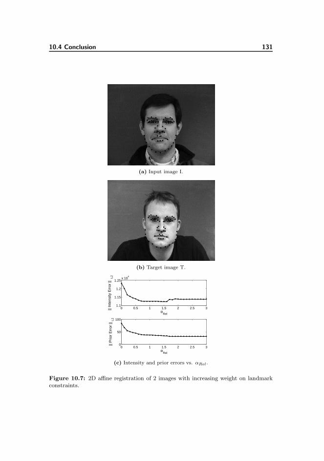
10.4 Conclusion 131

(a) Input image I.

(b) Target image T.

0 0.5 1 1.5 2 2.5 31.1

1.15

1.2

1.25x 10

4

αRel

|| In

tens

ity E

rror

|| L2

0 0.5 1 1.5 2 2.5 30

50

100

αRel

|| P

rior

Err

or ||

L2

(c) Intensity and prior errors vs. αRel.

Figure 10.7: 2D affine registration of 2 images with increasing weight on landmarkconstraints.

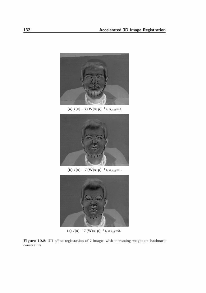
132 Accelerated 3D Image Registration

(a) I(x) − T (W(x;p)−1), αRel=0.

(b) I(x)− T (W(x;p)−1), αRel=1.

(c) I(x)− T (W(x;p)−1), αRel=2.

Figure 10.8: 2D affine registration of 2 images with increasing weight on landmarkconstraints.

10.4 Conclusion 133

registration of even fine structures in the images while still being diffeomorphic.Using the inverse compositional framework for optimization, the algorithm per-forms very fast. Exploitation of the sparseness of the grid-based warps and theproperties of the interpolating kernel, enables the precomputation of the Hes-sian and the target image gradient. The algorithm has a two-fold increase inspeed compared to a Lucas-Kanade based algorithm.

Acknowledgments

The 2D images are part of the DTU Face Database [116] and the CT data wasprovided by the Danish Meat Research Institute as a part of the project ”TheVirtual Butcher” funded by the Danish Pig Levy Fund and the Directoratefor Food, Fisheries and Agri Business. The authors would also like to thankthe IMM ITMAN graduate school at the Technical University of Denmark forsupport.

134 Accelerated 3D Image Registration

Appendix A

Demos

This appendix contain examples of two demo-tools produced during the courseof the project. Both where implemented in order to demonstrate the conceptsbehind the Virtual Slaughterhouse to employees in the Danish slaughterhouseindustry.

A.1 OinkExplorer

Live demonstration of the concept of virtual cuts. A tool for interactive place-ment of a cutting plane. Real time estimated of the weight of each product isdisplayed while the plane is moved.

136 Demos

Figure A.1: Demo application: OinkExplorer. Demonstrating interactive placementof a cutting plane.

A.2 OinkDemo 137

Figure A.2: Demo application: OinkDemo. Cuts a middle part into of a carcass intoribs, 18cm back and belly.

A.2 OinkDemo

Demonstration of automatic cutting of a middle part of a carcass into ribs, 18cmback and belly. Fat, meat and bone content is displayed.

138 Demos

List of Tables

7.1 The average landmark and intensity variance for six levels of regularization. . . 81

7.2 Parameters of the yield prediction models for the loin and 18cm back products. 81

7.3 Parameters of the yield prediction models for the loin and 18cm back productsusing only the lean meat as predictor. . . . . . . . . . . . . . . . . . . . . . . . 82

8.1 An overview of the applied scanning protocols. First protocol (No. 1) is arbi-trarily used as reference. . . . . . . . . . . . . . . . . . . . . . . . . . . . . . . . 95

8.2 Weight estimation. . . . . . . . . . . . . . . . . . . . . . . . . . . . . . . . . . . 97

8.3 LMPCT estimation. . . . . . . . . . . . . . . . . . . . . . . . . . . . . . . . . . 97

9.1 Previous work. Papers [34], [25], [106] and [68] apply PLS-methods on his-tograms for meat pixels, modeling the lean meat weight obtained from dis-section. [84] apply a contextual Bayesian classifier and linear regression forpredicting the full weight of half carcasses. R2 is the explained variance, RM-SEP/C are the rms errors of prediction/calibration, with the corresponding biasreported in some cases. . . . . . . . . . . . . . . . . . . . . . . . . . . . . . . . . 104

9.2 Mean and standard deviations of the residuals obtained by comparing CT dis-section with manual dissection. . . . . . . . . . . . . . . . . . . . . . . . . . . . 108

9.3 Predictive performance of the two models, with and without a constant termc, using leave-one-out cross-validation. . . . . . . . . . . . . . . . . . . . . . . . 109

9.4 The resulting parameters for the MAP and PVE models excluding and includinga constant term c. 95% confidence intervals are shown in brackets. . . . . . . . 112

140 LIST OF TABLES

10.1 Comparison between the Lucas-Kanade algorithm and the inverse composi-tional algorithm based on 20 registrations. . . . . . . . . . . . . . . . . . . . . . 127

List of Figures

2.1 Examples of automation in a Danish slaughterhouse. Carcasses hanging on barsin the equalization room(top left). Top right and lower left images depicts beforeand after a split into three parts. The lower right image depicts a slaughterrobot splitting the middle part into loin and belly. Images are courtesy ofDanish Meat Association. . . . . . . . . . . . . . . . . . . . . . . . . . . . . . . 8

2.2 Graphical rendering of the product flow in a slaughterhouse. The pigs enter insection A which is the killing zone, where they are stunned, killed by stickingand debled. They continue onto the slaughterline in section B where the carcassis split in halves and intestines, heart etc. are removed. Section C is the cuttingline in which the carcasses are cut into products. . . . . . . . . . . . . . . . . . 9

3.1 A back-splitting robot seen from the front. Courtesy of Danish Meat Association. 17

3.2 A half carcass prepared and ready for scanning. Courtesy of Danish MeatAssociation. . . . . . . . . . . . . . . . . . . . . . . . . . . . . . . . . . . . . . . 18

3.3 A carcass wrapped in low density plastic about to be scanned. Courtesy ofDanish Meat Association. . . . . . . . . . . . . . . . . . . . . . . . . . . . . . . 18

3.4 The principle of Computed Tomography. . . . . . . . . . . . . . . . . . . . . . 19

3.5 Histogram of voxels values in a typical pig, clamped in the range [−150; 150].The left peak corresponds to fat, the right peak to meat. Bone is found as thetail in the right side of the histogram. . . . . . . . . . . . . . . . . . . . . . . . 19

3.6 An axial slice of the carcass volume located in the middle part. . . . . . . . . . 20

3.7 A montage view of every second slice in a CT volume of a carcass. . . . . . . . 21

3.8 Sagittal and coronal views of a carcass. . . . . . . . . . . . . . . . . . . . . . . . 22

142 LIST OF FIGURES

3.9 Volumetric visualization of a half carcass using orthogonal slice planes. . . . . 22

3.10 X-Ray view of a carcass with landmarks overlain. . . . . . . . . . . . . . . . . . 23

3.11 Annotation scheme for the twelve most posterior ribs and the scapula. . . . . . 24

5.1 Images with different voxel dimensions. . . . . . . . . . . . . . . . . . . . . . . 33

5.2 Example of an image transformation turning a square into a circle. The topleft figure depicts the grid X overlaid with the displacement vectors. Top leftis the resulting grid Y . In the bottom row is shown the image before T (X)(left) and after T (Y ) (right) the transformation. . . . . . . . . . . . . . . . . . 35

5.3 A transformation of a rectangle. Top left is the starting rectangle with thegrid x overlain. Top right is the resulting circle sampled using the grid y. Thebottom figure depicts the resulting grid y. . . . . . . . . . . . . . . . . . . . . . 37

5.4 Affine transformation of a square. The left figure depicts the square and thegrid before transformation, while the middle figure shows the square with thetransformed grid. The right figure shows the square sampled using the trans-formed grid. . . . . . . . . . . . . . . . . . . . . . . . . . . . . . . . . . . . . . . 39

5.5 The basis functions of a uniform cubic B-spline are just shifted copies of thesame ’mother’-function. . . . . . . . . . . . . . . . . . . . . . . . . . . . . . . . 40

6.1 Two stages of an image registration. The first column depicts the reference(top)and the template. The next columns depict the registration results with ahigh number and low number of basis functions respectively. The top row isthe reference image overlain the transformation grid. The bottom row is thesampled version of the template image. . . . . . . . . . . . . . . . . . . . . . . . 52

6.2 Reference and resulting grid y and resulting T (y)using a diffusion regularizerfor the same problem as in figure 6.1. . . . . . . . . . . . . . . . . . . . . . . . . 54

6.3 The image pyramid is made by downsampling the image number of times. Theimage can form a pyramid, hence the name. . . . . . . . . . . . . . . . . . . . . 55

7.1 A half carcass prepared and ready for scanning. Courtesy of Danish MeatAssociation. . . . . . . . . . . . . . . . . . . . . . . . . . . . . . . . . . . . . . . 64

7.2 Distribution of weight in the data set. . . . . . . . . . . . . . . . . . . . . . . . 65

7.3 Distribution of lean meat percentage in the data set. . . . . . . . . . . . . . . . 65

7.4 A top-down view of the landmarks placed on the virtual carcass. . . . . . . . . 69

7.5 A diagram of a pig skeleton [2]. . . . . . . . . . . . . . . . . . . . . . . . . . . . 70

LIST OF FIGURES 143

7.6 A carcass with the landmarks and planes used for splitting the carcass in threeparts. The red dot denotes the ilium, the yellow the P2 point and the greenthe posterior end of the scapula. The green line indicates the splitting planeseparating the head part from the rest of the carcass. The red line denotes thesplitting plane separating the leg part from the carcass. . . . . . . . . . . . . . 71

7.7 The resulting parts after a split into three for three different carcasses. . . . . . 72

7.8 Actual loin(top) and belly product. . . . . . . . . . . . . . . . . . . . . . . . . . 73

7.9 The most anterior guide point Xr . It is defined to be 4cm from the landmarkLm1 along the vector V in the direction of the landmark Lm2. The red line L1

indicates the intersection between the plane L1 and the axial plane containingthe guide point Xr . . . . . . . . . . . . . . . . . . . . . . . . . . . . . . . . . . 73

7.10 The middle guide point Xs. It is defined to be 8cm from the landmark Lm1

along the vector V in the direction of the landmark Lm3. The red line L1

indicates the intersection between the plane L1 and the axial plane containingthe guide point Xs. . . . . . . . . . . . . . . . . . . . . . . . . . . . . . . . . . 74

7.11 The posterior guide point Xi. It is defined to be 2cm from the landmark Lm2

along the vector V which has the direction from Lm1 to Lm2. The green line L2

indicates the intersection between the plane L2 and the axial plane containingthe guide point Xi. . . . . . . . . . . . . . . . . . . . . . . . . . . . . . . . . . . 74

7.12 The two splitting planes defining the loin part. . . . . . . . . . . . . . . . . . . 75

7.13 The resulting loin(left) and belly parts. . . . . . . . . . . . . . . . . . . . . . . 77

7.14 Cutting planes defining the 18cm back and belly product. . . . . . . . . . . . . 77

7.15 The resulting back(left) and belly parts. . . . . . . . . . . . . . . . . . . . . . . 78

7.16 Landmark errors(left) and intensity variance values for six levels of the regu-larization parameter λ. The x denotes the mean and the whiskers denotes therange of one standard deviation. . . . . . . . . . . . . . . . . . . . . . . . . . . 80

7.17 The atlas pig with deformation fields. Top row depicts the midaxial plane,middle row the midsagittal plane, and the bottom the coronal plane. . . . . . . 82

7.18 The left plot depicts yield of the loin(top) and the 18cm back vs. the lean meatpercentage. The right plot depicts the residuals when predicting the yield. . . . 83

7.19 The top two rows depicts three slices of the loin and belly. The bottom rowdepicts three slices of the 18cm back and belly. . . . . . . . . . . . . . . . . . . 85

7.20 The top two rows depicts three slices of the loin and belly. The bottom rowdepicts three slices of the 18cm back and belly. . . . . . . . . . . . . . . . . . . 86

7.21 The top two rows depicts three slices of the loin and belly. The bottom rowdepicts three slices of the 18cm back and belly. . . . . . . . . . . . . . . . . . . 87

7.22 The top two rows depicts three slices of the loin and belly. The bottom rowdepicts three slices of the 18cm back and belly. . . . . . . . . . . . . . . . . . . 88

144 LIST OF FIGURES

7.23 Three carcasses split into three parts. . . . . . . . . . . . . . . . . . . . . . . . 89

8.1 Estimated carcass weight using different scanning protocols. Protocol 1 is usedas reference. . . . . . . . . . . . . . . . . . . . . . . . . . . . . . . . . . . . . . . 96

8.2 Estimated LMPCT using different scanning protocols. Protocol 1 is used asreference. . . . . . . . . . . . . . . . . . . . . . . . . . . . . . . . . . . . . . . . 98

9.1 Histogram of a CT-volume of a pig carcass. The ordinate is scaled to show thedistribution of fat (left) and meat voxels (right). . . . . . . . . . . . . . . . . . 103

9.2 Left side of a carcass prepared and ready for scanning. . . . . . . . . . . . . . . 105

9.3 Partial volume effects shown in a CT-slice from the shoulder part of half a pigcarcass. Yellow denotes voxels with a probability above 0.5 and below 1.0 ofbelonging to the meat class. . . . . . . . . . . . . . . . . . . . . . . . . . . . . . 107

9.4 The resulting LMP estimated by CT, 299 carcasses (left), and by manual dis-section, 29 carcasses (right), sorted by LMP. . . . . . . . . . . . . . . . . . . . . 107

9.5 LMP estimated by manual dissection versus CT estimated LMP using the MAPmodel. . . . . . . . . . . . . . . . . . . . . . . . . . . . . . . . . . . . . . . . . 109

9.6 Estimated weight using the MAP model versus measured weight. . . . . . . . 110

9.7 Estimated parameters and their corresponding 95% confidence intervals for thetwo models, with and without a constant term c. . . . . . . . . . . . . . . . . . 111

10.1 The displacement of a pixel is governed by the displacement of its surroundinggrid nodes [116]. . . . . . . . . . . . . . . . . . . . . . . . . . . . . . . . . . . . 118

10.2 The derivative of the warp with respect to the node in the lower left corner. Itis non-zero only in the region bounded by the neighboring nodes. . . . . . . . . 123

10.3 Plot of non-zero elements in Hessian matrices, for grid sizes of 3×3×3, 5×5×5and 9× 9× 9 . . . . . . . . . . . . . . . . . . . . . . . . . . . . . . . . . . . . . 125

10.4 Plot of the warpfield estimated on a coarse image level and the correspondingfield in a finer level. . . . . . . . . . . . . . . . . . . . . . . . . . . . . . . . . . 127

10.5 Composition of grids of different sizes. . . . . . . . . . . . . . . . . . . . . . . . 128

10.6 (a)-(c): CT-volume of a porcine carcass. (d)-(f): Error images. . . . . . . . . . 129

10.7 2D affine registration of 2 images with increasing weight on landmark constraints.131

10.8 2D affine registration of 2 images with increasing weight on landmark constraints.132

A.1 Demo application: OinkExplorer. Demonstrating interactive placement of acutting plane. . . . . . . . . . . . . . . . . . . . . . . . . . . . . . . . . . . . . . 136

LIST OF FIGURES 145

A.2 Demo application: OinkDemo. Cuts a middle part into of a carcass into ribs,18cm back and belly. . . . . . . . . . . . . . . . . . . . . . . . . . . . . . . . . . 137

146 List of Algorithms

List of Algorithms

6.1 Gauss-Newton algorithm . . . . . . . . . . . . . . . . . . . . . . . . . . . . . . . 456.2 Backtracking line search algorithm . . . . . . . . . . . . . . . . . . . . . . . . . 466.3 Line search algorithm satisfying both Wolfe conditions . . . . . . . . . . . . . . 476.4 Reduce subfunction . . . . . . . . . . . . . . . . . . . . . . . . . . . . . . . . . . 486.5 3D Tensor-Vector Product: v = Q3 ⊗Q2 ⊗Q1w . . . . . . . . . . . . . . . . . 496.6 CG for Least-squares: J⊤Jx = J⊤b . . . . . . . . . . . . . . . . . . . . . . . . 516.7 Multilevel registration algorithm . . . . . . . . . . . . . . . . . . . . . . . . . . 556.8 Propagation of basis-function parameters . . . . . . . . . . . . . . . . . . . . . 56

148 Bibliography

Bibliography

[1] E.H. Adelson, C.H. Anderson, J.R. Bergen, P.J. Burt, and J.M. Ogden. Pyramid meth-ods in image processing. RCA Engineer, 29(6):33–41, 1984.

[2] Canadian Food Inspection Agency. Meat cuts manual, 2004. URLhttp://www.inspection.gc.ca/english/fssa/labeti/mcmancv/mcmancve.shtml.

[3] P. Allen and O. Vangen. X-ray tomography of pigs: some preliminary results. In VivoMeasurement of Body Composition in Meat Animals, pages 52–66, 1984.

[4] J. Ashburner. Computational Neuroanatomy. PhD thesis, University of London, 2001.

[5] J. Ashburner and K.J. Friston. Nonlinear Spatial Normalization Using Basis Functions.Human Brain Mapping, 7:254–266, 1999.

[6] R. Bajcsy and S. Kovacic. Multiresolution elastic matching. Computer Vision, Graphics,and Image Processing, 46(1):1–21, 1989.

[7] S. Baker and I. Matthews. Lucas-Kanade 20 years on: A unifying framework. Interna-tional Journal of Computer Vision, 56(3):221–255, February 2004.

[8] S. Baker, R. Gross, and I. Matthews. Lucas-Kanade 20 Years On: A Unifying Frame-work: Part 4. Technical report, Robotics Institute, Carnegie Mellon University, 2004.

[9] R. Barrett, M. Berry, T. F. Chan, J. Demmel, J. Donato, J. Dongarra, V. Eijkhout,R. Pozo, C. Romine, and H. Van der Vorst. Templates for the Solution of LinearSystems: Building Blocks for Iterative Methods, 2nd Edition. SIAM, Philadelphia, PA,1994.

[10] K. Bhatia, P. Aljabar, J. Boardman, L. Srinivasan, M. Murgasova, S. Counsell,M. Rutherford, J. Hajnal, A. Edwards, and D. Rueckert. Groupwise combined seg-mentation and registration for atlas construction. In Medical Image Computing andComputer-Assisted Intervention - MICCAI 2007, pages 532–540. Springer, 2007.

[11] J.M. Bland and D.G. Altman. Statistical methods for assessing agreement between twomethods of clinical measurement. Lancet, 1(8476):307–310, 1986.

[12] D. Blezek and J. Miller. Atlas stratification. In Medical Image Computing andComputer-Assisted Intervention - MICCAI 2006, pages 712–719. Springer, 2006.

[13] F.L. Bookstein. Principal warps: thin-plate splines and the decomposition of deforma-tions. IEEE Transactions on Pattern Analysis and Machine Intelligence, 11(6):567–585,1989.

150 BIBLIOGRAPHY

[14] R. Brandt, T. Rohlfing, J. Rybak, S. Krofczik, A. Maye, M. Westerhoff, HC Hege,and R. Menzel. Three-dimensional average-shape atlas of the honeybee brain and itsapplications. Journal of Comparative Neurology, 492(1):1–19, 2005.

[15] M. Bro-Nielsen. Medical Image Registration and Surgery Simulation. PhD thesis, In-formatics and Mathematical Modelling, Technical University of Denmark, DTU, 1996.

[16] M. Bro-Nielsen and C. Gramkow. Fast fluid registration of medical images. In Proc.Visualization in Biomedical Computing, pages 267–276, 1996.

[17] C. Broit. Optimal registration of deformed images. PhD thesis, University of Pennsyl-vania, 1981.

[18] Lisa Gottesfeld Brown. A survey of image registration techniques. ACM Comput. Surv.,24(4):325–376, 1992. ISSN 0360-0300.

[19] Paul E. Buis and Wayne R. Dyksen. Efficient vector and parallel manipulation oftensor products. ACM Trans. Math. Softw., 22(1):18–23, 1996. ISSN 0098-3500. doi:http://doi.acm.org/10.1145/225545.225548.

[20] M. Chen. 3-D Deformable Registration Using a Statistical Atlas with Applications inMedicine. PhD thesis, Robotics Institute, Carnegie Mellon University, Pittsburgh, PA,October 1999.

[21] Z.-H. Cho, J. P. Jones, and M. Singh. Foundations of Medical Imaging. John Wiley &Sons, Inc., 1993.

[22] G. Christensen. Deformable Shape Models for Anatomy. PhD thesis, Washington Uni-versity, 1994.

[23] L. B. Christensen, M. Vester-Christensen, C. Borggaard, and E. V. Olsen. Robustnessof weight and meat content in pigs determined by CT. In 54th International Congressof Meat Science and Technology (ICoMST), 2008.

[24] L.B. Christensen and C. Borggaard. Challenges in the approval of ct as future referencefor grading of farmed animals. In 51st International Congress of Meat Science andTechnology (ICoMST), 2005.

[25] G. Collewet, P. Bogner, P. Allen, H. Busk, A. Dobrowolski, E. Olsen, and A. Davenel.Determination of the lean meat percentage of pig carcasses using magnetic resonanceimaging. Meat Science, 70:563–572, 2005.

[26] D. L. Collins and A. C. Evans. Animal: validation and applications of non-linearregistration-based segmentation. International Journal and Pattern Recognition andArtificial Intelligence, 11:1271–1294, 1997.

[27] Commission of the European Communities (EC). EC regulation no. 3127/94 amend-ing regulation (EC) no. 2967/85 laying down detailed rules for the application of thecommunity scale for grading pig carcasses. ECOJ Nr L330, 43, 1994.

[28] The Council Of The European Communities. Council regulation (eec) no 3220/84 of13 november 1984 determining the community scale for grading pig carcases. Technicalreport, 1984.

[29] T. F. Cootes and Taylor. Active shape models-’smart snakes’. In Proc. British MachineVision Conf., BMVC92, pages 266–275, 1992.

[30] T.F. Cootes, S. Marsland, C.J. Twining, K. Smith, and C.J. Taylor. Groupwise diffeo-morphic non-rigid registration for automatic model building. In European Conferenceon Computer Vision, pages Vol IV: 316–327, 2004.

[31] T.F. Cootes, C.J. Twining, and C.J. Taylor. Diffeomorphic statistical shape models. InBritish Machine Vision Conference, pages 447–456, 2004.

[32] T.F. Cootes, C.J. Twining, K.O.Babalola, and C.J. Taylor. Diffeomorphic statisticalshape models. Image and Vision Computing, 26(3):326–332, 2008.

BIBLIOGRAPHY 151

[33] R. H. Davies, C. J. Twining, P. D. Allen, T. F. Cootes, and C. J. Taylor. Shapediscrimination in the hippocampus using an mdl model. In Information Processing inMedical Imaging, Lecture Notes in Computer Science, 2003.

[34] A. Dobrowolski, W. Branscheid, R. Romvari, P. Horn, and P. Allen. X-ray computedtomography as possible reference for the pig carcass evaluation. Fleischwirtschaft, 84(3):109–112, 2004.

[35] S. G. H. Erbou. Modeling the Biological Diversity of Pig Carcasses. PhD thesis, DTU,2008.

[36] S. G. H. Erbou, S. Darkner, J. Fripp, S. Ourselin, and B. K. Ersbøll. Estimation ofShape Model Parameters for 3D Surfaces. In IEEE 5th Int. Symposium on BiomedicalImaging (ISBI), pages 624–627, 2008.

[37] S. G. H. Erbou, M. Vester-Christensen, L. B. Christensen, R. Larsen, and B. K. Ersbøll.Sparse point distribution models. Machine Vision and Applications, Revised manuscriptsubmitted August 2008, 2008.

[38] G6RD-CT-1999-00127 EUPIGCLASS. Eupigclass. www.eupigclass.net, 1999. Detailsto be found at http://www.eupigclass.net/.

[39] G. Fasano, F. Lampariello, and M. Sciandrone. A truncated nonmonotone gauss-newtonmethod for large-scale nonlinear least-squares problems. Comput. Optim. Appl., 34(3):343–358, 2006. ISSN 0926-6003.

[40] B. Fischer and J. Modersitzki. Fast inversion of matrices arising in image processing.Numerical Algorithms, 22:1–11, 1999.

[41] B. Fischer and J. Modersitzki. Fast diffusion registration. Inverse Problems, ImageAnalysis, and Medical Imaging: Ams Special Session on Interaction of Inverse Problemsand Image Analysis, January 10-13, 2001, New Orleans, Louisiana, 313, 2002.

[42] B. Fischer and J. Modersitzki. Curvature Based Image Registration. Journal of Math-ematical Imaging and Vision, 18(1):81–85, 2003.

[43] P. E. Frandsen, K. Jonasson, H. B. Nielsen, and O. Tingleff. Unconstrained Optimiza-tion, 3rd edition. Informatics and Mathematical Modelling, Technical University ofDenmark, DTU, 2004.

[44] T. Gaens, F. Maes, D. Vandermeulen, and P. Suetens. Non-rigid Multimodal ImageRegistration Using Mutual Information. In Medical Image Computing and Computer-Assisted Interventation - MICCAI’98, Lecture Notes in Computer Science, pages 1099–1106. Springer, 1998.

[45] J.C. Gee, D.R. Haynor, L. Le Briquer, and R. Bajcsy. Advances in elastic matchingtheory and its implementation. Proceedings of the First Joint Conference on ComputerVision, Virtual Reality and Robotics in Medicine and Medial Robotics and Computer-Assisted Surgery, pages 63–72, 1997.

[46] C. A. Glasbey and C. D. Robinson. Estimators of tissue proportions from X-ray CTimages. Biometrics, 58:928–936, 2002.

[47] G. H. Golub and C. F. Van Loan. Matrix Computations. The Johns Hopkins UniversityPress, Baltimore, MD, USA, second edition, 1989.

[48] R. C. Gonzalez and R. E. Woods. Digital Image Processing. Prentice Hall, 2nd edition,2002.

[49] A.A. Goshtasby. 2-D and 3-D Image Registration: for Medical, Remote Sensing, andIndustrial Applications. Wiley-Interscience, 2005.

[50] Anders Grønlund. Optimized raw material utilization. Master’s thesis, Faculty of LifeSciences, University of Copenhagen, 2008.

[51] A. Guimond, J. Meunier, and J. Thirion. Average brain models: A convergence study.Computer Vision and Image Understanding, 77(2):192–210, 2000.

152 BIBLIOGRAPHY

[52] Y. Guo. Medical Image Registration and Application to Atlas-Based Segmentation. PhDthesis, Kent State University, 2006.

[53] E. Haber and J. Modersitzki. A multilevel method for image registration. SIAM J. Sci.Comput., 27(5):1594–1607, 2006.

[54] E. Haber and J. Modersitzki. Image Registration with Guaranteed Displacement Reg-ularity. International Journal of Computer Vision, 71(3):361–372, 2007.

[55] J.V. Hajnal, D.J. Hawkes, and D.L.G. Hill. Medical Image Registration. CRC Press,2001.

[56] M. F. Hansen. Quality estimation and segmentation of pig backs. Master’s thesis,Informatics and Mathematical Modelling, Technical University of Denmark, DTU, 2005.

[57] M. F. Hansen, S. Erbou, M. Vester-Christensen, R. Larsen, B. Ersbøll, and L. B. Chris-tensen. Surface-to-Surface Registration Using Level Sets. In Scandinavian Conferenceon Image Analysis (SCIA), pages 780–788, 2007.

[58] P.C. Hansen. Rank-Deficient and Discrete Ill-Posed Problems: Numerical Aspects ofLinear Inversion. Society for Industrial Mathematics, 1998.

[59] T. Hastie, R. Tibshirani, J. Friedman, T. Hastie, J. Friedman, and R. Tibshirani. Theelements of statistical learning. Springer New York, 2001.

[60] P. Hellier, C. Barillot, E. Memin, and P. Perez. Medical image registration with robustmultigrid techniques. In Medical Image Computing and Computer-Assisted Intervention- MICCAI’99, Lecture Notes in Computer Science. Springer, 1999.

[61] P. Hellier, C. Barillot, I. Corouge, B. Gibaud, G. Le Goualher, D.L. Collins, A. Evans,G. Malandain, N. Ayache, G.E. Christensen, and H.J.; Johnson. Retrospective evalua-tion of intersubject brain registration. Medical Imaging, IEEE Transactions on, 22(9):1120 – 1130, 2003.

[62] S. Henn and K. Witsch. Iterative multigrid regularization techniques for image matching.SIAM Journal on Scientific Computing, 23(4):1077–1093, July 2002. ISSN 1064-8275(print), 1095-7197 (electronic).

[63] M.R. Hestenes and E. Stiefel. Methods of conjugate gradients for solving linear systems.J. Res. Nat. Bur. Stand, 49(6):409–436, 1952.

[64] P. W. Holland and R. E. Welsch. Robust regression using iteratively reweighted least-squares. Communications in Statistics - Theory and Methods, 6(9):813 – 827, 1977.

[65] C. Hvid. Grisen er pa vores vinderhold. Feature in Jyllands-Posten, September 2008.

[66] M. Hviid and M. Vester-Christensen. Density of lean meat tissue in pork - measured byct. In 54th International Congress of Meat Science and Technology - ICoMST, 2008.

[67] S.A. Jackson, F.R.M. Thomas, and S.N. Harrison. Cross-sectional Imaging Made Easy.Churchill Livingstone, 2004.

[68] J. Johansen, B. Egelandsdal, M. Røe, K. Kvaal, and A. H. Aastveit. Calibration modelsfor lamb carcass composition analysis using computerized tomography (CT) imaging.Chemometrics and Intelligent Laboratory Systems, 87(2):303–311, 2007.

[69] S. Joshi, B. Davis, M. Jomier, and G. Gerig. Unbiased diffeomorphic atlas constructionfor computational anatomy. Neuroimage, 23:151–160, 2004.

[70] W.A. Kalender. Computed Tomography. Publicis Corporate, second edition, 2005.

[71] N. C. Kjærsgaard. The value of improved measurements in a pig slaughterhouse. Techni-cal report, Department of Management Engineering, Technical University of Denmark.,2008.

[72] N. C. Kjærsgaard. The value of a general increase in slaughter weight for pigs. Technicalreport, Department of Management Engineering, Technical University of Denmark.,2008.

BIBLIOGRAPHY 153

[73] N. C. Kjærsgaard. Limitations in production and stock and their effect on the profitabil-ity of the slaughterhouses. Technical report, Department of Management Engineering,Technical University of Denmark., 2008c.

[74] N. C. Kjærsgaard. Evaluating different sorting criteria and strategies using mathemati-cal programming. Technical report, Department of Management Engineering, TechnicalUniversity of Denmark, 2008.

[75] N. C. Kjærsgaard. Optimization of the raw material use at Danish slaughterhouses.PhD thesis, DTU informatics, Technical University of Denmark, 2008.

[76] J. Kongsro, M. Røe, K. Kvaal, AH Aastveit, and B. Egelandsdal. Prediction of fat,muscle and value in Norwegian lamb carcasses using EUROP classification, carcassshape and length measurements, visible light reflectance and computer tomography(CT). Meat Science, 2008.

[77] J. Kybic. Elastic Image Registration Using Parametric Deformation Models. EPFLthesis no. 2439 (2001), 180 p., Swiss Federal Institute of Technology Lausanne (EPFL),July 26, 2001.

[78] R. Larsen. 3-D contextual Bayesian classifiers. IEEE Transactions on Image Processing,10(3):518–524, 2000.

[79] S. Lee, G. Wolberg, and S.Y. Shin. Scattered data interpolation with multilevel b-splines. Visualization and Computer Graphics, IEEE Transactions on, 3(3):228 – 244,1997.

[80] L. Lemieux, Kitchen N. D., Hughes, Stephen W., and David G. T. Thomas. Voxel-basedlocalization in frame-based and frameless stereotaxy and its accuracy. Medical Physics,21:1301–1310, 1994.

[81] H. Lester and S.R. Arridge. A survey of hierarchical non-linear medical image registra-tion. Pattern Recognition, 32(1):129–149, 1999.

[82] Bruce D. Lucas and Takeo Kanade. An iterative image registration technique withan application to stereo vision (darpa). In Proceedings of the 1981 DARPA ImageUnderstanding Workshop, pages 121–130, April 1981.

[83] A. Lyckegaard. Modelling of cutting of pig carcasses. Master’s thesis, Informatics andMathematical Modelling, Technical University of Denmark, DTU, 2007.

[84] A. Lyckegaard, R. Larsen, L. B. Christensen, M. Vester-Christensen, and E. V. Olsen.Contextual analysis of CT scanned pig carcasses. In 52nd International Congress ofMeat Science and Technology (ICoMST), pages 207–208, 2006.

[85] F. Maes, A. Collignon, D. Vandermeulen, P. Suetens, and G. Marchal. Multimodal-ity image registration by maximization of mutual information. IEEE Trans. MedicalImaging, 16(2):187–198, April 1997.

[86] J.B.A. Maintz and M.A. Viergever. A survey of medical image registration. MedicalImage Analysis, 2(1):1–16, 1998.

[87] J. Modersitzki. Numerical Methods for Image Registration. Numerical Mathematicsand Scientific Computation. Oxford University Press, 2004.

[88] M. Monziols, G. Collewet, F. Mariette, M. Kouba, and A. Davenel. Muscle and fatquantification in MRI gradient echo images using a partial volume detection method.Application to the characterization of pig belly tissue. Magnetic Resonance Imaging,23(6):745–755, 2005.

[89] M. Monziolsa, G. Colleweta, M. Bonneaub, F. Mariettea, A. Davenela, and M. Kouba.Quantification of muscle, subcutaneous fat and intermuscular fat in pig carcasses andcuts by magnetic resonance imaging. Meat Science, 72:146–154, 2006.

[90] S. G. Nash. A survey of truncated-newton methods. J. Comput. Appl. Math., 124(1-2):45–59, 2000. ISSN 0377-0427.

154 BIBLIOGRAPHY

[91] EA Navajas, CA Glasbey, KA McLean, AV Fisher, AJL Charteris, NR Lambe,L. Bunger, and G. Simm. In vivo measurements of muscle volume by automatic imageanalysis of spiral computed tomography scans. Animal Science, 82(04):545–553, 2007.

[92] P. M. Nissen, H. Busk, M. Oksama, M. Seynaeve, M. Gispert, P. Walstra, I. Hansson,and E. Olsen. The estimated accuracy of the EU reference dissection method for pigcarcass classification. Meat Science, 73(1):22–28, 2006.

[93] J. Nocedal and S. J. Wright. Numerical Optimization. Springer, 2nd edition, 2006.

[94] H. Olafsdottir. Analysis of Craniofacial Images using Computational Atlases and De-formation Fields. PhD thesis, Technical University of Denmark, apr 2008.

[95] H. Olafsdottir, T.A. Darvann, N.V. Hermann, E. Oubel, B.K. Ersboll, A.F. Frangi,P. Larsen, C.A. Perlyn, G.M. Morriss-Kay, and S. Kreiborg. Computational mouseatlases and their application to automatic assessment of craniofacial dysmorphologycaused by the Crouzon mutation Fgfr2C342Y. Journal of Anatomy, 211(1):37, 2007.

[96] E. V. Olsen. Encyclopedia of Meat Sciences, volume 1. Academic Press, 2004.

[97] E. V. Olsen, M. Candek-Potokar, M. Oksama, S. Kien, D. Lisiak, and H. Busk. On-linemeasurements in pig carcass classification: Repeatability and variation caused by theoperator and the copy of instrument. Meat Science, 75(1):29–38, 2007.

[98] V. Pereyra and G. Scherer. Efficient computer manipulation of tensor products withapplications to multidimensional approximation. Math. Comput, 27(123):595–605, 1973.

[99] S. Pieper, B. Lorensen, W. Schroeder, and R. Kikinis. The na-mic kit: Itk, vtk, pipelines,grids and 3d slicer as an open platform for the medical image computing community.In Biomedical Imaging: Nano to Macro, 2006. 3rd IEEE International Symposium on,pages 698–701, 2006.

[100] J. P. W. Pluim, J. B. A. Maintz, and M. A. Viergever. Mutual-information-basedregistration of medical images: a survey. IEEE Transactions on Medical Imaging, 22(8):986–1004, 2003.

[101] N. Roberts, L. M. Cruz-Orive, N. M. Reid, D. A. Brodie, M. Bourne, and R. H. Edwards.Unbiased estimation of human body composition by the cavalieri method using magneticresonance imaging. Journal of Microscopy, 171:239–253, 1993.

[102] T. Rohlfing and C.R. Maurer. Multi-classifier framework for atlas-based image segmen-tation. Pattern Recognition Letters, 26(13):2070–2079, 2005.

[103] T. Rohlfing, CR Maurer Jr, DA Bluemke, and MA Jacobs. Volume-preserving nonrigidregistration of MR breast images using free-form deformation with an incompressibilityconstraint. Medical Imaging, IEEE Transactions on, 22(6):730–741, 2003.

[104] T. Rohlfing, R. Brandt, R. Menzel, D. B. Russakoff, and C. R. Maurer Jr. Handbookof Biomedical Image Analysis Volume III: Registration Models, chapter Quo Vadis ,Atlas-Based Segmentation?, pages 435–486. Springer, 2005.

[105] K. Rohr. Landmark-Based Image Analysis: Using Geometric and Intensity Models.Kluwer Academic Publishers, 2001.

[106] R. Romvari, A. Dobrowolski, I. Repa, P. Allen, E. Olsen, A. Szabo, and P. Horn.Development of a computed tomography calibration method for the determination oflean meat content in pig carcasses. Acta Veterinaria Hungarica, 54(1):1–10, 2006.

[107] A. Rosenfeld, editor. Multiresolution Image Processing and Analysis. Springer, Berlin,1984. Leesberg, VA, July 1982.

[108] D. Rueckert, L.I. Sonoda, C. Hayes, D.L.G. Hill, M.O. Leach, and D.J. Hawkes. Nonrigidregistration using free-form deformations: Application to breast mr images. MedImg,18(8):712–721, August 1999.

BIBLIOGRAPHY 155

[109] D. Rueckert, A.F. Frangi, and J.A. Schnabel. Automatic construction of 3-D statisticaldeformation models of the brain using nonrigid registration. IEEE Trans. MedicalImaging, 22(8):1014–1025, August 2003.

[110] Y. Saad. Iterative Methods for Sparse Linear Systems. SIAM, 2003.

[111] J. A. Schnabel, D. Rueckert, M. Quist, J. M. Blackall, A. D. Castellano Smith,T. Hartkens, G. P. Penney, W. A. Hall, H. Liu, C. L. Truwit, F. A. Gerritsen, D. L. G.Hill, and D. J. Hawkes. A generic framework for non-rigid registration based onnon-uniform multi-level free-form deformations. In Medical Image Computing andComputer-Assisted Intervention - MICCAI’01, Lecture Notes in Computer Science,pages 573–581. Springer, 2001.

[112] H. Skjervold, K. Grønseth, O. Vangen, and A. Evensen. In vivo estimation of bodycomposition by computerized tomography. Zeitschrift fur Tierzuchtung und Zuchtungs-biologie, 98:77–79, 1981.

[113] Danske Slagterier. Statistik 2007 - Svin (in Danish). Technical report, Danish MeatAssociation, 2008. URL www.danishmeat.dk.

[114] Danske Slagterier. Arsberetning 2006-07 (in Danish). Technical report, Danish MeatAssociation, 2007. URL www.danishmeat.dk.

[115] K. Stanford, S.D.M. Jones, and MA Price. Methods of predicting lamb carcass compo-sition: A review. Small Ruminant Research, 29(3):241–254, 1998.

[116] M. B. Stegmann, B. K. Ersbøll, and R. Larsen. FAME - A Flexible Appearance Mod-elling Environment. IEEE Transactions on Medical Imaging, 22(10):1319–1331, 2003.

[117] C. Studholme. Simultaneous population based image alignment for template free spa-tial normalisation of brain anatomy. In Biomedical Image Registration, pages 81–90.Springer, 2003.

[118] C. Studholme, D. L. G. Hill, and D. J. Hawkes. An overlap invariant entropy measureof 3D medical image alignment. Pattern Recognition, 32(1):71–86, 1999.

[119] Cs. Szabo, L. Babinszky, M. W. A. Verstegen, O. Vangen, A. J. M. Jansman, andE. Kanis. The application of digital imaging techniques in the in vivo estimation of thebody composition of pigs: a review. Livestock Production Science, 60(1):1–11, 1999.

[120] P. Thevenaz and M. Unser. Optimization of mutual information for multiresolution im-age registration. IEEE Transactions on Image Processing, 9(12):2083–2099, December2000.

[121] P. Thevenaz, T. Blu, and M. Unser. Image interpolation and resampling. In I.N.Bankman, editor, Handbook of Medical Imaging, Processing and Analysis, chapter 25,pages 393–420. Academic Press, San Diego CA, USA, 2000.

[122] J.P. Thirion. Non-Rigid Matching Using Demons. In IEEE Computer Society Con-ference On Computer Vision And Pattern Recognition, pages 245–251. Institute OfElectrical Engineers Inc (IEEE), 1996.

[123] J.P. Thirion. Image matching as a diffusion process: an analogy with Maxwell’s demons.Medical Image Analysis, 2(3):243–260, 1998.

[124] P.M. Thompson, M.S. Mega, K.L. Narr, E.R. Sowell, R.E. Blanton, and A.W. Toga.Brain image analysis and atlas construction, volume 2, chapter 17, pages 1061–1129.SPIE, 2000.

[125] A.N. Tikhonov and V.Y. Arsenin. Solutions of Ill-Posed Problems. . VH Winston &Sons. Washington, DC, 1977.

[126] T.Vercauteren, X. Pennec, A. Perchant, and N. Ayache. Non-parametric diffeomor-phic image registration with the demons algorithm. In Medical Image Computing andComputer-Assisted Intervention - MICCAI 2007. Springer, 2007.

156 BIBLIOGRAPHY

[127] C. J. Twining, T. Cootes, S. Marsland, V. Petrovic, . Schestowitz, and C. J. Taylor.A unified information-theoretic approach to groupwise non-rigid registration and modelbuilding. In Information Processing in Medical Imaging, pages 1–14. Springer, 2005.

[128] M. Unser. Ten good reasons for using spline wavelets. In Proceedings of the SPIEConference on Mathematical Imaging: Wavelet Applications in Signal and Image Pro-cessing V, volume 3169, pages 422–431, San Diego CA, USA, July 30-August 1, 1997.

[129] C.F. Van Loan. The ubiquitous kronecker product. Journal of Computational andApplied Mathematics, 123(1-2):85–100, 2000.

[130] M. Vester-Christensen, L. B. Christensen, M. Hviid, E. V. Olsen, and R. Larsen. Virtualjointing of pig carcasses using image registration. Technical report, Department ofInformatics and Mathematical Modelling. Technical University of Denmark, 2008.

[131] M. Vester-Christensen, S. G. Erbou, M. F. Hansen, E. V. Olsen, L. B. Christensen,M. Hviid, B. K. Ersbøll, and R. Larsen. Virtual dissection of pig carcasses. MeatScience, 2008. Under review.

[132] C. Vestergaard, S. G. Erbou, T. Thauland, J. Adler-Nissen, and P. Berg. Salt distri-bution in dry-cured ham measured by computed tomography and image analysis. MeatScience, 69:9–15, 2005.

[133] P.A. Viola. Alignment by Maximization of Mutual Information. PhD thesis, Mas-sachusetts Institute of Technology, 1995.

[134] P. Walstra and G. S. M. Merkus. Procedure for assesment of the lean meat percentageas a consequence of the new EU reference dissection method in pig carcass classification.ID-DLO 96.014, 1996.

[135] R.P. Woods, S.T. Grafton, J.D.G. Watson, N.L. Sicotte, and J.C. Mazziotta. AutomatedImage Registration: II. Intersubject Validation of Linear and Nonlinear Models. Journalof Computer Assisted Tomography, 22(1):153, 1998.

[136] Z. Xie and G. E. Farin. Image registration using hierarchical b-splines. IEEE Trans-actions on Visualization and Computer Graphics, 10(1):85–94, 2004. ISSN 1077-2626.doi: http://dx.doi.org.globalproxy.cvt.dk/10.1109/TVCG.2004.1260760.

[137] B. Zitova and J. Flusser. Image registration methods: a survey. Image and VisionComputing, 21:977–1000, 2003.