University of California

Los Angeles

Virtual Cinematography

Using Optimization and Temporal Smoothing

A thesis submitted in partial satisfaction

of the requirements for the degree

Master of Science in Computer Science

by

Alan Ulfers Litteneker

2016

c© Copyright by

Alan Ulfers Litteneker

2016

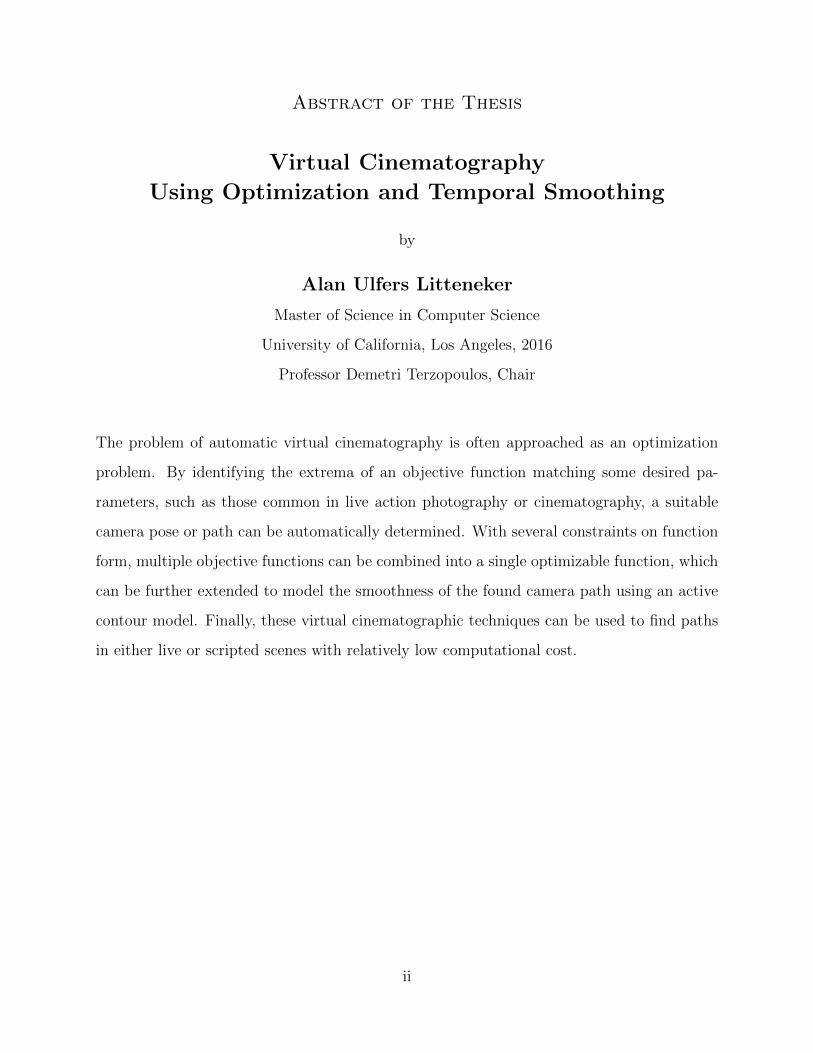
Abstract of the Thesis

Virtual Cinematography

Using Optimization and Temporal Smoothing

by

Alan Ulfers Litteneker

Master of Science in Computer Science

University of California, Los Angeles, 2016

Professor Demetri Terzopoulos, Chair

The problem of automatic virtual cinematography is often approached as an optimization

problem. By identifying the extrema of an objective function matching some desired pa-

rameters, such as those common in live action photography or cinematography, a suitable

camera pose or path can be automatically determined. With several constraints on function

form, multiple objective functions can be combined into a single optimizable function, which

can be further extended to model the smoothness of the found camera path using an active

contour model. Finally, these virtual cinematographic techniques can be used to find paths

in either live or scripted scenes with relatively low computational cost.

ii

The thesis of Alan Ulfers Litteneker is approved.

Song-Chun Zhu

Joseph M. Teran

Demetri Terzopoulos, Committee Chair

University of California, Los Angeles

2016

iii

Insert dedication here.

iv

Table of Contents

1 Introduction . . . . . . . . . . . . . . . . . . . . . . . . . . . . . . . . . . . . . . 1

1.1 Related Work . . . . . . . . . . . . . . . . . . . . . . . . . . . . . . . . . . . 3

1.2 Objective and Contributions . . . . . . . . . . . . . . . . . . . . . . . . . . . 3

1.3 Thesis Overview . . . . . . . . . . . . . . . . . . . . . . . . . . . . . . . . . . 4

2 Virtual Cinematography System . . . . . . . . . . . . . . . . . . . . . . . . . 5

2.1 Objective Functions . . . . . . . . . . . . . . . . . . . . . . . . . . . . . . . . 5

2.2 Predefined Shot Parameters . . . . . . . . . . . . . . . . . . . . . . . . . . . 6

2.2.1 Visibility . . . . . . . . . . . . . . . . . . . . . . . . . . . . . . . . . . 7

2.2.2 Shot Size . . . . . . . . . . . . . . . . . . . . . . . . . . . . . . . . . 10

2.2.3 Relative Angles . . . . . . . . . . . . . . . . . . . . . . . . . . . . . . 11

2.2.4 Rule of Thirds . . . . . . . . . . . . . . . . . . . . . . . . . . . . . . . 13

2.2.5 Look Space . . . . . . . . . . . . . . . . . . . . . . . . . . . . . . . . 14

2.3 Temporal Objective Functions . . . . . . . . . . . . . . . . . . . . . . . . . . 15

2.4 Optimization Techniques . . . . . . . . . . . . . . . . . . . . . . . . . . . . . 16

2.5 Parameter Satisfaction . . . . . . . . . . . . . . . . . . . . . . . . . . . . . . 18

3 Experiments and Results . . . . . . . . . . . . . . . . . . . . . . . . . . . . . . 20

3.1 Use Cases . . . . . . . . . . . . . . . . . . . . . . . . . . . . . . . . . . . . . 20

3.1.1 Scripted Scenarios . . . . . . . . . . . . . . . . . . . . . . . . . . . . 20

3.1.2 Live Scenarios . . . . . . . . . . . . . . . . . . . . . . . . . . . . . . . 21

3.2 Results . . . . . . . . . . . . . . . . . . . . . . . . . . . . . . . . . . . . . . . 23

3.2.1 Speed . . . . . . . . . . . . . . . . . . . . . . . . . . . . . . . . . . . 23

v

3.2.2 Camera Paths . . . . . . . . . . . . . . . . . . . . . . . . . . . . . . . 25

4 Conclusion . . . . . . . . . . . . . . . . . . . . . . . . . . . . . . . . . . . . . . . 27

4.1 Discussion and Future Work . . . . . . . . . . . . . . . . . . . . . . . . . . . 27

Bibliography . . . . . . . . . . . . . . . . . . . . . . . . . . . . . . . . . . . . . . . 29

vi

List of Figures

2.1 A frame with too much headroom, as chosen by our system. . . . . . . . . . 8

2.2 Example close-up and wide shots, chosen by our system . . . . . . . . . . . . 11

2.3 Example low height angle and profile angle shots chosen by our system . . . 12

2.4 Example frame with inadequate look space chosen by our system . . . . . . . 14

3.1 An overhead of a simple moving scene. . . . . . . . . . . . . . . . . . . . . . 24

3.2 An overhead of a far less simple scene. . . . . . . . . . . . . . . . . . . . . . 25

3.3 Overhead of the same scene with and without smoothing . . . . . . . . . . . 26

vii

Acknowledgments

Insert acknowledgements here.

viii

CHAPTER 1

Introduction

The problem of virtual cinematography is one of the oldest in 3D computer graphics. The

settings chosen for a virtual camera intrinsically affect both what objects are visible and how

the viewer perceives them.

In general, the goal of any declarative virtual cinematography system is to select camera

settings which match a set of parameters for the final rendered frame. If the desired param-

eters are merely descriptions of simple geometric relationships, this problem can be solved

by very fast established algorithms employing analytical mathematical functions (look at

matrices, arc balls, etc.).

However, the demands of real world applications are rarely so simple. Modeling even

the simplest of photographic and cinematographic techniques require much more complex

parameters, many of which are difficult to quantify at best (Datta and et al., 2006). Given

the incredible subjectivity of these art forms, users may frequently disagree both on how well

a frame matches a particular aesthetic, and on the relative importance of aesthetic properties

in a frame.

As such, virtual cinematography for scenes which are planned before delivery to the

viewer, such as with 3D animated films made popular by companies such as Pixar, is generally

solved manually by a human artist. However, when a scene is even partially unknown, such

as when playing a video game or viewing a procedurally generated real-time animation, some

sort of automatic virtual cinematography system must be used.

Several researchers have developed systems to this end (Christie and et al., 2005). All

attempt to identify a camera pose which matches a desired set of shot parameters; however,

1

they differ wildly in methodology. Some operate using purely algebraic solvers, others using

optimization techniques. Some rely on hard boolean constraints, others on continuous objec-

tive functions. Some attempt to identify the entirety of the satisfactory volume of solutions,

while others look for a single optimal solution.

Generally speaking, the differences in these systems tend to stem from the demands of the

intended application. Systems which do not rely on optimization techniques tend to be very

limited in their allowed expressiveness, but incur almost no computational cost. Systems

with boolean constraints can be very good at handling over-constrained parameter sets, but

tend to require computationally expensive stochastic solvers providing relatively inaccurate

solution approximations. Systems with continuous objective functions are generally faster

and more accurate, but require much more sensitive configuration and provide poor support

for over-constrained parameter sets.

As with many problems in computer science, this largely comes down to a question of

speed versus accuracy. Reducing the threshold for parameter satisfaction causes the volume

of satisfactory solutions to grow, and therefore allows a simpler algorithm to find a solution

faster. As this threshold is increased, or if the shot is over-constrained, the volume of

satisfactory solutions shrinks, requiring increasingly expensive computation to locate any

edge.

The type of system with which our research is concerned uses continuous objective func-

tions and optimization-based solvers. This was chosen so as to allow for high-quality solutions

for expressive parameters at a computational cost amenable to both real-time and planning

scenarios. We further introduce a set of shot parameters based on common cinematographic

aesthetic rules, a class of objective function that allows for a simple combination of parame-

ters as a weighted sum, and a method for modeling the temporal smoothness of the camera

path.

2

1.1 Related Work

As previously mentioned, there has been an incredibly diverse set of systems developed in

this field. The following are some of the projects most relevant to our work:

Beginning in the early 1970s, Blinn (1988) and others developed several mathematically

explicit models to support very fast algebraic solvers, principally used for the production

of “space movies.”1 However, these models were very limited in their expressiveness, each

designed for a very specific application and virtually unusable outside of it.

“Through-the-lens Camera Control” (Gleicher and Witkin, 1992) generalized several of

these more complex models into a unified optimization-based method that could solve for

a combination of soft constraints, such as having multiple points appear at specific screen

positions. However, as this too relied on analytical solvers, it too was incapable of handling

many types of constraints, including occlusions.

Several years later, systems such as CamDroid (Drucker and Zeltzer, 1995) were developed

that employed continuous optimization methods with complex state transitions, but were

nevertheless capable of running in real time. Issues such as the sensitive nature of the shot

weighting and difficulty with over-constraining led to the development of boolean constraint

systems such as ConstraintCam (Bares and et al., 2000), as well as stochastic optimization

techniques allowing interactive-time solutions that can be interpolated to approximate a

real-time solution (Burelli and et al, 2008; Abdullah and et al., 2011).

1.2 Objective and Contributions

The goal of this research is to develop a set of tools to find a temporally smooth camera

pose or path which satisfies a user specified set of shot parameters. In order to support as

expressive of shot parameters as possible, we introduce a standardized type of continuous

shot objective function which allows for a relatively simple combination of parameters. By

1As Blinn himself amusingly described it.

3

evaluating how well a particular pose or path matches the parameters as a scalar function

with certain constraints, this problem of camera control can be numerically solved using

relatively standard multivariate optimization techniques, such as simulated annealing and

gradient descent.

As the optimal camera path defined by these objective functions may not be temporally

smooth, active contour models are used to ensure a user specified amount of smoothness.

This research also introduces a set of predefined parameter types and corresponding

objective functions to allow the user to parameterize their desired shot in terms of common

live action cinematographic aesthetics, including shot size, relative angles, visibility, frame

bounds, occlusion, rule of thirds, and look space.

All of these techniques are implemented into a prototype system that is then evaluated

using both scripted and live scenarios among a number of different types of parameter sets.

1.3 Thesis Overview

The remainder of this thesis is organized as follows:

Chapter 2 presents the technical details of our virtual cinematography system. This

includes the objective functions, the predefined shot parameters, and the temporal objective

functions, optimization techniques employed to satisfy the parameters.

Chapter 3 reports on our experiments and results. We discuss several use cases and

document the performance of our system.

Chapter 4 concludes the thesis with a discussion of the efficacy and limitations of our

system and promising avenues for future work.

4

CHAPTER 2

Virtual Cinematography System

2.1 Objective Functions

In order to find a camera pose which matches the desired shot parameters, our system must

be able to evaluate how well a particular camera pose matches the given shot parameters.

This is done with an objective function f : RN 7→ R for each shot parameter. For notational

simplicity, these functions will be denoted as f(x) despite requiring different numbers and

types of parameters. Each function must meet the following criteria:

• Any optimal solution for shot i parameter must match argminx f(x).

• It must be that f(x) ≥ 0 and argminx f(x) = 0.

• Each rule should be as continuous as possible, such that limx→c f(x) = f(c) and

limx→cdf(x)dx

= df(c)dx

. As explored in Section 2.2, this is not always possible.

With an objective function matching these criteria, finding a camera pose that exactly

matches a given shot parameter is simply a matter of finding a minimum for f(x). As

minima cannot be identified analytically for many function types, our system attempts to

find approximate minima using numerical methods, as discussed in Section 2.4.

Furthermore, combining multiple shot parameters into a single objective function be-

comes a simple matter of computing the weighted sum of the their objective functions

f(x) =∑n

i=1 αifi(x), a strategy that critically allows for compromises between shot pa-

rameters for which the global minima do not precisely intersect. The influence of each

parameter can be tuned by adjusting the values of α.

5

All of the functions used are point based, meaning that all details of the scene are

collected in the form of observing the position, orientation, etc., of specific points connected

to objects of interest in the scene. This requires that complex elements in the scene be

represented by multiple points. This point-based model varies from the explicit geometric

models (Bares and et al., 2000; Jardillier and Langunou, 1998), where each camera pose is

evaluated based on observations of geometric primitives approximating complex objects, as

well as from rendering-based methods (Burelli and et al, 2008; Abdullah and et al., 2011),

where each camera pose is evaluated by analyzing a full rendering of the scene from that

pose.

2.2 Predefined Shot Parameters

While almost any valid objective function can be input by the user, our system provides

a set of predefined shot parameter types to support common cinematic and photographic

compositional aesthetics. These mimic the types of shot descriptions commonly used on

“shot lists” in the preproduction of a film by live-action directors and cinematographers.

While these parameters allow for many different shot descriptions, they are neither ex-

haustive nor are their common reasons for use without exception. Many additionally require

some form of contextually or behaviorally aware decision making before they will be valid.

For example, the relative angle constraints require as input a desired angle value, which our

current system is wholly incapable of automatically determining.

Although our current system does not provide functionality to automatically generate a

set of parameters for a given scene, the intention of this available parameter set is that a user

with a passing familiarity with the common types of shot descriptions used in cinematography

would be able to input a set of parameters that our system could use to automatically find

the desired camera pose.

Aside from a number of utility parameters (e.g., ensure the camera is not upside down),

our system currently only has automatic support for the parameters listed in this section, al-

6

though any additional objective function that matches the constraints outlined in Section 2.1

and operates on the variables of the rest of our system can be input as either a new function

or a combination of the existing functions.

While the components of our system integrated from the Unreal Engine rely on its partic-

ular coordinate system (left-handed, z-up, etc.), the functions listed here are written to be as

generic as possible. As several rules require the projection of a point on to the image plane,

the function Π(R3) → R2 is used to denote such a projection from world space to screen

space, where any point p that will appear in frame will have |v| ≤ 1,∀v ∈ Π(p). Note that

this projection function must have knowledge of the current camera position, orientation,

field of view, etc., which are not explicitly listed as parameters for many functions.

The following sections summarize the types of shot parameters used, briefly explain their

common artistic or contextual purpose, and provide the corresponding objective function:

2.2.1 Visibility

Bluntly put, objects the viewer should see must appear on screen. However, this apparently

simple behavior requires two different types of parameters, which are labeled here as frame

bounds and occlusion, both of which must be satisfied for an object to be visible.

2.2.1.1 Frame Bounds

The frame bounds rule is quite simply that any point that the user desires to be visible must

appear inside the bounds of the frame. In many circumstances, some points are commonly

required to be inset from the edge of the frame, a property commonly called headroom in

live action cinematography. For human subjects, too much room between the top of the

head and the edge of the frame causes the subject to appear small and insignificant, while

too little causes the subject to appear restricted and boxed in (Brown, 2013, p. 52).

Given world space point p and constants xlow < xhigh, where −xlow = xhigh = 1 ensures a

point is simply in frame and 0 < (|xlow|, xhigh) < 1 will produce headroom, the frame-bounds

7

Figure 2.1: A frame with too much headroom, as chosen by our system.

rule can be evaluated as follows:

f(p) =∑

x∈Π(p)

g(x), (2.1)

where

g(x) =

(x− xlow)2 x < xlow;

0 xlow ≤ x ≤ xhigh;

(x− xhigh)2 x > xhigh.

(2.2)

2.2.1.2 Occlusion

The occlusion rule is quite simply that there must be an unoccluded line of sight from the

camera to an object that the user desires to be visible. A common distinction is made

between clean shots where all of an object is unoccluded and dirty shots where only part of

object is unoccluded.

8

Unfortunately, building a suitable objective function for occlusion is much more compli-

cated. Unlike the all the other rules, evaluating whether a point is occluded is an observation

about the geometry of the scene as a whole and, as such, it cannot be defined in the same

concise analytic style as the rest of the functions. Furthermore, there will be a discontinuity

in any direct function at the boundary of occlusion, which does not meet the smoothness

requirements outlined in Section 2.1.

To address these issues, our system provides an n-dimensional linear interpolator that,

given camera position c and point position p, can be expressed mathematically as follows:

f(c) = f3(c), (2.3)

where

fi(c) =cai − ci

cbi − ca

i

fi−1(cb) +1− ca

i + ci

cbi − ca

i

fi−1(ca). (2.4)

Here, ca and cb are the closest sample locations on axis i such that cai ≤ ci, cb

i ≥ ci, and

caj = cb

j = cj,∀j 6= i, and

f0(c) = B(c,p), (2.5)

where

B(c,p) =

1 if the line segment from c to p is occluded;

0 if the line segment from c to p is not occluded.

(2.6)

As this function is not analytically differentiable, differentiation is computed numerically as

df(x)dx≈ f(x+∆x)−f(x)

∆xusing a small ∆x of about 1 cm virtual scale.

In an attempt to improve smoothness, our system supports convolution by a Gaussian

kernel to the samples of the interpolator, which can be expressed mathematically as changing

f0(c) to

f0(c) =1√

2πσ2h3(c). (2.7)

9

Here,

hi(c) =

K/2∑j=−K/2

e−(j∆i)

2

2σ2 hi−1(c+j∆iUi), (2.8)

where ∆ is the set of convolution step sizes, U is the set of bases for c, and h0(c) = B(c,p).

Of course, this blurring comes at a cost. Firstly, it requires many more ray casts than its

unblurred counterpart, decreasing overall efficiency. Secondly, this blurring can cause smaller

occluding elements to be ignored, a problem which partially comes down to the choice of

constants σ, ∆, and K. Increasing the size of the kernel K and decreasing the values of ∆ will

create a smoother, more continuous approximation, but will require more computation time.

Therefore, selecting suitable values for these functions is a difficult and critical problem; we

are not currently aware of a solution better than trial and error.

To ensure that multiple points S = {p1, . . . ,pn} are unoccluded, we further modify

h0(c) to h0(c) =∑n

j=1 wjB(c,pj). By varying the relative weights wi, the likelihood of more

important points (e.g., the eyes of a character versus their necktie) becoming occluded in the

frame can be drastically reduced. Furthermore, a dirty shot can be modeled by borrowing

g(x) from the frame bounds rule, and modifying h0(c) to h0(c) = g(∑n

j=1wiB(c,pi))

,

where xlow and xhigh are chosen to correspond to the desired amount of occlusion.

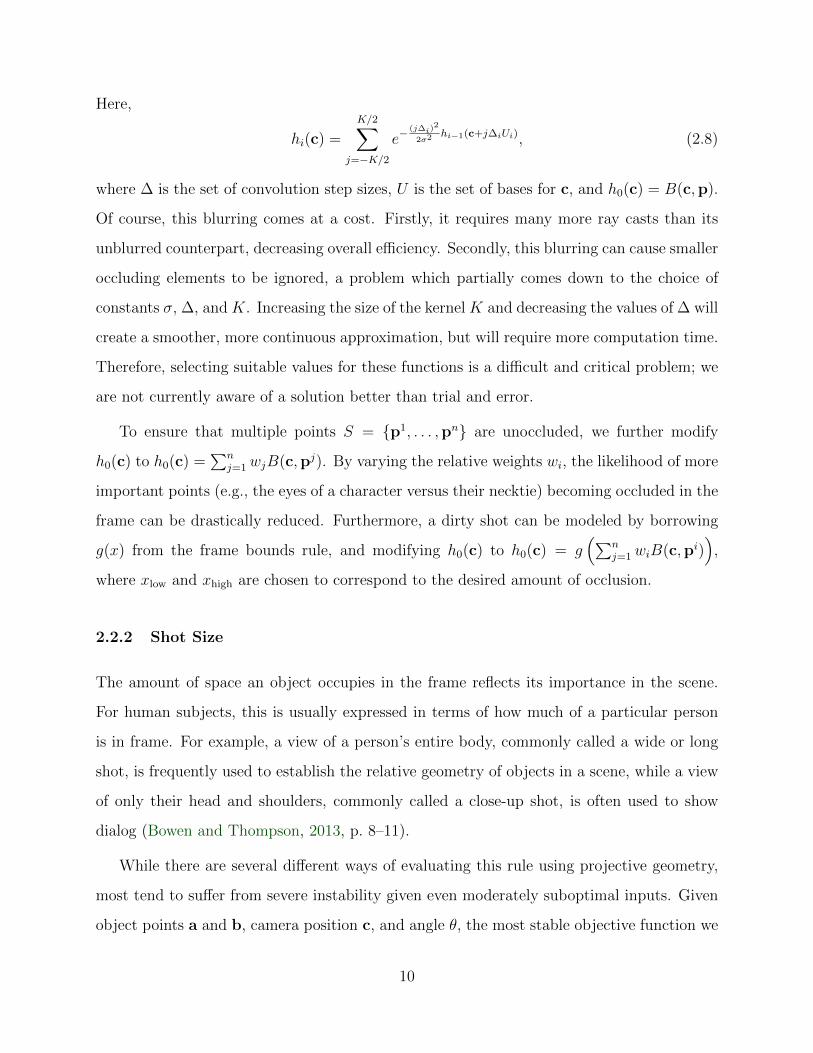
2.2.2 Shot Size

The amount of space an object occupies in the frame reflects its importance in the scene.

For human subjects, this is usually expressed in terms of how much of a particular person

is in frame. For example, a view of a person’s entire body, commonly called a wide or long

shot, is frequently used to establish the relative geometry of objects in a scene, while a view

of only their head and shoulders, commonly called a close-up shot, is often used to show

dialog (Bowen and Thompson, 2013, p. 8–11).

While there are several different ways of evaluating this rule using projective geometry,

most tend to suffer from severe instability given even moderately suboptimal inputs. Given

object points a and b, camera position c, and angle θ, the most stable objective function we

10

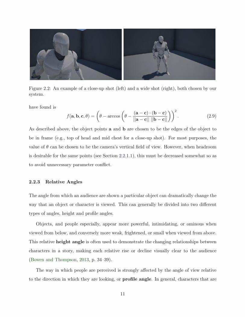
Figure 2.2: An example of a close-up shot (left) and a wide shot (right), both chosen by oursystem.

have found is

f(a,b, c, θ) =

(θ − arccos

(θ − (a− c) · (b− c)

||a− c|| ||b− c||

))2

. (2.9)

As described above, the object points a and b are chosen to be the edges of the object to

be in frame (e.g., top of head and mid chest for a close-up shot). For most purposes, the

value of θ can be chosen to be the camera’s vertical field of view. However, when headroom

is desirable for the same points (see Section 2.2.1.1), this must be decreased somewhat so as

to avoid unnecessary parameter conflict.

2.2.3 Relative Angles

The angle from which an audience are shown a particular object can dramatically change the

way that an object or character is viewed. This can generally be divided into two different

types of angles, height and profile angles.

Objects, and people especially, appear more powerful, intimidating, or ominous when

viewed from below, and conversely more weak, frightened, or small when viewed from above.

This relative height angle is often used to demonstrate the changing relationships between

characters in a story, making each relative rise or decline visually clear to the audience

(Bowen and Thompson, 2013, p. 34–39).

The way in which people are perceived is strongly affected by the angle of view relative

to the direction in which they are looking, or profile angle. In general, characters that are

11

Figure 2.3: An example of a shot from a low height angle (left) and a profile angle (right)chosen by our system.

viewed directly from the front are felt to be more connected to the viewer than characters

viewed in profile, mimicking the way humans tend to face directly towards things they are

focused on (Bowen and Thompson, 2013, p. 40–43).

Given object point p, camera position c, unit object up direction u, and desired angle θ

relative to unit object look direction d, the objective function for height angle (2.10) is

f(p, c,u, θ) =

(θ − arccos

(p− c

||p− c||· u))2

, (2.10)

while for profile angle (2.11) it is

f(p, c,u,d, θ) =

(θ − arccos

(p− u((p− c) · u)− c

||p− u((p− c) · u)− c||· d))2

. (2.11)

These two functions are very similar, but differ in the shape of the optimal solutions. Ef-

fectively, the set of optimal inputs for the height angle (2.10) function form a cone whose

apex is the object point and whose axis is the up direction. Meanwhile, the set of optimal

inputs for the profile angle function (2.11) form a pair of planes that intersect at the object

point, have a line of intersection which is the object up direction, and are symmetric across

the object look direction.

12

2.2.4 Rule of Thirds

A standard (and very old) rule of thumb in photographic composition is to place important

objects near the third lines, both vertical and horizontal, in the frame. The most important

objects in the scene are frequently placed nearest to the four intersections of these lines in

the camera frame (Brown, 2013, p. 51).

All of the example frames shown in this section conform to this parameter. Given a point

in world space p as well as constants 0 ≤ x0 ≤ 1 and 0 < a ≤ 1, one formulation can be

formed as follows:

f(p) =∑

x∈Π(p)

g(x) (2.12)

where

g(x) = h(x)− h(x0). (2.13)

Here

h(x) =(x+ b)2

(x+ b)2 + a+

(x− b)2

(x− b)2 + a(2.14)

and

b =

√√√√2 (x20 − a) +

√4 (x2

0 − a)2

+ 12 (x20 + a)

2

6. (2.15)

To use the standard third lines, x0 should be set to 13. Selecting a value for a is a bit trickier,

as too high a setting causes the function only to affect points in the immediate vicinity

on-screen while too low a setting can cause the penalty for |x| < x0 to decrease significantly.

This formulation has an issue in that it penalizes points far from x0 equally as limx→±∞ g(x) =

2. In some applications this “flatness” is desirable; for example, if there is an object that is

not required in a shot but that should be placed on the third lines when it is in frame.

A “non-flat” function can be formulated much more simply as g(x) = x4

x40− 2x2

x20

+ 1. This

has the same double minimum shape as before, but penalizes inputs for which |x| ≤ x0

much more lightly than those for which |x| > x0. Because of the exponential nature of this

asymmetric penalization, this formulation tends to be trickier to balance in a full parameter

13

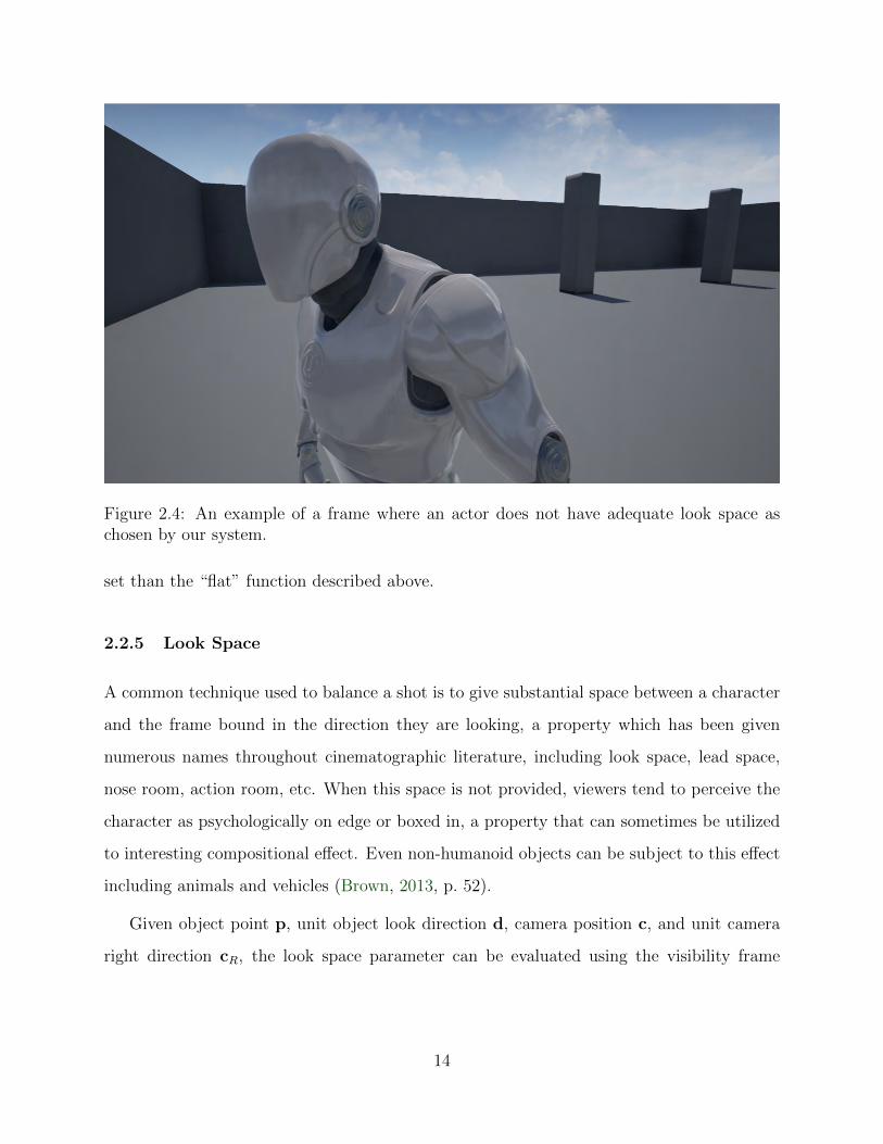
Figure 2.4: An example of a frame where an actor does not have adequate look space aschosen by our system.

set than the “flat” function described above.

2.2.5 Look Space

A common technique used to balance a shot is to give substantial space between a character

and the frame bound in the direction they are looking, a property which has been given

numerous names throughout cinematographic literature, including look space, lead space,

nose room, action room, etc. When this space is not provided, viewers tend to perceive the

character as psychologically on edge or boxed in, a property that can sometimes be utilized

to interesting compositional effect. Even non-humanoid objects can be subject to this effect

including animals and vehicles (Brown, 2013, p. 52).

Given object point p, unit object look direction d, camera position c, and unit camera

right direction cR, the look space parameter can be evaluated using the visibility frame

14

bounds objective function fvis(p), as follows:

f(p) = fvis

(Π(p) +

Π(p + d)− Π(p)

||Π(p + cR)− Π(p)||

), (2.16)

where, again, Π indicates the projection from world space to screen space.

2.3 Temporal Objective Functions

While the objective functions as already defined are capable of determining how well a

camera pose matches a set of shot parameters for a particular moment of time, evaluating

the same functions over an entire camera path requires the parameterization of x over time

to x(t), which can be evaluated as∫f(x(t))dt, which in turn must be approximated using

keyframes as∑f(x(t)) as our system operates in discrete time.

However, this simple temporal objective function completely fails to model the inertia and

momentum viewers expect from real world cameras. Generally speaking, any camera path

that is not smooth tends to be perceived as unnervingly artificial and mechanical. This issue

can be addressed by extending our given model with an active contour model (Kass et al.,

1988). In this augmented model, our system attempts to minimize the energy functional

E(x(t)) = Eint(x(t)) + Eext(x(t)) (2.17)

comprising an internal energy

Eint(x(t)) =1

2

(α|x(t)|2 + β|x(t)|2

), (2.18)

where α and β are given constants and the overstruck dots denote differentiation with respect

to t, and an external energy

Eext(x(t)) = c(t)f(x(t)), (2.19)

where c(t) is the certainty in the data.

15

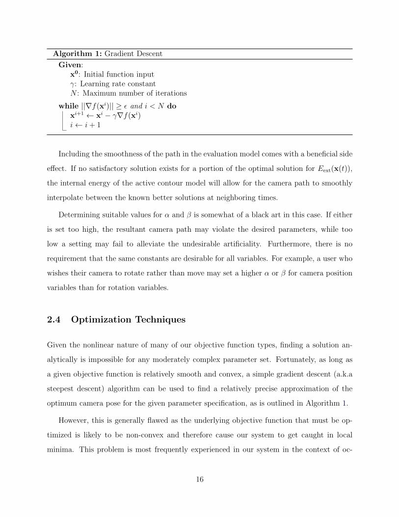
Algorithm 1: Gradient Descent

Given:x0: Initial function inputγ: Learning rate constantN : Maximum number of iterations

while ||∇f(xi)|| ≥ ε and i < N doxi+1 ← xi − γ∇f(xi)i← i+ 1

Including the smoothness of the path in the evaluation model comes with a beneficial side

effect. If no satisfactory solution exists for a portion of the optimal solution for Eext(x(t)),

the internal energy of the active contour model will allow for the camera path to smoothly

interpolate between the known better solutions at neighboring times.

Determining suitable values for α and β is somewhat of a black art in this case. If either

is set too high, the resultant camera path may violate the desired parameters, while too

low a setting may fail to alleviate the undesirable artificiality. Furthermore, there is no

requirement that the same constants are desirable for all variables. For example, a user who

wishes their camera to rotate rather than move may set a higher α or β for camera position

variables than for rotation variables.

2.4 Optimization Techniques

Given the nonlinear nature of many of our objective function types, finding a solution an-

alytically is impossible for any moderately complex parameter set. Fortunately, as long as

a given objective function is relatively smooth and convex, a simple gradient descent (a.k.a

steepest descent) algorithm can be used to find a relatively precise approximation of the

optimum camera pose for the given parameter specification, as is outlined in Algorithm 1.

However, this is generally flawed as the underlying objective function that must be op-

timized is likely to be non-convex and therefore cause our system to get caught in local

minima. This problem is most frequently experienced in our system in the context of oc-

16

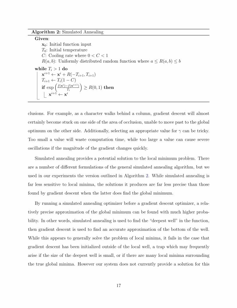
Algorithm 2: Simulated Annealing

Given:x0: Initial function inputT0: Initial temperatureC: Cooling rate where 0 < C < 1R(a, b): Uniformly distributed random function where a ≤ R(a, b) ≤ b

while Ti > 1 doxi+1 ← xi +R(−Ti+1, Ti+1)Ti+1 ← Ti(1− C)

if exp(

f(xi)−f(xi+1)Ti

)≥ R(0, 1) then

xi+1 ← xi

clusions. For example, as a character walks behind a column, gradient descent will almost

certainly become stuck on one side of the area of occlusion, unable to move past to the global

optimum on the other side. Additionally, selecting an appropriate value for γ can be tricky.

Too small a value will waste computation time, while too large a value can cause severe

oscillations if the magnitude of the gradient changes quickly.

Simulated annealing provides a potential solution to the local minimum problem. There

are a number of different formulations of the general simulated annealing algorithm, but we

used in our experiments the version outlined in Algorithm 2. While simulated annealing is

far less sensitive to local minima, the solutions it produces are far less precise than those

found by gradient descent when the latter does find the global minimum.

By running a simulated annealing optimizer before a gradient descent optimizer, a rela-

tively precise approximation of the global minimum can be found with much higher proba-

bility. In other words, simulated annealing is used to find the “deepest well” in the function,

then gradient descent is used to find an accurate approximation of the bottom of the well.

While this appears to generally solve the problem of local minima, it fails in the case that

gradient descent has been initialized outside of the local well, a trap which may frequently

arise if the size of the deepest well is small, or if there are many local minima surrounding

the true global minima. However our system does not currently provide a solution for this

17

problem.

Optimizing for camera paths using these algorithms is a straightforward extension of

optimizing for static poses. Without the smoothing from an active contour model, optimizing

on a temporal objective function is a simple matter of running the optimization algorithms

locally on each frame. Optimizing with smoothing is somewhat more involved. Each time

interval must first be initialized with a locally computed rough optimum that ignores the

smoothing, then gradient descent can be used such that every component of E(x(t)) is

computed for every time step t before any new values can be set.

2.5 Parameter Satisfaction

Thus far all of the techniques discussed have operated entirely continuously, and provide little

insight into whether the solution discovered actually satisfies the provided shot parameters.

For example, it is difficult to tell whether an evaluation score of 1.0 is close enough to the

theoretical minimum of 0.0 that the user would describe the resultant frame as matching

their desired parameters. Consider the following hypothetical scenarios:

A user inputs an objective function which specifies that the camera be in front of two

different actors standing side-by-side, but if they face in opposite directions no adequate

solution may be possible. Depending on the exact parameter set, the continuous optimizers

described above will likely find a solution that is directly between the actors with neither in

frame, which is clearly not a viable solution. Alternatively, it may find a solution that views

both actors from the side, which may also be unsatisfactory.

A user of our system specifies that it should interpolate between two different parameter

sets; for example, panning from one actor to another. If the two parameter specifications

are even moderately dissimilar, one or both is very likely to be unsatisfied at every instant

of the shot. However, unlike the previous example, the solution found by the continuous

optimizers may be acceptable to the user.

A user specifies that the camera should follow an actor from the side as he walks past

18

a column, causing part of the optimal camera path to likely have an occluded view of the

actor depending on smoothing factors. Whether this period of occlusion will be acceptable

to the user is a question of contextual information that our current system lacks.

In general, one appealing conceptual solution would be to provide an automatic boolean

test to answer this question. A simple way to run such a test is to select a canonical boundary

state for each parameter, and simply compare the value of the parameter’s function at that

boundary state; formally, ∀fi(x) ∃bi s.t. fi(x) ≤ fi(bi) only when the parameter is satisfied.

By taking the logical conjunction of multiple tests, a boolean test for all parameters can be

formed.

For parameters like visibility, this boundary state is simply that points are in frame and

unoccluded for a given camera pose. However, determining a reasonable boundary state for

parameter types like relative angles and the rule of thirds is far less straightforward. As

such, our system does not currently attempt to provide automatic boundary specification,

instead simply allowing users to specify boundary states. This allows for simple warnings to

the user when the automatically found camera pose or path fails their tests.

19

CHAPTER 3

Experiments and Results

In this chapter, we first consider the various use cases supported by our virtual cinematog-

raphy system and then present our results.

3.1 Use Cases

While there are many different ways of utilizing the cinematographic tools outlined here, our

system supports two primary categories of use cases, which are labeled as scripted and live

scenarios.

3.1.1 Scripted Scenarios

In a scripted scenario, our system attempts to find a satisfactory camera path for a pre-

planned scene before any part of it is to be displayed to the viewer. As this is an offline

operation, our system can take as much time as is necessary to find a satisfactory solution.

Furthermore, complete knowledge of all past, current, and future states of the scene are

available at every instant of time. This is analogous to the planning and shooting of a live

action scripted film, or to 3D animation of the sort made popular by companies such as

Pixar.

Scripted scenarios are handled quite simply by the tools already outlined. For every

frame in a scene with a user input parameter set, our system employs the given optimization

techniques until all parameters are satisfied or a maximum search time is reached. Without

smoothing, our system locally optimizes every frame in two stages, where a brief phase of

20

simulated annealing attempts to find the neighborhood of the global optimum, followed by a

phase of fine tuning by gradient descent. With smoothing, the same two stage optimization

is run to initialize the camera at every frame, followed by the active contour model gradient

descent as outlined at the end of Section 2.3.

3.1.2 Live Scenarios

In a live scenario, the goal of our system is to find a camera pose for the current instant of

time given complete knowledge of the past and current states of the scene, but without any

direct knowledge of the future. Furthermore, this is an operation online with the playback

of the scene, and therefore our system must be able to find a satisfactory solution at a time

amenable to the viewer’s desired frame rate. This is analogous to the shooting of unscripted

live action documentary or news material, or to video game camera control.

Without smoothing by an active contour model, this is a relatively simple operation. The

first frame camera pose is set either by the user or via a stochastic search method such as

simulated annealing, then gradient descent is run every frame starting from the values of the

previous frame. This has the advantage of being a very fast method for producing optima

of decent quality and a reasonably smooth overall camera path, as the smoothness of the

underlying objective function would suggest.

However, there are two significant problems. The first is that the camera can easily

become stuck at local minima, most commonly at the boundary of an area of occlusion.

As already mentioned, this is a common pitfall of gradient descent, which can be partially

addressed by including a simulated annealing optimization phase to each frame at the cost of

a reduced frame rate. The second problem is that this approach tends to chase the nearest

optimum at every frame, rather than accurately locate it, even if the tracked actors are

moving along straight lines. Nevertheless, this approach is appropriate for many simple

scenes.

Live scenarios with smoothing are significantly trickier as, in order for the active contour

21

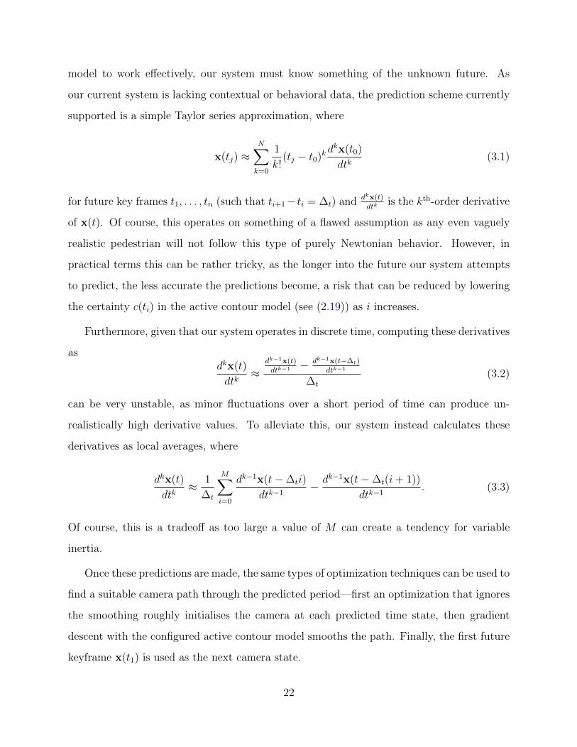
model to work effectively, our system must know something of the unknown future. As

our current system is lacking contextual or behavioral data, the prediction scheme currently

supported is a simple Taylor series approximation, where

x(tj) ≈N∑k=0

1

k!(tj − t0)k

dkx(t0)

dtk(3.1)

for future key frames t1, . . . , tn (such that ti+1− ti = ∆t) and dkx(t)dtk

is the kth-order derivative

of x(t). Of course, this operates on something of a flawed assumption as any even vaguely

realistic pedestrian will not follow this type of purely Newtonian behavior. However, in

practical terms this can be rather tricky, as the longer into the future our system attempts

to predict, the less accurate the predictions become, a risk that can be reduced by lowering

the certainty c(ti) in the active contour model (see (2.19)) as i increases.

Furthermore, given that our system operates in discrete time, computing these derivatives

asdkx(t)

dtk≈

dk−1x(t)dtk−1 − dk−1x(t−∆t)

dtk−1

∆t

(3.2)

can be very unstable, as minor fluctuations over a short period of time can produce un-

realistically high derivative values. To alleviate this, our system instead calculates these

derivatives as local averages, where

dkx(t)

dtk≈ 1

∆t

M∑i=0

dk−1x(t−∆ti)

dtk−1− dk−1x(t−∆t(i+ 1))

dtk−1. (3.3)

Of course, this is a tradeoff as too large a value of M can create a tendency for variable

inertia.

Once these predictions are made, the same types of optimization techniques can be used to

find a suitable camera path through the predicted period—first an optimization that ignores

the smoothing roughly initialises the camera at each predicted time state, then gradient

descent with the configured active contour model smooths the path. Finally, the first future

keyframe x(t1) is used as the next camera state.

22

3.2 Results

All of these tools and techniques were implemented in a single-threaded prototype camera

control system which was integrated with Unreal Engine 4.9, running online with the en-

gine’s standard game thread. Several different experimental scenes were then tested for both

scripted and live scenarios on a desktop machine with a 3.07 GHz quad-core processor and

an Nvidia GTX 980 graphics card.

For most experiments, each camera pose required that our system optimize over 5

variables—position in R3, yaw, and pitch. This required that each shot had a static user

specified field of view and aspect ratio. In principle, our system is capable of optimizing over

both static variables as well as camera roll, but changing these parameters mid-shot is less

common in standard cinematography.

3.2.1 Speed

Measuring the speed of our system for scripted scenarios is tricky as it entirely depends on

the tightness of the satisfaction boundaries. It should be noted that, for all scenes tested, a

keyframe rate of 40 per second was subjectively found to produce a decently smooth camera

path, and could keep up with the speed of motion reasonably well. For most of the scenes

tested, a satisfactory unsmoothed camera path could be found using approximately 200 iter-

ations of simulated annealing, followed by approximately 200 iterations of gradient descent,

taking about 1.15 seconds per frame. With smoothing, the same two-phase optimization can

be used to roughly locally optimize using about 50-75% of the iterations required without

smoothing, followed by 400-600 iterations of gradient descent with the active contour model

at a total cost of about 1.75 seconds per frame. Of course, the threshold for parameter sat-

isfaction is highly subjective, so another user on an identical machine may experience very

different performance.

The speed of live scenarios is easier to quantify. Again, there is a tradeoff between

processor time and solution quality, so a user willing to endure a lower frame rate can set a

23

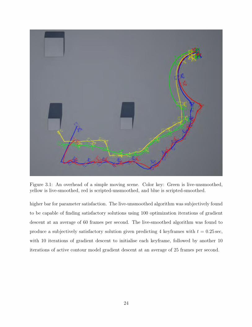
Figure 3.1: An overhead of a simple moving scene. Color key: Green is live-unsmoothed,yellow is live-smoothed, red is scripted-unsmoothed, and blue is scripted-smoothed.

higher bar for parameter satisfaction. The live-unsmoothed algorithm was subjectively found

to be capable of finding satisfactory solutions using 100 optimization iterations of gradient

descent at an average of 60 frames per second. The live-smoothed algorithm was found to

produce a subjectively satisfactory solution given predicting 4 keyframes with t = 0.25 sec,

with 10 iterations of gradient descent to initialise each keyframe, followed by another 10

iterations of active contour model gradient descent at an average of 25 frames per second.

24

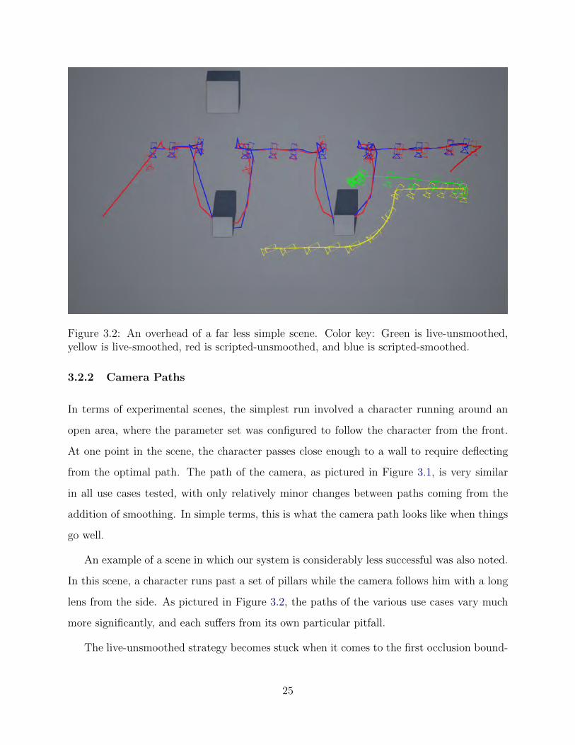
Figure 3.2: An overhead of a far less simple scene. Color key: Green is live-unsmoothed,yellow is live-smoothed, red is scripted-unsmoothed, and blue is scripted-smoothed.

3.2.2 Camera Paths

In terms of experimental scenes, the simplest run involved a character running around an

open area, where the parameter set was configured to follow the character from the front.

At one point in the scene, the character passes close enough to a wall to require deflecting

from the optimal path. The path of the camera, as pictured in Figure 3.1, is very similar

in all use cases tested, with only relatively minor changes between paths coming from the

addition of smoothing. In simple terms, this is what the camera path looks like when things

go well.

An example of a scene in which our system is considerably less successful was also noted.

In this scene, a character runs past a set of pillars while the camera follows him with a long

lens from the side. As pictured in Figure 3.2, the paths of the various use cases vary much

more significantly, and each suffers from its own particular pitfall.

The live-unsmoothed strategy becomes stuck when it comes to the first occlusion bound-

25

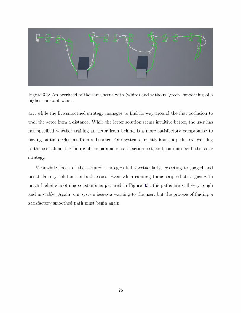
Figure 3.3: An overhead of the same scene with (white) and without (green) smoothing of ahigher constant value.

ary, while the live-smoothed strategy manages to find its way around the first occlusion to

trail the actor from a distance. While the latter solution seems intuitive better, the user has

not specified whether trailing an actor from behind is a more satisfactory compromise to

having partial occlusions from a distance. Our system currently issues a plain-text warning

to the user about the failure of the parameter satisfaction test, and continues with the same

strategy.

Meanwhile, both of the scripted strategies fail spectacularly, resorting to jagged and

unsatisfactory solutions in both cases. Even when running these scripted strategies with

much higher smoothing constants as pictured in Figure 3.3, the paths are still very rough

and unstable. Again, our system issues a warning to the user, but the process of finding a

satisfactory smoothed path must begin again.

26

CHAPTER 4

Conclusion

The research reported in this thesis has introduced several novel techniques for automatic

virtual cinematography. These include smooth objective functions which allow for the simple

combination of parameters by weighted summation as well as active contour models to model

camera path smoothness. These techniques have been implemented for, and tested in, both

live and scripted scenes, and were found to be capable of finding solutions in either real or

interactive time, depending on the specific strategy used. While these techniques have many

drawbacks and potential points of failure, their potential capabilities given further research

and development are considerable.

4.1 Discussion and Future Work

While there has been some anecdotal feedback from users of the current prototype, we

have not attempted to run a proper user study examining whether the rules and algorithms

devised here are satisfactory for the rigors of professional use. There are many common cine-

matographic rules that were not explored, including frame balance, leading lines, separation,

depth of field, and many more. Finding suitable objective functions for these rules would

make our system more expressive, but only if users are familiar with and want to use these

rules.

Additionally, the optimization techniques used here are almost certainly not optimal in

efficiency or efficacy. Some kind of continuation method with a stochastic gradient descent

would almost certainly be much more robust to local minima, and considerably faster. Ad-

27

ditionally, the proposal of Bares and et al. (2000) of developing a hybrid of continuous and

boolean constraints for efficient solvers may yield another significant advance.

There are also several unexplored questions stemming from the construction of the objec-

tive function itself. Is it possible to form a shot parameter specification for a planned scene

given contextual data? Alternatively, is it possible to automatically form an aesthetically

appealing shot specification in an unplanned scene using only behavioral context? Further-

more, can this constraint specification skill be acquired with machine learning? When no

satisfactory solution is found, is it possible to automatically find a better compromise by

modifying the parameters or weights, or by automatically adjusting actor blocking?

Furthermore, the ability to automatically adjust the blocking of actors may prompt a sig-

nificantly different approach towards optimization. In real world cinematography, the actors

are frequently blocked based on the physical constraints of the camera and environment in

conjunction with the content of the scene, a process that no existing system has attempted

to employ. Furthermore, while some virtual cinematography systems are aware of frame

properties such as brightness and contrast, to our knowledge no system has also attempted

to control the lighting of the scene so as to improve the aesthetic quality of the frame.

28

Bibliography

Abdullah, R. and et al. (2011). Advanced composition in virtual camera control. In Smart

Graphics. Springer, Berlin. 3, 6

Bares, W. and et al. (2000). Virtual 3D camera composition from frame constraints. In

Proc. 8th ACM International Conference on Multimedia. 3, 6, 28

Blinn, J. (1988). Where am I? What am I looking at? IEEE Computer Graphics and

Applications, 8(4):76–81. 3

Bowen, C. J. and Thompson, R. (2013). Grammar of the Shot. Taylor & Francis. 10, 11, 12

Brown, B. (2013). Cinematography: Theory and Practice: Image Making for Cinematograp-

ers and Directors. Taylor & Francis. 7, 13, 14

Burelli, P. and et al (2008). Virtual camera composition with particle swarm optimization.

In Smart Graphics. Springer, Berlin. 3, 6

Christie, M. and et al. (2005). Virtual camera planning: A survey. In Smart Graphics.

Springer, Berlin. 1

Datta, R. and et al. (2006). Studying aesthetics in photographic images using a compu-

tational approach. In Computer Vision – ECCV 2006, pages 288–301. Springer, Berlin.

1

Drucker, S. M. and Zeltzer, D. (1995). Camdroid: A system for implementing intelligent

camera control. In Proc. 1995 ACM Symposium on Interactive 3D Graphics. 3

Gleicher, M. and Witkin, A. (1992). Through-the-lens camera control. Computer Graphics,

26(2). (Proc. ACM SIGGRAPH ’92). 3

Jardillier, F. and Langunou, E. (1998). Screenspace constraints for camera movements: The

virtual cameraman. Computer Graphics Forum, 17(3). 6

29

Kass, M., Witkin, A., and Terzopoulos, D. (1988). Snakes: Active contour models. Interna-

tional Journal of Computer Vision, 1(4):321–331. 15

30