Image Reconstruction Using Bispectrum Speckle ... · Roberto Maria Caloi [email protected] Abstract: Vol. 14 No. 4 October 1, 2018 Journal of Double Star Observations Page 751 ... By

Vol. 14 No. 4 October 1, 2018 Page 750 Journal of Double Star Observations

1. Introduction

For rapid prototyping and deployment of all re-

quired calculations, I have used Matlab, which has pro-vided me a very good compromise between perfor-mance and ease of development.

2. Image Formation The image reconstruction process is essentially an

inverse problem, since the main task is to recover the

Image Reconstruction Using Bispectrum Speckle Interferometry: Application and First Results

Roberto Maria Caloi

[email protected]

Abstract:



original image based on the result of observations. Sev-eral noise sources make the recovering process subject to uncertainties and biases. In order to appreciate all the data and assumptions necessary to deal with these as-pects, it helps to review the main physical processes in-volved in the image formation on the detector that are later considered to recover the original image. Other re-finements could be evaluated, in particular on how to model the actual functioning of a real detector, but they are not considered here.

,

Given the incoming intensity distribution itλ(x, y),

the actual number of photons detected per pixel will depend also on the quantum nature of light and on the actual detector used, whose main characteristics are the following: level of dark current generation, quantum ef-ficiency, electronic read-out noise, electronic biases, presence of defects and hot pixels. These effects are par-ticularly important when the average total number of detected photons per speckle Nph is low, some hundreds or thousands to give an order of magnitude, and must be dealt with in order to avoid estimation biases (which do not disappear by simply increasing the number of record-ed images used in the data reduction process).

If itλ(x, y) is normalized so that its total value over

the image plane is one, the expected number of photoe-lectrons it

phe(x,y) is then given by

summing all three previous components and dividing by the detector gain G,

2 2

0

' '

'

x y

R

+

( ) ( ) ( ), , ,i x y o x y PSF x y = [1]

( )( )( ) ( ) ( )

( )

2, , 0, 1,

,

phet eADU

t

DC

P i x y l x y Ni x y

Gb x y

+ + =

[4]

[2] ( , ) ( , ) ( , )t ti x y o x y PSF x y =

[3] ( , ) ( , ) ( , )phe ph

t t thi x y N o x y PSF x y n = +



3. Power Spectrum Estimation A data cube {it

ADU(x)}Mt=1 of M short exposure

frames

{dtADU(x)}L

t=1 obtained with the telescope aperture cov-ered is needed. The first step in the image reconstruc-tion process requires the computation of the power spectrum, both its average and variance. Each frame it

ADU(x) is first corrected for the gain, G, the bias bDC(x) and the flat field l(x), to yield the actual photo-electrons plus read-out noise per pixel

It is subsequently cropped within a square

Nt

Here we assume that Ntth and Nt

dth have the same ex-pected values.

The discrete Fourier transform It(u) = DFT(it(x)) where u indicates the bi-

inherent in the de-tection process. Gordon and Buscher (2012) derived a formula for a bias-free power spectrum estimator St(u), when photon noise, thermal noise (dark current), and read-out noise are all taken into account. The main stated assumption in their study is that the various noise sources considered are independent and additive. Moreover the overall noise on different pixel positions

is assumed to be statistically independent. Under discrete Fourier transform conditions, which

hold in our case, their proposed estimator becomes

where x indicates the pixel position, it(x) the recorded intensity, and σe

2(x) is the read-out noise variance. Un-der the additional assumption that the read-out noise does not depend on the detector position, i.e. σe(x) = σe, equation 5 becomes

where Nt = Ntph + Nt

th is the total number of photo-electrons and thermal electrons per frame and Npix is the total number of pixels. By averaging St(u) we obtain an unbiased estimate of the power spectrum

where the operator ‹› represents averaging over the en-tire sequence of specklegrams. The sample variance of such estimate var(S) is then used to calculate the fre-quency dependent power spectrum standard deviation σS(u),

where M is the number of frames. The resulting power spectra has a central peak which is given by (Ñph

+ Ñth

)2

where Ñph is the average number of photo-electrons

per frame and Ñth = Ñdth is the average number of elec-trons generated by the thermal noise. By correcting the central peak component for the thermal noise, the final estimate of the power spectrum S(u) is obtained. No further correction is necessary outside the central peak if the thermal noise is spatially uncorrelated, so that its power spectrum is negligible for spatial frequencies different from zero.

The same analysis just described is repeated for a nearby reference star, which must be observed with similar seeing conditions as the object under study. Once we have estimated the object power spectrum Sobj(u) and its variance σ2

Sobj(u) as well as the refer-ence star’s power spectrum Sref(u) and its variance σ2

Sref(u), we can apply the standard procedure of speck-le interferometry (Labeyrie, 1970) which yields an esti-mate of the true object power spectrum |O(u)|2 = Sobj(u)/Sref(u) up to the telescope cut-off frequency, and its var-iance σ2

|O(u)|2

( )( ) ( )

( )

ADUt DC

t

Gi x b xi x

l x

−=

( )2 2( ) ( ) ( ) ( )t t t e

x

S u I u i x x= − + [5]

2 2( ) ( )t t t pix eS u I u N N = − − [6]

2 2( ) pix eS I u N N = − − [7]

( )( ) var ( ) /S u S u M = [8]



from which the image could be reconstructed by applying the inverse Fourier transform.

4. Bispectrum Estimation Let us first recall its definition. Given an intensity

distribution i(x) and its Fourier transform I(u), the bispectrum is defined as I(3)(u,v) =

complex conjugate of I(u). Similarly, for the true object intensity distribution o(x) we have O(3)(u, v) = O(u)O(v)O*(u + v) = |O(3)(u,v)| exp[βO(3)(u,v)]. It has been shown by Lohmann et al. (1983) that the phase of the time-averaged bispectrum of the atmospheric transfer function is close to zero while its modulus is not and, as a consequence, the phase of the observed average bispectrum βI(3)(u,v) is equal to the phase of the object bispectrum βO(3)(u,v). This relation holds for |u|, |v|, and |u + v| smaller than the telescope cut-off frequency. They also describe an iterative computation to recover φ(u) from βO(3)(u,v). This property highlights the importance of the bispec-trum for image reconstruction.

where, following the same convention used in the pre-vious section, Nt = Σx it(x) is the total number of photo-electrons and thermal electrons recorded per frame, Npix is the total number of pixels, and σe

2 is the read-out noise variance. By averaging (10) over t, we obtain an unbiased estimate of the bispectrum.

Finally, taking into account (6), we get

We can now combine the object’s visibility modu-lus

5. Image Reconstruction

of distance dk.

[10]

22 2 2

( )

2

( ) ( )

( ) ( )( )

obj refS SO u

obj ref

u u

S u S uO u

= +

[9]

2 2*

2

( , ) ( ) ( ) ( ) ( ) ( )

( ) * ( , )

B u v I u I v I u v S u S v

S u v N C u v

= + − − −

+ − +

[11]

(3) ( , )( , ) ( ) ( ) ( ) i u vO u v O u O v O u v e = + [12]

2 2*

2 2

2

( , ) ( ) ( ) ( ) ( ) ( )

( ) 2 3 ( , )

3

t t t t t t

t t pix e

t pix e

B u v I u I v I u v I u I v

I u v N N C u v

C N N

= + − − −

+ + + +

= −



which holds when both modulus and phase vari-ances are relatively small. A better approximation, which takes into account the wrap

for the preliminary re-sults reported in the following sections.

Pauls et al., (2005) propose a different model, where σ2

|O(3)(u,v)| and σ2β(u,v) are reported and used sepa-

rately in order to arrive to a more general error model

for the bispectrum.

in this study, i.e. triple and binary stars.

Because the image is built by changing one pixel at a time, some details that are not

•

• β(u, v) •

|O(u)||O(v)||O(−u − v)|eiβ

(u,v) and its •

• Smooth the resulting image with the theoretical

PSF of the telescope to avoid super-resolution arti-facts

6. Simulation

(3)

2(3) (3)

2( , )

( , ) ( , )k

k

O u v

O u v O u vd du dv

−= [13]

(3) ( , )

2 2 2

2 2 2

0.5 ( ) ( ) ( )

( ) ( ) ( )

( ) ( ) ( )

O u v

S S S

S u S v S u v

u v u v

S u S v S u v

= +

++ +

+

[14]

(3) (3)

22 2 (3) 2

( , )( , ) ( , )( , ) u vO u v O u v

O u v = + [15]

1

1

( )( )

ni iin

ii

A x xo x

A

=

=

−=

[16]



where xi represents the position and Ai the intensity of each star’s component i. Imaging equation 1 is then used. The PSF of each simulated frame is generated us-ing a complex transmission function with a modulus defined by the geometry of the telescope aperture (primary and secondary mirror diameters)

tion in the entrance pupil, the phase screen, which represents the effect of the at-mospheric turbulence. The algorithm used to generate the phase screen is based on the Fast Fourier Transform method (McGlamery, 1976). The FFT method com-putes the phase screen by means of the inverse Fourier transform of the product of a circular complex Gaussian random noise with zero mean and unit variance and the square root of the phase power spectrum density Wφ(f ). For this purpose we can use Kolmogorov’s law for ener-gy dissipation in a viscous medium

where ro is the Fried’s parameter. This model is as-sumed to hold for spatial frequencies 1/Lo < f < 1/lo, where Lo is the outer scale and lo is the inner scale of turbulence.

7. Comparison to Data

The application of the previous simulation and data analysis steps to known objects through simulations, as well as the comparison with the results obtainable with other analysis methods in the special case of binary stars, has been very helpful to correct initial coding er-rors and to check the actual performance of my imple-

mentation of the image reconstruction algorithm.

(u,v)

As an additional test and in order to verify the per-

formance of the reconstruction algorithm with a more complex object, I considered also the case of a triple star with components AB and 0.8 arcsec respectively, position angles θAB=23o,

[17] 5/3 11/3

0.023( )

o

W fr f

=



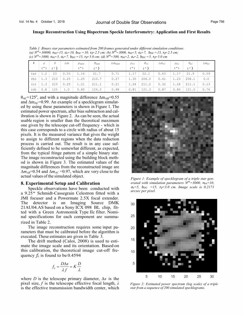
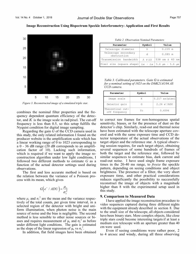
θAC=125o, and with a magnitude difference ΔmAB=0.55 and ΔmAC=0.99. An example of a specklegram simulat-ed by using these parameters is shown in Figure 1. The estimated power spectrum, after bias subtraction and cal-ibration is shown in Figure 2. As can be seen, the actual usable region is smaller than the theoretical maximum one given by the telescope cut-off frequency - which in this case corresponds to a circle with radius of about 15 pixels. It is the measured variance that gives the weight to assign to different regions when the data reduction process is carried out. The result is in any case suf-ficiently defined to be somewhat different, as expected, from the typical fringe pattern of a simple binary star. The image reconstructed using the building block meth-od is shown in Figure 3. The estimated values of the magnitude differences from the reconstructed image are ∆mAB=0.54 and ∆mAC =0.97, which are very close to the actual values of the simulated object.

8. Experimental Setup and Calibration

. The image reconstruction requires some input pa-

rameters that must be calibrated before the algorithm is executed. These estimates are given in Table 3.

where D is the telescope primary diameter,

# ρPS θPS ρBS

1.2 23 0.55 1.16 21.7 0.71 1.17 22.1 0.63 1.17 21.9 0.59

1.3 210 0.25 1.25 210.7 0.27 1.30 206.0 0.41 1.23 208.1 0.0

1.3 210 0.25 1.21 211.1 0.21 1.26 211.2 0.32 1.26 211.1 0.13

0.8 125 1.0 0.80 124.2 0.98 0.81 121.3 0.87 0.80 121.5 0.76

Table 1. Binary star parameters estimated from 200 frames generated under different simulation conditions:

(a) Nph=30000, nth=15, σe=10, bDC =10, r0=2.5 cm; (b) Nph=3000, nth=5, σe=7, bDC =15, r0=2.5 cm;

(c) Nph=1000, nth=5, σe=7, bDC =15, r0=5.0 cm; (d) Nph=500, nth=2, σe=2, bDC =5, r0=5.0 cm

Figure 2: Estimated power spectrum (log scale) of a triple star from a sequence of 200 simulated specklegrams.

c

D x Df K

f

= =



where μc and σc2 are the mean and the variance respec-

tively of the total counts, per given

and requires measurement of μc and σc2 as before

under different light conditions. The gain is estimated as the slope of the linear regression of μc vs σc

2.

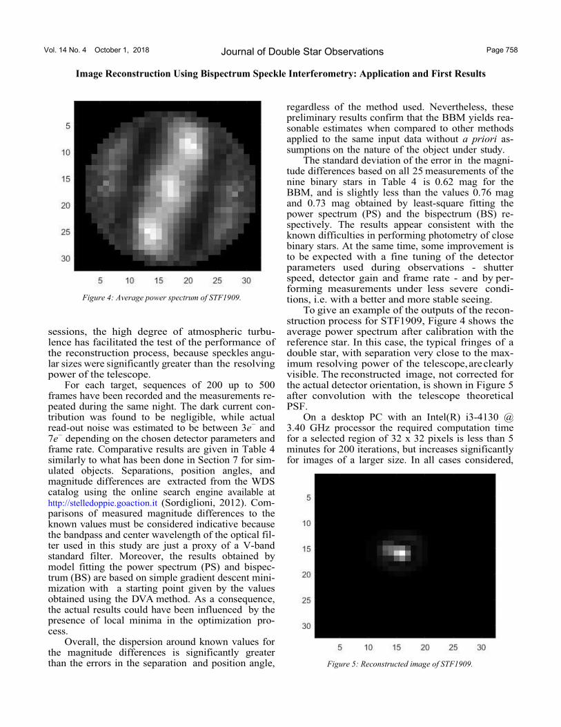
9. Comparison to Measured Data I have applied the image reconstruction procedure to

video sequences captured during three different nights with the equipment already described in section 8. Due to the small size of the telescope, all objects considered have been binary stars. More complex objects, like close triple stars could become interesting targets if at least a medium size telescope with an aperture greater than 40 cm were used.

Figure 3. Reconstructed image of a simulated triple star.

( ) 2/ c

c

G e ADU

− =

Parameter

Pixel size (square shape) 5.6 µm · 5.6 µm

Table 2. Observation Nominal Parameters

Parameter Symbol Value

Image scale K 0.217 as/pixel

Detector gain G 2.26 e-/ADU

Theoretical cut-

off frequency fc 0.4594

Table 3. Calibrated parameters. Gain G is estimated for a nominal setting of 1023 on the DMK21AU04.AS CCD camera.



engine available at http://stelledoppie.

Figure 4: Average power spectrum of STF1909.

Figure 5: Reconstructed image of STF1909.

http://stelledoppie/



tion can be stopped once the rate of decrease of dk reduces significantly.

10. Conclusions

11. Acknowledgements The author wishes to thank Carlo Perotti for his

support during observations and Karl-Ludwig Bath for useful discussions in the early stages of this work. This research has made use of Cartes du Ciel, the Washing-ton Double Star Catalog, and the double star database Stelle Doppie.

12. References

Caloi, R. M., 2008, Journal of Double Star Observa-tions, 4-3, 111-118.

Genet, R. M., 2015, Journal of Double Star Observa-tions, 11-1S, 266-276.

Astron. Astrophys., 541, A46.

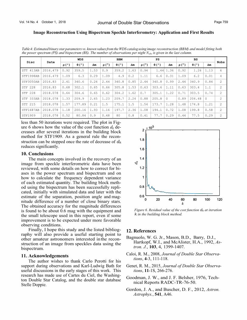
Table 4: Estimated binary star parameters vs. known values from the WDS catalog using image reconstruction (BBM) and model fitting both the power spectrum (PS) and bispectrum (BS). The number of observations per night Nobs is given in the last column.

Figure 6. Residual value of the cost function dk

Disc Date WDS BBM PS BS

Nobs ρ(") θ(º) Δm ρ(") θ(º) Δm ρ(") θ(º) Δm ρ(") θ(º) Δm

STT 413AB 2016.479 0.92 359.5 1.53 0.9 359.2 1.63 0.94 1.44 1.36 0.92 1.26 1.13 6

STF1998AB 2016.479 1.09 6.3 0.29 1.09 4.9 0.2 1.11 6.6 0.31 1.09 6.2 0.01 4

STF3050AB 2016.83 2.41 340.6 0.26 2.44 340.8 0.85 2.44 340.8 0.99 2.44 340.9 0.84 2

STF 228 2016.83 0.68 302.1 0.65 0.66 305.8 1.53 0.63 303.6 1.11 0.63 303.4 1.1 2

STF 228 2018.078 0.64 304.6 0.65 0.62 304.2 1.62 0.7 305.1 1.22 0.71 303.5 0.74 2

STF 333AB 2018.078 1.33 209.9 2.65 1.23 209.7 2.24 0.88 205.8 0 0.89 204.48 0 2

STT 215 2018.078 1.57 177.89 0.21 1.5 175.1 1.5 1.54 173.7 1.28 1.48 174.8 1.21 2

STF1687AB 2018.078 1.18 200.16 1.93 1.16 197.7 2.36 1.08 194.1 0.72 1.08 199.8 0.58 2

STF1909 2018.078 0.52 80.84 0.9 0.48 80 0.8 0.41 77.7 0.29 0.44 77.5 0.29 2



Astron. As-trophys., 278, 328.

Labeyrie, A., 1970, Astron. Astrophys., 6, 85.

McGlamery, B. L., 1976, Proc. SPIE 0074 Image Pro-cessing.

Stelle Dop-pie, 2.

2017, Soc. Am. A, 34, 6.

Weigelt, G., 1977, Opt. Commun., 21, 55.

Wirnitzer, B., 1985, J. Opt. Soc. Am. A, 2,14.

Documents

Image Reconstruction Using Bispectrum Speckle ... · Roberto Maria Caloi [email protected] Abstract: Vol. 14 No. 4 October 1, 2018 Journal of Double Star Observations Page 751 ... By