Embed Size (px)
Citation preview
Lecture 11Image Processing
Erdal Yılmaz
July 29, 2013
Lecture 11 Image Processing

Before we begin
HW3 solutions
HW4 will be assigned today
PR Projects
Lecture 11 Image Processing

Today is Lena Day
Colors, RGB
Image files
MATLAB Demos
Lecture 11 Image Processing

Pixel and Bitmaps
Pixel = Picture Element
Bitmaps store color information of pixels
Lecture 11 Image Processing
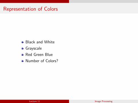
Representation of Colors
Black and White
Grayscale
Red Green Blue
Number of Colors?
Lecture 11 Image Processing

Anatomy of Files
Text Files vs. Binary Files
Example Text files:
.txt (plain), .html (markup)
Example Binary files:
.exe .bmp .png .zip
Lecture 11 Image Processing

X-raying Binary Files
Use hexdump
File formats
File headers
Lecture 11 Image Processing
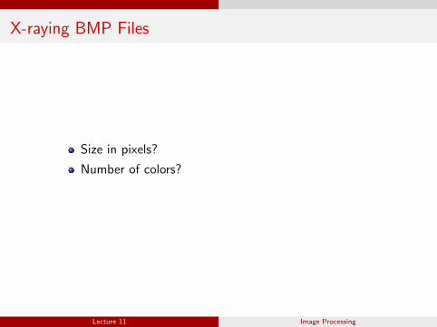
X-raying BMP Files
Size in pixels?
Number of colors?
Lecture 11 Image Processing

MATLAB Image Formats
imformats
shows information about the image formats MATLAB canwork on
imfinfo
shows information related to an image file
Lecture 11 Image Processing

Reading Image Files
imread
reads an image file and returns image data in an array
Usage
% A = imread(FILENAME, FORMAT)
data = imread('lena.png','png');
Lecture 11 Image Processing

Displaying Image Data
imshow
displays the image in a figure window. if RGB layers areprovided it is displayed in colors. If a single layer is used, itwill be displayed in grayscale.
Usage
imshow('lena.png');
[x,map] = imshow('lena.tif');imshow(x,map);
I = imread('lena.png');imshow(I);
Lecture 11 Image Processing

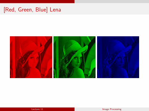
[Red, Green, Blue] Lena
l = imread('lena.png');
r = l;r(:,:,2:3) = 0;figureimshow(r)
g = l;g(:,:,1:2:3) = 0;figureimshow(g)
b = l;b(:,:,1:2) = 0;figureimshow(b)
Lecture 11 Image Processing
[Red, Green, Blue] Lena
Lecture 11 Image Processing

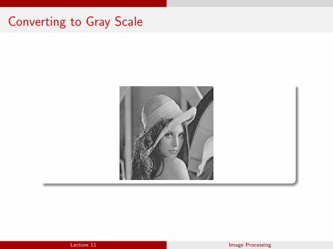
Converting to Gray Scale
togray.m
data = imread('lena.png');
size(data) % 3D array! ( 512 x 512 x 3 )
r = data(:,:,1);g = data(:,:,2);b = data(:,:,3);
gray = (r/3+g/3+b/3);
data(:,:,1) = gray;data(:,:,2) = gray;data(:,:,3) = gray;
imshow(data)
Lecture 11 Image Processing
Converting to Gray Scale
Lecture 11 Image Processing

Writing Image Files
imwrite
writes the image to a file
Usage
% imwrite(A, FILENAME, FORMAT)
imwrite(data, 'lena gray.png', 'png');
Lecture 11 Image Processing

Filtering
We will apply a 3x3 matrix which is called a filter toprocess the image.
Averaging and Blurring
Fa =
1 1 11 1 11 1 1
/9 Fb =
0 1 01 1 10 1 0
/5
Lecture 11 Image Processing

Applying the Filter
function pdata = filter lena(fname, fmt, F)data = imread([fname,'.',fmt], fmt);[n m c] = size(data);pdata = zeros(n,m,c);ddata = double(data); %convert from uint8 to double% ignoring a thin frame around the picturefor i = 2:n−1 % move to the next rowfor j = 2:m−1 % move to the next columnfor k = 1:3 % apply the filter to all 3 layerspdata(i,j,k) = ...
sum(sum(F .* ddata(i−1:i+1, j−1:j+1, k)));end
endendpdata = uint8(floor(pdata)); %convert back to uint8imwrite(pdata, [fname,' filtered.',fmt], fmt);
Lecture 11 Image Processing
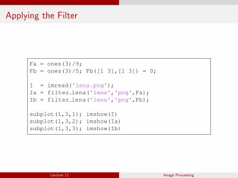
Applying the Filter
Fa = ones(3)/9;Fb = ones(3)/5; Fb([1 3],[1 3]) = 0;
I = imread('lena.png');Ia = filter lena('lena','png',Fa);Ib = filter lena('lena','png',Fb);
subplot(1,3,1); imshow(I)subplot(1,3,2); imshow(Ia)subplot(1,3,3); imshow(Ib)
Lecture 11 Image Processing

Blurred Images
Lecture 11 Image Processing
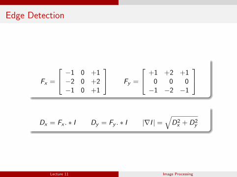
Edge Detection
Fx =
−1 0 +1−2 0 +2−1 0 +1
Fy =
+1 +2 +10 0 0−1 −2 −1
Dx = Fx . ∗ I Dy = Fy . ∗ I |∇I | =√
D2x + D2
y
Lecture 11 Image Processing
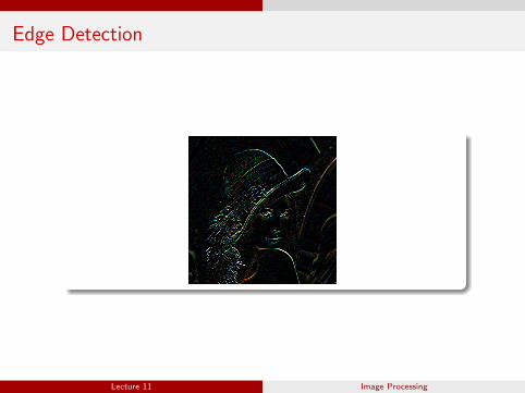
Edge Detection
Lecture 11 Image Processing