University of Texas at Austin CS384G - Computer Graphics Fall 2008 Don Fussell

Image processing

University of Texas at Austin CS384G - Computer Graphics Fall 2008 Don Fussell 2

Reading

Jain, Kasturi, Schunck, Machine Vision. McGraw-Hill, 1995. Sections 4.2-4.4, 4.5(intro), 4.5.5, 4.5.6, 5.1-5.4.

University of Texas at Austin CS384G - Computer Graphics Fall 2008 Don Fussell 3

Image processing

An image processing operation typically defines a new image g in terms of an existing image f.

The simplest operations are those that transform each pixel in isolation. These pixel-to-pixel operations can be written:

Examples: threshold, RGB grayscale

Note: a typical choice for mapping to grayscale is to apply the YIQ television matrix and keep the Y.€

g(x,y) = t( f (x,y))

€

Y

I

Q

⎡

⎣

⎢ ⎢ ⎢

⎤

⎦

⎥ ⎥ ⎥=

0.299 0.587 0.114

0.596 −0.275 −0.321

0.212 −0.523 0.311

⎡

⎣

⎢ ⎢ ⎢

⎤

⎦

⎥ ⎥ ⎥

R

G

B

⎡

⎣

⎢ ⎢ ⎢

⎤

⎦

⎥ ⎥ ⎥

University of Texas at Austin CS384G - Computer Graphics Fall 2008 Don Fussell 4

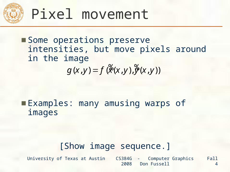
Pixel movement

Some operations preserve intensities, but move pixels around in the image

Examples: many amusing warps of images

[Show image sequence.]

% %( , ) ( ( , ), ( , ))g x y f x x y y x y=

University of Texas at Austin CS384G - Computer Graphics Fall 2008 Don Fussell 5

Noise Image processing is also useful for noise reduction and edge

enhancement. We will focus on these applications for the remainder of the lecture…

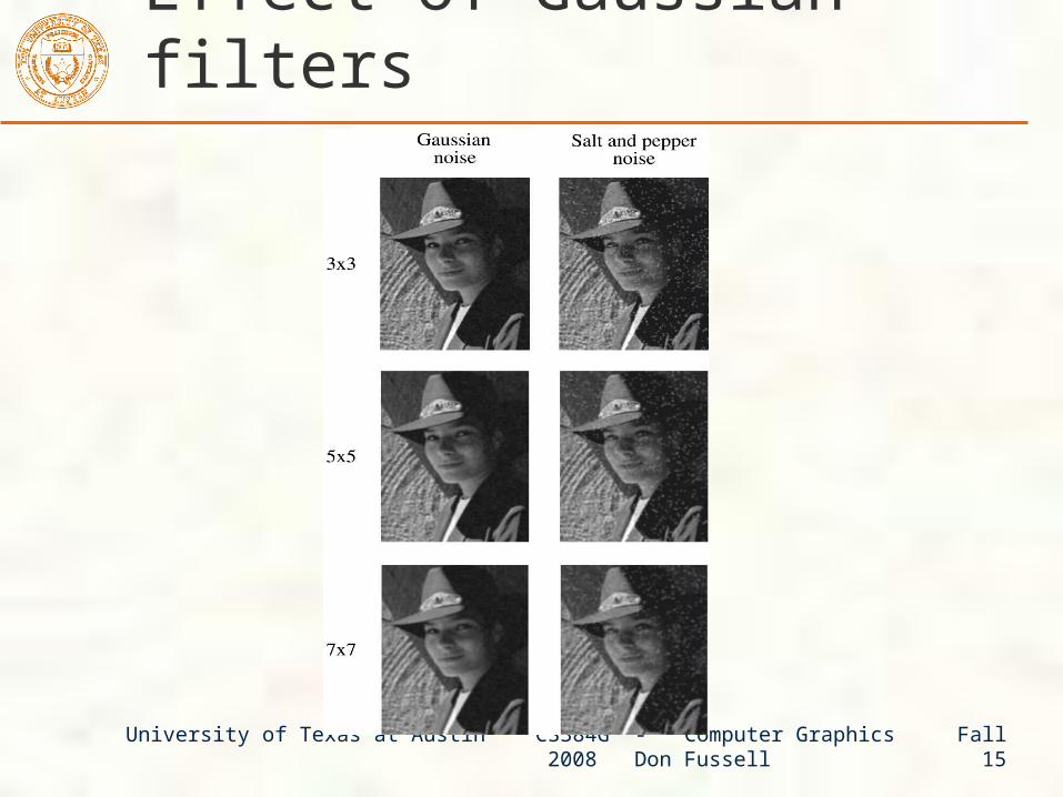
Common types of noise: Salt and pepper noise:

contains random occurrences of black and white pixels

Impulse noise: contains random occurrences of white pixels

Gaussian noise: variations in intensity drawn from a Gaussian normal distribution

University of Texas at Austin CS384G - Computer Graphics Fall 2008 Don Fussell 6

Ideal noise reduction

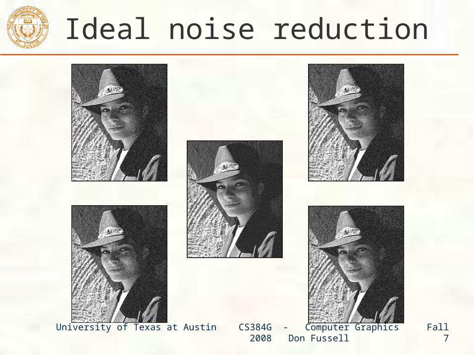
University of Texas at Austin CS384G - Computer Graphics Fall 2008 Don Fussell 7

Ideal noise reduction

University of Texas at Austin CS384G - Computer Graphics Fall 2008 Don Fussell 8

Practical noise reduction

How can we “smooth” away noise in a single image?

Is there a more abstract way to represent this sort of operation? Of course there is!

University of Texas at Austin CS384G - Computer Graphics Fall 2008 Don Fussell 9

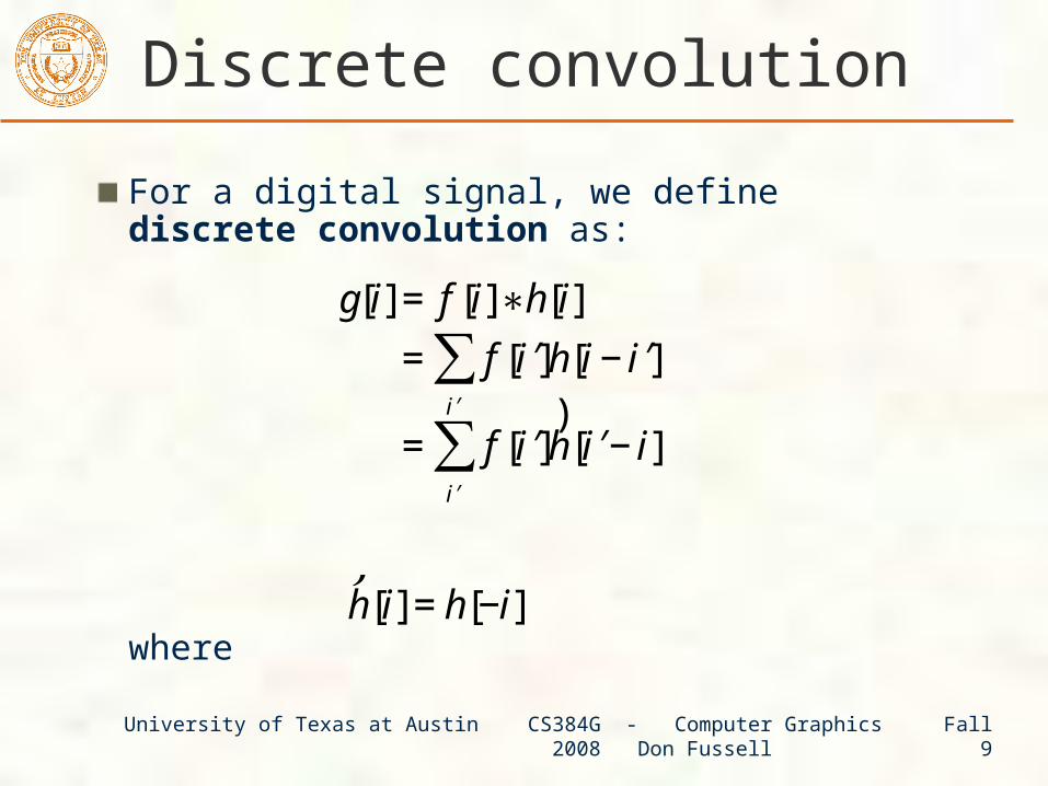
Discrete convolution

For a digital signal, we define discrete convolution as:

where

€

g[i] = f [i]∗h[i]

= f [ ′ i ]h[i − ′ i ]′ i

∑= f [ ′ i ]

) h [ ′ i − i]

′ i

∑

€

) h [i] = h[−i]

University of Texas at Austin CS384G - Computer Graphics Fall 2008 Don Fussell 10

Discrete convolution in 2D

Similarly, discrete convolution in 2D becomes:

where

€

g[i, j] = f [i, j]∗h[i, j]

= f [ ′ i , ′ j ]h[i − ′ i , j − ′ j ]′ j

∑′ i

∑

= f [ ′ i , ′ j ]) h [ ′ i − i, ′ j − j]

′ j

∑′ i

∑

€

) h [i, j] = h[−i,− j]

University of Texas at Austin CS384G - Computer Graphics Fall 2008 Don Fussell 11

Convolution representation

Since f and h are defined over finite regions, we can write them out in two-dimensional arrays:

Note: This is not matrix multiplication!Q: What happens at the edges?

University of Texas at Austin CS384G - Computer Graphics Fall 2008 Don Fussell 12

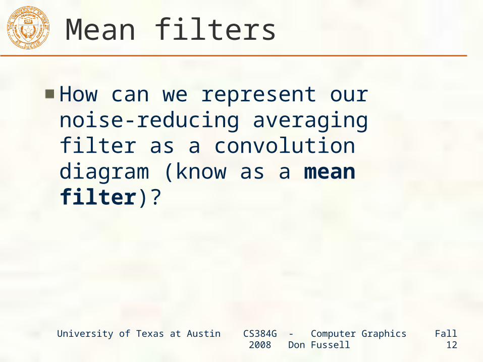
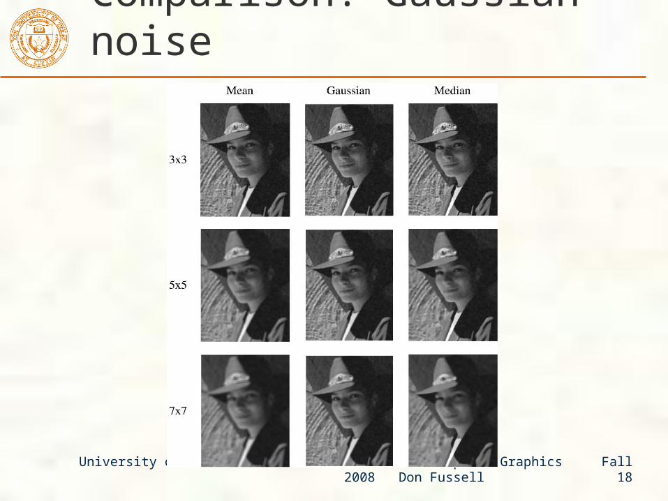
Mean filters

How can we represent our noise-reducing averaging filter as a convolution diagram (know as a mean filter)?

University of Texas at Austin CS384G - Computer Graphics Fall 2008 Don Fussell 13

Effect of mean filters

University of Texas at Austin CS384G - Computer Graphics Fall 2008 Don Fussell 14

Gaussian filters

Gaussian filters weigh pixels based on their distance from the center of the convolution filter. In particular:

This does a decent job of blurring noise while preserving features of the image.What parameter controls the width of the Gaussian? What happens to the image as the Gaussian filter kernel gets wider?What is the constant C? What should we set it to?

2 2 2( ) /(2 )

[ , ]i je

h i jC

σ− +

=

University of Texas at Austin CS384G - Computer Graphics Fall 2008 Don Fussell 15

Effect of Gaussian filters

University of Texas at Austin CS384G - Computer Graphics Fall 2008 Don Fussell 16

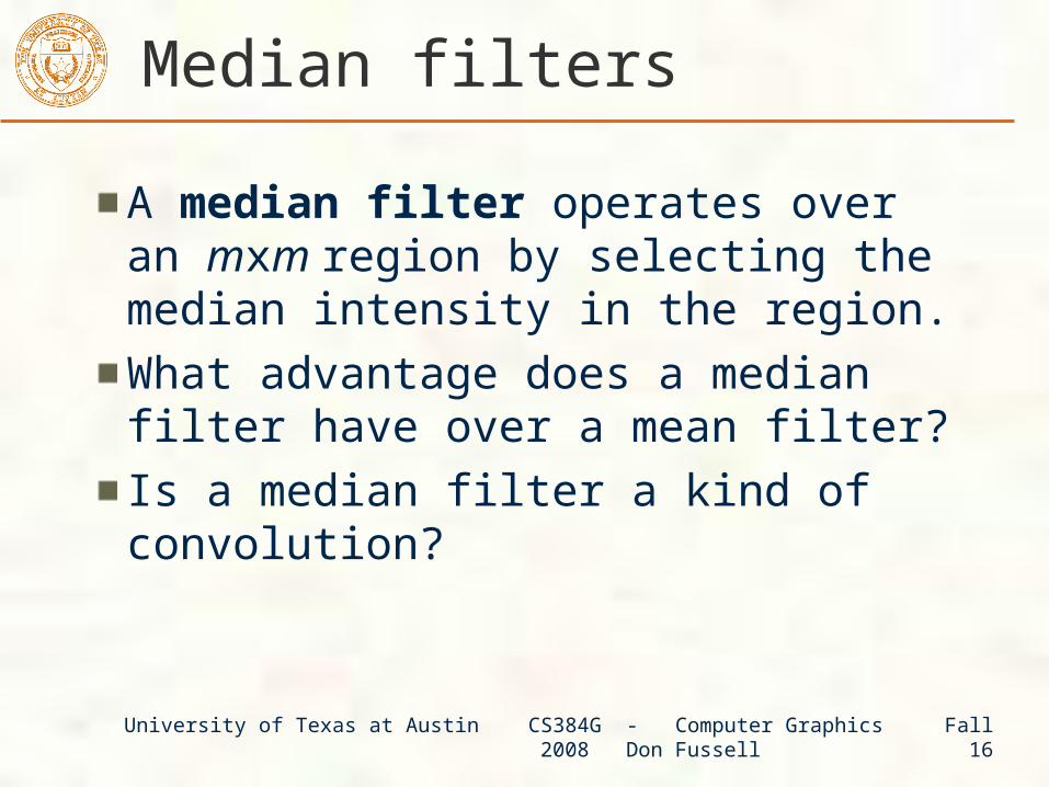
Median filters

A median filter operates over an mxm region by selecting the median intensity in the region.

What advantage does a median filter have over a mean filter?

Is a median filter a kind of convolution?

University of Texas at Austin CS384G - Computer Graphics Fall 2008 Don Fussell 17

Effect of median filters

University of Texas at Austin CS384G - Computer Graphics Fall 2008 Don Fussell 18

Comparison: Gaussian noise

University of Texas at Austin CS384G - Computer Graphics Fall 2008 Don Fussell 19

Comparison: salt and pepper noise

University of Texas at Austin CS384G - Computer Graphics Fall 2008 Don Fussell 20

Edge detection

One of the most important uses of image processing is edge detection:

Really easy for humans

Really difficult for computers

Fundamental in computer vision

Important in many graphics applications

University of Texas at Austin CS384G - Computer Graphics Fall 2008 Don Fussell 21

What is an edge?

Q: How might you detect an edge in 1D?

University of Texas at Austin CS384G - Computer Graphics Fall 2008 Don Fussell 22

Gradients

The gradient is the 2D equivalent of the derivative:

Properties of the gradientIt’s a vectorPoints in the direction of maximum increase of fMagnitude is rate of increase

How can we approximate the gradient in a discrete image?

( , ) ,f f

f x yx y

⎛ ⎞∂ ∂∇ =⎜ ⎟⎝∂ ∂ ⎠

University of Texas at Austin CS384G - Computer Graphics Fall 2008 Don Fussell 23

Less than ideal edges

University of Texas at Austin CS384G - Computer Graphics Fall 2008 Don Fussell 24

Steps in edge detection

Edge detection algorithms typically proceed in three or four steps:

Filtering: cut down on noiseEnhancement: amplify the difference between edges and non-edgesDetection: use a threshold operationLocalization (optional): estimate geometry of edges beyond pixels

University of Texas at Austin CS384G - Computer Graphics Fall 2008 Don Fussell 25

Edge enhancement

A popular gradient magnitude computation is the Sobel operator:

We can then compute the magnitude of the vector (sx, sy).

1 0 1

2 0 2

1 0 1

1 2 1

0 0 0

1 2 1

x

y

s

s

−⎡ ⎤⎢ ⎥= −⎢ ⎥⎢ ⎥−⎣ ⎦

⎡ ⎤⎢ ⎥=⎢ ⎥⎢ ⎥− − −⎣ ⎦

University of Texas at Austin CS384G - Computer Graphics Fall 2008 Don Fussell 26

Results of Sobel edge detection

University of Texas at Austin CS384G - Computer Graphics Fall 2008 Don Fussell 27

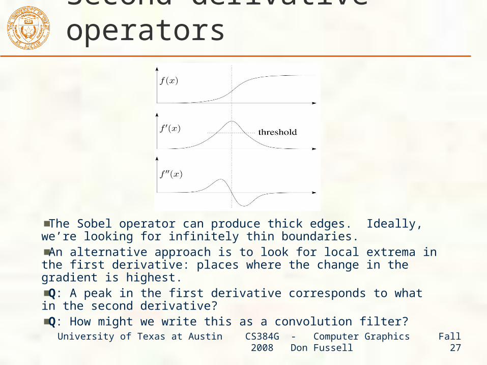
Second derivative operators

The Sobel operator can produce thick edges. Ideally, we’re looking for infinitely thin boundaries.

An alternative approach is to look for local extrema in the first derivative: places where the change in the gradient is highest.

Q: A peak in the first derivative corresponds to what in the second derivative?

Q: How might we write this as a convolution filter?

University of Texas at Austin CS384G - Computer Graphics Fall 2008 Don Fussell 28

Localization with the Laplacian

An equivalent measure of the second derivative in 2D is the Laplacian:

Using the same arguments we used to compute the gradient filters, we can derive a Laplacian filter to be:

Zero crossings of this filter correspond to positions of maximum gradient. These zero crossings can be used to localize edges.

2 22

2 2( , )f f

f x yx y

∂ ∂∇ = +

∂ ∂

2

0 1 0

1 4 1

0 1 0

⎡ ⎤⎢ ⎥Δ = −⎢ ⎥⎢ ⎥⎣ ⎦

University of Texas at Austin CS384G - Computer Graphics Fall 2008 Don Fussell 29

Localization with the Laplacian

Original Smoothed

Laplacian (+128)

University of Texas at Austin CS384G - Computer Graphics Fall 2008 Don Fussell 30

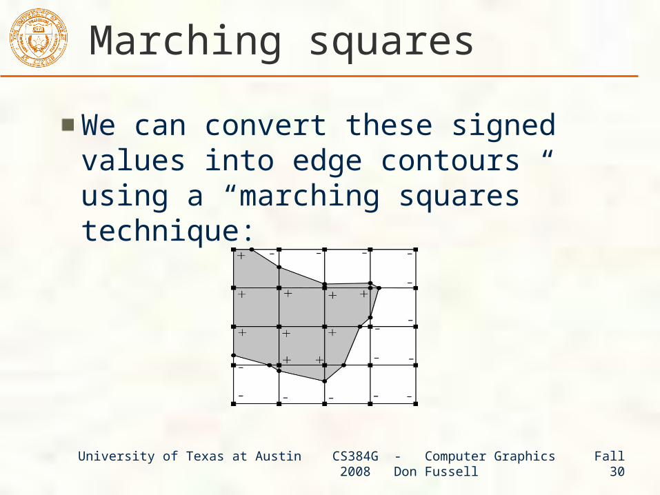
Marching squares

We can convert these signed values into edge contours using a “marching squares” technique:

University of Texas at Austin CS384G - Computer Graphics Fall 2008 Don Fussell 31

Sharpening with the Laplacian

Original Laplacian (+128)

Original + Laplacian Original - Laplacian

Why does the sign make a difference?How can you write each filter that makes each bottom image?

University of Texas at Austin CS384G - Computer Graphics Fall 2008 Don Fussell 32

Spectral impact of sharpeningWe can look at the impact of sharpening on the Fourier spectrum:

2

0 1 0

1 5 1

0 1 0

δ−⎡ ⎤

⎢ ⎥−Δ = − −⎢ ⎥⎢ ⎥−⎣ ⎦

Spatial domain Frequency domain

University of Texas at Austin CS384G - Computer Graphics Fall 2008 Don Fussell 33

Summary

What you should take away from this lecture:The meanings of all the boldfaced terms.

How noise reduction is done

How discrete convolution filtering works

The effect of mean, Gaussian, and median filters

What an image gradient is and how it can be computed

How edge detection is done

What the Laplacian image is and how it is used in either edge detection or image sharpening

University of Texas at Austin CS384G - Computer Graphics Fall 2008 Don Fussell 34

Next time: Affine Transformations

Topic:How do we represent the rotations, translations,

etc. needed to build a complex scene from simpler objects?Read:

• Watt, Section 1.1.

Optional:• Foley, et al, Chapter 5.1-5.5.• David F. Rogers and J. Alan Adams,

Mathematical Elements for Computer Graphics, 2nd Ed., McGraw-Hill, New York, 1990, Chapter 2.