Image Noise John Morris Department of Computer Science, Tamaki Campus The University of Auckland

Image NoiseImage Noise

John Morris

Department of Computer Science, Tamaki CampusThe University of Auckland

2

Stereo Image Noise Sources Stereo Image Noise Sources • Signal noise

• Electromagnetic interference eg cross-talk • Quantum behaviour of electronic devices

eg resistor shot-noise• Quantization: digitization of real-valued signals

• Geometric sources• Discrete pixel sensors with finite area• Occlusions• Perspective distortion

• Opto-Electronic sources• Sensitivity variations between cameras• Different ‘dark noise’ levels• Real lenses• Depth-of-focus

• Optical Surface properties

Single camera sources Stereo (2-camera) sources

Note that we use the term ‘noise’ for all problem sources!

3

Stereo Image Noise SourcesStereo Image Noise Sources

Optical Surface Properties Lambertian scatterers

A “perfect” scatterer scatters light uniformly in all directions

Most correspondence algorithms assume perfect (Lambertian) scatterers This means that surface patches will appear with the same intensity –

independent of viewing angle .. Simple matching

• Intensities should be the same (perturbed by random noise!)

Reflectors

4

Stereo Image Noise SourcesStereo Image Noise Sources

Ordering Constraint Often used to simplify matching algorithms

Particularly dynamic programming

Imaged points appear in the same order in both images Violated by ‘poles’ – narrow objects in front of planes

5

Electronic NoiseElectronic Noise

Antennae (Receivers) Wires act as antennae for EM waves ‘Wire’ includes discrete wires

but also Tracks on circuit boards Interconnects on chips

Transmitters Any wire with a changing current emits EM waves

6


Digital circuits very rapid transitions (switching events) High frequency signals

Crosstalk One wire is influenced by neighbouring wires

Ideal digital signal

‘Instaneous’ rise or fall≡ infinite frequency perfect radiator

Real digital signal

‘Fast’ rise or fall high frequency very good radiator

Signal driven into purple wire

Signal picked up on green wire

EM coupling

7

Electronic noiseElectronic noise

Quantum effects Resistor ‘shot’ noise

Resistive element is composed of discrete atoms Always in motion for all T > 0oK (absolute zero) Noise as effective resistance changes Moving atoms ‘collide’ with electrons moving to form the

current Random fluctuations in current

or

Noise as effective resistance changes Similar effects in all current carrying or producing devices

• Transistors• Capacitors• Inductors, etc

e-

e-

8

Electronic noiseElectronic noise

Digitization noise Analogue signal

Taking all possible values• At least at a macroscopic level!

Digital signal Represented by a range of integers

• 0 .. 255 (8 bit signal)• 0 .. 4095 (12 bit signal)• -2048 .. 2047 (12 bit signed signal)

A to D converter Decides to which integer value to map a real value

Discretization Values which differed (in real domain) become the same (in integer domain)

9

Opto-electronic noiseOpto-electronic noise

Cameras have different gain settings Amplifiers are not ‘matched’ perfectly

Sensors have different ‘dark current’ characteristics All sensors produce some electrons (current) with no light Quantum ‘tunneling’ out of the sensor device

Stereo Problem

Light Intensity

Cu

rren

t Different slopesGains differ

Different offsetsDark currents differ

10


Summary

11

Geometric noiseGeometric noise

‘Pixelisation’ of images Sensor is divided into discrete regions – pixels ‘Edges’ in images don’t conveniently fall onto pixel

boundaries

Red object

Blue object Real image

has blurrededges

12

Geometric noiseGeometric noise

Occlusions Points visible from one camera onlyPoints which it is impossible to match

Perspective distortion Field of view in one camera differs from

other Left and right images contain different

numbers of pixels Impossible to match all pixels correctly

Stereo Problem

B

ML

B

MR

13

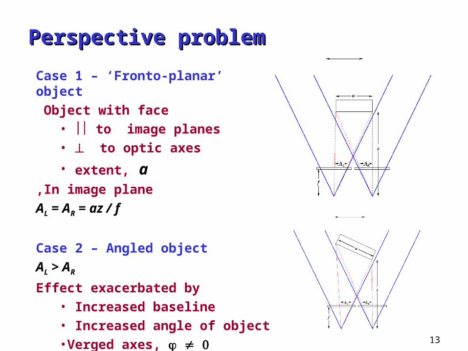
Perspective problemPerspective problem

Case 1 – ‘Fronto-planar’ object

Object with face • to image planes• to optic axes

• extent, aIn image plane,

AL = AR = az / f

Case 2 – Angled object

AL > AR

Effect exacerbated by• Increased baseline• Increased angle of object•Verged axes,

14

Optical effectsOptical effects

Real lenses Finite depth of field

Image is ‘in focus’ over finite region only• Due to deviations of real (thick) lens from

ideal shape Depth of field increased by decreasing

aperture• Always work with a small aperture!• f-stop

• Ratio of focal length to aperture• ‘f-stop’ = f / a• ‘f’ = 1.4 – aperture wide open

• f’ = 22 – aperture closed down

a

f

Mechanicalaperture

Imageplane

Real lens

For accurate work (objects in focus over a wide range)Use more light to permit narrower aperture

15

Optical effectsOptical effects

Depth of focus Finite depth of field

Image is ‘in focus’ over finite region only• Due to deviations of real (thick) lens from

ideal shape Depth of field increased by decreasing

aperture• Always work with a small aperture!• f-stop

• Ratio of focal length to aperture• ‘f-stop’ = f / a• ‘f’ = 1.4 – aperture wide open

• f’ = 22 – aperture closed down

a

f=22

Mechanicalaperture

Imageplane

Real lens

For accurate work (objects in focus over a wide range)Use more light to permit narrower aperture

f=1.4

Depth of field

16

Lambertian ScatterersLambertian Scatterers

‘Perfect scattering’ Intensity of scattered light is the

same in all directionsObservers at all angles see the

same intensity

Characteristics of a scattering surface Optically ‘rough’ Surface roughness ≈ = wavelength of incident light 700-400 nm for visible light

17

ReflectorsReflectors

Perfect reflector 100% of incident intensity reflected Angle of incidence = angle of

reflection i = r

All reflected intensity seen at one angle

Properties of a reflecting surface Optically smooth Surface roughness

irir

18

Smooth surface

Real SurfacesReal Surfaces

Reflector Most of incident intensity reflected Bright ‘spot’ seen over a small angle

Properties of a reflecting surface Optically smooth Surface roughness

Specular reflections are the result of partly reflecting surfaces Water surfaces Polished glass, plastic, …

ir

19


Scattering surface Reasonably uniform distribution of intensity

with angle Intensity of the same patch varies with angle Intensity mis-match between L and R images Systematic mis-match between views of the

same patch One is always less intense than the other

Shape of reflectance curve varies with surfaces

Random mis-match between different patches

Reflectance curves can be dependent also Different views of the same patch appear to

have different colours

20


Grating effects In extreme cases

Regular surface variations with dimensions

Grating effects Spectrum generation Small variations in view angle

large colour variations

Systematic mis-match between different patches

21

Ordering constraintOrdering constraint

If M appears to the left of N in the left image,it should appear to the left of N in the right image Violated by ‘poles’

22

Stereo Correspondence is an ill-posed problem!Stereo Correspondence is an ill-posed problem!

There are always multiple solutions!There are always multiple solutions!

oror

23

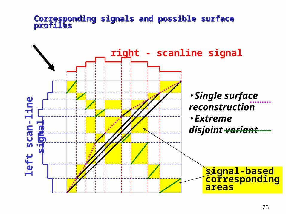
right - scanline signal

left

scan

-line

sig

nal

signal-basedcorrespondingareas

Corresponding signals and possible surface profilesCorresponding signals and possible surface profiles

•Single surface reconstruction•Extreme disjoint variant

24

Effect of NoiseEffect of Noise

but …

What happens if we use ‘noise-free’ images?

L Image - ‘corridor’ setSynthetic (ray traced)

Precise ‘ground truth’is available

25

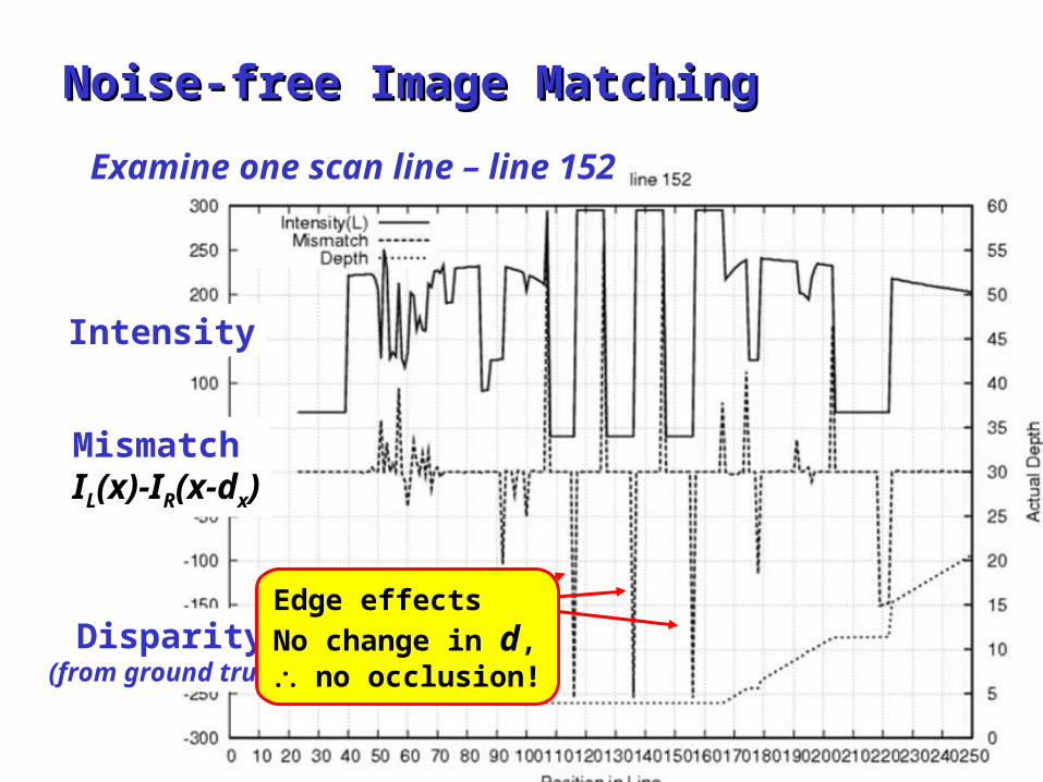
Noise-free Image MatchingNoise-free Image Matching

MismatchIL(x)-IR(x-dx)

Intensity

Disparity(from ground truth)

Examine one scan line – line 152Mismatch is the matching error

R image pixels shifted by known d(from ground truth)Zero difference with L pixel?Even ‘noise-free’ images have matching errors!

26

Real Image MatchingReal Image Matching


Intensity


Tsukuba – line 173

Occlusion

?

27

Noise-free Image MatchingNoise-free Image Matching


Intensity


Examine one scan line – line 152

Edge effects

No change in d, no occlusion!

28

Distribution of signal differences

Pixel-wise correspondences – ‘Tsukuba’ pair (line 173)Pixel-wise correspondences – ‘Tsukuba’ pair (line 173)

Grey-codedsignal differences

29

Matching in the presence of noiseMatching in the presence of noise

Correlation algorithms Match over a window Correlation functions: SSD (sum squared differences), SAD (sum absolute differences)

Average matching errors Handles random intensity fluctuations

• Electronic, quantization, … noise Doesn’t handle

• Occlusions• Pixelisation

• Intensity anomalies in one window compared to the other• Gain and dark noise variations• Perspective

• Tries to assign all pixels in a window to the same disparity• Non-Lambertian surfaces & specular effects

Normalised correlation functions Normalize pixel intensities to mean within a window

Some tolerance for gain and dark noise changes• Often not worth the additional computational effort!• Better: Correct the images at source!

• Align amplifiers, calibrate electronics, …

30

Correlation algorithmsCorrelation algorithms

Generally poor matching Mismatches (small windows) or Blurred edges due to large windows

Simple (almost trivial!) codeAdaptive windows improve performance

31

Correlation-Based MethodsCorrelation-Based Methods Matching Performance

The success of correlation-based methods depends on whether the image window in one image exhibits a distinctive structure that occurs infrequently in the search region of the other image.

How to choose the size of the window, wh? Too small a window

• may not capture enough image structure and • may be too noise sensitive many false matches

Too large a window • makes matching less sensitive to noise (desired) but also• decreases precision

(blurs disparity map)

An adaptive searching window has been proposed

32

Correlation MethodsCorrelation Methods

Input – Ground truth

3x3 windowToo noisy!

7x7 windowSharp edges are blurred!

Adaptive windowSharp edges and less noise

33

Correlation-Based MethodsCorrelation-Based Methods

34


Generally poor matching Mismatches (small windows) or Blurred edges due to large windows

Simple (almost trivial!) codefor each pixel position,w

for each disparity, d

Cwd = (ILw+j-IR

w+j-d)2

Choose min(Cwd) over d d for position w

Fast enough?

35


Not fast enough for small images For nn image, d disparity values and hw window – O (n2dhw) For small (300x300) images and low depth accuracy (5% d = 20 ) If n = 3x102, d = 20, h=w=9, then t(n) = c 81 2 x 10 9 x 104 ≈

1.5 x 107 For a 3GHz processor, cycles / pixel ≈ 3 109 / 1.5 x 107 ≈ 200 ??? Enough to

Compute indices, Fetch two pixels, Subtract Square or absolute difference Find minimum from d costs Repeat for adaptive window?

but ……

36


Moderate resolution images For moderate (1Mpixel) images and reasonable depth accuracy (1% d

= 100 ) If n = 103, d = 100, h=w=9, then t(n) = c 81 102 106 ≈ 1010 For a 3GHz processor, cycles / pixel ≈ 3 109 / 1010 ≈ 0.3 Inherently parallel Cwd(IL

w+j-IRw+j-d)2

Hardware acceleration needed!! MMX (Intel Graphics Processing Extensions) helps

Optimized for simple arithmetic on pixelsbut MMX pipeline needs to be filled efficiently Max 16 operations in parallel Excellent for 4 4 windows Usually 9 9 needed!

37


Easy to implement in hardware Match for each disparity at the same time Add minimum circuit Simple circuit ..

But O (hw) computations for each disparityRelatively large

38

SAD SAD Algorithm Algorithm

Block Block DiagramDiagramNote:Note:High ‘fan-in’ for High ‘fan-in’ for SAD calculator SAD calculator blockblockStrains FPGA Strains FPGA routing resourcesrouting resourcesLarge buffers Large buffers needed for needed for scanlinesscanlinesConsequence of Consequence of window sizewindow size

39

Correlation methodsCorrelation methods

Simplest code Poorest performance

Adaptive windows don’t help much!

Medium speed Window size is an important factor

Simple hardware realizationbut Expensive in resource use

Handle random noise only Window is just treated as vector of pixels No spatial information used Occlusions ignored

40

Dynamic Programming StereoDynamic Programming Stereo

Attempts to find the ‘best path’ (sequence of disparity values) Can recognize occlusions! Averages noise over a scanline Essentially local

Always moves ‘forward’ in a scanline Solution generated by backtracking through predecessor array

• Doesn’t adjust values in backtrack Uses the ordering constraint Readily adapted to

allow for gain and offset changes Perspective distortion

‘Stubborn’ Incorporates a penalty for occlusions Tends to make ‘streaks’ in disparity images ..\resources\DP_Gonzalez.pdf

Can be improved by using neighbouring scan lines Requires fewer scan line buffers than correlation window

41

Dynamic Programming ResultDynamic Programming Result

Note the horizontal streaks!

It’s like a bureaucrat: once a DP algorithm ‘decides’ to adopt a disparity value – it doesn’t want to change its mind!Adding inter-scanline constraints (using a neighbouring scanline)generally improves this!

42

Dynamic Programming PerformanceDynamic Programming Performance

Better matching than correlation methods ‘Global’ along scan lines Recognizes occlusions Uses ordering constraint

Uses spatial information

Time complexity O(n2d) Faster than correlation methods in software Uses memory (typical of DP algorithms) For n=103, d=102, t = c 108

c = ~30 cycles / pixel on 3GHz machine Not enough for real time in software!

43

Real time stereoReal time stereo

Real time stereo vision Implemented Gimel’farb’s Symmetric

Dynamic Programming Stereo in FPGA hardware

Real time precise stereo vision Faster, smaller hardware circuit Real time 3D maps

1% depth accuracy with 2 scan line latency at 25 frames/sec

System block diagram: lens distortion removal,misalignment correction and depth calculator

Output is stream of depth values: a 3D movie!

44

Real time 3D data acquisitionReal time 3D data acquisition

Possible Applications Collision avoidance for robots Recognition via 3D models

Fast model acquisition• Imaging technology not scanning!

Recognition of humans without markers

Tracking objects• Recognizing orientation, alignment

Process monitoringeg Resin flow in flexible (‘bag’) moulds

Motion capture – robot training System block diagram: lens distortion removal,misalignment correction and depth calculator


45

System System Block Block DiagramDiagram

Cameras

Distortion & Alignment

DP Stereo –Forward Pass

DP Stereo –Backward Pass

46

Symmetric Dynamic Programming StereoSymmetric Dynamic Programming Stereo

Don’t try to reconstruct an ‘image’ corresponding to the left (or right) image

Turn yourself into Cyclops

.. and reconstruct a Cyclopaean view Optical centre half-way along

baseline Key advantage: Label visibility

states: MR, B, ML Disparity changes are associated

with visibility state changes

47

SDPSSDPS• Disparity Calculator Block• Small • 2 x min3• 1 x min2• 1 x abs difference• 3 x adders• Mostly 8-14 bits

• Since it’s small, it can be replicated many times

Large disparity range High depth resolution

48

FPGA Stereo SystemFPGA Stereo System

FirewireCables

FirewirePhysical

Layer ASIC

FirewireLink

Layer ASIC

FPGAAlteraStratix

Parallel Host Interface

FPGAProgCable

49

An Artificial Vision SystemAn Artificial Vision System

50

Artificial System RequirementsArtificial System Requirements

Highly Parallel Computation Calculations are not complex

but There are a lot of them in megapixel+ ( >106 ) images!

High Resolution Images Depth is calculated from the disparity

If it’s only a few pixels, then depth accuracy is low Basic equation (canonical configuration only!)

Depth, z = b f d p

Baseline Focal Length

DisparityPixel size

51


Depth resolution is critical! A cricket* player can catch a 100mm ball travelling at

100km/h

High Resolution Images NeededDisparities are large numbers of pixelsSmall depth variations can be measured

but High resolution images increase the demand for processing

power!

*Strange game played in former British coloniesin which a batsmen defends 3 small sticksin the centre of a large field against a bowler whotries to knock them down!

52


Conventional processors do not have sufficient processing power

but Moore’s Law says Wait 18 months and the power will have doubledbut The changes that give you twice the power

also give your twice as many pixels in a rowand four times as many in an image!

Specialized highly parallel hardwareis the only solution!

53

Processing Power SolutionProcessing Power Solution

54

FPGA HardwareFPGA Hardware

FPGA = Field Programmable Gate Array ‘Soft’ hardware Connections and logic functions are ‘programmed’ in much

the same way as a conventional von Neuman processor Creating a new circuit is about as difficult as writing a

programme! High order parallelism is easy

Replicate the circuit n times• As easy as writing a for loop!

55


FPGA = Field Programmable Gate Array ‘Circuit’ is stored in static RAM

cells Changed as easily as reloading

a new program

56


Why is programmability important? or Why not design a custom ASIC?

Optical systems don’t have the flexibility of a human eye Lenses fabricated from rigid materials

Not possible to make a ‘one system fits all’ system Optical configurations must be designed for each application

Field of view Resolution required Physical constraints …

Processing hardware has to be adapted to the optical configuration If we design an ASIC, it will only work for one application!!

57

Correspondence or MatchingCorrespondence or Matching

58

Stereo CorrespondenceStereo Correspondence

Can you find all the matching points in these two images?

“Of course! It’s easy!”

The best computer matching algorithms get 5% or more of the points completely wrong!…and take a long time to do it!They’re not candidates for real time systems!!

59

Stereo CorrespondenceStereo Correspondence

High performance matching algorithms are global in nature Optimize over large image regions using energy

minimization schemes Global algorithms are inherently slow

Iterate many times over small regions to find optimal solutions

60

Correspondence AlgorithmsCorrespondence Algorithms

Good matching performance, global, low speed Graph-cut, belief-propagation, …

High speed, simple, local, high parallelism, lowest performance Correlation

High speed, moderate complexity, parallel, medium performance

Dynamic programming algorithms

61

Depth AccuracyDepth Accuracy

62

Stereo ConfigurationStereo Configuration Canonical configuration – Two

cameras with parallel optical axes

Rays are drawn through each pixel in the image

Ray intersections represent points imaged onto the centre of each pixel

Points along these lineshave the same disparity

but• To obtain depth information, a point

must be seen by both cameras, ie it must be in the Common Field of View

Depthresolution

63

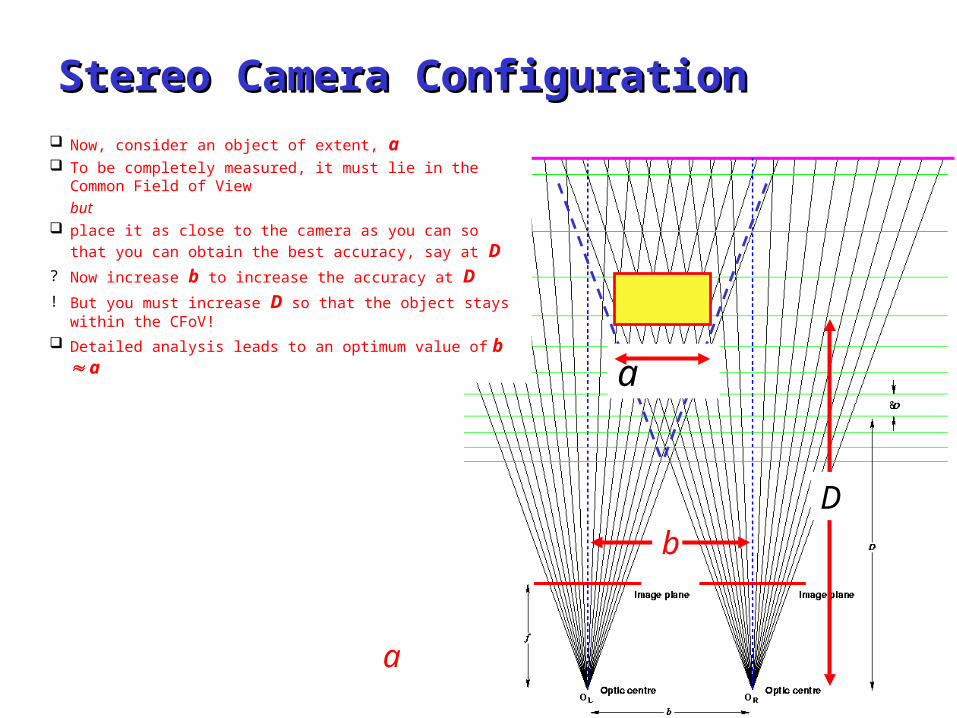
a

Stereo Camera ConfigurationStereo Camera Configuration Now, consider an object of extent, a To be completely measured, it must lie in the Common Field of View but place it as close to the camera as you can so that you can obtain the

best accuracy, say at D? Now increase b to increase the accuracy at D ! But you must increase D so that the object stays within the CFoV! Detailed analysis leads to an optimum value of b a

bD

a

64

Increasing the baselineIncreasing the baseline%

good

matc

hes

Baseline, b

Images: ‘corridor’ set (ray-traced)Matching algorithms: P2P, SAD

Increasing the baselinedecreases performance!!

65

Increasing the baselineIncreasing the baselineS

tand

ard

Devia

tion

Examine the distribution of errors

Images: ‘corridor’ set (ray-traced)Matching algorithms: P2P, SAD

Increasing the baselinedecreases performance!!

Baseline, b

66

Increased Baseline Increased Baseline Decreased Performance Decreased Performance Statistical

Higher disparity range increased probability of matching incorrectly -

you’ve simply got more choices!

Perspective Scene objects are not fronto-planar Angled to camera axes

subtend different numbers of pixels in L and R images

Scattering Perfect scattering (Lambertian) surface assumption OK at small angular differences

increasing failure at higher angles

Occlusions Number of hidden regions increases as angular difference increases

increasing number of ‘monocular’ points for which there is no 3D information!

67

EvolutionEvolutionHuman eyes ‘verge’ on an object to estimate its

distance, ie the eyes fix on the object in the field of view

Configuration commonlyused in stereo systems

Configuration discoveredby evolution millions of years

ago

Note immediately that the CFoV is much larger!

68

Look at the optical configuration!Look at the optical configuration!

If we increase f, then Dmin returns to the critical value!

Original f Increase f

69

Depth Accuracy - Verging axes, increased Depth Accuracy - Verging axes, increased ff

Now the depth accuracyhas increased dramatically!

Note that at large f,the CFoV does not

extendvery far!

70

SummarySummary

71

Summary: Real time stereoSummary: Real time stereo

General data acquisition is: Non contact

Adaptable to many environments Passive

Not susceptible to interference from other sensors Rapid

Acquires complete scenes in each shot Imaging technology is well established

Cost effective, robust, reliable 3D data enhances recognition

Full capabilities of 2D imaging system+ Depth data

With hardware acceleration 3D scene views available for

ControlMonitoring

in real time Rapid response

rapid throughput

Host computer is free to process complex control algorithms

Intelligent Vision ProcessingSystems which can mimic human vision system capabilities!

72

Our SolutionOur Solution

73

System ArchitectureSystem Architecture

InterfaceLVDS/

CameraLink

CorrectedImages

DepthMap

Line BuffersDistortion RemovalImage Alignment

HostHigher orderInterpretation

L Camera

RCamera

ControlSignals

FPGA

PC

Stereo Matching

DisparityDepth

74

Distortion removalDistortion removal

Image of a rectangular grid from camera with simple zoom lens

Lines should be straight! Store displacements of

actual image from ideal points in LUT

Removal algorithm For each ideal pixel position

Get displacement to real image

Calculate intensity of ideal pixel (bilinear interpolation)

75

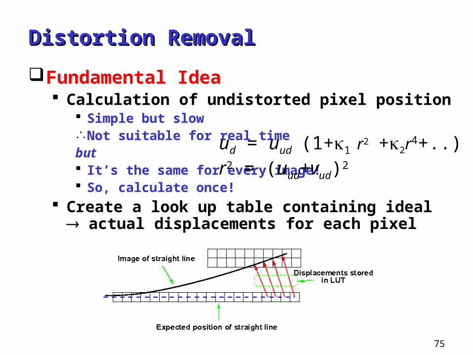
Distortion RemovalDistortion Removal

Fundamental Idea Calculation of undistorted pixel position

Simple but slowNot suitable for real timebut It’s the same for every image! So, calculate once!

Create a look up table containing ideal actual displacements for each pixel

ud = uud(1+1 r2 +2r

4+..)r2 = (uud+vud)2

76

Distortion RemovalDistortion Removal

Creating the LUT One entry (dx,dy) per pixel For a 1 Mpixel image needs 8 Mpixels!

Each entry is a float – (dx,dy) requires 8 bytes However, distortion is a smooth curve Store one entry per n pixels

Trials show that n=64 is OK for severely distorted image LUT row contains 210 / 2 6 = 24 = 16 entries Total LUT is 256 entries

Displacement for pixel j,k

dujk = (j mod 64) * uj/64,k/64

uj/64,k/64 is stored in LUT

Simple, fast circuit

Since the algorithm runs along scan lines,this multiplication is done by repeated addition

77

Alignment correctionAlignment correction

In general, cameras will not be perfectly aligned in canonical configuration

Also, may be using verging axes to improve depth resolution Calculate locations of epipolar lines once! Add displacements to LUT for distortion!

78

Real time 3D data acquisitionReal time 3D data acquisition

Real time stereo vision Implemented Gimel’farb’s Symmetric

Dynamic Programming Stereo in FPGA hardware

Real time precise stereo vision Faster, smaller hardware circuit Real time 3D maps

1% depth accuracy with 2 scan line latency at 25 frames/se

System block diagram: lens distortion removal,misalignment correction and depth calculator


79

Previous work: pros & consPrevious work: pros & consConventional approach: energy minimisation combining image

dissimilarity, surface curvature and occlusions• Exact minimisation with dynamic programming:

global 1D optimum matching under ordering constraints; can account for local photometric (offset or contrast) deviations and occlusions; fast processing;

no inter-scan-line constraints; random deviations on textureless regions; error propagation along scan-lines

• Approximate minimisation with Min-Cut techniques: 2D surface curvature constraints (MRF);

a provably close approximate solution of an NP-hard problem; can account for local occlusions;

cannot account for local or global photometric deviations; high computational complexity

• Heuristic approximate minimisation with Belief Propagation 2D surface curvature constraints (MRF);

can account for local occlusions; cannot account for local or global photometric deviations;

high computational complexity

80

Conventional approaches: Conventional approaches: basic problems basic problems

No account for intrinsic ill-posed nature of stereo problemsSearch for a single surface giving the best correspondence

between stereo imagesbut the single surface assumption is too restrictive in practice

Heuristic or empirical weights of energy terms dramatically affect matching accuracy

Large images and large disparity ranges lead to high computational cost of min-cut or belief propagation algorithms

81

Distribution of signal differences

Pixel-wise correspondences for a “Tsukuba” stereo pair (scan-line Pixel-wise correspondences for a “Tsukuba” stereo pair (scan-line y y = 173)= 173)

Grey-codedsignaldifferences

82

Concurrent Stereo Matching: Main ideasConcurrent Stereo Matching: Main ideas

Human ‘stroke-wise’ analysis of a 3D scene • Eyes browse from low to high frequency regions, from

sharp points to smooth areas rather than scan line-by-line (Torralba, 2003)

Appropriate (likely) correspondence rather than best matching

Separation of noise estimation and signal matching from selection of surfaces and occlusion handling

Stereo matching should avoid the ‘best match’ or signal difference minimisation almost universally

used nowin favour of a

likely match based on a local signal noise model

83

Modular structure of CSMModular structure of CSM

Step 1:Estimate the image noise model

(allow it to be spatially variant)

Segment based on noise

Select candidate 3D volumes

Step 2:Fit constrained surfaces to the

candidate volumes

Could use K-Mean, SUSAN, etc

Could be surface optimisation

84

Noise MapNoise Map

Scaled (Amplitudex6) Noise Map

White regions have higher noise - almost always

appears in occluded regions

Technique A: use a fast, efficient stereo matching technique (SDPS) to produce a disparity map – use mismatches as noise estimates

85

Noise-Driven SegmentationNoise-Driven Segmentation

Colour Mean Shift Segmentation

Colour-position clustering in a 5D feature space: 3D-colour model L*u*v and 2D-lattice coordinates

The noise map is considered to be the extra, sixth dimension

• Convert an image into data tokens• Choose initial search window

locations• Compute the ‘mean shift’ window

location for each initial position• Merge windows that end up on the

same ‘peak’ or mode• Cluster data over the merged

windows

After noise-driven segmentation: occluded regions are segmented into small isolated blocks

86

CSM: candidate 3D volumes and surface fittingCSM: candidate 3D volumes and surface fitting

Black regions contain likely matching points in the ‘slice’ for each disparity, d Surface fitting shrinks or expands each segmented region from slice to slice (based on counts of candidate points)

d= 5

d=8

d= 6

d=10d=9

d=12d=11 d=14d=13

d= 4

d= 7

d= 3

87

CSM: candidate 3D volumes and surface fittingCSM: candidate 3D volumes and surface fitting

Ideal disparity slices

CSM surface fitting

d=5 d=8d=6 d=10d=9

d=12d=11 d=14d=13 Disparity map

d=5 d=8d=6 d=10d=9

d=12d=11 d=14d=13 CSM Disparity map

88

Symmetric CSM: Symmetric CSM: candidate 3D volumes and surface fittingcandidate 3D volumes and surface fitting

d=5

d=8

d=6

d=10d=9

d=12d=11 d=14d=13

d=7

d=3 d=4

89

Symmetric CSM: Symmetric CSM: candidate 3D volumes and surface fittingcandidate 3D volumes and surface fitting

Ideal disparity slices

SCSM surface fitting

d=5 d=8d=6 d=10d=9

d=12d=11 d=14d=13 Disparity map

d=5 d=8d=6 d=10d=9

d=12d=11 d=14d=13 SCSM Disparity map

90

Algorithm ComparisonAlgorithm Comparison

Symmetric DP stereo Graph cut Symmetric BP

SCSM CSM Ground Truth

91

Middlebury Benchmark (MB)Middlebury Benchmark (MB)

Algorithms

Tsukuba Sawtooth

all untex disc all untex disc

MB-SBPO 0.97 1 0.28 3 5.45 3 0.19 1 0.00 1 2.09 3

CSM 1.15 3 0.80 12 1.86 2 0.98 13 0.62 25 1.69 2

SCSM 0.97 1 0.74 11 1.80 1 0.96 12 0.60 24 1.57 1

* MB-SBPO – symmetric belief propagation algorithm (best-performing Middlebury benchmark)

Algorithms

Venus Map

all untex disc all disc

MB-SBPO 0.16 3 0.02 3 2.77 1 0.16 1 2.20 1

CSM 1.18 12 1.04 10 1.48 3 3.08 34 7.34 18

SCSM 1.15 11 0.91 9 1.38 2 3.05 33 7.03 17

rank among 40

algorithms

92

ConclusionsConclusions

Stereo matching is an ill-posed problem, reconstruction of actual 3D optical surfaces is impracticalMore reasonable goal: mimic human binocular stereo vision

Conventional constrained best matching does not explicitly account for a multiplicity of equivalent matches, for noise in both images of a stereo pair and for local contrast or offset image distortions

Concurrent stereo matching gives promising results because it separates the problem into • search for all the candidate volumes with equivalent good matches

(allowing for the estimated noise) and • search for surfaces fitting to the volumes

Even the simplest implementation of the new approach competes with the best-performing conventional algorithms

Sloping surfaces challenge our CSM algorithm – watch this space!

93

IVCNZ’2006IVCNZ’2006

For a conference with a different style, consider IVCNZ’2006(Image and Vision Computing, New Zealand)

Great Barrier Island, New Zealand• Gateway to the Hauraki Gulf

and Auckland• 40 mins by light plane from

Auckland,3 hours by ferry

• Full range of accommodation options:

• Hotel style, cabins, … , even tents!

Book early and

you can sail there

94

Great Barrier IslandGreat Barrier Island

95

Stereo: Correspondence ProblemStereo: Correspondence Problem

Stereo Pair Images from identical cameras separated by some distance

to produce two distinct views of a scene

xL xR

Disparity = xL - xR 1z

Corresponding RegionsLeft Image Right Image

Documents

Image Noise John Morris Department of Computer Science, Tamaki Campus The University of Auckland