Image is NOT Perfect Sometimes EE465: Introduction to Digital Image Processing 1

Image is NOT Perfect Sometimes

EE465: Introduction to Digital Image Processing 1

Image Enhancement for Visually Impaired Patients


http://www.eri.harvard.edu/faculty/peli/projects/enhancement.html


Image Enhancement

Introduction Spatial domain techniques

Point operations Histogram equalization and matching Applications of histogram-based

enhancement Frequency domain techniques

Unsharp masking Homomorphic filtering*


Recall: There is no boundary of imagination in the

virtual world In addition to geometric transformation

(warping) techniques, we can also photometrically transform images Ad-hoc tools: point operations Systematic tools: histogram-based methods Applications: repair under-exposed or over-

exposed photos, increase the contrast of iris images to facilitate recognition, enhance microarray images to facilitate segmentation.


Point Operations Overview

Point operations are zero-memory operations wherea given gray level x[0,L] is mapped to anothergray level y[0,L] according to a transformation

)(xfy

L

L

x

y

L=255: for grayscale images


Lazy Man Operation

L

L

x

y

xy

No influence on visual quality at all


Digital Negative

xLy

L x0

L


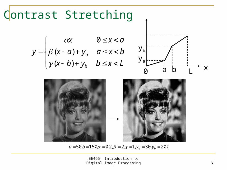
Contrast Stretching

Lxbybx

bxayax

axx

y

b

a

)(

)(

0

L x0 a b

ya

yb

200,30,1,2,2.0,150,50 ba yyba


Clipping

Lxbab

bxaax

ax

y

)(

)(

00

L x0 a b

2,150,50 ba


Range Compression

)1(log10 xcy

L x0

c=100


Summary of Point Operation

So far, we have discussed various forms of mapping function f(x) that leads to different enhancement results MATLAB function >imadjust

The natural question is: How to select an appropriate f(x) for an arbitrary image?

One systematic solution is based on the histogram information of an image Histogram equalization and specification


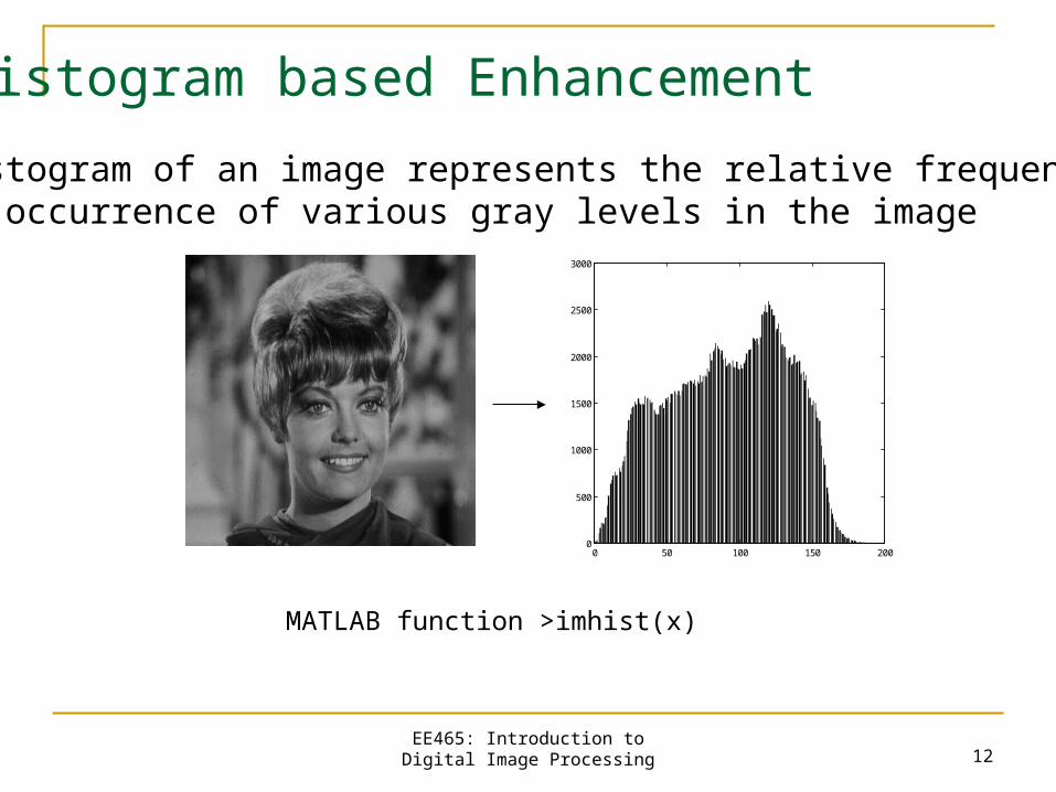
Histogram based Enhancement

Histogram of an image represents the relative frequency of occurrence of various gray levels in the image

0 50 100 150 2000

500

1000

1500

2000

2500

3000

MATLAB function >imhist(x)


Why Histogram?

Histogram information reveals that image is under-exposed

0 50 100 150 200 250

0

0.5

1

1.5

2

2.5

3

3.5

4

x 104

It is a baby in the cradle!


Another Example

0 50 100 150 200 250

0

1000

2000

3000

4000

5000

6000

7000

Over-exposed image


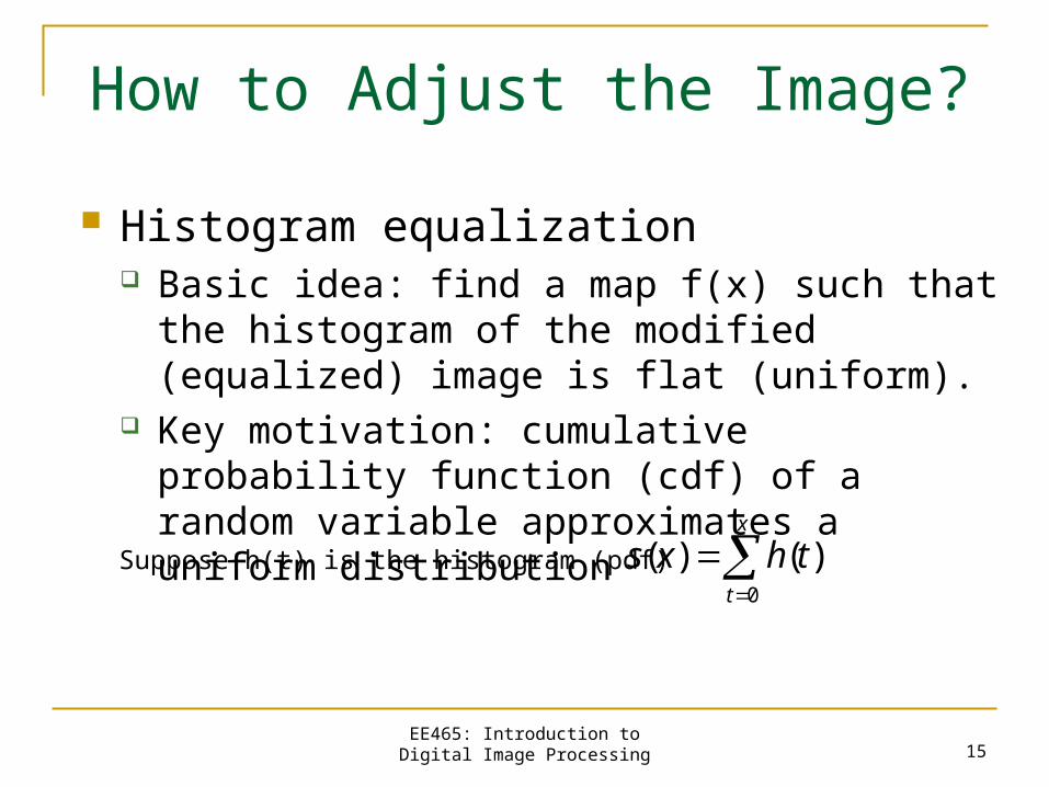
How to Adjust the Image?

Histogram equalization Basic idea: find a map f(x) such that the histogram

of the modified (equalized) image is flat (uniform). Key motivation: cumulative probability function

(cdf) of a random variable approximates a uniform distribution

x

t

thxs0

)()(Suppose h(t) is the histogram (pdf)

EE465: Introduction to Digital Image Processing

16

Histogram Equalization

x

t

thLy0

)(Uniform

Quantization

L

t

th0

1)(Note:

L

1

x

t

ths0

)(

x

L

y

0

cumulative probability function

http://en.wikipedia.org/wiki/Inverse_transform_sampling


MATLAB Implementation

function y=hist_eq(x)

[M,N]=size(x);for i=1:256 h(i)=sum(sum(x= =i-1));End

y=x;s=sum(h);for i=1:256 I=find(x= =i-1); y(I)=sum(h(1:i))/s*255;end

Calculate the histogramof the input image

Perform histogramequalization


Image Example

before after


Histogram Comparison

0 50 100 150 2000

500

1000

1500

2000

2500

3000

0 50 100 150 200 250 3000

500

1000

1500

2000

2500

3000

before equalization after equalization

Adaptive Histogram Equalization


http://en.wikipedia.org/wiki/Adaptive_histogram_equalization

EE565 Advanced Image Processing Copyright Xin Li 2008 21

Histogram Specification/Matching

ST

S-1*T

histogram1 histogram2

?

Given a target image B, how to modify a given image A such thatthe histogram of the modified A can match that of target image B?


Application (I): Digital Photography


Application (II): Iris Recognition

before after


Application (III): Microarray Techniques

before after


Application (IV)

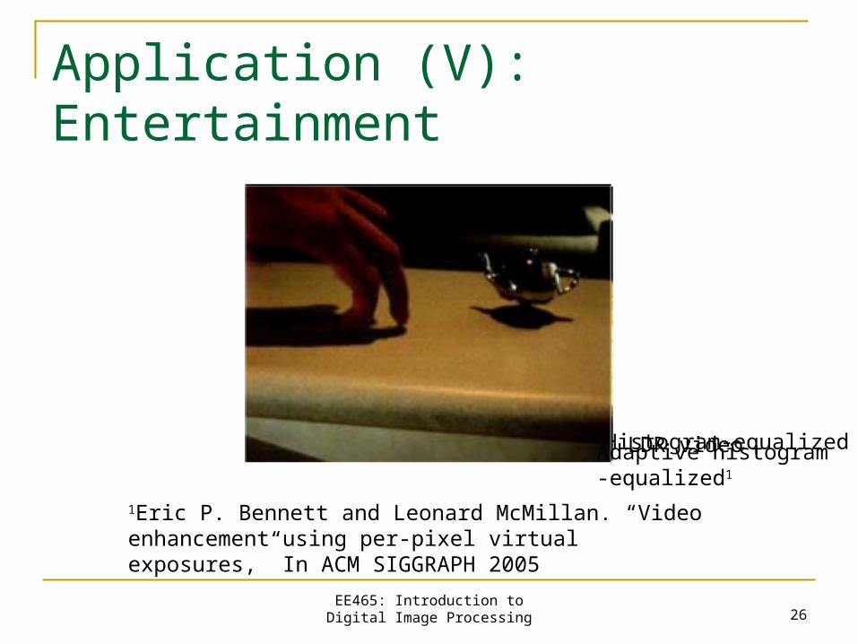
Application (V): Entertainment


LDR videoHistogram-equalizedAdaptive histogram-equalized1

1Eric P. Bennett and Leonard McMillan. “Video enhancement using per-pixel virtual exposures,” In ACM SIGGRAPH 2005


Image Enhancement

Introduction Spatial domain techniques

Point operations Histogram equalization and matching Applications of histogram-based

enhancement Frequency domain techniques

Unsharp masking Homomorphic filtering*


Frequency-Domain Techniques (I): Unsharp Masking

0),,(),(),( nmgnmxnmy

g(m,n) is a high-pass filtered version of x(m,n)

• Example (Laplacian operator)

)]1,()1,(

),1(),1([4

1),(),(

nmxnmx

nmxnmxnmxnmg


MATLAB Implementation

% Implementation of Unsharp masking

function y=unsharp_masking(x,lambda)

% Laplacian operationh=[0 -1 0;-1 4 -1;0 -1 0]/4;dx=filter2(h,x);y=x+lambda*dx;


0 50 100 150 200 2500

50

100

150

200

250

1D Example

0 50 100 150 200 2500

50

100

150

200

250

0 50 100 150 200 250 300-8

-6

-4

-2

0

2

4

6

8

0 50 100 150 200 250 30080

100

120

140

160

180

200

220

x(n) xlp(n)

g(n)=x(n)-xlp(n) )()()( ngnxny


2D Example

>roidemoMATLAB command


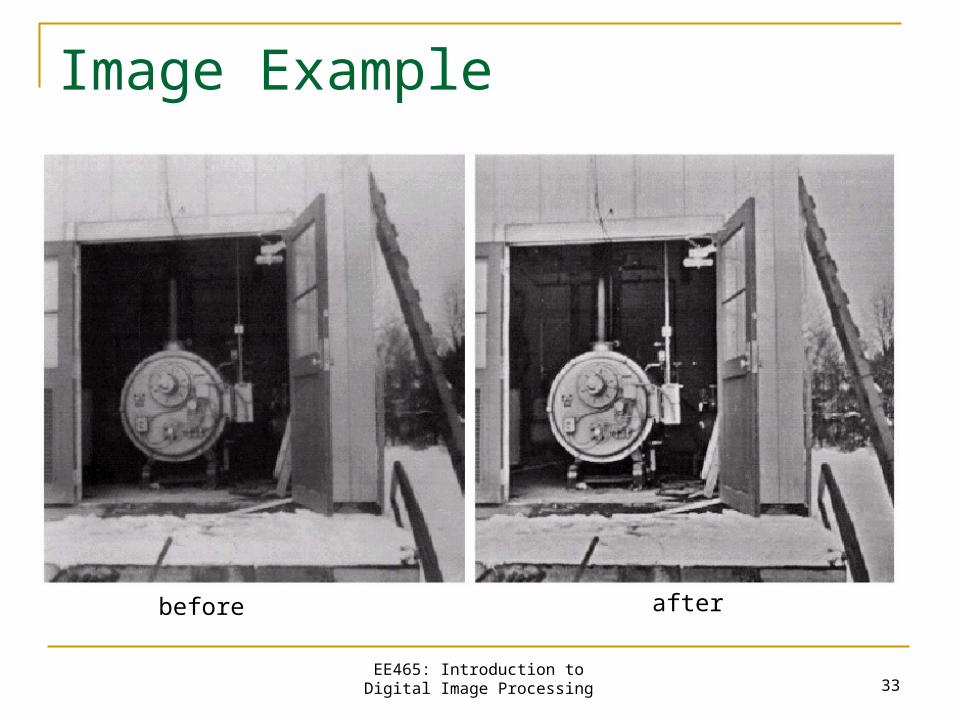
Frequency-Domain Techniques (II): Homomorphic filtering

),(),(),( yxryxiyxf

Illumination(low freq.)

reflectance(high freq.)

Basic idea:

),(ln),(ln),(ln yxryxiyxf

freq. domain enhancement


Image Example

before after


Summary of Nonlinear Image Enhancement Understand how image degradation occurs first

Play detective: look at histogram distribution, noise statistics, frequency-domain coefficients…

Model image degradation mathematically and try inverse-engineering

Visual quality is often the simplest way of evaluating the effectiveness, but it will be more desirable to measure the performance at a system level Iris recognition: ROC curve of overall system Microarray: ground-truth of microarray image segmentation

result provided by biologists

Documents

Image is NOT Perfect Sometimes EE465: Introduction to Digital Image Processing 1