Embed Size (px)
DESCRIPTION
Image Analysis for Automatic Phenotyping. Chris Glasbey , Graham Horgan , Yu Song Biomathematics and Statistics Scotland (BioSS) Gerie van der Heijden, Gerrit Polder Biometris, Wageningen UR. Wageningen , 7 March 2012. Manual phenotyping. - PowerPoint PPT Presentation
Citation preview

Image Analysis for Automatic PhenotypingImage Analysis for Automatic Phenotyping
Chris Glasbey, Graham Horgan, Yu SongChris Glasbey, Graham Horgan, Yu SongBiomathematics and Statistics Scotland (BioSS)Biomathematics and Statistics Scotland (BioSS)
Gerie Gerie van der Heijden, Gerrit Polder van der Heijden, Gerrit Polder Biometris, Biometris, Wageningen URWageningen UR
Wageningen, 7 March 2012Wageningen, 7 March 2012

Manual phenotyping
Disadvantages: - Slow and expensive- Variation between observers - Sometimes destructive

Phenotyping by Image Analysis
• Most image analysis systems for automatic phenotyping bring the plants to the camera.
Sorting Anthurium cuttings, Wageningen UR
Scanalyzer 3D, LemnaTec

Commercial tomato plants
in Almeria, Spain
But for some crops, like pepper and tomato, this is not feasible bring the cameras to the plants!
Pepper plants
in our experiments
SPYSEEequipment

4* IR, Colour, Range (ToF)cameras
SPYSEE
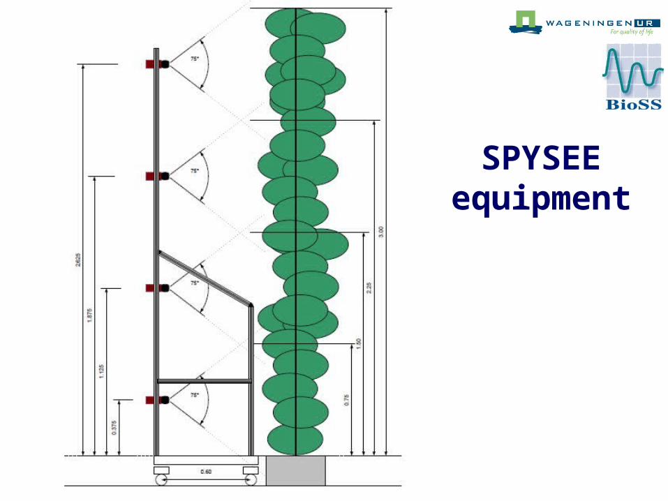
Plan
We aim to : • Replace manual by automatic measurements• Find new features, which are not possible or
too difficult for manual measurement
Two approaches:
1. 3D2. Statistical

1. 3D approach
3D information can be recoveredfrom stereo pairs, because
Depth = constant / disparity

Objects close to camera move faster than those far away.
Source: Parallax scrolling from Wikipedia

Stereo pair + ToF range image detailed range image

Foreground leavesForeground leaves

Leaf in 3D automatic measurement of size, orientation, etc

Validation trial (11 genotypes, 55 leaves): Correlation = 98% RMSE = 9.50cm2
Automatic
Manual
Individual leaf size (cm2)

• Leaf size had a heritability of 0.70, three QTLs were found, together explaining 29% of the variation.
QTL analysis of automatically measured leaf sizes for 151 genotypes
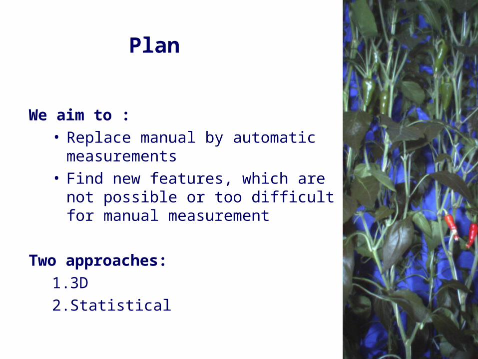
Leaf orientation:
• Angle between the leaf and the vertical axis.

Leaf orientation:
• Angle between the leaf and the vertical axis.
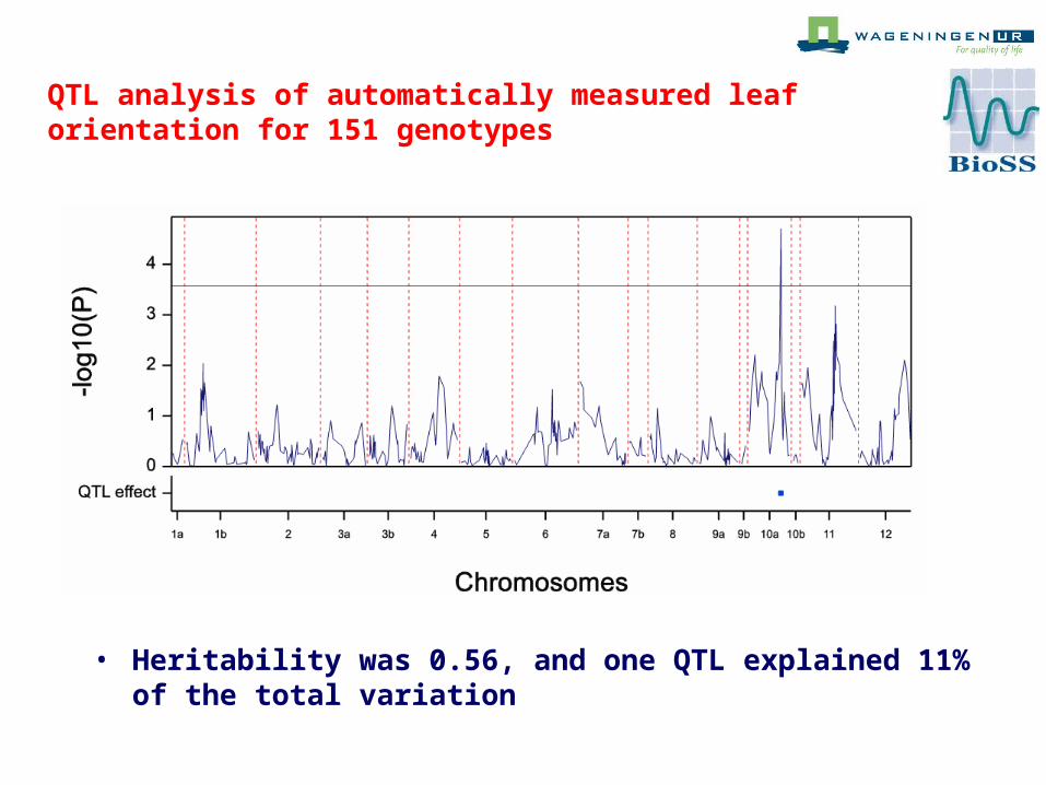
• Heritability was 0.56, and one QTL explained 11% of the total variation
QTL analysis of automatically measured leaf orientation for 151 genotypes

Plant height estimated, from locations of ‘green’ pixels
2. Statistical approach

Correlation 93% between automatic and manual plant
heights

Total leaf area is a measure of how much solar radiation the plant can intercept
0 50 100 150 200 250
05
00
10
00
15
00
20
00
25
00
Intensity
Fre
qu
enc
y
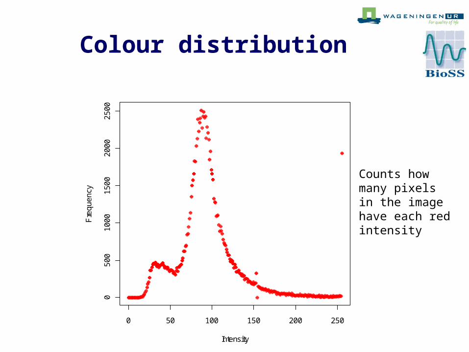
Colour distribution
Counts how many pixels in the image have each red intensity

Colour distribution
0 50 100 150 200 250
05
00
10
00
15
00
20
00
25
00
Intensity
Fre
qu
en
cy

0 50 100 150 200 250
05
00
10
00
15
00
20
00
25
00
30
00
Intensity
Fre
qu
en
cy
Another example
Colour histograms
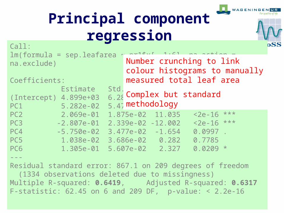
Call:lm(formula = sep.leafarea ~ pr1$x[, 1:6], na.action = na.exclude)
Coefficients: Estimate Std. Error t value Pr(>|t|) (Intercept) 4.899e+03 6.288e+01 77.905 <2e-16 ***PC1 5.282e-02 5.473e-03 9.651 <2e-16 ***PC2 2.069e-01 1.875e-02 11.035 <2e-16 ***PC3 -2.807e-01 2.339e-02 -12.002 <2e-16 ***PC4 -5.750e-02 3.477e-02 -1.654 0.0997 . PC5 1.038e-02 3.686e-02 0.282 0.7785 PC6 1.305e-01 5.607e-02 2.327 0.0209 * ---Residual standard error: 867.1 on 209 degrees of freedom (1334 observations deleted due to missingness)Multiple R-squared: 0.6419, Adjusted R-squared: 0.6317 F-statistic: 62.45 on 6 and 209 DF, p-value: < 2.2e-16
Number crunching to link colour histograms to manually measured total leaf area
Complex but standard methodology
Principal component regression

Prediction vs manual
2000 4000 6000 8000
30
00
40
00
50
00
60
00
70
00
Total leaf area
Pre
dic
ted
pro
ject
e le
af a
rea
Correlation 80%

Regression coefficients
0 50 100 150 200 250
-0.0
6-0
.04
-0.0
20
.00
0.0
20
.04
Intensity
Co
effi
cie
nt
Weight of each colour intensity count in predicting the leaf area index

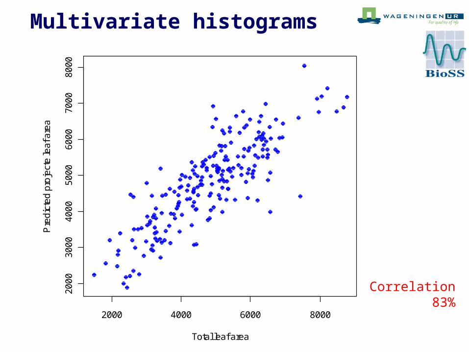
Multivariate histograms
• Count the number of times each combination of the three colour components occurs
• Too many possibilities, so use bins of length 8 per component, leading to 163 = 4096 variables
• Again do Principal Components regression
Multivariate histograms
2000 4000 6000 8000
20
00
30
00
40
00
50
00
60
00
70
00
80
00
Total leaf area
Pre
dic
ted
pro
ject
e le
af a
rea
Correlation 83%

• The heritability of total leaf area was 0.55, and 20% of the variation was explained by QTLs
• 2 QTLs agree with 2 of 3 found from manual measurements
QTL analysis of automatically measured total leaf area for 151 genotypes

Image Fruit Probability
Work in progress:
• Automatically find fruits
• Measure plant development

31 Aug 2 Sep 5 Sep 8 Sep 9 Sep

Summary
• The SPYSEE imaging setup records tall pepper plants while they are growing in a greenhouse
• Two approaches of automatic phenotyping have been explored:
1. 3D2. Statistical
• QTLs have be found using our approaches, and good agreement with some manual measurements were achieved