DART: A FAST HEURISTIC ALGEBRAIC RECONSTRUCTION ALGORITHMFOR DISCRETE TOMOGRAPHY

K.J. Batenburg and J. Sijbers

University of Antwerp, Vision LabUniversiteitsplein 1, B-2610, Wilrijk, Belgium

ABSTRACT

Discrete tomography (DT) is concerned with the tomo-graphic reconstruction of images that consist of only a smallnumber of gray levels. DT reconstruction problems are usu-ally underdetermined. Therefore, incorporation of heuristicrules to guide the reconstruction algorithm towards an opti-mal as well as intuitive solution would be valuable.

In this paper, we introduce DART: a new, heuristic DT al-gorithm that is based on an iterative algebraic reconstructionmethod. Starting from a continuous reconstruction, a discreteimage is reconstructed by consistent updating of border pix-els. Using simulation experiments, it is shown that the DARTalgorithm is capable of computing high quality reconstruc-tions from substantially fewer projections than required forconventional continuous tomography.

Index Terms— Discrete tomography, algebraic reconstruc-tion technique, image reconstruction

1. INTRODUCTION

Discrete tomography (DT) is concerned with the problem ofrecovering images from their projections where the imagesare assumed to consist of a small number of gray values only[1]. Potential benefits of DT are an increase of the recon-struction quality and a reduction of the required number ofprojection images. The DT reconstruction problem, however,is generally underdetermined and the number of possible so-lutions can be substantial. Therefore, incorporation of ad-ditional rules to guide the reconstruction process towardsanoptimal as well as intuitive solution would be valuable.

Several reconstruction algorithms for DT have been pro-posed, most of which are limited to the reconstruction of bi-nary images (i.e., black-and-white) [2–4].

In this paper, we propose a new, heuristic DT algorithmthat is based on an iterative algebraic reconstruction algo-rithm. The method will be referred to as DART (DiscreteAlgebraic Reconstruction Technique). After introducing ba-sic notations and concepts in Section 2.1, an overview of the

This work was financially supported by the the F.W.O. (Fund for Scien-tific Research - Flanders, Belgium)

DART algorithm is given in Section 2.2, which will be elab-orated on in Section 2.3. Finally, in Section 3, simulationresults are presented and discussed.

2. METHOD

2.1. Notation and concepts

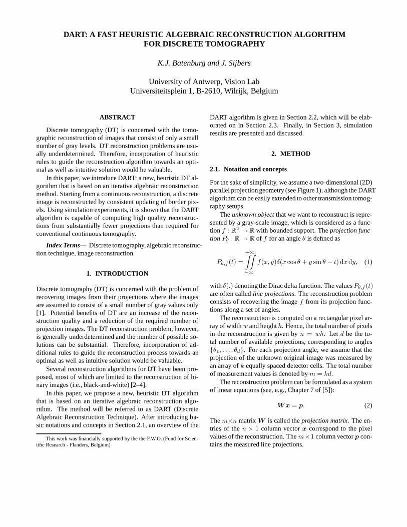
For the sake of simplicity, we assume a two-dimensional (2D)parallel projection geometry (see Figure 1), although the DARTalgorithm can be easily extended to other transmission tomog-raphy setups.

Theunknown objectthat we want to reconstruct is repre-sented by a gray-scale image, which is considered as a func-tion f : R

2 → R with bounded support. Theprojection func-tion Pθ : R → R of f for an angleθ is defined as

Pθ,f(t) =

+∞∫∫

−∞

f(x, y)δ(x cos θ + y sin θ − t) dxdy, (1)

with δ(.) denoting the Dirac delta function. The valuesPθ,f(t)are often calledline projections. The reconstruction problemconsists of recovering the imagef from its projection func-tions along a set of angles.

The reconstruction is computed on a rectangular pixel ar-ray of widthw and heighth. Hence, the total number of pixelsin the reconstruction is given byn = wh. Let d be the to-tal number of available projections, corresponding to angles{θ1, . . . , θd}. For each projection angle, we assume that theprojection of the unknown original image was measured byan array ofk equally spaced detector cells. The total numberof measurement values is denoted bym = kd.

The reconstruction problem can be formulated as a systemof linear equations (see, e.g., Chapter 7 of [5]):

Wx = p. (2)

Them×n matrix W is called theprojection matrix. The en-tries of then × 1 column vectorx correspond to the pixelvalues of the reconstruction. Them×1 column vectorp con-tains the measured line projections.

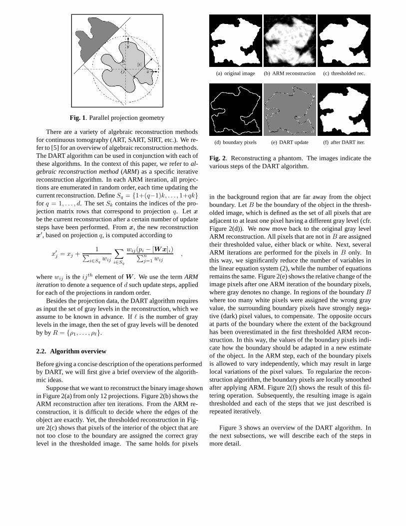
Fig. 1. Parallel projection geometry

There are a variety of algebraic reconstruction methodsfor continuous tomography (ART, SART, SIRT, etc.). We re-fer to [5] for an overview of algebraic reconstruction methods.The DART algorithm can be used in conjunction with each ofthese algorithms. In the context of this paper, we refer toal-gebraic reconstruction method(ARM) as a specific iterativereconstruction algorithm. In each ARM iteration, all projec-tions are enumerated in random order, each time updating thecurrent reconstruction. DefineSq = {1+(q−1)k, . . . , 1+qk}for q = 1, . . . , d. The setSk contains the indices of the pro-jection matrix rows that correspond to projectionq. Let x

be the current reconstruction after a certain number of updatesteps have been performed. Fromx, the new reconstructionx′, based on projectionq, is computed according to

x′

j = xj +1

∑

i∈Sqwij

∑

i∈Sq

wij(pi − [Wx]i)∑n

j=1wij

,

wherewij is theijth element ofW . We use the termARMiteration to denote a sequence ofd such update steps, appliedfor each of the projections in random order.

Besides the projection data, the DART algorithm requiresas input the set of gray levels in the reconstruction, which weassume to be known in advance. Ifℓ is the number of graylevels in the image, then the set of gray levels will be denotedby byR = {ρ1, . . . , ρℓ}.

2.2. Algorithm overview

Before giving a concise description of the operations performedby DART, we will first give a brief overview of the algorith-mic ideas.

Suppose that we want to reconstruct the binary image shownin Figure 2(a) from only 12 projections. Figure 2(b) shows theARM reconstruction after ten iterations. From the ARM re-construction, it is difficult to decide where the edges of theobject are exactly. Yet, the thresholded reconstruction inFig-ure 2(c) shows that pixels of the interior of the object that arenot too close to the boundary are assigned the correct graylevel in the thresholded image. The same holds for pixels

(a) original image (b) ARM reconstruction (c) thresholded rec.

(d) boundary pixels (e) DART update (f) after DART iter.

Fig. 2. Reconstructing a phantom. The images indicate thevarious steps of the DART algorithm.

in the background region that are far away from the objectboundary. LetB be the boundary of the object in the thresh-olded image, which is defined as the set of all pixels that areadjacent to at least one pixel having a different gray level (cfr.Figure 2(d)). We now move back to the original gray levelARM reconstruction. All pixels that are not inB are assignedtheir thresholded value, either black or white. Next, severalARM iterations are performed for the pixels inB only. Inthis way, we significantly reduce the number of variables inthe linear equation system (2), while the number of equationsremains the same. Figure 2(e) shows the relative change of theimage pixels after one ARM iteration of the boundary pixels,where gray denotes no change. In regions of the boundaryB

where too many white pixels were assigned the wrong grayvalue, the surrounding boundary pixels have strongly nega-tive (dark) pixel values, to compensate. The opposite occursat parts of the boundary where the extent of the backgroundhas been overestimated in the first thresholded ARM recon-struction. In this way, the values of the boundary pixels indi-cate how the boundary should be adapted in a new estimateof the object. In the ARM step, each of the boundary pixelsis allowed to vary independently, which may result in largelocal variations of the pixel values. To regularize the recon-struction algorithm, the boundary pixels are locally smoothedafter applying ARM. Figure 2(f) shows the result of this fil-tering operation. Subsequently, the resulting image is againthresholded and each of the steps that we just described isrepeated iteratively.

Figure 3 shows an overview of the DART algorithm. Inthe next subsections, we will describe each of the steps inmore detail.

Compute a start reconstructionx0 using ARM;

t := 0;

while (stop criterion is not met)dobegin

t := t + 1;

Compute the segmented imagest = r(xt−1);

Compute the setIt of non-boundary pixels ofst;

Compute the imageyt from xt−1 andst, settingyt

i := st

i if i ∈ It andyt

i := xt−1

iotherwise;

Usingyt as the start solution, compute the ARM reconstructionxt, while keeping the pixels inI fixed;

Apply a smoothing operation to the pixels that are not inI ;

end

Fig. 3. Basic steps of the DART algorithm.

2.3. Algorithm description

The first approximate reconstructionx0 is computed usingthe continuous ARM algorithm. For all DT experiments inSection 3 we used three ARM iterations.

Each time a (partially) continuous reconstruction has beencomputed, it is segmented to obtain an imagest that has onlygray levels from the setR = {ρ1, . . . , ρℓ}. For all exper-iments in this paper we used global thresholding with fixedthresholds to perform this segmentation. Fori = 1, . . . , ℓ−1,define

τi =ρi + ρi+1

2.

Define thethreshold functionr : R → R as

r(v) =

ρ1 (v < τ1)ρ2 (τ1 ≤ v < τ2). . .

ρℓ (τℓ−1 ≤ v).

. (3)

As a shorthand notation we also define the threshold func-tion of animagex ∈ R

n: r(x) =(

r(x1) . . . r(xn))T

.

After the segmented reconstructionst = r(xt−1) hasbeen computed, the setIt of non-boundary pixelsis com-puted from the segmented image. A pixelst

i is called a non-boundary pixel if all pixels from its 8-connected neighbor-hood have the same gray level inst. The remaining set ofpixels,Bt, are called theboundary pixels.

Then, the imageyt is computed fromxt−1 andst, settingyt

i := sti if i ∈ It andyt

i := xt−1

i if i ∈ Bt.

Consider the system of linear equations

| |w1 · · · wn

| |

x1

· · ·xn

= p, (4)

wherewi denotes theith column vector ofW . We now de-fine the operation offixing a variablexi at valuevi ∈ R. Ittransforms the system (4) into the new system

| | | |w1 · · · wi−1 wi+1 · · · wn

| | | |

x1

· · ·xi−1

xi+1

· · ·xn

= p−viwi.

(5)The new system has the same number of equations as the orig-inal system, whereas the number of variables is decreased byone.

Using the imageyt as the start solution, the new recon-structionxt is computed by applying a single ARM iteration,keeping all non-boundary pixels fixed.

Finally, a local smoothening operator is applied to the pix-els in the setBt, settingxt

i := 0.7xti + 0.3b, whereb denotes

the average gray value in the 8-neighborhood of pixeli.To determine when the algorithm should terminate, we

use thetotal projection errorE : Rn → R, defined as

E(x) = |Wx − p|2.

The algorithm is terminated after the total projection error ofthe best reconstruction found so far has not decreased duringthe last10 iterations. The termination check is computation-ally expensive by itself, and is therefore only performed aftereach multiple of 10 main loop iterations. We also used a fixedupper bound of 500 main loop iterations, which was neverreached in the experiments for this paper.

3. EXPERIMENTAL RESULTS

We implemented the DART algorithm in C++, using the gcccompiler. All experiments were performed on an Intel E6700PC, using a single CPU core.

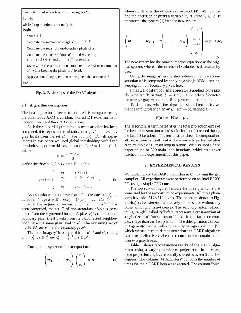
The top row of Figure 4 shows the three phantoms thatwere used for the reconstruction experiments. All three phan-toms have size512×512 pixels. The phantom shown in Fig-ure 4(a), calledsimpleis a relatively simple shape without anyholes, although it is not convex. The second phantom, shownin Figure 4(b), calledcylinders, represents a cross-section ofa cylinder head from a motor block. It is a far more com-plex shape than the first phantom. The third phantom, shownin Figure 4(c) is the well-known Shepp-Logan phantom [5],which we use here to demonstrate that the DART algorithmcan be used effectively when the reconstruction contains morethan two gray levels.

Table 1 shows reconstruction results of the DART algo-rithm, using a varying number of projections. In all cases,thed projection angles are equally spaced between0 and180degrees. The column “#DART iters” contains the number oftimes the main DART loop was executed. The column “pixel

error” indicates the fraction of pixels for which the recon-struction is different from the phantom image. The last col-umn shows the total running time.

Note that we use a different number of projections foreach phantom. The results for the two binary phantoms showthat there is a sharp lower bound on the number of projectionsthat are required for a reconstruction of high quality. For ex-ample, for thecylindersphantom, using 9 projections resultsin a pixel error of 0.83, whereas using 10 or more projectionssuddenly makes the pixel error drop below 0.002. For eachof the phantoms we experimentally determined the minimalnumber of required projections, indicated by a bold font inTable 1.

The second row of Figure 4 shows ARM reconstruction ofthe three phantoms, after ten iterations. The number of pro-jections used in Figure 4(d), 4(e), and 4(f) are 5, 10, and 18,respectively. Finally, the last row of Figure 4 shows DARTreconstructions of the phantom images. The DART recon-structions are based on the same number of projections as theARM reconstructions in the middle row.

(a) Simple (b) Cylinders (c) Shepp-Logan

(d) ARM: 5 proj. (e) ARM: 10 proj. (f) ARM: 18 proj.

(g) DART: 5 proj. (h) DART: 10 proj. (i) DART: 18 proj.

Fig. 4. (a-c): original phantom images; (d-f): ARM recon-structions; (g-i): DART reconstructions.

The results show that for each of the phantoms, the DARTalgorithm is capable of computing an accurate reconstructionfrom a significantly smaller number of projections than re-quired by the ARM algorithm to obtain similar quality. To thebest of our knowledge, there are currently no DT reconstruc-tion results for images larger than256×256 in the literature.

phantom d #DART pixel error running timeiters (sec.)

4 120 0.03557 8.7Simple 5 110 0.00042 9.4

6 90 0.00026 8.69 130 0.08303 18.7

Cylinders 10 110 0.00175 17.411 120 0.00167 20.512 110 0.14213 22.5

Shepp- 15 60 0.08440 15.3Logan 18 100 0.02567 29.6

21 80 0.02355 27.4

Table 1. Experimental results for the three phantoms, usingperfect projection data

Even for the phantom images of size512×512, the DART al-gorithm required less than half a minute computation time inall cases. An interesting question, which we consider to beout of the scope of this paper, is how the minimal number ofrequired projections can be determined a priori.

4. CONCLUSIONS

We have presented a new iterative algebraic reconstructionalgorithm for discrete tomography, called DART. The DARTalgorithm combines the efficiency of iterative algebraic meth-ods from continuous tomography with the power of discretetomography to compute accurate reconstructions from rela-tively few projections.

Our experimental results demonstrate that the DART al-gorithm is capable of computing reconstructions of very highquality from a small number of projections. The algorithmis very effective for binary images, but it can also be used toreconstruct images that contain more than two gray levels.

5. REFERENCES

[1] G.T. Herman and A. Kuba, Eds.,Discrete Tomography:Foundations, Algorithms and Applications, Birkhauser,Boston, 1999.

[2] K.J. Batenburg, “A network flow algorithm for binary im-age reconstruction from few projections,”Lecture NotesComp. Sci., vol. 4245, pp. 86–97, 2006.

[3] S. Weber, A. Nagy, Th. Schule, C. Schnorr, and A. Kuba,“A benchmark evaluation of large-scale optimization ap-proaches to binary tomography,”Lecture Notes Comp.Sci., vol. 4245, pp. 146–156, 2006.

[4] G.T. Herman and A. Kuba, Eds.,Advances in DiscreteTomography and its Applications, Birkhauser, Boston,2007.

[5] A.C. Kak and M. Slaney, Principles of ComputerizedTomographic Imaging, SIAM, 2001.