Embed Size (px)
Citation preview

D-A125"619 EVALUATION OF THE PERFORMANCE AND FLOW IN AN AXIALCOMPRESSOR(U) NAVAL POSTGRADUATE SCHOOL MONTEREY CA
NCL SSIFIED J L WADDELL OCT 82 F/G 13/7 NL
""IIIII"""IIIIIIIIIIIIIIII
11111mom
11111125 l jji 14 HI 16=
MICROCOPY RESOLUTION TEST CHART
NATIONAL BUREAU OF STANDARDS 1963 A
momIe A

NAVAL POSTGRADUATE SCHOOLMonterey, California
THESISEVALUATION OF T"HE PERFORMANCE AND
FLOW IN AN AXIAL COMPRESSOR
by
Joh-n Leighton Waddell]
October 1982
Thesis Advisor: R. P. Shreeve
rRApproved for public release; distr 4bu-ion unlimited
803 14 045 -4

UNCLASS IFIlEDSECURITY CLASSIFICATION OF T14S PA f9* Dole zaaei_________________
REPOT OOCUMENTATION PAGE ____________________
1. REPORT RUNERM Ict,, GOTACIINN EIPET A LGNd
4. TITLE twd Staboeft) TYPE OF REPORT 6 PERmOo COVERhED
Master's ThesisEvaluation of the Performance and October 1982Flow in an Axial Compressor *.PERFORNING ONG. REPORT N-iffeRa
7. AUTHOR.* G. CONTRACT 0ORAM M1RAN T ERf78j
John Leighton Waddell
S. PERFORMING 0111GANIZATION N~A AND ADDRESS PR8~ LMT. PROjeCT, TASK
N'aval Postgraduate SchoolMonterey, California 93940
St. CONTROLLING OFFICE NAME AND AGGRESS 12. REPORT *ATR
Naval Postgraduate School October 1982Monterey, California 93940 13. NUNGIRR Of PAGES
14. MONITORING AGENCY NAME &A001181f ADRESnft se e Cave"Wlj Ofie 16SCUIT CLASS. (of this "i.,wjt
Unclassified
09 OCLASSIVICATIONW ONGRAOING
14. OISTI1aUTION STATEMENT (of110119 Rep.W)
Approved for public release; distribution unlimited
17. OISTRISUTION STATEMENT (of fhe 46611 44 019~ 101 Alsoit Of i dtfla.*f h~- Reft%)
Is. SUPPLEMENTARY NOTES
to. Key WORDS (Caofiuue '9n g fe e @04 A*600wit ad*8eo orN 1140*ad owe)
Secondary Flows
Guide VanesCompressor Testing
20. AGSYMACT (Cea~ 0 PWg 61411 uit 011404MVeAp d 141111016 6F o Mesh O. )
An experimental evaluation of the axial compressor testrig with one stage of symmetric blading was conducted to de-termine its suitability for studies of tip clearance effects.*1 Measurements were made of performance parameters and internalflow fields. The configuration tested was found to be un-suitable due to poor flow from th,-e inlet guide vanes, par-ticularly near the tip region. Secondary flows and flaws in
DO F'~t"F 1473 corTioN or I Nov Gois OnsoLeTt UNCLASSIFIEDSECURITY CLASSFICATION OF THIS PAGE (1101411 0016 Siwepd)
MEO

UNCLASSIFIED
construction of the guide vanes were suggested as probablecauses. Recommendations were made for a program to resolvethe problem.
Accession For
NTIS G!RA&IDTIC TAB EUnannounced EJust if i cation
By --
Distribution/ -fI O
Availability CodesjAvail and/or We
Dist Special
DDFrm 1473 2 UNCLASSIFIEDSP4 Oi'2-n14-6601 1C0"CIMIAINO o$PG~t.De##00
Approved for public release; distribution unlimited
Evaluation of the Performance andFlow in an Axial Compressor
by
John Leighton WaddellLieutenant, United States Navy
B.S.A.E., Texas A&M University, 1974
Submitted in partial fulfillment of therequirements for the degree of
MASTER OF SCIENCE IN AERONAUTICAL ENGINEERING
from the
NAVAL POSTGRADUATE SCHOOLOctober 1982
Author:
Approved by: _ _ _ _ _ _ _ _ _ _ _ _ _ _ _ _ _ _ _ _ _
Thesis Advisor
Chairman, Department of Aeronautics
Dean of Science and Engineering
-
I
.3
- -. 9 --. dill

ABSTRACT
An experimental evaluation of the axial compressor test
rig with one stage of symmetric blading was conducted to de-
termine its suitability for studies of tip clearance effects.
Measurements were made of performance parameters and internal
flow fields. The configuration tested was found to be un-
suitable due to poor flow from the inlet guide vanes, par-
ticularly near the tip region. Secondary flows and flaws in
construction of the guide vanes were suggested as probable
causes. Recommendations were made for a program to resolve
the problem.
4
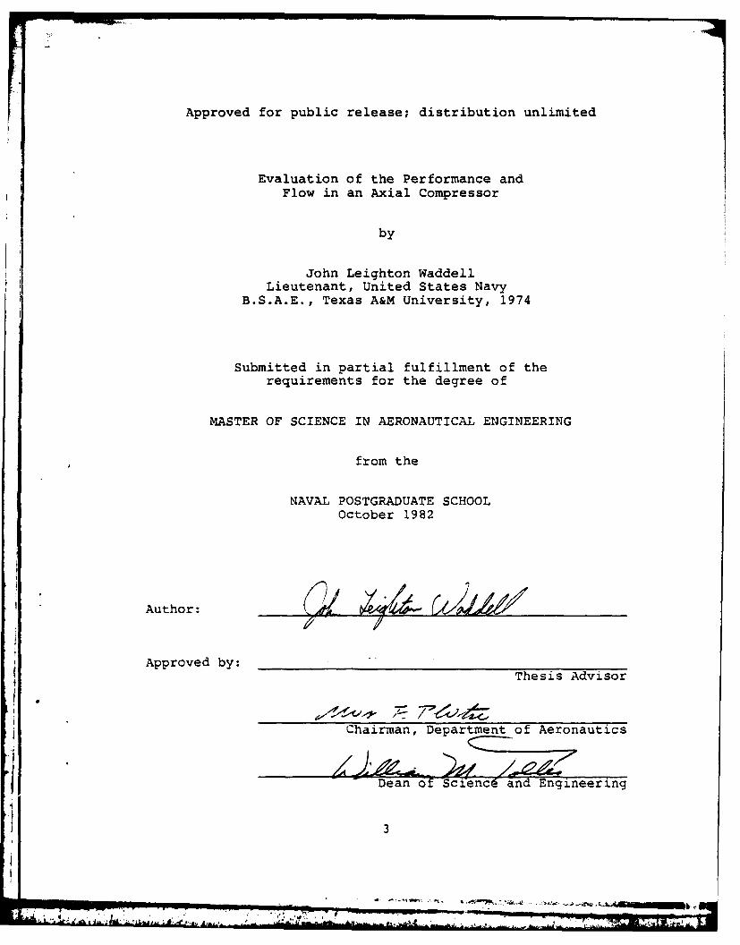
TABLE OF CONTENTS
I. INTRODUCTION................. .. ................ 15
II. APPARATUS..........................17
A. COMPRESSOR TEST RIG....................17
B. DATA ACQUISITION SYSTEM...............19
C. INSTRUMENTATION.....................19
III. TEST PROGRAM AND RESULTS.................24
A. SUMMARY...........................24
B. PHASE 1.........................24
C. PHASE 2.......................26
D. PHASE 3.........................29
E. SUPPLEMENTAL TESTS....................30
IV. DISCUSSION..........................33
A. FLOW FROM THE INLET GUIDE VANES.........33
B. PERFORMANCE DIFFERENCES.................37
C. MEASUREMENT UNSTEADINESS.................39
V. CONCLUSIONS AND RECOMMENDATIONS...........41
TABLES.................................43
FIGURES...................................79
APPENDIX A. SURVEY PROBE CALIBRATION.............132
APPENDIX B. COMPRESSOR DESIGN DATA..............141
APPENDIX C. EXPERIMENTAL DATA FROM BUILD 1........143
APPENDIX D. INTEGRATION OF EXIT RAKES...............145
fAPPENDIX E DATA REDUCTION EQUATIONS...........149
5

APPENDIX F. DATA REDUCTION SOFTWARE . . . . . .. .. .. 150
APPENDIX G. SUMMARY OF TEST PROGRAM . . . .. .. .. .. 155
LIST OF REFERENCES.......................138
INITIAL DISTRIBUTION LIST..................160
1 6

LIST OF TABLES
1. Measured Quantities, Typical Set-up . ....... . 43
2. Measurement Uncertainty .... ............. . 44
3. Performance Parameters (IGVs 00 ) .. ......... 45
4. Mid--span Velocity Vectors (IGVs 00 ) .. .. ....... 47
5. Mid-span Pressure Variations with Throttling (IGVs00) ....................... 49
6. Velocity Vectors at 17 Inches Radius (IGVs 00) 51
7. Pressure Variations at 17 Inches Radius (IGVs 0) 52
8. Performance Parameters (IGVs 40) .......... 53
9. Mid-span Velocity Vectors (IGVs 40) ....... .. 54
10. Mid-span Pressure Variations with Throttling (IGVs40) .... ....................... 55
11. Survey Results, Velocity Vectors (IGVs 00, S2+4) 56
12. Performance Parameters (IGVs 30) .......... 57
13. Mid-span Velocity Vectors (IGVs 30) .. .. ....... 58
14. Mid-span Pressure Variations with Throttling (IGVs30) . . . . . . . . . . . . . . . . . . . . . . 59
15. Survey Results, Velocity Vectors (IGVs 30, S2+4) 60
16. Survey Results, Velocity Vectors (IGVs 30, S1+4) 61
17. Survey Results, Velocity Vectors (IGVs 30, S1+2+4) 62
18. Performance Parameters (IGVs 20) ... .. ......... 63
19. Mid-span Velocity Vectors (IGVs 20) .. .. ....... 64
20. Mid-span Pressure Variations with Throttling (IGVs20) ..... ...... . . . .................... 65
21. Survey Results, Velocity Vectors (IGVs 20, S2+4) 66
7

22. Survey Results, Velocity Vectors (IGVs 20, S1+4) 67
23. Performance Parameters (IGVs 00 ) ..... ......... 68
24. Mid-span Velocity Vectors (IGVs 00) . ....... 69
25. Survey Results, Velocity Vectors (IGVs 0*, S1+4) . 70
26. Survey Results, Velocity Vectors (IGVs 00, S4) . 72
27. Survey Results, Velocity Vectors (IGVs 00, S2+3) . 74
28. Off Design Survey Velocity Vectors (IGVs 0, Sl) . 76
29. Off Design Survey Velocity Vectors (IGVs 00,S2+3+4) ....... ..................... 77
30. Velocity Vectors at Station One at Three Survey
Locations ....... .................... 78
Ala. "SMITH" Probe Coefficients .... ............ 135
Alb. "SMITH" Probe Calibration Errors .. ......... . 136
A2a. 539 Probe Coefficients ..... .............. 137
A2b. 539 Probe Calibration Errors ... ........... . 138
A3a. 538 Probe Coefficients ..... .............. 139
A3b. 538 Probe Calibration Errors ... ........... .. 140
BI. Summary of Mid-span Design Flow Values ....... .. 141
B2. Summary of Off Design Calculations .. ...... ... 142
Cl. Build 1 Velocities at Mid-Span ... .......... . 143
D1. Sub-Area Pressure Determination from ProbePressures ........ .................... 146
GI. Performance Map, Throttle Configurations ...... .. 157
8
.,. .

LIST OF FIGURES
1. Compressor Schematic ..... ............... 79
2. Measurement Planes for Installed Stage. ....... 80
3. Locations of Survey Ports .... ............. . 81
4. Performance Parameters vs Flow Rate (IGVs 00) . . 83
5. Comparison of Measured Performance with DesignValues and Build One Measurements ...... .... 84
6. Mid-span Flow Angles vs Flow Rate (IGVs 0) . .. 85
7. Flow Angles at 17 Inches Radius vs Flow Rate (IGVs0) ............................. 86
8. Inlet and Exit Pressure Distributions vs Radius at
Three Throttle Settings (IGVs 00 ) .......... 87
9. Performance Parameters vs Flow Rate (IGVs 40) 88
10. Mid-span Flow Angles vs Flow Rate (IGVs 40) .... 89
11. Inlet and Exit Pressure Distributions vs Radius atThree Throttle Settings (IGVs 40) .......... 90
12. Measured Flow Angle Radial Distribution at ModerateThrottling (IGVs 40, S2+S4; Design) . . . . 91
13. Relative Flow Angle Radial Distribution at ModerateThrottling (IGVs 40, S2+S4; Design) . . . . 92
14. Axial Velocity Radial Distribution at ModerateThrottling (IGVs 40, S2+S4) ... ............ . 93
15. Intrastage Pressure Radial Distributions at
Moderate Throttling (IGVs 40, S2+S4) . ....... 94
16. Performance Parameters vs Flow Rate (IGVs 30) . . 95
17. Mid-span Flow Angles vs Flow Rate (IGVs 30) . ... 96
18. Inlet and Exit Pressure Distributions vs Radius atThree Throttle Settings (IGVs 30) ... ......... 97
9
IL. t n - i

19. Measured Flow Angle Radial Distribution at ModerateThrottling (IGVs 30, S2+4) ... .......... . 98
20. Relative Flow Angle Radial Distribution at ModerateThrottling (IGVs 30, S2+4) .. ........... . 99
21. Axial Velocity Radial Distribution at ModerateThrottling (IGVs 30, S2+4) .... .......... 100
22. Intrastage Pressure Radial Distributions atModerate Throttling (IGVs 30, S2+4) .. ........ . 101
23. Performance Parameters vs Flow Rate (IGVs 20) . . . 102
24. Mid-span Flow Angles vs Flow Rate (IGVs 2*) . . . . 103
25. Inlet and Exit Pressure Radial Distributions atThree Throttle Settings (IGVs 20) .... .... 104
26. Measured Flow Angle Radius DistributionsModerate Throttling (IGVs 20, S2+4) .... 105
27. Relative Flow Angle Radius DistributionsModerate Throttling (IGVs 20, S2+4) . . . 106
28. Axial Velocity Radial Distributions at ModerateThrottling (IGVs 20, S2+4) ... ............ 107
29. Intrastage Pressure Radial Distributions atModerate Throttling (IGVs 20, S2+4) .. ........ 108
30. Measured Flow Angle Radial Distributions atModerate Throttling (IGVs 20, S1+4) .. ........ . 109
31. Relative Flow Angle Radial Distributions atModerate Throttling (IGVs 20, S1+4) .... ....... 110
32. Axial Velocity Radial Distribution at Moderate
Throttling (IGVs 2', S1+4) ... .............. i
33. Measured Flow Angle Radial Distributions withClosely Spaced Data Points (IGV 20, S1+4) ...... .. 112
34. Measured Flow Angle Radial Distributions Measuredby Yaw Probe ....... ................... 113
35. Performance Parameters vs Flow Rate (IGVs 00) . . . 114
36. Mid-span Flow Angles vs Flow Rate (IGVs 0*) . . . . 115
10

37. Measured Flow Angle Radial Distribution at ModerateThrottling (IGVs 0° , S1+4) . .. .. . . . . .... 116
38. Axial Velocity Radial Distribution at ModerateThrottling (IGVs 00, S1+4) ............ 117
39. Intrastage Pressure Radial Distribution at Moderate
Throttling (IGVs 00, S1+4) ............ 118
40. Off-design Measured Flow Angle Radial Distribution(IGVs 00, Sl; ---- Design. ........... 119
41. Off-design Relative Flow Angle Radial Distribution(IGVs 00, Sl; Design) ........... 120
42. Off-design Axial Velocity Radial Distribution (IGVs00, Sl; ---- Design) .............. 121
43. Off-design Intrastage Pressure Radial Distribution(IGVs 00, Si) ....... ................... 122
44. Off-design Measured Flow Angle Radial Distribution(IGVs 00, S2+3+4; -- -- Design) ......... 123
45. Off-design Relative Flow Angle Radial Distributions(IGV 00, S2+3+4; ---- Design) . . . . . . . . . 124
46. Off-design Axial Velocity Radial Distribution (IGVs00, S2+3+4; -- -- Design) ............ 125
47. Off-design Intrastage Pressure Radial Distributions(IGV 00, S2+3+4) ...... ................. 126
48. Comparison of Measured Flow Angle at ThrpeLocations Relative to the Inlet Guide Vane TrailingEdge (IGVs 30, S2+4; Design). .. .. .. 127
49. Stator Vane Exit Circumferential Survey at ThreeRadii ......... ....................... 128
50. Inlet Total Pressure Radial Survey Results . . . . 129
51. Torque and Inlet Nozzle Pressure Fluctuations withTime ......... ....................... 130
52. Schematic of Guide Vane Exit Geometry ........ .131
Dl. Total Pressure Rake Geometry ... ........... 147
D2. Pressure Mass Averaging Area Divisions . ...... 148
11
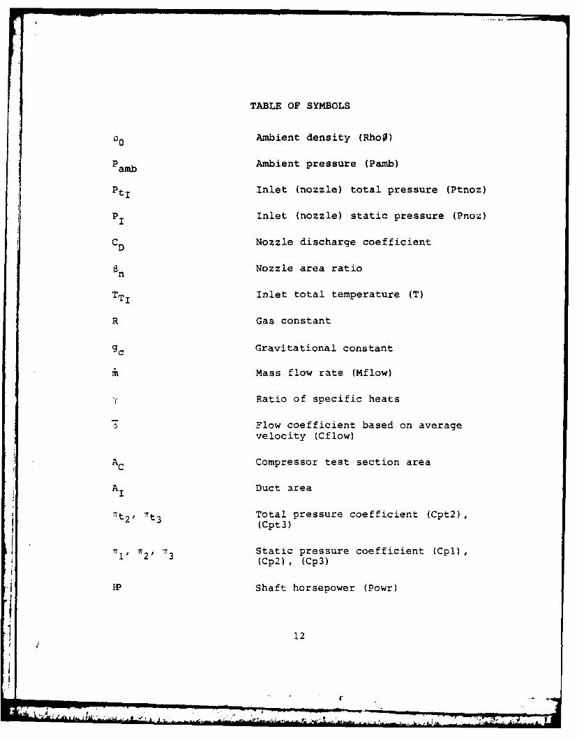
TABLE OF SYMBOLS
PO Ambient density (Rho0)
Pamb Ambient pressure (Pamb)
Pt, Inlet (nozzle) total pressure (Ptnoz)
P I Inlet (nozzle) static pressure (Pnoz)
CD Nozzle discharge coefficient
an Nozzle area ratio
TTI Inlet total temperature (T)
R Gas constant
gc Gravitational constant
m Mass flow rate (Mflow)
-I' Ratio of specific heats
7Flow coefficient based on averagevelocity (Cflow)
AC Compressor test section area
AI Duct area
7t2' 7t3 Total pressure coefficient (Cpt2),(Cpt3)
T1' T2 I3 Static pressure coefficient (Cpl),(Cp2), (Cp3)
IP Shaft horsepower (Powr)
12

Rpm Rotational velocity (Rpm)
Tq Shaft torque (Torq)
X Work coefficient (Cwork)
n t Average total-to-total efficiency(Etaav)
I' 2' 3 Respective probe flow pitch angles(Phi)
al' a2 ' a3 Respective probe yaw angles (Alfa)
V1 , V2, V3 Absolute velocities
W1 , W2 Velocities relative to rotor
Bit $2 Flow angles relative to rotor (Beta)
VUl, Vu2 Circumferential velocity components
Val, Va2, Va3 Axial velocity components
Um Mean radius wheel speed
R Mean radiusm
Si, S2, S3, S4, S5 Throttle screen elements
Note: Names in parentheses are those used in the HP 9845Asoftware.
Units are defined in the text as needed and in tablesof results.
13
ACKNOWLEDGMENT
I wish to express my sincere appreciation to the entire
Turbopropulsion Laboratory staff for their assistance, en-
couragement and patience. Without the benefit of their ex-
perience and ingenuity many of the steps in this program
could not have been completed. My thanks go to Dr. R. P.
Shreeve for his direction and his help in putting it all
together. I especially thank Mr. Jim Hammer for his constant
encouragement and support, for the questions he answered, and
for the questions he asked.
14
-- -- o . . . . . . r . .

I. INTRODUCTION
Secondary flow effects and associated losses that result
from finite tip clearances in compressors are not fully un-
derstood. The low speed axial flow compressor at the Turbo-
propulsion Laboratory of the Naval Postgraduate School is
currently being used to improve understanding of the tip
clearance problem and to generate better prediction methods
for the effects. To this end, the axial compressor was re-
configured as described in Ref. 1 to facilitate new experi-
mental studies. The redesign was intended to:
1) provide an axisymmetric flow as uniform as possibleahead of the compressor;
2) provide a means to determine accurately the mass flowrate;
3) allow an easy adjustment of the mass flow rate;
4) minimize the pressure losses at open throttle to pro-vide the maximum range of mass flow rate.
In this configuration, Welch performed preliminary tests
with solid body blading, as reported in Ref. 2. Symmetric
blading was selected for the tip clearance investigation
and new blading was designed and reported in Ref. 3. Ini-
tial tests with one stage of the new symmetric blading were
made by Moyle but were terminated by an accidental failure
which resulted in a total loss of the blading and some in-
strumentation. Results from these tests, referred to as
15
Build 1, were reported in Ref. 4. A new set of inlet guide
vanes was cast, as detailed in Ref. 5, and the compressor
was rebuilt with one stage. This configuration is desig-
nated Build 2.
The purpose of the present investigation was to evaluate
the current Build 2 and to determine its suitability for
studies of tip clearance effects. In the course of the work
the performance of individual blade rows as well as the over-
all compressor performance were examined, measurements were
refined where problems were encountered, and the flow fields
were examined throughout the stage.
16
AtI

II. APPARATUS
A. COMPRESSOR TEST RIG
The low speed axial flow compressor was designed to pro-
vide a large enough scale to allow the insertion of multiple
intrastage sensors without altering the flow fields. The
three foot diameter compressor, shown in Fig. 1, is capable
of one to three stages of operation. When less than three
stages are used, the stages may be built up in a normal
closely spaced configuration or in an expanded configuration
with wide separation between stages or between blade rows of
a given stage. There are thirty rotor blades and thirty-two
stator vanes per stage and each stage is identical. One
row of thirty-two inlet guide vanes and one or two rows of
thirty-two exit guide vanes may be installed. For the pres-
ent measurements, one stage of symmetrical blading was in-
stalled in a closely spaced configuration with one row of
inlet guide vanes and one row of exit guide vanes. The ac-
cess ports in the case-wall are arranged in eight axial lo-
cations and allow insertion of intrastage probes at various
peripheral locations relative to the fixed blading. The
survey planes are shown in Figs. 2 and 3. Provisions are
made for mounting a traverse rig which allows for circum-
ferential as well as radial surveys in any of six locations.
The traverse unit, shown in Fig. 3d, was mounted in the
11
L I
first access location. Additional sensors may be installed
by drilling the test section casing or duct walls.
Flow enters the compressor from outside the laboratory
through a twenty-one foot long duct which contains a throt-
tling device. A choice of two inlet bellmouths, used to
meter the flow rate, attaches to the front of the ducting
and is surrounded by a protective screen enclosure. The
large inlet bellmouth with a three foot throat diameter is
used for conditions where minimum pressure drop is desired.
The smaller 2.1 foot throat diameter bellmouth is used when
a greater pressure drop can be accepted. The duct has a
section which can be removed, when the large bellmouth is
used, to reduce the boundary layer growth. Only the large
bellmouth was used here, but the duct section was not re-
moved. Throttling is accomplished, as described in Ref. 6,
by the insertion of screens or perforated plates into the
inlet flow causing a drop in total pressure. Throttling
is therefore fixed for each run and may be changed only by
stopping the compressor. Flow exits the compressor and is
vented into the building via a conical diffuser.
The compressor is driven by a constant speed electric
motor, rated at 150 horsepower, and is coupled to the com-
pressor by ten drive belts. The drive ratio can be changed
by changing the drive sheaves, allowing operation at nomi-
nally 1588, 1818 and 2290 revolutions per minute. With the
low speed drive sheave installed the compressor was operating
19

at roughly 1616 RPM for all tests reported in the present
work.
B. DATA ACQUISITION SYSTEM
Data was acquired using the Hewlett Packard HP 3052 Data
Acquisition controlled by an HP 9845A computer. The system
included a HP 34495A Scanner, HP 3495 Digital Volt Meter
(DVM), HG 78K Scanivalve Controller and signal preprocessor
circuits. The HG 78K Scanivalve Controller (manufactured
in-house) controlled the two solenoid driven 48 port Scani-
valves. Each Scanivalve, referred to ambient pressure,
provided the ability to read 48 pressures with a single
transducer. All data were recorded by the computer via the
scanner, the digital volt meter and interface bus.
Data acquisition was accomplished using the "GENUSE",
general acquisition program, described in Ref. 7. Briefly,
the program controls the reading of data from up to five
Scanivalves and 35 other channels, stores the data on tape
and gives a tabulated printed copy. Two modifications were
made to the program. An on-line reduction routine was added
and a change was made in the non-Scanivalve data reading
subroutine to allow a torque reading to be made which was
averaged over an extended time.
C. INSTRUMENTATION
The instrumentation consisted of numerous pressure sen-
sors and several other non-pressure devices. The pressure
19
- *|

sensors included three United Sensor five hole probes, two
total pressure rakes, four Kiel probes, a simple total pres-
sure probe, twelve static pressure taps, and an ambient
pressure sensor. For some tests a cobra probe and a yaw
probe were added. The non-pressure devices included three
thermocouples, a torquemeter, a tachometer, and six linear
potentiometers to record radial and angular positions of the
movable probes. Table 1 lists the quantities measured.
Where possible, the pressure sensors were connected to one
of the Scanivalves because of the ability to do an on-line
scale verification. This was donk' by connecting Scanivalve
port one to the transducer reference pressure (atmos) to
give the zero reading (or tare) for the transducer while
the second port was connected to a manometer column pres-
surized to a controlled pressure in inches of water. This
allowed the scale factor and zero drift to be checked at
each data point. Two dedicated transducers were used to
measure the bellmouth pressure drop and ambient pressure.
The electrical signals from all transducers were conditioned
before digitizing by the digital volt meter. Each Scani-
valve and non-Scanivalve channel incorporated a signal con-
ditioning circuit to allow the zero point and scale factors
to be set.
Ambient pressure within the building was measured using
an absolute pressure transducer. Verification readings were
made periodically using a Fortin type barometer. Excessive
20

drift in the absolute transducer generally led to the use of
the barometer readings in all calculations. Ambient tempera-
ture was sensed using two "J" type thermocouples in the inlet
duct with an electrical equivalent ice point reference. The
recovery factor of the thermocouples was taken to be unity.
Total temperature rise was measured differentially by aver-
aging the outputs of two "J" type thermocouples located at
mid-radius at the stator exit and connecting them in series
with the thermocouples in the inlet. The rotational speed
of the compressor was measured using a magnetic pickup con-
nected to a digital counter. The signal was read manually
using a multimeter (although provisions exist for automatic
reading through the scanner). Torque was measured using a
Lebow Model 1215-6K torquemeter which was statically cali-
brated periodically between tests. The stability of the
torque calibration was verified using an electrical shunt
prior to each run. Inlet bellmouth (nozzle) pressure drop
was measured using a differential transducer between the
pressure (stagnation) within the inlet enclosure and the
pressure (static) in the nozzle throat. The two pressures
were also measured individually using two adjacent ports on
the first Scanivalve. The Scanivalve measurements were used
for all calculations since the drift of the dedicated trans-
ducer could not be checked over long run periods. One port
of the first Scanivalve was connected to a total pressure
tube inside the duct at a distance of two duct diameters
21
- J . . . .

downstream of the throttle. This reading was used purely
for verification of other readings and was not used for
calculations. The test section inlet total pressure was
measured using a twelve hole rake at survey plane one.
Total pressure was determined using a mass averaging tech-
nique described in Appendix D. The exit total pressure was
measured using a similar rake, applying the same mass aver-
aging technique. Eight case wall static pressure taps,
corresponding to the eight survey planes and two hub static
pressure taps were used. Four Kiel probes at mid-radius at
the stator exit completed the instrumentation on the first
Scanivalve.
The second Scanivalve was used for the three United Sen-
sor five hole probes, and the total pressure on the cobra
probe, when it was used. The survey probes, described in
Appendix A, provided measurements of yaw, pitch and velocity
magnitude at survey plane two (station 1), survey plane
three (station 2) and survey plane four (station 3). The
radial positions and yaw angles for the probes were recorded
from linear potentiometers attached to the probe mounts.
For the station 3 probe in the traverse unit, readings were
recorded from potentiometers set manually from the digital
counters in the traverse unit. A similar technique was used
for the cobra probe. The five hole probes were yaw-balanced
using a forty-five degree inclined manometer board. Ac-
curate measurements required that the balancing be done very
22
r . . , .. . q
4 . ..

carefully. In shear layers or turbulent flows, the diffi-
culty involved in yaw-balancing added to the uncertainty in
the probe measurements.
I
[t
2.3
' 2- A -19L

III. TEST PROGRAM AND RESULTS
A. SUMMARY
The test program was carried out in three phases. First,
a performance map was taken and limited flow field surveys
were made. The results from these tests appear in Tables 3
to 8 and Figs. 4 to 8. Second, the inlet guide vanes were
adjusted to three different settings to alter the flow angles
into the rotor. The results from these tests appear in Ta-
bles 9 to 31 and Figs. 9 to 34 and include both performance
maps and surveys made near the observed peak efficiency.
Third, the inlet guide vanes were returned to the original
configuration and surveys were taken at and near the peak
efficiency and at two well-off-design throttling conditions.
The results from these tests appear in Tables 32 to 40 and
Figs. 35 to 47. Other supplemental tests taken concurrently
with the other testing include examining fluctuations in
torque and flow rate, nozzle flow rate verification, and a
comparison of probe results obtained in peripherally dis-
placed survey holes to examine axisymmetry.
B. PHASE 1
The first phase performance map involved twenty-two
throttle conditions from fully open throttle through all
possible combinations of the screen-type throttle elements.
24

The three survey probes remained at mid-radius where the flow
vectors were determined (Table 4). This is the configuration
in which build one data was available for comparison. The
performance parameters are listed in Table 3 and plotted in
Fig. 4. Comparisons with build one data and the design pre-
dictions appear in Fig. 5. Note that the build one data re-
flects only the mid-span pressure rise and not a spanwise
integrated value. The pressure rise was virtually linear
with flow rate, never showing a peak but indicating a change
in slope at very high throttling. The power and the effi-
ciency both showed a definite rise and fall but the peak
values, occurring at a flow rate of roughly ¢ = .76, were
obscured due to 2% fluctuations in the torque measurement.
The pressure ratio through the stage varied from 1.014 to
1.02.
The flow angle at the inlet guide vane exit (station 1)
remained essentially constant through the measured range of
flow rates at 17.5 degrees as is plotted in Fig. 6. The
mid-span rotor exit angle (station 2) varied nearly linearly
with flow rate. The flow angle at station 1 was 3.8 degrees
less than the design prediction. A less detailed performance
map was taken with the probes at seventeen inches radius.
The guide vane exit angle exhibited even more severe under-
turning than at the mid-radius with the measured angle vary-
ing one degree from 23 to 22 degrees (Fig. 7). Limited
surveys taken while examining the axisymmetry of the flow
25
indicated that these angles were quite typical of the condi-
tion in the blade-to-blade direction.
Radial flows were noted at all stations. At station 1,
there was a consistently inward flow which was most severe atI low throttling. At station 2, the radial component shifted
from radially outward at low throttling to inward at high
throttling. The opposite occurred at station 3. As can be
seen in Fig. 7, the station 3 probe showed a relatively con-
stant yaw angle as the flow was throttled initially, but the
yaw angle increased rapidly below a flow rate of =0.75.
C. PHASE 2
To "force" the rotor inflow angle to match the design
angle at mid-span, the inlet guide vanes were turned four
degrees counterclockwise. This resulted in a large reduc-
tion in flow rate, pressure rise, and power required, varying
from 5.4 to 3.1 percent (Table 8). This came from "unload-
ing" the rotor as the requirement for turning was reduced.
The efficiency was significantly reduced at high flow rates
but changed little at the moderate and low flow rates (Fig.
9). The flow angles out of the inlet guide vanes at mid-
span were closer to design as shown in Fig. 10. However
Fig. 12 shows that the guide vane exit flow was still under-
turning at the outer radii, and now overturning at the inner
radii. The angles at station I. had shifted uniformly across*1 the radius in the direction the guide vanes had been turned.
26
-. f &

Also, although the inlet flow angles were somewhat improved,
the stator exit angles were not correct for any succeeding
stages. The radial flows were altered noticeably. The flow
at station 1 showed a minimum inward component near the
"maximum" efficiency (Table 9). The flow at station 2 was
consistently inward, being somewhat less so away from the
peak efficiency condition. The stator exit flow was outward
near peak efficiency and inward at lower or higher throttle
conditions.
Total and static pressure distributions, taken from the
survey probes, showed that the static pressure rise was about
equally divided between the rotor and the stator (Fig. 15).
The rise was greater at the tip but relatively flat overall.
The total pressure rise across the rotor was skewed slightly
toward the tip. The overall stage total pressure rise can
not be inferred from the data in Fig. 14 since the probe was
at a single peripheral position well clear of the stator
wakes.
The inlet guide vanes were adjusted back one degree
clockwise to be three degrees from the original configura-
tion. The performance, shown in Fig. 16, was found to be
similar to that obtained at the four degree setting. How-
ever, there were indications of a possible upturn in the ef-
ficiency with increased throttling at the lowest flow rate
after an apparent peak efficiency at a flow rate of about
= .73 compared to results at the 40 guide vane setting.
27
2 1 , " ,° * -

The pressure rise at peak efficiency increased by 4 percent,
at low throttling by 2 percent and at highest throttling by
1 percent (Table 12) . Shown in Fig. 17, the flow angles at
stations 2 and 3 showed similar trends to those measured at
the four degree setting. The stator exit radial flow showed
a distinct trend from inward at low throttling to outward at
high throttling (Table 13).
Several surveys were taken near the peak efficiency.
These surveys, concentrated in the hub and tip regions,
showed a reversal in flow angle at both the hub and tip.
This was true at all three stations. The surveys also showed
that the rotor total pressure rise was still slanted toward
the outer radii, even slightly below the observed peak per-
formance. The through-flow velocities were also higher at
the outer regions, corresponding to regions of greater pres-
sure rise (Fig. 21). Surveys were taken at locations dis-
placed circumferentially relative to the inlet guide vanes.
The results shown in Fig. 48 show that the flow angles were
much better behaved toward the pressure side of the blade
and roughly the same near mid-passage or toward the suction
side. The pressure side showed slightly lower velocities
and had a much lower radial flow (Table 30).
The inlet guide vane angle was reduced by one additional
degree to give a stagger angle two degrees greater than in
the original configuration. The performance map was re-I peated and several surveys were taken. At this point, the
28
......................................M

acquisition program was changed to read the torque over a
longer period which yielded a more stable reading. The re-
sults in Fig. 23 show that the performance again yielded an
indistinct peak in the efficiency. In fact, the efficiency
appeared to rise again at the highest throttling to the pre-
vious peak value. The pressure rise and power required
showed no different trends, being similar to the original
configuration. The radial flow components also showed
similar trends (Table 19).
During the surveys, a lack of stability was noted in the
flow angles at station 1 at radii between sixteen and seven-
teen and a half inches. The flow angle would remain steady
for several seconds, then drift to a new value (Fig. 33).
The flow appeared to vascillate about an intermediate value
that followed a smooth variation as a function of radius.
Repeating the survey, using a two tube yaw head probe, the
vascillations were not apparent and the flow angles did fol-
low a smooth curve (Fig. 34). With the smaller yaw probe,
angles were measured very close to the outer wall. The re-
sults showed a strong reversal in the flow angle at the tip
at all three stations.
D. PHASE 3
The inlet guide vanes were returned to the original con-
figuration and three surveys were taken with moderate throt-
tling and one was taken at very low (Figs. 40-43) and one at
29
- .__ >4.

very high throttling (Figs. 44-47). These surveys showed the
changes in the flow fields over the range of flow rates. As
throttling was increased, the flow rate decreased and the
pressure rise shifted from being greatest at the hub to being
j greater at the tip. The ill-defined peak efficiency occurred
when the distribution in pressure rise was approximately uni-
form across the blade height. The off-design inlet conditions
caused the peak to occur at a flow rate slightly lower than
f or uniform pressure rise when the bulk of the work and flow
rate were concentrated at the outer radii. At the low flow
rates the pressure field was the most distorted and the ra-
dial components of the velocity were the greatest.
E. SUPPLEMENTAL TESTS
Supplemental tests were conducted during the program to
examine three areas. These tests looked at flow rate and
torque fluctuations, nozzle flow rate verification, and com-
parison of results from different peripheral survey locations
to examine axisyinmetry. The results of these tests appear in
Figs. 48 to 51.
Output from the torquemeter and nozzle pressure drop
transducer were connected to oscillographs and continuous
readings were taken. As seen in Fig. 51, the torque fluc-
tuations were typically plus or minus 15 inch-pounds with a
frequency of consistently 5.5 per second. with a compres-
j sor speed of 1616 RPM, this was one oscillation per 4.9
30
7A 7
revolutions of the drive motor running at 1180 RPM. The
nozzle pressure fluctuations had a frequency of three per
second. Thus the torque fluctuation varied at a rate of 1.8
oscillations per flow rate oscillation. The amplitude of
the nozzle pressure drop variations was unsteady in time and
no wave form analysis was done to look for frequency content.
An attempt was made to verify the flow rate measurements,
in an approximate way, since an integration of radial probe
surveys downstream of the rotor had suggested that the flow
rate should be somewhat higher than was measured. The flow
at tne inlet to the compressor (survey plane 1) was traversed
using a cobra probe and the total pressure distribution was
recorded (Fig. 50). Assuming axisymmetry and constant static
pressure at the value measured at the wall, the mass flux
distribution was calculated and integrated to obtain the
total flow rate. The result was found to correspond to the
use of a discharge coefficient for the large bellmouth of
1.026, rather than 0.98 which had been used to date. This
higher value was used in all calculations.
The degree of axisymmetry was examined by moving the
survey probes and rakes to various survey ports about the
circumference. At survey plane one, rakes were placed in
four of the nine ports and good agreement was obtained in
the results. Similarly, ports five, seven and nine showed
good agreement at survey plane two. The stator exit was
surveyed circumferentially at three radii (Fig. 49). The
31
wake was consistently centered at 90 on the traverse unit at
all three radii at moderate throttling. Thus the flow mea-
sured at station 3 was clear of the wake for all other runs
for which the probe was typically located at the 51 position.
The exit rake was moved to 5 ports at 3 survey planes between
the stator and exit guide vanes. The locations furthest aft
of the stage allowed the best mixing of stator wakes but also
reflected the build-up of hub and case wall boundary layers.
32
... , , ,. . .,E..4A

IV. DISCUSSION
A. FLOW FROM THE INLET GUIDE VANES
The most significant result from the measurement program
was the behavior of the flow angle from the inlet guide
vanes. The significant underturning at the outer radii re-
lated directly to the alteration of the performance of the
compressor. This underturning, roughly ten degrees at 17.5
inches radius and four degrees at mid-radius, required the
rotor to do increased work as compared to the design and led
to a violation of the radial equilibrium condition. The
result was to change the pressure distributions and flow
rates through the machine. Comparison with build one showed
that the flow angle at mid span was 20 greater in build one,
suggesting that there should be a difference in performance
in the two builds, and thi~s was observed. Vascillations in
flow angle at the outer radii indicated the possibility of
the presence of a flow separation. Since these problems af-
fected the performance of the rest of the compressor, any
discussion must begin with the inlet guide vanes.
As discussed in Ref. 8 and Ref. 9, secondary flows result
when boundary layers pass through a set of stationary turning
vanes. In particular, the fluid particles within the case
and hub wali boundary layers tend to move toward the convex
side of the flow passage and roll up into two trailing
33
*. . . . . . .. . .. ... t77

vortices moving downstream. Modeling of this effect using
small perturbation theory predicts that there will be over-
turning within the boundary layer and underturning outside
of it. Reference 9 indicates that this is well supported
by experimental experience in rectilinear (2D) cascades and
that the underturning may be seen in the flow at a distance
of three or four boundary layer thicknesses. The compressor
is not two dimensional and is imposing on the flow a radial
gradient in axial velocity and static pressure. While these
are not the conditions as described in Ref. 9, the effect
should be similar. With the case wall boundary layer being
roughly one inch at moderate throttling, this effect could
be expected to be seen inwards towards or even past the mid-
radius. The hub boundary layer, with a thickness of about
two tenths of an inch, has a much smaller and only local ef-
fect. It does however exhibit the same underturning/over-
turning pattern.
The differences in radial flow component shown in Table
30 tend to support this explanation of the mechanisi caqs-
ing the distorted flow at the guide vane exit. Along the
pressure side of the vane, in the outer regions the calcu-
lated pitch angle is the most strongly positive. It de-
creases across the passage as measured in survey ports 7 and
8. Because the pressure taps on the probe are separated
radially, the indicated pitch angle in a pressure gradient
can be in error as a result of the gradient. Thus an
34
~ I I I -, - . L.
alternative explanation for the differences in pitch angle
is that the radial pressure gradient is steeper along the
pressure side of the blade. The hub region exhibits a
similar behavior to that described for the outer regions
but of smaller magnitude. The shape of the curves in Fig.
48 at the three survey locations support the idea of second-
ary flows as the cause of underturning since the angles
measured away from the vane wakes qualitatively match
closely the pattern predicted in Ref. 9. Note that the flow
angles at mid-span were closer to the design values in build
one than in build two (until the IGV's were adjusted). Thus
there is an additional mechanism for underturning in build
two in addition to the secondary flow effects discussed
here.
Vavra indicates in Ref. 10 that the flow at the exit of a
set of guide vanes is very sensitive to the distance a be-
tween neighboring blades as defined in Fig. 52. The relation-
ship between passage exit area, blade spacing and efflux
angle (at the mean line conditions) is approximated in Ref.
10 by the relationship e = cos - 1(a/s)( +te)(i - C s - (a/s )e s 90
The angle will decrease for either an increase in trailing
edge thickness or an increase in the distance a for constant
spacing. The trailing edge thicknesses are reported in Ref.
11 to be thicker for build two than for build one. For the
additional underturning to be solely due to the larger trail-
ing edge thickness it would require even larger thicknesses
35
r
than were reported. For a to be larger for the build two
blades, the blade thickness would need to be smaller, which
was not the case, or the blades would have to have been made
with a shorter chord, which is known to be true for some
blades. Therefore a combination of thicker trailing edges
and shorter chord blades is probably the cause for the addi-
tional underturning seen in build two as compared to build
one. one possibility for narrower blades would be excessive
trimming during the removal of the flashing from the casting
process. Another would be shrinkage of the epoxy after
moulding but this is considered less likely, since most
epoxy materials are known to swell slightly due to the dif-
fusion of water molecules into the material.
Reynolds number effects must also be considered as a
possible cause for the general level of underturning. Below
a Reynolds number of 2.2 x 10O5, a decrease in deflection
angle could be expected. At moderate throttling the Rey-
nolds number based on mid-span chord was approximately
2.5 x 10~ at the most closed throttle condition. Since the
guide vane exit angle was essentially constant over the
operating flow range, Reyniolds number effect appeared to be
minimal. The stator exit angle changed appreciably at the
lower flow rates but this was probably the result of in-
creased incidence angles from the rotor rather than an ef-
fect of Reynolds number.
26
The presence of a peripheral gradient across the pas-
sage could cause an error in yaw angle measurement in view
of the separation of the yaw ports in the probe. This was
discounted after measurements were made with a yaw probe
which had its ports mounted along the same radial line, and
similar results were obtained.
The erratic yaw angles experienced on some tests sug-
gested the presence of a flow separation along the suction
side of the guide vanes. Should the flow be separated, the
flow angles would be expected to be reduced. Consistent
with this observation, the flow closest to the pressure side
of the blade demonstrated less underturning than at the two
locations toward the center of the passage. The frequency
of the change in the flow angle that occurred after the
probe was balanced did not correlate with any of the mea-
sured flow rate oscillations or the typical one half per
rotor revolution frequency of a rotating stall. It was
clearly an intermittent rather than a periodic condition.
It is possible therefore that the flow detaches and reat-
taches intermittently and further measurements are required
to define the process clearly.
B. PERFORMANCE DIFFERENCES
The measured performance departed from the design expec-
tation, shown in Fig. 5. Several factors could have contri-
buted to the differences. For example, the design was
37
! !
carried out for a single stage operating speed of 2290 RPM
whereas the present tests were limited to 1616 RPM. Thus
there was a possibility of a small Reynolds number effect
on the performance as described in Ref. 8. Secondly, the
test rig was intended to be run with the first six-foot sec-
tion of duct removed in tests witlP the large inlet bell-
mouth. The extra length would have contributed a small
amount to the boundary layer growth. Clearly, however,
these differences are minor in comparison with the likely
effect of the underturning of the guide vanes.
Comparisons with build one showed a rise in power, and
flow rate in build two. The two degree shift in the rotor
inflow angle caused greater loading on the rotor yielding
a higher pressure rise and work requirement. The power in-
creased roughly two percent over build one with an increase
in flow rate of about 1.5 percent. The pressure rise within
the stage was altered appreciably. At mid-span, the static
pressure rise shifted more to the rotor; but at the case
wall the static pressure rise, as measured by the wall static
ports, shifted more toward the stator. No surveys were
available from build one to allow a comparison at other
radial locations, but the limited data did suggest a sig-
nificant alteration in the internal flow fields. Further
differences were in the radial flows at station two and
three which showed much sA.,aller magnitudes in build one.
38
~r~r7~ 27

It was extremely difficult to determine the peak effi-
ciency for several reasons. First, the performance charac-
teristic, which resulted from the incorrect flow fields, was
very flat. The fluctuations occurring in the pressure rise
and torque compounded the problem. With high flow volumes
undergoing only slight pressure rises the work input could
be greatly affected by perturbations in the torque or in the
nozzle flow rate. Also, the radial exit total pressure rake,
situated well aft of the stage, was influenced by the case
wall and hub boundary layers and did not fully average the
flow from the stators. This generated an uncertainty as to
the true variation in the mass-averaged total pressure rise
with flow rate.
C. MEASUREMENT UNSTEADINESS
The flow rate and torque fluctuations were apparently
not related to any structural or flow feature of the machine.
The frequency of the fluctuations did not correlate with
each other nor with the (approximately) one per two revolu-
tions of a rotating stall. Nor did they correspond to har-
monics of the drive motor which operated at 1180 revolutions
per minute. They were not similar to the natural frequen-
cies of the blades given in Ref. 5. The flow vascillations
observed at the outer radius occurred with a period esti-
mated to be ten seconds or longer; torque and flow fluctua-
tions were much more rapid. One possible explanation for
39
!4
the torque fluctuations is that they were a result of play
in the drive belts, but no means were available to examine
the connection. Thus, there was no evidence that the torque
fluctuations produced corresponding fluctuations in the flow
fields, and they were accepted as an undesirable contributor
to uncertainty in the measurement of efficiency.
40
I~
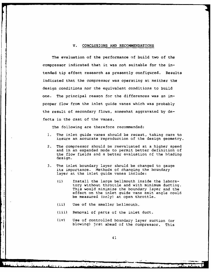
V. CONCLUSIONS AND RECOMMENDATIONS
The evaluation of the performance of build two of the
compressor indicated that it was not suitable for the in-
tended tip effect research as presently configured. Results
indicated that the compressor was operating at neither the
design conditions nor the equivalent conditions to build
one. The principal reason for the differences was an im-
proper flow from the inlet guide vanes which was probably
the result of secondary flows, somewhat aggravated by de-
fects in the cast of the vanes.
The following are therefore recommended:
1. The inlet guide vanes should be recast, taking care toinsure an accurate reproduction of the design geometry.
2. The compressor should be reevaluated at a higher speedand in an expanded mode to permit better definition ofthe flow fields and a better evaluation of the bladingdesign.
3. The inlet boundary layer should be changed to gaugeits importance. Methods of changing the boundarylayer at the inlet guide vanes include:
(i) Install the large bellmouth inside the labora-tory without throttle and with minimum ducting.This would minimize the boundary layer and theeffect on the inlet guide vane exit angle couldbe measured (only) at open throttle.
(ii) Use of the smaller bellmouth.
(iii) Removal of parts of the inlet duct.
(iv) Use of controlled boundary layer suction (orblowing) just ahead of the compressor. This
41
no

would probably be desirable in the course of
the tip clearance investigation to follow.
The logical procedure is to first carry out 3(i) without
compressor geometry changes to answer definitively whether
secondary flows developing from case wall boundary layer are
the primary cause of the observed underturning. Depending
on the results of this first test, either new inlet guide
vanes should be cast or a new design should be developed
which accounts properly for deviation angle in the presence
of radial gradients in through flow.
42
r - "-

Table 1. Measured Quantities, Typical Set-up
S.V. #4 S.V. #4 (Cont'd) S.V. #4 (Cont'd)
PA - PA Inlet Rake P 17.00-P A Exit P t3-3 - PA
Pcal -P A Inlet Rake P 17 .50-PA Exit Pt3-4 - PAp PA Inlet Rake P 17.75-P A Exit Rake P 11.00-P tP noz
P2noz -PA SP-1 PHub - PA Exit Rake Pt11.50-Pt
p - PA SP-1 PTip - PA Exit Rake Pt2.00-PPtpipe ATp Att
Pspipe - PA SP-2 PTip - PA Exit Rake P t12.75-Pt
Inlet Rake Pt11.00-PA SP-3 PTip - PA Exit Rake Pt 13.50-P t
Inlet Rake P 11.50-P SP-4 P - P Exit Rake P 14.40-Pt A Tip A t t
Inlet Rake Pt1 2.0 0-PA SP-5 PTip - PA Exit Rake Pt 15.30-Pt
Inlet Rake Pt2.75-PA SP-6 PTip - PA Exit Rake Pt6.00-Pt
Inlet Rake Pt3.50-PA SP-7 PTip - PA Exit Rake Pt6.50-Pt
Inlet Rake Pt14.40-PA SP-8 PTip - PA Exit Rake Pt 17.00-Pt
Inlet Rake Pt 1.30-PA SP-8 PHub - PA Exit Rake Pt17.50-Pt
Inlet Rake Pt16.00-PA Exit Pt3-1 - PA Exit Rake Pt 17.75-P t
Inlet Rake P1t6.50-PA Exit P t3-2 - PA
S.V. #5 Scanner #1
PA PA Tt0 - "J" - IPR
Pcal- PA AT out i
Probe "X" P - PA AT out 2
Probe "X" - PA NT Brg. Front
Probe "X" P4 - PA AT Brg. Rear
Probe "X" P5 - PA RPM - F/V
Probe "Y" P - PA PBaro "Hg Abs
Probe "Y" P2 3 - PA APProbe "Y" P - P Torque--in-lbs
4 AProbe "Y" P - P Probe "X"--Pos5 AProbe "Z" P 1- P A Probe "X"--Yaw
Probe "" P - P Probe "Y"--PosP23 A
Probe "Z" P4 - PA Probe 'Y"--Yaw
Probe "2" P5 - P A Probe "Z"--Pos
Probe "Z"--Yaw
43
,-c
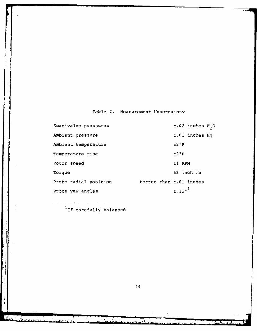
Table 2. Measurement Uncertainty
Scanivalve pressures ±.02 inches H20
Ambient pressure ±.01 inches Hg
Ambient temperature ±20F
Temperature rise ±20 F
Rotor speed ±1 RPM
Torque ±2 inch lb
Probe radial position better than ±.01 inches
Probe yaw angles ±.250
I1f carefully balanced
44
... ., ... . * . . . . " ... % i - , ;"" A ' >" I -. .... .

Table 3. Performance Parameters (IGVs 0)
I Cilow POWER Cwork CpZ3 Etaav Etats T T3-T Prise1 .9888 50.697 .6376 .5566 .9730 .1042 65.81 -.13 1.013
..9899 50.745 .6386 .5312 .8318 .0670 66.73 -.78 1.0123 .9366 51.085 .6417 .5527 .8612 .1026 64.07 -.07 1.0134 .9510 52.679 .6880 .5965 .8671 .2214 65.15 1.26 1.6145 .956? 53.343 .6926 .5844 .8438 .1914 65.24 2.15 1.0136 .9566 53.016 .6899 .5954 .8630 .2160 65.97 .96 1.6147 .9221 53.460 .7218 .6310 .8742 .2881 66.42 1.52 1.8148 .9283 54.056 .7239 .6336 .8743 .2909 65.66 1.56 1.0159 .9249 54.367 .7317 .6332 .8654 .3034 66.34 .95 1.01510 .8907 54.800 .7664 .6760 .8742 .3861 66.72 1.33 1.01511 .915 56.019 .7815 .6793 .8692 .3793 65.90 1.86 1.01612 .9922 55.750 .7765 .6786 .8739 .3829 65.50 2.25 1.01613 .8554 55.206 .8063 .7241 .8980 .4607 68.26 .74 1.01714 .8536 56.066 .8171 .7219 .835 .4519 66.06 2.05 1.01715 .3537 55.196 .8055 .7173 .8911 .4574 66.33 .91 1.01716 .8362 55.739 .8311 .7458 .a974 .4918 67.17 2.12 1.01717 .3338 55.27 .3271 ."427 .8980 .4946 67.57 .96 1.01718 .8357 54.800 .8166 .7420 .9087 .4989 66.52 2.14 1.01719 •$880 54.800 .7685 .633: a:899 .3987 66..5 2.14 1.01620 .8830 55.032 .7745 .6767 .8737 .3850 65.50 2.71 1.01621 .3881 54.879 .7696 .6781 .8810 .:386 66.63 1.49 1.01622 .9811 56.541 8775 .7666 .87:36 .5156 65.68 1.78 1.01823 .8616 56.055 .8681 .7630 .87S9 .5176 64.93 2.2 1.01824 .3036 56.146 .9692 .7715 .8876 5236 66.08 2.00 1.01825 a30a7 55.302 .3677 .7692 .S865 53;30 63.40 1.02 1.1326 .a30:3 56,731 8767 .7669 ,743 .5175 64.92 1.71 1•81327 .8040 56.494 .8738 .7682 .8791 .5226 65.:37 1.18 1.01828 .7985 5 .334 .3725 .7393 .9047 5586 67.60 1.02 1. 01329 7963 56 .8 68 .3913 .7894 %8357 .5482 67.74 . 9 .015.30 .7975 !6.673 .38:32 7793 88'24 .520 65.50 11. 1. 01:331 7737 55.650 8901 7358 8823 5538 66.65 1. 44 11 332 7740 56.557 .9074 7863 .3665 .5400 65.07 1.74 1.01:33 7788 56.525 .9029 9 748 .5456 66.05 2.27 1:334 .715 56.055 .9061 .7987 a85 .5658 67.2 2.38 1.835 .7709 56.520 .9156 .3121 .8870 .5678 68.04 2.0 1.1936 .7730 56.736 .9147 .8021 S8770 .5639 66.94 1.30 1.01937 .755 56.130 .9284 .361'? .8637 .3558 6:8.:35 i.03 01:38 .7592 56.304 9269 .8074 .8710 .5606 6S.52 1.45 1.01?39 .7571 56.330 .9262 .8071 .8715 .55a4 66.:35 55 1.0194; .7546 56.172 .9250 .9147 .8807 57'9 65.33 2.' Z 1019
45
i ' ...-- "

Table 3 (Continued)
41 .7530 55.744 .9219 .8187 .S886 .5835 66.55 1.41 1.81942 .'526 55.876 .9266 .8137 .8782 .5752 67.73 2.7S 1.81943 .7342 56.140 .9498 .8273 .9711 .5837 65.23 1.76 1.019
44 .7345 56.071 .9473 .8243 .8761 .5815 64.68 3.37 1.01945 .1 55.856 .9441 .8261 .8751 .5855 66.13 2.62 1.81946 .7290 56.151 .9593 .3297 .8649 .5817 66.61 2.15 1.01947 .7341 56.168 .9539 .8383 .8765 .5848 67.68 1.46 1.81948 .7326 55.281 .9381 .8294 .a841 .5977 66.42 2.75 1.01949 .7314 55.586 .9416 .8319 .A835 .5986 63.85 2.63 1.019
50 .!333 56.383 .9526 .a336 .8751 .5909 63.89 3.23 1.01951 .7S48 55.882 .9473 .8339 .8798 .5977 66.99 2.00 I.1952 .7279 56.035 .9543 .8365 .3765 .5982 64.16 3.15 1.81953 .7292 55.a55 .9514 .S373 .88O1 .6036 65.28 2.46 1.01954 .7265 55.834 .955? .8385 .8774 .5975 65.81 1.37 1.01955 .700 55.581 .9708 .8372 .8624 .6084 62.8 2.05 1.02656 .7102 55.243 .9644 .8397 .8707 .6645 64.27 2.09 1.02057 .7119 55.802 .9730 .8425 .$659 .5992 64.a6 1.24 1.02653 .631 54.483 .9833 .850:3 .a647 .6133 65.86 1.40 1.02659 .6990 55.117 .9776 .8477 .8676 .6130 63.94 2.00 1.02060 .7011 54.151 .9591 .8521 .3884 .6258 65.06 2.1.3 1.02061 .6912 55.138 .9893 .8530 .8622 .6203 63.97 1.58 1.02062 .6941 54.958 .93828 .8560 .8717 .6211 64.43 2.51 1.02063 .666? 54.132 1.0964 .8492 .9438 62 13 6.3.30 2.60 1.02064 .6757 53.7 34 .9876 .3530 .8643 P-364 64.81 2.13 1.020
46
.. .. .... ... .
W 5,, t I d:
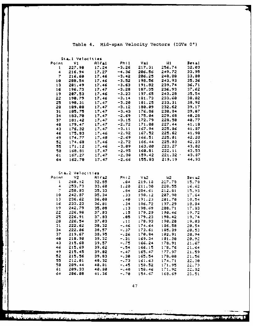
Table 4. Mid-span Velocity Vectors (IGVs 00)
Sta.l VelocitiesPoint VI RUal Phil Val w1 Betal
1 227.98 17.24 -3.26 217.31 256.74 32.034 216.94 17.27 -4.36 286.56 249.72 33.957 216.68 17.46 -3.42 286.25 248.88 33.88
18 208.54 17.46 -3.52 198.56 243.93 35.3613 201.49 17.46 -3.63 191.82 239.74 36.7116 196.73 17.47 -3.28 187.35 236.93 37.6219 207.53 17.46 -3.23 197.65 243.28 35.5422 198.79 17.46 -3.14 181.73 233.68 38.8225 190.31 17.47 -3.20 181.25 233.31 38.9228 189.08 17.47 -3.12 188.89 232.62 39.1731 185.75 17.47 -3.43 176.86 230.84 39.8734 183.70 17.47 -2.69 175.04 229.68 48.2837 181.42 17.47 -3.15 172.79 228.58 48.7748 179.47 17.47 -2.72 171.88 227.44 41.1843 176.32 17.47 -3.11 167.94 225.86 41.8746 175.83 17.46 -2.92 167.52 225.62 41.9849 174.77 17.48 -2.69 166.51 225.01 42.2052 174.68 17.46 -2.72 166.44 225.83 42.2355 171.12 17.46 -3.09 163.80 223.27 43.025a 168.81 17.47 -2.95 168.91 222.11 43.5361 167.27 17.47 -2.38 159.42 221.32 - 43.8764 162.78 17.47 -2.66 155.03 219.19 44.93
ta.2£ Velocities
Point V2 Rl&t2 Phi2 V12 W2 Betg,1 260. 2 32.85 .84 219.13 227.79 15.734 253.73 33.60 1.20 211.30 220.55
250.83 35.33 .84 204.61 212.81 15.9310 242.87 35.34 .33 198.12 287.90 17.6413 236.62 36.08 .48 191.23 201.70 18.5416 233.23 36.81 .34 186.72 197.29 13.8419 242.79 35.88 .13 198.69 288.71 17.3322 226.98 37.a3 .15 179.29 190.46 19.7225 226.91 37.83 .85 179.23 198.42 19.7428 226.54 37.83 .11 178.93 190.28 :9.8331 222.62 38.32 -.46 174.64 186.5e 20.5434 222.06 38.57 -.37 173.61 185.39 20.5237 219.67 38.95 -.26 178.94 182.91 20.9440 218.90 39.32 -.31 169.34 131.30 20.9243 215.68 39.57 -.75 166.24 178.91 21.6746 215.69 39.62 -.54 166.15 1-8.76 21.64
49 215.45 39.82 -.47 165.47 !77.97 21.5952 215.56 39.83 -.30 165.54 178.80 21.15655 212.81 48.32 -. 73 161.63 174.71 22.30
53 209.44 40.81 -.45 158.52 171.95 22.7961 289.33 40.88 -.40 158.46 171.92 22.8264 296.08 41.36 -.78 154.67 18.69 2S.51
47
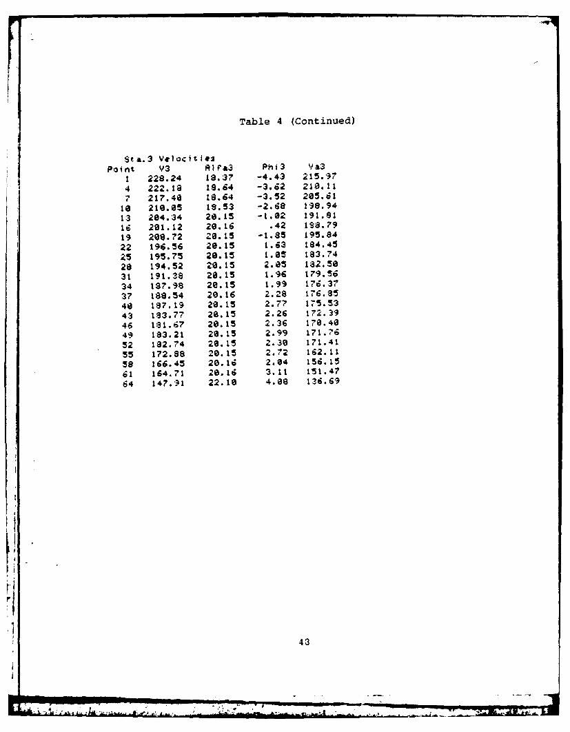
Table 4 (Continued)
Sta.3 VeIocitiEPoint V3 AIf'a3 Ph3 Va3
1 228.24 18.37 -4.43 215.97
4 222.18 19.64 -3.62 210.117 217.40 18.64 -3.52 205.61
10 210.05 19.53 -2.68 198.94
13 204.34 20.15 -1.02 191.81
16 201.12 20.16 .42 1S9.79
19 208.72 20.15 -1.85 195.84
22 196.56 20.15 1.63 184.45
25 195.75 20.15 1.05 183.74
28 194.52 20.15 2.05 182.50
31 191.38 20.15 1.96 179.56
34 187.98 20.15 1.99 176.37
37 188.54 20.16 2.28 176.85
40 187.19 20.15 2.77 175.5343 183.77 20.15 2.26 172.39
46 181.67 20.15 2.36 170.40
49 183.21 20.15 2.99 171.76
52 182.74 20.15 2.30 171.41
55 172.88 20.15 2.72 162.11
58 166.45 20.16 2.04 156.15
61 164.71 20.16 3.11 151.47
64 147.91 22.10 4.08 136.69
43
I '-.. -

Table 5. Mid-span Pressure Variationswith Throttling (IGVs 00)
Point P1 P2 P3 Pt1 Pt2 Pt31 -11.13 -9.94 -5.52 -.39 5.53 5.272 -11.80 -9.98 -5.52 -.22 5.54 5.053 -11.08 -9.87 -5.49 -.45 5.48 5.434 -11.18 -9.66 -5.22 -1.40 4.91 4.935 -11.24 -9.64 -5.21 -1.36 5.00 4.806 -11.28 -9.73 -5.23 -1.46 5.10 4.907 -11.25 -9.42 -5.02 -1.69 4.71 4.628 -11.28 -9.42 -4.99 -1.76 4.73 4.609 -11.20 -9.37 -4.95 -1.66 4.57 4.6618 -11.25 -8.92 -4.61 -2.48 4.29 4.3311 -11.29 -8.98 -4.59 -2.47 4.39 4.3112 -11.25 -8.95 -4.59 -2.45 4.28 4.3413 -11.24 -8.48 -4.24 -3.15 3.99 4.1914 -11.26 -8.49 -4.23 -3.21 4.06 4.1:315 -11.20 -9.45 -4.17 -3.14 3.94 4.1616 -11.25 -8.25 -4.00 -3.55 3.83 4.1617 -11.20 -8.22 -3.97 -3.50 3.84 4.1318 -11.22 -8.21 -3.98 -3.47 :3.84 4.1719 -11.23 -8.89 -4.53 -2.55 4.30 4.2320 -11.25 -8.92 -4.57 -2.55 4.29 4.2721 -11.29 -8.91 -4.54 -2.59 4.35 4.3222 -11.15 -7.81 -3.69 -3.91 3.62 4.1323 -11.21 -7.82 -3.72 -3.99 2.66 4.0524 -11.18 -7.81 -3.68 -3.89 3.67 4.1625 -11.13 -7.76 -3.63 -3.98 3.61 4.0826 -11.20 -7.04 -3.71 -:3.97 3.63 4.0827 -11.22 -7.35 -3.68 -:3.99 3.61 4.1428 -11.23 -7.75 -3.64 -4.16 3.5 3.9929 -11.14 -7.78 -3.54 -4.08 3.59 4.a930 -11.24 -7.76 -3.62 -4.25 ?.155 4.8131 -11.089 -7.40 -3.38 -4.26 3.52 4.0132 -11.09 -7.41 -3.36 -4.27 2.53 4.103:3 -11.09 -7.43 -3.32 -4.29 3.56 4.1634 -11.15 -7.38 -3.39 -4.48 3.44 3.6935 -11.11 -7.31 -3.27 -4.54 3.48 4.0136 -11.16 -7.39 -3.33 -4.43 3.48 3.9937 -10.?9 -7.15 -3.17 -4.52 3.43 3.9838 -18.98 -7.13 -3.18 -4.54 3.47 3 .9639 -11.03 -7.17 -3.17 -4.46 3.47 4.0340 -11.13 -7.17 -3.21 -4.76 3.37 3.86
49

Table 5 (Continued)
Point PI P2 P3 PtI Pt2 PT"341 -11.11 -7.15 -3.18 -4.68 3.39 3.8542 -11.12 -7.09 -3.11 -4.78 3.34 3.9243 -11.00 -6.89 -3.85 -4.86 3.32 3.7644 -10.97 -6.88 -3.87 -4.86 3.34 3.7245 -10.98 -6.39 -3.08 -4.83 3.34 3.7446 -10.98 -6.84 -3.13 -4.89 3.33 3.5047 -18.96 -6.86 -3.87 -4.86 3.30 3.6248 -10.95 -6.84 -3.02 -4.81 3.34 3.7649 -11.88 -6.92 -3.11 -5.02 .3.23 3.6650 -11.08 -6.89 -3.14 -5.80 3.33 3.5851 -11.07 -6.91 -3.09 -4.99 3.31 3.6652 -11.05 -6.88 -3.09 -5.01 3.32 3.6453 -11.06 -6.86 -3.09 -5.03 3.34 3.6154 -11.07 -6.89 -3.07 -5.05 3.28 3.6255 -10.95 -6.68 -3.07 -5.15 3.19 2.9656 -10.96 -6.68 -3.07 -5.16 3.18 3.8957 -10.95 -6.65 -3.03 -5.18 3.20 3.1258 -10.90 -6.51 -3.03 -5.29 3.87 2.5359 -10.39 -6.51 -3.08 -5.29 3.07 2.1860 -10,89 -6.51 -3.04 -5.33 3.e5 2.4561 -10.98 -6.56 -3.86 -5.44 3.04 2.4162 -10.94 -6.52 -3.11 -5.42 3.01 2.1263 -10.86 -6.31 -3.85 -5.60 2.95 1. 264 -10.33 -6.30 -3.02 -5.59 2.95 1.40
50
LI
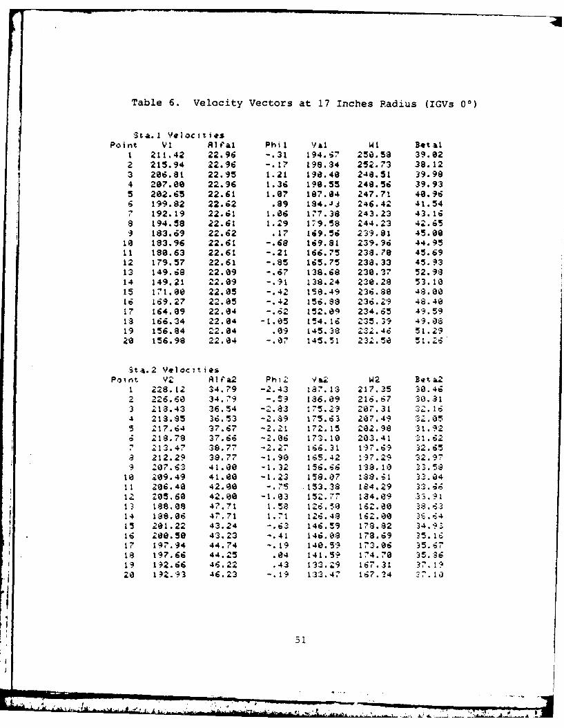
Table 6. Velocity Vectors at 17 Inches Radius (IGVs 00)
Sta.1 VeoCiiesPoint VI Rh'al Phil Val WL Bet.l
1 211.42 22.96 -.31 194.!i7 250.58 39.022 215.94 22.96 -. 17 198.34 252.73 38.123 206.81 22.95 1.21 190.40 248.51 39.984 207.00 22.96 1.36 190.55 248.56 39.935 202.65 22.61 1.07 187.04 247.71 40.966 199.82 22.62 .89 184.Ji 246.42 41.547 192.19 22.61 1.06 177.38 243.23 43.168 194.58 22.61 1.29 179.58 244.23 42.659 183.69 22.62 .17 169.56 239.81 45.00
10 183.96 22.61 -.68 169.81 239.96 44.9511 180.63 22.61 -.21 166.75 238.70 45.6912 179.57 22.61 -.85 165.75 238.33 45.9313 149.68 22.09 -.67 138.68 230.37 52.9314 149.21 22.09 -.91 138.24 230.28 53.1015 171.80 22.05 -.42 158.49 236.88 48.0016 169.27 22.05 -.42 156.98 236.29 48.4017 164.09 22.04 -.62 152.09 234.65 49.5918 166.34 22.04 -1.05 104.16 235.39 49.0619 156.84 22.04 .09 145.38 232.46 51.2920 156.98 22.04 -.07 145.51 232.50 51.2
Sta. 2 VelocitiesPo i nt & i1a2 Ph2 W2 Beta2
1 228.12 34.79 -2.43 187.1$ 217.35 30.462 226.60 34.79 -.19 186.09 216.67 30.313 218.43 36.54 -2.8a3 175.29 207.31 32.164 213.85 36.53 -2.89 175.6:3 207.49 :32.a55 Z17.64 37.67 -2.21 172.15 202.98 31.926 218.79 37.66 -2.6 173.10 203.41 31.627 213.47 38.77 -2.27 I .:31 197.69 32.65
a 212.29 38.77 -1.90 165.42 197.29 32.979 207.63 41.00 -1.32 1.6.66 133. I 33.58
18 209.49 41.00 -1.23 158.07 188..1 3.3.a411 206.40 42.8 -.75 .153.38 184.29 33.6612 295.60 42.90 -1.83 152.77 134.09 3:3.9113 188.08 47.71 1.58 126.50 162.00 38.6:314 188.06 47.71 1.71 126.48 162.-3.,415 201.22 43.24 -.63 146.59 178.82 34.9.316 200.50 43.23 -.41 146.08 179.69 3 5.1617 197.94 44.74 -. 19 140.59 173.06 35.6718 197.66 44.25 .04 141.59 174.70 35.361? 192.66 46.22 .43 133.29 167.31 37.1920 192.93 46.23 -. 19 1:33.4. 167.34 :37.18
51
i. . -V -
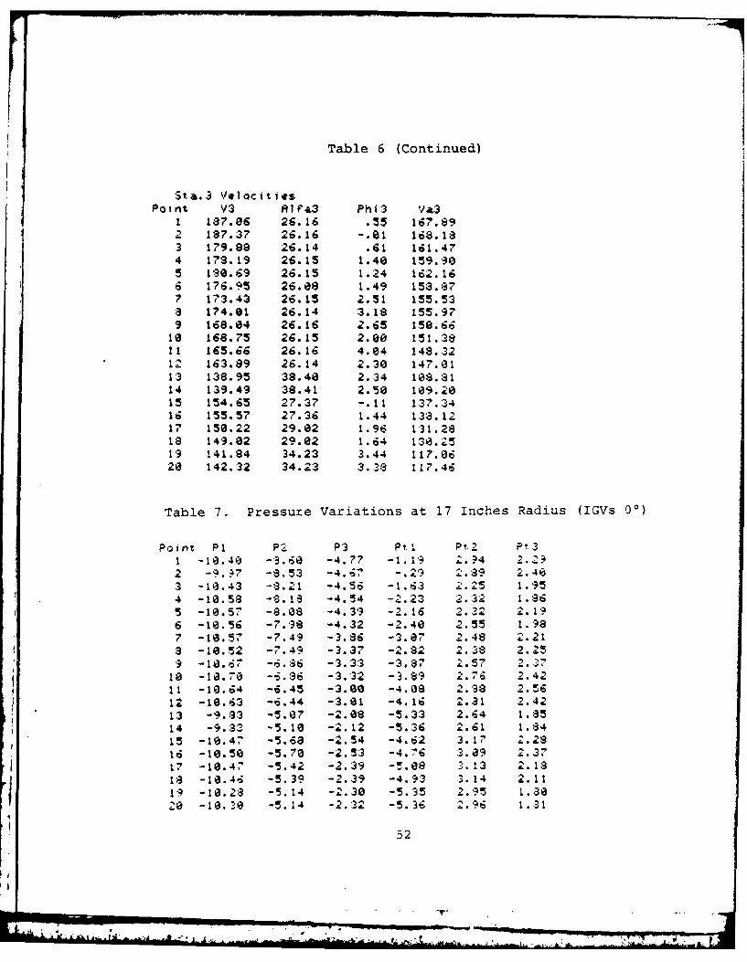
Table 6 (Continued)
Sta.3 VelocitiesPoint V3 A1pa3 Phi3 va3
1 187.66 26.16 .55 167.892 187.37 26.16 -.81 168.183 179.88 26.14 .61 161.474 173.19 26.15 1.40 159.905 190.69 26.15 1.24 162.166 176.95 26.68 1.49 15a.877 173.43 26.15 2.51 155.538 174.01 26.14 3.18 155.979 168.04 26.16 2.65 150.6610 168.75 26.15 2.00 151.38it 165.66 26.16 4.04 148.3212 163.89 26.14 2.30 147.0113 138.95 38.44 2.34 168.8114 139.49 38.41 2.50 109.2015 154.65 27.37 -.11 1:37.:S416 155.57 27.36 1.44 13a.1217 150.22 29.02 1.96 131.2918 149.02 29.02 1.64 136.2519 141.84 34.23 3.44 117.0620 142.32 34.23 3.'8 117.46
Table 7. Pressure Variations at 17 Inches Radius (IGVs 0*)
Point P1 P2 P:3 P1.l Pt2 Pt31 -16.40 -3.0 -4.77 -1.19 2.?4 2.232 -9. -8.53 -4.67 -.29 2.89 2.4;3 -16.43 2 1 -4.56 -1.63 2.25 1.954 -18.58 -8.18 -4.54 -2.23 2.32 1.865 -10.57 -8.08 -4.39 -2.16 2.22 2.196 -16.56 -738 -4.32 -2.40 2.55 1.987 -16.57 -7.49 -:3.86 -3.07 2.48 2.218 -10.52 -7.49 -3.37 -2.82 2.38 2.259 -1a.67 -6.86 -:3.3:3 -3.87 2.57 2. 7
10 -10.70 -6.36 -3.32 -3.8'9 2.76 2.4211 -10.64 -6.45 -3.00 -4.08 2.38 2.5612 -10.63 -6.44 -3.01 -4.16 2.81 2.4213 -9.83 -5.07 -2.68 -5.33 2.64 1.8514 -9.8,) -5.10 -2.12 -5.36 2.61 1.,415 -10.47 -5.68 -2.54 -4.62 3.17 2.2816 -10.50 -5.70 -2.53 -4.76 3.09 2.3717 -10.4' -5.42 -2.39 -3.0 .13 2.1818 -10.46 -5.39 -2.39 -4.93 3.14 2.11I' -10.28 -5.14 -2.30 -5.35 2. 95 1.'8.26 -10.38 -5.14 -2.32 -5.36 2.96 1.31
52
L ± .- I ., . .U .. ,.,, _L 'L .. . ... ... " .. ... ... " ... .. ,,- , ; .- . . 0. .. .. . [ 7 .T -
t
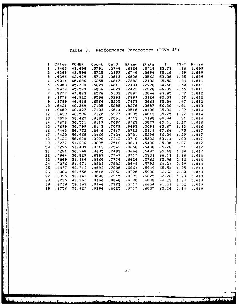
Table 8. Performance Parameters (IGVs 40)
I C'low POWER Cwork Cpt3 Etaav Etats T T3-T Prise1 .9405 43.608 .5701 .3948 .6926 .0718 63.73 .10 1.0092 .9389 43.598 .5725 .3859 .6740 .0694 65.10 .39 1.0093 .9396 43.929 .5743 .3813 .6638 .0562 63.30 1.35 1.0094 .9011 45.686 .6255 .4617 .73a2 .2133 65.52 -. 34 1.011
5 .9053 45.733 .6229 .4611 .7404 .2228 64.60 .50 1.0116 .9018 45.509 .6236 .4629 .742.32 63 -5 "l
7 .8777 47.003 .6576 .5133 .780"1 .3046 63.0- .7 1.0128 .3778 46.922 .6596 .520:3 .7889 .3124 65.59 .57 1.012
9 .8739 46.818 .6566 .5235 .7973 3063 65.04 .47 1.01210 .8421 48.369 .7105 .5880 .8276 .3887 66.36 -.01 1.01:311 .3409 48.427 .7103 .6044 .8510 .4106 65.32 .79 1.01412 .8423 48.586 .7120 .5977 .8395 .4013 65.75 1.27 1.01413 .7696 50.423 .8105 .7061 .8712 .5108 66.94 .91 1.01614 .7678 50.551 .8119 .7087 .8728 .5079 65.31 2.27 1.01615 .7699 50.799 .143 .7079 .3693 .5093 65.67 1.83 1.81616 .7443 50.752 3446 .7417 .37832 .5319 67.64 .75 1.01717 .7420 50.960 .3466 .7434 .371 .5290 66.09 1.29 1.01718 .7436 50.823 .8396 .7343 a746 .5333 63.14 .63 1.01719 .7277 51.336 .8695 .7516 .644 .5406 65.00 1-:37 1.01720 .7295 51.489 .8713 .7543 .8658 .5438 65.73 .51 I.81721 .7231 50.943 .8635 .7483 .3666 .5487 65.68 1.00 1.01722 .7064 50.329 .8389 .7749 .9717 .533 66.13 1.36 I. 1323 .7069 51.384 .A960 .77:30 .8626 .762 65.06 2. 33 1 .1324 .7076 51.071 .8883 .7682 .8648 .5793 64.24 2 .9 1.01325 .-87. 50.713 .9098 .7380 .3661 5949 65.54 i.5 1.O1'
26 .6334 50.550 .9010 71356 .3720 5996 62.66 2.68 1 .0127 .6a95 50.141 .9002 .7915 3793 .6025 37.2E :.29 1.01328 .675 49.967 .9166 .3048 817S0 .6083 66.23 1 .2 1.O1l29 .6720 50.163 .9146 .7972 .8717 .6034 61.:' 3.02 I01'?30 .6756 50.427 .9206 0S25 .3717 .60:37 65.36 :.34 19
53
w , - I---to 0
-L- I A I - - ,.

Table 9. Mid-span Velocity Vectors (IGVs 40).
Sta.1 VelocitiesPoint VI Rifal Phil Vai WI Bet lL
1 224.43 26.81 -3.16 289.46 243.48 30.504 219.94 20.80 -3.05 205.31 240.73 31.34
7 218.86 29.83 -2.94 196.82 23S.17 33.87
10 203.55 28.82 -2.97 190.80 230.98 34.54
13 188.44 -1147.45 -3.27 72.15 384.64 79.17
16 182.80 26.a2 -2.98 170.64 219.96 39.00
19 179.58 20.83 -3.13 167.59 218.23 39.73
22 174.71 28.81 -3.17 163.86 215.95 48.87
25 170.93 28.83 -3.22 159.42 214.09 41.77
28 167.07 28.83 -3.43 155.87 212.40 42.68
Sta.2 VelocitiesPoint V2 Alfa2 Phi2 Va2 W2 Beta2
1 243.93 33.31 -.26 203.95 215.27 18.75
4 236.37 34.44 -.49 194.93 206.95 19.62
7 233.13 35.27 -1.75 198.24 202.29 19.80
10 227.69 36.28 -1.16 183.51 195.89 20.45
13 219.03 38.38 -.87 171.68 184.37 21.36
r6 216.12 39.26 -1.0 167.31 180.02 21.64
19 213.83 39.98 -.66 163.83 176.54 21.S6
22 212.17 41.01 -1.12 160.07 172.48 21.77
'5 289.48 41.49 -.a2 156.90 169.60 22.28
.3 287.63 42.09 -.42 154.07 166.a2 22.54
Sta.3 VelocitiesPoint V3 A1t 3 Phi3 3
1 217.56 18.72 -3.08 205.75
4 210.45 18.71 2.2 1 .s187 206.52 13.46 -.75 1?5.88
10 200.62 18.47 1.41 190.'3
13 188.81 13.48 3.37 173.76
16 183.06 18.47 4.53 173.39
19 176.81 18.59 4.93 166.96
22 155.82 19.82 4.32 146.17
25 145.63 24.05 1.25 132.95
28 144.31 26.93 -1.7:3 128.60
54
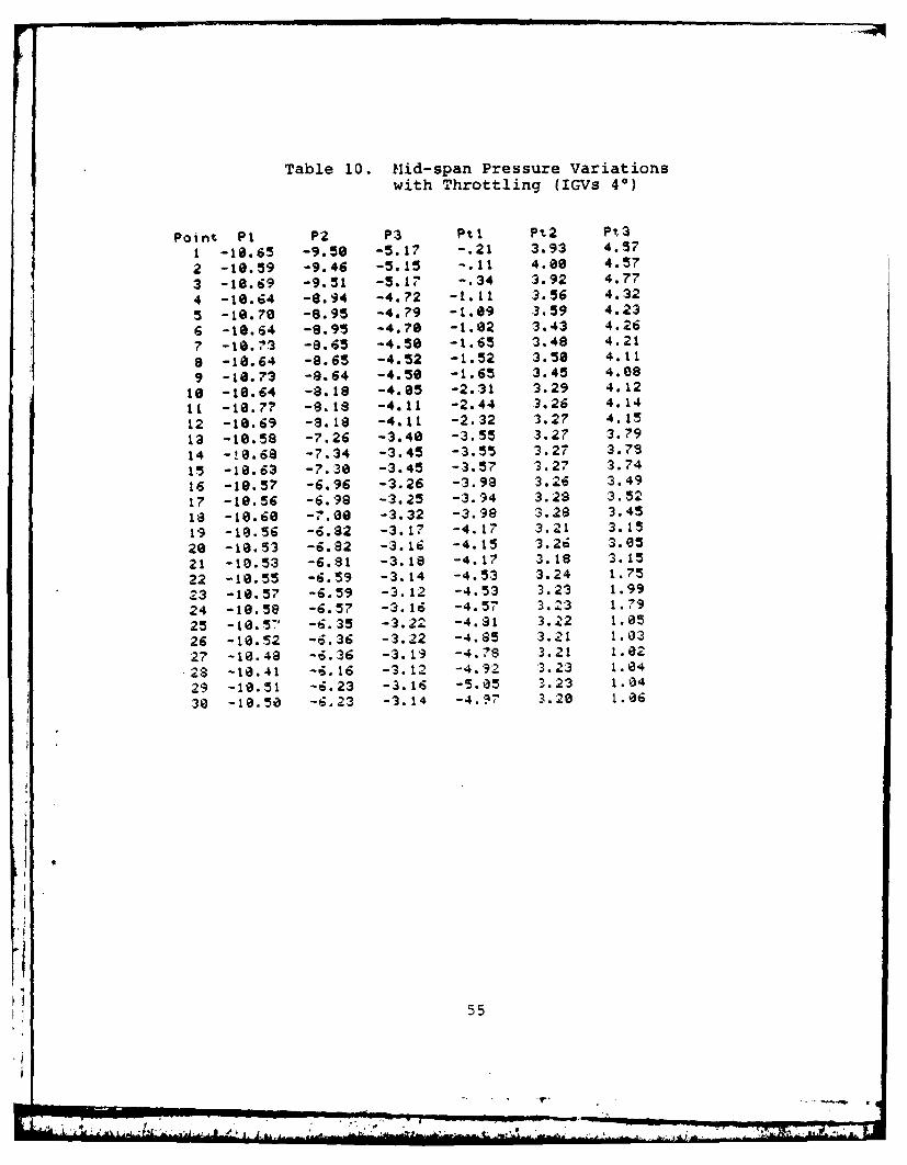
Table 10. Mid-span Pressure Variationswith Throttling (IGVs 40)
Point PI P2 P3 P%1 P%2 PO
1 -18.65 -9.50 -5.17 -.21 3.93 4.57
2 -10.59 -9.46 -5.15 -.11 4.00 4.57
3 -10.69 -9.51 -5.17 -.34 3.92 4.77
4 -18.64 -8.94 -4.72 -1.11 3.56 4.32
5 -10.76 -9.95 -4.79 -1.09 3.59 4.23
6 -16.64 -8.95 -4.76 -1.62 3.43 4.26
7 -18.73 -8.65 -4.56 -1.65 3.48 4.21
9 -10.64 -8.65 -4.52 -1.52 3.50 4.11
9 -16.73 -8.64 -4.50 -1.65 3.45 4.08
16 -16.64 -8.19 -4.65 -2.31 3.29 4.12
it -16.77 -8.18 -4.11 -2.44 :3.26 4.14
12 -18.69 -8.18 -4.11 -2.32 3.27 4.15
1a -10.58 -7.26 -3.46 -3.55 3.27 3.79
14 -!0.68 -7.34 -3.45 -3.55 3.27 3.78
15 -18.63 -7.38 -3.45 -:3.57 3.27 3.74
16 -1e.57 -6.96 -3.26 -3.98 :3.26 3.49
17 -10.56 -6.98 -3.25 -3.94 3.28 3.52
18 -18.68 -7.00 -3.32 -3.98 3.28 3.45
19 -10.56 -6.82 -3.17 -4.17 3.21 3.15
26 -10.53 -6.82 -3.16 -4.15 3.26 3.05
21 -10.53 -6.81 -3.18 -4.17 3.18 3.15
22 -18.55 -6.59 -3.14 -4.53 3.24 1.75
23 -18.57 -6.59 -3.12 -4.53 :3.23 1.99
24 -16.58 -6.57 -3.16 -4.57 3.23 1.79
25 -10.57 -6.35 -3.22 -4.81 3.22 1.05
26 -10.52 -6.36 -3.22 -4.85 3.21 1.0327 -10.48 -6.36 -3.19 -4.78 3.21 1.0228 -10.41 -6.16 -3.12 -4.92 :3.23 1.0429 -10.51 -6.23 -3.16 -5.05 3.23 1.84
30 -10.5S -6.23 -3.14 -4.97 3.20 1.06
55
A At ,AL'. t . ,L7
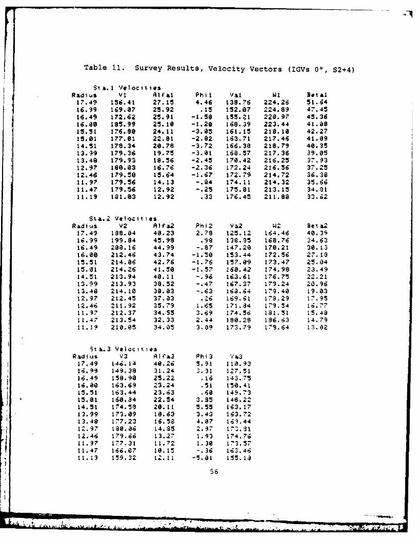
Table 11. Survey Results, Velocity Vectors (IGVs 0*, S2+4)
StA.1 VulocitiesRadius VI R1fal Phil Val W1 Detal17.49 156.41 27.15 4.46 138.76 224.26 51.6416.99 169.07 25.92 .15 152.07 224.89 47.4516.49 172.62 25.91 -1.58 155.21 220.97 45.3616.00 185.99 25.10 -1.20 168.39 223.44 41.0815.51 176.80 24.11 -3.05 161.15 218.10 42.2715.01 177.81 22.81 -2.82 163.71 217.46 41.0914.51 178.34 28.78 -3.72 166.38 218.79 40.3513.99 179.36 19.75 -3.01 168.57 217.36 39.0513.48 179.93 18.56 -2.45 178.42 216.25 37.9312.97 180.03 16.76 -2.36 172.24 216.56 37.2512.46 179.58 15.64 -1.67 172.79 214.72 36.3811.97 179.56 14.13 -.84 174.11 214.32 35.6611.47 179.56 12.92 -.25 175.01 213.15 34.8111.19 181.83 12.92 .33 176.45 211.88 :33.62
Sta. 2 Velocities
Radius V2 A1fa2 Phi2 Va2 Beta217.49 188.04 48.23 2.78 125.12 164.46 40.3916.99 199.84 45.98 .98 1:38.95 168.76 34.6316.49 208.16 44.99 -.87 147.28 170.21 30.1:316.88 212.46 43.74 -1.50 153.44 172.56 27.1815.51 214.86 42.76 -1.76 157.09 173.47 25.8415.01 214.26 41.50 -1.57 160.42 174.98 23.4914.51 213.94 48.11 -.96 163.61 176.75 22.2113.99 213.93 38.52 -.47 167.37 179.24 20.9613.48 214.10 38.03 -.63 168.64 179.40 19.0:312.97 212.45 37.,33 .126 169.61 17a.29 17.9512.46 211.92 35.79 1.65 171.84 179.54 16.7711.97 212.37 34.55 3.69 174.56 181.51 15.4811.47 213.54 32.33 2.44 180.29 186.63 14.7911.19 210.05 34.05 3.09 173.79 179.64 13.02
Sta.3 VelocitiesRadius V3 Rlfa3 Phi3 'a317.49 146.14 40.26 5.91 110.9316.99 149.38 31.24 ;.31 127.5116.49 158.90 25.22 .16 143.7516.00 163.69 23.24 .51 150.4115.51 163.44 23.63 .60 149.7315.01 168.84 22.54 3.85 148.2214.51 174.58 20.11 5.55 163.1713.99 173.09 18.63 3.43 163.7213.48 177.23 16.58 4.07 1639.4412.97 180.06 14.85 2.97 17".'3112.46 179.66 13.27 1.93 174.7611.97 177.31 11.72 1.30 173.5711.47 166.07 10.15 -..36 163.4611.19 159.32 12.11 -5.01 155.1.3
56
4*4 .,..K

Table 12. Performance Parameters (IGVs 30)
I Ct1ow POWER Cwork Cpt3 Etaav Etats T T3-T Prise1 .9520 45.132 .5842 .3923 .6715 .0551 64.81 .36 1.80892 .9518 44.889 .5844 .3969 .6791 .8623 66.99 -.75 1.0893 .9109 47.409 .6427 .4788 .7451 .2035 65.13 .91 1.0114 .9116 47.184 .6408 .4717 .7362 .1948 66.41 .15 1.8115 .8872 48.568 .6773 .5443 .8036 .3115 66.12 .85 1.8126 .8872 48.318 .6721 .52?0 .7970 .2968 64.96 -.70 1.8127 .a460 49.860 .7295 .610 .8361 .3970 66.17 1.17 1.0148 3496 49.236 .7247 .6944 .8340 .3897 65.41 1.16 1.6149 .7733 51.773 .8261 .7166 .8602 .5049 64.72 2.45 1.01610 .7754 51.110 .8165 .7117 .9717 .5120 66.73 2.37 1.01611 .7197 51.743 .8913 .7583 .3508 .5168 67.19 1.36 1.01712 .7528 52.366 .8551 .7515 .8789 .5362 63.34 2.65 1.01713 .7230 51.892 .89870 .7768 .8691 .5456 65.55 :3.16 1.01814 .7316 51.859 .8787 .7740 .8809 .5534 67.14 2.21 I.1:315 .7045 51.614 .9028 .7827 .8677 .5757 63.57 1.91 1.01316 .7145 51.586 .8930 .7870 .8813 .5863 65.96 •97 1.31817 .7048 52.307 .9144 .7321 .8553 .5636 63.92 1.77 1.01118 .711? 52.49 .9639 .7795 .8623 .5767 62.13 2.50 1.81819 .6374 51.733 .9259 .7931 .8565 .5924 63.21 2.45 1.81:,20 .6898 51.750 .9287 .7886 .8565 .5926 61.94 1.87 1.01S21 .6785 51.880 .9291 .9041 .8655 .6866 64.34 1.65 1.1?22 .6810 50,907 .9239 .3044 .8786 .6892 65.60 1.68 1.019
II i
57
L A_-

Table 13. Mid-span Velocity Vectors (IGVs 30)
Sta.1 VelocitiesPoint Vi Alal Phil Val WI Betal
1 226.28 20.08 -3.07 212.22 246.84 30.573 218.47 20.24 -2.98 204.78 241.56 31.925 212.22 20.6? -3.00 199.06 238.23 33.207 264.54 26.6? -2.81 191.89 233.69 34.789 189.16 28.68 -2.62 177.42 225.16 37.91
11 182.83 28.89 -2.83 171.56 221.92 39.2813 179.35 28.67 -2.43 168.31 228.11 40.0615 174.79 26.67 -2.91 163.97 217.91 41.1117 175.69 26.68 -2.97 164.86 218.31 46.9619 178.52 28.89 -2.89 159.94 215.83 42.1621 168.23 20.06 -3.09 157.79 214.89 42.66
Sta.2 Ye)ocititePoint V2 Rlf'a2 Phi2 VI2 W2 BetaZ
1 246.56 33.29 -.71 206.04 216.92 18.213 239.52 34.28 -1.82 197.82 269.35 19.025 234.48 35.02 -.82 192.01 203.89 19.647 230.62 36.01 -.;34 186.05 198.86 20.049 219.60 38.37 -.89 1'72.15 1.34.67 21.29
11 216.25 39.12 -1.82 167.74 136.52 21.6613 214.24 39.50 -1.04 165.28 179.30 22.0115 211.37 46.24 -.88 161.33 174.53 22.4217 211.95 40.23 -1.17 161.78 174.83 22.2519 269.09 41.23 -.99 157.22 170.26 22.5521 207.42 41.61 -.67 155.07 168.30 22.36
St.&.3 VelocitiesPoint %J3 R1fa3 Phi3 Ya3
1 221.95 18.25 -3.11 210.473 239.73 28.30 -2.71 196.495 205.16 20.30 -2.47 192.237 197.44 28.38 -1.82 185.089 186.1.3 20.67 -.82 174.13
11 182.82 21.34 -1.23 170.2513 181.27 22.12 .82 167.9115 179.51 22.13 2.47 166.1317 179.60 23.23 1.98 164.9519 177.87 24.31 2.75 161.9121 176.90 24.96 3.19 160.13
58
"---------------------- ---

Table 14. Mid-span Pressure Variationswith Throtting (IGVs 30)
Point P1 P2 P3 Ptl Pt& P%31 -10.85 -9.63 -5.34 -.23 4.08 4.832 -10.91 -9.57 -5.27 -.65 4.17 4.743 -10.76 -9.08 -4.92 -.97 3.73 4.024 -10.85 -9.11 -4.98 -1.35 3.79 4.893 -1.73 -8.73 -4.78 -1.58 3.51 3.816 -10.80 -8.81 -4.74 -1.66 3.50 3.727 -10.78 -8.32 -4.27 -2.35 3.40 3.578 -10.82 -8.35 -4.32 -2.37 3.34 3.509 -10.73 -7.35 -3.43 -3.60 3.26 3.511 -10.69 -7.35 -3.43 -3.60 3.24 3.5311 -10.65 -6.98 -3.17 -4.05 3.24 3.5012 -10.65 -7.81 -3.19 -4.01 3.32 3.5413 -10.64 -6.78 -3.05 -4.26 3.23 3.5314 -19.65 -6.79 -3.07 -4.24 3.21 3.5015 -109.69 -6.63 -3.03 -4.63 3.17 3.4816 -10.65 -6.58 -2.99 -4.60 3.17 3.4717 -10.74 -6.67 -3.83 -4.62 3.17 3.4813 -10.75 -6.68 -3.83 -4.59 3.20 3.4919 -10.63 -6.41 -2.95 -4.86 3.15 3.4420 -18.9 -6.43 -2.96 -4.91 3.16 3.4321 -10.61 -6.25 -2.92 -5.02 3.14 3.3922 -18.60 -6.25 -2.92 -5.05 3.13 3.38
59
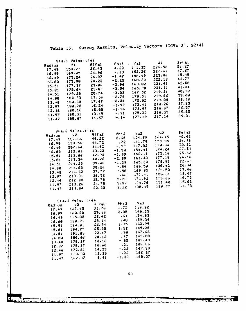
Table 15. Survey Results, Velocity Vectors (IGVs 30, S2+4)
Sta.1 VelocitiesRadius VI RIfa Phil Val WI Betal
17.49 158.21 26.43 4.20 141.35 226.53 51.27
16.99 169.05 24.96 -.19 153.26 227.61 47.6?
16.49 173.24 24.9? -1.47 156.99 223.86 45.45
16.08 175.90 24.22 -2.25 168.30 222.13 43.77
15.51 177.37 23.02 -2.96 163.82 221.41 42.50
15.81 178.64 21.6? -3.54 165.70 221.11 41.34
14.51 179.38 20.74 -3.03 167.52 219.31 40.10
14.00 180.73 19.16 -2.78 178.51 219.66 39.08
13.48 188.68 17.67 -2.34 172.82 219.00 38.18
12.97 180.72 16.24 -1.97 173.41 218.26 37.35
12.46 180.16 15.00 -1.36 173.97 216.67 36.57
11.97 180.31 13.49 -.91 175.32 216.33 35.85
11.47 188.8" 11.57 -.14 177.19 217.14 35.31
Sta.2 VelocitiesRadius V2 Alf&2 Phi2 Va2 W2 Bet a2
17.49 117.36 48.22 2.65 124.69 164.45 40.62
16.99 199.56 44.72 . 2 141.79 173.05 -4.98
16.49 207.64 44.92 -.97 147.02 170.34 30.32
16.00 212.01 43.22 -1.98 154.41 174.24 27.54
15.51 213.66 42.23 -1.99 158.11 175.16 25.42
15.01 213.34 48.76 -2.89 161.48 177.19 24.16
14.51 214.23 39.4a -1.29 165.38 178.93 22.47
14.80 214.68 38.26 -.59 168.50 18.42 20.94
13.4a 214.62 37.77 -.56 169.65 179.50 19.16
12.97 213.31 36.52 .68 171.41 180.31 13.47
12.406 212.88 35.78 2.23 171.92 179.66 16.13
11.97 213.26 34.78 3.87 174.76 131.40 15.0s
11.47 213.64 32.30 2.22 180.45 i96.77 14.7S
Sta.3 Velocitie;Radius V3 PIfa3 Phi3 V-a3
17.49 137.45 31.76 1.72 116.82
16.99 160.A0 29.16 2.35 140.25
16.49 175.82 28.42 .61 154.63
16.08 130.71 28.14 .48 159.34
15.51 184.01 26.94 1.35 163.99
15.81 184.77 25.85 1.22 149.28
14.51 181.03 22.17 .90 167.63
14.80 186.86 28.13 .47 169.80
13.48 178.37 1a.16 -.85 169.48
12.97 175.37 16.60 .21 168.;6
12.46 172.81 14.39 -.23 167.39
11.97 170.33 12.38 -.23 166.37
11.47 162.37 8.91 -1.33 160.37
60
II1 'L -.. . ' t - i L
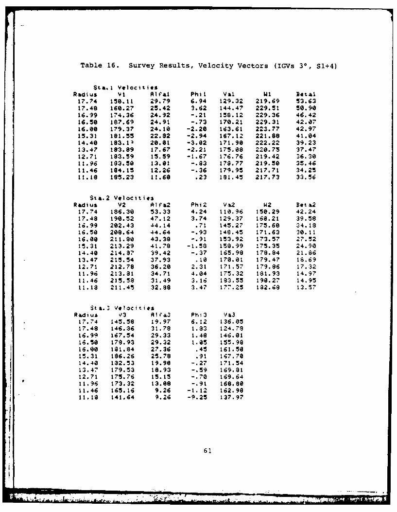
Table 16. Survey Results, Velocity Vectors (IGVs 30, S1+4)
Sta.1 VelocitiesRadius Vl Alfal Phil Val Wi Betal17.74 150.11 29.79 6.94 129.32 219.69 53.6317.48 168.27 25.42 3.62 144.47 229.51 50.9016.99 174.36 24.92 -.21 158.12 229.36 46.4216.50 187.69 24.91 -.73 170.21 229.31 42.3716.0 179.37 24.10 -2.20 163.61 223.77 42.9715.31 181.55 22.92 -2.94 167.12 221.88 41.0414.40 183.11 20.01 -3.02 171.90 222.22 39.2313.47 183.89 17.67 -2.21 175.08 220.75 37.4712.71 183.59 15.59 -1.67 176.76 219.42 36.3011.96 183.50 13.01 -.83 178.77 219.50 35.4611.46 184.15 12.26 -.36 179.95 217.71 34.2511.18 185.23 11.68 .23 181.45 217.73 33.56
Sta.2 VelocitiesRadius Y2 Rlfa2 Phi2 Va2 W2 Beta217.74 186.30 53.33 4.24 110.96 150.29 42.2417.48 190.52 47.12 3.74 129.37 168.21 39.5816.99 202.43 44.14 .71 145.27 175.60 34.1816.50 208.64 44.64 -.93 148.45 171.63 30.1116.00 211.88 43.38 -.91 153.92 173.57 27.5215.31 213.29 41.78 -1.58 158.99 175.35 24.9014.40 214.87 39.42 -. 37 165.98 178.84 21.8613.47 215.54 37.93 .10 170.01 179.47 18.6912.71 212.78 36.20 2.31 171.57 179.86 17.3211.96 213.81 34.71 4.04 175.32 181.93 14.9711.46 215.58 31.49 3.16 183.55 190.27 14.9511. 18 211.45 32.88 3.47 177.25 12.68 13.57
Sta. 3 Velocities
Radius V3 Rla3 Phi3 Va317.74 145.58 19.97 6.12 136.0517.48 146.36 31.78 1.3 124.7916.99 167.54 29.33 1.48 146.0116.50 179.93 29.32 1.05 155.9816.80 181.84 27.36 .45 161.5015.31 186.26 25.78 .91 167.7014.40 132.53 19.98 -. 27 171.5413.47 179.53 18.93 -.59 169.8112.71 175.76 15.15 -. 70 169.6411.96 173.32 13.88 -.91 168.8011.46 165.16 9.26 -1.12 162.9811.18 141.64 9.26 -9.25 137.97
61
&A . .1I
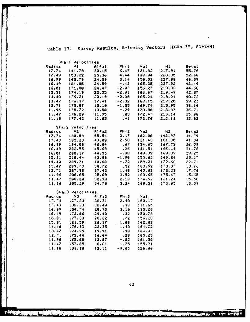
Table 17. Survey Results, Velocity Vectors (IGVs 3, Sl+2+4)
Sta. 1 VelocitiesRadius V1 RIfal Phil V-1 WI Betal17.74 141.78 30.15 6.47 121.32 217.91 55.7617.49 153.22 25.36 4.44 138.64 228.35 52.6816.99 165.79 24.59 3.14 150.52 227.88 48.5916.49 181.85 24.59 -. 43 165.35 227.92 43.4916.61 171.80 24.47 -2.87 156.27 219.93 44.6815.31 174.19 22.55 -2.91 160.67 219.49 42.8714.40 176.21 28.19 -2.38 165.24 218.24 40.7313.47 176.37 17.41 -2.32 163.15 217.28 39.2112.71 175.87 15.18 -1.55 169.74 215.95 38.1611.96 175.72 13.58 -. 29 170.80 213.07 36.7111.47 176.29 11.95 .03 172.47 213.14 35.9311.18 177.42 11.65 .41 173.76 212.18 35.82
Sta.2 VelocitiesRadius V2 Rlfa2 Phi2 V&2 W2 Bet&217.74 180.58 55.54 2.47 102.08 143.97 44.7917.49 185.28 49.00 2.58 121.43 161.98 41.3416.99 194.00 46.04 .67 134.65 167.73 36.5916.49 202.55 45.68 .26 141.51 166.44 31.7616.81 208.17 44.55 -.90 148.32 168.39 28.2515.31 210.44 43.08 -1.90 153.62 169.84 25.1714.40 299.71 40.60 -.72 159.21 172.60 22.7113.47 209.73 38.72 .52 163.62 173.37 19.7612.71 287.88 37.43 1.40 165.03 173.33 17.7611.96 208.05 35.69 3.52 163.65 175.47 15.6511.47 208.20 32.98 2.18 174.52 181.24 15.5611.18 205.29 34.70 3.24 168.51 173.65 13.59
St.&.3 VelocitiesRadius V3 lf&3 Phi3 Va317.74 127.83 38.31 2.98 10.1717.49 132.23 32.40 .38 111.6516.99 154.74 28.95 3.10 135.2816.49 173.66 29.43 .32 158.7316.01 177.38 28.22 .72 156.2815.31 181.59 26.37 1.60 162.6314.40 178.93 23.35 1.43 164.2213.47 174.95 19.91 .90 164.4712.71 172.46 16.64 .28 165.2311.96 165.68 12.87 -.82 161.50
11.47 157.05 8.61 -1.75 155.2111.18 131.38 12.11 -9.85 126.86
62
.1 . . ... .....
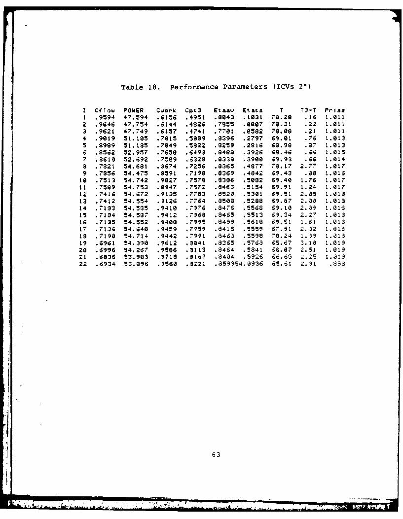
Table 18. Performance Parameters (IC-Vs 20)
I Cflow POWER Cwork Cpt3 Etaav Etats T T3-T Prize1 .9594 47.594 .6156 .4951 .8043 .1031 70.28 .16 1.0112 .9646 47.754 .6144 .4826 .7855 .0887 70.31 .22 1.0113 .9621 47.749 .6157 .4741 .7701 .0582 70.08 .21 1.0114 .9019 51.105 .7015 .5889 .8396 .2797 69.01 .76 1.0135 .8989 51.185 .7049 .5822 .8259 .2816 68.98 87 1.0136 .8562 52.957 .7650 .6493 .8488 .3926 68.46 .6S 1.0157 .3618 52.692 .7589 .6328 .8338 .3900 69.93 .66 1.014a .7821 54.681 .3674 .7256 .8365 .4877 70.17 2.77 1.0179 .7856 54.475 .8591 .7190 .8369 .4842 69.43 .00 1.01610 .7513 54.742 .9027 .7570 .8386 .5082 69.40 1.76 1.01711 .7589 54.753 .8947 .7572 .8463 .5154 69.91 1.24 1.01712 .7416 54.672 .9135 .7783 .8520 .5301 69.51 2.05 1.01813 .7412 54.554 .3126 .7764 .8508 .5288 69.87 2.00 1.01814 .7183 54.585 .9410 .7976 .8476 .5568 69.10 2.09 1.01S15 .7134 54.587 .9412 .7968 .8465 .5513 69.34 2.27 1.01816 .7185 54.552 .9408 .7995 .8499 .5618 69.51 1.61 1.01317 .7136 54.640 .9459 .7959 .0415 .5559 67.91 2.32 1.0LS18 .7190 54.714 .9442 .7991 .8463 .5598 70.24 1.39 1.01819 .6961 54.390 .9612 .8041 .3365 .5763 65.67 3.10 1.019?20 .6996 54.26? .9586 .311:3 .8464 .5841 68.07 2.51 1.01921 .6836 53.903 .9718 .8167 .8404 .5926 66.65 2.25 1.01922 .6934 53.896 .9560 .8221 .a59954.0936 65.61 2.31 .39a
63

Table 19. Mid-span Velocity Vectors (IGVs 20)
Sta.1 VelocitiesPoint VI ARfal Phil Val WI Betal
3 227.26 19.31 -2.94 214.19 249.83 30.865 213.72 19.54 -1.25 201.36 240.63 33.177 205.37 19.54 -2.20 193.40 235.70 34.809 190.04 19.54 -2.56 178.91 227.12 37.95
11 183.25 19.55 -2.58 172.51 223.53 39.4213 180.79 19.54 -2.78 170.18 222.31 39.9715 175.51 19.54 -3.20 165.15 219.73 41.1717 174.19 19.53 -2.89 163.95 219.07 41.4719 170.28 19.54 -3.13 160.24 217.21 42.3721 167.78 19.54 -3.24 157.86 826.58 78.97
Sta.2 VelocitiesPoint V2 Rlfa2 Phi2 V&2 W2 Bot.2
3 251.68 32.66 -1.39 211.81 222.31 17.625 238.27 -363.52 -2.81 237.54 322.63 42.517 230.73 35.63 -2.75 137.32 199.76 20.14• 220.55 37.84 -2.46 174.01 136.93 21.29
11 217.52 -83.30 -2.26 25.34 420.23 36.5413 215.67 39.87 -2.19 167.33 180.45 21.3315 212.35 40.08 -2.39 162.33 175.54 22.2417 211.48 40.08 -2.62 161.64 175.14 22.5019 209.07 40.32 -2.62 158.05 171.63 22.8021 201.41 42.80 -2.58 147.63 744.77 713.56
Sta.3 VelocitiesPoint V3 AI a3 Phi3 VaL3
3 221.70 19.34 -1.97 209.065 208.a5 119.74 -1.74 195.747 199.a4 288.23 -2.12 62.479 186.93 20.63 -1.21 174.93
11 184.06 21.37 -.48 171.4013 182.81 21.37 -. 07 170.2415 179.95 22.66 1.23 166.0317 179.60 22.82 .77 165.5319 178.15 23.94 2.20 162.7021 176.77 24.63 2.73 160.58
64
• ,I~~~~~~~~~~........ ..,................ .... '.....I ' " = ... ... .. '
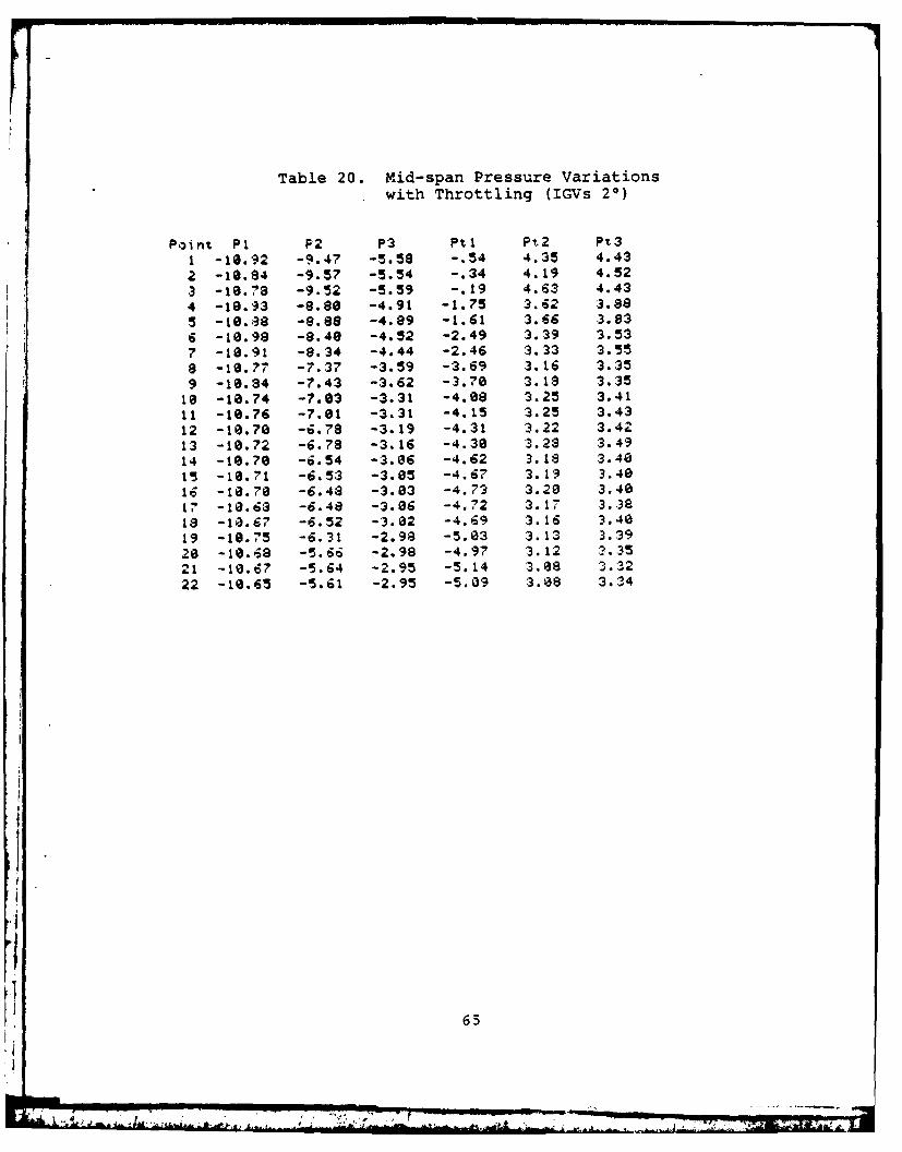
Table 20. Mid-span Pressure Variationswith Throttling (IGVs 20)
Point PI F2 P3 PtI Pt2 Pt31 -10.92 -9.47 -5.58 -.54 4.35 4.432 -10.84 -9.57 -5.54 -.34 4.19 4.523 -10.' -9.52 -5.59 -.19 4.63 4.434 -10.93 -8.80 -4.91 -1.75 3.62 3.885 -10.38 -8.88 -4.89 -1.61 3.66 3.836 -10.98 -8.40 -4.52 -2.49 3.39 3.537 -10.91 -8.34 -4.44 -2.46 3.33 3.558 -10.77 -7.37 -3.59 -3.69 3.16 3.359 -10.84 -7.43 -3.62 -3.70 3.18 3.3510 -10.74 -7.03 -3.31 -4.08 3.25 3.4111 -10.76 -7.01 -3.31 -4.15 3.25 3.43
12 -10.70 -6.78 -3.19 -4.31 3.22 3.4213 -10.72 -6.78 -3.16 -4.30 3.28 3.4914 -10.70 -6.54 -3.06 -4.62 3.18 3.4815 -10.71 -6.53 -3.05 -4.67 3.19 3.4016 -10.70 -6.48 -3.03 -4.73 3.20 3.401? -10.6a -6.48 -3.06 -4.72 3.17 3.3818 -1a.67 -6.52 -3.02 -4.69 3.16 3.4e19 -10.75 -6.31 -2.98 -5.03 3.13 :3.3920 -10.68 -5.66 -2.98 -4.97 3.12 :.3521 -10.67 -5.64 -2.95 -5.14 3.08 3.3222 -10.65 -5.61 -2.95 -5.09 :3.88 3.34
63
,
|."
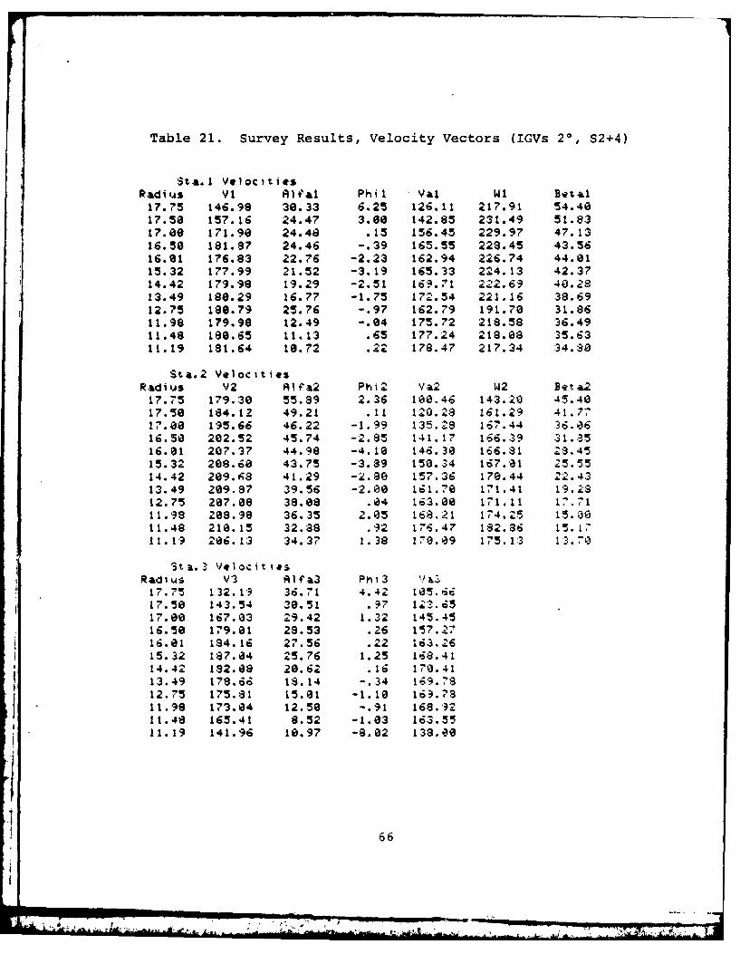
Table 21. Survey Results, Velocity Vectors (IGVs 20, S2+4)
Sta.1 VelocitiesRadius Vt Alfal Phil Val WI Betal17.75 146.98 30.33 6.25 126.11 217.91 54.4017.50 157.16 24.47 3.68 142.85 231.49 51.8317.00 171.90 24.48 .15 156.45 229.97 47.1316.50 181.87 24.46 -.39 165.55 228.45 43.5616.01 176.83 22.76 -2.23 162.94 226.74 44.0115.32 177.99 21.52 -3.19 165.33 224.13 42.3714.42 179.98 19.29 -2.51 169.71 222.69 40.2813.49 180.29 16.77 -1.75 172.54 221.16 38.6912.75 188.79 25.76 -.97 162.79 191.78 31.8611.98 179.98 12.49 -.04 175.72 218.58 36.4911.48 180.65 11.13 .65 177.24 218.08 :35.6311.19 181.64 16.72 .22 178.47 217.34 34.80
Sta.2 VelocitiesRadius V2 Alfa2 Phi2 Va2 W2 Beta217.75 179.30 55.89 2.36 106.46 143.20 45.4017.50 184.12 49.21 .11 120.28 161.29 41.7717.00 195.66 46.22 -1.99 135.29 167.44 36.0616.50 202.52 45.74 -2.85 141.17 166.39 31.9516.01 207.37 44.98 -4.10 146.38 166.81 29.4515.32 208.60 43.75 -3.89 156.34 167.01 25.5514.42 209.08 41.29 -2.80 157.36 170.44 22.4313.49 209.87 39.56 -2.80 161.70 171.41 19.2312.75 207.08 38.68 .04 163.60 171.11 17.7111.98 208.98 36.35 2.05 168.21 174.25 15.0011.48 210.15 32.88 .92 176.47 182.86 15.1711.19 206.13 34.3? 1.38 170.09 175.13 1:3.70
StA.3 Velocities
Radius V3 Alfa2 Ph1317.75 132.19 36.71 4.42 105.6617.50 143.54 30.51 .97 123.6517.80 167.03 29.42 1.32 145.4516.50 179.61 28.53 .26 157.2716.01 184.16 27.56 .22 163.2615.32 187.04 25.76 1.25 168.4114.42 182.08 20.62 .16 170.4113.49 178.66 18.14 -. 34 169.7812.75 175.81 15.01 -1.10 16?.7811.98 173.04 12.50 -.91 168.9211.48 165.41 8.52 -1.03 163.5511.19 141.96 10.97 -8.62 138.00
66
n- At .1 31t I

Table 22. Survey Results, Velocity Vectors (IGVs 20, Sl+4)
sta.1 VelocitiesRadius Vt Rlf41 Phi I Val WI Betal17.75 149.93 28.18 5.69 131.51 223.65 53.7817.50 161.00 24.51 4.29 146.09 232.50 50.9417.01 171.04 24.42 .11 155.74 229.90 47.36
16.51 185.64 24.40 -. 27 169.05 230.12 42.72
16.02 179.34 22.77 -1.94 165.27 227.75 43.44
15.33 181.36 21.67 -2.43 168.39 225.20 41.55
14.42 182.96 19.34 -1.60 172.57 224.08 39.61
13.50 183.29 16.79 -1.67 175.40 222.92 38.08
12.74 183.26 14.47 -.42 177.44 222.26 37.03
12.74 183.18 14.46 -.94 177.35 222.24 37.05
11.99 182.25 12.25 -. 11 178.10 220.76 36.22
11.50 182.65 10.98 .55 179.30 219.93 35.38
11.21 134.01 10.85 1.08 180.68 218.36 34.314
Sta.2 Velocitiesadi V2 tI1fI2 Phi2 Va2 w B ta2
17.75 181.20 54.93 3.89 103.33 145.95 44.49
17.50 186.66 48.46 .95 123.77 163.78 48.87
17.01 197.09 46.22 -2.33 136.26 167.70 35.59
16.51 204.25 45.72 -2.88 142.43 166.90 .1.38
16.02 207.19 44.97 -3.27 146.34 166.81 28.5115.33 209.24 43.22 -3.89 152.13 !69.09 25.61
14.42 211.15 41.37 -2.98 158.24 170.87 41.9713.50 210.98 :39.24 -2.11 163.30 173.05 19.22
12.74 208.29 37.76 .16 164.67 172.71 17.55
12.74 203.88 37.77 .21 165.11 173.02 17.39
11.99 210.13 34.62 2.21 172.88 179.94 16.05
11.50 211.96 32.54 1.56 17. 62 185.06 15.0811.21 209.10 3:3.79 1.23 172.91 17S.06 13.76
sts.3 VelocitiesRadius 3 A I &3 Phi3 V 3
17.7t 138.55 35.60 3.73 112.4217.50 150.66 30.21 1.00 130.1817.01 169.78 29.26 1.21 148.0816.51 181.57 29.27 .53 159.9016.32 185.54 27.68 .58 164.2915.33 188.58 26.48 .65 168.7914.42 184.03 20.54 -. 39 172.3313.50 180.25 18.58 -1.04 170.8312.74 178.20 14.86 -1.05 172.2112.74 179.16 14.85 -1.32 172.1611.99 175.59 12.43 -. 76 171.4611.50 167.92 11.58 -1.22 164.4611.21 146.20 11.16 -7.69 142.15
67
-7-"
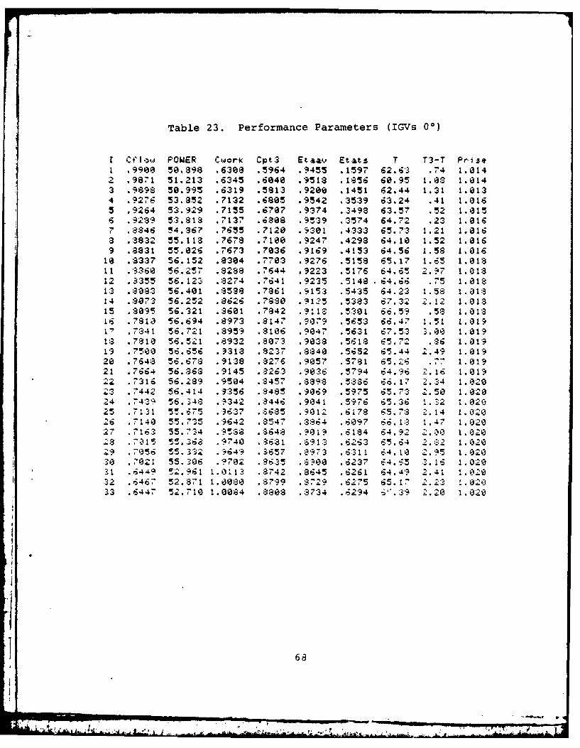
Table 23. Performance Parameters (IGVs 0)
I Cf1o,, POWER Cwork Cpt3 Etaav Etats T T3-T Prize1 .9900 50.398 .6308 .5964 .9455 .1597 62.6'3 .74 1.0142 .9871 51.213 .6345 .6040 .9518 .1856 60.95 1.8 1.0143 .9898 50.995 .6319 .5813 .9208 .1451 62.44 1.31 1.0134 .9276 53.852 .7132 .6805 .9542 .3539 63.24 .41 1.0165 .9264 53.929 .7155 .6707 .9374 .3498 63.57 .52 1.0156 9289 5:3.81a .7137 .6808 .9539 .3574 64.72 .23 1.0167 .846 54.967 .7655 .7120 .9301 .4333 65.73 1.21 1.0168 .3832 55.118 .7678 .7100 .9247 .4298 64.10 1.52 1.0169 .8831 55.026 .7673 .7036 .9169 .4153 64.56 1.58 1.01618 .8337 56.152 .8384 .7703 .9276 .5158 65.17 1.65 1.01811 .360 56. 257 .8288 .7644 .9223 .5176 64.65 2.97 1.01:312 .8355 56.123 .8274 .7641 .9235 .5148 . 64.66 .75 1.0181:3 .8083 56.401 .8538 .7861 .9153 .5435 64.23 1.58 I1.8114 .8073 56.252 .8626 .7880 .9125 .5383 67.32 2.12 1.01315 .8095 56.321 .3601 .7342 .911S .5301 66.59 .53 1.01316 .7813 56.694 .8973 .8147 .9079 .5653 66.47 1.51 1.01917 .7341 56.721 .8959 .8106 .9047 .5631 67.53 3.30 1.01918 .7810 56.521 .8932 .8073 .9033 .5613 65.7: .36 1.01919 .7500 56.656 .9313 a 3237 .8340 .5652 65.44 2.49 1.01920 .7643 56.673 .9138 .3276 .9057 .5781 65.26 .77 1.01921 .7664 56.363 .9145 .8263 .9036 5794 64.96 2.16 1.0192 .7316 56.289 .9504 .3497 .8898 .5336 66.17 2.34 1.02023 7442 56.414 9356 .8485 .9069 .5975 65. 73 2.50 1.020Z4 7433 56. 348 .9342 .8446 .9041 .5976 65.36 2 1.02025 71.31 55.675 .3637 .86-5 .9012 .6178 65.78 14 1.020'6 140 55.735 .9642 .8547 .3864 .6097 66.13 1.47 1.020
7 163 55.734 .9568 .3648 .9019 6184 64.92 2. 1.020
70 15 55. 36a 9740 .3631 .S913 .6263 65.64 1 . 0209 056 55.332 .'649 .:3657 ..:973 .6:311 4. 10 1.?5 1.020
:38 0 021 55.306 .702 .3635 .:300 .6237 4. 5 3.16 1.020I .6449 52.361 1 .0113 .3742 .8645 .6261 64. 49 2.41 1.k2032 .6467 52.871 1.0080 .3799 .8729 6275 65.17 2 1020:33 .6447 52.710 1.0034 .808 .3734 .6294 2-.39 1 .020
68

Table 24. Mid-span Velocity Vectors (IGVs 00)
Sta.1 VelocitiesPoint VI Rlfal Phil Val WI Btal
1 230.53 17.67 -4.25 219.05 257.06 31.304 213.17 17.26 -4.66 202.96 247.26 34.587 208.60 17.27 -4.52 198.58 244.43 35.42
10 198.53 17.25 -4.63 188.98 238.52 37.35
13 192.95 17.24 -4.76 183.64 235.39 38.4816 187.06 17.63 -4.56 177.72 231.01 39.4919 183.44 17.63 -4.40 174.31 229.05 40.2522 179.03 17.36 -4.34 170.38 227.46 41.3025 173.58 17.37 -4.08 165.25 224.62 42.4828 170.51 17.36 -4.12 162.33 223.12 43.1631 158.22 17.36 -4.70 156.51 217.41 46.61
Sta.2 VelocitiesPoint V2 Rlfa2 Phi2 Va2 W2 Bvta2
1 259.64 34.31 -1.14 214.42 221.,36 14.934 250.87 35.75 -1.07 202.92 210.82 15.707 241.22 :36.99 -1.20 192.63 281.22 16.76
10 231.32 .38.25 -1.46 181.60 191.29 13.2613 227.11 38.99 -1.59 176.46 186.54 18.8516 222.07 50.45 -1.65 141.35 144.96 12.7019 219.38 49.84 -1.84 141.42 145.87 14.8722 215.64 51.73 -1.67 133.51 137.78 14.2225 212.00 51.45 -1.93 1:32.05 137.30 15.7G28 210.19 51.45 -1.89 130.92 136.60 ;6,4831 205.37 51.86 -1.98 126.77 133.50 i.16
Sta.3 VelocitlesPoint V3 Alt'a3 Phi.3 Va3
1 226.92 23.19 -2.23 208.424 214.30 20.35 -2.95 200.657 204.76 20.35 -3.10 191.70
10 194.50 20.33 -3.40 182.0613 189.47 20.34 -2.70 177.4516 125.95 21.29 -1.67 173.0919 183.05 21.77 -1.61 169.93
- 181.44 22.31 -. 11 167.8625 179.45 23.12 .39 165.0428 178.30 23.44 .77 163.5731 174.86 24.36 1.21 159.26
69

Table 25. Survey Results, Velocity Vectors (IGVs 00, S1+4)
Sta.1 VelocitiesRadius VI Rlal Phil Val WI Betal17.98 143.47 35.43 11.85 114.41 209.29 56.0417.80 156.42 28.15 8.17 131.28 225.57 53.9917.65 157.55 24.23 6.49 142.75 235.01 52.3117.49 163.74 22.67 1.98 151.00 238.33 56.6617.25 172.79 23.01 .45 159.04 237.47 47.9517.00 176.44 21.86 -1.39 163.70 239.42 46.8516.75 179.10 22.37 -2.56 165.45 236.48 45.5416.50 190.65 22.20 -2.92 167.04 235.12 44.6516.50 180.85 22.20 -2.97 167.22 235.22 44.6116.81 184.12 21.84 -3.58 171.51 235.19 43.06
15.32 185.01 19.78 -4.78 173.48 232.78 41.5914.41 186.34 17.07 -4.46 177.59 232.55 40.0113.49 187.30 14.71 -3.76 189.77 231.05 38.3612.72 186.82 12.66 -3.11 182.01 229.30 37.35
11.98 186.80 10.72 -2.17 193.40 227.64 36.2711.48 186.48 9.18 -1.83 183.99 226.88 35.7711.19 189.57 8.59 -1.11 187.41 228.09 34.73
Sta.2 VelocitiesRadius V2 A1fa2 Phi2 'l/2 W2 Beta217.90 184.33 57.83 6.56 99.65 141.01 44.6617.80 184.03 54.42 3.09 1'6.92 148.00 43.6617.65 186.23 49.69 .75 120.47 161.48 41.7517.49 190.47 46.29 1.06 131.60 171.31 39.7917.25 197.39 44.50 -. 43 140.73 175.89 36.8317.00 204.62 43.96 -.97 147.27 176 .92 33.6416.75 207.83 43.97 -1.61 14'9.53 175.6 31.5816.50 211.30 4.3.76 -2.53 152.47 175.38 49.5216.50 212.65 4:3.71 -2.13 153.61 175.9.3 29.1116.01 217.82 42.49 -1.32 160.58 178.63 25.9515.32 220.22 41.00 -1.20 166.16 18.99 22.25
14.41 223.08 39.17 -1.24 172.91 183.91 19.:913.49 226.00 37.28 -. 96 179.81 461.87 67.,912.72 226.43 35.93 -.90 183.33 189.44 14.5711.98 226.41 33.79 -.52 188.16 193.29 113.2211.48 224.36 32.55 -.78 189.11 196.83 16.0911.19 223.58 33.29 -.44 186.39 193.08 14.55
70
-1-.° . _

Table 25 (Continued)
Sta.3 VelocitiesRadius V3 R1fa3 Phi3 Va317.96 132.04 37.01 6.61 194.7317.89 138.80 35.33 4.48 112.8917.65 156.71 33.39 1.86 125.7717.49 155.27 31.01 .95 133.8617.25 162.91 29.85 .90 141.2017.00 173.51 29.49 1.48 158.9816.75 182.20 29.02 .8 159.3316.50 185.69 29.94 .84 162.4816.50 186.47 28.95 -.19 163.1716.81 186.73 27.01 1.31 166.3315.32 189.15 25.39 .75 169.9614.41 184.83 20.85 .58 172.7213.49 179.22 16.74 .89 171.6312.72 179.41 14.95 .42 173.3311.98 181.12 12.64 -.41 176.7211.48 169.56 7.98 .24 167.9611.19 157.18 18.29 -6.86 153.54
71
ELL, .A-...
a " - At
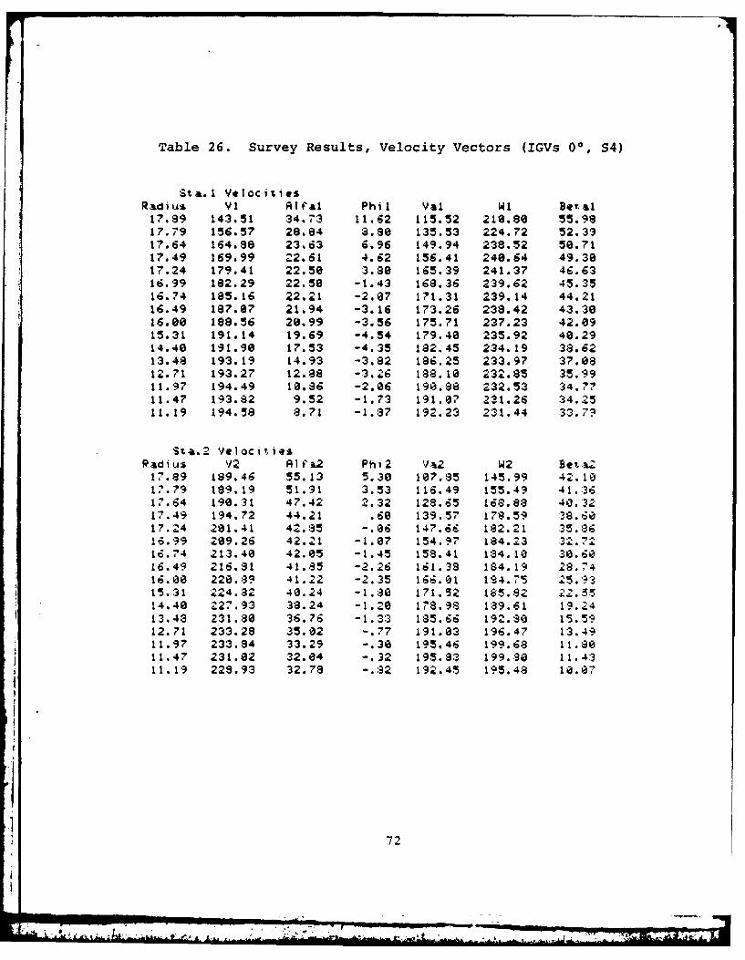
Table 26. Survey Results, Velocity Vectors (IGVs 00, 54)
Sta.1 VelocitiesRad i us VI Altal Phi I Val WI Beta17.89 143.51 34.73 11.62 115.52 218.80 55.9817.79 156.57 28.84 3.90 135.53 224.72 52.3917.64 164.88 23.63 6.96 149.94 238.52 50.7117.49 169.99 22.61 4.62 156.41 248.64 49.3817.24 179.41 22.50 3.80 165.39 241.37 46.6316.99 182.29 22.58 -1.43 168.36 239.62 45.3.516.74 185.16 22.21 -2.87 171.31 239.14 44.2116.49 187.87 21.94 -3.16 173.26 238.42 43.3016.00 188.56 28.99 -3.56 175.71 237.23 42.8915.31 191.14 19.69 -4.54 179.40 235.92 40.2914.40 191.98 17.53 -4.35 182.45 234.19 38.6213.48 193.19 14.93 -3.82 186.25 233.97 37.0812.71 193.27 12.88 -3.26 188.18 232.85 35.9911.97 194.49 10.86 -2.86 190.88 232.53 34.7711.47 193.82 9.52 -1.73 191.07 231.26 34.2511.19 194.58 8.71 -1.37 192.23 231.44 33.73
sta.2 VelocitiesPadi us V2 Rlt'2 Phi2 Va2 W2 Bet, -I.&,17.89 189.46 55.13 5.30 187.85 145.99 42.1017.79 189.19 51.91 3.53 116.49 155.49 41.3617. 64 190.31 47.42 2.32 128.65 168.8$ 40.3217.49 194.72 44.21 .60 139.57 178.59 :38.6017.24 201.41 42.85 -.06 147.61 182.21 35.3616.99 289.26 42.21 -1.07 154.97 184.23 32.7216.74 213.48 42.85 -1.45 158.41 184.10 30.6016.49 216.81 41.85 -2.26 161.38 184.19 28.7416.00 220.39 41.22 -2.35 166.0711 194.75 25.9:315.31 224.82 48.24 -I.30 171.52 185.82 22.5514.40 227.93 38.24 -1.20 178.98 1:89.61 19.2413.43 231.80 36.76 -1.3:3 185.66 192.8 15.5912.71 233.28 35.82 -. 77 191.83 196.47 13.4911.97 233.94 33.29 -.38 195.46 199.68 11.8011.47 231.02 32.04 -.32 195.83 199.88 11.4:311.19 228.93 32.78 -.82 192.45 195.48 18.07
72
I . II' , " - "" -" - -
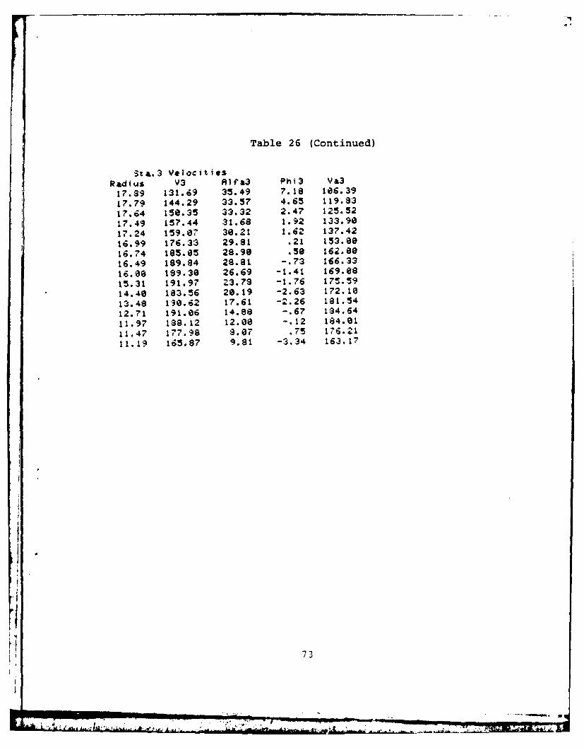
Table 26 (Continued)
ta.3 VelocitiesRadius V3 AI a3 Phi3 Va317.89 131.69 35.49 7.18 106.39
17.79 144.29 33.57 4.65 119.83
17.64 150.35 33.32 2.47 125.52
17.49 157.44 31.68 1.92 133.9017.24 159.07 30.21 1.62 137.42
16.99 176.33 29.81 .21 153.0016.74 185.05 29.90 .50 162.0016.49 189.84 28.81 -.73 166.33
16.00 189.30 26.69 -1.41 169.0815.31 191.97 23.79 -1.76 175.5914.40 183.56 20.19 -2.63 172.1013.48 1,90.62 17.61 -2.26 191.54
12.71 191.06 14.88 -.67 134.64
11.97 188.12 12.88 -. 12 184.0111.47 177.98 9.07 .75 176.21
11.19 165.87 9.81 -3.34 163.17
73
RAL A, NP -,
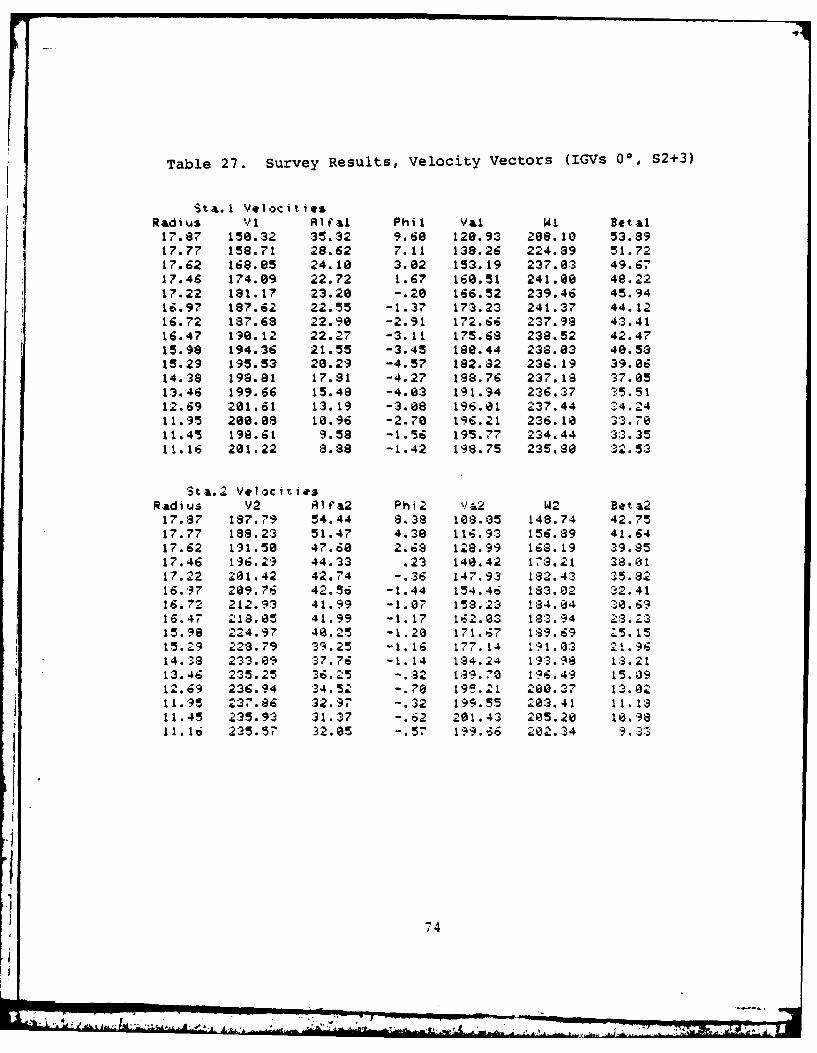
Table 27. Survey Results, Velocity Vectors (IGVs 0*, S2+3)
Sta.1 VelocititsRadius VI ARfal Phil Val Wt Betal17.87 150.32 35.32 9.60 120.93 208.10 53.8917.77 158.71 28.62 7.11 138.26 224.39 51.7217.62 168.85 24.10 3.02 153.19 237.03 49.6717.46 174.09 22.72 1.67 160.51 241.00 48.2217.22 181.17 23.20 -.20 166.52 239.46 45.9416.97 187.62 22.55 -1.37 173.23 241.37 44.1216.72 187.68 22.90 -2.91 172.66 237.98 43.4116.47 190.12 22.27 -3.11 175.68 238.52 42.4715.98 194.36 21.55 -3.45 180.44 238.03 40.5$15.29 195.53 28.29 -4.57 182.32 236.19 39.0614.38 198.81 17.31 -4.27 188.76 237.18 37.0513.46 199.66 15.48 -4.03 191.94 236.37 15.5112.69 201.61 13.19 -3.08 196.01 237.44 24.2411.95 200.08 10.96 -2.70 196.21 236.18 33.7011.45 198.61 9.58 -1.56 195.77 234.44 33.35
11.16 201.22 8.88 -1.42 198.75 235.90 32.53
Sta.* VelocitiesRadius V2 Rlfa2 Phi2 Va2 r- Beta217.87 187.79 54.44 8.38 108.05 148.74 42.7517.77 188.23 51.47 4.30 116.93 156.89 41.6417.62 191.50 47.60 2.68 128.99 168.19 39.8517.46 196.29 44.33 .23 148.42 173.21 38.0117.22 201.42 42.74 -.36 147.93 1:2.43 35.8216.97 209.76 42.56 -1.44 154.46 183.02 32.4116.72 212.93 41.99 -1.07 158.23 134.04 30.6916.47 218.05 41.99 -1.17 162.03 18:3.94 23.Z315.98 224.97 40.25 -1.20 171.67 189.69 Z5.1515.29 2-28.79 39.25 -1.16 177.14 191.8:3 21.9614.38 233.09 137.76 -1.14 184.24 19:3.98 1:8.2113.46 235.25 36.25 -.32 139.79 196.49 15.0912.69 236.94 34.52 -. 70 195.21 200.37 13.0211.95 237.86 :32.97 -. 32 199.55 203.41 11.1811.45 235.93 31.37 -. 62 201.43 205.20 10.9811.16 235.57 32.05 -. 57 199.66 202.34 9.33
74
t - .nil

Table 27 (Continued)
Sta.3 VelocitiesRadiAs V3 R1fa3 Phi3 Va317.87 125.69 33.41 9.26 183.5517.77 144.16 32.25 7.36 120.9217.62 158.74 32.81 2.89 133.2517.46 166.21 31.48 -.59 141.7417.22 169.89 38.36 -.42 146.5816.97 177.87 29.95 -.30 154.1116.72 187.41 29.07 .75 163.7816.47 191.59 28.77 .22 167.9315.98 192.64 25.48 .86 174.8215.29 193.87 24.21 -.82 176.8014.38 192.33 28.26 -1.26 180.3913.46 193.81 16.88 .46 135.4512.69 195.11 14.55 .68 188.8411.95 194.39 11.67 1.89 198.3411.45 188.24 8.31 .28 136.2611.16 173.15 9.66 -2.85 175.'
73
kAI .ILA

Table 28. Off Design Survey Velocity Vectors (IGVs 00, S1)
Sta.1l Velocities
Radius VI RfIal Phil VI WI Betal17.70 183.81 26.63 6.96 163.10 235.32 45.8317.45 193.34 22.96 1.34 177.97 247.09 43.9116.96 206.38 22.93 -1.33 190.03 248.04 39.9716.46 209.71 22.54 -4.24 193.16 246.65 38.2515.97 213.02 21.49 -3.57 197.83 247.37 36.7515.28 216.41 20.01 -4.13 202.82 248.19 34.9814.37 221.91 17.35 -4.62 211.12 252.46 32.9613.44 223.80 15.15 -3.79 215.55 253.06 31.3912.67 224.41 13.13 -3.44 218.15 253.48 30.4411.93 224.23 10.87 -2.48 220.06 253.98 29.8911.44 225.8? 9.43 -2.19 222.66 255.37 29.2411.15 226.97 8.83 -2.13 224.11 255.70 28.70
Sta.2 VelocitiesRadius V2 Alfa2 Phi2 Va2 W2 Beta217.70 199.90 44.51 5.01 142.01 180.42 37.3017.45 208.59 38.89 1.50 162.30 199.42 '35.5016.96 224.38 37.38 -.61 173.28 206.16 30.1416.46 233.48 36.64 -1.31 187.29 209.32 26.4915.97 242.98 36.40 -.98 195.55 211.91 22.6415.28 247.52 35.89 -.66 200.51 212.68 19.4714.37 254.76 34.42 -.80 210.13 218.31 15.7113.44 262.06 33.16 -.24 219.38 224.29 12.0112.67 266.60 31.10 -.65 128'.6 232.06 I0.2911.93 270.32 29.6a -.01 234.86 237.43 3.4411.44 272.36 28.69 -. 01 239.36 241.32 7.3011.15 260.75 28.44 -.81 229.28 231.70 8.29
Sta.3 Velocities
Radius V3 Alfa3 Phi3 VI317.70 161.84 29.16 5.06 140.7917.45 179.14 31.82 1.57 152.1516.96 190.52 28.46 -1.03 167.5716.46 202. S 26.14 -.38 182. 1*
15.97 206.67 2:3.72 -2.39 189.0415.28 211.81 22.47 -.73 195.7114.37 221.50 19.91 .35 208.2613.44 225.39 17.35 .59 215.6012.67 230.37 14.75 1.24 222.7311.93 230.76 16.10 1.41 227.1111.44 218.77 9.19 .69 215.9411.15 202.30 6.40 .25 201.04
76

Table 29. Off Design Survey Velocity Vectors(IGVs 00, 52+3+4)
Sta.1 VelocitiesRadius VI R1lal Phil Val WI Betal17.76 138.29 26.94 8.19 122.83 226.13 56.9617.45 150.31 22.74 4.46 138.21 234.56 53.7716.96 168.17 22.31 2.43 148.05 232.42 58.3916.46 164.97 22.43 -3.03 152.27 228.33 48.1615.97 168.81 21.08 -3.66 156.46 229.06 46.5715.28 169.36 28.00 -4.52 158.65 224.65 44.8914.37 170.42 17.72 -4.53 161.83 222.20 43.8613.44 169.94 15.08 -3.33 163.82 219.71 41.6812.67 170.86 13.32 -3.18 166.80 217.37 48.1612.68 169.97 13.22 -3.46 165.16 217.13 48.3511.93 170.83 10.92 -2.49 166.80 215.67 39.2811.43 169.63 9.57 -1.75 167.19 214.81 33.5911.15 170.95 9.57 -1.69 168.50 212.41 37.47
Sta.2 VelocitiesRadius V2 RAla2 Phi2 V/a2 W2 eta217.78 182.34 56.78 1.05 99.89 139.77 44.3817.45 183.51 48.55 1.19 121.45 163.35 41.9616.96 195.72 45.83 -.86 136.36 168.71 36.8616.46 202.46 45.33 -1.19 142.38 167.71 31.9315.97 287.66 44.34 -1.56 148.46 168.99 28.4915.28 210.73 42.85 -1.53 154.43 170.73 25.2014.37 213.58 48.99 -2.29 161.09 173.11 21.3613.44 214.58 39.62 -2.09 165.17 173.65 17.8612.67 213.90 37.38 -1.47 169.92 176.99 16.1912.68 214.02 37.40 -1.52 169.96 177.8 16.1511.93 211.70 35.64 -1.32 172.01 177.91 14.7511.43 208.94 34.07 -1.45 173.03 178.74 14.4511.15 206.60 35.14 .23 168.94 173.31 12.89
Sta. 3 VelocitiesRadius V3 RIa3 Phi3 Va317.70 123.32 39.55 2.32 95.8117.45 126.31 33.72 .79 105.0516.96 148.87 28.83 3.22 130.2116.46 170.36 29.a5 1.66 149.1615.97 177.27 27.60 1.45 157.0515.28 181.36 26.13 1.46 162.7714.37 178.59 21.62 1.84 165.9413.44 173.80 18.26 .81 165.0212.67 173.44 19.19 1.85 163.7712.68 169.87 16.49 .37 162.811.93 161.99 12.42 -.94 158.1811.43 153.53 8.82 -.64 151.7111.15 128.16 12.60 -7.36 124.04
77

Table 30. Velocity Vectors at Station One
at Three Survey Locations
StI.l YelocIties Port 7Radius VI Alfal Phil Val W1 Betal
17.74 146.73 31.23 7.42 124.42 215.81 54.45
17.49 155.59 25.75 3.S4 139.82 227.70 52.02
16.99 169.35 24.69 .43 153.87 228.47 47.66
16.49 185.22 25.38 -.59 167.34 226.90 42.48
16.00 174.48 24.19 -2.43 158.94 221.68 44.14
15.31 176.19 22.66 -2.a6 162.38 220.03 42.36
14.40 178.68 20.30 -2.79 167.39 219.21 40.14
13.47 179.84 17.69 -2.36 170.24 217.87 38.55
12.71 178.65 15.36 -1,46 172.2i 216.96 37.44
11.96 179.16 13.26 -.51 174.38 216.10 36.28
11.47 179.14 12.11 .05 175.15 214.68 35.33
11.18 180.29 12.12 .38 176.27 213.11 34.28
Sta.1 Velocities Port 8
Radius VI Alfal Phil Iat W1 Betha
17.74 140.41 29.95 9.74 119.90 219.49 56.34
17.49 148.84 29.16 5.12 129.46 217.36 53.37
16.99 158.40 28.90 1.61 138.62 214.07 49.62
16.49 181.51 28.37 -. 79 159.69 216.63 42.50
16.01 178.01 27.22 -2.80 151.00 211.67 44.42
15.32 171.11 24.57 -4.67 155.10 212.93 43.04
14.48 173.99 21.24 -5.03 161.55 214.65 40.93
13.47 175.57 18.31 -4.26 166.22 214.64 .9.05A, % 1 9 2 ..7 5 3 7 .6 0
12.70 176.29 16.12 --3.26 169.08 21:
11.97 177.12 1:3.83 -1.74 171.90 213.49 36.33
11.47 177.90 12.10 -1.77 173.86 213.92 35.60
11.18 178.71 11.93 -1.02 174.83 212.47 34.62
t a.l Velocities Port 9Radius VI AlIal Phi! La! wI Beal
17.74 150.31 31.66 6.12 127.21 214.60 53.40
17.49 162.40 26.61 .25 145.20 226.56 50.14
17.00 173.48 24.59 -.52 157.74 230.12 46.72
16.50 177.68 24.57 -1.67 :61.52 226.59 44.!1
16.01 181.85 24.58 -1.40 165.32 223.36 42.23
15.32 180.79 23.,7 -1.68 165.51 219.10 40.91
14.41 181.13 21.54 -1.35 168.44 217.01 .9.07
13.49 181.81 13.82 -1.45 172.a4 216.64 37.40
12.72 191.66 17.08 .A2 173.65 214.56 35.97
11.97 180.38 14.68 -. 01 174.49 213.56 35.21
11.48 180.21 12.90 ,70 175.65 21:3.71 34.72
11.19 131.91 12.17 .28 177..2 214.22 33.89
78
. -- Al. .' .

PC
.0 0
0~uCI1
cn
0uf
Goa
^4I
5W0
79U

I -IN loll 4
LL.-4J
a 0-IN I Uol .
vif
E4 ~ 0
ILL&I

Fq
Stacking ,Line
IGV . -
Trailing2Edge "
SPI
a. Survey Plane 1 IGV Inlet
........ SP2
b. Survey Plane 2 IGV Exit
Figure 3. Locations of Survey Ports
81

t4
Spa
c. Survey Plane 3 Rotor Exit
TaraVerse
S P4
d. Survey Plane 4 Stator Exit
Figure 3 (Continued)
82

1.2
. x
2 7r*3
X
Figure 4. Performance Parameters vs Flow Rate (IGVs 00)
33
.1 4* I'
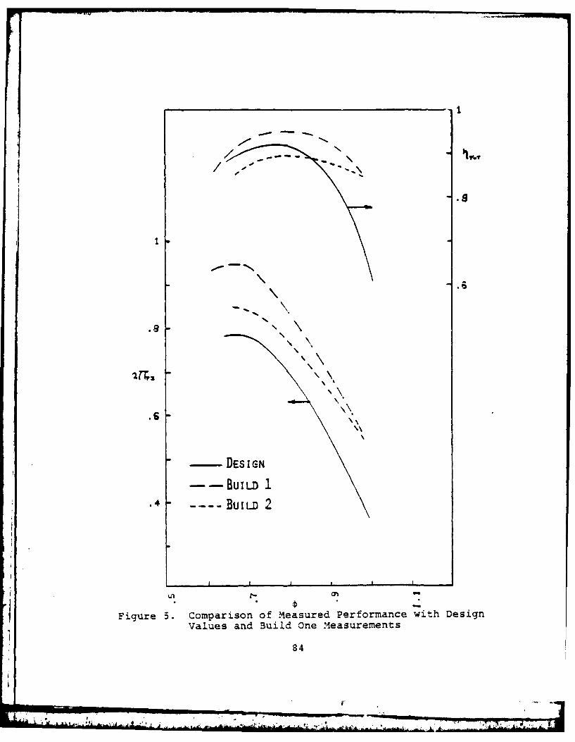
DEIG
-- BUL 1
.4 BULAN
ILL.
-- DEt.G

68
50 0
30
U.
208-.-ig.U*++ + .
+ (
Figure 6.Mid-span Flow Angles vs Flow Rate (IGVs 00)
85
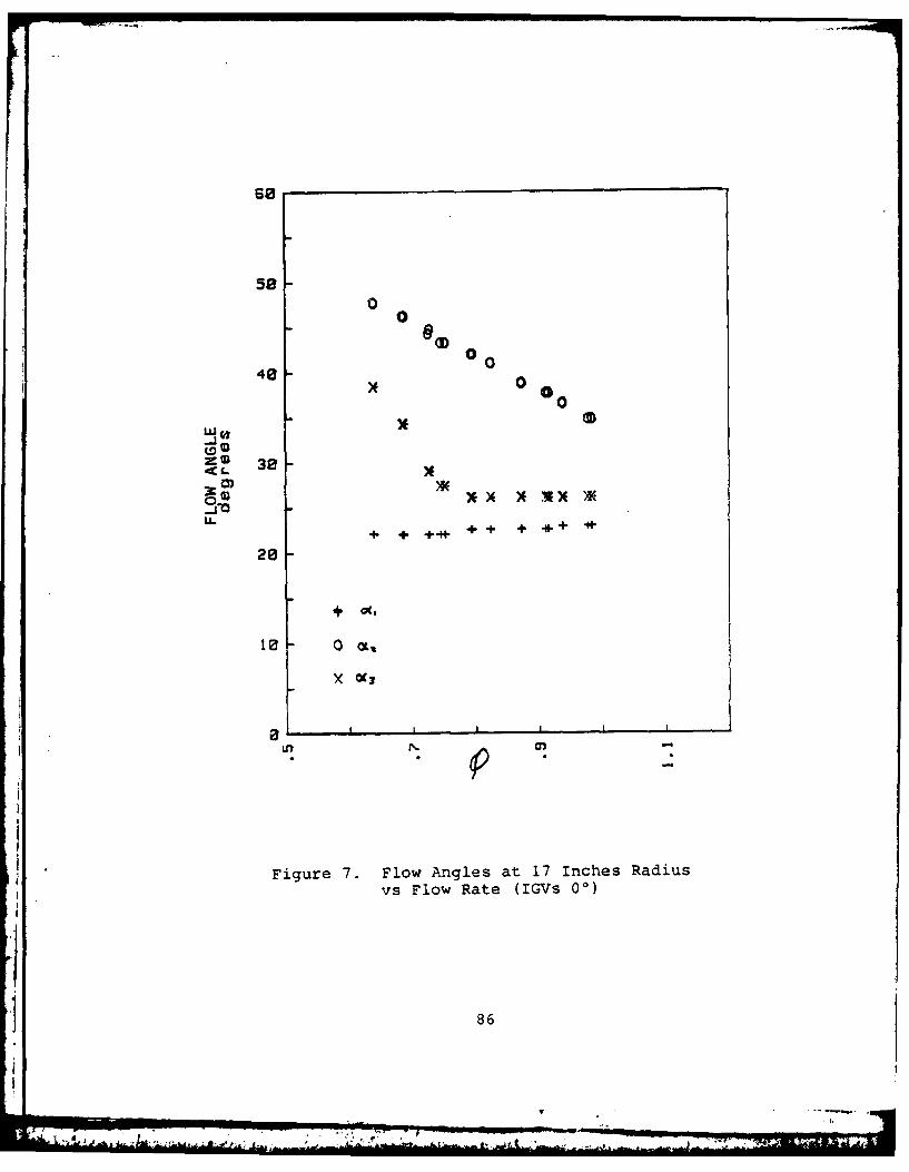
SO
580
0 D
4130 0
-j
9- 308
-M.4. + +* + + .+ +
283
X 0(
Figure 7. Flow Angles at 17 Inches Radiusvs Flow Rate (IGVs 00)
86

TIP
1?1
* S4+5
15.3 ~ J
S EXIT." 14.4
14.4 I-t-INLET
13.5k +• I
12.S I- +
1.7 /
10,1 IHUB
-10 -s -2 2 s 10
TOTAL PRESSUREtnches a4' water
Figure 8. Inlet and Exit Pressure Distributions vs Radius
at Three Throttle Settings (IGVs 00)
87
" i . . _.-
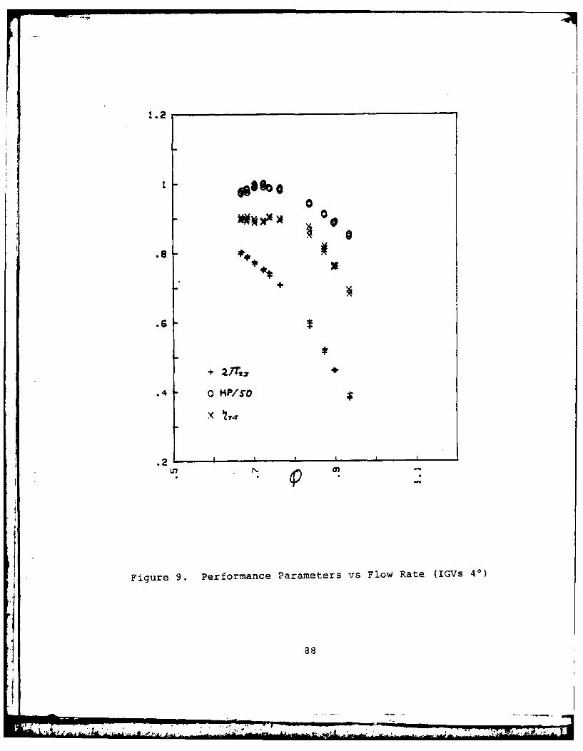
WA 0
.2
a!
Figure 9. Performance Parameters vs Flow Rate (IGVs 40)
5 88

58
48 0 0
3c 00 (0
+oag
x c
Fiue1. Mdsa lwAglsv lwRt I- 0
28 ~ 4.89
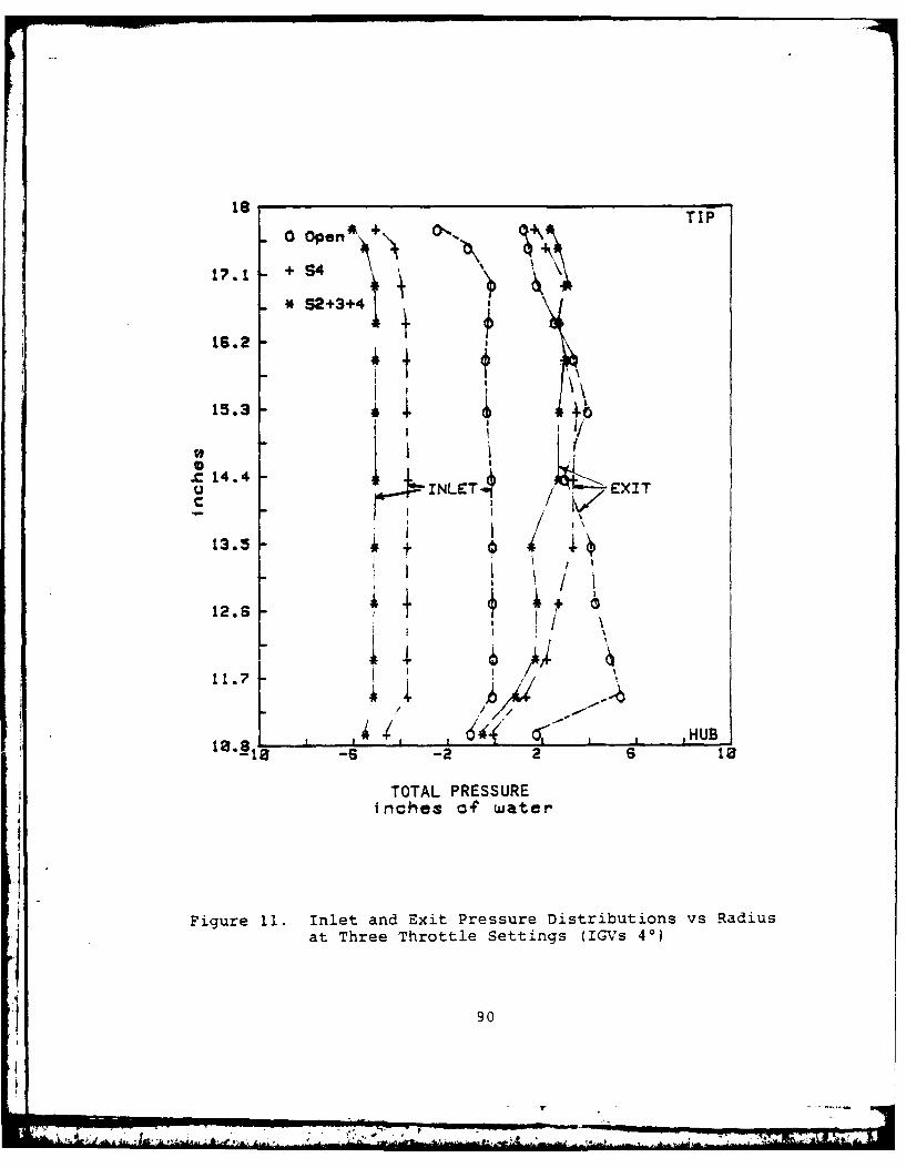
18 TIP
17.1 - +P S4 +
6.2 S2+3+4 ,
. t t15. 0
z14.4 EI
0 INLET EXIT
C
I HU
12.6
Sto
TOTAL PRESSUREinches o.f water
Figure 11. Inlet and Exit Pressure Distributions vs Radiusat Three Throttle Settings (IGVs 40)
90
.4

18 I
'I /TIP
17.1 7/
15.3 1
.C 14.4cC
13.5
1
12.S l
11.7 I
10.8 I ' MUB
FLOW ANGLEde 3 rees
Figure 12. Measured Flow Angle Radial Distributionat Moderate Throttling (IGVs 40, S2+S4;It
Design)
91
9...

ITIP
15.3
7 ,/
- 14.4
c
13.5 /
, i,11.7k 17
18.81 /L I
RELATIVE FLOW ANGLEdegrees
Figure 13. Relative Flow Angle Radial Distributionat Moderate Throttling (IGVs 40, S2+S4;
Design)
92

18
+ V. * Theoregtical Val
17.1 0 Va2.
15.3
0~ 14. %-TheareticalC
- Va2
13.5
112.6
-Ft/sec
Figure 14. Axial Velocity Radial Distribution atModerate Throttling (IGVs 4', S2+S4)
93
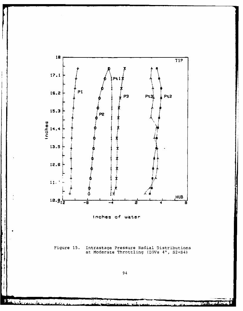
17.1 T I
16.2 Pt1tP3 Pt3 ~Pt2
15.3~ + P-
X" 14.4 -
13.5
12.6k H
12 -8 -4 a 4 a
tnches o water
Figure 15. Intrastage Pressure Radial Distributionsat Moderate Throttling (IGVs 40, S2+S4)
94
-- -- A
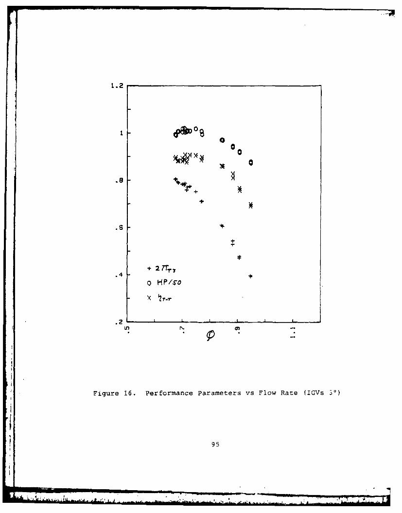
1..2
00
X0
.8 -"
+
.S
+ 27TTr.
0 H P/.go
Figure 16. Performance Parameters vs Flow Rate (IGVs 30)
95

85-A25619 EVLOO F ND HEAPERFORMANCEADAFLOW INAND AACOMPRESSOR U )NDA PST DR ADUD SECHOO MON IEREY CA
IID 0LWADDEL OCT 82 FG 37 NUJNCLt M OSE
M M M S O
MhhhhhhhhhhhhlMMhhMhhhMhhhlMMhhhhMhhhhhhlMflfllflfflfllflffl

10 12 1111122
1.2.5
NATIONAL BRE~AU (If STANDARDS 064COCP RSLTO TETCAR
-_%I
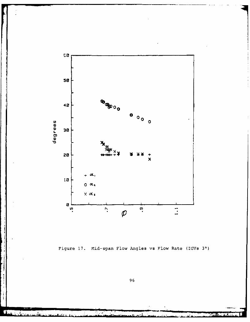
58-
48(
00 0 0 0
3038
Y- 4M x
+tOt
0 Oct
LL
Figure 17. blid-sipan Flow Angles vs Flow Rate (IGVs 31)
96
-om-lll- -- 2- . , -W I . + _ -+.r : -, , ! ~ o , -- - , - | . : _ - -- - . ' . . r r ' " 'T l J _L_ . ' _ " 4

18 TIP
0 Open W+0. +
1?.1 +sI+4
16.2
15.3
I INLET Y"EXIT
." 14.4
C N
13.5 +a /
12.6 + \I I
11.7 -.
-- 6 -2 2 60
TOTAL PRESSURE
inches oae water
Figure 18. Inlet and Exit Pressure Distributions vs Radiusat Three Throttle Settings (IGVs 30)
97
• II I , .. -- " . " - , ....97
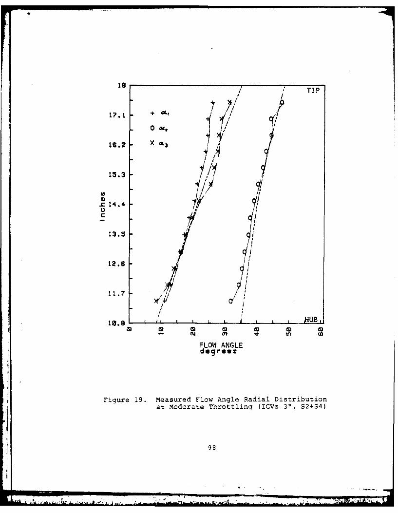
0'0
16.2 X L
15.3 i9.14.4 1
13.51
at MoeaeTrttigUG3, S2S4
98
-T ~ -- ----- - . ...... 7
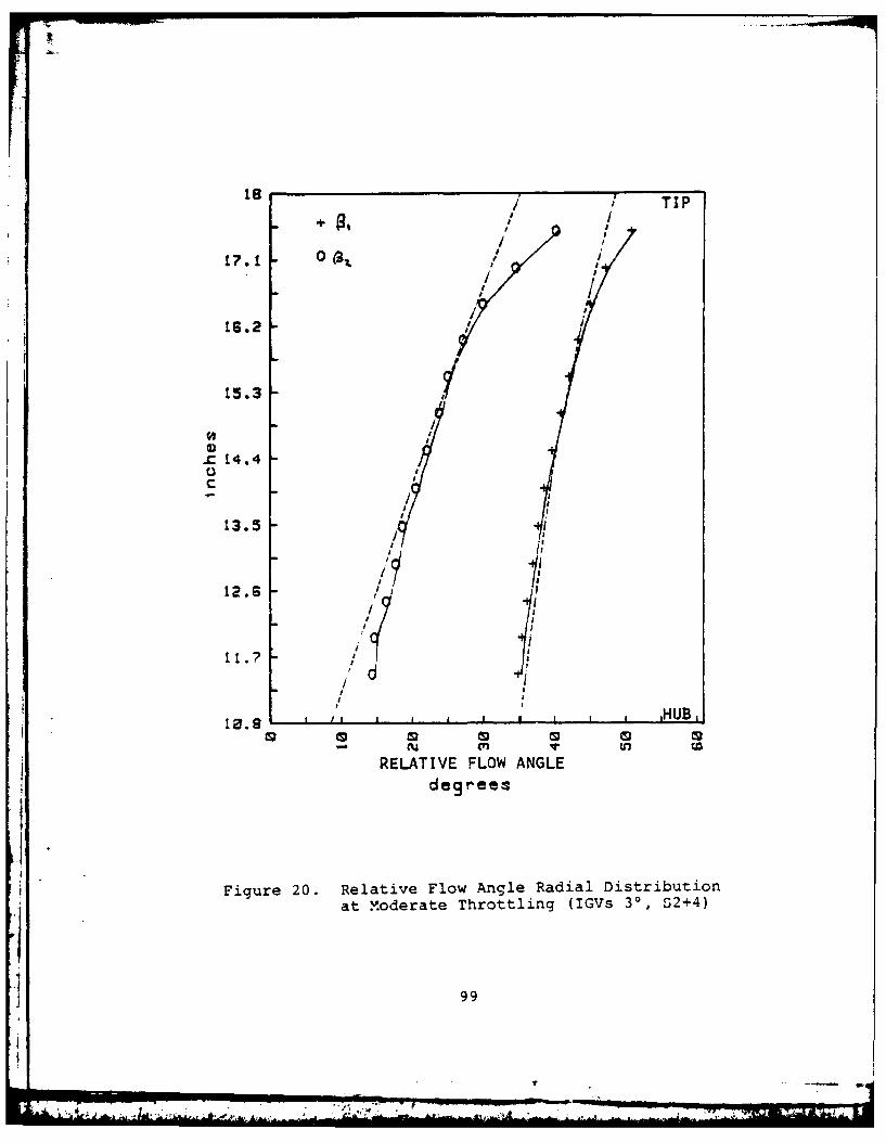
18 1'TIP+I
16.2
15.3/
.C 14.4c
13.5
12.6
15.8HUB,
- cu m (a
RELATIVE FLOW ANGLEdeg rees
Figure 20. Relative Flow Angle Radial Distributionat Moderate Throttling (IGVs 30, S2+4)
99

1, \
17.1 0 Va2 N16.2 X V
15.3
-c 14.4
13.5
12.6
Figure 21. Axial Velocity Radial Distribution atModerate Throttling (IGVs 30, S2+4)
100
r7
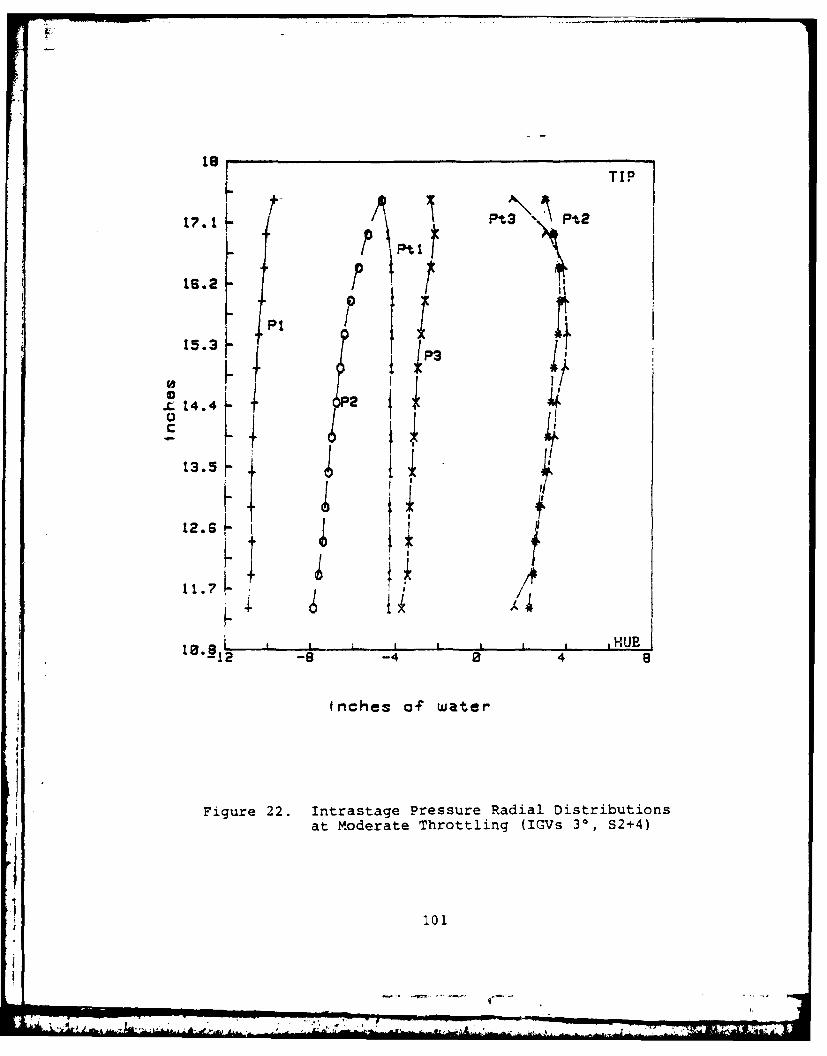
P' 2-TIP
17.1 p3% P.
16.2 - 1
i15.3
.L 1. P
13.5t4
12.S
11.7- V
I I I I I I IIJHUB.12 -8 -4 a 4 B
fnches o? water
Figure 22. Intrastage Pressure Radial Distributionsat Moderate Throttling (IGVs 30, S2+4)
101
-- I J _ i l ' i , m - - . , - "i

1..2
!" 0
+@
+XE~ 2 r-
.4
.8
102
+ 2Tt,.4
o H P/S"o
X r-T
.2 ,
Figure 23. Performance Parameters vs Flow Rate (XGVs 20)
102
:'* , =',.L. • - " - ', ' . , ,~ ~ ~ ~~~. ,,' ' "' ' , . . ., - . .. , ,
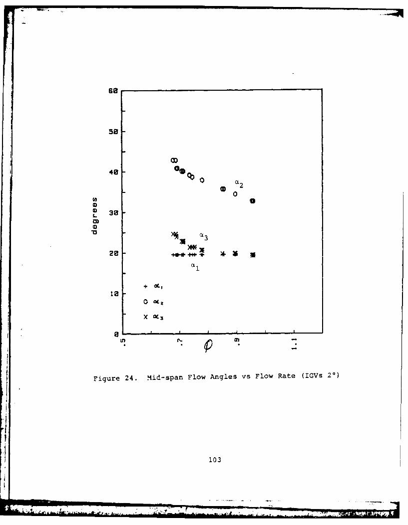
503
48o
40 % (0
300
0 38
LO
~0 OI
28 ~ ~ Of. 4* 3.
110
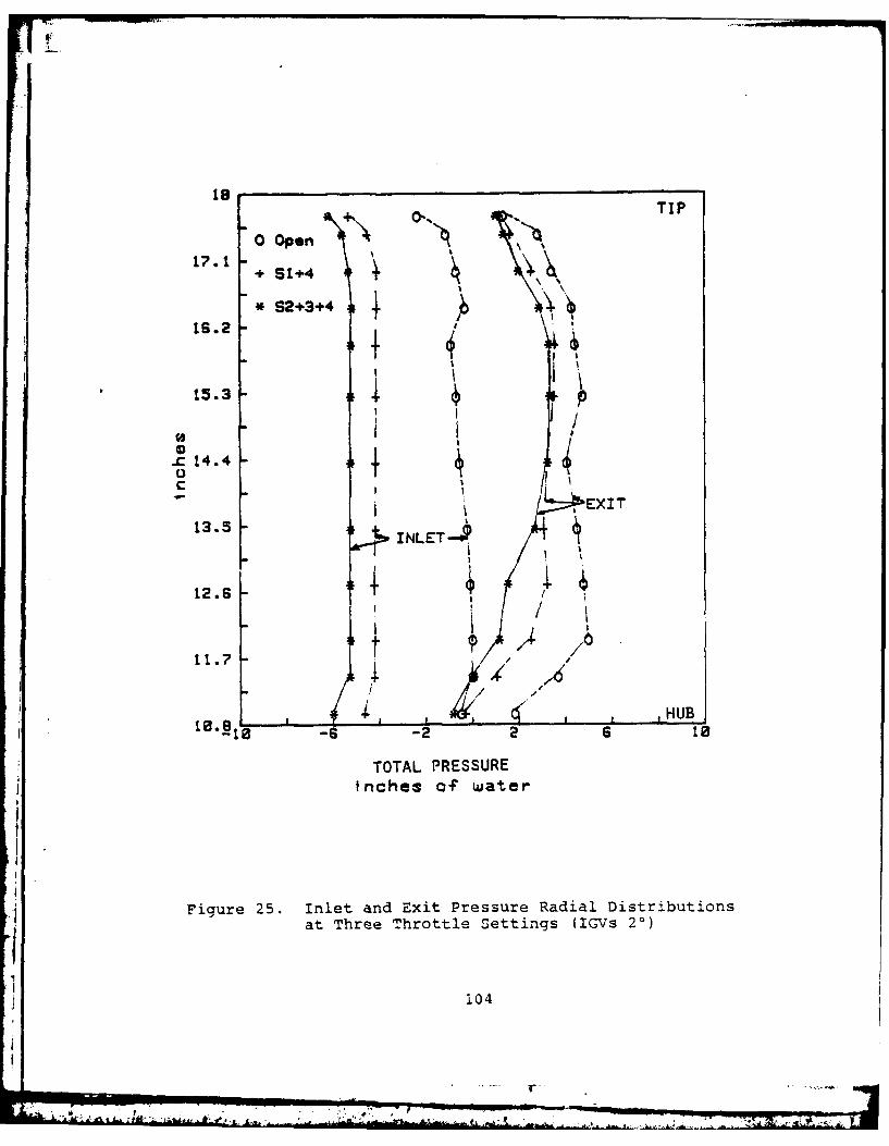
180-.. TIP
0 OpenTI+ S1+4
* S2+g3+416.2 +
I ii115.3 . 4 p
-" 14.4c C ,
1EXIT
13.5 INLET-
HUB1,0._0 8 -6 -2 2 6 10
TOTAL PRESSUREfnches o; water
Figure 25. Inlet and Exit Pressure Radial Distributionsat Three Throttle Settings (IGVs 20)
104
ILL&r
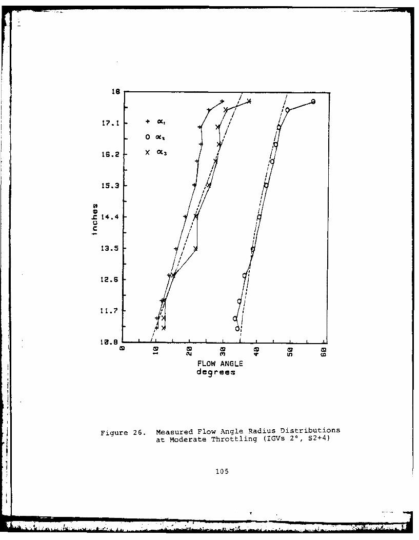
17.1 +
16.2 X M3I
15.3
.14.4
13.5
12.S
11.7
FLOW ANGLEdegrees
Figure 26. Measured Flow Angle Radius Distributionsat moderate Throttling (IGVs 20, S2+4)
105
-4-~-A ___

now. , m
13.5
12.2
11.7
/u m15LTIV FLWANL
10 6

IS.2
.C 14.4
12.S
+ Val.
11.7 0 Va2
X Va3
18.9 L i
-Cuj Cm
Figure 28. Axial Velocity Radial Distributions atModerate Throttling (IGVs 20, S2+4)
107
-- '-A- I

19
17.i P3 Pt
pt I
15.3 . 1
.r 14.4
13.5 LiJ,
I IL!
2.6 StP2 4Pt2
It11.7 /i
0 1
1 8 8~I I I I I I I10.-012 -8 -4 a 4 a
inches o water
Figure 29. Intrastage Pressure Radial Distributionsat Moderate Throttling (IGVs 20, S2+4)
108
I .... I

1 TIP
/
X (X -
//16.2 I
15.3/
.C 14.4
oC
13.5
12.6 -
11.7
8IHUB
FLOW ANGLEdegrees
Figure 30. Measured Flow Angle Radial Distributionsat Moderate Throttling (IGVs 20, S1+4)
109
.--. , - - . -|im

18 TIP+I
17.1 0 i
16.2
15.3
~C 14.4c
13.5/
12.6/
1.1.7
HUB
RELAIVE LOWANGLEdlegrees
Figure 31. Relative Flow Angle Radial Distributions
4 at Moderate Throttling (IGVs 2', S1+4)
- 110
& .6,A .

~'.1 0 4~2
X V..3
15.3
.C 14.40
13.5
U7 U, U7
Figure 32. Axial Velocity Radial Distribution atModerate Throttling (IGVs 2-, S1+4)
A111

+I0,
17.1 I IC
X .
16.2
15.3
.c 14.4 /C
13.5
12.6 /
18.8 I I I , a J I a
CU m V, U11
FLOW ANGLE
degrees
Figure 33. Measured Flow Angle Radial Distributions withClosely Spaced Data Points (IGV 20, S1+4)
112
- -" . *'S - I
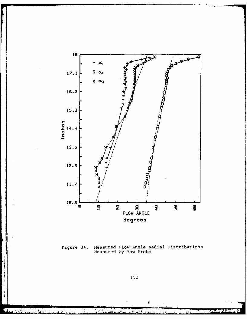
+ '
17.1 Ooc
~14.4/
cu mIin(
11.73

1.2
0 H0
0x~+
.8
.. 1
.4o HP/So
.2 .I,
Figure 35. Performance Parameters vs Flow Rate (IGVs 0O)
114
L4
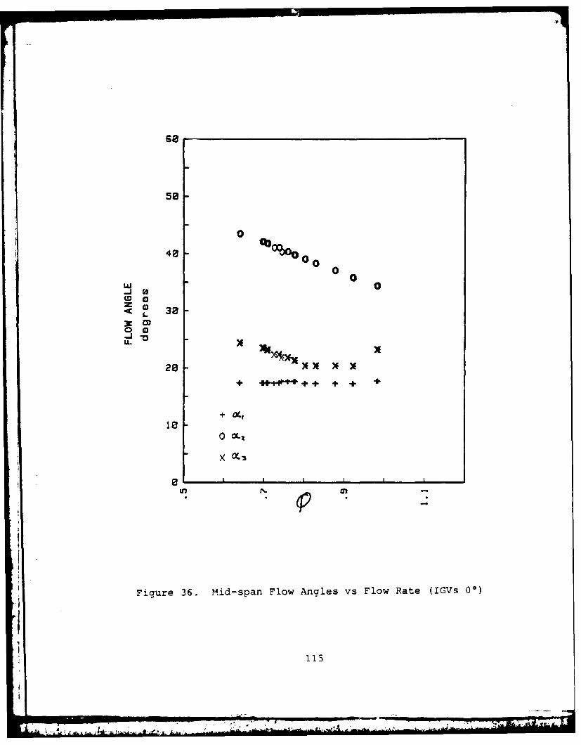
58
0
LU 41 - % 000 00 0
_j 0
300-
(D
+ ~10
o OC.
X O' .3
Figure 36. mid-span Flow Angles vs Flow Rate (IGVs 00)
l's_
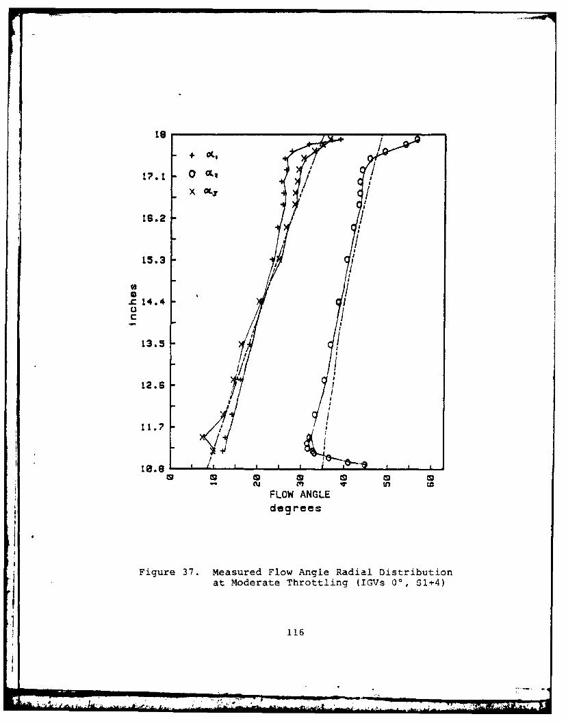
00
cm C" qi
16.16
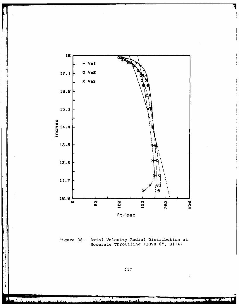
+ Val
17.1 o. I
X V'3\
16.2 -
15.3 !
.C 14.4
C
13.5 -
12.6
11.?,
U, U, 0,
ft/sec
Figure 38. Axial Velocity Radial Distribution atModerate Throttling (IGVs 00, S1+4)
117
4,-- I I L .. , . , , . - - . . . "

WTIP
17.1 Ik ! pt
15.3 P1
.C 4.4
II13.5 .t
12.Pt3 PtI I i
11.7
10. 8 t , k HUB,
'-' -4 4
i nches o; water
Figure 39. Intrastage Pressure Radial Distributionat Moderate Throttling (IGVs 00, S1+4)
118
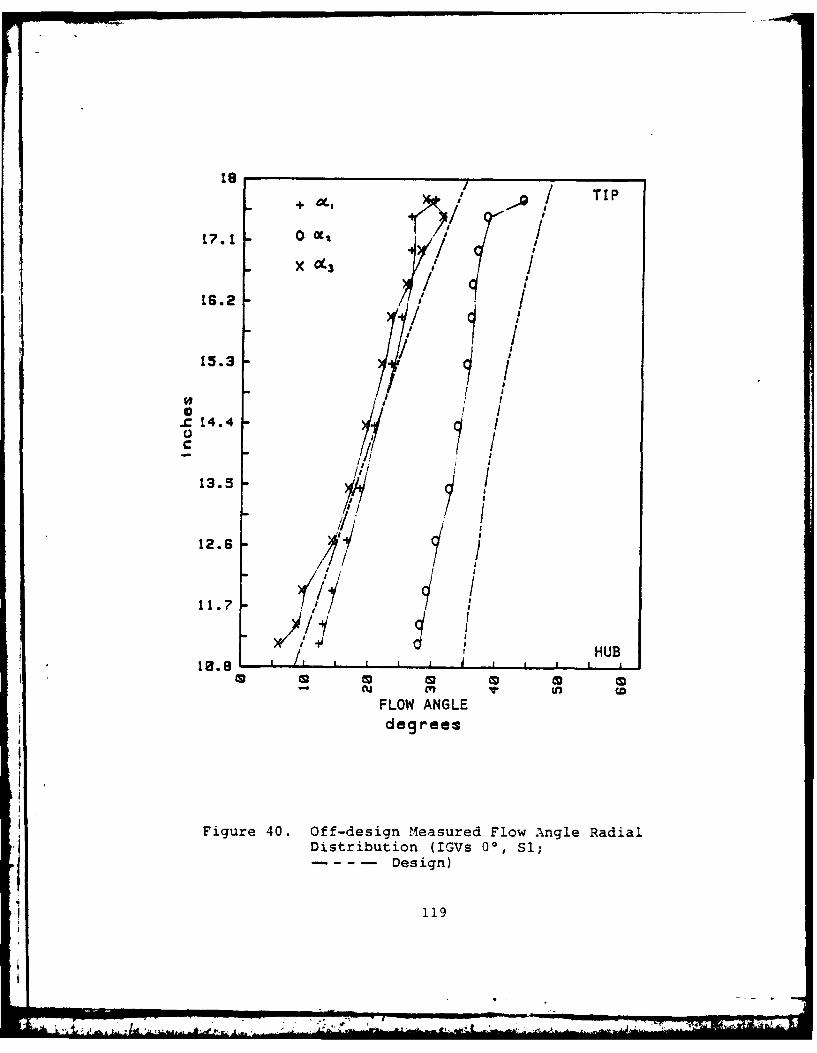
18 /~ I
TI
0I
X (X3/
16.2 ° /15.3 I ,
C 14.41i- a
13.5 : /"
12.6 /I /
11.7 -
HU/ IJ a HUB18.8 a a a I , a a , ,
FLOW ANGLEdegrees
Figure 40. Off-design Measured Flow Angle RadialDistribution (IGVs 00, Si;
Design)
119

18 / / TIP
16.2
15.3
1/
.C 14 .4
a -
13.5 -
If.?12.6S/
I sI
11.7
I 1 I 1HUB,
RELATIVE FLOW ANGLEdeg rees
Figure 41. Off-design Relative Flow Angle RadialDistribution (IGVs 00, 31;
Design)
120
. . .
-- ..
_...i
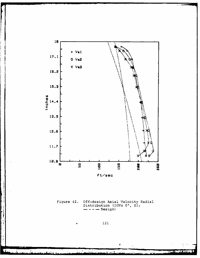
+ Val
1'. 1 0 Va2 \
X Va316.2
15.3
C~ 14.4C
13.5
12.S
11.?
10.9Ln U7,i
f t/Sec
Figure 42. Off-design Axial Velocity PRadialDistribution (IGVs O', Si;
---- Design)
121

It
10*
15.3
pt3
o \
14.4 P2 P3 pt I \pt2
I
13.5 "i4
inches of water
Figure 43. Off-design Intrastage Pressure RadialDistribution (IGVs 00, Si)
122
am. "rag
r ' .
. . . . . . .. . .. . . . . . . .
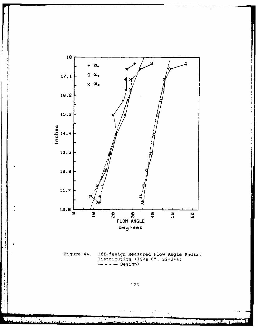
x O( /
16.2
15.3/
-C 14.4
13.5
12.S
11.7 ~
FLOW ANGLEdegrees
Figure 44. Off-design Measured Flow Angle RadialDistribution (IGVs 00, S2+3+4;
- -- -Design)
123
.- , ,

+ to Jo I/V9 III/ i
15.3
///
/ .'
_C 14.4c
13.5 .
/ 17/12.6
18.8 1 1 1 1
cu U7 (a
RELATIVE FLOW ANGLEdeq reez
Figure 45. Off-design Relative Flow Angle RadialDistributions (IGV 00, S2+3+4;
Design)
124
Il.. j .L ; -..... .......-.-.
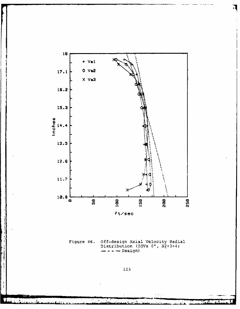
18 \ ,
+ Val \
17.1 0 Va2
. X Va3
16.2
15.3
S
. 14.4
C
13.5
,\\12.6
11.7
II I,
10.8 I I £
-. CU
Ft/sec
Figure 46. Off-design Axial Velocity RadialDistribution (IGVs 00, 32+3+4;
Design)
125
I I4

TIP
16.2 P3 \
15.3 P1 1 ~t6434
CII
I 'I13.5 I
12.6 P2
+ /
1I p i IHUB12-8 -4 a 4 a
inches o€ water
Figure 47. Off-design Intrastage Pressure RadialDistributions (IGV 00, S2+3+4)
126
-"rn ~ I -.L

17.1
16.2'7
15.3
-C 14.4
13.5
12.6 +- SP2 Part?
* SP2 PortS
11.7 if SP2 Ports
10.9-40 cw U
deg rees
-Figure 48. Comparison of Measured Flow Angle at ThreeLocations Relative to the Inlet Guide VaneTrailing Edge (IGVs 30, S2+4;
- -- -Design)
127
r .- ~ . 7F - - V
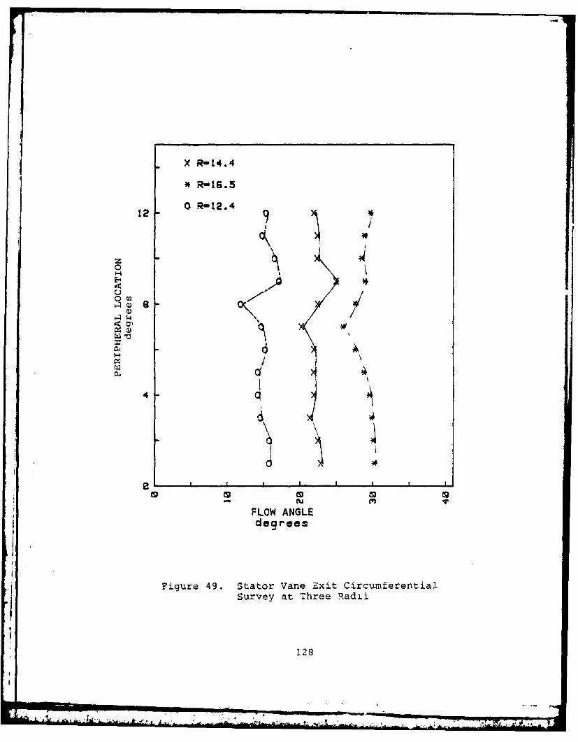
X R- 14. 4
* R- 16. 5
12 0 R- 12. 4
44
4 %
FLOW ANGLEdegrees
4 Figure 49. Stator Vane Exit CircumferentialSurvey at Three Radii
128

TIP
16.2
L5.3
.C 14.4
C
13.5t
12.6PI
10.12I 1HUB12 -10 -e -s -4 -2a
inches o-F water
Ficure 50. Inlet Total Pressure Radial Survey Results
129

. .. 11 rI- I I I I I
i AlX ftA ii l i~ i i ! l J i l
a. Torque Fluctuations
I F I I T I a F lu ai on I I I
I 5 Tua Ilet Ule Pressure Il
'I K T
I I I I I l11 1 L I1TORQUE
"A YtA -t l A! ih A I I . . .k .4 K 1j I- :
! ! 1 I IM ] 1 -f , "
I L Il I 'ki I I I
; FLO RATE' Ii
b. Toqu an Flo Rate Fluctuatio...
Fiur 1. Toqe n Inle'
.:zl PressureFlu:tu ti, ns i t T i, aJ"l ,~
ji t -i j IN - " , ; 1 , ! I, il
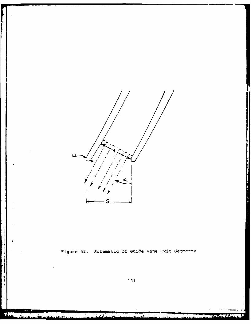
/ ,
/O/t
Figure ~ ~ 52,ceai fGieVn xtGoer
/ / 131
MI"/I ,d/ ,

APPENDIX A
SURVEY PROBE CALIBRATION
The United Sensor five hole probes can be used to mea-
sure three dimensional flow velocity vector, but first they
must be calibrated. All probes used in the present study
were calibrated in-house. The calibration process is de-
scribed in Ref. 12. The probes were inserted in a known
steady, free-jet flow and the pitch angle was varied at
several fixed values of the velocity. Each probe was cali-
brated over a range from 90 to 350 feet per second and over
a pitch angle range of at least -8 to 12 degrees. Probe
pressure readings, pl to p5 , were used to evaluate the two
coefficients
Pl -1 P23 AlS = 1 3A(1)p1
and
P4 - P5- A(2)
P1 - P23
These coefficients are related uniquely to the pitch angle
and the dimensionless velocity, X, defined as
-i- M2
_ V 2 A(3)X - 2 Cp~ t + 1 M2 A3
132
132
4~~~~ ..>. ... ... .. . ...
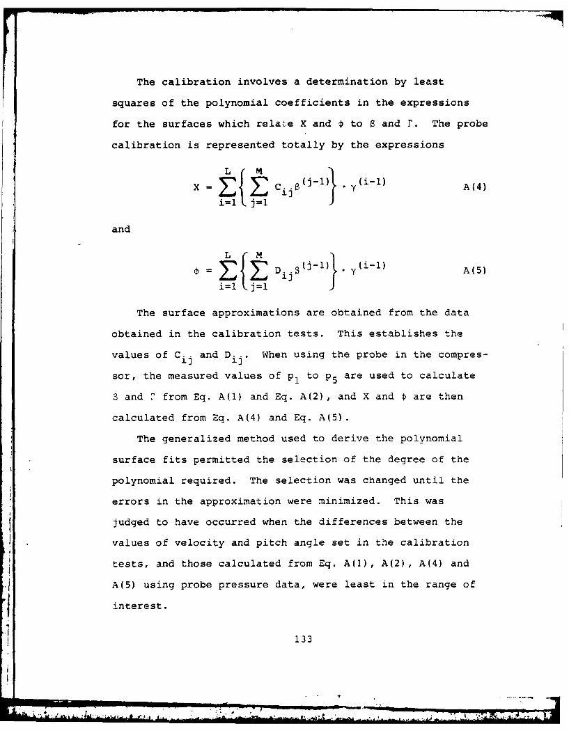
The calibration involves a determination by least
squares of the polynomial coefficients in the expressions
for the surfaces which relate X and to B and r. The probe
calibration is represented totally by the expressions
X E E cijs~-l YA(4)i=l j=l
and
= DijS(J-l) • (i -l ) A(5)i=l lI
The surface approximations are obtained from the data
obtained in the calibration tests. This establishes the
values of Cij and Dij. When using the probe in the compres-
sor, the measured values of p, to P5 are used to calculate
3 and 7 from Eq. A(1) and Eq. A(2) , and X and are then
calculated from Eq. A(4) and Eq. A(5).
The generalized method used to derive the polynomial
surface fits permitted the selection of the degree of the
polynomial required. The selection was changed until the
errors in the approximation were minimized. This was
judged to have occurred when the differences between the
values of velocity and pitch angle set in the calibration
tests, and those calculated from Eq. AM]), A(2), A(4) and
A(5) using probe pressure data, were least in the range of
interest.
133
TF~ .I

The probe coefficients and errors are given in Tables
Al-A3. The three probes are identified by Serial Number
538, Serial Number 539 or "SMITH" (Serial Number unknown).
134
S - ,,--I"L

-W q. LA-4 O N r-
0% o a% qN
Ln a .- Ln
En - LA)4Jr- q. r. r-
q. (V- 0. m 0
-4-4 I.- ON -1 A ~ ~ - - rU) en r- -W -4 00 0
-4*qw mn -W LA 04-4 0 a;I M 1 r- OD I (4-4 '0 r. C14 0 c4 -I r-.0 f
(1 -4 4 (N 047% '.0 M 10 (N 1 00 ()N CNu
ow LA co 0
- . m LA) C1 (N (Vn
x -W C N r, (N e- CD 0 LA) (N M %Dr. - L '.0 LA) m -# r-4 L
E-4 re) v. mN m *
(N 0.0 (N 00 0- I' 0 0 0
C12) 04 I LA as I '.
'-4 '.0 m 00
-4v 4 m NV N 0.0 ~ ~ L r- LC 0 Oq 0 O D r
E-~~r 1- C % *
r- LA CN-4 IV* -4 4.-, (N a%* m
-a; LA (N 9 04 0 LA '0 .
0 ~ ~~~ a% 000"'0 LA L . 1
00 0 f .0 L
C1 MN V. 0
r- (Ti w -4F-- (N 00 e
135
t I- - .9 ' - . - I- ---..

o (4 ()N 0 V M' -4 0 o . m~ m~ r- N~ L O(N %.0-4 m m 0 (N m~ '.0w0 (N '.o(
,-I~~ ~ ~ ~ --4) L 4 -W WL , % 1 0 a
0 4 LA LA r- r- '.0 c LA '. " %0 (N O %D
o n (VI- Ln N O4 -4 () 0 m 0 0 a. wN k.0 LA0 -4'. 4 .-T a 40O- 0 (1- (N -4 0 r- q
cL ces r-0 tn k 0 ( M OD -4 0% OD OD '0
w 0 r- LA (N C14 rI4 0 C4) 0 0 0 C.0 '.0 4o4 .4 .4 (N . 0 LA -. 0 .(N ' . 0 . - . .
.14 N r NO LA ) C.00 OD .D0 4 - LA 0 0 0o1 0 . ND '.0 00 (N 00-40 %D 'g mi m0 (N
-. ' - N r4 -4 0 (N O (3) 4, a~ (N (
ro r- r- k 4 -4) (N N N C) r)0 LO N r", '(f 0 W ( 0 LA4 - (N1 0 '.T LA -4 LA N OC
w- M r- m .D r- Ln C I ( n
4. '0 00 M '.D0 m 0- LA '.0 0 0 0 LA
o LN m .fl- ~ - q. LAO MLAO 0 % L) (N
o (N 0 0 N -4 .-4 .-D 0 a, CN -0 mN 0
04 L 00 NM N M Ln 0 (D -: r-.0) 0 IV~ 0 a0 'T 0 l 0 0 0 0 0 N 4 -
-W' 0 A m 'R 4.1 W I1-4 0
-. ".) 00 LAi (N r4~ 0 C') 4 ( N o A L 00 CD ~ ((n 0 W N
a4 %. %a m %D 1- -W I N w % q
U)U
0 '.0 rn 0 01 r4 0 0 0 (N O 0N .- 4
.- OD a% (n 0' C4 N 0 0 w4. 00 M r-4 ' C4 CD (N
4.)E- -4 0 4*O . q L
aJ c N '. (00I '-4 Wo N 0 '. 07 m (N o-4 U. '.0 -4 '-4 -4 0 n (N4 C%4 N. MN'' 0 e'
1136
0 ~ - '.0~ 0' (N 0'. 0 0 loom -
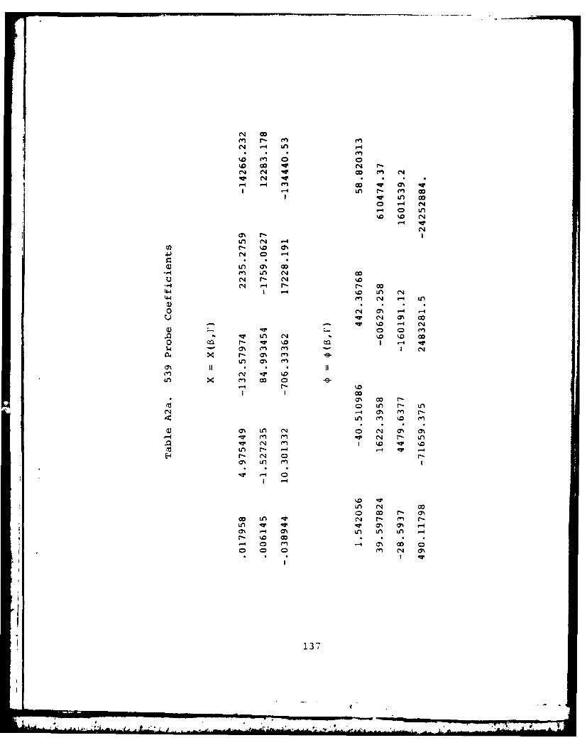
eq -4 In
C4 (NJ qr enqr C4 q.-4 -4 r q 0% q
I 4Ln r- (4 O
0D 1-4 (14- 0 Ul%.0 %D0 CN'
LA N' v-I
U) '. 00rn LN 0
C1 c.J - N4 %Dr-' .-- 0-
L44 In N''0 L44I N) C" -4 LA
C) N~ a4 % 00%D - W ' C14
w - 0 0D rn
o0 r- qw 1.0 .- 4 .q.
x r- ON
00
C) LA r- LACN-4 ON f~ r-
a1 % LA r4 0 ; a;. a;0v-W fn% ?~ r LA
LA3 (N 'n -Wq -
r- CN 0 ra% LA r?)
Lo N 00
'0 00 r
00 ~ ~ Ln N- 0%rn
LIA 4wq qy 0% as -47% -4 0% ULA LA LA n
Z 0. '.0 a;-I 0 CD en C 0N
13 7
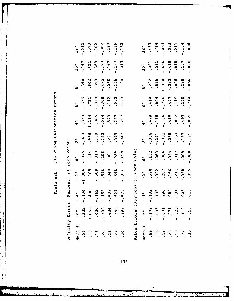
0 lw 4m 0 0 cn N m 0 LA r-4 w w0 -4 m
NO ~-4 C -4 N qr NO- O N '-409-4 6 -
W M~ V-0 0 (0 0 4 0 w0 N w -4 '-4 W0 No, v m Y N r-
4 NO 00 LA w -W 0 40a
-W N m~ LA %00 0 v NW w(0m% 0a m% m m~ 0 a0 w m N m% LA
o M' W M' V 0 -4 r-4 0 N M Mn M' 0 N4 0
$~40 %D~ 0%l CO No % ~0 r, LA V DU.1.4 fn% N4 c O ' LAt n c -4 O N N- r- (0 W -4
5.4 0 r-l 0 M .- 4 0 9-4 0 w ko( N q' r-4 N Nq
-40 UT LA qv Ch N, N, c wD LA N N- 0%4J NOa 0 N, w00 N r ' f m-4 m% 0% 0
0 O N M' 0 LA N4 N4 0 q -4 .- 4 -W 0 :r 40
.- 4
MU M% V0 % -4 LA N- ( -4 r-4 00 N- N- c% 0 N4 %D N, CN r- ON 0(0 % LA a% N
0 M% M -4 -4 N m'~ 0 M N m' Nq r4 r-4 .- 4
w- 0 1LA4 U) qr en 0 -4 ON N0 r. (0 en N a% WoN -4 .-. 4 a00 N LA -4 M' (0 m -400
0 m 0
* 41) (0 LA ch (00 a U oo -v 0 N N- (0 Wqc LA
NN()NLA LAO w09 m LA m9 N .-4 N 0 0
414 1-
IV a C1 nC , nc4a o o o c
E-4 (D 0 0m9 (0 LA ON N- o ( 0 a0% M ON 0 -04 v. v. v m m LAO IV4 r4 -4 N 0 00a0
5-4o Nn NO (9 4 t- Na~ % o -4 0- W ON.4 0 N4 %0 NO W LA Cau c 0 N- M N- N- N -4 LA
<D4 (- 0 N (04 N CD1 C (040 NO-4 0
o~~~~~ .~ .% .9( 09 .O . .~ 0.(400 (
413
Q- -4 . .. .~

00 LA 1-
ON ON q. LAco () ON% LA LA
I-LA r- 0 (14 i.-I-4 LA rn UOl)
N4 N -
LA ONi 0 qrW N-4 00
w-4 w. -WCa LA rn -4
NII ' - 4 0N -W 0) m~ N LA
rq1 4 1 %0 LA q. C-- 00~4-4 (y LA (n e (N4410) 1 d'i C4 ('40 co 14 I- cou 14 en m c
w - r- (rC (
N W - -
(n al0 L Lnq
on 1.0 00 a% m~m
-4N 0 C 0 ('. 1.0
-4 4 N. r40 10 c'4
0' N 00 C--'-4 00'4 (
04 (' 4 0 4o 00 W- co eI I- -4r, 1-
Go ('0 C% '. --
(30 -4 C
139

o (%. w w~ m .Wr Ln 0 Lm LA %.o LA 0 m) ((N 0~O 00 (N - 0 0 01.4*1-4
en LA V m 0 L O . "-4 (N co LA 4 vo 0 mV LA qw %D0 r 0 0 0 4 %D0 r- (7% r4 qr
0 (n0 q NC N 00C 0 C4 r- 9-400D0 0
rn en 0 W~ en -4 4.0 .0 0e LAOw. LA en~ r- V4 0% -l r4i LA -w in 4m
0 LA w. c4 '-4 4- 40 0 (N 1-I4 a 0 -4 1-4
0- O q4 00 qw 00 %0 m~I 00 (7% aC1 -ul (N LA (M (n) 0' %00 ,-.4 LA - 0I ( LAw- 0 Mv M ~ - - -4 r-4 0 0 "14 0 0 .- 0
ON4 I n -4 00 Iw Io r- I0 M In -
( -4 (D co 0 D n0 I) a% LAm LA) a (Na% 4 (n L -4 a% ~ (: nN r, N. (D D-4 04o4 0 1-4.0 (N 00 -4 a N- 000 rn rnOr
.0 1-40 rn Lf 00 r.) 0W 0D r 4 LA i v LAO -w- 0 fn W. -4 '- M 4 0 0 en -a 0 0 4%J 4) -
c I I I
0nLo (M4 0 N ( N ( 4 N L 0 w Ln (N mo4 C4 0 C1 ~ l 0 o, .D - -W) m r4 LA
IV4 0 ) 0 '-4 ('q aN 0- o' 0 4 (N - 0
4-, 0L 0 N. -4 0 .(N -W -W (N (N r0 .0 LA c qr v 0v
140 -4 ON (N0 (N4N L 0 % N .0 M - l l r-) Ln.. - o 0V (N 0 v ( 0 -4-40 ( -40
C., 4J .
E-4
r4a - en '.o 1-4 -40 '.4 -4) o 4 '. O e') ' - CO LAO.0 v 0 OD %.L0 -a WU o %0 r, a%0 a Ln
%. -4 w I( ,
0 Q .0 ( N - - L -4 w .w 00 -4 04 % 0 a. %o C4w 0 '0 rm R% 00 LA 4-4~d'00 4.0 en 0 -n o - 0 00-0 )(N4 00
I4 I I (% I, 4- C4 CA0)
5144
o 00 N N - LA AL,

APPENDIX B
COMPRESSOR DESIGN DATA
The design data for the compressor with symmetrical
blading are given in Table BI and B2 and the calculated off-
design behavior is shown in Fig. 4. Both Table BI and B2
and Fig. 4 are from Ref. 1.
Table Bi. Summary of Mid-span Design Flow Values
Data at MeanRadius, R Vavra Data
mROTOR INLET V* V0.8138al = al/wRm
V* 0.3171ul
W* 0.6829ul
V 0.8734
W1 1.0624
aI 21.288
40.0
L\V Va2/ W* 0.38323
ROTOR EXIT V* V 0.8380a2 a2 /,Rm 0.38
V* 0.7003Vu2W*2 0.2997u2
V* 1.0921V2W* 0.8900w2
39.886
3 2 19.68
141
-- I III ... . . .. "
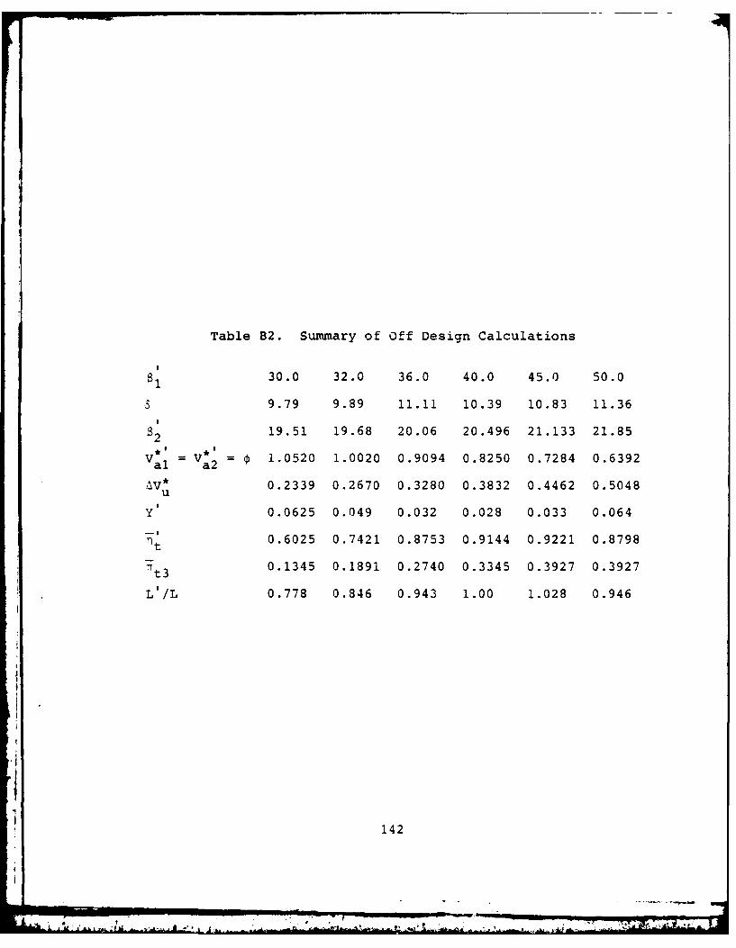
Table B2. Summary of Off Design Calculations
30.0 32.0 36.0 40.0 45.0 50.0
9.79 9.89 11.11 10.39 10.83 11.36
a; 19.51 19.68 20.06 20.496 21.133 21.85
Va1 a2 = P 1.0520 1.0020 0.9094 0.8250 0.7284 0.6392
AV* 0.2339 0.2670 0.3280 0.3832 0.4462 0.5048u
Y 0.0625 0.049 0.032 0.028 0.033 0.064
nt 0.6025 0.7421 0.8753 0.9144 0.9221 0.8798
t3 0.1345 0.1891 0.2740 0.3345 0.3927 0.3927
L'/L 0.778 0.846 0.943 1.00 1.028 0.946
142
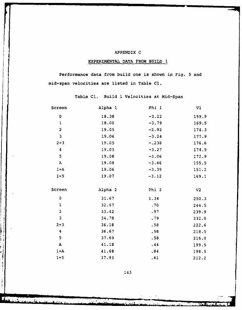
APPENDIX C
EXPERIMENTAL DATA FROM BUILD 1
Performance data from build one is shown in Fig. 5 and
mid-span velocities are listed in Table Cl.
Table Cl. Build 1 Velocities at Mid-Span
Screen Alpha 1 Phi 1 Vi
0 18.38 -3.22 159.9
1 18.00 -3.79 169.5
2 19.05 -2.92 174.3
3 19.06 -3.24 177.9
2+3 19.05 -.238 176.6
4 19.05 -3.27 174.5
5 19.08 -3.06 172.9
A 19.08 -3.46 155.5
1+A 19.06 -3.39 151.2
1+5 19.07 -3.12 169.1
Screen Alpha 2 Phi 2 V2
0 31.67 1.34 250.3
1 32.67 .70 244.5
2 33.42 .97 239.9
3 34.78 .79 232.02+3 36.18 .58 222.6
4 36.67 .58 218.5
5 37.69 .58 216.0
riA 41.18 .44 199.5
1+A 41.68 .84 198.5
~11+5- 37.93 .41 212.2
143

Table Cl (Continued)
Screen Alpha 3 Phi 3 V3
0 20.30 -.01 201.3
1 20.30 -.00 196.9
2 20.30 -.00 193.0
3 19.60 .00 188.9
2+3 19.60 -.00 185.7
4 19.60 .01 182.3
5 19.60 .01 179.6
A 22.20 .01 131.7
1+A 22.20 .01 124.6
1+5 19.40 .01 173.9
144
*1 ..

APPENDIX D
INTEGRATION OF EXIT RAKES
The two total pressure rakes each consisted of twelve
simple pneumatic tubes mounted radially along a common shaft
as shown in Fig. Dl. The distribution of sensors reflects
the relatively even distribution of total pressure expected
over most of the flow channel and the more rapidly changing
conditions expected to occur near the hub and tip. The un-
even radial distribution of sensors made averaging the pres-
sure readings less convenient. Twenty equal flow areas were
defined as shown in Fig. D2 and the value of the pressure
for each of these areas was assigned based on the relevant
probe pressure (Table Dl). From the total pressure, assuming
a uniform static pressure gradient from hub to tip, the rela-
tive mass flows for each area were determined. The mass
flow weighted average total pressure was then calculated
using the relationship
20 E iPti
Pt 20 D(1)
i=2
where mi = A 42o(Pti - P) D(2)
145
• . .

Table Dl. Sub-Area Pressure Determinationfrom Probe Pressures
Pt (1) =((Pt=(1) + Phub) + (Pt(1) + Pt(2)))/3
P t(2) P Pt(2)
Pt (3) = t(3)
P t(4) = (P t(3) + P t(4))/2
P t(5) =P t(4)
Pt (6) = t(4) + Pt(5))/2
Pt (7) = Pt(5) + Pt(6))/2
Pt (9) = Pt (6)
Pt (10) = (Pt(7) + Pt(6))/2
P t(11) = P t(10)
Pt (12) = Pt (7)
Pt (13) = t(7) + Pt(8))/2
P t(14) = P t(8)
Pt(15) = (Pt(8) + Pt(9))/2
Pt(16) = (Pt (9) + Pt(lO))/ 2
P t(17) = Pt (10)
P t(18) = (P t(10) + Pt(11))/2
P t(19) = t(11)
Pt (20) = (Pt (12) + Ptip)/2
146
_ A~l - _ I _ --

ii
T17.5
17.0
I ~
I G.e'
t5.3"
74"
'4.4"
I
O.2~
r~ '-'I '~
Jd
1275
1~* (2.0"
'Is,'
sq
Figure Dl. Total Pressure Rake Geometry
147
* . *, * /~,* ,

ProbeArea *Radius Ports
20 17.855 ~ 119 17.562 "
18 17.26417 16.961 46 10
16 16.653915 16.33914 16.018 - 8
13 15.691
12 15.357 7
11 15.016
10 14.6679 14.309
a 13.9421
7 13.565 po- 5
6 13.177
S 12.777 ~ -4
4 12.365
3 11.938
2 11.4952
1 11.0351
Figure D2. Pressure M1ass Averaging Area Divisions
143
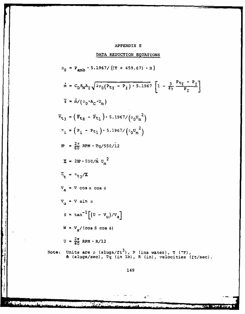
APPENDIX E
DATA REDUCTION EQUATIONS
PO= P amb * 5.1967/ ((T + 459.67) R)
= CD0NAI42po0(P ti - P1 5.1967 1 3 Pt* I p I
= x/(PO*AC*U)
"t3 = (Vt 8 ft ~*j)_ 5.1967/(0 0 U2)
2 7r=P g- RPM 'Tq/550/12
X=21P - 550/m~ U 2
V a V Cosa Cos~
Vu V sin a
=tan- 1 [(U- Vu)/Va]
W -V /(Cos 6Cos)
2wiU = _0RPM. R/12
Note: Units are p (slugs/ft3) P (ins water), T (OF),fit (slugs/sec), Tq (in lb), R (in), velocities (ft/sec).
149
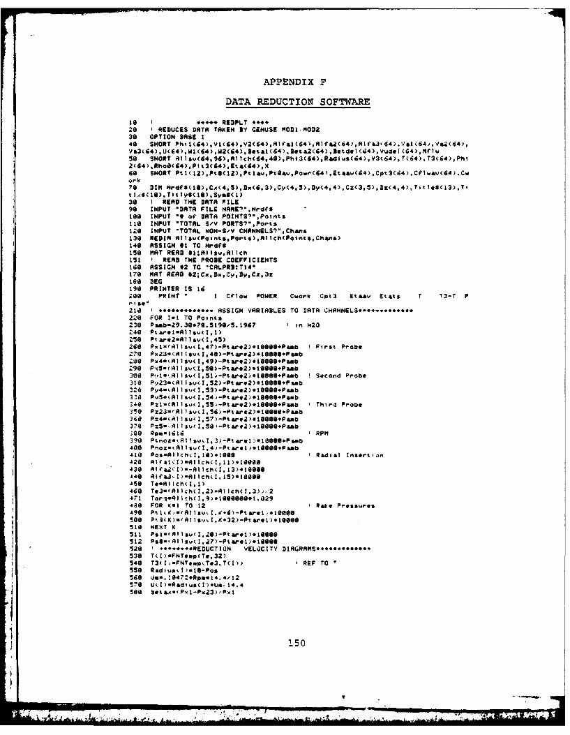
APPENDIX F
DATA REDUCTION SOFTWARE
10 I e*0*c REflPLT ****
20 REDUCES DATA TAKEN BY GENUSE tODI-MOD236 OP TION DASE6I46 SNORT Ph 1(4),V1(64),V2(64),Alea1(64',Al2(64,,Af364,.V1(64,V2(64),Va3.d4),U(64),W1(64),W2(64),3eta1(64),3eta2(64),Betdel(64),VudeI(64),Mflu
156 SNORT Al lsv(64,96),Al lch(44,40),Phl3(64),Radlus(64),V3(64),T(64).T3(64),Phi2(64) ,RhoO(64),Pi t3(64) ,Eta(64),XI so SNORT Pt 1(12) 1PtI( 12) ,Pt 1auPt6kvPour(64) ,Etaau(64 , Cpt3(6;4) .Crl.,ay(64).Cor k70 DIM NrdfS(19),CA(4,S),Dx(6,3),CY~(4,5),Dy(4,4),Cz(3,5),Dz(4.4),Title6C13),Ti
36 READ THE DATA FILE96 INPUT "DATA FILE NAREI",Nrdfs10a INPUT "t of DATA POINTSI",Points116 INPUT 'TOTAL S/v PORTS?',Ports120 INPUT "TOTAL NON-S/V CNANNELS?",Chais136 REDIM Alsu(Points.Ports),Allch(Points,Chais)140 ASSIGN @1 TO NrdfS150 MAT READ *1;AllsvAllch151 1 READ T1HE PROBE COEFFICIENTS160 ASSIGN *2 TO *CALPRB:Tl4*176 MAT READ 02;Cx,Dx,CD,DyiCzDz186 DEG190 PRINTER IS 16206 PRINT - I Cflow POWER Cwork Cpt3 Eta Etats T T3-T P
21a ...... ASSIGN VARIABLES TO DATA CHANNELS-*,********.220 FOR 1.1 TO Points236 Psti.29.36*?6.5196.5.96? Iin H420
.56 Ptar*-2Allsu(1,45)260 PxIIfAllsv(I.4?)-Ptar.2)010666*Paab IFirst Probe279O Px23.(Al lsuI1,49)-Ptare2).lSOS0cPaabZ46 Px4..Allsv(I,49)-Ptare2)41698Paab
30 P'.AlvI5iPte)16SP Stcond Probe
328 PV4- Alls.(I.53)-Ptare2)*10666Paab320 Pu5-R1 lsv(1.54,-Ptage2)el0666c0sb'40 Pz1-(Allsv(1,55 -Ptare2)4100664Paab Third Probe310 Pz23.'Al sv(I,56)-PtareZ)e10696.Paab360 Pz4-tAllsu'I,57)-Ptare2).16666.Paab370 Pz5.,AlIsvtI,56)-Ptare2).16666*Paab80 Rpm-1616 1RPM390 PtnozikA1 suvI.3)-Ptarel)1'e1609Paab4030 PnoZ-(Allsv(1,4j-Ptsse1,*e066Phab4103 Pos.Allch~i.,18)*198 Radial Insertion4260 Is.I-IIh,1.064360 I'2I.Rlc(.3466440 9 h3.,Alh,5e0S459 Te.Allch(1,1)466 Tw3.'AIlch(j,2).A1 lch(I,3)'.'2471 Torq*Al lh(1.9)4106666*I.0294a8 FOR i(.I TO 12 Rake Pressures
506 P 3(K)-ellsv~,I,32)-Ptare1)e166S6
51a NEXT K511 PSlAI s(,6-trl.96512Ps.A sI,7-tr)1S6526 *****.##REDUCTION VELOCITY AC MS.4.4..536 ThI;.FNTemp(Te,32)546 T3I..VTp T*3,T(1). I REF TO T556 RadiuskIl61-Pos560 Umw.10472*Rpm*14.4/I2576 UI)Rdiu*(1)eUm,14.4
150
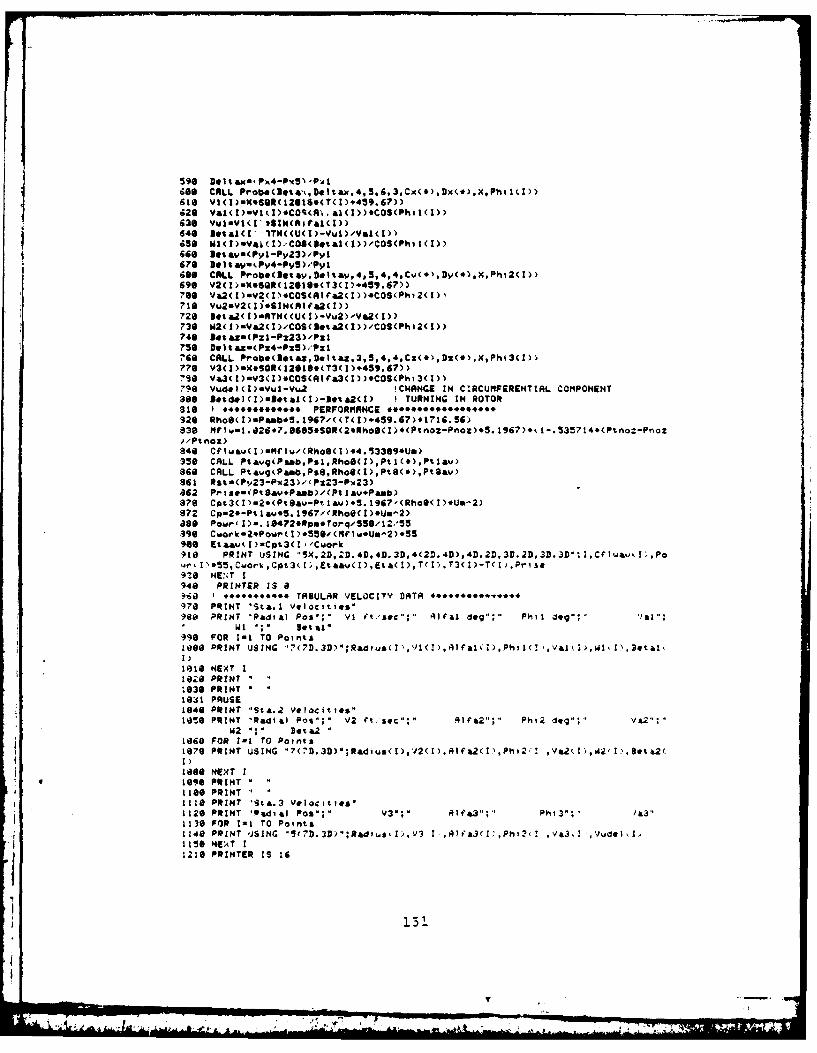
666 CALL Probe(3eta't,Deltax.4,5,6,3,Cic(*),Dx(*),X,Pht 1(I))416 v1(I)uK.SQR(12916.(T(I)+459.67))
646 &.1(1'IT 1(t)(1)-VuI)/VaI(1))
666 vO%&va(PyI-P,23)-PyI
686 CALL Probe(3.tayDeltay,4,5,4,4,Cv(*),Dy(4),X,Pht2(I ))696 V2(1b.X.SQR(12616.CT3C1).459.47))766 Va2(I)3V2(1P.COSCAIfa2(I))4COS(Phl2(1))71: vu2wV2CI)*SIN(Alf&2(I))726 Bot&(I)mATN((U(I-u2)/Y2I))736 k2(I).Va2(I)/COS(3eta2(I))/COS(Pii2(I))746 lotazu(Pzl-Pz23)'Pzt756 DeItaxz4-Px9)iPzl768 CALL Probe(DetazDoltaZ,3,5,4,4,Cz(*),DZ(4),X,Phi3(l))776 VS(1)sX.SGR(12616.(T3(I).459.67))7S@ Va3( I)=3(I ).COS(A1 fa3(I9)).COS(Pi3(I))7'sM Vud&)(Z)euI-Vu2 !CHANGE IN CIRCUMFERENTIAL COMPONENT360 !ed)I.eal1UtZI TURNING IN ROTOR810 ! PERFORMANCE *.*.*..4e326 Rtho(I)sPaab*5.1967'((T(t).459.6?9*1716.56)830 Ifw.I.026.7.68SGR(2.Rho6(I,4(Ptnoz-Pnoz)5.1967)*.1-.5714*(Ptno:-Poz)/Ptnox)846 Cfli.ai(Iflw(co6(I)44.533694U0)350 CALL Ptavg(Paab.Psl,RhoB(I),PtI (.),Ptlav)866 CALL PtawgkPaab,Ps6,RIhO6(I),Ptg(*),PtSav)a61 Rstu(Py23-Px23)-'(Pz^3-Px23)862Pis.PavP)'P aPa)876 CPt3(I).2*(PtSav-Ptlau)45.1967'(Rho6(I)SUS-2)872 Cp.2*-PtlaueS. 19S7/(Rtho(I)*Uan2)a99 Peuvr I)o. 1472*Rpn.Torq'556'12'S55396 Cu.ek2Pow'(I)4S!69'(MflwUm-2)455966 EtaawklI).Cpt3( I 'Cwoik)10 PRINT USING "5X,2D,2D.4D.4D.3D,4(2D.4D),4D.2D,3D.2D,3D.3D'I,Cfla~,I.),Po
P (I*5, Cwor,Cpt3 I ,Etaa,(l) ,Eta( I), P ). T3<1)-T<1I,,Pi-ls.910 HNT I'340 PRINTER IS 0
* iO -4' TABULAR VELOCITY? DATA ... a'.*970 PRINT "Sta.1 Velocities'?80 PRINT "Radial Pos*;" VI ft--soe";" 41lfa1 dog";" Phil dog";*Vl.
WI .;. etasl"?96 FOR lo1 TO Points1098 PRINT USING ?D3);aisI'(,la.)Pi( Y~,1 >3tl
01:3 NEXTI1026 PR INT1630 PRINT1631 PAUSE1646 PRINT 'Sta.2 Velacitios*10SO PRINT Radial Pos";* V2 f-.s~c"' Al f&2";" PhI2 dog";v a,^
W2 Be3t#A21060 FOR 1-1 rO Points1879 PRINT USING "?(7D.3D);Rdius(),02(I).Alfa2(I),Phi2t' ,V&2I,W'i,,3ta2(
I aS0 NEXT I
C1096 PRINT1166 PRINT1lia PRINT Ista.3 volocities,1120 PRINT *Qsdial Pas";" V3';' A 4 &t"; Phi3"" .1,3..1136 FOR 1-1 TO Points
j ~~~~~11 40 PO INT USING -3tD.3D.";R~kdiusi,U3IAi' IPhva.~'"ue..115 NEXT I1216 POINTER IS 16
14, ,k .LA Al --

1211 *..4.* PLOTS OF DATA *.*.**
1226 RAD1236 DISP *FOR PLOTS OF DATA PRESS CONTt249 PAUSE1256 *!*'******t PLOT PERFORNANCE PARAMETERS *.............1260 PLOTTER IS *GRAPHICSO1276 1 PLOTS AXIAL VELOCITY DISTRIBUTION1266 Titl.6 PERFORMANCE1296 TitIx~mwPhi
1300 Titlym* "1316 DATA .5,.4 ,1.2,1.,.1,.I1326 READ Xtm ,Ymin,Xm&x,Ymax,XtIc,YtIc1336 GRAPHICS1346 CALL Sttup(Titl.,TitIxSTitl$YXain,YmlinXaxYmaxXticYtic)1356 Symssu*^1366 CALL Pltr(Sy8l, ,Points.Cflwav(*),Cpt3(*))1376 SmI$'01306 CALL Pit S~mS,1,PoIMIsCflwa *),Poir(.)1396 SamS-"XI140 CALL Pltr(Sym, 1,Polnts,Clwav(4 ,Et aaw())1410 LETTER1426 EXIT GRAPHICS1430 DUMP GRAPHICS1431 PAUSE1446 PLOTTER IS "GRAPHICS"1456 PRINT PAGE1468 I ** ******4 PLOT ANGLES *
1470 TitlIfa*FLOU ANGLES*1469 TitlxSu"Phi "1490 TiIySu~deqreos"150 DATA .5. 6,1.2,66,1,51516 READ Xmin,Ymif,Xmax,Y1maXtic,Ytic152a CALL ,ntcttc).1536 SyoI$8."1540 GRAPHICS1556 CALL Plt,(SvlSl,Points,Cflwav(*),Alal(4).1560 Syu8.'O*1561 CALL P1tcSymS,1,Paln~sCflua,(.),A1¢a2.)15i2 Sy8."X,1565 CALL i vS ,osC1iu., f3j1576 LETTER1580 EXIT CRAPHICS1696 DUMP GRAPHICS161801620 END1636 11640 1 PROBE DATA REDUCTION 3UBROUTINE1650 SUB Proe(B.ta,Delta.C',Cj,DiDj,C*e,Dk.,SHORT X,Phi,1660 OPTION BASE i1676 Gai.-DIt a,/Dta1680 XmFNVeIGmau,B@t&,Ci ,Cj.C(*,)
170 SUBEND1718 1 FUNCTION Vol17:0 DEP FHVelGa,3.,Ci.Cj,Ce)1739 OPTION BASE I
1740 X-01 36 FOR lot TO Ci1760 Too&$1770 FOR Jet TO Cj1 799 Tt IoT*%+C(IJ) Dwl ^fJ-1)
1790 NEXT J130 X0 XT. G-(I-i1818 NEXT I1826 RETURN X1836 FNEND
152
. £ - ,A
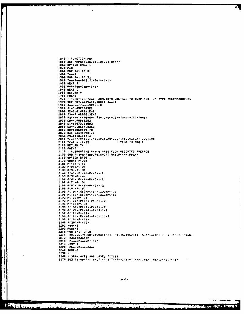
1a8! FUNCTION Phi1850 DIPFN~iGaDIDjD..1860 OPTION BASE I
£67 Pat1660 P0* [at TO Di18"0 ToO1906 FOR Jul TO Dj
1926 MIXT J11930 PuP*TeGam-(I-1,1940 NEXT I1950 RETURN P1966 FNIND1970 1 FUNCTION Tamp CONVERTS VOLTAGE TO TE1NP FOR J' TYPE THERMOCOUPLES1906 DIP FNTemoVoIS,SHORT Junc)1981 Jwnct(Juflc-3z)',1.01990 J105.0373743126" J2*3.0167911IE-22610 23.-?. 42935131-52020 VelsYoI%*I-4*<(J3*Ju,~ct*J2e*Junct*J1)'Junct2630 COS-. 466602522640 C1619073. 1432050 C2.-218614. 53532060 C3wl1569199.702676 C40-264917131.4200 CSw29164413142690 rc.(U(C54V&lC4)4V&1,C3).V&l.C2jeVal.Cl)4Vai.C62166 TfwTc*1.9+32 TEMIP IN DEG F2110 RETURN Tf2120 FNEND2130 1SUBROUTINE Pt avq n~ASS FLOW WEIGHTED AVERAGE2150 SUB Ptayg(Pamb,Ps,SHORT Rho,Pt(*),Pbar)2160 OPTION BASE i21'6 SNORT P(20)2181 P(1).Pt~1)2182 P(2)=P%(2)2183 P(3.-Pt(3)21,34 P(4)u Pt(4)+Pt'3))/22185 PS).Pt(4)
2187 PM7-Pt95)2189 PV8).Pt d)+Pt c5 ,,22189 P(9)-P%(6)2196 P(18..66?,Pt6..333Pt 7)
2192 P(12).P,tK?)2193 P1l3)-'PtC8.'Pt-7)).22194 P(14).Pt-a)2195 P(15)=(Pt~a)*Pt.(9)'.2
2197 P(17).Pt(10)2190 (8.P'18.t1>'2199 P(19a&Pt 11)2286 ;(20);PtkI2)
226 3 PsumuGo2210 FOR lot TO 20
2212 Md tuFtdot *l2213 Psum Psum+P' I)*M2214 NEXT I2220 Pb., ePsumn'Mdot2246 SUBEND
2260 1DRAW AXES AND i-ABEL TITLES
2276) SUB
153
4", -A&_ dU -- A-j
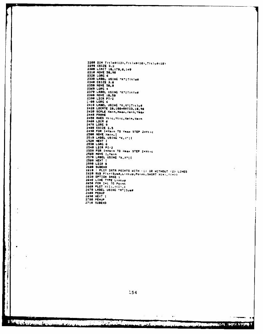
220 DIM Title$(13),Titlx$( 1),TitlyS(1g)2296 CSIZE 3.32306 LIMIT 16,170,,1492310 MOVE 50,902320 LORG 62336 LABEL USING *K";Tit l$2346 CSIZE 3.6
2356 MOVE 50,92360 LOKG 42370 LABEL USING 'K*;TitlxS2366 MOVE 10,562390 LDIR P1/2Z409 LONG 62410 LABEL USING "K,X';Tit1y$2426 LOCATE 26,116*RATIO,14,9e2436 SCALE XetnqXmaxe'amn,Ym&c2446 FRAME2456 AXES XtiCqYtlcXmjnqymi
n2460 LDIR 02476 LONG 82410 CSIZE 2.52496 FOR laYmin TO Ymax STEP 2*Ytic2560 MOVE Xin, I2516 LABEL USING "K.X*:I2520 NEXT I2530 LONG 62546 LDIR PI'22556 FOR IsXmin TO Xmax STEP 2*Xtic2566 MOVE IYmin2570 LADEL USING *K.X-;I2580 NEXT 12596 LDIR 92600 SUBEND2618 6 PLOT DATA POINTS WITH '11 ON WITNOUT (2) LINES2626 SUB Plr(SymS,Liltvp,Point,SHORT X(*),.Y(*))2630 OPTION BASE I2640 LINE TYPE Lintyp
2656 FOR lat TO Point2660 PLOT X(I),f(I),l2670 LABEL USING "R";SvmS268 PENUP2i96 NEXT I270 PENUP2716 SUDEND
2.54
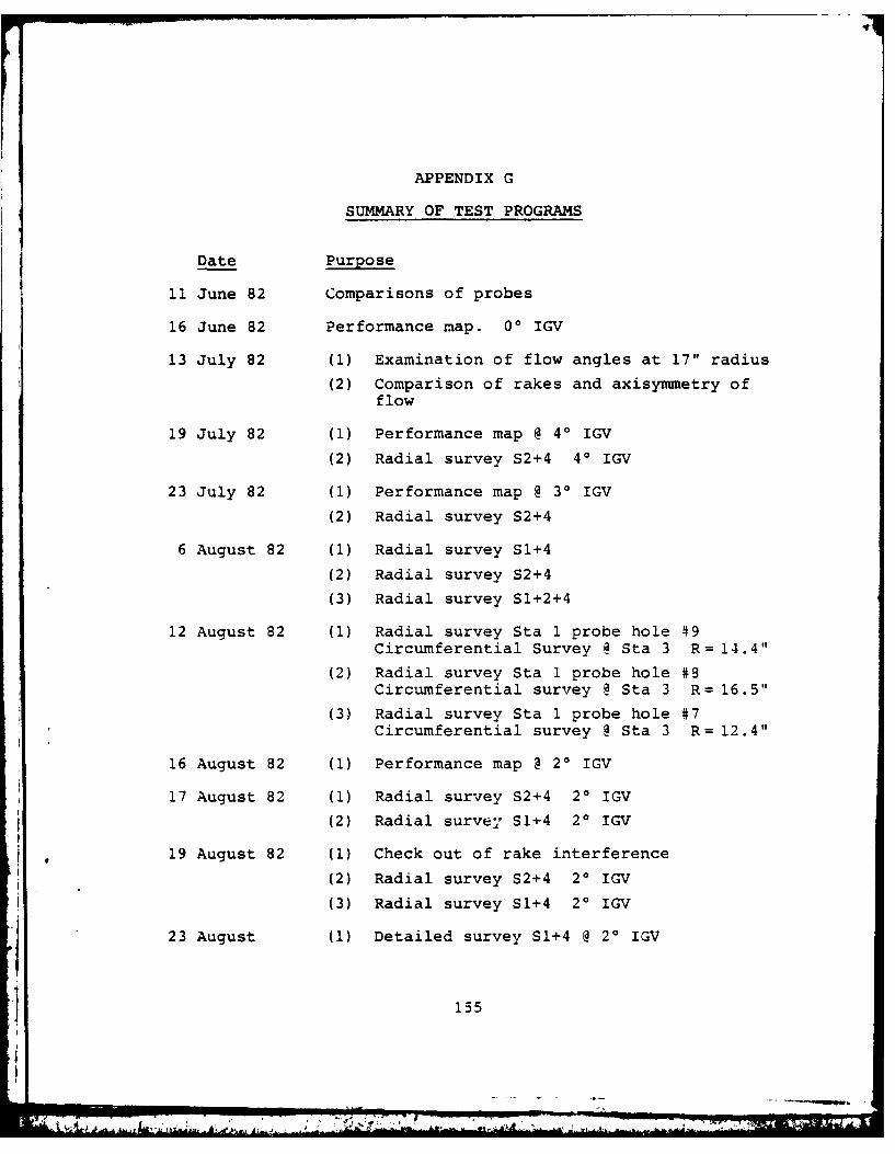
APPENDIX G
SUMMARY OF TEST PROGRAMS
Date Purpose
11 June 82 Comparisons of probes
16 June 82 Performance map. 00 IGV
13 July 82 (1) Examination of flow angles at 17" radius
(2) Comparison of rakes and axisymmetry offlow
19 July 82 (1) Performance map @ 40 IGV
(2) Radial survey S2+4 40 IGV
23 July 82 (1) Performance map @ 30 IGV
(2) Radial survey S2+4
6 August 82 (1) Radial survey S1+4
(2) Radial survey S2+4
(3) Radial survey S1+2+4
12 August 82 (1) Radial survey Sta 1 probe hole 49Circumferential Survey @ Sta 3 R= 14.4"
(2) Radial survey Sta 1 probe hole #9Circumferential survey @ Sta 3 R= 16.5"
(3) Radial survey Sta 1 probe hole #7Circumferential survey @ Sta 3 R= 12.4"
16 August 82 (1) Performance map @ 2* IGV
17 August 82 (1) Radial survey S2+4 20 IGV
(2) Radial survey S1+4 20 IGV
19 August 82 (1) Check out of rake interference
(2) Radial survey S2+4 20 IGV
(3) Radial survey S1+4 20 IGV
23 August (1) Detailed survey S1+4 @ 20 IGV
155

24 August 82 (1) Detailed survey S1+4 @ 20 IGV with
cobra probe Sta 0; with yaw probe Sta 1
26 August 82 (1) Performance map @ 0* IGV
30 August 82 (1) Survey S4
(2) Survey Si+4
(3) Survey S2+3
2 September 82 (1) Off design survey S1
(2) Off design survey S2+3+4
156
=,Id W I
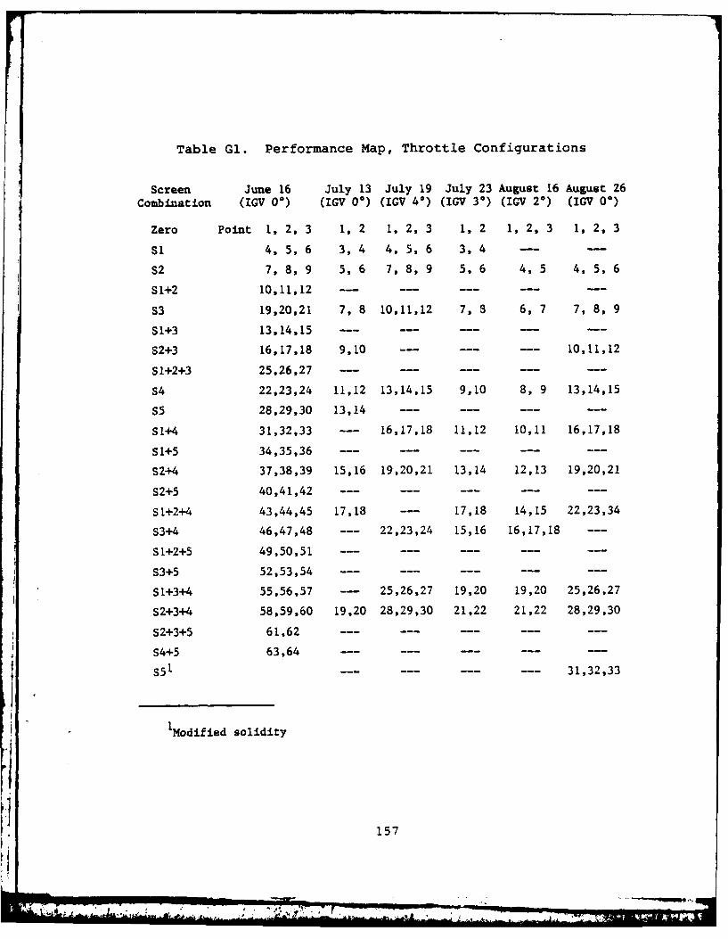
Table Gi. Performance Map, Throttle Configurations
Screen June 16 July 13 July 19 July 23 August 16 August Z6Combination (IGV 00) (IGV 0*) (IGV 40) (IGV 30) (IGV 20) (IGy 00)
Zero Point 1, 2, 3 1, 2 1, 2, 3 1, 2 1, 2, 3 1, 2, 3
Si 4, 5, 6 3, 4 4, 5, 6 3, 4 -- -
S2 7, 8, 9 5, 6 7, 8, 9 5, 6 4, 5 4, 5, 6
S1+2 10,11,12 -- -----
S3 19,20,21 7, 8 10,11,12 7, 3 6, 7 7, 8, 9
S1+3 13,14,15 --------
S2+3 16,17,18 9,10 ------ 10,11,12
S1+2+3 25,26,27 -- -- ---
S4 22,23,24 11,12 13,14,15 9,10 8, 9 13,14,15
S5 28,29,30 13,14 --- - -
SI+4 31,32,33 -- 16,17,18 11,12 10,11 16,17,18
51+5 34,35,36 --- - - -
S2+4 37,38,39 15,16 19,20,21 13,14 12,13 19,20,21
S2+5 40,41,42 -- -----
S1+2+4 43,44,45 17,13 -- 17,18 14,15 22,23,34
S3+4 46,47,48 -- 22,23,24 15,16 16,17,18 -
S1+2+5 49,50,51 -- -- -- --
S3+5 52,53,54 -- -- --- -
S1+3+4 55,56,57 -- 25,26,27 19,20 19,20 25,26,27
S2+3+4 58,59,60 19,20 28,29,30 21,22 21,22 28,29,30
S2+3+5 61,62 -- --- - -
S4+5 63,64----
S51 -- -- 31,32,33
1Modified solidity
157
* Viiillll

LIST OF REFERENCES
1. Naval Postgraduate School Report 57Va73121A, Redesignof the Low Speed Three Stage Axial Flow Compressor TestFacility, by W. Schlachter, P. F. Pucci and M. H. Vavra,1973.
2. Welch, J. K., Experimental Investigation of the Effectsof Tip Clearance and End Losses on Axial CompressorPerformance, M.S. Thesis, Naval Postgraduate School,Monterey, California, 1973.
3. Naval Postgraduate School Report NPS-57Va70091A, Aero-dynamic Design of Symmetrical Blading for Three-StaaeAxial Flow Compressor Rig, by M. H. Vavra, 1970.
4. Turbopropulsion Laboratory, Naval Postgraduate School,Technical Note 80-09, Multistage Compressor--InitialMeasurement with One Stage of Symmetric Blading, byI. N. Moyle, 1980.
5. Turbopropulsion Laboratory, Naval Postgraduate School,Technical Note 80-06, Multistage Compressor--Installa-tion of Cast-Epoxy Blades, by I. N. Moyle and H. Zebner,1980.
6. Turbopropulsion Laboratory, Naval Postgraduate School,Technical Note 82-01, Multistage Compressor--Flow Lossesin Screens and Plates, by J. L. Waddell, 1982.
7. Turbopropulsion Laboratory, Naval Postgraduate School,Technical Note 82-04, GENUSE--General Purpose DataAcquisition Program for the HP 3052/9845A AcquisitionSystem, by W. A. Proses and J. L. Waddell, 1982.
8. Vavra, M. H., Aero-Thermodynamics and Flow in Turbo-machines, Wiley, 1960.
9. Horlock, J. H., Axial Flow Compressors, ButterworthsScientific Publications, 1958.
10. Naval Postgraduate School Report 1174VA1, Axial Turbine
Design Data, by M. H. Vavra, 1974.
11. Turbopropulsion Laboratory, Naval Postgraduate School,Technical Note 81-03, Multistage Compressor--Fabricationof Cast Epoxy Blades, by I. N. Moyle, 1981.
A
12. Turbopropulsion Laboratory, Naval Postgraduate School,Technical Note 82-03, Computer Software for the Cali-bration of Pneumatic and Temperature Probes, by F. Neu-hoff, -1982.
159
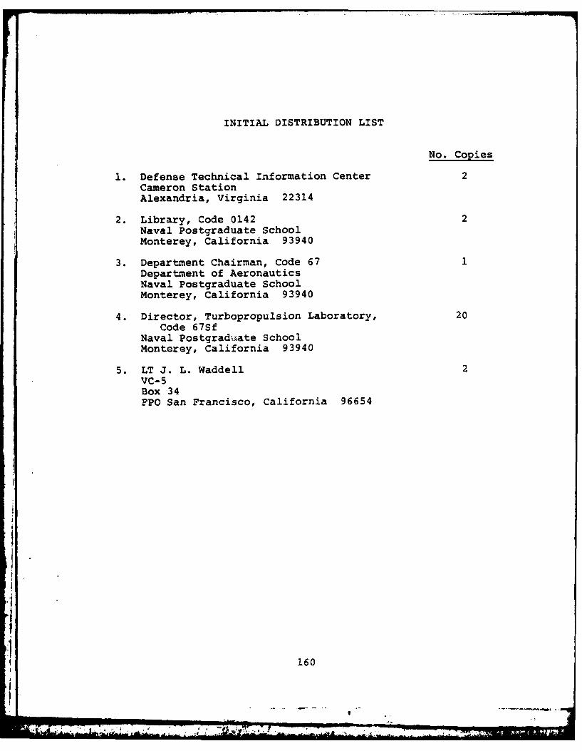
INITIAL DISTRIBUTION LIST
No. Copies
1. Defense Technical Information Center 2Cameron StationAlexandria, Virginia 22314
2. Library, Code 0142 2Naval Postgraduate SchoolMonterey, California 93940
3. Department Chairman, Code 67Department of AeronauticsNaval Postgraduate SchoolMonterey, California 93940
4. Director, Turbopropulsion Laboratory, 20Code 67Sf
Naval Postgraduate SchoolMonterey, California 93940
5. LT J. L. Waddell 2VC-5Box 34FPO San Francisco, California 96654
160
I I I l - j '- i.[ I _ = • , ,- ,r.. .r . - :"Z :. • " .- ... t . -