Embed Size (px)
Citation preview

Performance Bounds in Parameter Estimation
with Application to Bearing Estimation
A dissertation submitted in partial ful�llment of the requirementsfor the degree of Doctor of Philosophy at George Mason University
by
Kristine LaCroix BellB.S. Electrical Engineering, Rice University, 1985
M.S. Electrical Engineering, George Mason University, 1990
Dissertation Director:Prof. Yariv Ephraim
Electrical and Computer Engineering
Spring Semester 1995George Mason University
Fairfax, Virginia

ii
Acknowledgments
I would like to express my gratitude to Professor Harry L. Van Trees for giving me
the opportunity to pursue this work in the C3I Center at George Mason University,
and for his generous support. I have bene�tted greatly from his direction and
encouragement, and from his extensive knowledge of detection, estimation, and
modulation theory, as well as array processing.
I am deeply indebted to Professor Yariv Ephraim, under whose direct supervi-
sion this work was performed. Working with Professor Ephraim has been a very
pro�table and enjoyable experience, and his willingness to share his knowledge and
insight has been invaluable to me.
I am also grateful to Dr. Yossef Steinberg, whose close collaboration I enjoyed
during the year he visited here. Professors Edward Wegman and Ariela Sofer deserve
thanks for serving on my committee, and for reviewing this thesis.
Finally, I thank my husband Jamie, and our daughters, Julie and Lisa, for all
their love, encouragement, and patience.
This work was supported by Rome Laboratories contracts F30602-92-C-0053 and
F30602-94-C-0051, Defense Information Systems Agency contract DCA-89-0001,
the Virginia Center For Innovative Technology grant TDC-89-003, the School of
Information Technology and Engineering at George Mason University, and two
Armed Forces Communications and Electronics Association (AFCEA) Fellowships.

iii
Table of Contents
Acknowledgments iiList of Figures ivAbstract v
1 Introduction 1
2 Bayesian Bounds 62.1 Ziv-Zakai Bounds . . . . . . . . . . . . . . . . . . . . . . . . . . . . . 72.2 Covariance Inequality Bounds . . . . . . . . . . . . . . . . . . . . . . 92.3 Summary . . . . . . . . . . . . . . . . . . . . . . . . . . . . . . . . . 13
3 Extended Ziv-Zakai Bound 153.1 Scalar Parameter with Arbitrary Prior . . . . . . . . . . . . . . . . . 153.2 Equally Likely Hypothesis Bound . . . . . . . . . . . . . . . . . . . . 193.3 Single Test Point Bound . . . . . . . . . . . . . . . . . . . . . . . . . 213.4 Bound for a Function of a Parameter . . . . . . . . . . . . . . . . . . 233.5 M -Hypothesis Bound . . . . . . . . . . . . . . . . . . . . . . . . . . . 263.6 Arbitrary Distortion Measures . . . . . . . . . . . . . . . . . . . . . . 293.7 Vector Parameters with Arbitrary Prior . . . . . . . . . . . . . . . . . 303.8 Summary . . . . . . . . . . . . . . . . . . . . . . . . . . . . . . . . . 36
4 Relationship of Weiss-Weinstein Bound to Extended Ziv-Zakai Bound 38
5 Probability of Error Bounds 42
6 Examples 476.1 Estimation of a Gaussian Parameter in Gaussian Noise . . . . . . . . 476.2 Bearing Estimation . . . . . . . . . . . . . . . . . . . . . . . . . . . . 516.3 Summary . . . . . . . . . . . . . . . . . . . . . . . . . . . . . . . . . 77
7 Concluding Remarks 78
References 81
A Proof of Vector M -Hypothesis Bound 89

iv
List of Figures
1.1 MSE Behavior in nonlinear estimation problems . . . . . . . . . . . . 2
2.1 Valley �lling function. . . . . . . . . . . . . . . . . . . . . . . . . . . 8
3.1 Choosing g(�) for function of a parameter. . . . . . . . . . . . . . . . 253.2 Scalar parameter M -ary detection problem. . . . . . . . . . . . . . . 263.3 Vector parameter binary detection problem. . . . . . . . . . . . . . . 32
6.1 Geometry of the single source bearing estimation problem using aplanar array. . . . . . . . . . . . . . . . . . . . . . . . . . . . . . . . . 52
6.2 Uniform linear array. . . . . . . . . . . . . . . . . . . . . . . . . . . . 566.3 EZZB evaluated with Pierce, SGB, and Bhattacharyya lower
bounds, and Pierce and Cherno� upper bounds for 8-element lineararray and uniform distribution. . . . . . . . . . . . . . . . . . . . . . 58
6.4 Comparison of normalized bounds for 8-element linear array anduniform distribution. . . . . . . . . . . . . . . . . . . . . . . . . . . . 60
6.5 Comparison of normalized bounds for 8-element linear array andcosine squared distribution. . . . . . . . . . . . . . . . . . . . . . . . 62
6.6 Comparison of normalized bounds for bearing estimation with8-element linear array and cosine distribution. . . . . . . . . . . . . . 65
6.7 Square array. . . . . . . . . . . . . . . . . . . . . . . . . . . . . . . . 676.8 Beampattern of 16-element square array. . . . . . . . . . . . . . . . . 686.9 The function f(�) for 16-element square array for SNR=-14 dB. . . . 696.10 Impact of maximization and valley-�lling for 16-element square
array for SNR=-14 dB. . . . . . . . . . . . . . . . . . . . . . . . . . . 716.11 Comparison of normalized vector bounds for 16-element square
array and uniform distribution. . . . . . . . . . . . . . . . . . . . . . 726.12 Beampattern of 16-element circular array. . . . . . . . . . . . . . . . 746.13 The function f(�) for 16-element circular array for SNR=-14 dB. . . . 756.14 Comparison of normalized vector bounds for 16-element circular
array and uniform distribution. . . . . . . . . . . . . . . . . . . . . . 76
A.1 Vector parameter M -ary detection problem. . . . . . . . . . . . . . . 91

Abstract
PERFORMANCE BOUNDS IN PARAMETER ESTIMATION WITHAPPLICATION TO BEARING ESTIMATION
Kristine LaCroix Bell, Ph.D.
George Mason University, 1995
Dissertation Director: Prof. Yariv Ephraim
Bayesian lower bounds on the minimum mean square error (MSE) in estimat-
ing a set of parameters from noisy observations are studied. These include the
Ziv-Zakai, Weiss-Weinstein, and Bayesian Cram�er-Rao bounds. The focus of this
dissertation is on the theory and application of the Ziv-Zakai bound. This bound
relates the MSE in the estimation problem to the probability of error in a binary
hypothesis testing problem, and was originally derived for problems involving a sin-
gle uniformly distributed parameter. In this dissertation, the Ziv-Zakai bound is
generalized to vectors of parameters with arbitrary prior distributions. In addition,
several extensions of the bound and some computationally useful forms are derived.
The extensions include a bound for estimating a function of a random parameter,
a tighter bound in terms of the probability of error in a multiple hypothesis test-
ing problem, and bounds for distortion measures other than MSE. A relationship
between the extended Ziv-Zakai bound and the Weiss-Weinstein bound is also pre-
sented. The bounds developed here, as well as the Weiss-Weinstein and Bayesian
Cram�er-Rao bounds, are applied to a series of bearing estimation problems, in which

vi
the parameters of interest are the directions-of-arrival of signals received by an array
of sensors. These are highly nonlinear problems for which evaluation of the exact
performance is intractable. For this application, the extended Ziv-Zakai bound is
shown to be tighter than the other bounds in the threshold and asymptotic regions.
Chapter 1
Introduction
Lower bounds on the minimum mean square error (MSE) in estimating a set of
parameters from noisy observations are of considerable interest in many �elds. Such
bounds provide the unbeatable performance of any estimator in terms of the MSE.
Furthermore, good lower bounds are often used in investigating fundamental limits of
the parameter estimation problem at hand. Since evaluation of the exact minimum
MSE is often di�cult or even impossible, good computable bounds are sought. The
focus of this dissertation is on the theory and application of such bounds.
Parameter estimation problems arise in many �elds such as signal processing,
communications, statistics, system identi�cation, control, and economics. An im-
portant example is the estimation of the bearings of point sources in array processing
[1], which has applications in radar, sonar, seismic analysis, radio telemetry, tomog-
raphy, and anti-jam communications [2, 3]. Other examples include the related
problems of time delay estimation [4, 5], and frequency o�set or Doppler shift es-
timation [4] used in the above applications as well as in communication systems
[6], and estimation of the frequency and amplitude of a sinusoidal signal [7]. These
are highly nonlinear problems for which evaluation of the exact performance is in-
tractable.
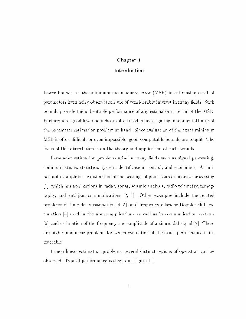
In non-linear estimation problems, several distinct regions of operation can be
observed. Typical performance is shown in Figure 1.1.
1

2
MS
E
ambiguity
region
asymptotic
region
maximum MSE
threshold SNR
Figure 1.1 MSE Behavior in nonlinear estimation problems
In the small error or asymptotic region, which is characterized by high signal-to-
noise-ratio (SNR) and/or long observation time, estimation errors are small. In the
ambiguity region, in which SNR and/or observation time is moderate, large errors
occur. The transition between the two regions can be abrupt and the location of the
transition is called the threshold. When SNR and/or observation time are very small,
the observations provide very little information and the MSE is close to that obtained
from the prior knowledge about the problem. We are interested in bounds which
closely characterize performance in both the asymptotic and ambiguity regions, and
accurately predict the location of the threshold.
The most commonly used bounds are the Cram�er-Rao [8]-[13], Barankin [14],
Ziv-Zakai [15]-[17], and Weiss-Weinstein [18]-[22] bounds. The Cram�er-Rao and
Barankin bounds are local bounds which treat the parameter as an unknown de-

3
terministic quantity, and provide bounds on MSE for each possible value of the
parameter. They are members of the family of local \covariance inequality" bounds
[23, 24], which includes the Bhattacharyya [25], Hammersley-Chapman-Robbins
[26, 27], Fraser-Guttman [28], Kiefer [29], and Abel [30] bounds. The Cram�er-
Rao bound is generally the easiest to compute but is known to be useful only in
the asymptotic region of high SNR and/or long observation time. The Barankin
bound has been used for threshold and ambiguity region analysis but is harder to
implement as it requires maximization over a number of free variables.
Local bounds su�er from the drawback that they are applicable to a restricted
class of estimators, usually the class of unbiased estimators. Restrictions must be
imposed in order to avoid the trivial bound of zero obtained when the estimator
is chosen constant equal to a selected parameter value. Such restrictions, however,
limit the applicability of the bound since biased estimators are often unavoidable.
For example, unbiased estimators do not exist in the commonly encountered situa-
tion of a parameter whose support is �nite [15]. Another drawback of local bounds
is that they cannot incorporate prior information about the parameter, such as its
support. Thus the lower bound may exceed the maximumMSE possible in a given
problem.
The Ziv-Zakai bound (ZZB) and Weiss-Weinstein bound (WWB) are Bayesian
bounds which assume that the parameter is a random variable with known prior
distribution. They provide bounds on the global MSE averaged over the prior dis-
tribution. There are no restrictions on the class of estimators to which they are
applicable, but they can be strongly in uenced by the parameter values which pro-
duce the largest errors.
The ZZB was originally derived in [15], and improved by Chazan, Zakai, and Ziv
[16] and Bellini and Tartara [17]. It relates the MSE in the estimation problem to the

4
probability of error in a binary hypothesis testing problem. The WWB is a member
of a family of Bayesian bounds derived from a \covariance inequality" principle.
This family includes the Bayesian Cram�er-Rao bound [31], Bayesian Bhattacharyya
bound [31], Bobrovsky-Zakai bound [32] (when interpreted as a bound for parameter
estimation), and the family of bounds of Bobrovsky, Mayer-Wolf, and Zakai [33].
The WWB is applicable to vectors of parameters with arbitrary prior distri-
butions, while the ZZB was derived only for a single uniformly distributed random
variable. The bounds have been applied to a variety of problems in [4], [15]-[18],[34]-
[43], where they have proven to be some of the tightest available bounds for all re-
gions of operation. The WWB and ZZB are derived using di�erent techniques and
no underlying theoretical relationship between the two bounds has been developed,
therefore comparisons between the two bounds have been made only through com-
putational examples. The WWB tends to be tighter in the very low SNR region,
while the ZZB tends to be tighter in the asymptotic region and provides a better
prediction of the threshold location [18, 43].
In this dissertation we focus on Bayesian bounds. The major contribution is
an extension of the ZZB to vectors of parameters with arbitrary prior distribu-
tions. Such extension has long been of interest especially in the array processing
area [18, 44], where the problem is inherently multidimensional and not all priors
may be assumed uniform. The theory of the extended Ziv-Zakai bound (EZZB) is
investigated, and several computationally useful forms of the bound are derived, as
well as further extensions including a bound for estimating a function of a random
variable, a tighter bound in terms of the probability of error in anM -ary hypothesis
testing problem for M � 2, and bounds on distortion measures other than MSE.
The relationship between the Weiss-Weinstein family of bounds and the extended

5
Ziv-Zakai bound is also explored, and a new bound in the Weiss-Weinstein family
is proposed which can also be derived in the Ziv-Zakai formulation.
The bounds developed here are applied to a series of bearing estimation problems.
Lower bounds on MSE for bearing estimation have attracted much attention in
recent years (see e.g. [36]-[56]), and the emphasis has been mainly on the Cram�er-
Rao and Barankin bounds. In the bearing estimation problem, the parameter space
is limited to a �nite interval and no estimators can be constructed which are unbiased
over the entire interval, therefore these bounds may not adequately characterize
performance of real estimators. The ZZB has not been widely used due to its
limitation to a single uniformly distributed parameter. In the examples, we compute
the EZZB for arbitrarily distributed vector parameters and compare it to the WWB
and Bayesian Cram�er-Rao bound (BCRB). The EZZB is shown to be the tightest
bound in the threshold and asymptotic regions.
The dissertation is organized as follows. In Chapter 2, the parameter estimation
problem is formulated and existing Bayesian bounds are summarized. In Chapter
3, extension of the Ziv-Zakai bound to arbitrarily distributed vector parameters
is derived. Properties of the bound are discussed and the extensions mentioned
earlier are developed. In Chapter 4, the relationship of the EZZB to the WWB
is explored. In Chapter 5, probability of error expressions and bounds which are
needed for evaluation of the extended Ziv-Zakai bounds, are presented. In Chapter
6, the bounds are applied to several bearing estimation problems and compared with
the WWB and BCRB. Concluding remarks and topics for further research are given
in Chapter 7.

Chapter 2
Bayesian Bounds
Consider estimation of a K-dimensional vector random parameter � based upon the
noisy observation vector x. Let p(�) denote the prior probability density function
(pdf) of � and p(xj�) the conditional pdf of x given �. For any estimator, �̂(x), the
estimation error is � = �̂(x)� �, and the error correlation matrix is de�ned as
R� = En��T
o: (2.1)
We are interested in lower bounding aTR�a, for any K-dimensional vector a. Of
special interest is the case when a is the unit vector with a one in the ith position.
This choice yields a bound on the MSE of the ith component of �.
The minimumMSE estimator is the conditional mean estimator [31, p. 75]:
�̂(x) = E f�jxg =Z�p(�jx)d� (2.2)
and its MSE is the greatest lower bound. The minimumMSE can be very di�cult or
even impossible to evaluate in many situations of interest, therefore good computable
lower bounds are sought.
Bayesian bounds fall into two families: the Ziv-Zakai family, which relate the
MSE to the probability of error in a binary hypothesis testing problem, and the \co-
variance inequality" or Weiss-Weinstein family, which are derived using the Schwarz
inequality.
6

7
2.1 Ziv-Zakai Bounds
This family includes the original bound developed by Ziv and Zakai [15], and im-
provements by Seidman [4], Chazan, Zakai, and Ziv [16], Bellini and Tartara [17],
and Weinstein [57]. Variations on these bounds may also be found in [58] and [59].
They all relate the MSE in the estimation problem to the probability of error in a
binary hypothesis testing problem and were derived for the special case when � is
a scalar parameter uniformly distributed on [T0; T1]. The Bellini-Tartara bound is
the tightest of these bounds. It is based upon the relation [60, p. 24]:
�2 =Z 1
0
�
2Pr�j�j � �
2
�d� (2.3)
and Kotelnikov's inequality [6]:
Pr�j�j � �
2
�� 2
T1 � T0V
(Z T1��
T0
Pmin(�; � +�)d�
); (2.4)
where Pmin(�; � + �) is the minimum probability of error in the binary hypothesis
testing problem
H0 : �; Pr(H0) =12 ; x � p(xj�)
H1 : � +�; Pr(H1) =12 ; x � p(xj� +�);
(2.5)
and V f�g is the \valley-�lling" function illustrated in Figure 2.1. For any function
f(�), V ff(�)g is a non-increasing function of � obtained by �lling in any valleys
in f(�), i.e. for every �,
V ff(�)g = max��0
f(� + �): (2.6)
Combining Eqs. (2.3) and (2.4), the Bellini-Tartara bound on MSE is:
�2 �Z T1�T0
0
�
T1 � T0V
(Z T1��
T0
Pmin(�; � +�)d�
)d�: (2.7)
If valley-�lling is omitted, the weaker bound of Chazan-Zakai-Ziv [16] is obtained.

8
h
f(h)
ν{f(h)}
Figure 2.1 Valley �lling function.
Weinstein [57] derived an approximation to (2.7) in which the integral over � is
replaced by a discrete sum:
�2 � maxf�igri=1
rXi=1
�2i ��2
i�12(T1 � T0)
Z T1��i
T0
Pmin(�; � +�i)d� (2.8)
where 0 = �0 < �1 < � � � < �r � T1 � T0. Although (2.8) is weaker than (2.7) for
any choice of the test points f�igri=1, it can be tighter than the Chazan-Zakai-Ziv
bound, and is easier to analyze. When a single test point is used (r = 1), the bound
becomes
�2 � max�
�2
2(T1 � T0)
Z T1��
T0
Pmin(�; � +�)d�; (2.9)
which is a factor of two better than the original Ziv-Zakai bound [15].
These bounds have been shown to be useful bounds for all regions of operation
[4],[15]-[17], [34]-[38],[43], but their applicability is limited to problems involving a
single, uniformly distributed parameter, and to problems in which the probability
of error is known or can be tightly lower bounded.

9
2.2 Covariance Inequality Bounds
Bounds in this family include the MSE of the conditional mean estimator (the
minimum MSE), and the Bayesian Cram�er-Rao [31], Bayesian Bhattacharyya [31],
Bobrovsky-Zakai [32], Weiss-Weinstein [18]-[22], and Bobrovsky-Mayer-Wolf-Zakai
[33] bounds. Using the Schwarz inequality, Weiss and Weinstein [18]-[22] showed
that for any function (x; �) such that E f (x; �)jxg = 0, the global MSE for a
single, arbitrarily distributed random variable can be lower bounded by:
�2 � E2f� (x; �)gEf 2(x; �)g : (2.10)
The function (x; �) de�nes the bound. The minimumMSE is obtained from:
(x; �) = E f�jxg � �: (2.11)
The Bayesian Cram�er-Rao Bound is obtained by selecting
(x; �) =@ ln p(x; �)
@�; (2.12)
which yields the bound [31, p. 72]:
�2 � J�1
J = E
8<: @ ln p(x; �)
@�
!29=; = �E
(@2 ln p(x;�)
@�2
): (2.13)
In order to evaluate this bound, the joint distribution must be twice di�erentiable
with respect to the parameter [31, 18]. This requirement can be quite restrictive as
the required derivatives will not exist when the parameter space is a �nite interval
and the prior density is not su�ciently smooth at the endpoints, such as when the
parameter is uniformly distributed over a �nite interval.
Bobrovsky, Mayer-Wolf, and Zakai generalized the BCRB using a weighting func-
tion q(x; �):
(x; �) = q(x; �)@ ln [p(x; �)q(x; �)]
@�: (2.14)

10
Appropriate choice of q(x; �) allows for derivation of useful bounds even when the
derivatives of the density function do not exist.
The Bobrovsky-Zakai bound uses the �nite di�erence in place of the derivative:
(x; �) =1
p(x; �)
p(x; � +�)� p(x; �)
�: (2.15)
It must be optimized over � and converges to the BCRB as � ! 0. This bound
does not require the existence of derivatives of the joint pdf (except in the limit
when it converges to the BCRB), but it does require that whenever p(x; �) = 0 then
p(x; �+�) = 0. This is also quite restrictive and is not satis�ed, for example, when
the prior distribution of the parameter is de�ned over a �nite interval.
The bound (2.10) can be generalized to include vector functions (x; �) with the
property E f (x; �)jxg = 0, as follows:
�2 � uTV�1u (2.16)
where
ui = Ef� i(x; �)g (2.17)
Vij = Ef i(x; �) j(x; �)g: (2.18)
The Bayesian Bhattacharyya bound of order r is obtained by choosing:
i(x; �) =@i ln p(x; �)
@�i; i = 1; : : : ; r (2.19)
The bound becomes tighter as r increases and reduces to the BCRB when m = 1.
It requires the existence of the higher order derivatives of the joint pdf [31, 18].
Weiss and Weinstein proposed the following r-dimensional (x; �):
i(x; �) = Lsi(x; �+�i; �)�L1�si(x; ���i; �); 0 < si < 1; i = 1; : : : ; r (2.20)

11
where L(x; �1; �2) is the (joint) likelihood ratio:
L(x; �1; �2) =p(x; �1)
p(x; �2): (2.21)
The BCRB and Bobrovsky-Zakai bounds are special cases of this bound. The BCRB
is obtained for r = 1 and any s, in the limit when �! 0, and the Bobrovsky-Zakai
bound is obtained when r = 1 and s = 1. The WWB does not require the restrictive
assumptions of the previous bounds, except in the limit when they converge, but
must be optimized over the free variables fsigri=1 and f�igri=1. The variables f�igri=1are usually called \test points". Increasing the number of test points always improves
the bound.
When a single test point is used (r = 1), the WWB has the form:
�2 � maxs;�
�2e2�(s;�)
e�(2s;�) + e�(2�2s;��) � 2e�(s;2�)0 < s < 1 (2.22)
where
�(s;�) = lnEfLs(x; � +�; �)g
= lnZ�p(� +�)sp(�)1�s
�Zp(xj� +�)sp(xj�)1�sdx
�d�
= lnZ�p(� +�)sp(�)1�se�(s;�+�;�)d�: (2.23)
The term �(s; � + �; �) is the semi-invariant moment generating function which
is used in bounding the probability of error in binary hypothesis testing problems
[31, 67]. It is important to note that in order to avoid singularities, the integration
with respect to � is performed over the region � = f� : p(�) > 0g. Although valid
for any s 2 (0; 1), the WWB is generally computed using s = 12 , for which the single
test point bound simpli�es to:
�2 � max�
�2e2�(12 ;�)
2�1� e�(
12 ;2�)
� : (2.24)
12
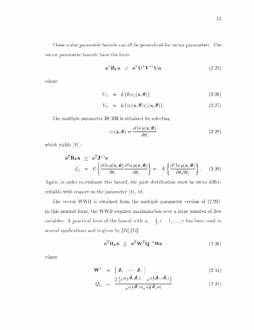
These scalar parameter bounds can all be generalized for vector parameters. The
vector parameter bounds have the form:
aTR�a � aTUTV�1Ua (2.25)
where
Uij = Ef�i j(x;�)g (2.26)
Vij = Ef i(x;�) j(x;�)g: (2.27)
The multiple parameter BCRB is obtained by selecting
i(x;�) =@ ln p(x;�)
@�i(2.28)
which yields [31]:
aTR�a � aTJ�1a
Jij = E
(@ ln p(x;�)
@�i
@ ln p(x;�)
@�j
)= �E
(@2 ln p(x;�)
@�i@�j
): (2.29)
Again, in order to evaluate this bound, the joint distribution must be twice di�er-
entiable with respect to the parameter [31, 18].
The vector WWB is obtained from the multiple parameter version of (2.20).
In this general form, the WWB requires maximization over a large number of free
variables. A practical form of the bound with si =12; i = 1; : : : ; r has been used in
several applications and is given by [22],[42]:
aTR�a � aTWTQ�1Wa (2.30)
where
WT =h�1 � � � �r
i(2.31)
Qij =2�e�(
12;�i;�j) � e�(
12;�i;��j)
�e�(
12 ;�i;0)e�(
12 ;�j;0)
(2.32)

13
and
�( 12 ; �i; �j) = lnE
8<:vuutp(x;� + �i)
p(x;�)
p(x;� + �j)
p(x;�)
9=; (2.33)
= lnZ�
qp(� + �i)p(� + �j)
�Z qp(xj� + �i)p(xj� + �j)dx
�d�:
Again, integration with respect to � is over the region � = f� : p(�) > 0g. In
implementing the bound, we must choose the test points f�igri=1. For a non-singularbound, there must be at least K linearly independent test points.
The WWB has been shown to be a useful bound for all regions of operation
[18],[39]-[43]. The only major di�culty in implementing the bound is in choosing
the test points and in inverting the matrix Q.
2.3 Summary
The WWB and ZZB are derived using di�erent techniques and no underlying the-
oretical relationship between the two bounds has been developed. They have both
been used for threshold analysis and are useful over a wide range of operating con-
ditions. Comparisons between the two bounds have been carried out through com-
putational examples, in which the WWB tends to be tighter in the very low SNR
region, while the ZZB tends to be tighter in the asymptotic region and provides a
better prediction of the threshold location [18, 43]. The WWB can be applied to
arbitrarily distributed vector parameters, but the ZZB was derived only for scalar,
uniformly distributed parameters.
In this dissertation, the ZZB is extended to arbitrarily distributed vector param-
eters. Properties of the bound are presented as well as some further variations and
extensions. The relationship between the Weiss-Weinstein family of bounds and the
extended Ziv-Zakai bound is also explored, and a new bound in the Weiss-Weinstein

14
family is proposed which can also be derived in the Ziv-Zakai formulation. In the
examples, we compute the EZZB for arbitrarily distributed vector parameters and
compare it to the WWB and BCRB. The EZZB is shown to be the tightest bound
in the threshold and asymptotic regions.

Chapter 3
Extended Ziv-Zakai Bound
In this chapter, the Bellini-Tartara form of the Ziv-Zakai bound is extended for
arbitrarily distributed vector parameters. We begin by generalizing the bound for a
scalar parameter with arbitrary prior distribution. The derivation uses the elements
of the original proofs in [15]-[17], but is presented in a more straightforward manner.
This formulation provides the framework for the derivation of several variations and
extensions to the general scalar bound. These include some bounds which are weaker
but easier to evaluate, a bound on the MSE in estimating a function of a random
variable, a tighter bound in terms of the probability of error in an M -ary detection
problem, bounds for distortion functions other than MSE, and extension of all the
above mentioned bounds to arbitrarily distributed vector parameters.
3.1 Scalar Parameter with Arbitrary Prior
Theorem 3.1 The MSE in estimating the scalar random variable � with prior pdf
p(�) is lower bounded by:
�2 �Z 1
0
�
2� V
�Z 1
�1(p(') + p(' +�)) � Pmin(';'+�)d'
�d� (3.1)
where V f�g denotes the valley-�lling function and Pmin(';' + �) is the minimum
probability of error in the binary detection problem:
H0 : � = '; Pr(H0) =p(')
p(') + p(' +�); x � p(xj� = ')
H1 : � = '+�; Pr(H1) = 1� Pr(H0); x � p(xj� = '+�):(3.2)
15

16
Proof. We start from the relation [60, p. 24]:
�2 =Z 1
0
�
2Pr�j�j � �
2
�d�: (3.3)
Since both � and Pr�j�j � �
2
�are non-negative, a lower bound on �2 can be obtained
from a lower bound on Pr�j�j � �
2
�.
Pr�j�j � �
2
�= Pr
�� >
�
2
�+ Pr
�� � ��
2
�(3.4)
=Z 1
�1p('0) Pr
�� >
�
2
���� � = '0
�d'0
+Z 1
�1p('1) Pr
�� � ��
2
���� � = '1
�d'1: (3.5)
Let '0 = ' and '1 = '+�. Expanding � = �̂(x)� � gives:
Pr�j�j � �
2
�=
Z 1
�1p(') Pr
��̂(x) > '+
�
2
���� � = '
�
+p(' +�)Pr��̂(x) � '+
�
2
���� � = '+��d' (3.6)
=Z 1
�1(p(') + p('+�)) �"
p(')
p(') + p(' +�)Pr��̂(x) > '+
�
2
���� � = '
�
+p('+�)
p(') + p(' +�)Pr��̂(x) � '+
�
2
���� � = '+��#d': (3.7)
Consider the detection problem de�ned in (3.2) and the suboptimal decision rule
in which the parameter is �rst estimated and a decision is made in favor of its
\nearest-neighbor":
Decide H0 : � = ' if �̂(x) � '+ �2
Decide H1 : � = '+� if �̂(x) > '+ �2 :
(3.8)
The term in square brackets in (3.7) is the probability of error for the suboptimal de-
cision scheme. If the suboptimal error probability is lower bounded by the minimum
probability of error for the detection problem, we have
Pr�j�j � �
2
��
Z 1
�1(p(') + p('+�)) � Pmin(';'+�)d': (3.9)

17
Now since Pr�j�j � �
2
�is a non-increasing function of �, it can be more tightly
bounded by applying the valley-�lling function to the right hand side of (3.9). This
produces a bound that is also non-increasing in �:
Pr�j�j � �
2
�� V
�Z 1
�1(p(') + p(' +�)) � Pmin(';'+�)d'
�: (3.10)
Substituting (3.10) into (3.3) gives the desired bound on MSE. 2
Remarks.
1) For generality, the regions of integration over ' and � have not been explicitly
de�ned. However, since Pmin(';'+�) is zero when one of the hypotheses has zero
probability, integration with respect to ' is restricted to the region in which both
p(') and p('+�) are non-zero, and the upper limit for integration with respect to
� is the length of the interval over which p(') is non-zero.
2) When � is uniformly distributed on [T0; T1], the bound (3.10) on Pr�j�j � �
2
�reduces to Kotelnikov's inequality (2.4), and the MSE bound is equal to the Bellini-
Tartara bound (2.7). If valley-�lling is omitted, the weaker bound of Chazan-Zakai-
Ziv [16] is obtained. Note that when the a priori pdf is uniform, the hypotheses in
the detection problem (3.2) are equally likely.
3) A bound similar to (3.1) for non-uniform discrete parameters can be found in
[58], but which is worse by a factor of two.
4) The bound (3.1) coincides with the minimum MSE, achieved by conditional
mean estimator, �̂(x) = Ef�jxg � m�jx, when the conditional density p(�jx) is
symmetric and unimodal. Under these conditions, we have:
Z 1
0
�
2� V
�Z 1
�1(p(') + p(' +�)) � Pmin(';'+�)d'
�d�
=Z 1
0
�
2� V
�Ex
�Z 1
�1min(p('jx); p('+�jx))d'
��d� (3.11)
=Z 1
0
�
2� V
(Ex
"Z m�jx+�2
�1p(' +�jx)d'+
Z 1
m�jx+�2
p('jx))d'#)
d� (3.12)

18
=Z 1
0
�
2� V
(Ex
"Z m�jx��2
�1p('jx)d'+
Z 1
m�jx+�2
p('jx)d'#)
d� (3.13)
=Z 1
0
�
2� V
�Ex
�Pr�j� �m�jxj � �
2
����x���
d� (3.14)
=Z 1
0
�
2� Ex
�Pr�j� �m�jxj � �
2
����x��d� (3.15)
= Ex
�Z 1
0
�
2Pr�jm�jx � �j � �
2
����x�d��
(3.16)
= Ex
nEh(m�jx � �)2
���xio : (3.17)
= En(m�jx � �)2
o: (3.18)
In going from (3.11) to (3.12), we have used the fact that since p(�jx) is symmetric
about m�jx and unimodal, p('jx) � p('+�jx) when ' � m�jx+�2 and p('+�jx) <
p('jx) when ' > m�jx + �2 . There is equality in (3.15) because the term inside the
brackets is non-increasing in � and valley-�lling is trivial.
5) If the a priori pdf is symmetric and unimodal, the bound (3.1) is equal to the
prior variance in the region of very low SNR and/or observation time. In this region
the observations are essentially useless, therefore
Pmin(';'+�) =min(p('); p(' +�))
p(') + p('+�)(3.19)
and the bound has the form:
Z 1
0
�
2� V
�Z 1
�1min(p('); p(' +�)) d'
�d�: (3.20)
If m� and �2� denote the prior mean and variance of �, and p(�) is symmetric about
its mean and unimodal, then by the same arguments as in (3.11)-(3.18), (3.20) is
equal to Z 1
0
�
2Pr�j� �m�j � �
2
�d� = E
n(� �m�)
2o= �2� : (3.21)

19
3.2 Equally Likely Hypothesis Bound
In the bound of Theorem 3.1, the di�cult problem of computing the MSE has
been transformed into the less di�cult problem of computing and integrating the
minimumprobability of error. However, the bound is useful only when Pmin(';'+�)
can either be calculated or tightly lower bounded. In many problems, this is easier
if the detection problem involves equally likely hypotheses. The bound (3.1) can be
modi�ed so that the detection problem has this property as follows:
Theorem 3.2
�2 �Z 1
0
�
2� V
�Z 1
�12min (p('); p(' +�)) � P el
min(';'+�)d'�d�: (3.22)
where V f�g denotes the valley-�lling function and P elmin(';' + �) is the minimum
probability of error in the binary detection problem:
H0 : � = '; Pr(H0) =12 ; x � p(xj� = ')
H1 : � = '+�; Pr(H1) =12; x � p(xj� = '+�);
(3.23)
The bound (3.22) for equally likely hypotheses equals the general bound of Theorem
3.1 when the prior pdf is uniform, otherwise it is weaker.
Proof. We follow the proof of Theorem 3.1 through (3.6), which can be lower
bounded by:
Pr�j�j � �
2
��
Z 1
�12min(p('); p(' +�)) �
�1
2Pr��̂ > '+
�
2
���� � = '
�
+1
2Pr��̂ � '+
�
2
���� � = '+���d': (3.24)
The term in square brackets is the probability of error in the suboptimal nearest-
neighbor decision scheme when the two hypotheses are equally likely. It can be lower
bounded by the minimum probability of error, P elmin(';'+�), from which (3.22) is
immediate.

20
By inspection, we see that the bound (3.22) and the bound of Theorem 3.1
coincide when the prior pdf is uniform. To show that the bound (3.22) is weaker
than the general bound in all other cases, we show that
(p(') + p(' +�))�Pmin(';'+�) � 2min (p('); p(' +�)) �P elmin(';'+�): (3.25)
Rewriting the left hand side,
(p(') + p('+�)) � Pmin(';'+�)
=Zx
min (p(')p(xj'); p('+�)p(xj'+�))dx: (3.26)
Now for any positive numbers a, b, c, and d,
min(ab; cd) � min(a; c) �min(b; d): (3.27)
Therefore
(p(') + p('+�)) � Pmin(';'+�)
�Zx
2min (p('); p(' +�)) �min�1
2p(xj'); 1
2p(xj'+�)
�dx (3.28)
= 2min (p('); p('+�)) � P elmin(';'+�):2 (3.29)
Even though the equally likely hypothesis bound in Theorem 3.2 is weaker than
the general bound in Theorem 3.1, it can be quite valuable in a practical sense. In
the examples, we consider a problem in which there is no closed form expression
for either Pmin(';'+�) or P elmin(';'+�) and lower bounds on the probability of
error must be used. In this case a tight bound for P elmin(';'+ �) is available, but
no comparable expression for Pmin(';'+�) is known. Probability of error bounds
are discussed in more detail in Chapter 5.

21
3.3 Single Test Point Bound
When a suitable expression or lower bound for the probability of error is available,
the remaining computational di�culty in implementing the bounds in Theorems
3.1 and 3.2 is in the integration over �. Weinstein [57] proposed a weaker form of
the Bellini-Tartara bound (2.8) in which the integral is replaced by a sum of terms
evaluated at a set of arbitrarily chosen \test points". This approach can also be
applied here. At one extreme, when a large number of test points are used with
valley-�lling, the sum becomes a method for numerical integration. At the other
extreme, the single test point bound (2.9) is easy to evaluate but may not provide a
close approximation to the integral. A stronger single test point bound is provided
in the following theorem.
Theorem 3.3
�2 � max�
�2
2
Z 1
�1(p(') + p('+�)) � Pmin(';'+�)d' (3.30)
where Pmin(';' + �) is the minimum probability of error in the binary detection
problem:
H0 : � = '; Pr(H0) =p(')
p(') + p(' +�); x � p(xj� = ')
H1 : � = '+�; Pr(H1) = 1� Pr(H0); x � p(xj� = '+�):(3.31)
Proof. We start in the same manner as Theorem 3.1,
�2 =Z 1
0
�
2Pr�j�j � �
2
�d� (3.32)
=Z 1
0
�
2
�Z 1
�1p('0) Pr
�� >
�
2
���� � = '0
�d'0
+Z 1
�1p('1) Pr
�� � ��
2
���� � = '1
�d'1
�d� (3.33)
22
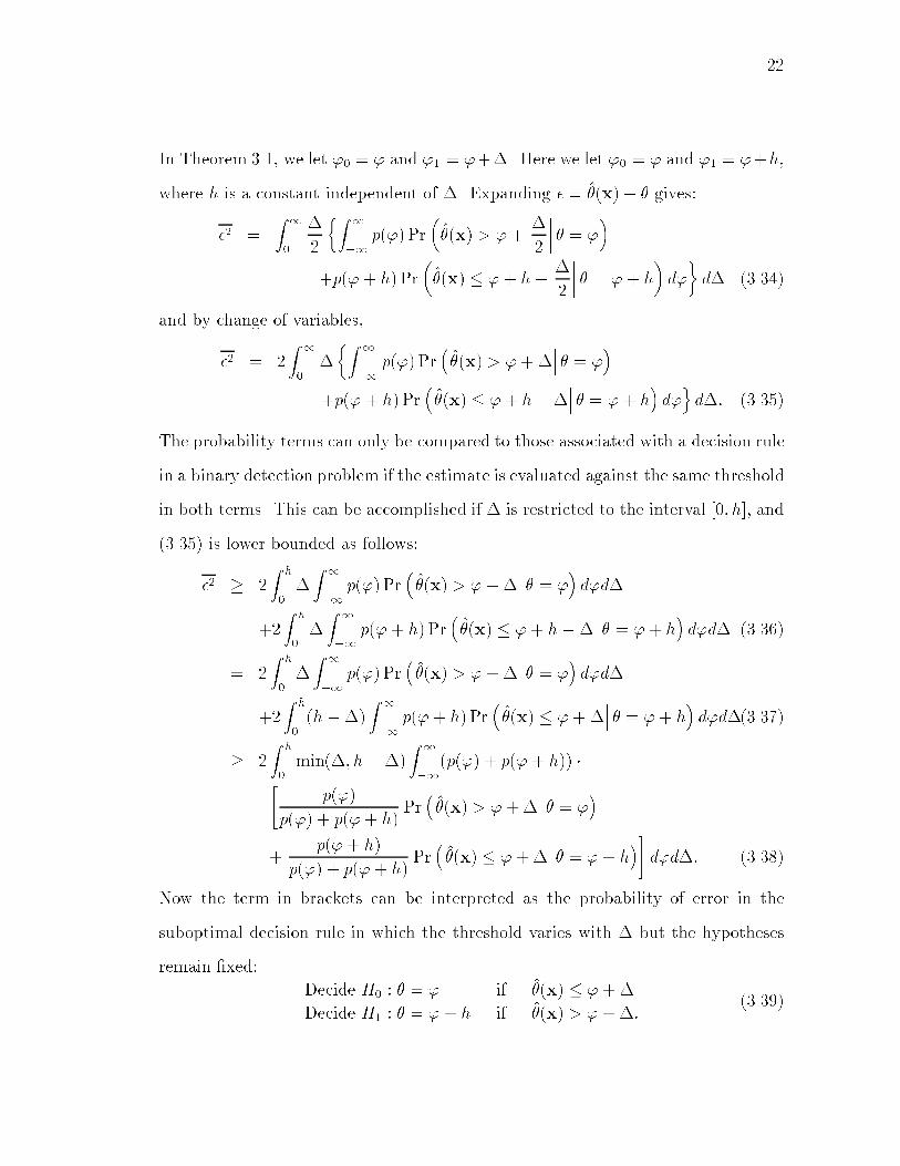
In Theorem 3.1, we let '0 = ' and '1 = '+�. Here we let '0 = ' and '1 = '+h,
where h is a constant independent of �. Expanding � = �̂(x)� � gives:
�2 =Z 1
0
�
2
�Z 1
�1p(') Pr
��̂(x) > '+
�
2
���� � = '
�
+p('+ h) Pr��̂(x) � '+ h� �
2
���� � = '+ h
�d'
�d� (3.34)
and by change of variables,
�2 = 2Z 1
0��Z 1
�1p(') Pr
��̂(x) > '+�
��� � = '�
+p(' + h) Pr��̂(x) � '+ h ��
��� � = '+ h�d'od�: (3.35)
The probability terms can only be compared to those associated with a decision rule
in a binary detection problem if the estimate is evaluated against the same threshold
in both terms. This can be accomplished if � is restricted to the interval [0; h], and
(3.35) is lower bounded as follows:
�2 � 2Z h
0�Z 1
�1p(') Pr
��̂(x) > '+�
��� � = '�d'd�
+2Z h
0�Z 1
�1p(' + h) Pr
��̂(x) � '+ h��
��� � = '+ h�d'd� (3.36)
= 2Z h
0�Z 1
�1p(') Pr
��̂(x) > '+�
��� � = '�d'd�
+2Z h
0(h��)
Z 1
�1p('+ h) Pr
��̂(x) � '+�
��� � = '+ h�d'd�(3.37)
� 2Z h
0min(�; h��)
Z 1
�1(p(') + p(' + h)) �"
p(')
p(') + p('+ h)Pr��̂(x) > '+�
��� � = '�
+p('+ h)
p(') + p('+ h)Pr��̂(x) � '+�
��� � = '+ h�#d'd�: (3.38)
Now the term in brackets can be interpreted as the probability of error in the
suboptimal decision rule in which the threshold varies with � but the hypotheses
remain �xed:
Decide H0 : � = ' if �̂(x) � '+�
Decide H1 : � = '+ h if �̂(x) > '+�:(3.39)

23
This can be lower bounded by the minimum probability of error for the detection
problem, which is independent of �:
�2 � 2Z h
0min(�; h��)d�
Z 1
�1(p(') + p(' + h)) � Pmin(';'+ h)d' (3.40)
=h2
2
Z 1
�1(p(') + p('+ h)) � Pmin(';'+ h)d': (3.41)
The bound is valid for any h and (3.30) is obtained by maximizing over h. 2
Remarks.
1) A weaker single test point bound in terms of equally likely hypotheses can be
derived as in Theorem 3.2.
2) When � is uniformly distributed on [T0; T1], the bound (3.30) becomes
�2 � max�
�2
(T1 � T0)
Z T1��
T0
P elmin(';'+�)d'; (3.42)
which is a factor of two better than Weinstein's single test point bound (2.9) and a
factor of four better than the original Ziv-Zakai bound [15].
3) It will be shown in Chapter 4 that this bound can also be derived as a member
of the Weiss-Weinstein family of bounds, thus it provides a link between the extended
Ziv-Zakai bounds and the WWB.
3.4 Bound for a Function of a Parameter
Consider estimation of a function of the parameter f(�). For any estimate f̂ (x), the
following theorem gives a bound on the mean square estimation error.
Theorem 3.4
E
��f̂(x)� f(�)
�2�
�Z 1
0
�
2� V
�Z 1
�1(p(') + p('+ g(�))) � Pmin(';'+ g(�))d'
�d� (3.43)

24
where V f�g denotes the valley-�lling function, Pmin(';' + g(�)) is the minimum
probability of error in the binary detection problem:
H0 : � = '; Pr(H0) =p(')
p(') + p('+ g(�)); x � p(xj� = ')
H1 : � = '+ g(�); Pr(H1) = 1 � Pr(H0); x � p(xj� = '+ g(�));(3.44)
and g(�) satis�es
f(' + g(�)) � f(') + � (3.45)
for every ' and �.
Proof. Proceeding as in Theorem 3.1,
E
��f̂(x)� f(�)
�2�=Z 1
0
�
2Pr�jf̂(x)� f(�)j � �
2
�d� (3.46)
and
Pr�jf̂(x)� f(�)j � �
2
�=
Z 1
�1p('0) Pr
�f̂(x) > f('0) +
�
2
���� � = '0
�d'0
+Z 1
�1p('1) Pr
�f̂(x) � f('1) ��
2
���� � = '1
�d'1: (3.47)
Letting '0 = ' and '1 = '+ g(�), where g(�) is some function of �,
Pr�jf̂(x)� f(�)j � �
2
�=Z 1
�1(p(') + p(' + g(�)))�"
p(')
p(') + p(' + g(�))Pr�f̂(x) > f(') +
�
2
���� � = '
�(3.48)
+p(' + g(�))
p(') + p(' + g(�))Pr�f̂(x) � f(' + g(�))� �
2
���� � = '+ g(�)�#d':
The term in square brackets in can be interpreted as the probability of error for a
suboptimal decision scheme in the binary detection problem de�ned in (3.44) if the
estimate f̂ (x) is compared to a common threshold, i.e. if
f(' + g(�))� �
2= f(') +
�
2: (3.49)

25
f(w)
f(W)+W
f(W+g(W))
Figure 3.1 Choosing g(�) for function of a parameter.
Furthermore, if
f('+ g(�))� �
2� f(') +
�
2; (3.50)
then the threshold on H1 is to the right of the threshold on H0, and the decision
regions overlap. In this case, the probabilities in (3.48) can be lower bounded by
shifting either or both thresholds so that they coincide. Therefore if a g(�) can be
found which satis�es (3.50) for all ' and �, then the term in brackets in (3.48) can
be lower bounded by the minimum probability of error for the detection problem.
This yields
Pr�jf̂(x)� f(�)j � �
2
��
Z 1
�1(p(') + p(' + g(�))) � Pmin(';'+ g(�))d'(3.51)
from which (3.43) follows immediately. 2
Remarks.
1) A typical f(') is shown in Figure 3.1. When the curve is shifted up � units,
g(�) is the amount the curve must be shifted horizontally to the left so that it
remains above the vertically shifted curve. If f(') is monotonically increasing in ',
g(�) is positive, and if f(') is monotonically decreasing in ', g(�) is negative.

26
2) When f(�) = k�, g(�) = �kand the bound (3.43) reduces to a scaled version
of the bound in Theorem 3.1.
3) Bounds in terms of equally likely hypotheses and single test point bounds
for a function of a parameter can be derived in a similar manner to the bounds in
Theorems 3.2 and 3.3.
3.5 M-Hypothesis Bound
The bound of Theorem 3.1 can be further generalized and improved by relating the
MSE to the probability of error in an M -ary detection problem as follows.
Theorem 3.5 For any M � 2,
�2 �Z 1
0
�
2� (3.52)
V
(1
M � 1
Z 1
�1
M�1Xn=0
p('+ n�)
!� P (M)
min (';'+�; : : : ; '+ (M � 1)�) d'
)d�
where V f�g is the valley-�lling function and P (M)min (';'+�; : : : ; '+ (M � 1)�) is
the minimum probability of error in the hypothesis testing problem with the M hy-
potheses Hi, i = 0; : : : ;M � 1:
Hi : � = '+ i�; Pr(Hi) =p(' + i�)PM�1
n=0 p(' + n�); x � p(xj� = '+ i�); (3.53)
which is illustrated in Figure 3.2. This bound coincides with the bound of Theorem
3.1 when M = 2 and is tighter when M > 2.
' '+� '+ 2� � � � '+ (M � 1)�
H0 H1 H2 � � � HM�1�̂(x)
Figure 3.2 Scalar parameter M -ary detection problem.

27
Proof. We start from (3.3) as in Theorem 3.1:
�2 =Z 1
0
�
2Pr�j�j � �
2
�d�: (3.54)
Focusing on Pr�j�j � �
2
�, we can write it as the sum of M � 1 identical terms:
Pr�j�j � �
2
�=
1
M � 1
M�1Xi=1
�Pr�� >
�
2
�+ Pr
�� � ��
2
��(3.55)
=1
M � 1
M�1Xi=1
�Z 1
�1p('i�1) Pr
�� >
�
2
���� � = 'i�1�d'i�1
+Z 1
�1p('i) Pr
�� � ��
2
���� � = 'i
�d'i
�(3.56)
=1
M � 1
M�1Xi=1
�Z 1
�1p('i�1) Pr
��̂(x) > 'i�1 +
�
2
���� � = 'i�1�d'i�1
+Z 1
�1p('i) Pr
��̂(x) � 'i � �
2
���� � = 'i
�d'i
�: (3.57)
Now let '0 = ' and 'i = '+ i� for i = 1; : : : ;M �1. Taking the summation inside
the integral gives:
Pr�j�j � �
2
�=
1
M � 1
Z 1
�1
M�1Xi=1
�p(' + (i� 1)�)Pr
��̂(x) > ' +
�i� 1
2
������ � = '+ (i� 1)�
�
+ p(' + i�)Pr��̂(x) � '+
�i� 1
2
��
���� � = '+ i���
d': (3.58)
Multiplying and dividing byPM�1
n=0 p(' + n�) and combining terms, we get:
Pr�j�j � �
2
�=
1
M � 1
Z 1
�1
M�1Xn=0
p(' + n�)
!�
24 p(')�PM�1
n=0 p(' + n�)� Pr��̂(x) > '+
�
2
���� � = '
�(3.59)
+M�2Xi=1
p(' + i�)�PM�1n=0 p(' + n�)
� �Pr��̂(x) � '+�i� 1
2
��
���� � = '+ i��
+ Pr��̂(x) > '+
�i+
1
2
������ � = '+ i�
��
+p('+ (M � 1)�)�PM�1
n=0 p('+ n�)� Pr��̂(x) � '+
�M � 1
2
������ � = '+ (M � 1)�
�35 d':

28
We can interpret the term in square brackets as the probability of error in a subop-
timal \nearest-neighbor" decision rule for the detection problem de�ned in (3.53):
Decide H0 if �̂(x) � '+ �2;
Decide Hi;i=1;:::;M�2 if '+�i� 1
2
�� < �̂(x) � '+
�i+ 1
2
��;
Decide HM�1 if �̂(x) > '+�M � 1
2
��:
(3.60)
This is illustrated in Figure 3.2. Lower bounding the suboptimal error probability
by the minimum probability of error yields:
Pr�j�j � �
2
��
1
M � 1
Z 1
�1
M�1Xn=0
p(' + n�)
!P
(M)min (';'+�; : : : ; '+ (M � 1)�) d': (3.61)
Applying valley-�lling, and substituting the result into (3.54) gives the bound (3.52).
The proof that the bound (3.52) is tighter than the binary bound of Theorem
3.1 is given in Appendix A. 2
Remarks.
1) As before, the limits on the regions of integration have been left open, however,
each integral is only evaluated over the region in which the probability of error
P(M)min (';'+�; : : : ; '+ (M � 1)�) is non-zero. Note that in regions in which one
or more, say L, of the prior densities is equal to zero, the M -ary detection problem
reduces to the corresponding (M � L)-ary detection problem.
2) A bound in terms of equally likely hypotheses can be derived similarly to
the bound in Theorem 3.2, and single test point bounds can be obtained as in
Theorem 3.3. AnM -hypothesis bound for a function of a random variable may also
be derived. It requires �nding M � 1 functions fgi(�)gMi=1 which satisfy
f('+ gi(�)) � f(' + gi�1(�)) + � (3.62)
for every ' and �, with g0(�) = 0.

29
3) Multiple hypothesis bounds were also derived in [15] and [59] for scalar, uni-
formly distributed parameters, and in [58] for non-uniform discrete parameters. In
those bounds, the number of hypotheses was determined by the size of the param-
eter space and varied with �. In the bound (3.52), M is �xed and may be chosen
arbitrarily. Furthermore, when M = 2, the bound of Theorem 3.1 is obtained. The
other multiple hypothesis bounds do not reduce to the binary hypothesis bound.
4) In generalizing to M hypotheses, the complexity of the bound increases con-
siderably since expressions or bounds on error probability for the M -ary problem
are harder to �nd. Thus, the bound may be mainly of theoretical value.
3.6 Arbitrary Distortion Measures
Estimation performance can be assessed in terms of the expected value of distor-
tion measures other than squared error. Some examples include the absolute error,
D(�) = j�j, higher moments of the error, D(�) = j�jr; r � 1, and the uniform distor-
tion measure which assigns a constant cost for all values of error with magnitude
larger than some value, i.e.,
D(�) =
(0 j�j � �
2
k j�j > �2:
(3.63)
It was noted in [16] that the Chazan-Zakai-Ziv bound could be generalized for these
distortion measures. In fact, the bounds can be extended to a larger class of dis-
tortion measures, those which are symmetric and non-decreasing, and composed of
piecewise continuously di�erentiable segments.
First consider the uniform distortion measure. Its expected value is
E fD(j�j)g = k Pr�j�j � �
2
�; (3.64)
which can be lower bounded by bounding Pr�j�j � �
2
�as was done for MSE.

30
Next consider any symmetric, non-decreasing, di�erentiable distortion measure
D(�) with D(0) = 0 and derivative _D(�). We can write the average distortion as
E fD(�)g = E fD(j�j)g =Z 1
0D(�)dPr (j�j � �) (3.65)
Integrating by parts,
E fD(�)g = D(�) Pr(j�j � �)
����10�Z 1
0
_D(�)(1� Pr (j�j � �))d�
=Z 1
0
_D(�) Pr (j�j � �)d�: (3.66)
Substituting � = 2� yields
E fD(�)g =Z 1
0
1
2_D��
2
�Pr�j�j � �
2
�d�: (3.67)
Since D(�) is non-decreasing, _D��2
�is non-negative, and we can lower bound (3.67)
by bounding Pr�j�j � �
2
�. Note that when D(�) = �2; _D(�) = 2�, and (3.67) reduces
to (3.3) as expected.
Since any symmetric, non-decreasing distortion measure composed of piecewise
continuously di�erentiable segments can be written as the sum of uniform distortion
measures and symmetric, non-decreasing, di�erentiable distortion measures, we can
lower bound the average distortion by lower bounding Pr�j�j � �
2
�, and all the
results of the previous �ve sections can be applied.
3.7 Vector Parameters with Arbitrary Prior
We now present extension to vector random parameters with arbitrary prior distri-
butions. The parameter of interest is a K-dimensional vector random variable �
with prior pdf p(�). For any estimator �̂(x), the estimation error is � = �̂(x)� �,and R� = Ef��Tg is the error correlation matrix. We are interested in lower bound-
ing aTR�a, for any K-dimensional vector a. The derivation of the vector bound is
31
based on derivation of the scalar bound of Theorem 3.1 and was jointly developed
with Steinberg and Ephraim [61, 62].
Theorem 3.6 For any K-dimensional vector a,
aTR�a �Z 1
0
�
2� V
(max
� : aT� = �
Z(p(') + p(' + �)) � Pmin(';'+ �)d'
)d�; (3.68)
where V f�g is the valley-�lling function and Pmin(';'+ �) is the minimum proba-
bility of error in the binary detection problem:
H0 : � = '; Pr(H0) =p(')
p(') + p('+ �); x � p(xj� = ')
H1 : � = '+ �; Pr(H1) = 1� Pr(H0); x � p(xj� = ' + �):(3.69)
Proof. Replacing j�j with jaT�j in (3.3) gives:
aTR�a = EnjaT�j2
o=Z 1
0
�
2Pr�jaT�j � �
2
�d�: (3.70)
Focusing on Pr�jaT�j � �
2
�, we can write:
Pr�jaT�j � �
2
�= Pr
�aT� >
�
2
�+ Pr
�aT� � ��
2
�(3.71)
=Zp('0) Pr
�aT� >
�
2
���� � = '0
�d'0
+Zp('1) Pr
�aT� � ��
2
����� = '1
�d'1 (3.72)
=Zp('0) Pr
�aT �̂(x) > aT'0 +
�
2
����� = '0
�d'0
+Zp('1) Pr
�aT �̂(x) � aT'1 �
�
2
����� = '1
�d'1: (3.73)
Let '0 = ' and '1 = '+ �. Multiplying and dividing by p(') + p('+ �) gives
Pr�jaT�j � �
2
�=Z(p(') + p('+ �))�"
p(')
p(') + p('+ �)Pr�aT �̂ > aT' +
�
2
����� = '�
+p(' + �)
p(') + p('+ �)Pr�aT �̂ � aT'+ aT� � �
2
����� = '+ ��#d': (3.74)

32
CCCCCCCCCCCCCC
CC
CC
CC
CC
CC
CC
�����������������������������������
t
t
����
����
����
�����
���:
a
t�̂
�0 = '
�1 = ' + ���H1
H0
aT� = aT'+ �2
aT� = aT'+�
Figure 3.3 Vector parameter binary detection problem.
Now consider the detection problem de�ned in (3.69). If � is chosen so that
aT� = �; (3.75)
then the term in square brackets in (3.74) represents the probability of error in the
suboptimal decision rule:
Decide H0 : � = ' if aT �̂(x) > aT'+ �2
Decide H1 : � = '+ � if aT �̂(x) � aT'+ �2 :
(3.76)
The detection problem and suboptimal decision rule are illustrated in Figure 3.3.
The decision regions are separated by the hyperplane
aT� = aT'+�
2; (3.77)
which passes through the midpoint of the line connecting ' and ' + � and is
perpendicular to the a-axis. A decision is made in favor of the hypothesis which is
on the same side of the separating hyperplane (3.77) as the estimate, �̂(x).
33
Replacing the suboptimal probability of error by the minimum probability of
error gives:
Pr�jaT�j � �
2
��Z(p(') + p(' + �)) � Pmin(';'+ �)d': (3.78)
This is valid for any � satisfying (3.75), and the tightest bound is obtained by
maximizing over � within this constraint. Applying valley-�lling, we get
Pr�jaT�j � �
2
�
� V
(max
� : aT� = �
Z(p(') + p(' + �)) � Pmin(';'+ �)d'
): (3.79)
Substituting (3.79) into (3.70) gives the desired bound. 2
Remarks.
1) To obtain the tightest bound, we must maximize over the vector �, subject to
the constraint aT� = �. The vector � is not uniquely determined by the constraint
(3.75), and the position of the second hypothesis may lie anywhere in the hyperplane
de�ned by:
aT� = aT'+�: (3.80)
This is indicated by the dashed line in Figure 3.3. In order to satisfy the constraint,
� must be composed of a �xed component along the a-axis, �kak2 a, and an arbitrary
component orthogonal to a. Thus � has the form
� =�
kak2 a+ b; (3.81)
where b is an arbitrary vector orthogonal to a, i.e.,
aTb = 0; (3.82)
and we have K � 1 degrees of freedom in choosing � via the vector b.

34
In the maximization, we want to choose � so that the two hypotheses are as indis-
tinguishable as possible by the optimum detector, and therefore produce the largest
probability of error. Choosing b = 0 results in the hypotheses being separated
by the smallest Euclidean distance. This is often a good choice, but hypotheses
separated by the smallest Euclidean distance do not necessarily have the largest
probability of error, and maximizing over � can improve the bound.
2) Multiple parameter extensions of the scalar bounds in Theorems 3.1,3.3, and
3.5 may be obtained in a straightforward manner. The vector generalization of the
bound in Theorem 3.4 for a function of a parameter becomes quite complicated
and was not pursued. Bounds for a wide class of distortion measures may also be
derived. The vector extensions take the following forms:
i. Equally likely hypotheses
aTR�a � (3.83)Z 1
0
�
2� V
(max
� : aT� = �
Z2min (p('); p('+ �)) � P el
min(';'+ �)d'
)d�:
ii. Single Test Point
aTR�a � max�
kaT�k22
Z(p(') + p(' + �)) � Pmin(';'+ �)d' (3.84)
In this bound the maximization over � subject to the constraint aT� = �,
followed by the maximization over �, have been combined.
iii. M Hypotheses
aTR�a �Z 1
0
�
2� V
8>>>><>>>>:
max�1; : : : ; �M�1 :aT�i = i ��
f(�1; : : : ; �M�1)
9>>>>=>>>>;d� (3.85)
35
where
f(�1; : : : ; �M�1) = (3.86)
1
M � 1
Z M�1Xn=0
p('+ �n)
!� P (M)
min (';'+ �1; : : : ;'+ �M�1) d'
and �0 = 0. The optimizedM -hypothesis bound is tighter than the optimized
binary bound for M > 2. The derivation is given in Appendix A.
3) If a bound on the MSE of the ith parameter is desired, then we could also
use the scalar bound (3.1) of Theorem 3.1 with the marginal pdfs p(�i) and p(xj�i)obtained by averaging out the unwanted parameters. Alternatively, we could con-
dition the scalar bound on the remaining K � 1 parameters, and take the expected
value with respect to those parameters. If we use the vector bound with b = 0, the
resulting bound is equivalent to the second alternative when valley-�lling is omit-
ted. Assume that the component of interest is �1. If we choose a = [1 0 : : : 0]T and
� = [� 0 : : : 0]T , then
aTR�a = �21
�Z 1
0
�
2
Z(p('1; '2; : : : ; 'K) + p('1 +�; '2; : : : ; 'K)) �
Pmin('1; '1 +�j'2; : : : ; 'K)d'd� (3.87)
=Z 1
0
�
2
Zp('2; : : : ; 'K) (p('1j'2; : : : ; 'K) + p('1 +�j'2; : : : ; 'K)) �
Pmin('1; '1 +�j'2; : : : ; 'K)d'd� (3.88)
=Zp('2; : : : ; 'K)
�Z 1
0
�
2
Z(p('1j'2; : : : ; 'K) + p('1 +�j'2; : : : ; 'K)) �
Pmin('1; '1 +�j'2; : : : ; 'K)d'1d��d'2 � � � d'K (3.89)
which is the expected value of the conditional scalar bound. Note that with any
other choice of b, the vector bound does not reduce to the scalar bound.
36
4) Other multiple parameter bounds such as the Weiss-Weinstein, Cram�er-Rao,
and Barankin bounds can be expressed in terms of a matrix, B, which is a lower
bound on the correlation matrix R� in the sense that for an arbitrary vector a,
aTR�a � aTBa. The extended Ziv-Zakai bound does not usually have this form,
but conveys the same information. In both cases, bounds on the MSE of the individ-
ual parameters and any linear combination of the parameters can be obtained. The
matrix form has the advantage that the bound matrix only needs to be calculated
once, while the EZZB must be recomputed for each choice of a. But if only a small
number of parameters or combinations of parameters is of interest, the advantage
of the matrix form is not signi�cant. Furthermore, while the o�-diagonal elements
of the correlation matrix may contain important information about the interdepen-
dence of the estimation errors, the same is not true of the o�-diagonal entries in the
bound matrix. They do not provide bounds on cross-correlations, nor does a zero
vs. non-zero entry in the bound imply the same property in the correlation matrix.
3.8 Summary
In this chapter, the Ziv-Zakai bound was extended to arbitrarily distributed vector
parameters. The extended bound relates the MSE to the probability of error in a
detection problem in which a decision is made between two values of the parameter.
The prior probabilities of the hypotheses are proportional to the prior pdf evalu-
ated at the two parameter values. The derivation of the bound uses the elements of
the original proofs in [15]-[17], but is organized di�erently. In the original bounds,
the derivations begin with the detection problem and evolve into the MSE, while
the derivations presented here begin with an expression for the MSE, from which
the detection problem is immediately recognized. This formulation allowed for the

37
derivation of additional bounds such as a weaker bound in terms of equally likely
hypotheses and a bound which does not require integration over �. Further gener-
alizations included a bound for functions of a parameter, a tighter bound in terms
of an M -ary detection problem, and bounds for a large class of distortion measures.

Chapter 4
Relationship of Weiss-Weinstein Bound to Extended Ziv-Zakai Bound
With the extensions presented in Chapter 3, both the EZZB and WWB are appli-
cable to arbitrarily distributed vector parameters, and they are some of the tightest
available bounds for analysis of MSE performance for all regions of operation. The
WWB and EZZB are derived using di�erent techniques and no underlying theoreti-
cal relationship between the two bounds has been developed, therefore comparisons
between the two bounds have been made only through computational examples.
The WWB tends to be tighter in the very low SNR region, while the EZZB tends to
be tighter in the asymptotic region and provides a better prediction of the thresh-
old location. Finding a relationship between the bounds at a theoretical level may
explain these tendencies and may lead to improved bounds. In this chapter, a con-
nection between the two bounds is presented. A new bound in the Weiss-Weinstein
family is derived which is equivalent to the single test point extended Ziv-Zakai
bound in Theorem 3.3.
Recall that in the Weiss-Weinstein family of bounds, for any function (x; �)
such that E f (x; �)jxg = 0, the global MSE for a single, arbitrarily distributed
random variable can be lower bounded by:
�2 � E2f� (x; �)gEf 2(x; �)g : (4.1)
Consider the function
(x; �) = min
1;p(x; � +�
p(x; �)
!�min
1;p(x; � ��
p(x; �)
!: (4.2)
38

39
It is easily veri�ed that the condition E f (x; �)jxg = 0 is satis�ed.
E f (x; �)jxg =Z 1
�1p(�jx)min
1;p(x; � +�)
p(x; �)
!d�
�Z 1
�1p(�jx)min
1;p(x; � ��)
p(x; �)
!d� (4.3)
=Z 1
�1p(�jx)min
1;p(� +�jx)p(�jx)
!d�
�Z 1
�1p(�jx)min
1;p(� ��jx)p(�jx)
!d� (4.4)
=Z 1
�1min (p(�jx); p(� +�jx)) d�
�Z 1
�1min(p(�jx); p(� ��jx)) d�: (4.5)
Letting � = � �� in the second integral,
E f (x; �)jxg =Z 1
�1min (p(�jx); p(� +�jx)) d�
�Z 1
�1min (p(� +�jx); p(�jx))d� = 0: (4.6)
Evaluating the numerator of the bound,
Ef� (x; �)g =Zx
Z 1
�1�p(x; �)min
1;p(x; � +�)
p(x; �)
!d�dx
�Zx
Z 1
�1�p(x; �)min
1;p(x; � ��)
p(x; �)
!d�dx (4.7)
=Zx
Z 1
�1�min(p(x; �); p(x; � +�)) d�dx
�Zx
Z 1
�1�min(p(x; �); p(x; � ��)) d�dx (4.8)
Letting � = � �� in the second integral,
Ef� (x; �)g =Zx
Z 1
�1�min(p(x; �); p(x; � +�)) d�dx
�Zx
Z 1
�1(�+�)min (p(x; �+�); p(x; �)) d�dx (4.9)
= ��Zx
Z 1
�1min (p(x; � +�); p(x; �)) d�dx (4.10)
= ��Z 1
�1(p(�) + p(� +�)) � Pmin(�;�+�)d�: (4.11)
40
To evaluate the denominator, we have to compute
Ef 2(x; �)g =Zx
Z 1
�1p(x; �)
(min 2
1;p(x; � +�)
p(x; �)
!+min 2
1;p(x; � ��)
p(x; �)
!
�2min
1;p(x; � +�)
p(x; �)
!min
1;p(x; � ��)
p(x; �)
!)d�dx: (4.12)
In general, this is a di�cult expression to evaluate. However, if an upper bound on
the expression can be obtained, the inequality in (4.1) will be maintained. Note that
the terms min�1; p(x;�+�)
p(x;�)
�and min
�1; p(x;���)
p(x;�)
�have values in the interval (0; 1].
For any two numbers a and b, 0 � a; b � 1,
a2 + b2 � 2ab � a+ b (4.13)
therefore
Ef 2(x; �)g �Zx
Z 1
�1p(x; �)
(min
1;p(x; � +�)
p(x; �)
!
+min
1;p(x; � ��)
p(x; �)
!)d�dx (4.14)
= 2Zx
Z 1
�1min (p(x; �); p(x; �+ �))d�dx (4.15)
= 2Z 1
�1(p(�) + p(� +�)) � Pmin(�; � +�)d�: (4.16)
Substituting (4.11) and (4.16) into (4.1) and optimizing the free parameter �
yields the bound
�2 � max�
�2
2
Z 1
�1(p(�) + p(� +�)) � Pmin(�; � +�)d� (4.17)
which is the same as the single test point EZZB derived in Theorem 3.3.
This bound makes a connection between the extended Ziv-Zakai and Weiss-
Weinstein families of bounds. In this form, the bound is weaker than the gen-
eral EZZB, but can be tighter than the WWB (see Example 4 in Chapter 6).
Theoretically, this bound can be extended for multiple test points and to vectors of

41
parameters, however, upper bounding the expression in the denominator makes this
di�cult. Further investigation of this bound may lead to a better understanding of
the EZZB and WWB, and to improved bounds.

Chapter 5
Probability of Error Bounds
A critical factor in implementing the extended Ziv-Zakai bounds derived in Chapter 3
is in evaluating the probability of error in either a binary or M -ary detection prob-
lem. The bounds are useful only if the probability of error is known or can be
tightly lower bounded. Probability of error expressions have been derived for many
problems, as well as numerous approximations and bounds which vary in complexity
and tightness (see e.g. [31], [63]-[72]).
In the important class of problems in which the observations are Gaussian,
H0 : Pr(H0) = q; p(xjH0) � N(m0;K0)H1 : Pr(H1) = 1� q; p(xjH1) � N(m1;K1);
(5.1)
the probability of error has been well studied [31, 67]. When the covariance matrices
are equal, K0 = K1 = K, the probability of error is given by [31, p. 37]:
Pmin = q �
d+d
2
!+ (1� q) �
� d+d
2
!(5.2)
where is the threshold in the optimum (log) likelihood ratio test
= lnq
1 � q; (5.3)
d is the normalized distance between the means on the two densities
d =q(m1�m0)TK�1(m0�m1); (5.4)
and
�(z) =Z 1
z
1p2�e�
t2
2 dt: (5.5)
42

43
When the hypotheses are equally likely, q = 1 � q = 12and = 0, and the
probability of error has the simple form:
P elmin = �
d
2
!: (5.6)
When the covariance matrices are unequal, evaluation of the probability of error
becomes intractable in all but a few special cases [31, 67], and we must turn to
approximations and bounds. Some important quantities which appear frequently in
both bounds and approximations are the semi-invariant moment generating function
�(s), and its �rst two derivatives with respect to s, _�(s) and ��(s). The function
�(s) is de�ned as
�(s) � lnE�es ln
p(xjH1)p(xjH0)
�
= lnZp(xjH0)
1�sp(xjH1)sdx: (5.7)
When s = 12, e�(
12) is equal to the Bhattacharyya distance [63]. For the general
Gaussian problem �(s) is given by [67]:
�(s) = �s(1� s)
2(m1 �m0)
T [sK0 + (1 � s)K1]�1 (m1�m0)
+s
2ln jK0j+ 1 � s
2ln jK1j � 1
2ln jsK0 + (1 � s)K1j: (5.8)
When the covariance matrices are equal, K0 = K1 =K, (5.8) simpli�es to:
�(s) = �s(1� s)
2(m1 �m0)
TK�1(m1 �m0): (5.9)
When the mean vectors are equal, (5.8) becomes:
�(s) =s
2ln jK0j+ 1� s
2ln jK1j � 1
2ln jsK0 + (1� s)K1j: (5.10)
A simple upper bound on the minimum probability of error in terms of �(s) is
the Cherno� bound [31, p. 123]:
Pmin � q � ef�(s�)�s� _�(s�)g (5.11)
44
where s� is the value of s for which _�(s) is equal to the threshold :
_�(s�) = = lnq
1� q: (5.12)
It is well known that the exponent in the Cherno� bound is asymptotically optimal
[73, p. 313].
A simple lower bound is the Bhattacharyya lower bound [63]:
Pmin � q(1� q)e2�(12 ) (5.13)
which gets its name from the Bhattacharyya distance. This bound does not have
the correct exponent and can be weak asymptotically.
Shannon, Gallager, and Berlekamp [64] derived the following bounds on the
individual error probabilities PF = Pr(errorjH0) and PM = Pr(errorjH1):
PF � e
n�(s�)�s� _�(s�)�ks�
p��(s�)
oQ0 (5.14)
PM � e
n�(s�)+(1�s�) _�(s�)�k(1�s�)
p��(s�)
oQ1 (5.15)
where
Q0 +Q1 ��1� 1
k2
�(5.16)
and k may be chosen arbitrarily to optimize the bound. Shannon et. al. used
k =p2. From these inequalities, we can derive a lower bound on Pmin as follows
Pmin = qPF + (1� q)PM (5.17)
� qef�(s�)�s� _�(s�)g(Q0e
n�ks�
p��(s�)
o+Q1e
n�k(1�s�)
p��(s�)
o)(5.18)
� qe
n�(s�)�s� _�(s�)�kmax(s�;1�s�)
p��(s�)
o(Q0 +Q1) (5.19)
� qe
n�(s�)�s� _�(s�)�kmax(s�;1�s�)
p��(s�)
o �1 � 1
k2
�: (5.20)
This bound is similar to the Cherno� upper bound and has the asymptotically
optimal exponent.

45
The Cherno� upper bound, the Bhattacharyya lower bound, and the Shannon-
Gallager-Berlekamp (SGB) lower bounds are applicable to a wide class of binary
detection problems. Evaluation of the bounds involves computing �(s), _�(s), and
��(s), and �nding the value s� such that _�(s�) = . In the extended Ziv-Zakai
bounds derived in Chapter 3, the threshold varies with both ' and �, and solving
for s� can be a computational burden. It is much easier to use the equally likely
hypothesis bounds, where = 0 for every ' and � and we can solve for s� just
once. In the remainder of this section, we will focus on bounds for equally likely
hypotheses. In many cases, the optimal value of s when the hypotheses are equally
likely is s� = 12 , for which the bounds become:
P elmin � 1
2e�(
12 ) (5.21)
P elmin � 1
4e2�(
12 ) (5.22)
P elmin � 1
2e�(
12 )e�
k2
p��( 12 )
�1� 1
k2
�: (5.23)
A good approximation to the probability of error was derived by Van Trees and
Collins [31, p. 125],[66],[67, p. 40]. When the hypotheses are equally likely and
s� = 12 , their expression has the form:
P elmin � ef�( 12)+ 1
8 ��(12)g�
�1
2
q�� ( 12)
�: (5.24)
In the Gaussian detection problem (5.1) in which the covariance matrices are
equal K0 = K1 = K,
�( 12) = � 18 ��(
12) = �(m1�m0)
TK�1(m1�m0); (5.25)
and (5.24) is equal to the exact expression (5.6) for the probability of error.
When the covariance matrices are not equal, (5.24) is known only to be a good
approximation in general. However, Pierce [65] and Weiss and Weinstein [38] derived

46
the expression (5.24) as a lower bound to the probability of error for some speci�c
problems in which the hypotheses were equally likely and the mean vectors were
equal. A key element in both derivations was their expression for �(s), which had
the form
�(s) = �c ln (1 + s(1� s)�) : (5.26)
An important example in which this form is obtained is the single source bearing
estimation problem considered in the examples in Chapter 6.
Pierce also derived the following upper and lower bounds for this problem:
e�(12)
2�1 +
r�
8 ���12
�� � ef�( 12)+ 18 ��(
12)g�
�1
2
q�� ( 1
2 )�� Pmin � e�(
12)
2�1 +
r18 ���12
��(5.27)
These bounds have not been shown to hold in general because (5.8) does not always
reduce to (5.26), and extension of the bounds in (5.27) to a wider class of problems
is still an open problem. Both the upper and lower bounds have the asymptotically
optimal exponent, and are quite tight, as the upper and lower bounds di�er at most
by a factor ofp�. Asymptotically, we can expect the Pierce lower bound to be
tighter than the SGB bound. The \constant" term in the Pierce bound hasq��(1
2)
in the denominator while the \constant" term in the SGB bound hasq��(12) in the
exponent.
In evaluating the extended Ziv-Zakai bounds, we need bounds for the probability
of error which are tight not only asymptotically, but for a wide range of operating
conditions. The Pierce bound is applicable to the bearing estimation problems
considered in the examples in Chapter 6. It will be demonstrated in the examples
that the choice of probability of error bound has a signi�cant impact on the �nal
MSE bound, and that using the equally likely hypothesis bound with the Pierce
bound on the probability of error yields the tightest bound on MSE.

Chapter 6
Examples
In this chapter, we demonstrate the application and properties of the extended Ziv-
Zakai bounds derived in Chapter 3 with some examples, and compare our results
with those obtained using the BCRB and the WWB. We begin with some simple
linear estimation problems involving a Gaussian parameter in Gaussian noise, for
which the optimal estimators and their performance are known. In these examples,
the EZZB is easy to calculate and is shown to be tight, i.e. it is equal to the
performance of the optimal estimator.
We then consider a series of bearing estimation problems, in which the parameter
of interest is the direction-of-arrival of a planewave signal observed by an array of
sensors. These are highly nonlinear problems for which evaluation of the exact
performance is intractable. The EZZB is straightforward to evaluate and is shown
to be tighter than the WWB and BCRB in the threshold and asymptotic regions.
6.1 Estimation of a Gaussian Parameter in Gaussian Noise
Example 1. Let
xi = � + ni; i = 1; : : : ; N (6.1)
where the ni are independent Gaussian random variables, N(0; �2n), and � is Gaussian
N(0; �2� ), independent of the ni. The a posteriori pdf p(�jx) is Gaussian, N(m�jx; �2p),
47

48
where [31, p. 59]:
m�jx =N�2�
N�2� + �2n
1
N
NXi=1
xi
!(6.2)
�2p =�2��
2n
N�2� + �2n: (6.3)
The minimum MSE estimator of � is m�jx and the minimum MSE is �2p. In this
example, p(�jx) is symmetric and unimodal, therefore the scalar bound (3.1) of
Theorem 3.1 should equal �2p. To evaluate the bound, we use (5.2) for Pmin(�; �+�)
with
q =p(�)
p(�) + p(� +�)(6.4)
=p(�)
p(� +�)(6.5)
d =
pN�
�n: (6.6)
Straightforward evaluation of (3.1) with this expression yields
�2 �Z 1
0� � �
�
2�p
!d� = �2p: (6.7)
Since p(�) is symmetric and unimodal, the bound converges to the prior variance �2�
as N ! 0 and as�2�
�2n! 0, as expected.
In this problem, we can also evaluate the M -ary bound (3.52) of Theorem 3.5.
Since theM -ary bound is always as least as good as the binary bound, it must equal
�2p. For any M � 2, Pmin(�; � +�; : : : ; � + (M � 1)�) has the form:
Pmin(�; � +�; : : : ; � + (M � 1)�) =1PM�1
n=0 p(� + n�)�
M�1Xi=1
p(� + (i� 1)�)�
ln id
+d
2
!+ p(� + i�)�
� ln i+1
d+d
2
!(6.8)
where
i =p(� + (i� 1)�)
p(� + i�): (6.9)

49
By inspection, we see that the key inequality (A.20) from Lemma 1, Appendix A,
which guarantees that the M -ary bound is at least as tight as the binary bound, is
an equality for this example. Therefore, when (6.8) is substituted into (3.52), the
expression is equal to the binary bound, �2p.
In comparison, if we evaluate the WWB with one test point and s = 12given in
(2.24), we obtain:
�2 � max�
�2e� �2
4�2p
2
1� e
� �2
2�2p
! : (6.10)
The bound is maximized for � = 0 and is equal to the minimumMSE �2p. The single
test point WWB is equal to the BCRB when � ! 0 [18], therefore the BCRB is
also equal to �2p. This can be veri�ed by direct evaluation of (2.13).
Example 2. Suppose now that the average absolute error in Example 1 is lower
bounded. The optimal estimator is the median of p(�jx) [31, p. 57] which is equal
to m�jx, and
Efj� �m�jxjg =s2
��p: (6.11)
The EZZB for this problem is
Efj�jg �Z 1
0
1
2V
�Z 1
�1(p(�) + p(� +�)) � Pmin(�; � +�)d�
�d�: (6.12)
Using the same expression for Pmin(�; � +�) as in Example 1 in (6.12) yields
�2 �Z 1
0�
�
2�p
!d� =
s2
��p: (6.13)
In fact, since p(�jx) is symmetric and unimodal, the EZZB will be tight for any
distortion measure which is symmetric, non-decreasing, composed of piecewise con-
tinuously di�erentiable segments, and satis�es
lim�!1
D(�)p(�jx) = 0: (6.14)
50
Under these conditions, the optimal estimator is m�jx [31, p. 61], and equality in
the bound can be shown similarly to (3.11)-(3.18). The WWB and BCRB are not
applicable to this problem.
Example 3. Now consider estimation of the vector parameter � from the obser-
vation vector x:
xi = � + ni; i = 1; : : : ; N (6.15)
where the ni are independent Gaussian random vectors, N(0;Kn), and � is a
Gaussian random vector, N(0;K�), independent of the ni. The a posteriori pdf
p(�jx) is multivariate Gaussian, N(m�jx;Kp), where
m�jx = NK�(NK� +Kn)�1 1
N
NXi=1
xi
!(6.16)
Kp = K�(NK� +Kn)�1Kn: (6.17)
The minimumMSE estimator is m�jx and the minimumMSE correlation matrix is
Kp. The probability of error Pmin(�;� + �) is again given by (5.2) with
q =p(�)
p(�) + p(� + �)(6.18)
=p(�)
p(� + �)(6.19)
d =qN�TK�1
n �: (6.20)
Substituting this expression in the vector bound (3.68) yields
aTR�a �Z 1
0� � V
8<: max� : aT� = �
�
0@q�TK�1
p �
2
1A9=; d�: (6.21)
The function �(�) is a decreasing function of its argument, therefore we want to
minimize �TK�1p � subject to the constraint aT� = �. The optimal � is
� =�Kpa
aTKpa(6.22)

51
and (6.21) becomes
aTR�a �Z 1
0� � �
0@ �
2qaTKpa
1A d� = aTKpa; (6.23)
which is the desired bound. In this example, the extended Ziv-Zakai bound is a
matrix bound which is valid for any a.
Evaluation of the multiple parameter BCRB (2.29) also yields the bound aTKpa.
Evaluating the the vector WWB (2.30)-(2.32) with multiple test points and then
optimizing is a tedious procedure. However, the optimum WWB is guaranteed to
be at least as tight as the BCRB [18], therefore we can conclude that the WWB is
also equal to aTKpa.
6.2 Bearing Estimation
An important class of parameter estimation problems is signal parameter estimation,
where the vector of unknown parameters � is embedded in a signal waveform s(t;�).
The noisy measurements are a sample function of a vector random process
x(t) = s(t;�) + n(t) � T
2� t � T
2(6.24)
where n(t) is the noise waveform. In the simple (i. e. single sensor) time delay
estimation problem, the signal waveform is known except for its delay, and the
measurements have the form
x(t) = s(t� � ) + n(t) � T
2� t � T
2(6.25)
Where � = � is the parameter of interest. In the array processing problem, mea-
surements are taken at several spatially separated sensors. We consider the problem
in which a planewave signal impinges on a planar array of M sensors as illustrated
in Figure 6.1. The ith sensor is located at

52
Figure 6.1 Geometry of the single source bearingestimation problem using a planar array.
di =
"dx;idy;i
#(6.26)
in the x � y plane. The bearing has two components which can be expressed in
either angular or Cartesian (wavenumber) coordinates:
� =
"�
�
#=
24 arcsin
�qu2x + u2y
�arctan
��uy
ux
�35 (6.27)
u =
"uxuy
#=
"cos � sin�� sin � sin�
#: (6.28)
The observed waveform at ith sensor consists of a delayed version of the source signal
and additive noise:
xi(t) = s(t� �i) + ni(t) � T
2� t � T
2(6.29)
where
�i =uTdi
c; (6.30)

53
and c is the speed of propagation. In this problem, the spatial characteristics of the
array allow for the estimation of the bearing under a variety of signal models.
Estimation of the source bearing is a fundamental problem in radar, sonar, mo-
bile communications, medical imaging, anti-jam communications, and seismic anal-
ysis. Many estimation schemes have been proposed and computation of bounds on
achievable performance has attracted much attention (see e.g. [36]-[56]), but the
ZZB has not been widely used due to its limitation to a single uniformly distributed
parameter. In the following examples, the extended Ziv-Zakai bounds derived in
Chapter 3 are used in a variety of bearing estimation problems.
We assume that the source and noise waveforms are sample functions of inde-
pendent, zero-mean, Gaussian random processes with known spectra. The source is
narrowband with spectrum
P (!) =
(P j! � !0j � W
2
0 otherwise(6.31)
where W
!0� 1, and the noise is white with power spectral density N0
2 . We are inter-
ested in estimation of u. Under these assumptions, the observations are Gaussian
with zero mean and covariance
K(!) = P (!)E(!;u)E(!;u)y +N0
2I (6.32)
where
E(!;u) =
2664e�j
!cuTd1
...
e�j!cuTdM
3775 : (6.33)
The detection problem is a Gaussian problem with equal mean vectors and covari-
ance matrices given by:
H0 : � = u; K0(!) = P (!)E(!;u)E(!;u)y + N02 I
H1 : � = u+ �; K1(!) = P (!)E(!;u+ �)E(!;u+ �)y + N02 I:
(6.34)

54
In this problem, neither Pmin(u;u + �) nor P elmin(u;u + �) can be written in closed
form, and one of the bounds from Chapter 5 must be used. These bounds all require
the function �(s;u;u+ �). For reasonably large time-bandwidth product, WT
2�� 1,
�(s;u;u+ �) has the following form [67, p. 67]:
�(s;u;u+ �) = T
Z 1
0s ln jK0(!)j+ (1 � s) ln jK1(!)j
� ln jsK0(!) + (1 � s)K1(!)j d!2�: (6.35)
The determinants in (6.35) are straightforward to evaluate (see e.g. [36]-[40],[42]),
jK0(!)j = jK1(!)j =
8><>:�N02
�M �1 + 2MP
N0
�j! � !0j � W
2�N02
�Motherwise
(6.36)
and
jsK0(!) + (1� s)K1(!)j
=
8><>:�N02
�M �1 + 2MP
N0+ s(1 � s)
�2MP
N0
�2(1� j�(�)j2)
�j! � !0j � W
2�N02
�Motherwise
(6.37)
where
�(�) � 1
ME(!0;u+ �)
yE(!0;u): (6.38)
Substitution of (6.36) and (6.37) into (6.35) yields
�(s; �) = �TZ !0+
W2
!0�W2
ln [1 + s(1 � s)�(�)]d!
2�(6.39)
= �WT
2�ln [1 + s(1� s)�(�)] (6.40)
where
�(�) � ��1� j�(�)j2
�(6.41)
� ��2MP
N0
�21 +
�2MP
N0
� : (6.42)
55
Note that �(s; �), and hence the probability of error bounds, are only a function
of � and not a function of u. This simpli�es the computation of both the EZZB and
WWB. The equally likely hypothesis bound of Theorem 3.2 is the most straightfor-
ward to implement, and the Pierce bound as well as the SGB and Bhattacharyya
bounds can be applied. Solving _�(s) = 0 gives s = 12and
�( 12 ; �) = �WT
2�ln�1 +
1
4�(�)
�(6.43)
_�( 12 ; �) = 0 (6.44)
��( 12; �) =
WT
2�
2�(�)
1 + 14�(�)
: (6.45)
Denoting the probability of error bound by P elb , the �nal EZZB has the form
aTR�a �Z 2
0� � V
(max
� : aT� = �P elb (�)A(�)
)d�: (6.46)
where
A(�) =Zmin(p(u); p(u + �))du: (6.47)
Evaluation of P elb (�) depends on the geometry of the array and A(�) depends on
the a priori distribution of u.
For comparison, the BCRB for this problem is:
Jij = �ZU
@2
@ui@ujln p(u)du +
WT
2�
�!0
c
�2 8�M
MXm=1
di;mdj;m
!: (6.48)
In order to evaluate the BCRB, we must be able to di�erentiate the prior distribution
twice with respect to the parameters.
The WWB is given by (2.30)-(2.32), where �( 12; �i; �j) has the form:
�( 12 ; �i; �j) = lnC(�i; �j) + �( 12 ; �i � �j) (6.49)
C(�i; �j) =ZU
qp(u + �i)p(u + �j)du; (6.50)
and the region of integration is U = fu : p(u) > 0g.
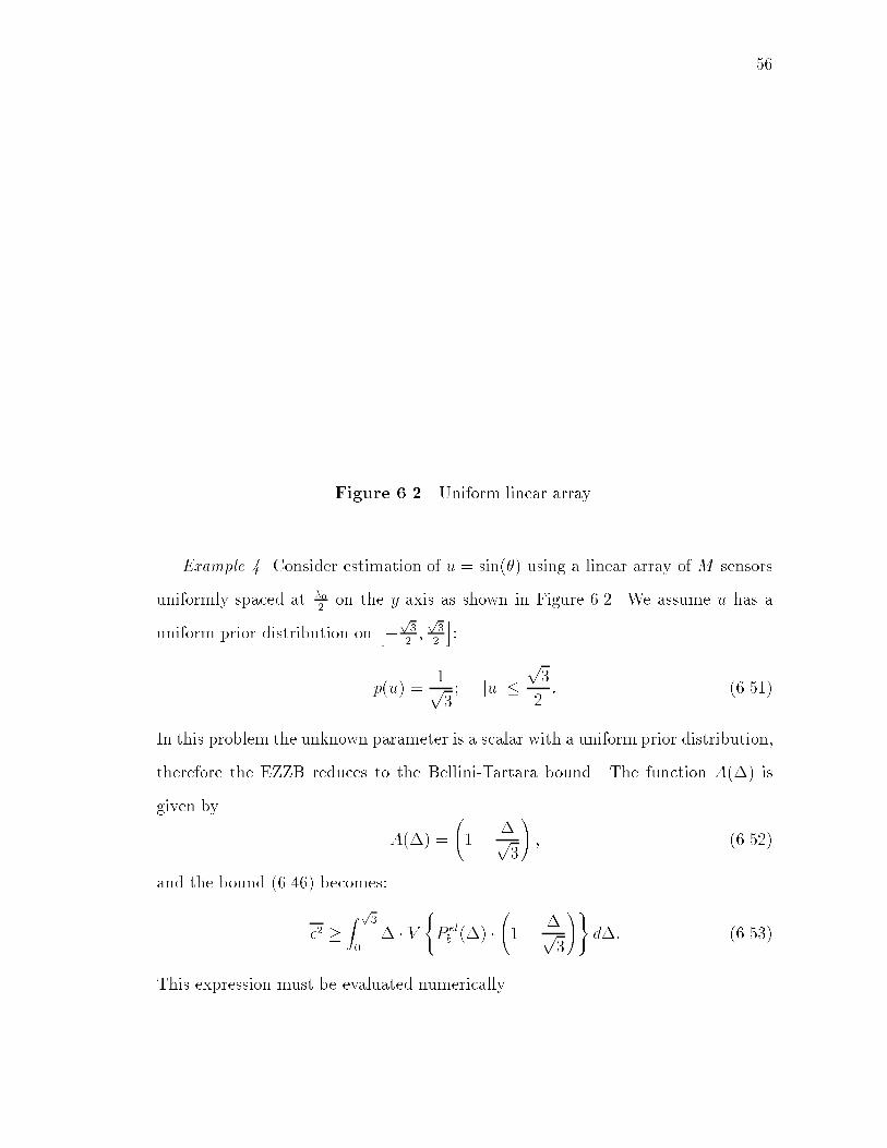
56
Figure 6.2 Uniform linear array.
Example 4. Consider estimation of u = sin(�) using a linear array of M sensors
uniformly spaced at �02on the y-axis as shown in Figure 6.2. We assume u has a
uniform prior distribution onh�
p32;p32
i:
p(u) =1p3; juj �
p3
2: (6.51)
In this problem the unknown parameter is a scalar with a uniform prior distribution,
therefore the EZZB reduces to the Bellini-Tartara bound. The function A(�) is
given by
A(�) =
1� �p
3
!; (6.52)
and the bound (6.46) becomes:
�2 �Z p
3
0� � V
(P elb (�) �
1 � �p
3
!)d�: (6.53)
This expression must be evaluated numerically.

57
The bound (6.53) was evaluated using the Pierce (5.27), Bhattacharyya (5.22),
and SGB (5.23) lower bounds, as well as the Pierce (5.27) and Cherno� (5.21) upper
bounds. The results, normalized with respect to the a priori variance, are plotted
for an 8-element array and WT
2�= 100 in Figure 6.3. First note that the curves
computed using upper bounds on the probability of error do not produce lower
bounds on MSE. They are plotted to demonstrate the sensitivity of the EZZB to
the probability of error expression. The curves computed using the Pierce upper
and lower bounds are less than 1 dB apart, therefore we can conclude that using the
Pierce lower bound in place of the actual probability of error does not signi�cantly
impact the EZZB. However, the same is not true when the SGB and Bhattacharyya
bounds are used. The SGB and Bhattacharyya bounds produce reasonable MSE
bounds which predict a threshold in performance, but they are quite a bit weaker
than the Pierce MSE bound. The Bhattacharyya curve is between 2-8 dB weaker
than the Pierce curve and the SGB curve is between 1-10 dB weaker than the Pierce
curve. The EZZB appears to be quite sensitive to the accuracy in the probability of
error expression and requires a bound on the probability of error which is tight over
a wide range of operating conditions. In the remaining examples only the Pierce
lower bound will be used.
Next, the EZZB (6.53) is compared to other bounds. The single test point (STP)
EZZB of Theorem 3.3 has the form:
�2 � max�
�2P elb (�) �
1 � �p
3
!: (6.54)
For the WWB, (6.50) reduces to:
C(�i;�j) =
1 � max(j�ij; j�jj; j�i ��jj)p
3
!: (6.55)
Evaluation of the WWB involves choosing the test points, and computing and in-
verting the matrix Q. In the WWB, adding test points always improves the bound,

58
Chernoff U.B.
Pierce U.B. & L.B.
Bhattacharyya L.B.
SGB L.B.
−30 −25 −20 −15 −10 −5−45
−40
−35
−30
−25
−20
−15
−10
−5
0
SNR (dB)
Nor
mal
ized
MS
E (
dB)
Figure 6.3 EZZB evaluated with Pierce, SGB, and Bhattacharyya lowerbounds, and Pierce and Cherno� upper bounds for 8-element linear array
and uniform distribution.

59
and we have found that if a dense set of test points is chosen, optimization of their
locations is not necessary. There is no expression for the BCRB because the uniform
prior distribution is not twice di�erentiable.
The EZZB, WWB, and STP EZZB are shown in Figure 6.4 for WT
2�= 100.
The bounds are normalized with respect to the a priori variance, and the WWB is
computed with 14 test points distributed over [0;p32]. At very low SNR, the EZZB
and WWB converge to the prior variance, but the STP EZZB converges to a value
about 0.5 dB lower. All three bounds indicate a threshold in performance, and the
WWB and EZZB converge in the asymptotic region. The STP EZZB is 2 dB lower
than the EZZB and WWB asymptotically. The WWB is tighter than both EZZBs
for low values of SNR, and the regular EZZB is tighter than the WWB and STP
EZZB in the threshold region. The STP EZZB is between 0.5 and 4 dB weaker than
the regular EZZB, but is tighter than the WWB in the threshold region. The STP
EZZB is the easiest to implement because it does not require numerical integration
or matrix inversion.
Example 5. In this example, bounds for a non-uniformly distributed scalar pa-
rameter are computed. Assume that u has a cosine squared distribution:
p(u) = cos2��
2u
�; juj � 1: (6.56)
For this problem
A(�) =
1 � �
2� sin(�2�)
�
!; (6.57)
and the bound (6.46) becomes:
�2 �Z 2
0� � V
(P elb (�) �
1� �
2� sin(�2�)
�
!)d�: (6.58)
This expression must be evaluated numerically. The STP bound is given by:
�2 � max�
�2P elb (�) �
1 � �
2� sin(�2�)
�
!: (6.59)
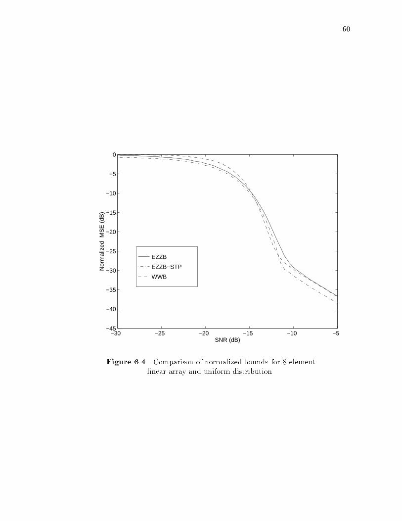
60
EZZB
EZZB−STP
WWB
−30 −25 −20 −15 −10 −5−45
−40
−35
−30
−25
−20
−15
−10
−5
0
SNR (dB)
Nor
mal
ized
MS
E (
dB)
Figure 6.4 Comparison of normalized bounds for 8-elementlinear array and uniform distribution.

61
The BCRB for this problem exists and has the form:
�2 �"�2 +
WT
2�
�2(M2 � 1)�
6
!#�1(6.60)
where � was de�ned in (6.42). It can be computed easily.
For the WWB, (6.50) reduces to:
C(�i;�j) =
1� max(�i;�j)
2
!cos
��
2j�i ��jj
�
+1
2�sin
��
2j�i ��jj
�+
1
2�sin
��
2(�i +�j)
�: (6.61)
Again, evaluation of the WWB involves choosing the test points, and computing
and inverting the matrix Q.
The four bounds are shown for an 8-element array and WT
2�= 100 in Figure 6.5.
The bounds are normalized with respect to the a priori variance, and the WWB is
computed with 14 test points distributed over [0; 1]. At very low SNR, the EZZB
and WWB converge to the prior variance, while the STP EZZB and BCRB do not
attain this value. In the asymptotic region, the EZZB, WWB, and BCRB converge,
but the STP EZZB is about 2 dB weaker. The EZZB, WWB, and STP EZZB
indicate a threshold in performance, with the WWB being tightest for low values
of SNR, and the EZZB being tightest in the threshold region. In this example the
STP EZZB is weaker than both the EZZB and WWB for all values of SNR. The
computational savings in implementing the STP EZZB are not signi�cant enough
to outweigh its weaker performance, and it will not be computed in the remaining
examples.
Example 6. In this example, estimation of the bearing angle rather than the
wavenumber is considered to demonstrate the application of the EZZB for an ar-
bitrarily distributed scalar parameter and the EZZB for a function of a parameter.
Consider the same problem as in Example 4, with the wavenumber uniformly dis-

62
EZZB
EZZB−STP
WWB
BCRB
−30 −25 −20 −15 −10 −5−45
−40
−35
−30
−25
−20
−15
−10
−5
0
SNR (dB)
Nor
mal
ized
MS
E (
dB)
Figure 6.5 Comparison of normalized bounds for 8-element lineararray and cosine squared distribution.

63
tributed onh�
p32;p32
i. The bearing angle is related to the wavenumber u by
� = arcsin(u) (6.62)
therefore � has a cosine distribution onh��
3 ;�3
i:
p(�) =1p3cos(�); j�j � �
3: (6.63)
To implement the EZZB, the equally likely hypothesis bound of Theorem 3.2 is
evaluated with the Pierce bound on the probability of error. The Pierce bound
depends on the di�erence in wavenumber, which is a function of both the di�erence
in the corresponding bearings, and the bearings themselves. The bound does not
have the same form as in wavenumber estimation (6.46), but is given by:
�2 �Z 2�
3
0� � V
(Z �3��
��3
1p3min(cos(�); cos(� +�)) �
P elb (sin(� +�)� sin(�))d�
od�:
=Z 2�
3
0� � V
(Z �3��
2
0
2p3cos
�� +
�
2
��
P elb
�sin
�� +
�
2
�� sin
�� � �
2
��d�
�d�: (6.64)
Evaluation of this bound requires numerical integration of a double integral.
Considering � to be a function of u, we can bound the MSE in estimating �
using the bound for a function of a parameter in Theorem 3.4. To evaluate (3.43),
we must �nd a function g(�) such that
arcsin(u+ g(�)) � arcsin(u) + � (6.65)
for all u 2h�
p32;p32
iand all � 2
h0; 2�
3
i. Using straightforward manipulations,
(6.65) is equivalent to
g(�) � 2 sin��
2
���u sin
��
2
�+p1 � u2 cos
��
2
��(6.66)

64
The term in brackets is never larger than 1, therefore g(�) = 2 sin��2
�satis�es
(6.65) for all u and �, and the bound is given by:
�2 �Z 2�
3
0� � V
8<:P el
b
�2 sin
��
2
���0@1 � 2 sin
��2
�p3
1A9=; d�: (6.67)
This expression must also be evaluated numerically, but there is only one integral.
The simpli�cation results from the probability of error being a function only of the
di�erence in wavenumber, which allows for direct evaluation of the integral over u.
The WWB for bearing angle estimation is most easily computed using the WWB
for a function of a parameter [18]. It has the form of (2.30):
�2 � WTQ�1W (6.68)
with
WT =h�1 � � � �r
i(6.69)
Qij =2�e�(
12 ;�i;�j) � e�(
12 ;�i;��j)
�e�(
12;�i;0)q(�i)e�(
12;�j ;0)q(�j)
(6.70)
where
q(�) =
1� 2�p
3
!arcsin
1 � 2�p
3
!� �
2+
vuut4�p3
1� �p
3
!(6.71)
and �( 12 ;�i;�j) is given by:
�( 12 ;�i;�j) = ln
1 � max(j�ij; j�jj; j�i ��jj)p
3
!+ �( 12 ;�i ��j): (6.72)
Again, evaluation of the WWB involves choosing the test points, and computing
and inverting the matrix Q.
The three bounds are shown for an 8-element array and WT
2� = 100 in Figure 6.6.
The bounds are normalized with respect to the a priori variance, and the WWB is
computed with 14 test points distributed over [0;p32 ]. At very low SNR, all three

65
EZZB
EZZB−FCN
WWB
−30 −25 −20 −15 −10 −5−40
−35
−30
−25
−20
−15
−10
−5
0
SNR (dB)
Nor
mal
ized
MS
E (
dB)
Figure 6.6 Comparison of normalized bounds for bearing estimation with8-element linear array and cosine distribution.

66
bounds converge to the prior variance, with the WWB being tighter in the low SNR
region, and EZZB being tighter in the threshold region. The EZZB for a function of
a parameter is nearly identical to the regular EZZB for low and moderate SNR and
begins to diverge in the threshold region. In the asymptotic region, the EZZB and
WWB converge, but the EZZB for a function of a parameter is about 2 dB weaker.
The regular EZZB is considerably more di�cult to compute than either the WWB
or EZZB for a function of a parameter, due to the numerical integration of a double
integral. The EZZB for a function of a parameter is simpler and yields nearly the
same bound except in the asymptotic region where it is a few dB weaker than the
other bounds.
Example 7. In the next two examples, the bounds for vector parameters are
evaluated. Estimation of the two-dimensional wavenumber using planar arrays is
considered. It is assumed that the wavenumber is uniformly distributed on the unit
disc:
p(u) =
(1�
qu2x + u2y � 1
0 otherwise.(6.73)
Under this assumption, A(�) is ��1 times the area of intersection of two unit circles
centered at the origin and �:
A(�) = 2 arccos
k�k2
!� sin
2 arccos
k�k2
!!: (6.74)
In the WWB,C(�i; �j) is ��1 the area of intersection of three unit circles centered
at the origin, �i, and �j. The formula is cumbersome and is omitted for brevity. The
uniform prior is not twice di�erentiable and there is no expression for the BCRB.
In this example, we consider a square planar array of M = 16 elements with
sensors evenly spaced �02 apart on a side, as shown in Figure 6.7. The beampattern
of the array is plotted in Figure 6.8. For this array, there are signi�cant sidelobes
along the diagonal axes. The points along these axes are points of ambiguity for the

67
t
t
t
t
t
t
t
t
t
t
t
t
t
t
t
t
�������
d = �02
x
y
Figure 6.7 Square array.
estimation problem and the detection problem, and estimation and detection errors
will tend to occur more often in these directions.
The square array is symmetric in the x and y directions, therefore the MSE in
estimating ux and uy will be the same. To evaluate the MSE in estimating ux, we
choose
a =
"10
#: (6.75)
Evaluation of the EZZB requires maximization with respect to � of the function
f(�) = P elb (�)A(�) (6.76)
which is plotted in Figure 6.9. This function is the product of the bound on prob-
ability of error for two hypotheses separated by �, and the function A(�), which is
decreasing in k�k. Because of the geometry of the array, f(�) is large not only for
small values of �, but also for the ambiguity points which lie on the axes �2 = �1 and
�2 = ��1. The maximization of f(�) with respect to � is performed for each value

68
−2−1.5
−1−0.5
00.5
11.5
2
−2
−1
0
1
2
0
0.2
0.4
0.6
0.8
1
Figure 6.8 Beampattern of 16-element square array.
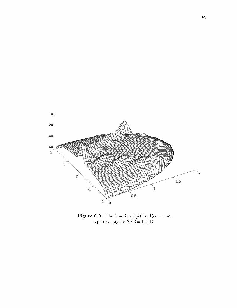
69
0
0.5
1
1.5
2
-2
-1
0
1
2-60
-40
-20
0
Figure 6.9 The function f(�) for 16-elementsquare array for SNR=-14 dB.
70
of �, subject to the constraint aT� = �. In this problem, the constraint means
that � must have the form
� =
"�b(�)
#; (6.77)
where b(�) can be chosen arbitrarily. When b = 0, f(�) is evaluated along the line
�2 = 0, but the bound can be improved by choosing b(�) so that � lies on one of the
diagonal axes. In Figure 6.10, the results of maximizing f(�) over �, valley-�lling
f(�) with b(�) = 0, and valley-�lling the maximized function are plotted. The
maximized and valley-�lled function is signi�cantly larger than the other functions,
and when it is integrated, a tighter MSE bound which captures the e�ects of the
ambiguities is produced.
The EZZB and WWB, normalized with respect to the prior variance of ux,
are plotted in Figure 6.11. Several versions of the EZZB are plotted to illustrate
the impact of valley-�lling and maximizing over �. All of the bounds approach
the prior variance for small SNR, and the WWB is tighter than the EZZB in this
region. In the threshold and high SNR regions, the use of valley-�lling alone and
maximization over � without valley-�lling produces bounds which are slightly better
than the WWB. Combining maximization with valley-�lling yields a bound which is
signi�cantly better than the other bounds in this region. In summary, the geometry
of the square array gives rise to larger estimation errors for some directions of arrival.
The EZZB re ects the presence of these large errors for high SNR, while the WWB
does not.

71
max b,VF
max b
b=0,VF
b=0
0 0.2 0.4 0.6 0.8 1 1.2 1.4 1.6 1.8 2-70
-60
-50
-40
-30
-20
-10
0
Figure 6.10 Impact of maximization and valley-�lling for16-element square array for SNR=-14 dB.
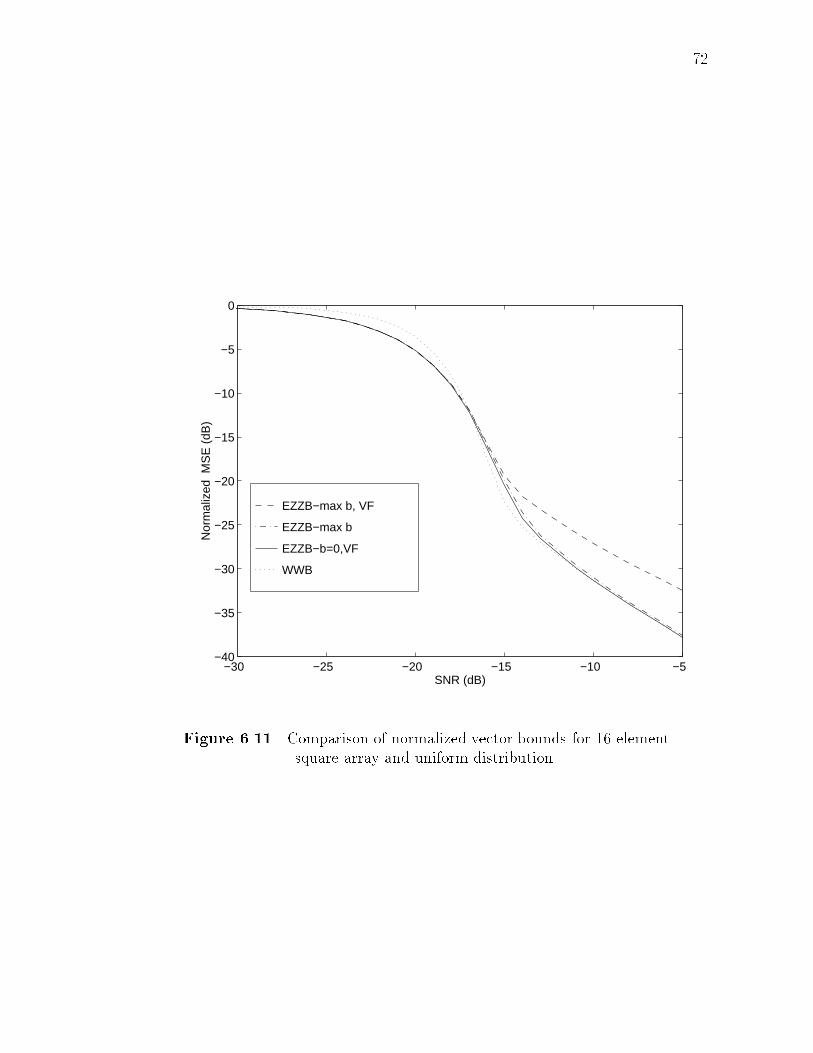
72
EZZB−max b, VF
EZZB−max b
EZZB−b=0,VF
WWB
−30 −25 −20 −15 −10 −5−40
−35
−30
−25
−20
−15
−10
−5
0
SNR (dB)
Nor
mal
ized
MS
E (
dB)
Figure 6.11 Comparison of normalized vector bounds for 16-elementsquare array and uniform distribution.

73
Example 8. Next consider the same problem as in Example 7 with a circular
planar array of M = 16 elements with sensors evenly spaced �02apart. The beam-
pattern of this array is plotted in Figure 6.12. For this array, the beampattern is
nearly the same along all axes. Since the circular array is symmetric in the x and
y directions, the MSE in estimating ux and uy will be the same, and we will again
evaluate the MSE in estimating ux. The EZZB and WWB have the same forms as in
Example 7, and only di�er in the �( 12 ; �i; �j) terms, which depend on the geometry
of the array. The function f(�) = P elb (�)A(�), plotted in Figure 6.13, is smoother
for the circular array and there are no signi�cant ambiguities as with the square
array.
The normalized EZZB and WWB are plotted vs. SNR for the circular array and
WT
2� = 100 in Figure 6.14. Once again, both the EZZB and WWB approach the
prior variance for small SNR, with the WWB being tighter than the EZZB in this
region. The EZZB is tighter in the threshold region, and both bounds converge for
high SNR. For this array, valley-�lling and maximizing over � do not improve the
bound signi�cantly.
The square and circular arrays have nearly the same performance in the low SNR
and threshold regions, but the circular array performs better than the square array
for large SNR. The square array does not possess as much symmetry as the circular
array, resulting in larger estimation errors for some directions of arrival.

74
−2−1.5
−1−0.5
00.5
11.5
2
−2
−1
0
1
2
0
0.2
0.4
0.6
0.8
1
Figure 6.12 Beampattern of 16-element circular array.

75
0
0.5
1
1.5
2
-2
-1
0
1
2-60
-40
-20
0
Figure 6.13 The function f(�) for 16-elementcircular array for SNR=-14 dB.

76
EZZB−max b, VF
EZZB−max b
EZZB−b=0,VF
WWB
−30 −25 −20 −15 −10 −5−40
−35
−30
−25
−20
−15
−10
−5
0
SNR (dB)
Nor
mal
ized
MS
E (
dB)
Figure 6.14 Comparison of normalized vector bounds for 16-elementcircular array and uniform distribution.

77
6.3 Summary
The examples in this section demonstrated the application of the extended Ziv-Zakai
bounds derived in Chapter 3. In the linear Gaussian parameter in Gaussian noise
problems, the EZZB, WWB, and BCRB were equal to the minimum MSE, and
the EZZB was also tight for other distortion measures. In the nonlinear bearing
estimation problems, the equally likely hypothesis bound was used with the Pierce
lower bound on the probability of error. In all of the examples, the EZZB was tighter
than the WWB in the threshold and asymptotic regions. When other probability
of error bounds were substituted in the EZZB, signi�cantly weaker bounds resulted,
indicating that the EZZB is quite sensitive to the accuracy of the probability of
error expression. The single test point EZZB, which was shown in Chapter 4 to
also be a member of the Weiss-Weinstein family of bounds, was computed in two
examples. It was weaker than the regular EZZB, but could be tighter than the
WWB. Although the computational savings in implementing the STP EZZB are
not signi�cant enough to outweigh its weaker performance, this bound provides a
theoretical link between the WWB and the EZZB. The EZZB for a function of a
parameter was computed for estimation of bearing angle rather than wavenumber.
It was signi�cantly easier to implement that the regular EZZB, with a small loss in
performance in the asymptotic region. Finally, the vector EZZB was computed for
estimation of two dimensional wavenumber using square and circular arrays. As in
the other examples, it was tighter in the threshold and asymptotic regions than the
WWB.

Chapter 7
Concluding Remarks
The Ziv-Zakai lower bound on the MSE in estimating a random parameter from
noisy observations has been extended to vectors of parameters with arbitrary prior
distributions. As in the original bound, the extended bound relates the MSE to
the probability of error in a binary detection problem. In the new bound, the
hypotheses in the detection problem are not required to to be equally likely, and
are related to the prior distribution of the parameter. The derivation of the bound
was made possible by developing a more concise proof of the original bound. The
new derivation allowed for the development of additional bounds such as a weaker
bound in terms of equally likely hypotheses and a single test point bound which does
not require integration. Further generalizations of the bound included a bound for
functions of a parameter, a tighter bound in terms of an M -ary detection problem,
and bounds for a large class of distortion measures.
A new bound in the Weiss-Weinstein family was presented which is equivalent
to the single test point extended Ziv-Zakai bound. This bound makes a theoretical
connection between the extended Ziv-Zakai and Weiss-Weinstein families of bounds.
Although weaker than the EZZB, it can be tighter than the WWB, and further
investigation of this bound may lead to a better understanding of the EZZB and
WWB, and to improved bounds.
The new Ziv-Zakai bounds, as well as the Weiss-Weinstein and Bayesian Cram�er-
Rao bounds, were applied to a series of bearing estimation problems, in which the
78

79
parameters of interest are the directions-of-arrival of signals received by an array of
sensors. These are highly nonlinear problems for which evaluation of the exact per-
formance is intractable. The EZZB was straightforward to evaluate and was shown
to be tighter than the WWB and BCRB in the threshold and asymptotic regions
in all of the examples. The EZZB was also analytically evaluated for some simple
linear estimation problems involving a Gaussian parameter in Gaussian noise, for
which the optimal estimators and their performance are known. In these examples,
the EZZB was shown to be tight, i.e. it is equal to the performance of the optimal
estimator.
There are several topics related to the EZZB which require further research. In
this dissertation, the EZZB was proven to equal the minimum MSE for all regions
of operation when the posterior density is symmetric and unimodal, and to equal
the prior variance for low SNR and/or observation times when the prior pdf is
symmetric and unimodal. We were not able to determine conditions under which
the bound is tight for large SNR and/or observation times, since normally this would
be done by using asymptotic properties of the probability of error. Here, however,
the hypotheses are not �xed and we need a uniformly good asymptotic bound on
the probability of error.
In previous computational comparisons between the WWB and the ZZB, as well
as in the examples considered here, the WWB tends to be tighter in the very low
SNR region, while the EZZB tends to be tighter in the asymptotic region and pro-
vides a better prediction of the threshold location. In this dissertation a theoretical
relationship between the EZZB and WWB was developed. Further exploration of
this relationship may explain these tendencies and lead to improved bounds.
The extended Ziv-Zakai bounds derived in this dissertation are useful when
the probability of error in the detection problem is known or can be tightly lower

80
bounded for a wide range of operating conditions. The Pierce lower bound used in
the bearing estimation examples is a good approximation to the probability of error
in many problems [31, 67], but is known to be a lower bound only in a few special
cases [65]-[67],[38]. Generalization of the Pierce bound to a wider class of detection
problems, or development of other tight and easily computable lower bounds on the
probability of error are open problems.
Finally, an aspect of the bounds not treated here is the formulation of the ex-
tended Ziv-Zakai bounds within the generalized rate distortion theory, as was done
by Zakai and Ziv [58]. This theory provides a general framework for generating
lower bounds by specifying a convex function and a probability measure in the Data
Processing Theorem [74]. This approach may be explored for improving the EZZB,
for �nding a relationship between the EZZB and WWB, and also for generating
tight lower bounds on the probability of error.

References
81

82
References
[1] S. Haykin, ed., Array Signal Processing, Englewood Cli�s, NJ: Prentice-Hall,Inc., 1985.
[2] B. Friedlander and B. Porat, \Performance Analysis of a Null-Steering Al-gorithm Based on Direction-of-Arrival Estimation", IEEE Trans. ASSP, vol.ASSP-37, pp. 461-466, April 1989.
[3] K. L. Bell, J. Capetanakis, and J. Bugler, \Adaptive Nulling for Multiple De-sired Signals Based on Signal Waveform Estimation", in Proceedings of IEEEMilitary Comm. Conf., (San Diego, CA), 1992.
[4] L. P. Seidman, \Performance Limitations and Error Calculations for ParameterEstimation", Proceedings of the IEEE, vol. 58, pp. 644-652, May 1970.
[5] Special Issue on Time Delay Estimation, IEEE Trans. ASSP, vol. ASSP-29,June 1981.
[6] V. A. Kotel'nikov, The Theory of Optimum Noise Immunity. New York, NY:McGraw-Hill, 1959.
[7] P. Stoica, \List of References on Spectral Line Analysis", Signal Processing,vol. 31, pp. 329-340, April 1993.
[8] R. A. Fisher, \On the Mathematical Foundations of Theoretical Statistics",Phil. Trans. Royal Soc., vol. 222, p. 309, 1922.
[9] D. Dugu�e, \Application des Proprietes de la Limite au Sens du Calcul desProbabilities a L'etude des Diverses Questions D'estimation", Ecol. Poly., vol.3, pp. 305-372, 1937.
[10] M. Fr�echet, \Sur l'extension de Certaines Evaluations Statistiques au cas dePetit Enchantillons", Rev. Inst. Int. Statist., vol. 11, pp. 182-205, 1943.
[11] G. Darmois, \Sur les Lois Limites de la Dispersion de Certaines Estimations",Rev. Inst. Int. Statist., vol. 13, pp. 9-15, 1945.
[12] C. R. Rao, \Information and Accuracy Attainable in the Estimation of Statis-tical Parameters", Bull. Calcutta Math. Soc., vol. 37, pp. 81-91, 1945.
[13] H. Cram�er, Mathematical Methods of Statistics. Princeton, NJ: Princeton Uni-versity Press, 1946.

83
[14] E. W. Barankin, \Locally Best Unbiased Estimates", Ann. Math. Stat., vol. 20,pp. 477-501, 1949.
[15] J. Ziv and M. Zakai, \Some Lower Bounds on Signal Parameter Estimation",IEEE Trans. Information Theory, vol. IT-15, pp. 386-391, May 1969.
[16] D. Chazan, M. Zakai, and J. Ziv, \Improved Lower Bounds on Signal ParameterEstimation", IEEE Trans. Information Theory, vol. IT-21, pp. 90-93, January1975.
[17] S. Bellini and G. Tartara, \Bounds on Error in Signal Parameter Estimation",IEEE Trans. Comm., vol. 22, pp. 340-342, March 1974.
[18] A. J. Weiss, Fundamental Bounds in Parameter Estimation. PhD thesis, Tel-Aviv University, Tel-Aviv, Israel, 1985.
[19] A. J. Weiss and E. Weinstein, \A Lower Bound on the Mean-Square Error inRandom Parameter Estimation", IEEE Trans. Information Theory, vol. IT-31,pp. 680-682, September 1985.
[20] E. Weinstein and A. J. Weiss, \Lower Bounds on the Mean Square EstimationError", Proceedings of the IEEE, vol. 73, pp. 1433-1434, September 1985.
[21] A. J. Weiss and E. Weinstein, \Lower Bounds in Parameter Estimation - Sum-mary of Results", in Proceedings of IEEE ICASSP, Tokyo, Japan, 1986.
[22] E. Weinstein and A. J. Weiss, \A General Class of Lower Bounds in ParameterEstimation", IEEE Trans. Information Theory, vol. 34, pp. 338-342, March1988.
[23] E. L. Lehmann, Theory of Point Estimation. New York, NY: John Wiley &Sons, 1983.
[24] I. A. Ibragimov and R. Z. Hasminskii, Statistical Estimation - Asymptotic The-ory., New York, NY: Springer-Verlag, 1981.
[25] A. Bhattacharyya, \On Some Analogues of the Amount of Information andtheir Use in Statistical Estimation", Sankhya Indian J. of Stat., vol. 8, pp.1-14, 201-218, 315-328, 1946.
[26] J. M. Hammersley, \On Estimating Restricted Parameters", J. Royal Stat. Soc.(B), vol. 12, pp. 192-240, 1950.
[27] D. G. Chapman and H. Robbins, \MinimumVariance Estimation without Reg-ularity Assumptions", Ann. Math. Stat., vol. 22, pp. 581-586, 1951.
[28] D. A. S. Fraser and I. Guttman, \Bhattacharyya Bounds without RegularityAssumptions", Ann. Math. Stat., vol. 23, pp. 629-632, 1952.

84
[29] J. Kiefer, \On Minimum Variance Estimators", Ann. Math. Stat., vol. 23, pp.627-629, 1952.
[30] J. S. Abel, \A Bound on Mean-Square-Estimate Error", IEEE Trans. Informa-tion Theory, vol. IT-39, pp. 1675-1680, September 1993.
[31] H. L. Van Trees, Detection, Estimation, and Modulation Theory, Part I. NewYork, NY: John Wiley & Sons, 1968.
[32] B. Z. Bobrovsky and M. Zakai, \A Lower Bound on the Estimation Error forCertain Di�usion Processes", IEEE Trans. Information Theory, vol. IT-22, pp.45-52, January 1976.
[33] B. Z. Bobrovsky, E. Mayer-Wolf, and M. Zakai, \Some Classes of GlobalCramer-Rao Bounds", Ann. Statistics, vol. 15, pp. 1421-1438, 1987.
[34] P. N. Misra and H. W. Sorenson, \Parameter Estimation in Poisson Processes",IEEE Trans. Information Theory, vol. IT-21, pp. 87-90, January 1975.
[35] S. C. White and N. C. Beaulieu, \On the Application of the Cramer-Rao andDetection Theory Bounds to Mean Square Error of Symbol Timing Recovery",IEEE Trans. Comm., vol. 40, pp. 1635-1643, October 1992.
[36] A. J. Weiss and E. Weinstein, \Composite Bound on the Attainable Mean-Square Error in Passive TimeDelay Estimation fromAmbiguityProne Signals",IEEE Trans. Information Theory, vol. IT-28, pp. 977-979, November 1982.
[37] A. J. Weiss and E. Weinstein, \Fundamental Limitations in Passive Time DelayEstimation - Part I: Narrow-Band Systems", IEEE Trans. ASSP, vol. ASSP-31,pp. 472-486, April 1983.
[38] E. Weinstein and A. J. Weiss, \Fundamental Limitations in Passive Time DelayEstimation - Part II: Wide-Band Systems", IEEE Trans. ASSP, vol. ASSP-32,pp. 1064-1078, October 1984.
[39] A. J. Weiss, \Composite Bound on Arrival Time Estimation Errors", IEEETrans. Aero. Elec. Syst., vol. AES-22, pp. 751-756, November 1986.
[40] A. J. Weiss, \Bounds on Time-Delay Estimation for Monochromatic Signals",IEEE Trans. Aero. Elec. Syst., vol. AES-23, pp. 798-808, November 1987.
[41] T. J. Nohara and S. Haykin, \Application of the Weiss-Weinstein Bound toa Two-Dimensional Antenna Array", IEEE Trans. ASSP, vol. ASSP-36, pp.1533-1534, September 1988.
[42] D. F. DeLong, \Use of the Weiss-Weinstein Bound to Compare the Direction-Finding Performance of Sparse Arrays", MIT Lincoln Laboratory, Lexington,MA, Tech. Rep. 982, August 1993.

85
[43] K. L. Bell, Y. Ephraim, and H. L. Van Trees, \Comparison of the Chazan-Zakai-Ziv, Weiss-Weinstein, and Cramer-Rao Bounds for Bearing Estimation",in Proceedings of Conf. on Info. Sciences and Syst., (Baltimore, MD), 1993.
[44] A. Zeira and P. M. Schultheiss, \Realizable Lower Bounds for Time DelayEstimation", IEEE Trans. Sig. Proc., vol. SP-41, pp. 3102-3113, November1993.
[45] A. B. Baggeroer, \Barankin Bounds on the Variance of Estimates of the Pa-rameters of a Gaussian Random Process", MIT Res. Lab. Electron., Quart.Prog. Rep. 92, January 1969.
[46] V. H. MacDonald and P. M. Schultheiss, \OptimumPassive Bearing Estimationin a Spatially Incoherent Environment", J. Acoust. Soc. Amer., vol. 46, pp. 37-43, July 1969.
[47] W. J. Bangs and P. M. Schultheiss, \Space-Time Processing for Optimal Pa-rameter Estimation", Proc. Signal Processing NATO Adv. Study Inst., NewYork, NY: Academic Press, 1973.
[48] S. K. Chow and P. M. Schultheiss, \Delay Estimation Using Narrow-BandProcesses", IEEE Trans. ASSP, vol. ASSP-29, pp. 478-484, June 1981.
[49] P. Stoica and A. Nehorai, \MUSIC, Maximum Likelihood and the Cramer-RaoBound", IEEE Trans. ASSP, vol. ASSP-37, pp. 720-741, May 1989.
[50] H. Clergeot, S. Tressens, and A. Ouamri, \Performance of High ResolutionFrequencies Estimation Methods Compared to the Cramer-Rao Bounds", IEEETrans. ASSP, vol. ASSP-37, pp. 1703-1720, November 1989.
[51] P. Stoica and A. Nehorai, \Performance Study of Conditional and Uncondi-tional Direction-of-Arrival Estimation", IEEE Trans. ASSP, vol. ASSP-38, pp.1783-1795, October 1990.
[52] P. Stoica and A. Nehorai, \MUSIC, Maximum Likelihood and the Cramer-RaoBound: Further Results and Comparisons", IEEE Trans. ASSP, vol. ASSP-38,pp. 2140-2150, December 1990.
[53] B. Ottersten, M. Viberg, and T. Kailath, \Analysis of Subspace Fitting and MLTechniques for Parameter Estimation from Sensor Array Data", IEEE Trans.Sig. Proc., vol. SP-40, pp. 590-599, March 1992.
[54] H. Messer, \Source Localization Performance and the Array Beampattern",Signal Processing, vol. 28, pp. 163-181, August 1992.
[55] A. Weiss and B. Friedlander, \On the Cramer-Rao Bound for Direction Findingof Correlated Signals", IEEE Trans. Sig. Proc., vol. SP-41, pp. 495-499, January1993.

86
[56] A. Zeira and P. M. Schultheiss, \Realizable Lower Bounds for Time DelayEstimation: Part II: Threshold Phenomena", IEEE Trans. Sig. Proc., vol. 42,pp. 1001-1007, May 1994.
[57] E. Weinstein, \Relations Between Belini-Tartara, Chazan-Zakai-Ziv, and Wax-Ziv Lower Bounds", IEEE Trans. Information Theory, vol. IT-34, pp. 342-343,March 1988.
[58] M. Zakai and J. Ziv, \A Generalization of the Rate-Distortion Theory andApplication", in Information Theory New Trends and Open Problems, editedby G. Longo, Springer-Verlag, 1975, pp. 87-123.
[59] L. D. Brown and R. C. Liu, \Bounds on the Bayes and Minimax Risk forSignal Parameter Estimation", IEEE Trans. Information Theory, vol. IT-39,pp. 1386-1394, July 1993.
[60] E. Cinlar, Introduction to Stochastic Processes. Englewood Cli�s, NJ: Prentice-Hall, Inc., 1975.
[61] K. L. Bell, Y. Ephraim, Y. Steinberg, and H. L. Van Trees, \Improved Bellini-Tartara Lower Bound for Parameter Estimation", in Proceedings of Intl. Symp.on Info. Theory, (Trondheim, Norway), June 1994.
[62] K. L. Bell, Y. Steinberg, Y. Ephraim, and H. L. Van Trees, \Improved Ziv-Zakai Lower Bound for Vector Parameter Estimation", in Proceedings of Info.Theory /Stat. Workshop, (Alexandria, Virginia), October 1994.
[63] T. Kailath, \The Divergence and Bhattacharyya Distance Measures in SignalSelection", IEEE Trans. Comm. Tech., vol. COM-15, pp. 52-60, February 1967.
[64] C. E. Shannon, R. G. Gallager, and E. R. Berlekamp, \Lower Bounds to ErrorProbability for Coding on Discrete Memoryless Channels. I.", Information andControl, vol. 10, pp. 65-103, February 1967.
[65] J. N. Pierce, \Approximate Error Probabilities for Optimal Diversity Combin-ing", IEEE Trans. Comm. Syst., vol. CS-11, pp. 352-354, September 1963.
[66] L. D. Collins, Asymptotic Approximation to the Error Probability for DetectingGaussian Signals. Sc.D thesis, Mass. Institute of Technology, Cambridge, MA,June 1968.
[67] H. L. Van Trees, Detection, Estimation, and Modulation Theory, Part III. NewYork, NY: John Wiley & Sons, 1971.
[68] M. Ben-Bassat and J. Raviv, \Renyi's Entropy and the Probability of Error",IEEE Trans. Information Theory, vol. IT-24, pp. 324-331, May 1978.
[69] D. E. Boekee and J. C. A. van der Lubbe, \Some Aspects of Error Bounds inFeature Selection", Pattern Recognition, vol. 11, pp. 353-360, 1979.

87
[70] D. E. Boekee and J. C. Ruitenbeek, \A Class of Lower Bounds on the BayesianProbability of Error", Information Sciences, vol. 25, pp. 21-35, 1981.
[71] M. Basseville, \Distance Measures for Signal Processing and Pattern Recogni-tion", Signal Processing, vol. 18, pp. 349-369, December 1989.
[72] M. Feder and N. Merhav, \Relations Between Entropy and Error Probability",IEEE Trans. Information Theory, vol. IT-40, pp. 259-266, January 1994.
[73] T. M. Cover and J. A. Thomas, Elements of Information Theory. New York,NY: John Wiley & Sons, 1991.
[74] J. Ziv and M. Zakai, \On Functionals Satisfying a Data-Processing Theorem",IEEE Trans. Information Theory, vol. IT-19, pp. 275-283, May 1973.

Appendices
88

Appendix A
Proof of Vector M-Hypothesis Bound
The following is a proof of the vector M -hypothesis bound given in (3.85). It
includes a proof that the vector M -hypothesis bound is tighter than the vector
binary hypothesis bound, which reduces easily to the scalar case and completes the
proof of Theorem 3.5.
Proof. We start from (3.70):
aTR�a =Z 1
0
�
2Pr�jaT�j � �
2
�d�: (A.1)
Focusing on Pr�jaT�j � �
2
�, we can write it as the sum of M � 1 identical terms:
Pr�jaT�j � �
2
�=
1
M � 1
M�1Xi=1
�Pr�aT� >
�
2
�+ Pr
�aT� � ��
2
��(A.2)
=1
M � 1
M�1Xi=1
�Zp('i�1) Pr
�aT� >
�
2
���� � = 'i�1
�d'i�1
+Zp('i) Pr
�aT� � ��
2
���� � = 'i
�d'i
�(A.3)
=1
M � 1
M�1Xi=1
�Zp('i�1) Pr
�aT �̂(x) > aT'i�1 +
�
2
����� = 'i�1
�d'i�1
+Zp('i) Pr
�aT �̂(x) � aT'i �
�
2
����� = 'i
�d'i
�: (A.4)
Now let '0 = ' and 'i = ' + �i for i = 1; : : : ;M � 1. De�ning �0 � 0 and taking
the summation inside the integral gives:
Pr�jaT�j � �
2
�=
1
M � 1
Z M�1Xi=1
�p(' + �i�1) Pr
�aT �̂(x) > aT' + aT�i�1 +
�
2
����� = ' + �i�1�
89

90
+ p('+ �i) Pr�aT �̂(x) � aT'+ aT�i � �
2
����� = ' + �i
��d': (A.5)
Multiplying and dividing byPM�1
n=0 p(' + �n) and combining terms, we get:
Pr�jaT�j � �
2
�=
1
M � 1
Z M�1Xn=0
p('+ �n)
!� (A.6)
24 p(')�PM�1
n=0 p(' + �n)� Pr�aT �̂(x) > aT' +
�
2
����� = '�
+M�2Xi=1
p('+ �i)�PM�1n=0 p(' + �n)
� �Pr�aT �̂(x) � aT'+ aT�i � �
2
����� = ' + �i
�
+ Pr�aT �̂(x) > aT'+ aT�i +
�
2
����� = '+ �i
��
+p(' + �M�1)�PM�1n=0 p(' + �n)
� Pr�aT �̂(x) � aT'+ aT�M�1 � �
2
����� = '+ �M�1�35 d':
We can interpret the term in square brackets as the probability of error in a subopti-
mal decision rule for the detection problem withM hypotheses Hi; i = 1; : : : ;M�1:
Hi : � = ' + �i; Pr(Hi) =p(' + �i)PM�1
n=0 p('+ �n); x � p(xj� = '+ �i) (A.7)
if �0 = 0 and the �i are chosen so that
aT�i = i ��; i = 1; : : : ;M � 1: (A.8)
Thus �i has the form
�i = i � �
kak2 a+ bi; (A.9)
where bi is an arbitrary vector orthogonal to a, i.e.,
aTbi = 0: (A.10)
On each of the hypotheses Hi; i = 1; : : : ;M � 1, the parameter lies on one of the
parallel hyperplanes perpendicular to the a-axis:
aT� = aT'+ i �� (A.11)

91
CCCCCCCCCCCC
CCCCCCCCCCCC
CCCCCCCCCCCC
CC
CC
CC
CC
CC
CC
CC
CC
CC
CC
CC
CC
������
������
������
������
������
� q q q
t
���:
a
t�̂
�0 = '
�1��
�2��H1
H2
H3
H0
aT� = aT'+ �2
aT� = aT'+�aT� = aT'+ 3�
2
aT� = aT'+ 2�aT� = aT'+ 5�
2
Figure A.1 Vector parameter M -ary detection problem.
This is illustrated in Figure A.1. The suboptimal decision rule makes a decision
by comparing the estimate of the parameter to the M � 1 separating hyperplanes
located midway between the hyperplanes on which the hypotheses lie, and a decision
is made is favor of the appropriate hypothesis. Formally,
Decide H0 if aT �̂(x) � aT' + �2;
Decide Hi;i=1;:::;M�2 if aT'+�i� 1
2
�� < aT �̂(x) � aT'+
�i+ 1
2
��;
Decide HM�1 if aT �̂(x) > aT'+ (M � 12)�:
(A.12)
Lower bounding the suboptimal error probability by the minimum probability of
error yields:
Pr�jaT�j � �
2
�� 1
M � 1
Z M�1Xn=0
p(' + �n)
!P
(M)min (';'+ �1; : : : ;'+ �M�1) d':
(A.13)
Maximizing over �1; : : : ; �M�1, applying valley-�lling, and substituting the result
into (A.1) gives the bound (3.85).

92
To show that the M -hypothesis bound is tighter than the binary hypothesis
bound, let B(M)(�1; : : : ; �M�1) denote the bound in (A.13), i.e.,
B(M)(�1; : : : ; �M�1) � 1
M � 1
Z M�1Xn=0
p('n)
!P
(M)min (';'+ �1; : : : ;' + �M�1) d':
(A.14)
If we let B(2)(�0) denote the optimum binary bound,
B(2)(�0) = max� : aT� = �
B(2)(�) (A.15)
and let B(M)(��1; : : : ; ��M�1) denote the optimumM -ary bound,
B(M)(��1; : : : ; ��M�1) = max
�1; : : : ; �M�1 :aT�i = i ��
B(M)(�1; : : : ; �M�1); (A.16)
then we need to show that
B(M)(��1; : : : ; ��M�1) � B(2)(�0): (A.17)
We �rst need the following Lemma.
Lemma 1. Let P (M)min
�'0; : : : ;'M�1
�denote the minimum probability of error in
the M -ary detection problem:
Hi : � = 'i; Pr(Hi) = qi; x � p(xj� = 'i); i = 0; : : : ;M � 1: (A.18)
and P(2)min
�'i;'i+1
�denote the minimumprobability of error in the binary detection
problem:
H0 : � = 'i; Pr(H0) =qi
qi + qi+1; x � p(xj� = 'i)
H1 : � = 'i+1 Pr(H1) =qi+1
qi + qi+1; x � p(xj� = 'i+1):
(A.19)
Then
P(M)min
�'0; : : : ;'M�1
��
M�2Xi=0
(qi + qi+1)P(2)min
�'i;'i+1
�: (A.20)

93
Proof.
P(M)min
�'0; : : : ;'M�1
�= 1 �
Zmax
i[qip(xj'i)] dx (A.21)
= Ex
�1 �max
i(p('ijx))
�(A.22)
= Ex
8>><>>:min
i
0BB@M�1Xn=0n 6=i
p('njx)
1CCA9>>=>>; (A.23)
Since for any M positive numbers ai; i = 0; : : : ;M � 1,
mini
M�1Xn=0n6=i
an �M�2Xi=0
min(ai; ai+1) (A.24)
we have
P(M)min
�'0; : : : ;'M�1
�� Ex
(M�2Xi=0
min�p('ijx); p('i+1jx)
�)(A.25)
=M�2Xi=0
(qi + qi+1)
1 �
Zmax
qi
qi + qi+1p(xj'i);
qi+1
qi + qi+1p(xj'i+1)
!dx
!(A.26)
=M�2Xi=0
(qi + qi+1)P(2)min
�'i;'i+1
�; (A.27)
and we have proven (A.20).
We will now show that B(M)(��1; : : : ; ��M�1) � B(2)(�0). Starting from B(2)(�0),
B(2)(�0) =Z(p(') + p('+ �0)P (2)
min (';'+ �0) d': (A.28)
Expanding into M � 1 identical terms,
B(2)(�0) =1
M � 1
M�2Xi=0
Z(p(') + p(' + �0)P (2)
min (';'+ �0) d': (A.29)
Now make the substitution ' = '+i�0, and take the summation inside the integral,
B(2)(�0) (A.30)
=1
M � 1
Z M�2Xi=0
(p(' + i�0) + p(' + (i+ 1)�0)P (2)min ('+ i�0;'+ (i+ 1)� 0) d':

94
From Lemma 1,
B(2)(�0)
� 1
M � 1
Z M�1Xn=0
p(' + n�0)
!P
(M)min (';'+ �0; : : : ;'+ (M � 1)�0) d' (A.31)
= B(M)(�0; 2�0; : : : ; (M � 1)�0) (A.32)
� B(M)(��1; : : : ; ��M�1): (A.33)
This completes the proof.

Vita
Kristine LaCroix Bell was born on August 16, 1963 in Northampton, Massachusetts,and is an American citizen. She received a Bachelor of Science degree in ElectricalEngineering fromRice University in 1985, and a Master of Science degree in ElectricalEngineering from George Mason University in 1990. From 1985 to 1990, Ms. Bellwas employed M/A-COM Linkabit and Science Applications International Corp.where she was involved in the development and analysis of military satellite com-munications systems. Since 1990, she has been a Research Instructor in the Centerof Excellence in C3I at George Mason University.
95
![Time-Spaceruzzo/papers/bag-iandc.pdfer b ounds, Barnes et al. [5 ] for an upp er b ound.) In con trast, undir e cte d graphs can b e tra v ersed in p olynomial time and logarithmic](https://img.pdfslide.us/doc/110x75/606ddde7b7341c75c97b4657/time-space-ruzzopapersbag-iandcpdf-er-b-ounds-barnes-et-al-5-for-an-upp.jpg)