II. The distributional footprint of monetary policy

39BIS Annual Economic Report 2021

II. The distributional footprint of monetary policy

The distribution of income and wealth, or economic opportunities more broadly, has gained prominence in policy debates over the past decades. Heightened awareness of these issues owes in large part to a broad-based increase in economic inequality, a trend that the uneven impact of the Covid-19 recession has exacerbated.

The growing focus on rising inequality in the central banking community, however, is more recent and dates back to the Great Financial Crisis (GFC). In its aftermath, central banks have deployed policies featuring exceptionally low interest rates and extensive use of balance sheets to support economic activity and lower unemployment. Such measures have fuelled concerns that central banks’ actions, by boosting asset prices, have benefited mostly the rich, shining the spotlight on the distributional footprint of monetary policy.

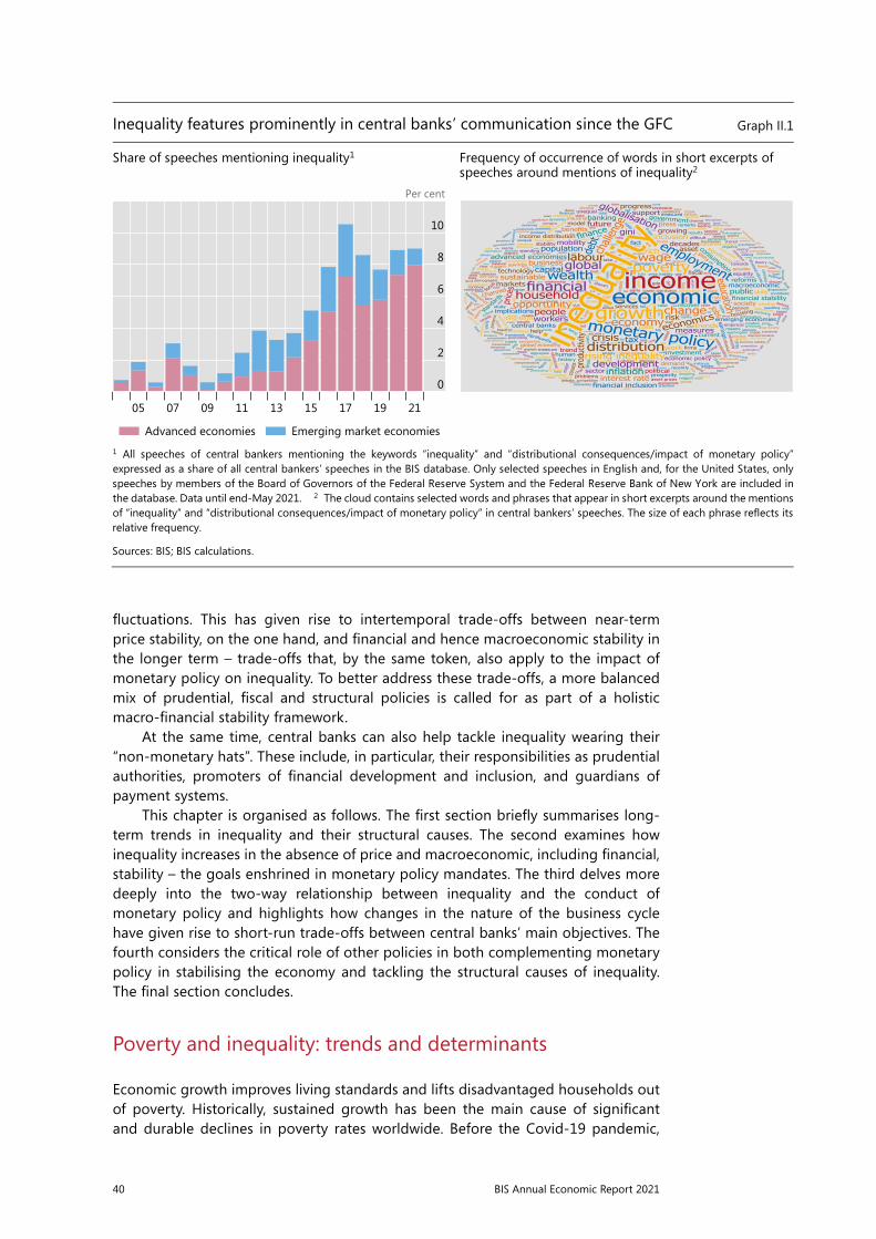
Central bankers’ greater attention to inequality concerns is reflected in the growing references to “inequality” in their public speeches (Graph II.1, left-hand panel). An analysis of the context in which inequality is mentioned suggests that central banks acknowledge the challenges posed by rising income and wealth inequality and stress the relevance of policies, including their own, in addressing distributional considerations (right-hand panel).

This chapter reviews the relation between economic inequality and the formulation and conduct of monetary policy. The trends of rising inequality since the 1980s are due to structural factors, well outside the reach of monetary policy. That said, inequality influences the transmission mechanism of monetary policy and, in turn, is affected by monetary policy over shorter time spans. The two main causes of inequality at business cycle frequency are high inflation and recessions, which disproportionately hurt the disadvantaged in society. Addressing these factors is precisely what central bank mandates call for. Therefore, the most effective way monetary policy can contribute to a more equitable society is to pursue its mandated objectives. This means keeping inflation low and limiting the incidence and duration of macroeconomic and financial instability. This task, however, has become increasingly complex over time due to a change in the nature of the business cycle: with inflation low and stable, as well as less responsive to economic slack, financial factors have come to play a bigger role in amplifying business cycle

Key takeaways

• The long-term rise in economic inequality since the 1980s is largely due to structural factors, well outside the reach of monetary policy, and is best addressed by fiscal and structural policies.

• Monetary policy can most effectively contribute to a more equitable society by fulfilling its mandate, which addresses two key factors causing inequality at shorter horizons. This requires keeping inflation low and limiting the incidence and duration of macroeconomic and financial instability, which disproportionately hurt the poor.

• Central banks can also help mitigate economic inequality wearing their “non-monetary hats”, notably as prudential authorities, promoters of financial development and inclusion, and guardians of payment systems.

40 BIS Annual Economic Report 2021

fluctuations. This has given rise to intertemporal trade-offs between near-term price stability, on the one hand, and financial and hence macroeconomic stability in the longer term – trade-offs that, by the same token, also apply to the impact of monetary policy on inequality. To better address these trade-offs, a more balanced mix of prudential, fiscal and structural policies is called for as part of a holistic macro-financial stability framework.

At the same time, central banks can also help tackle inequality wearing their “non-monetary hats”. These include, in particular, their responsibilities as prudential authorities, promoters of financial development and inclusion, and guardians of payment systems.

This chapter is organised as follows. The first section briefly summarises long-term trends in inequality and their structural causes. The second examines how inequality increases in the absence of price and macroeconomic, including financial, stability – the goals enshrined in monetary policy mandates. The third delves more deeply into the two-way relationship between inequality and the conduct of monetary policy and highlights how changes in the nature of the business cycle have given rise to short-run trade-offs between central banks’ main objectives. The fourth considers the critical role of other policies in both complementing monetary policy in stabilising the economy and tackling the structural causes of inequality. The final section concludes.

Poverty and inequality: trends and determinants

Economic growth improves living standards and lifts disadvantaged households out of poverty. Historically, sustained growth has been the main cause of significant and durable declines in poverty rates worldwide. Before the Covid-19 pandemic,

Restricted

Chapter: xx

AUTHOR/assistant: XXX/YYY/zzz

Stage: xx

FileName: Chapter_2_graph_changes_UMB.docx

Page/No of pp:

1/11

Save date and time: 16/06/2021 14:56:00

BIS XX Annual Report 1

Inequality features prominently in central banks’ communication since the GFC Graph II.1

Share of speeches mentioning inequality1 Frequency of occurrence of words in short excerpts of speeches around mentions of inequality2

Per cent

1 All speeches of central bankers mentioning the keywords “inequality” and “distributional consequences/impact of monetary policy”expressed as a share of all central bankers’ speeches in the BIS database. Only selected speeches in English and, for the United States, only speeches by members of the Board of Governors of the Federal Reserve System and the Federal Reserve Bank of New York are included in the database. Data until end-May 2021. 2 The cloud contains selected words and phrases that appear in short excerpts around the mentionsof “inequality” and “distributional consequences/impact of monetary policy” in central bankers’ speeches. The size of each phrase reflects its relative frequency.

Sources: BIS; BIS calculations.

10

8

6

4

2

0

211917151311090705

Advanced economies Emerging market economies


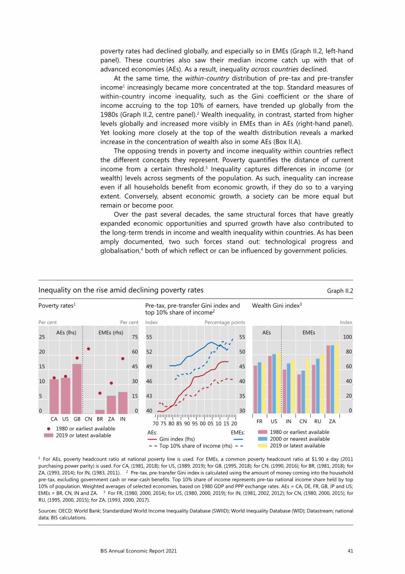
poverty rates had declined globally, and especially so in EMEs (Graph II.2, left-hand panel). These countries also saw their median income catch up with that of advanced economies (AEs). As a result, inequality across countries declined.

At the same time, the within-country distribution of pre-tax and pre-transfer income1 increasingly became more concentrated at the top. Standard measures of within-country income inequality, such as the Gini coefficient or the share of income accruing to the top 10% of earners, have trended up globally from the 1980s (Graph II.2, centre panel).2 Wealth inequality, in contrast, started from higher levels globally and increased more visibly in EMEs than in AEs (right-hand panel). Yet looking more closely at the top of the wealth distribution reveals a marked increase in the concentration of wealth also in some AEs (Box II.A).

The opposing trends in poverty and income inequality within countries reflect the different concepts they represent. Poverty quantifies the distance of current income from a certain threshold.3 Inequality captures differences in income (or wealth) levels across segments of the population. As such, inequality can increase even if all households benefit from economic growth, if they do so to a varying extent. Conversely, absent economic growth, a society can be more equal but remain or become poor.

Over the past several decades, the same structural forces that have greatly expanded economic opportunities and spurred growth have also contributed to the long-term trends in income and wealth inequality within countries. As has been amply documented, two such forces stand out: technological progress and globalisation,4 both of which reflect or can be influenced by government policies.

Restricted

Chapter: xx

AUTHOR/secretary: XXX/YYY/zzz

Stage: xx


Page/No of pp:

2/11


2 BIS XX Annual Report

Inequality on the rise amid declining poverty rates Graph II.2

Poverty rates1 Pre-tax, pre-transfer Gini index and top 10% share of income2

Wealth Gini index3

Per cent Per cent Index Percentage points Index

1 For AEs, poverty headcount ratio at national poverty line is used. For EMEs, a common poverty headcount ratio at $1.90 a day (2011 purchasing power parity) is used. For CA, (1981, 2018); for US, (1989, 2019); for GB, (1995, 2018); for CN, (1990, 2016); for BR, (1981, 2018); for ZA, (1993, 2014); for IN, (1983, 2011). 2 Pre-tax, pre-transfer Gini index is calculated using the amount of money coming into the householdpre-tax, excluding government cash or near-cash benefits. Top 10% share of income represents pre-tax national income share held by top 10% of population. Weighted averages of selected economies, based on 1980 GDP and PPP exchange rates. AEs = CA, DE, FR, GB, JP and US; EMEs = BR, CN, IN and ZA. 3 For FR, (1980, 2000, 2014); for US, (1980, 2000, 2019); for IN, (1981, 2002, 2012); for CN, (1980, 2000, 2015); forRU, (1995, 2000, 2015); for ZA, (1993, 2000, 2017).

Sources: OECD; World Bank; Standardized World Income Inequality Database (SWIID); World Inequality Database (WID); Datastream; national data; BIS calculations.

25

20

15

10

5

0

75

60

45

30

15

0INZABRCNGBUSCA

AEs (lhs) EMEs (rhs)

1980 or earliest available2019 or latest available

55

52

49

46

43

40

55

50

45

40

35

30

2015100500959085807570

Gini index (lhs)Top 10% share of income (rhs)

AEs:

EMEs:

100

80

60

40

20

0

ZARUCNINUSFR

AEs EMEs

1980 or earliest available2000 or nearest available2019 or latest available


Box II.AA taxonomy of inequality

The concept of economic inequality relates to a distribution of valuable “resources” (eg income, wealth or more generally opportunities) within a given population. As such, inequality is inherently a relative concept and is not synonymous with welfare. Nevertheless, economic inequality has important implications for social cohesion and has been studied for centuries.

By far the most widely studied forms of economic inequality concern income and wealth. Wealth inequality arises from cumulative income flows and from valuation effects on the existing stock of wealth. This complicates the comparison of income and wealth inequality. Conceptually, measures of wealth should include the (discounted) value of future income from human and financial wealth. Financial wealth is relatively easily measured through the price of assets traded on markets, although there is inevitable arbitrariness when valuing non-liquid assets such as housing or non-traded equities (eg ownership of small and medium-sized enterprises). Measuring human wealth is even more challenging, as there are no obvious proxies for the discounted present value of income from labour. For this reason, measures of wealth inequality generally omit human wealth altogether – as is also the case in this chapter. Income inequality, by contrast, is generally easier to measure, as data on income flows are routinely collected by tax authorities and surveys.

Measuring inequality typically involves summarising the heterogeneity in the distribution of the variable of interest in a single number. Popular approaches involve looking at the share of income or wealth accruing to different percentiles of the population, eg the top 10% or 1%, as well as taking ratios of top and bottom percentiles, eg the top 20% over the bottom 20%. Other measures instead seek to be more comprehensive and summarise the entire distribution by means of indices, such as the one bearing the name of Italian statistician Corrado Gini.

Different measures may yield different results, depending on which part of the distribution they focus on. By construction, looking at specific percentiles ignores what happens in the rest of the distribution. Ratios of quantiles are invariant to changes in both the numerator and the denominator, eg when an increase in the wealth accruing to the top 20% is accompanied by an increase in the bottom 20%, at the expense of the middle of the distribution. Similarly, with synthetic measures, such as the Gini coefficient, changes in different segments of the population may even out.

Restricted

Chapter: xx


Stage: xx


Page/No of pp:

9/11



Boxes

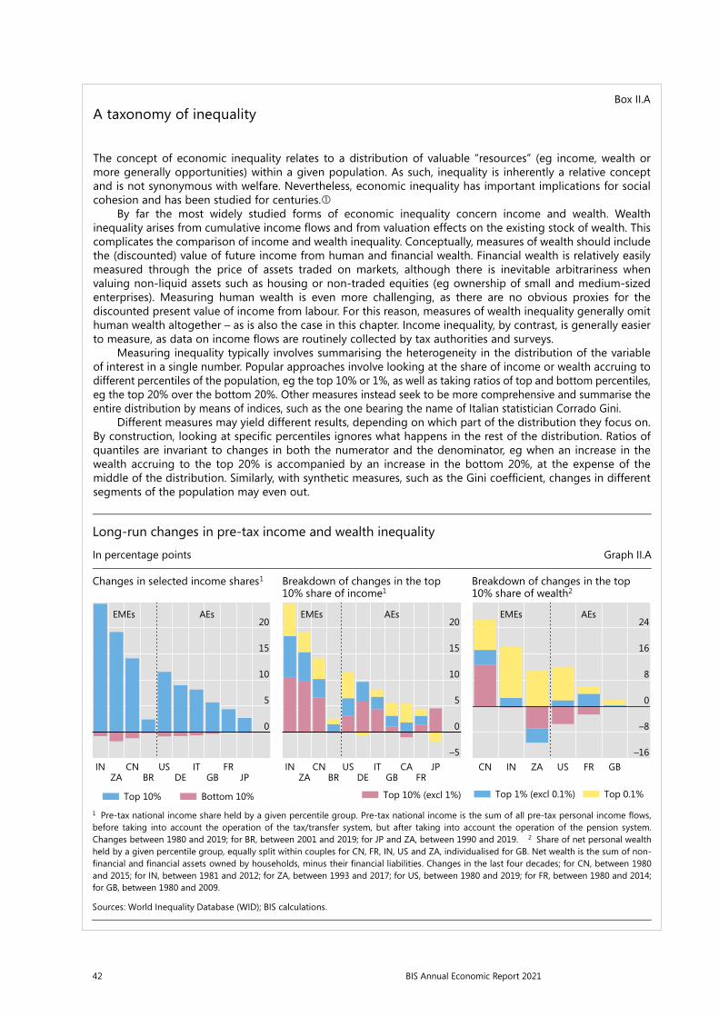
Long-run changes in pre-tax income and wealth inequality

In percentage points Graph II.A

Changes in selected income shares1 Breakdown of changes in the top 10% share of income1

Breakdown of changes in the top 10% share of wealth2

1 Pre-tax national income share held by a given percentile group. Pre-tax national income is the sum of all pre-tax personal income flows, before taking into account the operation of the tax/transfer system, but after taking into account the operation of the pension system. Changes between 1980 and 2019; for BR, between 2001 and 2019; for JP and ZA, between 1990 and 2019. 2 Share of net personal wealthheld by a given percentile group, equally split within couples for CN, FR, IN, US and ZA, individualised for GB. Net wealth is the sum of non-financial and financial assets owned by households, minus their financial liabilities. Changes in the last four decades; for CN, between 1980 and 2015; for IN, between 1981 and 2012; for ZA, between 1993 and 2017; for US, between 1980 and 2019; for FR, between 1980 and 2014;for GB, between 1980 and 2009.

Sources: World Inequality Database (WID); BIS calculations.

20

15

10

5

0

JPGBDEBRZAFRITUSCNIN

EMEs AEs

Top 10% Bottom 10%

20

15

10

5

0

–5

FRGBDEBRZAJPCAITUSCNIN

EMEs AEs

Top 10% (excl 1%)

24

16

8

0

–8

–16GBFRUSZAINCN

EMEs AEs

Top 1% (excl 0.1%) Top 0.1%


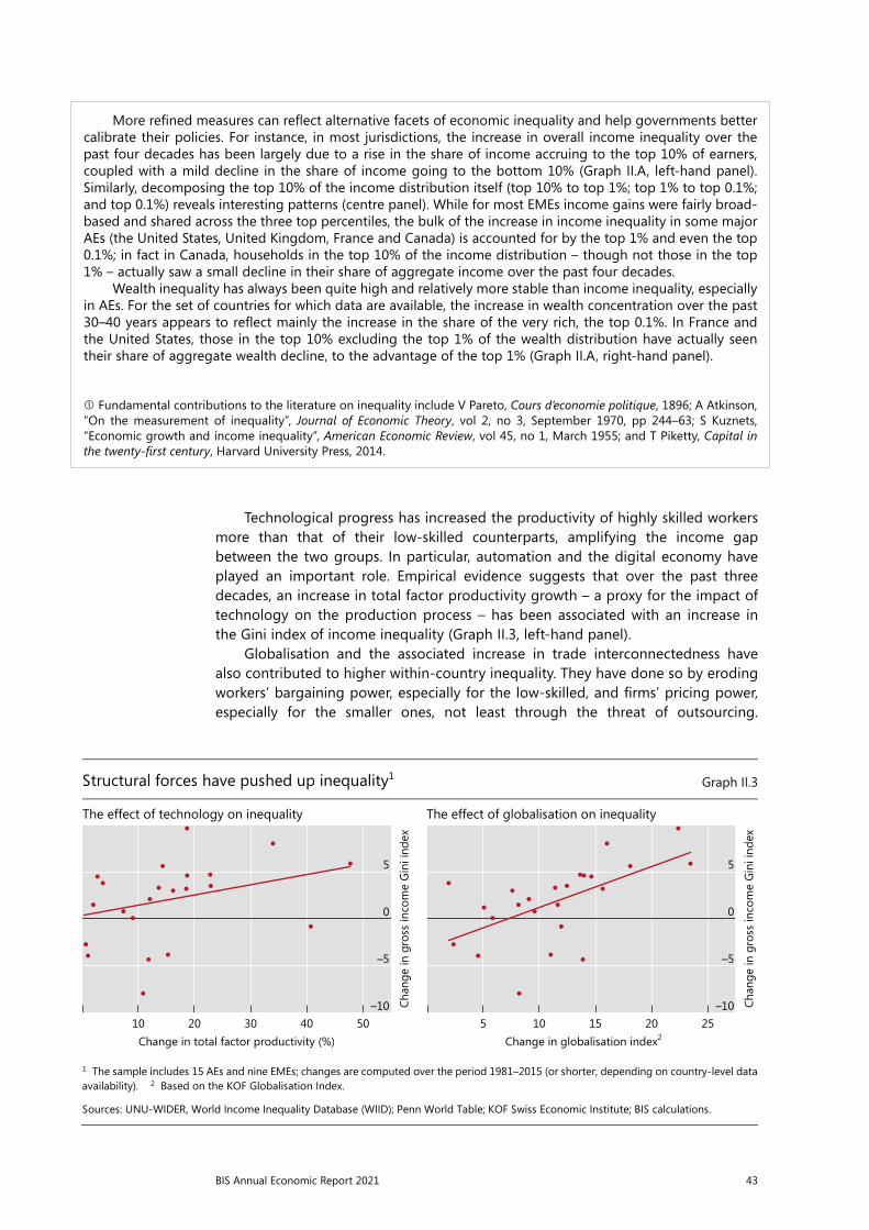
Technological progress has increased the productivity of highly skilled workers more than that of their low-skilled counterparts, amplifying the income gap between the two groups. In particular, automation and the digital economy have played an important role. Empirical evidence suggests that over the past three decades, an increase in total factor productivity growth – a proxy for the impact of technology on the production process – has been associated with an increase in the Gini index of income inequality (Graph II.3, left-hand panel).

Globalisation and the associated increase in trade interconnectedness have also contributed to higher within-country inequality. They have done so by eroding workers’ bargaining power, especially for the low-skilled, and firms’ pricing power, especially for the smaller ones, not least through the threat of outsourcing.

More refined measures can reflect alternative facets of economic inequality and help governments better calibrate their policies. For instance, in most jurisdictions, the increase in overall income inequality over the past four decades has been largely due to a rise in the share of income accruing to the top 10% of earners, coupled with a mild decline in the share of income going to the bottom 10% (Graph II.A, left-hand panel). Similarly, decomposing the top 10% of the income distribution itself (top 10% to top 1%; top 1% to top 0.1%; and top 0.1%) reveals interesting patterns (centre panel). While for most EMEs income gains were fairly broad-based and shared across the three top percentiles, the bulk of the increase in income inequality in some major AEs (the United States, United Kingdom, France and Canada) is accounted for by the top 1% and even the top 0.1%; in fact in Canada, households in the top 10% of the income distribution – though not those in the top 1% – actually saw a small decline in their share of aggregate income over the past four decades.

Wealth inequality has always been quite high and relatively more stable than income inequality, especially in AEs. For the set of countries for which data are available, the increase in wealth concentration over the past 30–40 years appears to reflect mainly the increase in the share of the very rich, the top 0.1%. In France and the United States, those in the top 10% excluding the top 1% of the wealth distribution have actually seen their share of aggregate wealth decline, to the advantage of the top 1% (Graph II.A, right-hand panel).

Fundamental contributions to the literature on inequality include V Pareto, Cours d’economie politique, 1896; A Atkinson, “On the measurement of inequality”, Journal of Economic Theory, vol 2, no 3, September 1970, pp 244–63; S Kuznets, “Economic growth and income inequality”, American Economic Review, vol 45, no 1, March 1955; and T Piketty, Capital in the twenty-first century, Harvard University Press, 2014.

Restricted

Chapter: xx


Stage: xx

FileName: Chapter_2_Graph_MfU.docx

Page/No of pp:

3/14



Structural forces have pushed up inequality1 Graph II.3

The effect of technology on inequality The effect of globalisation on inequality

1 The sample includes 15 AEs and nine EMEs; changes are computed over the period 1981–2015 (or shorter, depending on country-level data availability). 2 Based on the KOF Globalisation Index.

Sources: UNU-WIDER, World Income Inequality Database (WIID); Penn World Table; KOF Swiss Economic Institute; BIS calculations.

5

0

–5

–105040302010

Change in total factor productivity (%)

Chan

ge in

gro

ss in

com

e G

ini i

ndex

5

0

–5

–10252015105

Change in globalisation index2

Chan

ge in

gro

ss in

com

e G

ini i

ndex


Particularly in AEs, delocalisation-induced job losses in the manufacturing sectors have probably pushed lower-skilled workers towards lower value-added jobs, often in the service sectors. Empirical evidence confirms the link: globalisation goes hand in hand with rising within-country income inequality (Graph II.3, right-hand panel).

Globalisation and technological progress have naturally reinforced each other.5 Together, they have also given rise to the emergence of large “winner takes all” industries in some sectors, thereby further increasing profits and the income share of capital at the expense of that of labour.6

That said, the ultimate impact of these forces on pre-tax inequality is policy-dependent (see below).7 The benefits and opportunities that technological progress and globalisation bring could be shared more equally with the help of adequate education and training. For example, technological progress and globalisation boost the demand for highly skilled workers and polarise income distribution by increasing skill premia. Hence policies that raise the supply of skilled workers can mitigate the impact on inequality.8

Covid-19 has further exacerbated inequality due to its uneven impact and is likely to have left a significant longer-term imprint given its specific nature. The pandemic has disproportionately hit the services sector, which employs more low-skilled and low-income workers (see also Chapter I). Moreover, it has given further impetus to e-commerce and technological adoption more broadly, including in working arrangements. These demand-induced effects may be lasting ones, resulting in an impact that goes way beyond that of a standard recession.

Inequality and monetary policy mandates

Long-term structural factors such as globalisation and technology shape the environment in which monetary policy operates, but are clearly outside its influence. That said, monetary policy plays a key role in shaping other determinants of inequality at shorter horizons. Two forms of macroeconomic instability – falling squarely within monetary policy mandates9 – are especially important in this context, as they disproportionately penalise the weaker segments of the population. One is high and volatile inflation, which has been particularly important in many EMEs and is frequently coupled with meagre growth. The other is recessions, particularly when accompanied by financial instability and crises, which increase their depth and duration.10 How do these two forces, over which monetary policy has a substantial influence, affect inequality more specifically? Consider each in turn.

Inequality and inflation

In most AEs and in several EMEs, inflation has been low and stable over the past several decades. Yet it would be imprudent to forget the costs of high and runaway inflation. It is well understood that uncontrolled inflation leads to a significant misallocation of resources and numerous inefficiencies and hence to overall lower economic growth.11 While high and runaway inflation, such as that experienced by many AEs in the 1970s, can hamper growth, hyperinflation of the likes of Germany in the 1920s or Latin America in the 1980s can wreak economic havoc and in the process destroy public trust in governments and institutions.

The impact of inflation on inequality has been widely studied. Inflation shifts income and wealth away from those who are least aware of it, or least able to protect against it. These segments of the population often coincide with lower-income groups, which explains why inflation has often been portrayed as a most


regressive form of tax. The “inflation tax” takes its toll through the erosion of the value of financial assets and contracts fixed in nominal terms.

As regards wealth distribution, the financial assets that are most vulnerable to inflation are cash and bank accounts – the typical savings vehicles held by the poorest segments of the population. This is mostly because the poorest have access only to limited investment options to protect their savings. By contrast, not only can richer households avail themselves of more sophisticated inflation hedges; they may also be able to easily transfer their assets abroad, thus shielding their wealth from depreciations of the domestic currency.

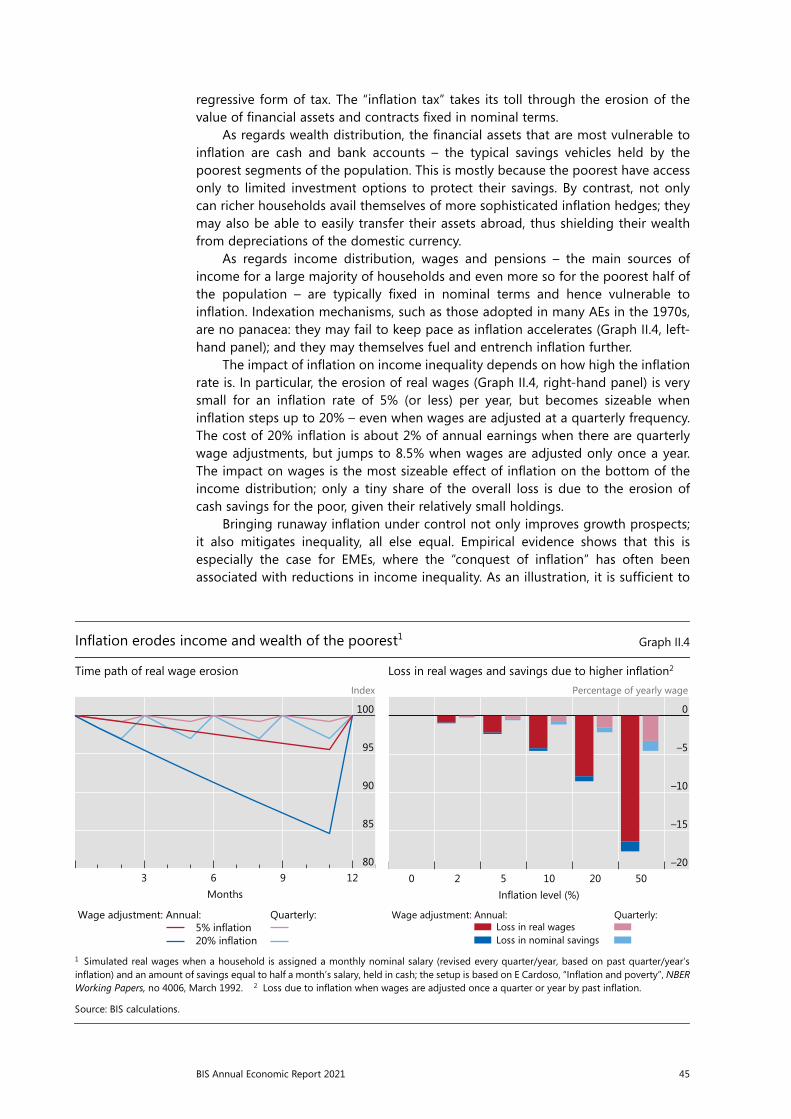
As regards income distribution, wages and pensions – the main sources of income for a large majority of households and even more so for the poorest half of the population – are typically fixed in nominal terms and hence vulnerable to inflation. Indexation mechanisms, such as those adopted in many AEs in the 1970s, are no panacea: they may fail to keep pace as inflation accelerates (Graph II.4, left-hand panel); and they may themselves fuel and entrench inflation further.

The impact of inflation on income inequality depends on how high the inflation rate is. In particular, the erosion of real wages (Graph II.4, right-hand panel) is very small for an inflation rate of 5% (or less) per year, but becomes sizeable when inflation steps up to 20% – even when wages are adjusted at a quarterly frequency. The cost of 20% inflation is about 2% of annual earnings when there are quarterly wage adjustments, but jumps to 8.5% when wages are adjusted only once a year. The impact on wages is the most sizeable effect of inflation on the bottom of the income distribution; only a tiny share of the overall loss is due to the erosion of cash savings for the poor, given their relatively small holdings.

Bringing runaway inflation under control not only improves growth prospects; it also mitigates inequality, all else equal. Empirical evidence shows that this is especially the case for EMEs, where the “conquest of inflation” has often been associated with reductions in income inequality. As an illustration, it is sufficient to

Restricted

Chapter: xx


Stage: xx


Page/No of pp:

3/11



Inflation erodes income and wealth of the poorest1 Graph II.4

Time path of real wage erosion Loss in real wages and savings due to higher inflation2

Index Percentage of yearly wage

1 Simulated real wages when a household is assigned a monthly nominal salary (revised every quarter/year, based on past quarter/year’s inflation) and an amount of savings equal to half a month’s salary, held in cash; the setup is based on E Cardoso, “Inflation and poverty”, NBERWorking Papers, no 4006, March 1992. 2 Loss due to inflation when wages are adjusted once a quarter or year by past inflation.

Source: BIS calculations.

100

95

90

85

8012963

5% inflation 20% inflation

Wage adjustment: Annual:

Quarterly:

Months

0

–5

–10

–15

–20502010520

Loss in real wagesLoss in nominal savings

Wage adjustment: Annual:

Quarterly:

Inflation level (%)


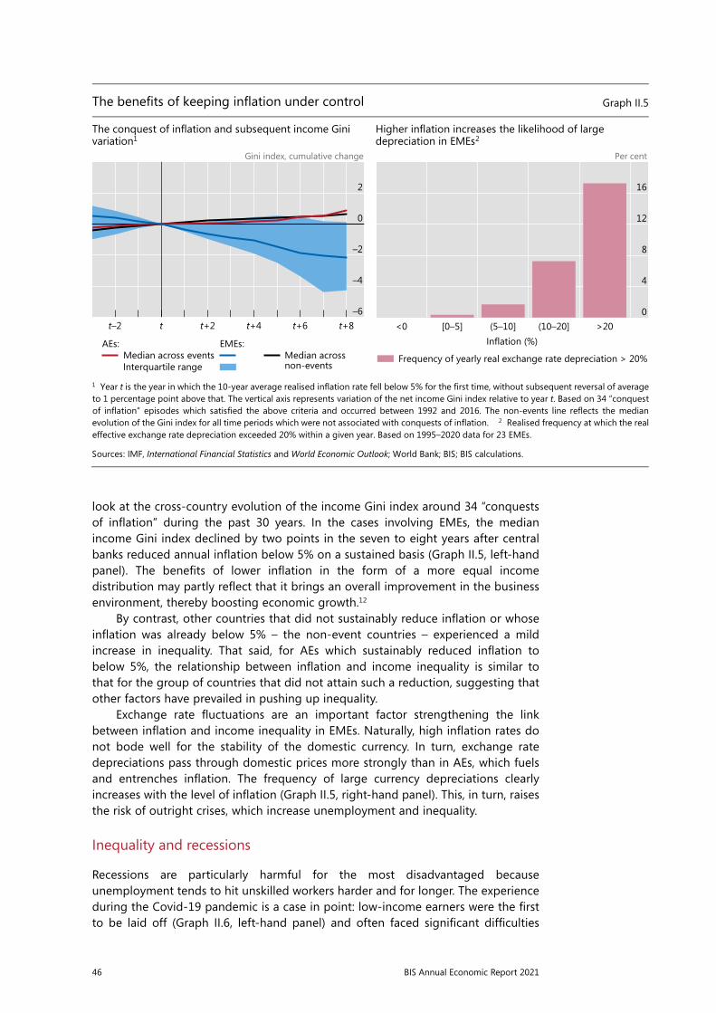
look at the cross-country evolution of the income Gini index around 34 “conquests of inflation” during the past 30 years. In the cases involving EMEs, the median income Gini index declined by two points in the seven to eight years after central banks reduced annual inflation below 5% on a sustained basis (Graph II.5, left-hand panel). The benefits of lower inflation in the form of a more equal income distribution may partly reflect that it brings an overall improvement in the business environment, thereby boosting economic growth.12

By contrast, other countries that did not sustainably reduce inflation or whose inflation was already below 5% – the non-event countries – experienced a mild increase in inequality. That said, for AEs which sustainably reduced inflation to below 5%, the relationship between inflation and income inequality is similar to that for the group of countries that did not attain such a reduction, suggesting that other factors have prevailed in pushing up inequality.

Exchange rate fluctuations are an important factor strengthening the link between inflation and income inequality in EMEs. Naturally, high inflation rates do not bode well for the stability of the domestic currency. In turn, exchange rate depreciations pass through domestic prices more strongly than in AEs, which fuels and entrenches inflation. The frequency of large currency depreciations clearly increases with the level of inflation (Graph II.5, right-hand panel). This, in turn, raises the risk of outright crises, which increase unemployment and inequality.

Inequality and recessions

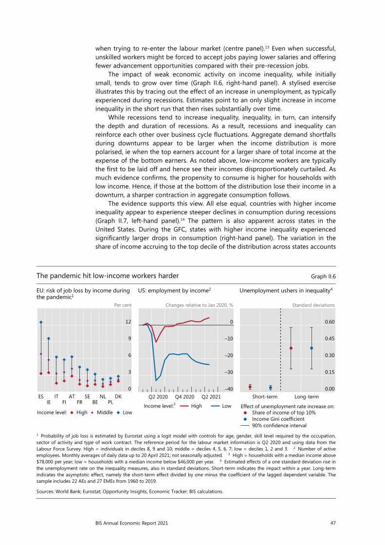
Recessions are particularly harmful for the most disadvantaged because unemployment tends to hit unskilled workers harder and for longer. The experience during the Covid-19 pandemic is a case in point: low-income earners were the first to be laid off (Graph II.6, left-hand panel) and often faced significant difficulties

Restricted

Chapter: xx


Stage: xx


Page/No of pp:

4/11



The benefits of keeping inflation under control Graph II.5

The conquest of inflation and subsequent income Gini variation1

Higher inflation increases the likelihood of large depreciation in EMEs2

Gini index, cumulative change Per cent

1 Year t is the year in which the 10-year average realised inflation rate fell below 5% for the first time, without subsequent reversal of averageto 1 percentage point above that. The vertical axis represents variation of the net income Gini index relative to year t. Based on 34 “conquest of inflation” episodes which satisfied the above criteria and occurred between 1992 and 2016. The non-events line reflects the median evolution of the Gini index for all time periods which were not associated with conquests of inflation. 2 Realised frequency at which the real effective exchange rate depreciation exceeded 20% within a given year. Based on 1995–2020 data for 23 EMEs.

Sources: IMF, International Financial Statistics and World Economic Outlook; World Bank; BIS; BIS calculations.

2

0

–2

–4

–6t–2 t t+2 t+4 t+6 t+8

Interquartile rangeMedian across events

AEs:

EMEs:

non-eventsMedian across

16

12

8

4

0>20(10–20](5–10][0–5]<0

Frequency of yearly real exchange rate depreciation > 20%

Inflation (%)


when trying to re-enter the labour market (centre panel).13 Even when successful, unskilled workers might be forced to accept jobs paying lower salaries and offering fewer advancement opportunities compared with their pre-recession jobs.

The impact of weak economic activity on income inequality, while initially small, tends to grow over time (Graph II.6, right-hand panel). A stylised exercise illustrates this by tracing out the effect of an increase in unemployment, as typically experienced during recessions. Estimates point to an only slight increase in income inequality in the short run that then rises substantially over time.

While recessions tend to increase inequality, inequality, in turn, can intensify the depth and duration of recessions. As a result, recessions and inequality can reinforce each other over business cycle fluctuations. Aggregate demand shortfalls during downturns appear to be larger when the income distribution is more polarised, ie when the top earners account for a larger share of total income at the expense of the bottom earners. As noted above, low-income workers are typically the first to be laid off and hence see their incomes disproportionately curtailed. As much evidence confirms, the propensity to consume is higher for households with low income. Hence, if those at the bottom of the distribution lose their income in a downturn, a sharper contraction in aggregate consumption follows.

The evidence supports this view. All else equal, countries with higher income inequality appear to experience steeper declines in consumption during recessions (Graph II.7, left-hand panel).14 The pattern is also apparent across states in the United States. During the GFC, states with higher income inequality experienced significantly larger drops in consumption (right-hand panel). The variation in the share of income accruing to the top decile of the distribution across states accounts

Restricted

Chapter: xx


Stage: xx


Page/No of pp:

5/11



The pandemic hit low-income workers harder Graph II.6

EU: risk of job loss by income during the pandemic1

US: employment by income2 Unemployment ushers in inequality4

Per cent Changes relative to Jan 2020, % Standard deviations

1 Probability of job loss is estimated by Eurostat using a logit model with controls for age, gender, skill level required by the occupation,sector of activity and type of work contract. The reference period for the labour market information is Q2 2020 and using data from the Labour Force Survey. High = individuals in deciles 8, 9 and 10; middle = deciles 4, 5, 6, 7; low = deciles 1, 2 and 3. 2 Number of active employees. Monthly averages of daily data up to 20 April 2021; not seasonally adjusted. 3 High = households with a median income above $78,000 per year; low = households with a median income below $46,000 per year. 4 Estimated effects of a one standard deviation rise inthe unemployment rate on the inequality measures, also in standard deviations. Short-term indicates the impact within a year. Long-term indicates the asymptotic effect, namely the short-term effect divided by one minus the coefficient of the lagged dependent variable. The sample includes 22 AEs and 27 EMEs from 1960 to 2019.

Sources: World Bank; Eurostat; Opportunity Insights, Economic Tracker; BIS calculations.

12

9

6

3

0

PLBEFRFIIEDKNLSEATITES

HighIncome level: Middle Low

0

–10

–20

–30

–40Q2 2021Q4 2020Q2 2020

HighIncome level:3 Low

0.60

0.45

0.30

0.15

0.00 Long-term Short-term

Share of income of top 10%Income Gini coefficient90% confidence interval

Effect of unemployment rate increase on:


for more than a quarter of the variation in state-level consumption growth during the GFC. This is so even after filtering out the impact of the increases in state-level unemployment rates and declines in house prices.

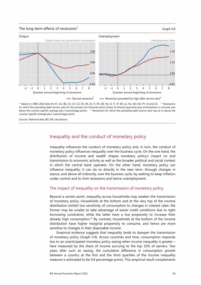
There is also evidence that financial recessions, even if they do not coincide with financial crises, are deeper and longer, and hence more costly in terms of inequality (Graph II.8). One way of seeing this is by considering recessions preceded by relatively high debt service ratios – a proxy for overindebtedness. The estimates suggest that eight quarters after the start of the recession, the average output drop is 2.5% larger and unemployment is 12% higher in financial recessions than in normal ones.

Inequality may not just amplify recessions; more subtly, it may also sow the seeds for them. For instance, it has been argued that higher inequality in the United States may have contributed to the build-up of housing debt. This was particularly the case for households with stagnating and less steady income, who were enticed into subprime borrowing. In turn, this higher leverage of households played a key amplifying role in the GFC, the archetypical “financial recession”. The reasoning is that low-income households have a larger need to borrow (eg to buy houses). If credit supply becomes more ample, this could encourage them to become overindebted. Down the road, an overburdened household sector can then trigger, or at least amplify, phases of weak economic activity. This impact is larger whenever the banking system comes under stress. Indeed, some observers have argued that this mechanism contributed to the subprime crisis that sparked off the GFC.15

Restricted

Chapter: xx


Stage: xx


Page/No of pp:

7/14



Higher income inequality leads to steeper declines in consumption Graph II.7

Recessions in more unequal countries lead to larger declines in consumption1

More unequal US states experienced larger declines in consumption during the GFC3

1 Estimated declines in real per capita private consumption during a recession at the specified percentile of income inequality. Recessionsare defined as a year of negative real GDP growth, and the share of income of the top 10% is taken as the indicator of income inequality.Estimates are based on a dynamic panel specification that includes country and time fixed effects. Specifically, real per capita privateconsumption growth is regressed on its lag, a recession dummy, the share of income held by the top 10% and the interaction between the latter two variables. Based on 1981–2019 data for 91 countries. Financial recessions are recessions that were associated with sovereign debt,banking or currency crises. For further details, see E Kohlscheen, M Lombardi and E Zakrajšek, “Income inequality and the depth of economicdownturns”, Economics Letters, vol 205, no 109934, August 2021. 2 Inequality taken from the sample distribution of the panel: low = 10th percentile; medium = 50th percentile; high = 90th percentile. 3 The vertical axis shows the residuals from the regression of state-level per capita private consumption growth between 2007 and 2009 on the change in unemployment and growth in house prices over the sameperiod; the horizontal axis shows the residuals from the regression of state-level income shares of the top 10% in 2006 on the change inunemployment and growth in house prices between 2007 and 2009. Based on all US states except District of Columbia.

Sources: World Bank; national data; BIS calculations.

–2

–4

–6

–8

–10

–12Financial recessionNormal recession

Low90% confidence interval

Inequality level:2 Medium High

Cons

umpt

ion

grow

th (%

) 3

0

–3

–6

–9

–12151050–5

Income share of top 10% (residuals, %)

Cons

umpt

ion

grow

th (r

esid

uals,

%)


Inequality and the conduct of monetary policy

Inequality influences the conduct of monetary policy and, in turn, the conduct of monetary policy influences inequality over the business cycle. On the one hand, the distribution of income and wealth shapes monetary policy’s impact on and transmission to economic activity as well as the broader political and social context in which the central bank operates. On the other hand, monetary policy can influence inequality: it can do so directly in the near term, through changes in stance; and above all indirectly, over the business cycle, by seeking to keep inflation under control and to limit recessions and hence unemployment.

The impact of inequality on the transmission of monetary policy

Beyond a certain point, inequality across households may weaken the transmission of monetary policy. Households at the bottom and at the very top of the income distribution exhibit low sensitivity of consumption to changes in interest rates: the former may be unable to take advantage of easier credit conditions due to tight borrowing constraints, while the latter have a low propensity to increase their already high consumption.16 By contrast, households at the bottom of the income distribution have higher marginal propensity to consume, and hence are more sensitive to changes in their disposable income.

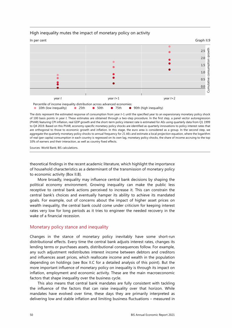
Empirical evidence suggests that inequality tends to dampen the transmission of monetary policy (Graph II.9). Across countries and time, consumption responds less to an unanticipated monetary policy easing when income inequality is greater – here measured by the share of income accruing to the top 10% of earners. Two years after such an easing, the cumulative difference in consumption growth between a country at the first and the third quartiles of the income inequality measure is estimated to be 0.8 percentage points. This empirical result complements

Restricted

Chapter: xx


Stage: xx


Page/No of pp:

6/11



The long-term effects of recessions1 Graph II.8

Output Unemployment Output index, excl government consumption Unemployment index

1 Based on 1980–2020 data for AT, AU, BE, CA, CH, CZ, DE, DK, ES, FI, FR, GB, HU, IE, IT, JP, KR, LU, NL, NO, NZ, PT, SE and US. 2 Recessions for which the preceding debt service ratio for the private non-financial sector (share of interest payments plus amortisations in income) was below the country-specific average plus 2 percentage points. 3 Recessions for which the preceding debt service ratio was at or above the country-specific average plus 2 percentage points.

Sources: National data; BIS; BIS calculations.

1.00

0.98

0.96

0.94876543210–1–2

Normal recession2

Quarters around beginning of recessions

1.30

1.15

1.00

0.85876543210–1–2

Recession preceded by high debt service ratio3



theoretical findings in the recent academic literature, which highlight the importance of household characteristics as a determinant of the transmission of monetary policy to economic activity (Box II.B).

More broadly, inequality may influence central bank decisions by shaping the political economy environment. Growing inequality can make the public less receptive to central bank actions perceived to increase it. This can constrain the central bank’s choices and eventually hamper its ability to achieve its mandated goals. For example, out of concerns about the impact of higher asset prices on wealth inequality, the central bank could come under criticism for keeping interest rates very low for long periods as it tries to engineer the needed recovery in the wake of a financial recession.

Monetary policy stance and inequality

Changes in the stance of monetary policy inevitably have some short-run distributional effects. Every time the central bank adjusts interest rates, changes its lending terms or purchases assets, distributional consequences follow. For example, any such adjustment redistributes interest income between debtors and creditors and influences asset prices, which reallocate income and wealth in the population depending on holdings (see Box II.C for a detailed analysis of this point). But the more important influence of monetary policy on inequality is through its impact on inflation, employment and economic activity. These are the main macroeconomic factors that shape inequality over the business cycle.

This also means that central bank mandates are fully consistent with tackling the influence of the factors that can raise inequality over that horizon. While mandates have evolved over time, these days they are primarily interpreted as delivering low and stable inflation and limiting business fluctuations – measured in

Restricted

Chapter: xx


Stage: xx


Page/No of pp:

7/11



High inequality mutes the impact of monetary policy on activity

In per cent Graph II.9

The dots represent the estimated response of consumption from year t–1 until the specified year to an expansionary monetary policy shockof 100 basis points in year t. These estimates are obtained through a two-step procedure. In the first step, a panel vector autoregression (PVAR) featuring CPI inflation, real GDP growth and the short-term policy interest rate is estimated for AEs using quarterly data from Q1 1999 to Q4 2019. Based on this PVAR, economy-specific monetary policy shocks are identified as quarterly innovations to policy interest rates thatare orthogonal to those to economic growth and inflation. In this stage, the euro area is considered as a group. In the second step, we aggregate the quarterly monetary policy shocks to annual frequency for 21 AEs and estimate a local projection equation, where the logarithmof real (per capita) consumption in each country is regressed on its own lag, monetary policy shocks, the share of income accruing to the top10% of earners and their interaction, as well as country fixed effects.

Sources: World Bank; BIS calculations.

2.5

2.0

1.5

1.0

0.5

0.0

year t year t+1 year t+2

10th (low inequality)Percentile of income inequality distribution across advanced economies:

25th

50th

75th

90th (high inequality)

Cum

ulat

ive

cons

umpt

ion

grow

th


terms of output and employment. And although financial stability need not be mentioned explicitly, it is naturally subsumed under the objective of smoothing fluctuations: just as price stability, financial stability is a necessary condition for output and employment to grow sustainably over time. This is true regardless of whether financial instability is interpreted narrowly – as banking or financial crises – or more broadly – as the amplification of business cycles and recessions induced by financial factors.17

Once high inflation or recessions materialise, the needed monetary response may have an undesirable short-run impact on inequality, in order to secure the long-term gains. Hence the importance of avoiding inflation and recessions in the first place.

Box II.BHeterogeneity and distribution in macroeconomic models

The growing focus on inequality in the economic debate has gone hand in hand with a change of perspective in macroeconomic modelling. Recent research has moved away from macroeconomic models based on a single representative agent and has focused instead on frameworks that incorporate heterogeneity in skills or wealth among households. This has allowed researchers to explore how inequality shapes macroeconomic outcomes and how macroeconomic shocks and stabilisation policies affect it. In these models – known as heterogeneous agent New Keynesian (HANK) models – several traditional policy prescriptions change when household heterogeneity is taken into account.

In traditional representative agent New Keynesian (RANK) models, monetary policy operates almost exclusively through a direct “real interest rate channel”: changes in the policy rate affect the real interest rate and induce households to reallocate consumption and saving over time. For instance, lower rates encourage them to bring consumption forward, reducing saving rates today. Yet empirical evidence shows that the response of consumption to monetary policy is mainly due to the indirect impact arising from an increase in employment and wages.

In RANK models, the impact of these indirect effects on consumption is small because the representative agent is generally assumed to be able to smooth consumption over time and is therefore not highly responsive to temporary income changes.

In HANK models, the direct impact from the “real interest rate channel” is small because a sizeable share of agents – especially those at the very bottom of the distribution – have negligible wealth. These agents’ consumption reacts little to changes in interest rates but is instead highly sensitive to changes in labour income (“labour income channel”). In addition, agents at the top of the wealth distribution hold equity and hence benefit from asset price increases (“equity price channel”) in response to an expansionary monetary policy.

Overall, the transmission of a monetary policy expansion can be weaker in HANK models than in RANK models. This depends on the distribution of income and wealth, and on other household characteristics that affect the relative strength of the different channels. The impact will be smaller in HANK if the “labour income channel” and the “equity price channel” are not strong enough to offset the weaker “real interest rate channel”.

In HANK models distributional factors also shape the optimal policy design: the main objective remains low and stable inflation, but the relative weight on unemployment in central banks’ strategy is higher. Considering inequality, a larger weight on unemployment stabilisation benefits the majority of households, as a more aggressive reaction to unemployment lowers earnings risk and precautionary savings by the employed and unemployed households at low and medium wealth deciles.

Models with heterogeneous agents featured prominently in the recent review of monetary policy strategy at the Federal Reserve; see L Feiveson, N Goernemann, J Hotchkiss, K Mertens and J Sim, “Distributional considerations for monetary policy strategy”, Board of Governors of the Federal Reserve System, Finance and Economics Discussion Series, no 2020-073, August 2020. See G Kaplan, B Moll and G Violante, “Monetary policy according to HANK”, American Economic Review, vol 108, no 3, pp 697–743, March 2018. See A Auclert, “Monetary policy and the redistribution channel”, American Economic Review, vol 109, no 6, pp 2333–67, June 2019. See N Gornemann, K Kuester and M Nakajima, “Doves for the rich, hawks for the poor? Distributional consequences of monetary policy”, Board of Governors of the Federal Reserve System, International Finance Discussion Papers, no 1167, May 2016.


Bringing inflation under control will generally call for a monetary policy tightening, which can induce recessions and hence increase income inequality. In AEs, a clear example is the “Volcker shock” of the early 1980s in the United States, which set the basis for the conquest of inflation. In EMEs, the episodes are more common and severe. For instance, the Central Bank of Brazil had to raise the policy rate by more than 10 percentage points between 2001 and 2003 to rein in a surge in inflation.

Similarly, sustaining a recovery in the aftermath of a severe economic recession requires keeping interest rates low for longer, especially if they are constrained by the effective lower bound.18 For example, had monetary policy refrained from deploying all necessary tools to keep borrowing costs low in the aftermath of the GFC and the Covid-19 pandemic, the recessions would have been deeper and longer. This, in turn, would have exposed the most disadvantaged to longer

Box II.CThe impact of interest rates on wealth inequality

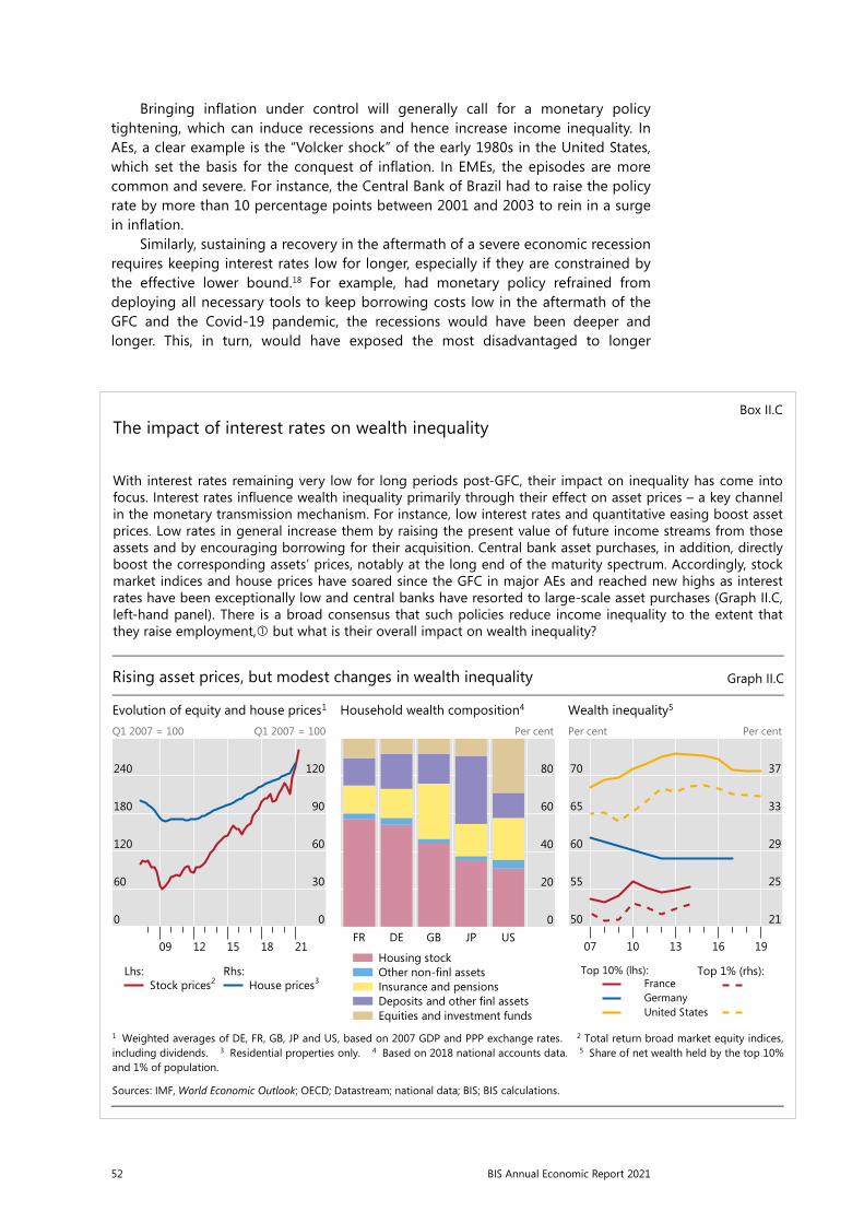
With interest rates remaining very low for long periods post-GFC, their impact on inequality has come into focus. Interest rates influence wealth inequality primarily through their effect on asset prices – a key channel in the monetary transmission mechanism. For instance, low interest rates and quantitative easing boost asset prices. Low rates in general increase them by raising the present value of future income streams from those assets and by encouraging borrowing for their acquisition. Central bank asset purchases, in addition, directly boost the corresponding assets’ prices, notably at the long end of the maturity spectrum. Accordingly, stock market indices and house prices have soared since the GFC in major AEs and reached new highs as interest rates have been exceptionally low and central banks have resorted to large-scale asset purchases (Graph II.C, left-hand panel). There is a broad consensus that such policies reduce income inequality to the extent that they raise employment, but what is their overall impact on wealth inequality?

Restricted

Chapter: xx


Stage: xx


Page/No of pp:

10/11



Rising asset prices, but modest changes in wealth inequality Graph II.C

Evolution of equity and house prices1 Household wealth composition4 Wealth inequality5 Q1 2007 = 100 Q1 2007 = 100 Per cent Per cent Per cent

1 Weighted averages of DE, FR, GB, JP and US, based on 2007 GDP and PPP exchange rates. Total return broad market equity indices, 2

including dividends. 3 Residential properties only. 4 Based on 2018 national accounts data. 5 Share of net wealth held by the top 10%and 1% of population.

Sources: IMF, World Economic Outlook; OECD; Datastream; national data; BIS; BIS calculations.

240

180

120

60

0

120

90

60

30

0

2118151209

Stock prices2Lhs:

House prices3Rhs:

80

60

40

20

0USJPGBDEFR

Housing stockOther non-finl assetsInsurance and pensionsDeposits and other finl assetsEquities and investment funds

70

65

60

55

50

37

33

29

25

21

1916131007

France Germany United States

Top 10% (lhs):

Top 1% (rhs):


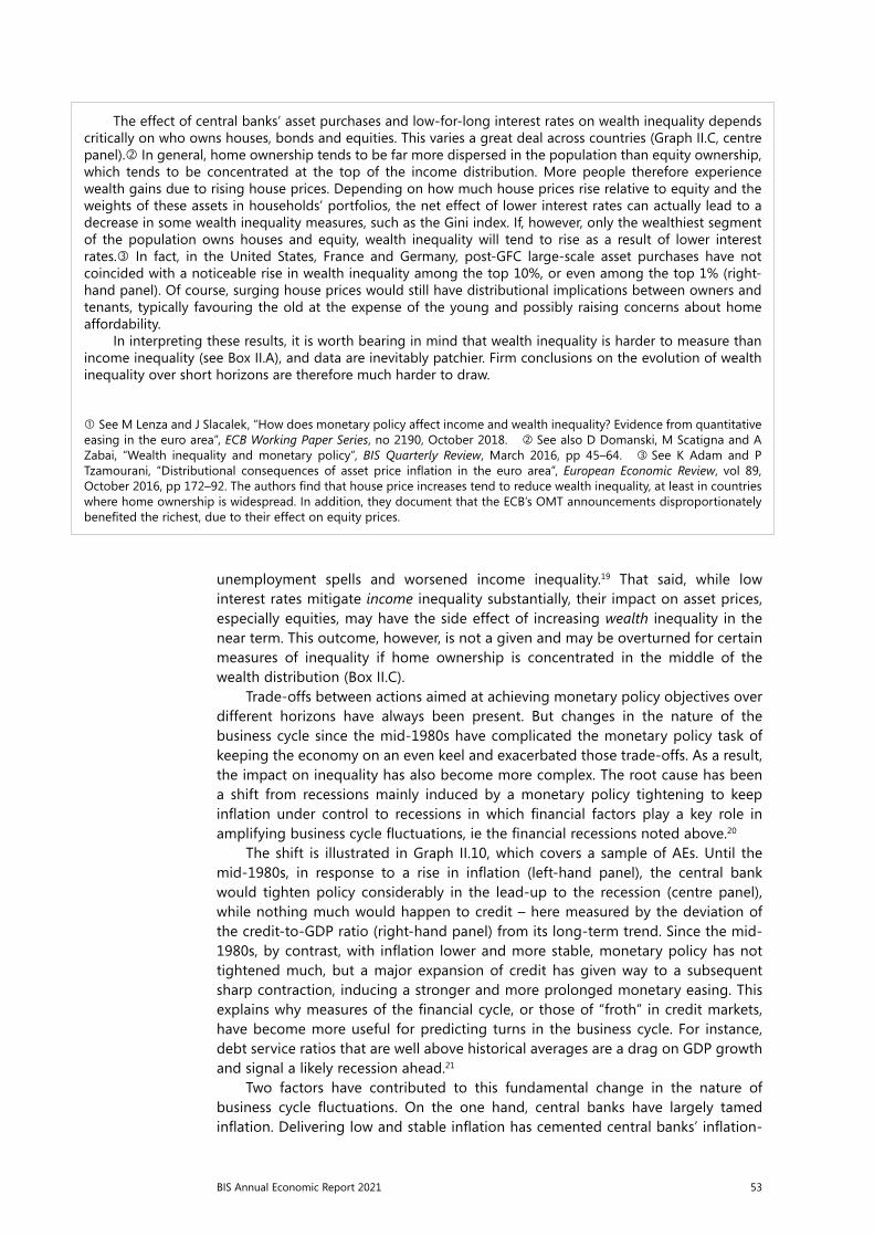
The effect of central banks’ asset purchases and low-for-long interest rates on wealth inequality depends critically on who owns houses, bonds and equities. This varies a great deal across countries (Graph II.C, centre panel). In general, home ownership tends to be far more dispersed in the population than equity ownership, which tends to be concentrated at the top of the income distribution. More people therefore experience wealth gains due to rising house prices. Depending on how much house prices rise relative to equity and the weights of these assets in households’ portfolios, the net effect of lower interest rates can actually lead to a decrease in some wealth inequality measures, such as the Gini index. If, however, only the wealthiest segment of the population owns houses and equity, wealth inequality will tend to rise as a result of lower interest rates. In fact, in the United States, France and Germany, post-GFC large-scale asset purchases have not coincided with a noticeable rise in wealth inequality among the top 10%, or even among the top 1% (right-hand panel). Of course, surging house prices would still have distributional implications between owners and tenants, typically favouring the old at the expense of the young and possibly raising concerns about home affordability.

In interpreting these results, it is worth bearing in mind that wealth inequality is harder to measure than income inequality (see Box II.A), and data are inevitably patchier. Firm conclusions on the evolution of wealth inequality over short horizons are therefore much harder to draw.

See M Lenza and J Slacalek, “How does monetary policy affect income and wealth inequality? Evidence from quantitative easing in the euro area”, ECB Working Paper Series, no 2190, October 2018. See also D Domanski, M Scatigna and A Zabai, “Wealth inequality and monetary policy”, BIS Quarterly Review, March 2016, pp 45–64. See K Adam and P Tzamourani, “Distributional consequences of asset price inflation in the euro area”, European Economic Review, vol 89, October 2016, pp 172–92. The authors find that house price increases tend to reduce wealth inequality, at least in countries where home ownership is widespread. In addition, they document that the ECB’s OMT announcements disproportionately benefited the richest, due to their effect on equity prices.

unemployment spells and worsened income inequality.19 That said, while low interest rates mitigate income inequality substantially, their impact on asset prices, especially equities, may have the side effect of increasing wealth inequality in the near term. This outcome, however, is not a given and may be overturned for certain measures of inequality if home ownership is concentrated in the middle of the wealth distribution (Box II.C).

Trade-offs between actions aimed at achieving monetary policy objectives over different horizons have always been present. But changes in the nature of the business cycle since the mid-1980s have complicated the monetary policy task of keeping the economy on an even keel and exacerbated those trade-offs. As a result, the impact on inequality has also become more complex. The root cause has been a shift from recessions mainly induced by a monetary policy tightening to keep inflation under control to recessions in which financial factors play a key role in amplifying business cycle fluctuations, ie the financial recessions noted above.20

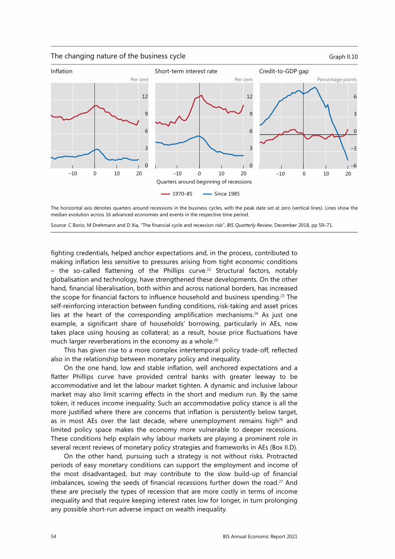
The shift is illustrated in Graph II.10, which covers a sample of AEs. Until the mid-1980s, in response to a rise in inflation (left-hand panel), the central bank would tighten policy considerably in the lead-up to the recession (centre panel), while nothing much would happen to credit – here measured by the deviation of the credit-to-GDP ratio (right-hand panel) from its long-term trend. Since the mid-1980s, by contrast, with inflation lower and more stable, monetary policy has not tightened much, but a major expansion of credit has given way to a subsequent sharp contraction, inducing a stronger and more prolonged monetary easing. This explains why measures of the financial cycle, or those of “froth” in credit markets, have become more useful for predicting turns in the business cycle. For instance, debt service ratios that are well above historical averages are a drag on GDP growth and signal a likely recession ahead.21

Two factors have contributed to this fundamental change in the nature of business cycle fluctuations. On the one hand, central banks have largely tamed inflation. Delivering low and stable inflation has cemented central banks’ inflation-


fighting credentials, helped anchor expectations and, in the process, contributed to making inflation less sensitive to pressures arising from tight economic conditions – the so-called flattening of the Phillips curve.22 Structural factors, notably globalisation and technology, have strengthened these developments. On the other hand, financial liberalisation, both within and across national borders, has increased the scope for financial factors to influence household and business spending.23 The self-reinforcing interaction between funding conditions, risk-taking and asset prices lies at the heart of the corresponding amplification mechanisms.24 As just one example, a significant share of households’ borrowing, particularly in AEs, now takes place using housing as collateral; as a result, house price fluctuations have much larger reverberations in the economy as a whole.25

This has given rise to a more complex intertemporal policy trade-off, reflected also in the relationship between monetary policy and inequality.

On the one hand, low and stable inflation, well anchored expectations and a flatter Phillips curve have provided central banks with greater leeway to be accommodative and let the labour market tighten. A dynamic and inclusive labour market may also limit scarring effects in the short and medium run. By the same token, it reduces income inequality. Such an accommodative policy stance is all the more justified where there are concerns that inflation is persistently below target, as in most AEs over the last decade, where unemployment remains high26 and limited policy space makes the economy more vulnerable to deeper recessions. These conditions help explain why labour markets are playing a prominent role in several recent reviews of monetary policy strategies and frameworks in AEs (Box II.D).

On the other hand, pursuing such a strategy is not without risks. Protracted periods of easy monetary conditions can support the employment and income of the most disadvantaged, but may contribute to the slow build-up of financial imbalances, sowing the seeds of financial recessions further down the road.27 And these are precisely the types of recession that are more costly in terms of income inequality and that require keeping interest rates low for longer, in turn prolonging any possible short-run adverse impact on wealth inequality.

Restricted

Chapter: xx


Stage: xx


Page/No of pp:

8/11



The changing nature of the business cycle Graph II.10

Inflation Short-term interest rate Credit-to-GDP gap Per cent Per cent Percentage points

The horizontal axis denotes quarters around recessions in the business cycles, with the peak date set at zero (vertical lines). Lines show the median evolution across 16 advanced economies and events in the respective time period.

Source: C Borio, M Drehmann and D Xia, “The financial cycle and recession risk”, BIS Quarterly Review, December 2018, pp 59–71.

12

9

6

3

020100–10

12

9

6

3

020100–10

1970–85 Since 1985


6

3

0

–3

–6 20 10 0–10


Box II.DLabour markets and the reviews of monetary policy frameworks

Against the backdrop of the changing nature of business cycles, and capitalising on the lessons learnt since the GFC, several central banks in major AEs recently launched reviews of their monetary policy frameworks. The aim was to assess the adequacy of strategies and monetary policy instruments to achieve the mandated objectives. The Federal Reserve was the first, launching its review in 2019 and completing it in August 2020. The ECB and the Bank of Canada have also embarked on similar reviews, which are planned to be concluded in the second half of 2021.

Labour markets have played a prominent role in these reviews – especially in the case of the Federal Reserve. To be sure, the Fed’s reading of labour markets had been evolving for quite some time. For example, in a 2016 speech, Chair Yellen argued that running the economy at “high-pressure” could be a powerful tool to reverse the labour market hysteresis – a surge in unemployment coupled with a drop in participation rates – that followed the GFC. In the wake of such considerations, the strategy review downplayed the concept of the “natural” rate of unemployment – ie the level above which the labour market is overheated and inflation should increase. Such a “natural” rate of unemployment cannot be observed directly and needs to be estimated using various econometric techniques. Many approaches actually rely on the empirical relationship of unemployment and inflation, which has weakened over time.

In a context in which the natural rate of unemployment plays little role, inflation takes centre stage as a gauge of economic overheating. To the extent that inflation remains low, central banks can afford to let labour markets tighten. Due to the flattening of the Phillips curve, tighter labour markets may produce limited price pressures, so that inflation may well remain below target. To strengthen the commitment to delivering inflation at target, the review has led to the adoption of a flexible form of average inflation targeting. Following a period of below-target inflation, the central bank commits to keep an easier stance for longer, while it waits for the backward-looking average of actual inflation to reach the target. This may require inflation to “overshoot” the target by an amount and a duration that depends on the previously experienced undershooting. An accommodative monetary policy, in turn, will stimulate demand and output, to the point of enticing the discouraged workers back into the labour force. This should have a positive effect on potential output and further sustain inflation.

The Fed’s new strategy is intended to bring benefits in terms of a more equitable income distribution. A tight labour market can facilitate the inclusion in the labour force of the most disadvantaged segments of the population, lifting them out of poverty and marginalisation. Hence, on top of boosting potential growth, a wider labour force participation and more employment opportunities should dampen income inequality by boosting the income of the poorest.

The current review of the monetary policy framework at the Bank of Canada shares with the Fed’s review a broader set of criteria than in the past against which to evaluate possible alternative frameworks. In particular, those criteria now also include the impact on the distribution of income and wealth. The European Central Bank is also analysing a wide range of topics, many of which have important links to inequality. These include employment, digitalisation, globalisation, productivity, innovation and technological progress. Moreover, in early 2020, the ECB held a series of events with the general public to gather suggestions. A notable one was that the ECB should consider a direct way for its policies to have an impact on people, rather than through banks and financial institutions.

This is also because, at the time of writing, the strategy reviews in other central banks were already ongoing, so the information available was more limited. See J Yellen, “Macroeconomic research after the crisis“, speech at the 60th annual economic conference sponsored by the Federal Reserve Bank of Boston, 14 October 2016. This reasoning is consistent with the “plucking” theory of the business cycle in which employment, rather than hovering around a certain equilibrium level, is capped by a certain maximum level. According to this theory, the Phillips curve has a non-linear shape, so that inflation pressures only kick in in the proximity of the maximum attainable level of employment. See S Dupraz, E Nakamura and J Steinsson, “A plucking model of business cycles”, NBER Working Papers, no 26351, October 2019. See, for example, M Daly, “Is the Federal Reserve contributing to economic inequality?”, speech at UC Irvine, 16 October 2020. See C Wilkins, “Toward the 2021 renewal of the monetary policy framework”, opening remarks of the Bank of Canada Workshop, 26 August 2020. See C Lagarde, “The monetary policy strategy review: some preliminary considerations”, speech at the “ECB and Its Watchers XXI” conference, 30 September 2020.


The trickier nature of the intertemporal trade-offs linked to the nature of the business cycle has complicated monetary policy’s task of fulfilling its objectives. It has become harder to reconcile price with financial, and hence macroeconomic, stability in the near term. As a result, the consequences for inequality have also become larger. Monetary policy cannot adequately handle these intertemporal trade-offs on its own. As discussed next in more detail, they call for a more balanced policy approach in which other policies, notably prudential, fiscal and structural, also play a role.

Beyond monetary policy

The previous analysis indicates that the best contribution monetary policy can make to a more equitable distribution of income and wealth is to deliver on its mandate – seeking to ensure macroeconomic stability, for which price and financial stability are prerequisites. By keeping the economy on an even keel, central banks facilitate sustainable growth. The benefits of doing so are first-order.

It would be unrealistic, and indeed counterproductive, to gear monetary policy more squarely towards tackling inequality. Monetary tools, by their very nature, act primarily on cyclical developments. That is why they are well suited to achieving macroeconomic stabilisation objectives. By contrast, a meaningful impact on slow-moving inequality trends would entail sustained application of the tools in particular ways. This would curtail the flexibility of monetary policy to stabilise the economy, potentially undermining the effectiveness of the monetary regime itself. This would be very costly, not least because the macroeconomic stability that those regimes can deliver is precisely what is most conducive to equitable income and wealth distributions.

With monetary policy playing a supportive role, other policies are, therefore, critical. Three types of policy deserve attention: those that complement monetary policy in delivering macroeconomic stability in the different phases of the business cycle; those that address structural inequality; and those that central banks can deploy in fulfilment of their non-monetary policy responsibilities.

Macroeconomic stability

While monetary policy plays a key role in promoting macroeconomic stability, it cannot deliver it on its own. This is true regardless of the nature of the business cycle. It is well known, for instance, that fiscal sustainability is a prerequisite for macroeconomic stability, and that it can be especially constraining in EMEs (Chapter I). But changes in the nature of the business cycle have brought the limits of what monetary policy can do into starker relief. In order to better understand the need for complementary policies, consider a stylised business cycle associated with a financial recession.

During the expansionary phase of the business cycle, even if monetary policy keeps inflation in check, vulnerabilities may build up in the financial system as the financial cycle gathers momentum. This is because credit and asset prices can grow rapidly boosted by high risk-taking, so that balance sheets may become overstretched. Macroprudential measures can play a key role here. They can seek to slow down the financial expansion and restrain risk-taking, especially in the sectors deemed to pose the bigger risks to the financial system (Chapter I).

The role of microprudential policies, which are structural in nature and not aimed at smoothing the financial cycle per se, becomes evident once the recession sets in. Adequate microprudential safeguards must be in place so that the banking


system is resilient going into the downturn and can better support the economy. This is precisely what the post-GFC major international prudential reforms – notably Basel III – did pre-Covid. The reforms allowed banks to avoid deleveraging and to better support credit, thereby cushioning the blow to the economy (Chapter I).

That said, if the financial imbalances are large enough, the prudential safeguards may not be sufficient to prevent more widespread and intense financial stress. At this point, monetary policy enters crisis management mode, with central banks acting as lenders and, increasingly, as market-makers of last resort.28 This may make central banks the target of criticism for favouring “Wall Street” at the expense of “Main Street”. But this is a false dichotomy, as such actions are necessary to prevent greater damage. A collapse of the financial system would curtail credit to business and households and spawn a deep recession, at great cost in terms of unemployment and income inequality. Also on this front, however, central banks cannot succeed on their own: fiscal backstops are essential to stabilise banks, the overall financial system and thereby the economy. In addition, government intervention to help repair balance sheets is critical to resolve the crisis and set the basis for a healthy recovery.

As financial conditions stabilise, the challenge becomes nursing the recovery and battling the headwinds of a debt overhang. Monetary policy accommodation can help mitigate the recession and speed up the recovery, but a balanced mix of monetary, fiscal and structural policies is called for to prevent central banks from becoming “the only game in town”. Fiscal policy can ease the burden on central banks and attenuate the impact of recessions on inequality. Automatic stabilisers are useful but may need to be complemented with discretionary measures. For example, thanks to sizeable income transfers, personal disposable income in most countries has actually grown faster (or declined less) than wage income during the pandemic (Chapter I, Graph I.2, left-hand panel). At the same time, it is essential that fiscal policy be run prudently to prevent it from becoming a source of macroeconomic instability. Imprudent fiscal policies can raise risk premia, fuel currency depreciation and eventually destabilise the economy, not least by generating full-blown financial crises. Structural policies are also important in this context, as they are the sole engine of sustainable longer-term growth, which cannot rely on persistent fiscal and monetary stimulus.

Structural inequality

Addressing the structural trends in inequality is first and foremost a task for governments. They can avail themselves of a better and broader set of tools to tackle inequality, ranging from taxation to transfers as well as to policies aimed at improving education, property rights, health, competition and trade, among others. Moreover, politically, governments bear the responsibility for achieving a desirable distribution of resources.

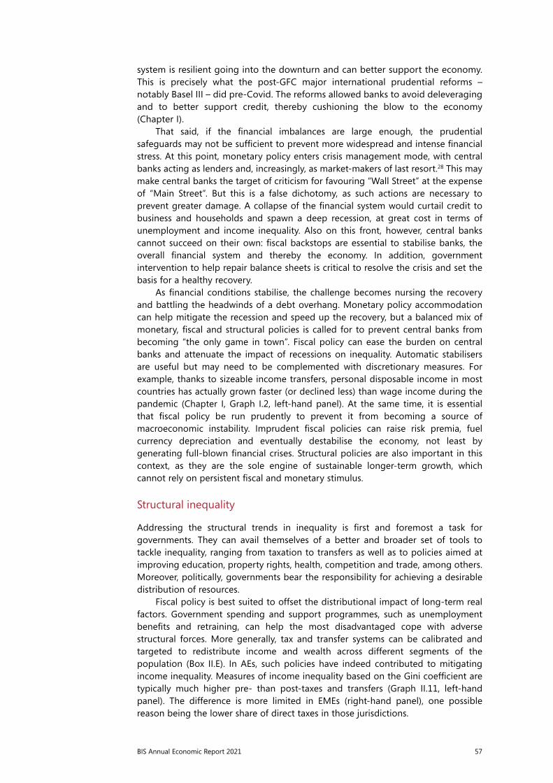
Fiscal policy is best suited to offset the distributional impact of long-term real factors. Government spending and support programmes, such as unemployment benefits and retraining, can help the most disadvantaged cope with adverse structural forces. More generally, tax and transfer systems can be calibrated and targeted to redistribute income and wealth across different segments of the population (Box II.E). In AEs, such policies have indeed contributed to mitigating income inequality. Measures of income inequality based on the Gini coefficient are typically much higher pre- than post-taxes and transfers (Graph II.11, left-hand panel). The difference is more limited in EMEs (right-hand panel), one possible reason being the lower share of direct taxes in those jurisdictions.


Mitigating inequality also requires well designed growth-promoting structural policies. There is a range of relevant measures.

First and foremost, policies designed to improve access to, and the quality of, education and on-the-job learning are crucial to keep pace with rapid technological change. Such policies do not just raise output by increasing human capital and productivity; they also help level the playing field and reduce inequality by providing access to better-paid job opportunities.29

Labour market and competition policies sustain growth and also help tackle the challenges brought about by technological change and changes in the composition of demand in favour of high-skilled jobs. Easing re-entry of the long-term unemployed, typically the less skilled, into labour markets can reduce the income gap vis-à-vis higher-skilled workers. And labour market regulation can ensure minimum standards for wages and unemployment benefits, rebalancing bargaining power.

Trade openness can also contribute, especially for lower-income countries benefiting from the extra foreign demand. But it needs to be combined with proper compensation, retraining and reallocation policies for those who are displaced.30 Evidence indicates that, absent redistribution policies, the removal of tariffs on agricultural and manufacturing goods increases aggregate output at the cost of an initial rise in income inequality.31

Central banks’ non-monetary hats

Central banks can also contribute to a more equitable society wearing their “non-monetary hats”. These are functions attributed to them by statute beyond their monetary policy mandate.

The previous analysis has already discussed the important role of financial stability-related functions for inequality, including micro- and macroprudential regulation and supervision and those concerned with crisis management. But many more are relevant in this context: fostering financial development; furthering financial inclusion; protecting consumers of financial services; encouraging financial

Restricted

Chapter: xx


Stage: xx


Page/No of pp:

11/14



Fiscal policy redistributes income

Gini index Graph II.11

Advanced economies1 Emerging market economies2

1 For CA, DE, GB and US, 2018; for FR, 2012; for IT, 2017; for JP, 2015. 2 For BR, 2014; for CN, 2015; for IN, 2013; for RU and ZA, 2018.

Sources: Luxembourg Income Study (LIS) Database; Standardized World Income Inequality Database (SWIID); BIS calculations.

60

40

20

0

CAGBFRJPUSDEIT

Pre-tax, pre-transfer incomeGini index in:

60

40

20

0

RUCNINBRZA

Post-tax, post-transfer income


Restricted

Chapter: xx


Stage: xx


Page/No of pp:

11/11



Different fiscal policy tools can shape different parts of the income distribution Graph II.E

Evolution of tax rate progressivity and public transfers

Higher tax progressivity comes with lower inequality at the top…3

…while higher transfers come with lower inequality at the bottom4

Percentage points Percentage of GDP

1 Tax progressivity is estimated for each country-year pair by regressing average tax rates on log-personal income. Personal income levels are defined as multiples of current GDP per capita, starting from 4% and ending at 400% with increments of 4 percentage points, making 100 hypothetical income levels for each country and year. Country sample: 27 AEs and eight EMEs. See D Duncan and K Sabirianova Peter, “Unequal inequalities: do progressive taxes reduce income inequality?”, IZA Discussion Papers, no 6910, October 2012. Corresponding average tax rates are computed using OECD data on personal income tax rates and thresholds. 2 As a share of current GDP. 3 Partial correlation estimated by regressing the ratio of the 90th income percentile to the 50th income percentile for a panel of countries and incomes over the period2000–19 on tax progressivity and average tax burden as well as lagged Gini index. The regression is estimated including country and time fixed effects. Country sample: AT, BE, CA, CH, CZ, DE, DK, ES, FI, FR, GB, IE, IT, KR, NL, NO, PT, SE and US. 4 Partial correlation estimated by regressing the ratio of the 50th income percentile to the 10th income percentile for a panel of countries and incomes over the period 2000–19on the yearly change in public transfers as a share of current GDP, controlling for the lagged dependent variable. The regression is estimated including country and time fixed effects. Country sample: AT, BE, CA, CH, DE, DK, ES, FI, FR, GB, IT, NL, NO, SE and US.

Sources: OECD, Economic Outlook and Tax Database; Standardized World Income Inequality Database (SWIID); UNU-WIDER, World Income Inequality Database (WIID); BIS calculations.

7.0

6.5

6.0

5.5

14

13

12

112015100500

Tax rate progressivity1 (lhs)Public transfers2 (rhs)

0.1

0.0

–0.1

–0.20.0040.0020.000–0.002

(residuals)Personal income tax progressivity

90th

/50t

h in

com

e pe

rcen

tiles

(res

idua

ls)

0.1

0.0

–0.1

–0.20.0100.0050.000–0.005

(residuals)Change in public transfers to GDP

50th

/10t

h in

com

e pe

rcen

tiles

(res

idua

ls)

Box II.EFiscal policy and inequality

Governments can affect inequality using a number of different fiscal policy tools. On the revenue side, they can influence the income distribution by changing income taxes. Progressive taxation, which imposes higher tax rates on higher-income households, can reduce after-tax income inequality. Similarly, taxes on wealth or inheritance can reduce after-tax wealth inequality. On the expenditure side, governments can direct public transfers towards specific segments of the population to affect their disposable income and hence inequality. For instance, unemployment insurance can significantly limit the impact of recessions on inequality by sustaining the income of workers who lose their job. Public transfers also tend to reduce inequality since they usually aim to ensure minimum living standards, thereby disproportionately benefiting the poor.

Changes in taxes and transfers have had a differential direct impact on inequality. On the one hand, personal income tax progressivity has declined globally (Graph II.E, left-hand panel). The decrease of about 1.5 percentage points over the past two decades amounts to a noticeable reduction in the tax burden of the highest-income households. On the other hand, public transfers as a share of GDP increased significantly in the wake of the GFC. They have declined somewhat since then but have remained notably above pre-GFC levels.

Cross-country evidence confirms that a higher degree of tax progressivity is associated with lower inequality, particularly at the top of the income distribution (Graph II.E, centre panel). A reduction in tax progressivity of the same order of magnitude as observed over the past two decades is associated with an increase of about 11 percentage points in the share of income of the top 10% of earners relative to the median income earners.

For their part, public transfers help reduce inequality at the bottom of the distribution. Cross-country evidence shows that increases in public transfers as a share of GDP are associated with lower inequality in the


literacy and education; and overseeing payment systems.32 The extent to which central banks can contribute to fighting inequality performing these tasks naturally depends on their statutory responsibilities, which vary substantially across countries, and, importantly, on the range and effectiveness of the tools at their disposal.

The beneficial impact of these policies on inequality is multifaceted. Fostering financial development can widen the menu of options to hedge and diversify risks, enhancing investment opportunities and mitigating poverty and income inequality.33 Promoting financial inclusion by providing safe savings vehicles or smooth payment infrastructures expands financial market access for the most disadvantaged, particularly in poorer countries.34 Financial services consumer protection shields the poor and more vulnerable from predatory lending35 and, together with financial literacy and education, from excessive risk-taking. Spearheading efforts to develop safe, smooth and competitive payment systems not only underpins financial stability; it also helps reduce overall costs, not least for cross-border remittances.

Conclusion

Inequality is largely the result of long-term structural forces that are independent of monetary policy. Over the past few decades, globalisation and technology have played a prominent role. Policies that foster more equal opportunities or redistribute income are best suited to counteract the impact of long-term forces on income and wealth inequality. Structural policies, including those targeted to education, health and competition, give the relatively poor of today the instruments to become the well-off of tomorrow, promoting social mobility and equitable growth. Fiscal policies, notably through redistribution, help correct the uneven distribution of the aggregate gains from growth.

Monetary policy does not have adequate tools to offset the long-term distributional consequences of evolving structural factors. Nevertheless, depending on statutory responsibilities, central banks can make a significant contribution by wearing their “non-monetary hats”, to an extent that depends on the tools available. Promoting financial development, inclusion and literacy, protecting against unfair financial practices, and furthering low-cost payment services all contribute to a more equitable society.

This is not to say that monetary policy cannot foster a more equitable society; far from it. Monetary policy can make an important contribution by keeping the economy on an even keel in fulfilment of its mandate, ie by tackling macroeconomic, including financial, instability. Macroeconomic instability can have a first-order

bottom half of the income distribution (Graph II.E, right-hand panel). This empirical regularity probably reflects changes in public transfers disproportionately benefiting the poor, especially as transfers tend to increase more steeply during recessions. Accordingly, increases in transfers have little impact at the top of the income distribution.

The variety of fiscal policy tools available to governments gives them significant scope to address inequality arising from different segments of the income distribution, and nudge it towards the desired outcome.

Consistent longer-term evidence is provided in T Piketty, E Saez and G Zucman, “Distributional national accounts: methods and estimates for the United States”, The Quarterly Journal of Economics, vol 133, no 2, May 2018, pp 553–609. See also D Denvil and K Sabirianova Peter, “Unequal inequalities: do progressive taxes reduce income inequality?”, International Tax and Public Finance, vol 23, no 4, August 2016, pp 762–83. See I Joumard, M Pisu and D Bloch, “Tackling income inequality: the role of taxes and transfers“, OECD Journal: Economic Studies, vol 2012, no 1, 2012.

https://link.springer.com/journal/10797


impact on inequality over business cycle fluctuations. The two major forms of instability are high inflation, which disproportionately erodes income of households at the bottom of the distribution, and recessions, which hurt the poor through unemployment spells.

Changes in the nature of the business cycle over the recent decades have complicated monetary policy’s ability to counteract macroeconomic instability and its impact on inequality. To be sure, inflation has largely been conquered – a major achievement. But financial factors have come to the fore as a key force amplifying business cycle fluctuations. Financial recessions tend to be deeper and longer, especially if a financial crisis breaks out, and therefore much more costly in terms of inequality. Moreover, they require the central bank to keep interest rates low for longer to nurture a recovery: by boosting asset prices, especially those of equities, this may raise wealth inequality in the short run even as it delivers substantial benefits by bolstering employment and reducing income inequality. The intertemporal trade-offs that arise pose a key challenge. With inflation less responsive to economic slack, the central bank can keep the monetary policy stance easier for longer. This brings more people into the labour force, supports employment and reduces inequality. But it may also contribute to a slow build-up of financial imbalances that sow the seeds of costlier financial recessions down the road.

In order to better address these trade-offs, a more balanced policy approach is needed. Prudential, fiscal and structural policies are important in this context, as part of a comprehensive macro-financial stability framework.


Endnotes1 Unless otherwise specified, the chapter focuses on measures of inequality before redistributive

actions taken by governments, eg taxes and transfers. The impact of these on inequality is discussed in detail in the last section.

2 See also A Atkinson and F Bourguignon, Handbook of income distribution, vol 2, Elsevier, 2015.

3 For a survey of different approaches, see M Ravaillon, “Poverty lines across the world”, World Bank Policy Research Working Papers, no 5284, April 2010.

4 See eg D Acemoglu, “Technical change, inequality and the labor market”, Journal of Economic Literature, vol 40, no 1, March 2002, pp 7–72; and F Bourguignon, The globalization of inequality, Princeton University Press, 2015.

5 For a survey of the academic literature on skill-biased technical change, see N Chusseau, M Dumont and J Hellier, “Explaining rising inequality: skill-biased technical change and north-south trade”, Journal of Economic Surveys, vol 22, no 3, July 2008, pp 409–57.

6 See D Autor, D Dorn, L Katz, C Patterson and J Van Reenen, “The fall of the labor share and the rise of superstar firms”, The Quarterly Journal of Economics, vol 135, no 2, May 2020, pp 645–709.

7 On this, see eg A Atkinson, Inequality: what can be done?, Harvard University Press, 2015.

8 See J Tinbergen, “Substitution of graduate by other labour”, Kyklos, vol 27, no 2, January 1974, pp 217–26.

9 See A Carstens, “Central banks and inequality”, remarks at Princeton University’s Bendheim Center for Finance, 6 May 2021.

10 See D Krueger, K Mitman and F Perri, “On the distribution of the welfare losses of large recessions”, NBER Working Papers, no 22458, July 2016.

11 See eg S Fischer, R Sahay and C Vegh, “Stabilization and growth in transition economies: the early experience”, Journal of Economic Perspectives, vol 10, no 2, spring 1996, pp 45–66.

12 The significant interplay between inflation and income inequality in EMEs probably reflects the importance of the informal sector, as workers relying mostly on cash payments are particularly exposed to inflation. In AEs, by contrast, greater participation in banking services and higher financial literacy may enable more inflation hedging opportunities.

13 On the link between recessions and inequality, see D Krueger et al, op cit.

14 See E Kohlscheen, M Lombardi and E Zakrajšek, “Income inequality and the depth of economic downturns”, Economics Letters, vol 205, no 109934, August 2021.

15 R Rajan, Fault lines: how hidden fractures still threaten the world economy, Princeton University Press, 2011.

16 See G Kaplan, B Moll and G Violante, “Monetary policy according to HANK”, American Economic Review, vol 108, no 3, March 2018, pp 697–743.

17 On the financial amplification of business cycles, see R Kollmann, “Global banks, financial shocks, and international business cycles: evidence from an estimated model”, Journal of Money, Credit and Banking, vol 45, no 2, December 2013, pp 159–95; and M Iacoviello, “Financial business cycles”, Review of Economic Dynamics, vol 18, no 1, January 2015, pp 140–63.

18 Beyond the cyclical evolution of interest rates, there is a deeper question about the long-term drivers of the fall in real interest rates since the 1980s. Clearly, the real rates consistent with stable inflation and output at potential have declined – what is commonly referred to as r-star or the natural rate of interest. There is a large body of evidence indicating that the main forces at work have been of a structural nature, including factors such as demographics, long-term growth, a growing wedge between the required return on capital and the risk-free rate, the relative price


of capital and inequality itself, among others, all of which hardly depend on monetary policy. See eg M Marx, B Mojon and F Velde, “Why have interest rates fallen far below the return on capital?”, BIS Working Papers, no 794, July 2019; and L Rachel and T Smith, “Are low real interest rates here to stay?”, International Journal of Central Banking, vol 13, no 3, September 2017, pp 1–42 for recent surveys of the evidence. Some of the empirical work on the determinants of real rates finds much weaker evidence for such a link with those specific factors; see eg K Lunsford and K West, “Some evidence on secular drivers of US safe real rates”, American Economic Journal: Macroeconomics, vol 11, no 4, 2019, pp 113–39; and C Borio, P Disyatat, M Juselius and P Rungcharoenkitkul, “Why so low for so long? A long-term view of real interest rates”, BIS Working Papers, no 685, December 2017; forthcoming in the International Journal of Central Banking.

19 See eg M Lenza and J Slacalek, “How does monetary policy affect income and wealth inequality? Evidence from quantitative easing in the euro area”, ECB Working Paper Series, no 2190, October 2018. The authors estimate that in the absence of a quantitative easing impulse in the euro area, the unemployment rate would have been up to 0.7 percentage points higher on average. This would have implied a loss of 1.1 million jobs.

20 See eg Box I.B in BIS, Annual Economic Report, June 2018.

21 C Borio, M Drehmann and D Xia, “Predicting recessions: financial cycle versus term spread”, BIS Working Papers, no 818, October 2019.

22 The flattening of the Phillips curve may have been produced by secular trends such as globalisation, technology and the related erosion of workers’ bargaining power (see eg BIS, 84th Annual Report, June 2014, Chapter III) and/or by more firmly anchored inflation expectations due to successful monetary policy (see eg M McLeay and S Tenreyro, ”Optimal inflation and the identification of the Phillips curve”, NBER Macroeconomics Annual, 2019).

23 Demirgüç-Kunt and Detragiache (1998) time the start of financial liberalisations in most AEs to before 1985. See A Demirgüç-Kunt and E Detragiache, “Financial liberalization and financial fragility”, IMF Working Papers, no 98/83, June 1998.

24 See C Borio, C Furfine and P Lowe, “Procyclicality of the financial system and financial stability: issues and policy options”, BIS Papers, no 1, March 2001; and V Bruno and H S Shin, “Cross-border banking and global liquidity”, Review of Economic Studies, vol 82, no 2, April 2015, pp 535–64.

25 See S Claessens, M Kose and M Terrones, “How do business and financial cycles interact?”, Journal of International Economics, vol 87, no 1, May 2012, pp 178–90; and O Jordá, M Schularick and A Taylor, “When credit bites back”, Journal of Money, Credit and Banking, vol 45, no s2, December 2013.

26 See L Svensson, “The possible unemployment cost of average inflation below a credible target”, American Economic Journal: Macroeconomics, vol 7, no 1, January 2015, pp 258–96.

27 See A Mian, L Straub and A Sufi, “Indebted demand”, NBER Working Papers, no 26940, April 2020 for a formal model of one type of intertemporal trade-off that could limit the effectiveness of monetary policy. Following financial crises, accommodative monetary policies may induce poor households to take on more credit to increase consumption. As policy later normalises, debt service payments may hit them disproportionately and force them to curtail consumption. Hence, an accommodative policy could provide short-term support to the economy at the price of heightened macroeconomic instability when the time to normalise comes.

28 See eg BIS, Annual Economic Report, June 2020, Chapter II.

29 J Mincer, “On-the-job training: costs, returns, and some implications”, Journal of Political Economy, vol 70, no 5, October 1962, pp 50–79; T Schultz, “Reflections on investment in man”, Journal of Political Economy, vol 70, no 5, October 1962, pp 1–8.

30 See eg BIS, 87th Annual Report, June 2017, Chapter VI.

31 See E Artuc, G Porto and B Rijkers, “Trading off the income gains and the inequality costs of trade policy”, Journal of International Economics, vol 120, September 2019, pp 1–45.

https://scholar.google.com/scholar?oi=bibs&cluster=15535186706776575494&btnI=1&hl=en

https://www.nber.org/people/amir_sufi

https://www.journals.uchicago.edu/toc/jpe/current

https://www.journals.uchicago.edu/toc/jpe/current


32 On the role of central banks in harnessing the power of digital technology to promote efficiency and equity, see L Pereira, “Monetary policy, technology and inequality”, remarks at the CEPR/IMF/Peterson Institute for International Economics roundtable, 11 December 2020.

33 See S Claessens, “Access to financial services: a review of the issues and public policy objectives”, World Bank Research Observer, vol 21, no 2, February 2006, pp 207–40.

34 See A Mehrotra and J Yetman, “Financial inclusion – issues for central banks”, BIS Quarterly Review, March 2015, pp 83–96; T Beck, A Demirgüç-Kunt and R Levine, “Finance, inequality and the poor”, Journal of Economic Growth, vol 12, February 2007, pp 27–49; S Claessens and E Perotti, “Finance and inequality: channels and evidence”, Journal of Comparative Economics, vol 35, no 4, December 2007, pp 748–73.

35 See D von Fintel and A Orthofer, “Wealth inequality and financial inclusion: evidence from South African tax and survey records”, Economic Modelling, vol 91, September 2020, pp 568–78.

Documents

II. The distributional footprint of monetary policy