Embed Size (px)
Citation preview

K.7
Doves for the Rich, Hawks for the Poor?
Distributional Consequences of Monetary Policy Gornemann, Nils, Keith Kuester and Makoto Nakajima
International Finance Discussion Papers Board of Governors of the Federal Reserve System
Number 1167 May 2016
Please cite paper as: Gornemann, NIls, Keith Kuester and Makoto Nakajima, (2016).Doves for the Rich, Hawks for the Poor? Distributional Consequences of Monetary Policy. International Finance Discussion Papers 1167. http://dx.doi.org/10.17016/IFDP.2016.1167

Board of Governors of the Federal Reserve System
International Finance Discussion Papers
Number 1167
May 2016
Doves for the Rich, Hawks for the Poor?
Distributional Consequences of Monetary Policy
Nils Gornemann
Keith Kuester
Makoto Nakajima
NOTE: International Finance Discussion Papers are preliminary materials circulated to stim-
ulate discussion and critical comment. References to International Finance Discussion Pa-
pers (other than an acknowledgment that the writer has had access to unpublished material)
should be cleared with the author or authors. Recent IFDPs are available on the Web at
www.federalreserve.gov/pubs/ifdp/. This paper can be downloaded without charge from
the Social Science Research Network electronic library at www.ssrn.com.

Doves for the Rich, Hawks for the Poor?
Distributional Consequences of Monetary Policy∗
Nils Gornemann† Keith Kuester ‡ Makoto Nakajima§
May 26, 2016
Abstract
We build a New Keynesian business-cycle model with rich household heterogeneity. A
central feature is that matching frictions render labor-market risk countercyclical and en-
dogenous to monetary policy. Our main result is that a majority of households prefer
substantial stabilization of unemployment even if this means deviations from price stabil-
ity. A monetary policy focused on unemployment stabilization helps “Main Street” by
providing consumption insurance. It hurts “Wall Street” by reducing precautionary saving
and, thus, asset prices. On the aggregate level, household heterogeneity changes the trans-
mission of monetary policy to consumption, but hardly to GDP. Central to this result is
allowing for self-insurance and aggregate investment.
JEL Classification: E12, E21, E24, E32, E52, J64.
Keywords: Monetary Policy, Unemployment, Search and Matching, Heterogeneous Agents,
General Equilibrium
∗A first draft dated September 11, 2012 circulated as “Monetary Policy with Heterogeneous Agents.” We thank seminar partici-
pants at general conferences and workshops: NBER Summer Institute, REDg, Rhineland, and Viennna Macroeconomics Workshops,
LACEA Meeting, CEA Annual Meeting, SED, Fed System Committee Meeting on Macroeconomics, Midwest Macro, EEA, CIGS;
central banks: Chile, ECB, Riksbank; universities: Berlin, Bern, BI Norway, EUI, Glasgow, Yeshiva, Macro Lunch at UPenn; confer-
ences or workshops on macroeconomics and heterogeneity: Riksbank-EABCN, LBS, PSE, Banque de France-Bundesbank, DNB. We
thank our discussants Paolo Boel, Francesca Carapella, Edouard Challe, Agnieszka Markiewicz, Leonardo Melosi, Thijs van Rens,
Jay Hong, and Arlene Wong. In addition, we thank George Alessandria, Roc Armenter, Adrien Auclert, Christian Bayer, Marcus
Hagedorn, Dirk Krueger, Jesus Fernandez-Villaverde, and Vıctor Rıos-Rull for their suggestions. The views expressed in this paper
are those of the authors. They do not necessarily coincide with the views of the Board of Governors, the Federal Reserve Bank of
Philadelphia, or the Federal Reserve System. An online appendix is contained in the supporting materials to this document.†Board of Governors of the Federal Reserve System, International Finance Division, Washington, D.C. 20551,
email: [email protected]‡(corresponding author) University of Bonn, Adenauerallee 24-42, 53113 Bonn, Germany, phone: +49-228
73-62195, email: [email protected]§Federal Reserve Bank of Philadelphia, Ten Independence Mall, Philadelphia, PA 19106-1574, email:

1 Introduction
Inequality is one of the defining features of our times (for example, Piketty 2014). Monetary
policy, not unlike taxes, government expenditures, or social insurance, affects both aggregate
economic activity and the distribution and riskiness of all types of income. The latter is important
since, in the data, households’ sources of income differ starkly. Wealthier households receive a
significant amount of financial and business income, whereas other households rely primarily on
labor income or transfers. To be precise, among working-age households in the U.S. the bottom
60 percent of the wealth distribution, “Main Street”, receive virtually none of their income from
financial assets, whereas “Wall-Street,” the 5 percent wealthiest households, receive 41 percent
of their income from financial assets.1 We have little knowledge, however, what the implications
of this are for the transmission of monetary policy. Worse, there is little guidance as to what the
systematic response of monetary policy to unemployment should look like in an unequal society.
Filling these gaps is the goal of the current paper.
What sets the current paper apart from the literature is that it accounts for unemployment
risk and its endogeneity to systematic monetary policy. We believe that this is of central impor-
tance for bringing the current generation of heterogeneous agent models to speak to the Federal
Reserve’s dual mandate. Toward this end, the current paper builds a New Keynesian sticky-price
business cycle model. Nominal rigidities together with search and matching frictions in the labor
market render unemployment fluctuations endogenous to monetary policy. Real wages are pri-
vately efficient but assumed to be rigid (as in Hall 2005), giving the monetary authority a reason
to deviate from perfect price stability even absent heterogeneity (compare Blanchard and Galı
2010 and Ravenna and Walsh 2012). To this core we add rich household heterogeneity in order to
replicate key features of the wealth and income distribution. Financial markets are incomplete,
so that households hold precautionary savings against aggregate and idiosyncratic risk. Next
to their wealth, households differ in their patience (as in Krusell and Smith 1998 and Carroll
et al. 2015), productivity (as in Castaneda et al. 2003 and Nakajima 2012a), and employment
status (as in Krusell et al. 2010). We abstract from a portfolio allocation decision and rather
assume that households can self-insure only through trading shares in a mutual fund that owns
all the firms in the economy. The result is an economy that is neither approximated well with
the saver-spender models of the business cycle (that follow Campbell and Mankiw 1989), nor is
the representative-agent paradigm a good guide to its policy implications.
To the best of our knowledge our framework is the first that provides a global solution to a
1 These figures are from the 2004 Survey of Consumer Finances. Table 6 in the appendix provides details.
1
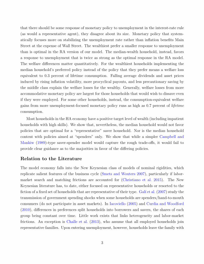
New Keynesian model with search and matching frictions, physical capital, self-insurance, and
rich household heterogeneity. We find important implications of heterogeneity for monetary
policy. This is so, even though we calibrate the model to a tranquil period (1984Q1 to 2008Q3).
We show that heterogeneity has a substantial impact on the business cycle. Relative to a
representative-agent (“RA” henceforth) counterfactual, the volatility of aggregate consumption
rises by 14 percent. The volatility of GDP rises by less, namely, 4 percent. Market incomplete-
ness means that a significant mass of households in the heterogeneous-agent (“HA”) model adjust
consumption more in response to a recessionary shock than a representative household would,
precisely with a view toward adjusting savings by less. They can do so in the aggregate be-
cause, in spite of capital adjustment costs, aggregate investment is somewhat elastic. Aggregate
investment, therefore, is less volatile in the HA model than the RA counterpart. The changes
in transmission are particularly pronounced for monetary policy shocks (shocks to the nominal
interest rate), for which the consumption response on impact doubles.
Households disagree with respect to monetary policy. We first illustrate this for a one-
time one-standard-deviation monetary shock (with a half-life of three quarters). The shock
raises the nominal interest rate by 6.25 basis points (25 basis points annualized), and leads
to a contraction in economic activity and an increase in the inequality of earnings, income,
wealth, and consumption. Markups increase but the return on capital and employed labor falls.
Overall profit income, therefore, falls more than GDP, and more than labor earnings (all in
percentage terms). Nevertheless, Main Street suffers more from the shock than Wall Street. The
wealthiest are well-insured against an unemployment spell and, by assumption, hold diversified
portfolios. They suffer the same welfare cost as the RA model would suggest. The median-
wealth households’ welfare costs are 6 times that in the RA model, however, and the wealth-
poorest households’ 12 times. For the latter, the shock results in a welfare loss equivalent to 0.12
percent of lifetime consumption. Other dimensions of heterogeneity matter as well. Unemployed
households’ welfare costs are four times those of employed households. And, conditioning on
wealth, it is the households with the highest earnings capability when employed that lose most
from the contraction because a contractionary monetary shock causes a dent in their labor income
precisely when they are productive. Some households would be willing to give up a full percentage
point of lifetime consumption to avoid the one-time monetary shock.
In light of these results, we next ask how accommodative the different households would
like monetary policy to be. Toward this end, we study the transition to a stronger response to
unemployment in the central bank’s interest-rate rule while keeping fixed the inflation and unem-
ployment targets in the rule and the response coefficient to inflation. While all households agree
2
that there should be some response of monetary policy to unemployment in the interest-rate rule
(as would a representative agent), they disagree about its size. Monetary policy that system-
atically focuses more on stabilizing the unemployment rate rather than inflation benefits Main
Street at the expense of Wall Street. The wealthiest prefer a smaller response to unemployment
than is optimal in the RA version of our model. The median-wealth household, instead, favors
a response to unemployment that is twice as strong as the optimal response in the RA model.
The welfare differences matter quantitatively. For the wealthiest households implementing the
median household’s preferred policy instead of the policy that they prefer means a welfare loss
equivalent to 0.3 percent of lifetime consumption. Falling average dividends and asset prices
induced by rising inflation volatility, more procyclical payouts, and less precautionary saving by
the middle class explain the welfare losses for the wealthy. Generally, welfare losses from more
accommodative monetary policy are largest for those households that would wish to dissave even
if they were employed. For some other households, instead, the consumption-equivalent welfare
gains from more unemployment-focused monetary policy runs as high as 0.7 percent of lifetime
consumption.
Most households in the HA economy have a positive target level of wealth (including impatient
households with high skills). We show that, nevertheless, the median household would not favor
policies that are optimal for a “representative” saver household. Nor is the median household
content with policies aimed at “spenders” only. We show that while a simpler Campbell and
Mankiw (1989)-type saver-spender model would capture the rough trade-offs, it would fail to
provide clear guidance as to the majorities in favor of the differing policies.
Relation to the Literature
The model economy falls into the New Keynesian class of models of nominal rigidities, which
replicate salient features of the business cycle (Smets and Wouters 2007), particularly if labor-
market search and matching frictions are accounted for (Christiano et al. 2015). The New
Keynesian literature has, to date, either focused on representative households or resorted to the
fiction of a fixed set of households that are representative of their type. Galı et al. (2007) study the
transmission of government spending shocks when some households are spenders/hand-to-mouth
consumers (do not participate in asset markets). In Iacoviello (2005) and Curdia and Woodford
(2010), differences in preferences split households into borrowers and savers, the shares of each
group being constant over time. Little work exists that links heterogeneity and labor-market
frictions. An exception is Challe et al. (2013), who assume that all employed households join
representative families. Upon entering unemployment, however, households leave the family with
3

their share of the family’s wealth. We, instead, do not resort to the fiction of a family.
We build on incomplete-market general equilibrium models with infinitely lived agents and
aggregate uncertainty and flexible prices. Krusell et al. (2010) and Nakajima (2012a) have
introduced search and matching frictions into the framework and explored the effects of unem-
ployment insurance. Doepke and Schneider (2006) and Meh et al. (2010), among others, focus
on the wealth redistribution associated with surprise inflation under flexible prices, and Akyol
(2004) and Erosa and Ventura (2002) on steady-state inflation. Albanesi (2007) studies the
political economy of steady-state inflation. Recently, the literature has branched out to New
Keynesian models. Werning (2015) provides analytical results that highlight the importance of
countercyclical income risk, which in our model is generated by cyclical unemployment. McKay
and Reis (2015) study the role of automatic stabilizers. They keep labor-market risk exogenous.
Similarly, Guerrieri and Lorenzoni (2011) do not have a frictional labor market. McKay et al.
(2015) study how borrowing constraints alter the efficacy of monetary forward guidance. Kaplan
et al. (2016), Bayer et al. (2015), and Luetticke (2015) study the transmission of monetary policy
shocks or other business-cycle shocks when nominal and real assets have different liquidity char-
acteristics. Auclert (2015) finds that the redistribution channel is important for the transmission
of monetary policy shocks to consumption. Our paper, instead, abstracts from a portfolio com-
position decision and from modeling nominal portfolios altogether, building on the cashless limit
of Woodford (1998). What sets the current paper apart is accounting for unemployment risk and
its endogeneity to systematic monetary policy. We believe that this is of central importance for
bringing the current generation of models to speak to the Federal Reserve’s dual mandate.
Another aspect sets the current paper apart: the solution approach. We show how to adapt
the approximate-aggregation algorithm in Krusell and Smith (1998) and Reiter (2010) to the
current setting. Solving the fully non-linear model allows us to make for welfare comparisons.
We document non-linearities in both the RA and HA variants of the model. This is in line with
the non-linearities documented by Hairault et al. (2010) and Petrosky-Nadeau et al. (2015) in
real model economies. Non-linearities are also central in den Haan et al. (2015), who entertain
a heterogeneous-agent economy with labor-market search and matching frictions and money.
Nominal wage rigidity amplifies recessions if monetary policy fails to raise the money supply
in the face of deflationary pressures. In our model, instead, we assume that monetary policy
precludes amplification by following a standard Taylor rule. We show that even within those
confines, however, monetary policy does have sizable distributional effects. Last, Ravn and Sterk
(2012) study the effect of an exogenous increase in job uncertainty in a New Keynesian model
with search and matching frictions and household heterogeneity. Next to the difference in focus,
4

they entertain a much simpler environment without aggregate savings.
The rest of the paper is organized as follows. Section 2 introduces the model. Section 3
highlights the calibration and business-cycle implications of household heterogeneity. Section 4
highlights the effects of shocks on the aggregate economy and inequality. Section 5 discusses the
welfare effects of one-time shocks and of a switch to more accommodative monetary policy. A
final section concludes.
2 Model
The model economy is characterized by uninsurable income risk as in Krusell and Smith (1998).
We follow Nakajima (2012a) and Krusell et al. (2010) and assume that the job-finding rate
of unemployed households is linked to the state of the business cycle through Mortensen and
Pissarides (1994) search and matching frictions. In equilibrium a recession will be a period
of low job-finding rates. Households face market incompleteness and borrowing constraints.
Therefore, they will be impacted differently by economic downturns, depending on their wealth
and other characteristics. In addition, we assume nominal rigidities in price setting. This means
that systematic monetary policy affects the shape of aggregate fluctuations and income risk.
2.1 States
We define the model in a recursive form. Define X as the vector of aggregate state variables at
the time of production, where X = (K,N, ζ, µ). K is the aggregate capital stock. N is aggregate
employment. ζ = (Z, ζR, ζF ) is the vector of aggregate shocks: an aggregate productivity shock,
Z, a monetary policy (interest-rate) shock, ζF , and a financial “risk premium” shock, ζF . Smets
and Wouters (2007) identify these three shocks as prominent sources of business-cycle fluctua-
tions. Households are heterogeneous and characterized by four time-varying, idiosyncratic states
(e, s, β, a). e ∈ {0, 1} denotes employment status: e = 1 means a household is employed, e = 0
means it is unemployed. While the job-loss probability will be taken as exogenous, following
Shimer (2005), the job-finding rate of unemployed workers is determined endogenously.
We seek to investigate the implications for monetary policy of household income and wealth
heterogeneity. We, therefore, have to capture key features of the wealth and income distribution
in the U.S. economy. In order to match those, we introduce household heterogeneity in time
preferences (as in Krusell and Smith 1998) and skills (as in Castaneda et al. 2003), both of which
vary stochastically over time. β ∈ B = {βL, βH} denotes the household’s time-discount factor,
where 0 < βL < βH < 1. For each household, β follows a two-state first-order Markov process
with transition matrix πB. The probability of a transition from β to β′ is given by πB(β, β′).
5

Figure 1: Timing of the model
Household earnings are governed by the employment status and a household’s skill level. Let
s ∈ S represent the skill level of a household. The skill follows an S-state first-order Markov
process that is independent of the aggregate state. Denoting the transition matrix by πS, the
probability of a transition from s to s′ is πS(s, s′). The skill transitions mean that higher-skilled
households seek to self-insure not only against business-cycle risk and the risk of job loss, but also
against a fall in earnings ability. Households would, thus, accumulate precautionary savings even
if there were no business-cycle risk. Households can save by investing in a representative mutual
fund that owns all firms in the economy. a ∈ A ⊆ R denotes the share holdings of a household.
µ(e, s, β, a) is the type distribution of households, defined as an element of a canonical Borel
σ-algebra M defined over {0, 1} × S ×B × A.
2.2 Timing
The timing is shown in Figure 1. Aggregate shocks and shocks to households’ skill levels and
time preferences are drawn at the beginning of a period and become known immediately. Denote
by µ and N the type distribution and aggregate employment, respectively, before labor-market
transitions have occurred. Let X = (K, N, ζ, µ) denote the corresponding state of the economy.
Employed households lose their jobs with exogenous probability λ. Then firms post vacancies. All
unemployed households search for jobs. Matching takes place and the aggregate state becomes
X = (K,N, ζ, µ). Thereafter, the remaining decisions are made and production takes place.
2.3 Households
Preferences are time-separable with a period utility function given by u(c) = c1−σ/(1 − σ). We
first describe the problem of a household that is employed after the employment transitions have
taken place (e = 1) and has skill level s, time preference β, and asset holdings a. The household’s
6

Bellman equation is given by
W (X, 1, s, β, a) = maxc,a′≥0
{u(c) + βE
[(1− λ+ λ f(X ′)
)W (X ′, 1, s′, β′, a′)
+λ(
1− f(X ′))W (X ′, 0, s′, β′, a′)
]}s.t. c+ pa(X)a′ =
(pa(X) + da(X)
)a+ w(X)s
(1− τ(X)
),
The household chooses consumption, c, and the number of shares it wants to carry into the
next period, a′ ≥ 0, so as to maximize expected lifetime utility subject to its budget constraint.
The household takes the job-finding rate, f(X ′), the ex-dividend price of shares, pa(X), dividends,
da(X), the wage, w(X), and the payroll tax rate, τ(X), as given. The expectation operator Eis conditional on the distribution of aggregate and individual shocks going forward (ζ ′, s′, β′).
The household takes the laws of motion of the aggregate states, X ′ = G(X) and X ′ = G(X) as
given. Next period, the household will keep its current job with exogenous probability 1− λ. If
the household loses the job, it searches for employment. Its search intensity is constant. With
probability f(X ′) the household will find a new job immediately and be employed (at a new
firm). Otherwise, the household’s employment status changes to e = 0 and the household will
go through a spell of unemployment. This happens with probability λ(1 − f(X ′)). Turning to
the budget constraint, the household uses the resources it has available for consumption, c, and
for purchasing shares that it carries into the next period, pa(X)a′. The household’s resources
(right-hand side of the budget constraint) are composed of the ex-dividend value of the shares
that the household owns at the beginning of the period, pa(X)a, dividends associated with the
shares, da(X)a, and after-tax labor income, w(X)s(1 − τ(X)). Here w(X) is the real wage per
efficiency unit and τ(X) is a proportional labor-income tax rate.
If the household is unemployed after the employment transitions have taken place, its Bellman
equation is
W (X, 0, s, β, a) = maxc,a′≥0
{u(c) + βE
[f(X ′)W (X ′, 1, s′, β′, a′)
+(
1− f(X ′))W (X ′, 0, s′, β′, a′)
]}s.t. c+ pa(X)a′ = (pa(X) + da(X)) a+ b(s).
This reflects the fact that next period the unemployed household will move into employment
with state-dependent probability f(X ′) or will otherwise remain unemployed. Instead of wage
income, the unemployed receive unemployment benefits, b(s). Benefits depend on a household’s
7

skills in order to introduce in a parsimonious way that the benefits depend on past earnings.
For future reference, denote the resulting optimal decision rules for consumption and share
holdings by c = gc(X, e, s, β, a) and a′ = ga(X, e, s, β, a), respectively.
2.4 Mutual Fund
We abstract from a portfolio choice by the individual households. Households delegate financial
management to a representative mutual fund, that is, they own all their wealth through equity
claims on the fund. There are five types of assets in the economy. Only the mutual fund trades
these: equity of producers of final goods, of intermediate goods, of capital services, and of labor
services, plus one-period nominal bonds.
Firms are owned by the mutual fund and make decisions so as to maximize their market value.
Intermediate goods firms and capital services firms face dynamic decision problems. We follow
Favilukis (2013) and assume that the mutual fund prices claims based on the asset-weighted
average of its shareholders’ period-to-period valuation. Letting uc(c) mark the marginal utility
of consumption, in shorthand notation the discount factor the funds apply is
Q(X,X ′) =
∫Ma′β
uc(c′)
uc(c)dµ′.
The online appendix provides the exact formula.2
We abstract from modeling public-sector debt or money. Instead, we use the cashless limit
assumption (Woodford, 1998) commonly used in New Keynesian models. The central bank
controls the rate of return on risk-free nominal private-sector bonds. Since prices are sticky, by
setting the nominal interest rate, the central bank influences the expected real rate of return on
the nominal bonds and, in effect, the return on all other assets in the economy. Denote by Π(X)
the gross rate of inflation. Equilibrium in the bond market requires that all assets be priced
according to the mutual fund sector’s discount factor. This, for the bond investment decision,
yields a standard Euler equation (for the mutual fund rather than a household)
1 = E[Q(X,X ′)
R(X)
Π(X ′)
],
Firms transfer their profits to the mutual fund, which, in turn, distributes profits to house-
2 Other papers do not need to specify the discount factor. In Krusell and Smith (1998) households invest directlyin capital and firms only have static rental decisions to make. In den Haan et al. (2015) there are only laborfirms. They only make one decision (to post a vacancy or not). Neither paper has sticky prices. See Carceles-Poveda and Coen-Pirani (2010) for results regarding investor unanimity with heterogeneous households.
8

holds in the form of dividends. Since we still need to introduce some notation, we report the
exact expression for dividends per share, da(X), only in equation (9) further below.
2.5 Producers of Intermediate Goods
There is a unit mass of firms that produce differentiated intermediate goods. An intermediate
good producer j ∈ [0, 1] buys labor and capital services lj and kj at the competitive rates h(X)
and r(X), respectively. The producer sells its output to final goods firms under monopolistic
competition at price Pj. In the following, let Xp := (X,µp) be state X augmented by the distri-
bution across firms of last period’s prices, Pj,−1. There are nominal rigidities: Price adjustment
is subject to Rotemberg (1982)-type quadratic adjustment costs. The producer’s value is:
JI(Xp) = maxPj ,`j ,kj
yj(X,P, Pj)
(Pj
P (Xp)
)− r(X)kj − h(X)`j − Ξ− ψ
2
(PjPj,−1
− Π
)2
y(X)
+ E [ζFQ(X,X ′)JI(X′, Pj)]
s.t. yj(X,Pj, P ) =
(Pj(Xp)
P (Xp)
)−εy(X), (1)
yj(X,Pj, P ) = Zkθj `1−θj , (2)
where yj(X,Pj, P ) is firm j’s output and y(X) is production of the final good. Constraint (1)
is the firm’s demand function, ε > 1. y(X) is the aggregate output of final goods. Equation
(2) is the production function of intermediate good j. Ξ ≥ 0 is a fixed cost of production. y
is steady-state output. Parameter ψ > 0 indexes the extent of nominal rigidities. Π takes on a
fixed value.
Letting Z be steady-state total factor productivity (TFP), TFP itself evolves according to:
log(Z ′) = (1− ρZ) log(Z) + ρZ log(Z) + εZ , where εZ is i.i.d. N(0, σ2Z), ρZ ∈ [0, 1).
The financial shock, ζF , drives a wedge between the firm’s evaluation of future profits and the
mutual fund’s. This shock, which leads to impulse responses similar to the risk-premium shock
of Smets and Wouters (2007), pertains to equity investments only. We assume that
log(ζF ) = ρζF log(ζF ) + εζF , where εζF is i.i.d. N(0, σ2ζF
), ρζF ∈ [0, 1).
If their prices last period are identical, in equilibrium all intermediate good producers will set
the same price this period as well. The optimal behavior of these firms can then be described by
9

the current aggregate rate of inflation, Π(X), and other contemporaneous aggregate variables or
the expectations of each of these. This means past prices, Pj,−1, are not state variables. Each
producer j faces the same marginal costs and chooses the same amount of labor and capital
inputs, so kj = k(X) and lj = l(X). Next, we turn to the production of these inputs.
2.6 Producers of Capital Services
There is a representative capital-producing firm, the value of which is
JK(X,K) = maxv,i,K′
{r(X)Kv − i+ E [ζFQ(X,X ′)JK(X ′, K ′)]
}(3)
s.t. K ′ =(1− δ(v)
)K + ζ
(i
K
)K. (4)
The capital-producing firm produces homogeneous “capital services.” It sells these to the in-
termediate goods sector at the competitive rate r(X). Capital services are the product of the
capital stock, K, and the utilization rate of capital, v. The rate of depreciation of capital, δ(v),
increases with utilization. The functional form follows Greenwood et al. (1988), namely,
δ(v) = δ0 vδ1 , δ0 > 0, δ1 > 1.
Capital producers decide how much to invest in next period’s capital stock, K ′. Due to capital
adjustment costs, capital investment (i) does not translate one-to-one into new capital. We
follow Jermann (1998) by specifying the functional form of these adjustment costs as
ζ
(i
K
)= ζ0
(i
K
)1−ζ1+ ζ2.
The problem of the capital-producing firm characterizes aggregate investment i(X), the aggregate
utilization rate v(X), and the aggregate capital stock next period K ′(X).
2.7 Producers of Labor Services
Labor agencies produce homogeneous “labor services.” Labor agencies may be matched with
exactly one household or they are not matched. The value of a matched labor agency is
JL(X, s) =(h(X)− w(X)
)s+ E
[ζFQ(X,X ′)(1− λ)JL(X ′, s′)
].
The labor agency produces an amount s of labor services, where s is the skill level of the household
it employs. Labor services are sold at competitive rate h(X). Wage payments are indexed by the
10
skill level. Last, the continuation value reflects the fact that only with probability (1−λ) will the
match between a labor agency and its household be producing in the next period. Otherwise,
the match will be dissolved. The exposition here anticipates that due to free entry, the value of
a labor agency not matched to a household is zero.
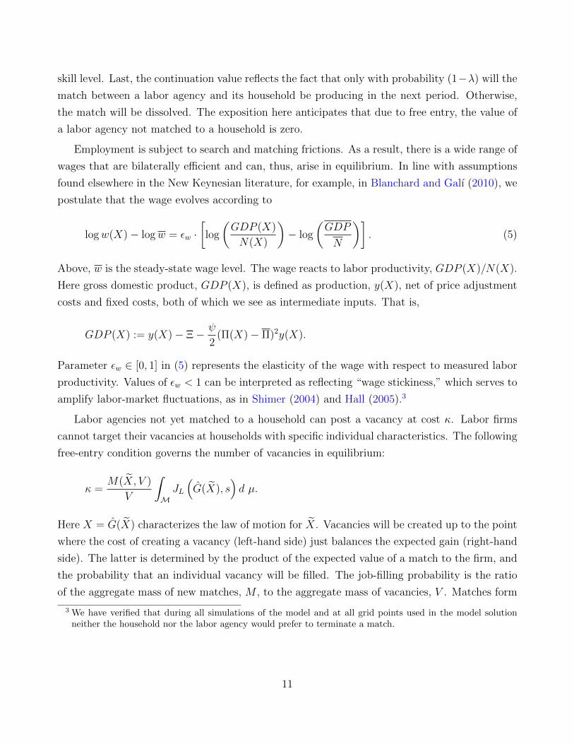
Employment is subject to search and matching frictions. As a result, there is a wide range of
wages that are bilaterally efficient and can, thus, arise in equilibrium. In line with assumptions
found elsewhere in the New Keynesian literature, for example, in Blanchard and Galı (2010), we
postulate that the wage evolves according to
logw(X)− logw = εw ·[log
(GDP (X)
N(X)
)− log
(GDP
N
)]. (5)
Above, w is the steady-state wage level. The wage reacts to labor productivity, GDP (X)/N(X).
Here gross domestic product, GDP (X), is defined as production, y(X), net of price adjustment
costs and fixed costs, both of which we see as intermediate inputs. That is,
GDP (X) := y(X)− Ξ− ψ
2(Π(X)− Π)2y(X).
Parameter εw ∈ [0, 1] in (5) represents the elasticity of the wage with respect to measured labor
productivity. Values of εw < 1 can be interpreted as reflecting “wage stickiness,” which serves to
amplify labor-market fluctuations, as in Shimer (2004) and Hall (2005).3
Labor agencies not yet matched to a household can post a vacancy at cost κ. Labor firms
cannot target their vacancies at households with specific individual characteristics. The following
free-entry condition governs the number of vacancies in equilibrium:
κ =M(X, V )
V
∫MJL
(G(X), s
)d µ.
Here X = G(X) characterizes the law of motion for X. Vacancies will be created up to the point
where the cost of creating a vacancy (left-hand side) just balances the expected gain (right-hand
side). The latter is determined by the product of the expected value of a match to the firm, and
the probability that an individual vacancy will be filled. The job-filling probability is the ratio
of the aggregate mass of new matches, M , to the aggregate mass of vacancies, V . Matches form
3 We have verified that during all simulations of the model and at all grid points used in the model solutionneither the household nor the labor agency would prefer to terminate a match.
11

according to the following matching function:
M(X, V ) =
(U(X) + λN(X)
)V((
U(X) + λN(X))α
+ (V )α) 1α
, α > 0. (6)
Here U(X) + λN(X) is the measure of households searching for a job (remember the timing
assumption discussed in Section 2.2). Matching function (6), taken from den Haan et al. (2000),
ensures that job finding and job filling rates are always well-defined probabilities. All households
without a job have the same job finding rate, namely,
f(X) =M(X, V (X))
U(X) + λN(X).
2.8 Producers of the Final Good
Final goods can be used for consuming, investing, facilitating price adjustment, and creating
vacancies. There is a representative competitive final good firm. It transforms the differentiated
intermediate goods yj, j ∈ [0, 1], into a homogeneous output good, taking the input prices Pj(Xp)
as given. The problem of the representative final good producer is
maxy,(yj)j∈[0,1]
P (Xp)y −∫ 1
0
Pj(Xp)yjdj s.t. y =
(∫ 1
0
yε−1ε
j dj
) εε−1
.
The optimal decision translates into the demand function anticipated in (1).
2.9 Central Bank and Fiscal Authority
The central bank sets the gross nominal interest rate, R, according to the following Taylor rule
log
(R(X)
RCB
)= φΠ log
(Π(X)
ΠCB
)− φu
(U(X)− U CB
)+ ζR, (7)
where U(X) = 1 − N(X) is the unemployment rate at the end of the period. All else equal,
the central bank thus raises the nominal rate above RCB
whenever inflation exceeds the inflation
target of ΠCB
(parameter φΠ > 1) and when the unemployment rate is lower than its target value
UCB
(parameter φu ≥ 0). The superscripts “CB” here signal that these are target values given
to the central bank. There are persistent monetary policy shocks, ζR, that capture deviations
12

from typical behavior, with
log(ζ ′R) = ρζR log(ζR) + εζR , where εζR is i.i.d. N(0, σ2ζR
) , ρζR ∈ [0, 1).
The fiscal authority runs a balanced-budget policy so that∫M1e=0 b(s) dµ = τ(X)
∫M1e=1 w(X)s dµ. (8)
The government pays unemployment benefits b(s) for an unemployed household of skill s (1
marks the indicator function). This is financed by a proportional tax τ(X) on the labor income
of employed households.4
2.10 Aggregate Laws of Motion
Next, we discuss how to construct the aggregate law of motion. For expositional purposes, we
use two sets of aggregate state vectors, X and X, that differ in time of measurement (at the
beginning of the period and at the end of the period, respectively); compare Section 2.2. We
therefore have three types of laws of motion, X ′ = G(X), X ′ = G(X), and X = G(X). Let us
focus on one element of X at a time.
First, installed capital K does not change during a period. It therefore does not differ between
X and X, so we only need one law of motion for K; compare equation (4):
K ′(X) =[1− δ
(v(X)
)]K + ζ
(i(X)
K
)K
where v(X) and i(X) are obtained from the optimization problem of the capital-producing sector.
Next, the law of motion for employment during the production stage of this period is given by
N(X) = (1− λ)N(X) +M(X, V (X)).
Since there are no labor-market transitions at the end of the period, employment at the beginning
of the next period coincides with employment at the end of the current period: N ′(X ′) = N(X).
Last, we need to keep track of the type distribution of households. Remember that, at the
beginning of a period, the type distribution is µ(e, s, β, a), where e is the employment status
before the separations and hiring occur. The type distribution during the period (after the
4 The proportional tax reduces the labor income of employed households, yet does not distort their labor supplydecisions (search effort is assumed to be exogenous) nor firms’ hiring decisions (because of the wage rule).
13
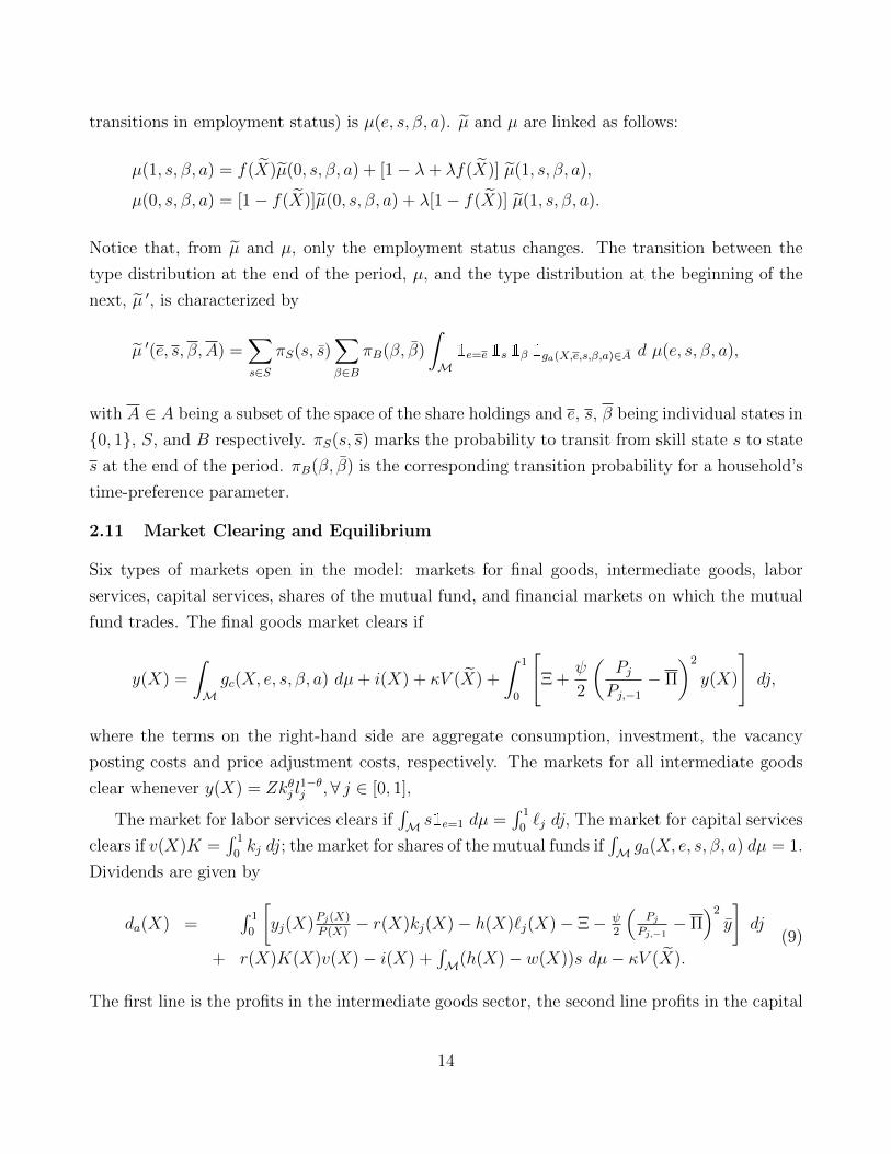
transitions in employment status) is µ(e, s, β, a). µ and µ are linked as follows:
µ(1, s, β, a) = f(X)µ(0, s, β, a) + [1− λ+ λf(X)] µ(1, s, β, a),
µ(0, s, β, a) = [1− f(X)]µ(0, s, β, a) + λ[1− f(X)] µ(1, s, β, a).
Notice that, from µ and µ, only the employment status changes. The transition between the
type distribution at the end of the period, µ, and the type distribution at the beginning of the
next, µ ′, is characterized by
µ ′(e, s, β, A) =∑s∈S
πS(s, s)∑β∈B
πB(β, β)
∫M1e=e 1s 1β 1ga(X,e,s,β,a)∈A d µ(e, s, β, a),
with A ∈ A being a subset of the space of the share holdings and e, s, β being individual states in
{0, 1}, S, and B respectively. πS(s, s) marks the probability to transit from skill state s to state
s at the end of the period. πB(β, β) is the corresponding transition probability for a household’s
time-preference parameter.
2.11 Market Clearing and Equilibrium
Six types of markets open in the model: markets for final goods, intermediate goods, labor
services, capital services, shares of the mutual fund, and financial markets on which the mutual
fund trades. The final goods market clears if
y(X) =
∫Mgc(X, e, s, β, a) dµ+ i(X) + κV (X) +
∫ 1
0
[Ξ +
ψ
2
(PjPj,−1
− Π
)2
y(X)
]dj,
where the terms on the right-hand side are aggregate consumption, investment, the vacancy
posting costs and price adjustment costs, respectively. The markets for all intermediate goods
clear whenever y(X) = Zkθj l1−θj ,∀ j ∈ [0, 1],
The market for labor services clears if∫M s1e=1 dµ =
∫ 1
0`j dj, The market for capital services
clears if v(X)K =∫ 1
0kj dj; the market for shares of the mutual funds if
∫M ga(X, e, s, β, a) dµ = 1.
Dividends are given by
da(X) =∫ 1
0
[yj(X)
Pj(X)
P (X)− r(X)kj(X)− h(X)`j(X)− Ξ− ψ
2
(Pj
Pj,−1− Π
)2
y
]dj
+ r(X)K(X)v(X)− i(X) +∫M(h(X)− w(X))s dµ− κV (X).
(9)
The first line is the profits in the intermediate goods sector, the second line profits in the capital
14

services and labor services sectors net of investment in capital and vacancies, respectively.
Last, the financial markets on which the mutual fund trades clear when all firms are held by
the mutual fund and inside bonds are in zero net supply. For a formal definition of recursive
equilibrium, see the the appendix.
3 Calibration
The model is solved numerically using a solution method that is adapted from Krusell and
Smith (1998) and Reiter (2010). Our solution algorithm, described in detail in the appendix,
takes non-linearities and uncertainty in both aggregate and idiosyncratic dynamics into account.
We calibrate the model to the U.S. economy, one period being a quarter. The calibration
sample is 1984Q1 to 2008Q3. Several parameters are set such that the steady state in the model
without aggregate shocks (“steady state” henceforth) matches long-run averages in the data.
Other parameters are set with a view toward targeting second moments in the data. The latter
set of parameters are chosen to match the second moments in the representative-agent (“RA”
henceforth) counterpart of our heterogeneous-agent model (“HA” henceforth). Given the numer-
ical burden of the solution algorithm used to solve the HA model, we do not use the simulated
method of moments to directly match the heterogeneous-agent model to long-run moments.5 In
this context, we choose the systematic response of monetary policy to unemployment (φu), the
investment adjustment cost parameter (ζ1), and the volatilities of the financial and TFP shocks
to jointly match the volatility of HP-filtered log inflation, unemployment, output, and consump-
tion. We target consumption volatility, because this is of direct relevance for welfare. Tables
1 and 2 summarize the values we choose for the calibrated parameters. We will discuss these
choices next.
3.1 Households
We set the coefficient of relative risk aversion to σ = 1.5, as, for example, in Castaneda et
al. (2003). The parameters that we calibrate next are those that pertain to the heterogeneity
in skills and time preferences. This heterogeneity allows us to match key moments related to
earnings risk and the wealth distribution. We assume that the time-preference parameter β
follows a two-state first-order Markov process with values βL and βH . Skills s follow a four-state
first-order Markov process. Time preferences and skills are independent of the business cycle.
We parameterize the time-discount factor and the skill process by ensuring that in the steady
state the model meets the following targets: (i) the Gini index of wealth is 0.81; (ii) the wealth-
5 The RA model has β = 0.99 so as to match the same steady-state real rate as in the HA model.
15

Table 1: Calibrated Parameters
Households Capital services Ξ 0.303 RCB
1.015σ 1.5 ζ0 0.721 Labor market φΠ 1.500πBβ, β
′ Table 2 ζ1 0.104 λ 0.100 φu 0.107βL 0.849 ζ2 –0.0017 α 1.716 ShocksβH 0.993 δ0 0.015 w 0.670 ρζR 0.800πSs, s
′ Table 2 δ1 1.673 εw 0.450 σζR ∗ 100 0.0625s1 0.341 Intermediate goods κ 0.249 ρζF 0.800s2 0.778 ε 3.00 Monetary policy σζF ∗ 100 0.135
s3 1.774 θ 0.231 ΠCB
1.005 ρZ 0.950s4 9.158 ψ 38.08 uCB 0.057 σZ ∗ 100 0.576
Π 1.005 Z 0.843
Notes: The table shows the calibrated parameters. The main text explains the calibration targets.
poorest 30 percent of households have a total net worth of 0; (iii) the standard deviation of
residual earnings of continuously employed workers is 0.19;6 (iv) the autocorrelation of residual
earnings of continuously-employed workers is 0.95; (v) 1 percent of the households are much
more skilled than the rest (“super-skilled,” see below); and (vi) the probability of remaining a
super-skilled worker is 0.97. Targets (i) and (ii) are derived using the 2007 Survey of Consumer
Finances. The values of targets (iii) and (iv) are taken from Krueger et al. (2015) and capture
persistent idiosyncratic shocks to earnings conditional on staying employed. Targets (v) and (vi)
are based on the discussion in Nakajima (2012b) on how to calibrate an income process with
super-skilled households.
For the time-discount factor, β, we impose two additional targets: a real rate of return of
4 percent in the steady state and we calibrate the transition matrix such that each household
redraws its discount factor on average every 40 years and has an equal chance of drawing each
of the two in this event. The idea follows Krusell and Smith (1998) and aims to capture in-
tergenerational changes in the saving behavior of dynasties. This results in values βL = 0.849
and βH = 0.993 and the transition matrix shown in the left matrix of Table 2. For the income
process we use four discrete skill levels. s1 is the lowest skill level, s2 a medium skill level, and
s3 a high skill level. The fourth skill level, s4, is used to capture vastly more productive house-
holds, the “super-skilled.” We parameterize the skill transitions as follows. Skill transitions are
independent of the business cycle (and of employment). The process of transitions between the
lower three skill levels is assumed to be governed by a discretized AR(1) process for the log of
6 The value is taken from Krueger et al. (2015), who estimate an AR(1) process for residual labor earnings afterremoving age, education, and time effects.
16

Table 2: Transition Probabilities
Time-discount factor, πB(β, β′) Skills, πS(s, s′)
tomorrow tomorrowβL βH s1 s2 s3 s4
today βL 0.9969 0.0031
today
s1 0.9463 0.0528 0.0007 0.0002
βH 0.0031 0.9969 s2 0.0264 0.9470 0.0264 0.0002
s3 0.0007 0.0528 0.9463 0.0002
s4 0.0069 0.0069 0.0069 0.9793
Notes: Transition probabilities per quarter. Left: πB(β, β′). Right matrix: πS(s, s′). s1 : lowest skillgroup, s4 : highest skill group. Rounding for the table means rows may not sum to 1.
individual productivity with mean zero, persistence ρs and variance of the innovation σ2s . We
discretize using the algorithm described in Rouwenhorst (1995). For the transitions to or from
the super-skilled state, we assume that the probability of becoming super-skilled is the same for
each normal skill level. Similarly, a household that loses its super skills is equally likely to transi-
tion into either of the three “normal” skill levels. With these assumptions, there are three sets of
parameters associated with the super-skilled state: the probability of staying super-skilled, πs4,s4 ,
the probability that a “normal” household becomes super-skilled, πs1,s4 = πs2,s4 = πs3,s4 , and the
productivity of the super-skilled, s4. Table 2 reports the resulting transition probabilities per
quarter.
Figure 12 in the appendix shows that the calibrated model closely matches the wealth distri-
bution in the U.S. economy. In the same appendix, Table 6 shows that the model matches the
main feature originating from this observation, namely, that “Wall Street” (the 5 percent wealth-
iest households) derive a large share of income from financial wealth, whereas “Main Street” (the
remaining 95 percent) does not.
3.2 Producers of Capital Services
We set the curvature parameter of capital adjustment costs to ζ1 = 0.104. We require the steady
state with adjustment costs to be the same as the one without such costs. This determines the
remaining parameters for capital adjustment. The resulting values are shown under “Capital
services” in Table 1. Furthermore, we require that the utilization rate of capital be unity in the
steady state and that the steady-state depreciation rate be 6 percent per year. This pins down
parameters δ0 and δ1.
17
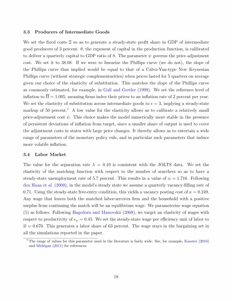
3.3 Producers of Intermediate Goods
We set the fixed costs Ξ so as to generate a steady-state profit share in GDP of intermediate
good producers of 3 percent. θ, the exponent of capital in the production function, is calibrated
to deliver a quarterly capital to GDP ratio of 8. The parameter ψ governs the price adjustment
cost. We set it to 38.08. If we were to linearize the Phillips curve (we do not), the slope of
the Phillips curve thus implied would be equal to that of a Calvo-Yun-type New Keynesian
Phillips curve (without strategic complementarities) when prices lasted for 5 quarters on average
given our choice of the elasticity of substitution. This matches the slope of the Phillips curve
as commonly estimated, for example, in Galı and Gertler (1999). We set the reference level of
inflation to Π = 1.005, meaning firms index their prices to an inflation rate of 2 percent per year.
We set the elasticity of substitution across intermediate goods to ε = 3, implying a steady-state
markup of 50 percent.7 A low value for the elasticity allows us to calibrate a relatively small
price-adjustment cost ψ. This choice makes the model numerically more stable in the presence
of persistent deviations of inflation from target, since a smaller share of output is used to cover
the adjustment costs in states with large price changes. It thereby allows us to entertain a wide
range of parameters of the monetary policy rule, and in particular such parameters that induce
more volatile inflation.
3.4 Labor Market
The value for the separation rate λ = 0.10 is consistent with the JOLTS data. We set the
elasticity of the matching function with respect to the number of searchers so as to have a
steady-state unemployment rate of 5.7 percent. This results in a value of α = 1.716. Following
den Haan et al. (2000), in the model’s steady state we assume a quarterly vacancy-filling rate of
0.71. Using the steady-state free-entry condition, this yields a vacancy posting cost of κ = 0.249.
Any wage that leaves both the matched labor-services firm and the household with a positive
surplus from continuing the match will be an equilibrium wage. We parameterize wage equation
(5) as follows. Following Hagedorn and Manovskii (2008), we target an elasticity of wages with
respect to productivity of εw = 0.45. We set the steady-state wage per efficiency unit of labor to
w = 0.670. This generates a labor share of 63 percent. The wage stays in the bargaining set in
all the simulations reported in the paper.
7 The range of values for this parameter used in the literature is fairly wide. See, for example, Kuester (2010)and Midrigan (2011) for references.
18

3.5 Central Bank
The inflation target (ΠCB
) is set such that the model implies a steady-state inflation rate of 2
percent annualized, in line with the Federal Reserve System’s inflation objective. The rate RCB
used in the Taylor rule (7) is chosen to deliver a target for the steady-state real rate of return of
4 percent. The response of the policy rate to inflation in the Taylor rule is set at φΠ = 1.5 as in
Taylor (1993). The response parameter to unemployment is set to φu = 0.107. The target level
for the unemployment rate, UCB
, is set to the steady-state level of unemployment (0.057).
3.6 Fiscal Authority
The unemployment benefit system mimics the system in place in the U.S. in that the replacement
rate is assumed to be 40 percent of the steady-state wage (as in Shimer 2005) for the lower skill
groups. Benefits are capped at 40 percent of the mean earnings in the economy. That is,
b(s) = min(b · s · w, b · economy-wide average earnings in steady state). The payroll tax rate is
set so as to balance the budget on a period-by-period basis. The choices above imply a steady-
state payroll tax rate of 2.42 percent.
3.7 Shocks
The steady-state level of the TFP shock, Z, is chosen so as to normalize steady-state GDP to
unity. The persistence of the TFP shock is ρZ = 0.95. The standard deviation of the TFP shock
(σZ = 0.0058) was calibrated such that GDP in the RA version of the model (once HP-filtered)
has the same standard deviation as HP-filtered GDP in the data. The persistence of the monetary
policy shock, ρD = 0.8, was chosen so as to have persistence of the real rate after a monetary
policy shock. Its standard deviation, σD, is calibrated to 0.000625, so that the annualized size of
a typical monetary policy shock is 6.25 basis points (25 basis points annualized), the typical size
of monetary policy shocks in VAR studies over our calibration sample. See, for example, Altig et
al. (2011). Finally, we calibrate the financial shock to have the same persistence as the monetary
policy shock, and a standard deviation such that the model meets the volatility targets specified
at the beginning of this section.
3.8 Business-Cycle Statistics
In this section we show that the calibrated model matches the business-cycle facts well. In
addition, we show that household heterogeneity changes the business cycle. In the HA model
consumption is almost 15 percent more volatile than in the RA counterpart. At the same time
investment is 10 percent less volatile. GDP on net is 4 percent more volatile in the HA model
19

than in the RA counterpart.
Table 3 compares second moments implied by the model and the data (based on HP-filtered
series with smoothing parameter 1,600). The data are described in the appendix. The first
Table 3: Model vs. Data – Second Moments
Model Data
HA: heterog. hh. RA: represent. hh. 1984Q1-2008Q3
Std Corr AR(1) Std Corr AR(1) Std Corr AR(1)
Output and components
GDP (GDP ) 1.69 1.00 0.63 1.62 1.00 0.64 1.62 1.00 0.94
Consumption (c) 1.02 0.99 0.69 0.89 0.98 0.71 0.89 0.87 0.87
Investment (i) 5.28 0.98 0.73 5.86 0.99 0.71 5.09 0.96 0.89
Capacity utilization (v) 0.96 0.78 0.24 0.83 0.75 0.27 2.21 0.84 0.94
Labor market
Employment N(X) 0.65 0.90 0.64 0.62 0.90 0.66 0.65 0.86 0.96
Unemployment U(X) 10.9 -0.90 0.65 10.2 -0.89 0.67 10.2 -0.86 0.95
Vacancies (V ) 8.94 0.75 0.07 8.35 0.73 0.10 11.1 0.91 0.93
Job finding rate (f) 5.37 0.88 0.38 5.08 0.87 0.40 5.13 0.80 0.83
Productivity and Prices
GDP (X)/N(X) 1.14 0.97 0.62 1.10 0.97 0.63 1.07 0.87 0.88
Wage W (X) 0.51 0.97 0.62 0.50 0.97 0.63 0.95 0.41 0.84
Inflation Π [1] 0.67 -0.32 0.62 0.67 -0.40 0.63 0.67 0.27 0.27
Nominal rate R [1] 0.97 -0.14 0.58 0.96 -0.25 0.60 1.24 0.61 0.92
Notes: The table compares moments of the data and two variants of the model (heterogeneous households,representative households). The model moments are based on 1,000 repeated simulations of the model. Eachsimulation is initialized with 500 periods of simulations that are dropped for the computation of the moments.The next 139 periods are kept. In each case, we take the natural log of the data and compute the cyclicalcomponent of the data multiplied by 100 so as to have percentage deviations from trend. The trend is an H-P-trend with weight 1,600. We then drop the first 20 and last 20 observations and compute moments of interest.Finally, we average across the simulations. The left block shows the model’s moments, the block on the rightthe data’s. The first column (“Std.”) reports the standard deviation of each series. The second column(“Corr”) shows the correlation of the series with GDP. The final column (“AR(1)”) shows the autocorrelationof the series. [1]: the nominal interest rate and inflation are reported in annualized percentage points.
three columns report second moments in the baseline model with heterogeneous agents (the HA
model). The second block of three columns reports the second moments of the representative-
agent version of the model (the RA model). These moments are included here for two reasons.
First, because we use the RA model to calibrate the model to second moments in the data.
Second, it shows how much the heterogeneity influences aggregate fluctuations. The final set of
columns reports the moments in the data. The model fits the data well. The model also generates
an increase in the skewness of earnings growth in recessions (not reported in the table). Namely,
20

the average correlation of year-on-year GDP growth and the skewness of yearly earnings growth
is 0.14. Still, the value falls short of the value of 0.5 reported for the same statistic in Guvenen
et al. (2014).
A result of economic substance is that allowing for heterogeneity implies notable changes to
the business cycle. The model with heterogeneous households generates much more volatility
in aggregate consumption than we observe under representative households. It is important to
bear in mind, however, that households in the model can save and that the supply of aggregate
savings (capital and employment relationships) is endogenous to their desire to save. Therefore,
the higher volatility of consumption does not translate one-to-one into more volatile aggregate
demand. Rather, the volatility of output rises only by 4 percent. The reason is that the volatility
of investment falls by 11 percent relative to the RA environment. Table 7 in the appendix shows
that simple saver-spender models (introduced in more detail in Section 5.2) capture the change
in business-cycle dynamics only if calibrated to a large share of spenders.
The sections that follow have two purposes. First, in Section 4 will we contrast the trans-
mission of shocks in the HA model and the RA variant, conditional on the baseline calibration
of the Taylor rule φπ = 1.5, φu = 0.107. This will illustrate, in particular, the reasons for the
change in the business cycle stressed above. Thereafter, in Section 5, we will discuss the welfare
implications both of monetary policy shocks and of the design of the monetary rule.
4 Transmission of TFP and Monetary Policy Shocks
Next, we discuss in detail how heterogeneity affects the transmission of shocks. The central
result is: Allowing for household heterogeneity changes the transmission of shocks, in particular
monetary policy shocks. For these, the consumption response on impact is about twice as large
in the HA model as in the RA model. The impact response of GDP is larger as well, but less so
than for consumption. We argue that this owes to the interaction of the precautionary savings
motive with the endogeneity of aggregate investment in the HA model.
4.1 Transmission of a Technology Shock
We first discuss the response of the economy to a TFP shock. This shock is the main driver of
the business cycle in the model. The starting point is the “stochastic steady state.”8 Figure 2
shows the effect of a one-standard-deviation positive TFP shock for the aggregate economy. The
solid lines show the response in the baseline model (the model with heterogeneous households).
8 The stochastic steady state is defined as follows. We initialize the economy at the non-stochastic steadystate. Then we simulate 500 periods of the stochastic economy, assuming that in each period unexpectedlythe innovations to the three shocks are zero. The resulting state in period 500 is the “stochastic steady state.”
21

The dashed lines show the response in the model with a representative household. Output
Figure 2: Response to a TFP Shock I
GDP Consumption Investment
0 5 10 15 200.6
0.8
1
1.2
per
cen
t
heterog.represent.
0 5 10 15 200.5
0.6
0.7
per
cen
t
0 5 10 15 20
1.52
2.53
3.5
per
cen
t
Unemployment Rate Job Finding Rate Wage
0 5 10 15 20−0.3
−0.25
−0.2
pp.
0 5 10 15 20
1
1.5
2p
p.
0 5 10 15 200.2
0.3
0.4
per
cen
t
heterog.represent.
quarters quarters quarters
Notes: Impulse response to a one-standard-deviation TFP shock, Z. Solid line: the model economy with hetero-geneous households. Dashed line: same economy but with a representative household. For most of the variables,the y axis shows percent deviations from the no-shock path (y-label “percent”). “pp.” refers to the deviationfrom the no-shock path in percentage points. The x-axis shows time since the shock in quarters.
rises in response to the TFP shock in response to the TFP shock and the demand for labor
services increases. Labor services firms, therefore, post more vacancies. The job-finding rate
rises markedly, by about 2 percentage points on impact. The unemployment rate falls, namely,
by about 0.3 percentage point. The wage rises.9
What differs strongly is the composition of the increase in output. The HA model’s con-
sumption rises about 15 percent more, whereas its investment response is weaker than the RA
model’s. We turn to explaining these differences next.
Toward this end, Figure 14 in the appendix shows the steady-state savings policies for each
type of household types. From this it is apparent that unemployed households generally dissave,
at a rate that increases in wealth. Employed households are more complicated. Employed
households of the patient type (βH) have a positive target level of wealth, even if – for the low-
skilled (s1) – this may be just about one-tenth of annual income. Employed households that
are impatient (βL) will accumulate savings only if they are in one of the higher skill groups
9 The response of (un)employment is consistent with the responses to permanent TFP shocks identified by Ravnand Simonelli (2008) and Altig et al. (2011) by means of long-run restrictions, and the responses identified bysign restrictions to persistent but possibly transitory TFP shocks in Dedola and Neri (2007).
22

(s3 and s4). The TFP shock affects employment, unemployment risk, and income. On the one
hand, it moves more households from unemployment to employment. For some households, the
additional income will translate one-to-one into additional consumption, making consumption
more volatile than in the RA model. This effect alone would be present in a simple saver-spender
model of the business cycle as well. What is more, however, is that there are households who
have some savings but risk hitting the borrowing constraint during an extended unemployment
spell. The positive TFP shock leads these households to reduce their precautionary savings.
They do so by selling shares and by influencing the investment policy of capital-services firms
(as implicitly embedded in their influence on the stochastic discount factor), namely, in such
a way that investment rises by less than in the RA model. Figure 3 shows the counterpart to
this, the individual HA model household’s consumption response on impact depending on the
Figure 3: Consumption Response to a TFP shock
Notes: Consumption response (on impact) to a one-standard-deviation positive TFP shock by householdtype (β, e, a, s). For each decile of the wealth distribution, skills are ordered from lowest to highest (“s1” to“s4”). No bar means that, for that type, consumption on impact does not respond to the TFP shock. y-axis:percentage increase in consumption relative to no-shock baseline. For comparison, the dashed horizontal linereports the impact response in the RA model.
household’s wealth, its time-preferences, skills, and employment status. For comparison, the
23
horizontal dashed line shows the response in the RA model. The figure suggests that it is the
unemployed, in particular, who adjust their consumption, as long as they hold wealth.10 These
households’ future unemployment risk has fallen (since the job-finding rate rises persistently),
rendering saving less important. In addition, the value of their shares has risen. This increases
the scope for consuming out of wealth during any unemployment spell.
In sum, the consumption response alone would suggest that GDP in the HA model reacts
very differently from the RA counterpart. The actual impact response of GDP differs only by
four percent between the two variants, however. The key to understanding this is that part of
the mirror image of the stronger response of consumption to a TFP shock is that investment in
the HA model does not rise by as much as in the RA counterpart. The compensating weaker
response of investment shows the importance of modeling an economy in which aggregate saving
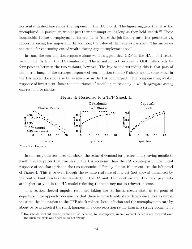
can respond to shocks.
Figure 4: Response to a TFP Shock II
Dividends Capital
Share Price per Share Stock
0 5 10 15 200.85
0.90.95
11.05
per
cen
t
heterog.represent.
0 5 10 15 200.5
0.6
0.7
0.8
per
cen
t
0 5 10 15 20
0.2
0.4
0.6
per
cen
t
quarters quarters quarters
Notes: See Figure 2.
In the early quarters after the shock, the reduced demand for precautionary saving manifests
itself in share prices that rise less in the HA economy than the RA counterpart. The initial
response of the share price in the two economies differs by almost 10 percent; see the left panel
of Figure 4. This is so even though the ex-ante real rate of interest (not shown) influenced by
the central bank reacts rather similarly in the RA and HA model variant. Dividend payments
are higher early on in the HA model reflecting the tendency not to reinvest income.
This section showed impulse responses taking the stochastic steady state as its point of
departure. The appendix documents that there is considerable state dependence. For example,
the same-size innovation to the TFP shock reduces both inflation and the unemployment rate by
about twice as much if the shock happens in a deep recession rather than in a strong boom. This
10 Households without wealth cannot do so because, by assumption, unemployment benefits are constant overthe business cycle and there is no borrowing.
24

state dependence is already present in the RA model and allowing for household heterogeneity
amplifies the dependence only slightly.
4.2 Transmission of a Monetary Policy Shock
Next, we analyze the effect of a contractionary one-standard-deviation monetary shock. For the
purpose of the current paper, the main difference to the TFP shock will be the distributional
implications.11
4.2.1 Response of the Aggregate Economy to a Monetary Policy Shock
Figure 5 shows the response of the economy to a 25-basis-point (annualized) monetary tightening.
That is, a one-standard-deviation monetary shock. By design, the monetary policy shock is
persistent. It therefore raises the expected long-term real rate of interest. Higher expected
returns lead households to save more and cut back their spending for consumption by 0.13
percent (second panel in Figure 5). Since nominal prices are rigid, the ensuing fall in aggregate
demand is met by an increase in intermediate goods firms’ markups, validating the fall in activity.
Firms invest less in light of the rising opportunity cost and falling demand. At the same time,
capacity utilization falls. GDP overall falls by 0.3 percent. A monetary policy tightening strongly
Figure 5: Response to a Monetary Shock I
GDP Consumption Investment
0 5 10 15 20−0.3
−0.2
−0.1
0
perc
ent
heterog.represent.
0 5 10 15 20
−0.1
−0.05
0
perc
ent
0 5 10 15 20−0.8
−0.6
−0.4
−0.2
0
perc
ent
Unemployment Rate Job Finding Rate Wage
0 5 10 15 200
0.05
0.1
0.15
pp
.
0 5 10 15 20
−1
−0.5
0
pp.
0 5 10 15 20
−0.04
−0.02
0
perc
ent
heterog.represent.
quarters quarters quarters
Notes: Impulse response to a one-standard-deviation monetary policy shock, D. For further details, see the notesto Figure 2.
11 The effects of a risk shock are very similar to the monetary policy shock, so we omit them here.
25

affects the labor market (second row): On the one hand, the tightening reduces the demand for
labor services and their price. On the other hand, such a monetary policy raises the real rate
of interest and therefore makes firms discount the future by more. This further exacerbates the
fall in hiring. Along with vacancy posting, the job-finding rate falls markedly (by 1.2 percentage
points). As employment falls, the unemployment rate rises by 0.18 percentage point (from
a steady-state value of 6 percent to 6.18 percent). The reduced demand for production factors
causes a reduction in capacity utilization and output per employed household. Consequently, the
wage falls. In the model with borrowing-constrained households, this increase in unemployment
and idiosyncratic risk tends to further exacerbate the fall in consumption (second panel, first row
of Figure 5). However, it also ensures that investment and the share price do not fall as much as
in the representative agent counterpart (third panel, first row of Figure 5 and first panel Figure
6). As the discount rate rises and investment becomes less profitable, the mutual fund pays out
Figure 6: Response to a Monetary Shock II
Dividends Capital
Share Price per Share Stock
0 5 10 15 20
−0.1
−0.05
0
perc
ent
heterog.represent.
0 5 10 15 200
0.1
0.2
0.3
per
cen
t
0 5 10 15 20
−0.04
−0.02
0
perc
ent
quarters quarters quarters
Notes: See Figure 5.
free cash flow through dividends.12 Only in the medium term do dividends fall below their level
absent the monetary shock, reflecting that below-average investment in both labor and capital
drains the productive resources available to firms. Note that while dividends rise in response to
a monetary shock, this does not imply that the same is due for profits.
Importantly, the model has two different sources of ex-post profits. The left panel of Figure
7 shows that profits in the intermediate goods (sticky-price) sector rise with tighter monetary
policy, because a monetary contraction reduces marginal costs. Due to sticky prices, then,
markups in the intermediate goods sector increase. This alone would suggest that wealthier
12 Firms cannot retain earnings. This affects income accounting, but should not affect our results regardingconsumption inequality and welfare. The timing of dividends matters primarily for households that are at theborrowing constraint. These households, however, do not hold shares in the first place. All other householdscan undo dividend payments that they consider ill-timed by adjusting the number of shares they hold.
26

households stand to benefit from contractionary monetary policy. However, such an argument
neglects the fact that capital and labor services firms can make profits and/or losses ex post as
well. And since both employment and capital are investment goods in our model, the losses
that these types of firms incur after a monetary contraction can be steep. Both the rental
rate of capital r(X) and the rental rate for labor services h(X) fall (not shown). On balance,
the profits of all three types of firms (labor, capital, intermediate goods) combined fall after a
contractionary monetary policy shock, and a little more so than GDP; compare the right panel
of Figure 7. In other words, for assessing the distributional effects of monetary it is central to
Figure 7: Response to a Monetary Shock III
Intermediate goods sector Economy-wide
0 5 10 15 200
1
2
per
cen
t
0 5 10 15 20−0.4
−0.2
0
perc
ent
heterog.represent.
quarters quarters
Notes: Same as Figure 5. Shown is the response of profits in the intermediate goods sector (left panel). Andprofits in the overall economy (before physical investment and vacancy posting costs).
allow for investment opportunities other than sticky-price firms.
Lower rental rates for both labor and capital services mean lower marginal costs. Inflation
therefore falls by 0.2 percentage point (annualized); see left panel in Figure 8. By the logic of the
Taylor rule, equation (7), a positive monetary shock leads to a persistent increase in the ex ante
long-term real rate of interest. In the simulations shown here, the increase in the long-term real
rate of interest reduces inflation and unemployment in a front-loaded manner. What matters for
the contractionary effect of monetary policy is that the central bank commits to keeping the real
rate of interest higher than usual.
4.2.2 The Effect of a Monetary Shock on Inequality
Figure 9 shows the responses of the Gini indexes for earnings, income, wealth, and consumption
to a monetary shock. What is notable here is that shocks that tighten monetary policy raise
inequality in the economy. This is consistent with the empirical findings of, for example, Coibion
et al. (2012). The effects are of a magnitude similar to a TFP shock (not shown), even though
GDP falls four times more after a contractionary TFP shock, but generally less persistent.
27

Figure 8: Response to a Monetary Shock IV
Inflation Rate Nom. Interest Rate Tax Rate
0 5 10 15 20−0.2
−0.1
0
pp. (
ann.
)
0 5 10 15 20
−0.1
−0.05
0
pp. (
ann.
)
0 5 10 15 200
0.02
0.04
0.06
0.08
pp
.
quarters quarters quarters
Notes: See Figure 5.
Figure 9: Response to a Monetary Shock: Gini Indexes
Gini Earnings Gini Income Gini Wealth Gini Consumption
0 5 10 15 200
0.05
0.1
pp
.
0 5 10 15 200
0.02
0.04
pp
.
0 5 10 15 200
1
2
x 10−3
pp.
0 5 10 15 200
0.01
0.02
0.03
pp
.
quarters quarters quarters quarters
Notes: Impulse responses of Gini indexes of earnings (not conditioning on being employed), income, wealth, andconsumption to a one-standard-deviation monetary policy shock, D. The figures show percentage point increases(an increase of “1” on the y-axis would increase the earnings Gini from, say, 0.64 to 0.65).
5 Heterogeneous Welfare Effects
Next, we look at the welfare consequences of monetary policy. Section 5.1 explores the welfare
effects of one-time shocks. While negligible in a representative-agent setting, the welfare costs
of a contractionary monetary shock are notable when accounting for heterogeneity. They are
an order of magnitude larger for the wealth-poor than for the wealth-rich, and roughly four
times larger for the unemployed than the employed. Section 5.2 explores the importance of the
systematic response of monetary policy to unemployment. A vast majority of the population
favors a much stronger response to unemployment than that embedded in the baseline.
5.1 Welfare Effects of One-Time Shocks
Table 4 summarizes the welfare effects of one-time one-standard-deviation shocks. The welfare
gains (positive) or costs (negative) are measured as lifetime consumption equivalents. For ex-
ample, the entry of “0.47” in row “Top 0.1 percent” and column “TFP” means that the 0.1
percent wealthiest households on average would be willing to permanently pay 0.47 percent of
28

Table 4: Welfare Effects of One-Time Positive Shocks
One-standard-deviation shock
TFP Monetary Financial
RA, repres. agent 0.26 -0.01 -0.02
HA, household avg. 0.44 -0.07 -0.12——Top 0.1 percent 0.47 -0.01 -0.02
Top 5 percent 0.41 -0.01 -0.02
80th–95th percentile 0.34 -0.01 -0.03
60th–80th 0.29 -0.02 -0.03
40th–60th 0.41 -0.06 -0.11
30th–40th 0.54 -0.10 -0.20
By
Wea
lth
Bottom 30 percent 0.60 -0.12 -0.24
Notes: Lifetime consumption equivalent welfare gains from a one-time one-standard-deviation positiveTFP, monetary policy, and financial shock, respectively. Row “RA” reports consumption equivalentsfor a representative household. Row “HA” shows the average consumption equivalent in the population(using population weights).
their consumption to experience a positive one-standard-deviation aggregate TFP shock today.
The welfare gains are largest for the wealth-poorest 30 percent of the population, 0.60 percent.
The average consumption equivalent across all households (row, “HA”) is 0.44 percent. The
wealth-poor are at or very close to their borrowing constraint and thus benefit most from the
shock. In addition, they tend to be more impatient. The “upper middle class” gains least. On
the one hand these households are far from their borrowing constraint. In addition, they rely
mostly on labor income rather than financial income. Wage rigidity, however, imparts more of
the TFP gains to capital owners than workers and, thus, to the wealthiest segment of the pop-
ulation. Indeed, at 0.29 percent of lifetime consumption, households around the 70th percentile
of wealth gain about as much as would a representative household (compare row “RA”).
The monetary shock would have very small welfare costs if financial markets were complete
(0.01 percent of lifetime consumption, see row “RA” and the second column of Table 4), because
the way we calibrated it, the shock is rather small: it raises the nominal rate temporarily by
6.25 basis points above the level prescribed by the Taylor rule (0.25 percentage point when
annualized). The small size notwithstanding, if markets are incomplete, the monetary shock has
sizable distributional consequences. The wealth-poor on average are willing to pay as much as
0.12 percentage point of lifetime consumption to avoid this monetary shock, that is, more than
ten times as much as the RA model suggests. The less wealth a household holds, the more its
consumption will be affected by the increase in unemployment and unemployment risk and the
29

fall in the wage that the monetary tightening brings about. For the upper middle class and the
wealthiest households, instead, the monetary shock carries welfare costs about as small as those
under complete markets.13
Figure 10: Welfare Effects of a Contractionary Monetary Shock by Type
Notes: Consumption-equivalent welfare gains (negative entries mean welfare losses) by household type (β, e, a,s). For each decile of the wealth distribution, skills are ordered from lowest to highest (“s1” to “s4”). No bar isshown for those types that do not have any mass in the population.
Wealth, of course, is only one of the characteristics of a household. Figure 10 looks at the
welfare costs of a monetary shock in more detail. Each of the four panels in Figure 10 focuses on
one specific combination of time preferences (β) and employment status. In each panel, the x-axis
reports a household’s wealth level by decile of the wealth distribution. For each wealth-decile,
four bars (dark blue, light blue, green, yellow; from left to right) mark the skill of the household.
No bar is shown if the mass of households with that combination is zero. The corresponding
mass of the respective groups in the population is reported in Figure 13 in the appendix. The
y-axis shows the consumption equivalents.
Several observations are in order. First, as discussed above, lower wealth is associated with
13 The financial shock, by construction, affects the economy through the same channels as the monetary policyshock. The size of the financial shock is larger, though.
30

higher welfare costs of a monetary shock. Second, and importantly, controlling for wealth, the
skill level, and time preferences, the unemployed households are much more negatively affected by
an unanticipated monetary tightening than employed households. For example, an unemployed
low-beta low-wealth household of high skills (s3) would be willing to forgo 0.45 percent of lifetime
consumption to avoid what appears to be a rather small one-time monetary shock; see the green
bars (the respective third bars from the left) for wealth deciles 1-3 and 4 in the bottom-left panel
of Figure 10. On average, unemployed households’ welfare costs are about three times larger
than employed households’ because a monetary shock tends to prolong the unemployment spell
of an individual household. This means that lifetime earnings fall and the risk of exhausting
savings rises.
Third, and conditioning on all other characteristics, more impatient (low beta) households
are affected more negatively by a monetary shock. Conditional on wealth, their higher preference
for current consumption means that their welfare is hit particularly hard by a shock that reduces
income today and which they will not smooth over time (since the market rate of return is lower
than their rate of time preference).
Fourth, and surprisingly perhaps, all else equal the more productive a household is (the
higher the skill level s) the more a household loses from a monetary contraction. A monetary
shock means that labor earnings fall and labor-earnings risk rises for all households. What
drives the welfare losses for the high-skilled is that a monetary shock causes them to lose income
precisely when they are more productive than usual (idiosyncratic productivity s is persistent
but temporary). Therefore, unemployed super-skilled households at the 50th and 60th percentile
of the wealth distribution, for example, would be willing to pay as much as, respectively, 0.8 and
0.5 percent of lifetime consumption to forgo the shock. For aggregate welfare, however, these
households matter little since only about 0.04 percent of households have these characteristics
(Figure 13 in the appendix).
5.2 Welfare Effects of a Transition to More Accommodative Monetary Policy
So far, we took the monetary policy rule as given. In this section, we consider the welfare effects
of changes to the systematic response of monetary policy to unemployment. This response
is important because counter-cyclical monetary policy can stabilize unemployment. Not only
does this help insure households against having to run down their savings during a persistent
unemployment spell, it may also reduce the average unemployment rate itself. We compare the
policy implications of our heterogeneous-agent (HA) model with the representative-agent (RA)
counterpart and a Campbell and Mankiw (1989)-type saver-spender model (SP). Variants of the
31
latter have been used in New Keynesian models without equilibrium unemployment by Galı et al.
(2007) and Iacoviello (2005). In our SP model, some households are assumed to be “spenders,”
who consume their entire income. The difference to our model is that households choose if they
want to save or not. The central finding of this section is that a large majority of households in
the HA model are in favor of a response to unemployment that is twice as strong as would be
optimal in the RA model. The SP model provides incomplete guidance only.
The question we ask is: “Would a certain household prefer to live in the baseline economy or
have monetary policy change to being more or less responsive to unemployment?” Toward this
end we look at a one-time unanticipated change in the interest-rate response to unemployment,
φu, while keeping the response to inflation fixed at φπ = 1.5. We also keep the target levels for
inflation and unemployment in the rule constant. The initial state is the stochastic steady state
in the baseline. Welfare is assessed taking transition effects into account.
For the RA model, the optimal unemployment response is φu = 0.46. At this value, unem-
ployment fluctuates about 41 percent less than in the baseline, while inflation volatility rises by
71 percent. The reason why price stability is not optimal is that the condition is violated (Hosios,
1990) in two ways: first, wages on average are too high from a social perspective (they remain
in the bargaining set, however, and so are privately efficient) and, second, there is wage rigidity.
Blanchard and Galı (2010) and Ravenna and Walsh (2012) show this in smaller representative-
agent model economies.
Turning to the HA model, the welfare effects of switching to more “dovish” or more “hawk-
ish” monetary policy are presented in Table 5. The left-most column reports on more hawkish
policy, the four columns on the right on more dovish policy. The second-to-last row of the table
reports the share of households that would be in favor of abandoning the baseline policy rule for
a rule with an alternative value of φu. In line with the results in the RA model, all households
dislike switching to a more hawkish monetary policy (φu = 0.05). Indeed, under this policy un-
employment volatility would rise by 15 percent. Households with positive target levels of wealth
(which includes patient households and higher-skilled impatient households) respond to this by
accumulating further savings, which hurts their consumption. It is the wealthiest households
that dislike moving to a more hawkish policy most. The wealth-poor instead are partially com-
pensated for the increase in unemployment risk through the higher wages that come with more
capital (and, thus, higher labor productivity).
The last four columns of the table show the welfare gains (compared to the baseline) from
moving to more accommodative policy. In line with the exercises for the RA model, almost all
households (99.7 percent) are in favor of moving to φu = 0.25 (second-to-last row in column
32

Table 5: Welfare Effect of Permanent Policy Change
φu 0.05 0.107 0.25 0.5 0.75 1.0
RA, repres. agent -0.09 — 0.09 0.12 0.09 0.05
HA, household avg. -0.09 — 0.08 0.13 0.13 0.12——Top 0.1 percent -0.14 — 0.07 0.02 -0.10 -0.23
Top 5 percent -0.13 — 0.08 0.06 -0.03 -0.14
80th–95th percentile -0.12 — 0.08 0.09 0.04 -0.02
60th–80th -0.11 — 0.09 0.13 0.11 0.08
40th–60th -0.09 — 0.09 0.16 0.18 0.18
30th–40th -0.07 — 0.08 0.15 0.18 0.19
By
Wea
lth
Bottom 30 percent -0.07 — 0.07 0.14 0.17 0.18——Percent in favor ...
... relative to baseline 0.0 — 99.7 99.7 94 84
... relative to next-lower — 100 99.7 92.5 60 48
Notes: Welfare effects of a permanent policy change from φu = 0.107 to a different value. See themain text for details.
φu = 0.25). The few households that are not are those that are both impatient and lower-skilled
but rather wealthy. Asset prices fall on average, hurting those households in particular. Indeed
92.5 percent of households would favor moving toward a still stronger unemployment response
of φu = 0.5 (see last row, column φu = 0.5). This value is close to φu = 0.46, a value that was
optimal in the RA model. Indeed, for those households that could be deemed reasonably close
in characteristics to the representative household (the upper middle class), the welfare gains are
comparable to those in the RA model, about 0.13 percent of lifetime consumption. Wealth-richer
households would be better off under less accommodative policy.
Employed higher-income households tend to save. As a result, income and wealth are corre-
lated. Nevertheless, there is substantial heterogeneity also within income groups. For example,
81 percent of super-skilled households prefer to move to φu = 0.5 instead of φu = 0.25 (results
not shown in the table). For the low-skilled (s1), the share is higher but still only 93 percent.
The households that would gain most from the more accommodative policy are those with low
to median levels of wealth. They benefit two-fold from the move to more accommodative policy:
first, through a reduced risk of persistent unemployment and, thus, a better ability of smoothing
consumption; second, through higher average employment. That is, in spite of the ensuing fall in
the need for precautionary savings against unemployment risk, average employment rises. This is
in line with the non-linearities in the search and matching model documented by Hairault et al.
(2010), by which less volatile unemployment translates into lower unemployment on average. On
33

the other hand, the more monetary policy stabilizes unemployment, the more volatile inflation
becomes, increasing the distortion and resource cost caused by the Rotemberg adjustment cost.
Assets, thus, will generate lower dividends and, at the same time, have a more procyclical payout
structure. Both lead to a fall in asset price.
Table 5 documents that a majority of households favor moving to more accommodative policy
than prescribed by the RA model. In particular, 60 percent of households prefer φu = 0.75 over
φu = 0.5 (64 percent of the low-skilled, falling to 49 percent of the super-skilled). Only around
φu = 1 does there cease to be a majority for more accommodative policy. Only 48 percent of
households favor moving all the way to φu = 1 instead of stopping at φu = 0.75. Two things are
worth noting. First, at φu = 1 unemployment is only about a third as volatile as in the baseline,
whereas inflation is twice as volatile. Second, the move toward such accommodative policy favors
the wealth-poor, whose welfare gain would amount to nearly 0.2 percent of lifetime consumption
at the expense of the wealthy. At 0.41 percent of lifetime consumption, welfare differences for
the respective groups shown in Table 5 are large.
It is useful to compare the findings above with the unemployment-response coefficients that
a household would support in the simpler saver-spender model (no table provided). Thirty
percent of households are assumed to be impatient (spenders, with βL), based on the share
of households with zero net worth in the data.14 Spender households live on their own. The
remaining households (savers with a discount factor of 0.99) are assumed to live in representative
families that provide for full consumption insurance in the event of unemployment.
As regards the optimal value of the response coefficient, the savers’ welfare is maximized at
a value of φu = 0.42. Employed spenders prefer a value of φu = 1.21, unemployed savers would
prefer a value above φu = 2. Only some of this is attributable to impatience. Even if spenders
had the same preferences as savers, the former would desire more unemployment stabilization,
the preferred value being slightly below (above) φu = 0.9 for employed (unemployed) spenders. In
sum, the simple SP model would capture the rough trade-offs. It fails to provide clear guidance,
however, as to the policies favored by the middle-class and so as to the majorities in favor of the
differing policies. The fact that most households in the HA economy have a positive target level
of wealth (including impatient households with skills s3 and s4; cf. Figure 14 in the appendix)
means neither that the median household would favor policies optimal for a “representative”
saver household, nor does it mean that the median household favors policies aimed at spenders
only.
14 It is not entirely clear what the share of spenders should be in the calibration of the SP model. We alsoentertained a calibration with 50 percent of the households being spenders, in line with the mass of impatienthouseholds in the calibration of the HA model. The results were very similar to those reported below
34

Figure 11: Welfare Gains of Switching from Baseline to φu = 1
Notes: This figure shows the welfare changes from a switch from the baseline monetary policy rule to one withφu = 1 by the households’ individual states. Otherwise, the notes to Figure 10 apply.
Returning to the HA model, Figure 11 shows the welfare effects in greater detail. The figure
shows welfare for the switch to φu = 1. The structure of the figure is the same as that of Figure
10. A larger reaction coefficient φu means that monetary policy reduces the earnings risk in
the economy. This benefits, in particular, households that have few assets (or, at least, few
assets relative to their target level of wealth) and, again, the unemployed. Indeed, the biggest
winners from a more unemployment-focused monetary policy are low-wealth, impatient, super-
skilled households. For them, the welfare gain is as much as 0.7 percent of lifetime consumption.
High-wealth low-to-high-skilled households lose.
We have also entertained a version with a simple specification of longer-term unemployment.
In this, households received benefits of 10 percent of income in each period of unemployment
after the first. This increased the welfare gains or costs slightly, but did not change the overall
picture as to the winners and losers from more accommodative monetary policy.
35

6 Conclusions
Monetary policy affects both aggregate economic activity and income risk across households.
Toward assessing the distributional effects of conventional monetary policy, we have built a
New Keynesian heterogeneous-agent DSGE model that features asset-market incompleteness,
heterogeneity in preferences and skills, a frictional labor market, and sticky prices. The model
was calibrated to the U.S. in tranquil times. Three main findings emerge.
First, incomplete markets make aggregate consumption considerably more responsive to
shocks. Since we allow for physical capital and investment in employment relationships an
increase in households’ desire to save need not suppress aggregate demand. Indeed, although
there are capital adjustment costs, investment becomes smoother. On net, output volatility rises
by 4 percent relative to a representative-agent version of the model.
Second, the average welfare consequences of monetary shocks are an order of magnitude larger
with heterogeneous households. Contractionary monetary shocks lead to an increase in earnings,
income, wealth, and consumption inequality. Wealth alone is an incomplete guide. Unemployed
households tend to lose about four times as much as employed households. And, conditioning on
wealth, it is the households with the highest earnings capability when employed that lose most.
In our model, households with these characteristics would be willing to forfeit as much as a full
percentage point of consumption to avoid the consequences of a monetary shock that temporarily
raises the nominal interest rate by as little as 6.25 basis points (25 basis points annualized).
Third, the median-wealth household prefers monetary policy to deviate notably from price
stability. Households agree that there should be some response of monetary policy to unem-
ployment. They disagree about its size, however. The wealthiest prefer a smaller response than
in the representative-agent version of our model. The median-wealth household, instead, fa-
vors a response to unemployment that is about twice as strong as the optimal response in the
representative-agent model. At this policy inflation is twice as volatile as in the baseline. For
the wealthiest households implementing this policy instead of their preferred policy would mean
a welfare loss equivalent to 0.3 percent of lifetime consumption. Increased costs of inflation to
firms lead to falling dividends and asset prices, explaining the welfare losses for the wealthy.
To the best of our knowledge our framework is the first that provides a global solution to
a New Keynesian model with search and matching frictions, physical capital, and meaningful
household heterogeneity. The paper has, though (albeit intentionally), abstracted from labor-
market heterogeneity in unemployment risk and wage risk. We suspect that relaxing the related
assumptions might further increase the link between labor-income risk and the business cycle
36
and thus the role for monetary stabilization policy. We leave this for future research.
References
Akyol, Ahmet, “Optimal Monetary Policy in an Economy with Incomplete Markets and Id-iosyncratic Risk,” Journal of Monetary Economics, 2004, 51 (6), 1245–1269.
Albanesi, Stefania, “Inflation and Inequality,” Journal of Monetary Economics, 2007, 54 (4),1088–1114.
Altig, David, Lawrence Christiano, Martin Eichenbaum, and Jesper Linde, “Firm-Specific Capital, Nominal Rigidities and the Business Cycle,” Review of Economic Dynamics,2011, 14 (2), 225–247.
Auclert, Adrien, “Monetary Policy and the Redistribution Channel,” mimeo, Princeton Uni-versity, 2015.
Bayer, Christian, Lien Pham-Dao, Ralph Luetticke, and Volker Tjaden, “Precaution-ary Savings, Illiquid Assets, and the Aggregate Consequences of Shocks to Household IncomeRisk,” mimeo, University of Bonn, 2015.
Blanchard, Olivier and Jordi Galı, “Labor Markets and Monetary Policy: A New KeynesianModel with Unemployment,” American Economic Journal: Macroeconomics, 2010, 2 (2), 1–30.
Campbell, John Y. and N. Gregory Mankiw, “Consumption, Income and Interest Rates:Reinterpreting the Time Series Evidence,” in “NBER Macroeconomics Annual 1989, Volume4,” National Bureau of Economic Research, 1989, pp. 185–246.
Carceles-Poveda, Eva and Daniele Coen-Pirani, “Owning Capital or Being Shareholders:An Equivalence Result with Incomplete Markets,” Review of Economic Dynamics, 2010, 13(3), 537 – 558.
Carroll, Christopher, Jiri Slacalek, Kiichi Tokuoka, and Matthew N White, “TheDistribution of Wealth and the Marginal Propensity to Consume,” mimeo, Johns HopkinsUniversity, 2015.
Castaneda, Ana, Javier Dıaz-Gimenez, and Jose-Vıctor Rıos-Rull, “Accounting forthe U.S. Earnings and Wealth Inequality,” Journal of Political Economy, 2003, 111 (4), pp.818–857.
Challe, Edouard, Julien Matheron, Xavier Ragot, and Juan Francisco Rubio-Ramirez, “Precautionary Saving and Aggregate Demand,” mimeo, Duke University 2013.
Christiano, Lawrence J., Martin S. Eichenbaum, and Mathias Trabandt, “Unemploy-ment and Business Cycles,” 2015. Econometrica, forthcoming.
Coibion, Olivier, Yuriy Gorodnichenko, Lorenz Kueng, and John Silvia, “InnocentBystanders? Monetary Policy and Inequality in the U.S,” NBER Working Papers 18170,National Bureau of Economic Research 2012.
Curdia, Vasco and Michael Woodford, “Credit Spreads and Monetary Policy,” Journal ofMoney, Credit and Banking, 2010, 42 (S1), 3–35.
Dedola, Luca and Stefano Neri, “What Does a Technology Shock Do? A VAR Analysis withModel-Based Sign Restrictions,” Journal of Monetary Economics, 2007, 54 (2), 512–549.
den Haan, Wouter J., Garey Ramey, and Joel Watson, “Job Destruction and Propagationof Shocks,” American Economic Review, 2000, 90 (3), 482–498.
37

den Haan, Wouter, Pontus Rendahl, and Markus Riegler, “Unemployment (Fears) andDeflationary Spirals,” CEPR Discussion Papers 10814, 2015.
Doepke, Matthias and Martin Schneider, “Aggregate Implications of Wealth Redistribu-tion: The Case of Inflation,” Journal of the European Economic Association, 2006, 4 (2-3),493–502.
Erosa, Andres and Gustavo Ventura, “On Inflation as a Regressive Consumption Tax,”Journal of Monetary Economics, 2002, 49 (4), 761–795.
Favilukis, Jack, “Inequality, Stock Market Participation, and the Equity Premium,” Journalof Financial Economics, 2013, 107 (3), 740–759.
Galı, Jordi and Mark Gertler, “Inflation Dynamics: A Structural Econometric Analysis,”Journal of Monetary Economics, 1999, 44 (2), 195–222., David Lopez-Salido, and Javier Valles, “Understanding the Effects of GovernmentSpending on Consumption,” Journal of the European Economic Association, 2007, 5 (1), 227–270.
Greenwood, Jeremy, Zvi Hercowitz, and Gregory W Huffman, “Investment, CapacityUtilization, and the Real Business Cycle,” The American Economic Review, 1988, pp. 402–417.
Guerrieri, Veronica and Guido Lorenzoni, “Credit Crises, Precautionary Savings, and theLiquidity Trap,” NBER Working Paper, 17583 2011.
Guvenen, Fatih, Serdar Ozkan, and Jae Song, “The Nature of Countercyclical IncomeRisk,” Journal of Political Economy, 2014, 122 (3), 621–660.
Hagedorn, Marcus and Iourii Manovskii, “The Cyclical Behavior of Equilibrium Unem-ployment and Vacancies Revisited,” American Economic Review, 2008, 98 (4), 1692–1706.
Hairault, Jean-Olivier, Francois Langot, and Sophie Osotimehin, “Matching Frictions,Unemployment Dynamics and the Cost of Business Cycles,” Review of Economic Dynamics,2010, 13 (4), 759–779.
Hall, Robert E., “Employment Fluctuations with Equilibrium Wage Stickiness,” AmericanEconomic Review, 2005, 95 (1), 50–65.
Hosios, Arthur J., “On The Efficiency of Matching and Related Models of Search and Unem-ployment,” Review of Economic Studies, 1990, 57 (2), 279–298.
Iacoviello, Matteo, “House Prices, Borrowing Constraints, and Monetary Policy in the Busi-ness Cycle,” American Economic Review, 2005, 95 (3), 739–764.
Jermann, Urban J, “Asset Pricing in Production Economies,” Journal of Monetary Economics,1998, 41 (2), 257–275.
Kaplan, Greg, Benjamin Moll, and Giovanni L. Violante, “Monetary Policy Accordingto HANK,” Working Paper 21897, National Bureau of Economic Research 2016.
Krueger, Dirk, Kurt Mitman, and Fabrizio Perri, “Macroeconomics and Heterogeneity,Including Inequality,” Prepared for Handbook of Macroeconomics, draft April 2015.
Krusell, Per and Anthony Smith, “Income and Wealth Heterogeneity in the Macroeconomy,”Journal of Political Economy, 1998, 106, 867–896., Aysegul Sahin, and Toshihiko Mukoyama, “Labour-Market Matching with Precaution-ary Savings and Aggregate Fluctuations,” Review of Economic Studies, 2010, 77 (4), 1477–1507.
Kuester, Keith, “Real Price and Wage Rigidities with Matching Frictions,” Journal of Mone-
38

tary Economics, 2010, 57 (4), 466–477.Luetticke, Ralph, “Transmission of Monetary Policy with Heterogeneity in Household Portfo-
lios,” mimeo, University of Bonn 2015.McKay, Alisdair and Ricardo Reis, “The Role of Automatic Stabilizers in the U.S. Business
Cycle,” forthcoming in Econometrica, Boston University 2015., Emi Nakamura, and Jon Steinsson, “The Power of Forward Guidance Revisited,” NBERWorking Papers 20882, National Bureau of Economic Research 2015.
Meh, Cesaire A., Jose-Vıctor Rıos-Rull, and Yaz Terajima, “Aggregate and WelfareEffects of Redistribution of Wealth under Inflation and Price-level Targeting,” Journal ofMonetary Economics, 2010, 57 (6), 637–652.
Midrigan, Virgiliu, “Menu Costs, Multiproduct Firms, and Aggregate Fluctuations,” Econo-metrica, 2011, 79 (4), 1139–1180.
Mortensen, Dale T and Christopher A Pissarides, “Job Creation and Job Destruction inthe Theory of Unemployment,” Review of Economic Studies, 1994, 61 (3), 397–415.
Nakajima, Makoto, “Business Cycles in the Equilibrium Model of Labor Market Search andSelf-insurance,” International Economic Review, 2012a, 53 (2), 399–432., “Rising Indebtedness and Temptation: A Welfare Analysis,” Quantitative Economics, 2012b,3 (2), 257–288.
Petrosky-Nadeau, Nicolas, Lu Zhang, and Lars-Alexander Kuehn, “Endogenous Dis-asters,” mimeo 2015.
Piketty, Thomas, Capital in the 21st Century, Cambridge, MA: Harvard University Press,2014.
Ravenna, Federico and Carl E. Walsh, “Monetary Policy and Labor Market Frictions: ATax Interpretation,” Journal of Monetary Economics, 2012, 59 (2), 180 – 195.
Ravn, Morten O. and Saverio Simonelli, “Labor Market Dynamics and the Business Cycle:Structural Evidence for the United States,” Scandinavian Journal of Economics, 2008, 109(4), 743–777.and Vincent Sterk, “Job Uncertainty and Deep Recessions,” Centre for Macroeconomics
Discussion Paper No. 1501, 2012.Reiter, Michael, “Solving the Incomplete Markets Model with Aggregate Uncertainty by Back-
ward Induction,” Journal of Economic Dynamics and Control, 2010, 34 (1), 28–35.Rotemberg, Julio J, “Sticky Prices in the United States,” Journal of Political Economy, 1982,
90 (6), 1187–1211.Rouwenhorst, K Geert, “Asset Pricing Implications of Equilibrium Business Cycle Models,”
in Thomas F Cooley, ed., Frontiers of Business Cycle Research, Princeton University Press,1995, pp. 294–330.
Shimer, Robert, “The Consequences of Rigid Wages in Search Models,” Journal of the Euro-pean Economic Association, 2004, 2 (2-3), 469–479., “The Cyclical Behavior of Equilibrium Unemployment and Vacancies,” American EconomicReview, 2005, 95 (1), 25–49.
Smets, Frank and Rafael Wouters, “Shocks and Frictions in US Business Cycles: A BayesianDSGE Approach,” American Economic Review, 2007, 97 (3), 586–606.
Taylor, John B., “Discretion Versus Policy Rules in Practice,” Carnegie-Rochester Conference
39

Series on Public Policy, 1993, 39 (1), 195–214.Werning, Ivan, “Incomplete Markets and Aggregate Demand,” mimeo, MIT 2015.Woodford, Michael, “Doing Without Money: Controlling Inflation in a Post-Monetary
World,” Review of Economic Dynamics, 1998, 1 (1), 173–219.
40