Embed Size (px)
Citation preview

II. Multiple Regression

Recall that for regression analysis:
The data must be from a probability sample.
The univariate distributions need not be normal, but the usual warnings about pronounced skewness & outliers apply.
The key evidence about the distributions & outliers is provided not by the univariate graphs but by the y/x bivariate scatterplots.

Even so, bivariate scatterplots & correlations do not necessarily predict whether explanatory variables will test significant in a multiple regression model.
That’s because a multiple regression model expresses the joint, linear effects of a set of explanatory variables on an outcome variable.
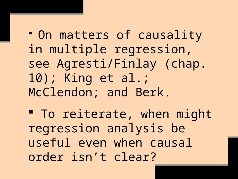
On matters of causality in multiple regression, see Agresti/Finlay (chap. 10); King et al.; McClendon; and Berk.
To reiterate, when might regression analysis be useful even when causal order isn’t clear?

Let’s turn our attention now to multiple regression, in which the outcome variable y is a function of k explanatory variables.
For every one-unit increase in x, y increases/decreases by … units on average, holding the other explanatory variables fixed.

Hence slope (i.e. regression) coefficients in multiple regression are commonly called ‘partial coefficients.’
They indicate the independent effect of a given explanatory variable x on y, holding the other explanatory variables constant.

Some other ways of saying ‘holding the other variables constant’:
holding the other variables fixed
adjusting for the other variables
net of the other variables

Statistical controls mimic experimental controls.
The experimental method, however, is unparalleled in its ability to isolate the effects of explanatory ‘treatment’ variables on an outcome variable, holding other variables constant.

What’s the effect of the daily amount of Cuban coffee persons drink on their levels of displayed anger, holding constant income, education, gender, race-ethnicity, body weight, health, mental health, diet, exercise, & so on?
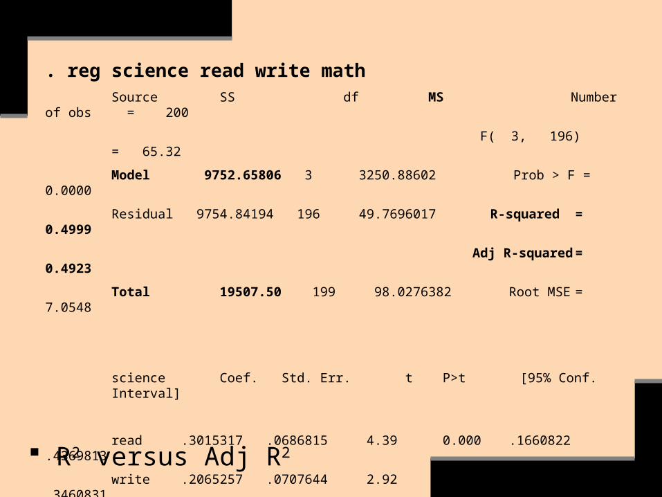
A Multiple Regression Example
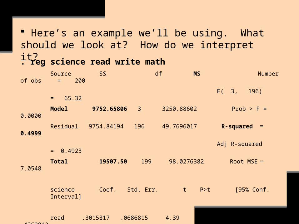
. reg science read write mathSource SS df MS Number of obs = 200
F( 3, 196) = 65.32
Model 9752.65806 3 3250.88602 Prob > F = 0.0000
Residual 9754.84194 196 49.7696017 R-squared = 0.4999
Adj R-squared = 0.4923
Total 19507.50 199 98.0276382 Root MSE = 7.0548
science Coef. Std. Err. t P>t [95% Conf. Interval]
read .3015317 .0686815 4.39 0.000 .1660822 .4369813
write .2065257 .0707644 2.92 0.004 .0669683 .3460831
math .3190094 .0766753 4.16 0.000 .167795 .4702239
_cons 8.407353 3.192799 2.63 0.009 2.110703 14.704
Here’s an example we’ll be using. What should we look at? How do we interpret it?

Here’s a standard deviation interpretation:
. su science read write math
. pcorr science read write math
Variable | Obs Mean Std. Dev. Min Max
-------------+--------------------------------------------------------
science | 200 51.85 9.900891 26 74
read | 200 52.23 10.25294 28 76
write | 200 52.775 9.478586 31 67
math | 200 52.645 9.368448 33 75
Partial correlation of science with
Variable | Corr. Sig.
-------------+------------------
read | 0.2992 0.000
write | 0.2041 0.004
math | 0.2849 0.000
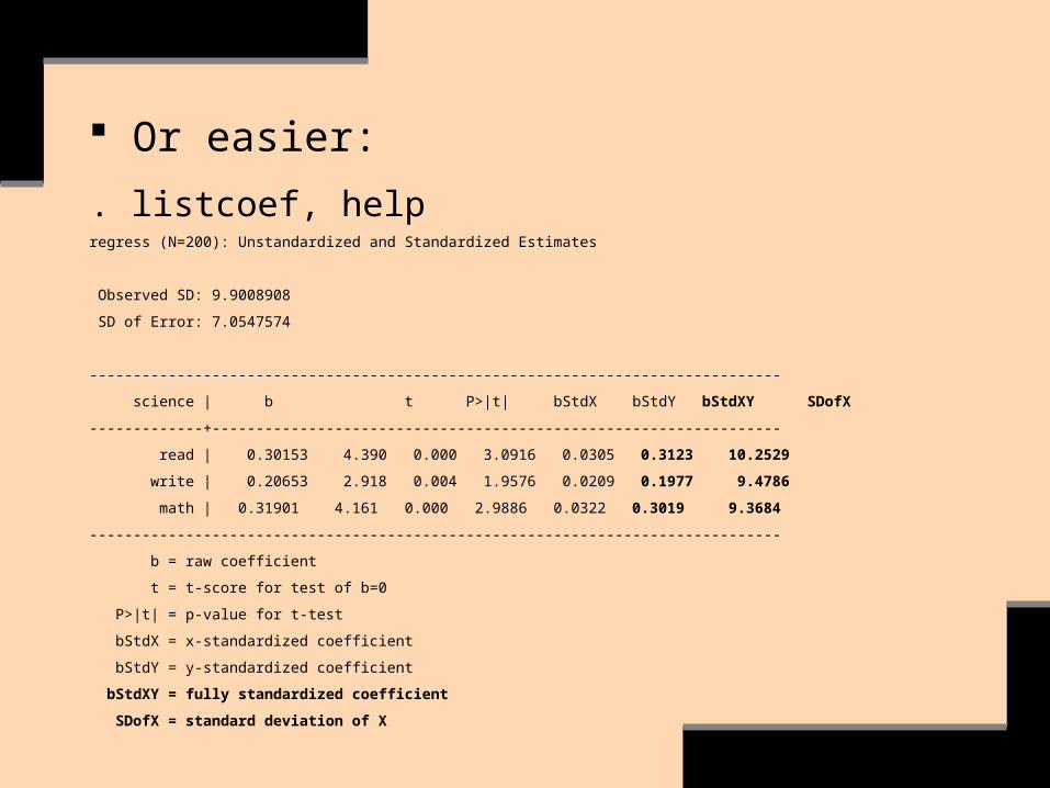
Or easier:
. listcoef, helpregress (N=200): Unstandardized and Standardized Estimates
Observed SD: 9.9008908
SD of Error: 7.0547574
-------------------------------------------------------------------------------
science | b t P>|t| bStdX bStdY bStdXY SDofX
-------------+-----------------------------------------------------------------
read | 0.30153 4.390 0.000 3.0916 0.0305 0.3123 10.2529
write | 0.20653 2.918 0.004 1.9576 0.0209 0.1977 9.4786
math | 0.31901 4.161 0.000 2.9886 0.0322 0.3019 9.3684
-------------------------------------------------------------------------------
b = raw coefficient
t = t-score for test of b=0
P>|t| = p-value for t-test
bStdX = x-standardized coefficient
bStdY = y-standardized coefficient
bStdXY = fully standardized coefficient
SDofX = standard deviation of X

Although multiple regression is linear in its parameters, we’ll see that it readily accommodates non-linearity in y/x relationships.
What would be possible non-linearity in the relationship between daily amounts of Cuban coffee people drink & their levels of displayed anger?
What about the preceding regression example?

. reg science read write math
Source SS df MS Number of obs = 200
F( 3, 196) = 65.32
Model 9752.65806 3 3250.88602 Prob > F = 0.0000
Residual 9754.84194 196 49.7696017 R-squared = 0.4999
Adj R-squared = 0.4923
Total 19507.50 199 98.0276382 Root MSE = 7.0548
science Coef. Std. Err. t P>t [95% Conf. Interval]
read .3015317 .0686815 4.39 0.000 .1660822 .4369813
write .2065257 .0707644 2.92 0.004 .0669683 .3460831
math .3190094 .0766753 4.16 0.000 .167795 .4702239
_cons 8.407353 3.192799 2.63 0.009 2.110703 14.704

We’ll later see that multiple regression coefficients are ‘partial coefficients.’
That is, the value (i.e. slope) of a given estimated regression coefficient may vary according to which other particular explanatory variables are included in the model.
Why?

. reg read write------------------------------------------------------------------------------
read | Coef. Std. Err. t P>|t| [95% Conf. Interval]
-------------+----------------------------------------------------------------
write | .64553 .0616832 10.47 0.000 .5238896 .7671704
. reg read write math------------------------------------------------------------------------------
read | Coef. Std. Err. t P>|t| [95% Conf. Interval]
-------------+----------------------------------------------------------------
write | .3283984 .0695792 4.72 0.000 .1911828 .4656141
math | .5196538 .0703972 7.38 0.000 .380825 .6584826
. reg read write math science------------------------------------------------------------------------------
read | Coef. Std. Err. t P>|t| [95% Conf. Interval]
-------------+----------------------------------------------------------------
write | .2376706 .0696947 3.41 0.001 .1002227 .3751184
math | .3784015 .0746339 5.07 0.000 .2312129 .5255901
science | .2969347 .0676344 4.39 0.000 .1635501 .4303192
Sources of Error in Regression Analysis
What are the three basic sources of error in regression analysis?

The three basic sources of error in regression analysis are:
(1) Sampling error
(2) Measurement error (including all types of non-sampling error)
(3) Omitted variables
Source: Allison (pages 14-16)
How do we evaluate error in a model?

We evaluate error in a model by means of:
(1) Evaluating the sample for sampling & non-sampling error
(2) Our substantive knowledge about the topic (e.g., what are the most important variables; how they should be defined & measured)
(3) Confidence intervals & hypothesis tests
(a) F-test of global utility
(b) Confidence intervals & hypothesis tests for regression coefficients
(4) Post-model diagnostics of residuals (i.e. ‘error’)

The evaluation of error involves assumptions about the random error component.
These assumptions are the same for multiple regression as for simple linear regression.
What are these assumptions? Why are they important?

How large must sample size n be for multiple regression?
It must be at least 10 observations per explanatory variable estimated (not including the constant, or y-intercept).
In reality the sample size n should be even larger—quite large, in fact. Why? (See R2 below.)

As with simple linear regression, multiple regression fits a least squares line that minimizes the sum of squared errors (i.e. the sum of squared deviations between predicted and observed y values).
The formulas for multiple regression, however, are more complex than those for simple regression.

Estimating the variance of e (i.e. of yhat) with k explanatory variables:
degrees of freedom =
n – (# explanatory vars estimated + constant)
1)](k-[n
SSE
Error forSquare Means
2
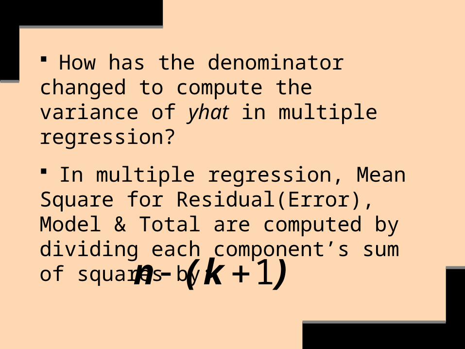
How has the denominator changed to compute the variance of yhat in multiple regression?
In multiple regression, Mean Square for Residual(Error), Model & Total are computed by dividing each component’s sum of squares by:
)k(n 1

Estimating the standard error of e (i.e. of yhat):
2ss

Testing an individual parameter coefficient in multiple regression:
kkx...xxy 22110
Ho: = 0
Ha: 0
11
11 sˆt
(or one-sided test in either direction)
1)](k-[ndf
Assumptions about sample; assumptions about e: I.I.D.

Multiple coefficient of determination, R2
2)yy(SSE ii
2)yy(SSyy i
y
SSyy
SSE-SSyyR2
: predicted values of y

R2: fraction of the sample variation of the y values (measured by SSyy) that is attributable to the regression model (i.e. to the explanatory variables).
Note: r2 versus R2

. reg science read write mathSource SS df MS Number of obs = 200
F( 3, 196) = 65.32
Model 9752.65806 3 3250.88602 Prob > F = 0.0000
Residual 9754.84194 196 49.7696017 R-squared = 0.4999
Adj R-squared = 0.4923
Total 19507.50 199 98.0276382 Root MSE = 7.0548
science Coef. Std. Err. t P>t [95% Conf. Interval]
read .3015317 .0686815 4.39 0.000 .1660822 .4369813
write .2065257 .0707644 2.92 0.004 .0669683 .3460831
math .3190094 .0766753 4.16 0.000 .167795 .4702239
_cons 8.407353 3.192799 2.63 0.009 2.110703 14.704
R2=SSModel/SSTotal=9752.65806/19507.50

Caution: R2 for a regression model may vary considerably from sample to sample (due to chance associations); i.e. it does not necessarily reveal the model’s fit for the population.
Caution: R2 will be overestimated if a sample doesn’t contain substantially more data points than the number of explanatory variables (rule of thumb: at least 30 observations per explanatory variable; an overall sample size of at least 400).

Caution: in view of the preceding, R2 gets larger with the addition of more explanatory variables.
Adjusted R2 adjusts both for the sample size n & for the number of explanatory variables; thus it gives a more stable & conservative estimate.
R2 & Adj R2, however, are sample statistics that do not have associated hypothesis tests.
. reg science read write mathSource SS df MS Number of obs = 200
F( 3, 196) = 65.32
Model 9752.65806 3 3250.88602 Prob > F = 0.0000
Residual 9754.84194 196 49.7696017 R-squared = 0.4999
Adj R-squared = 0.4923
Total 19507.50 199 98.0276382 Root MSE = 7.0548
science Coef. Std. Err. t P>t [95% Conf. Interval]
read .3015317 .0686815 4.39 0.000 .1660822 .4369813
write .2065257 .0707644 2.92 0.004 .0669683 .3460831
math .3190094 .0766753 4.16 0.000 .167795 .4702239
_cons 8.407353 3.192799 2.63 0.009 2.110703 14.704
R2 versus Adj R2

Neither R2 nor Adj R2, then, should be the sole or primary measure for judging a model’s usefulness.
The first, & most basic, test for judging a model’s usefulness is the Analysis of Variance F Test.

Analysis of Variance F-Test for the overall utility of a multiple regression model:
Ho: 021 k... Ha: at least one differs from 0.i
error forsquare meanmodel forsquare meanF
1)](k-[nSSEkSS(Model)/
F F:region Rejection

An alternative formula uses R2:
error forsquare meanmodel forsquare meanF
1)](k-[nR2)-(1
R2/k

. reg science read write mathSource SS df MS Number of obs = 200
F( 3, 196) = 65.32
Model 9752.65806 3 3250.88602 Prob > F = 0.0000
Residual 9754.84194 196 49.7696017 R-squared = 0.4999
Adj R-squared = 0.4923
Total 19507.50 199 98.0276382 Root MSE = 7.0548
science Coef. Std. Err. t P>t [95% Conf. Interval]
read .3015317 .0686815 4.39 0.000 .1660822 .4369813
write .2065257 .0707644 2.92 0.004 .0669683 .3460831
math .3190094 .0766753 4.16 0.000 .167795 .4702239
_cons 8.407353 3.192799 2.63 0.009 2.110703 14.704
F=MSModel/MSResidual

We either reject or fail to reject Ho for the F-test.
If we fail to reject Ho, then we don’t bother assessing the other indicators of model usefulness & fit: instead we go back to the drawing board, revise the model, & try again.

Regarding the F-test, note that the formula expresses the parsimony of explanation that’s fundamental to the culture of ‘scientific explanation’ (see King et al., page 20).
That is, too many explanatory variables relative to the number of observations decreases the degrees of freedom & thus makes statistical significance more difficult to obtain.

Why not assess the model’s overall utility by doing hypothesis tests based on t-values?
Probability of Type I error.
Why not use R2 or Adj R2?
Because there’s no hypothesis test for R2 or Adj R2.

If, on the other hand, the F-test does reject Ho, then do go on to conduct the t-value hypothesis tests.
But watch out for Type I errors.

In any case, rejecting Ho based on the F-test does not necessarily imply that this is the best model for predicting y.
Another model might also pass the F-test & prove even more useful in providing estimates & predictions.

Before going on with multiple regression, let’s review some basic issues of causality (see Agresti & Finlay, chapter 10; King et al., chapter 3).
In causal relations, one variable influences the other, but not vice versa.
We never definitively prove causality, but we can (more or less) disprove causality (over the long run of accumulated evidence).

A relationship must satisfy three criteria to be (tentatively) considered causal:
(1) An association between the variables
(2) An appropriate time order
(3) The elimination of alternative explanations

Association & time order do not necessarily amount to causality.
Alternative explanations must be eliminated.

But first, does a finding of statistical insignificance necessarily mean that there’s no causal relationship between y & x?
It could be that:
(1) The y/x relationship is nonlinear: perhaps linearize it via transformation.
(2) The y/x relationship is contingent on controlling another explanatory variable that has been omitted, or else on the level of another variable (i.e. interaction).
(3) The sample size is inadequate.
(4) There’s sampling error.
(5) There’s non-sampling error (including measurement error).

When there is statistical significance, an apparently causal relationship may in fact be:
Dependent on one or more lurking variables (i.e. spurious relationship: x2 causes x1 & x2 causes y, so there is no x1 causal relationship with y).
Mediated by an intervening variable (i.e. chain: x1
indirectly causes y via x2).
Conditional on the level of another variable (i.e. interaction).
An artifact of an extreme value on the sampling distribution of the sample mean.

On such complications of causality, see Agresti/Finlay, chapter 10; McClendon; Berk; and King et al.

How to detect at least some of the possible lurking variables:
Add suspected lurking variables (x2-xk) to the model.
Does the originally hypothesized y/ x1 relationship remain significant or not?

E.g., for pre-adolescents, there’s a strong relationship between height & math achievement scores.
Does the relationship between height & math scores remain when we control for age? If not, the height/math relationship is spurious, because both math depends on age & height depends on age.
What other explanatory variables might be relevant?

The case of spurious associations (i.e. lurking variables) is one example of a multivariate relationship.
Another kind is a chain relationship. E.g.:
rate arrestincomefamily race
Race affects arrest rate, but controlling for specific levels of family income makes the unequal white/nonwhite arrest rate diminish. Race’s effect is mediated by family income.
yx2x1

The difference between a chain (i.e. mediated) relationship & a spurious relationship is in the conceptual order:
rate arrestincomefamily race
rate arrestraceincomefamily
yx2x1
yx1x2 In this example, the former is chain, the latter is spurious: Why?

How can we conceptualize Weber’s ‘Protestant ethic/spirit of capitalism’ argument within the framework of chain vs. spurious causality? (see King et al., pages 186-87).

E.g.: mediation & spurious relation
. use crime, clear
. reg crime pctmetro------------------------------------------------------------------------------
crime | Coef. Std. Err. t P>|t| [95% Conf. Interval]
-------------+----------------------------------------------------------------
pctmetro | 10.92928 2.408001 4.54 0.000 6.090222 15.76834
_cons | -123.6833 170.5113 -0.73 0.472 -466.3387 218.972
------------------------------------------------------------------------------
. reg crime pctmetro pctwhite------------------------------------------------------------------------------
crime | Coef. Std. Err. t P>|t| [95% Conf. Interval]
-------------+----------------------------------------------------------------
pctmetro | 7.155473 2.017343 3.55 0.001 3.099334 11.21161
pctwhite | -18.5332 3.340908 -5.55 0.000 -25.25054 -11.81585
_cons | 1689.567 353.4511 4.78 0.000 978.9061 2400.228

. reg crime pctmetro pctwhite poverty------------------------------------------------------------------------------
crime | Coef. Std. Err. t P>|t| [95% Conf. Interval]
-------------+----------------------------------------------------------------
pctmetro | 8.848472 1.767408 5.01 0.000 5.292905 12.40404
pctwhite | -12.54453 3.171839 -3.95 0.000 -18.92545 -6.163611
poverty | 37.46717 8.652025 4.33 0.000 20.06154 54.8728
_cons | 537.4967 402.4612 1.34 0.188 -272.1508 1347.144
. reg crime pctmetro pctwhite poverty single-----------------------------------------------------------------------------
crime | Coef. Std. Err. t P>|t| [95% Conf. Interval]
-------------+----------------------------------------------------------------
pctmetro | 7.404075 1.284941 5.76 0.000 4.817623 9.990527
pctwhite | -3.509082 2.639226 -1.33 0.190 -8.821568 1.803404
poverty | 16.66548 6.927095 2.41 0.020 2.721964 30.609
single | 120.3576 17.8502 6.74 0.000 84.42702 156.2882
_cons | -1191.689 386.0089 -3.09 0.003 -1968.685 -414.6936

Redundancy is when an independent variable’s coefficient diminishes when another independent variable is added to the model.
The pattern of correlations determines whether & to what degree this happens.

. corr crime murder pctmetro pctwhite poverty single | crime murder pctmetro pctwhite poverty single
-------------+------------------------------------------------------
crime | 1.0000
murder | 0.8862 1.0000
pctmetro | 0.5440 0.3161 1.0000
pctwhite | -0.6772 -0.7062 -0.3372 1.0000
poverty | 0.5095 0.5659 -0.0605 -0.3893 1.0000
single | 0.8389 0.8589 0.2598 -0.6564 0.5486 1.0000
Redundancy occurs when, for the particular two variables in question, each one’s correlation with y is greater than the other independent variable’s correlation with y times the correlation between the two independent variables.

. r crime-pctwhite=-.6772
. r crime-single*r pctwhite-single=.8389*
-.6564=-.55065396
-.5507 is greater than -.6772, thus reducing pctwhite’s coefficient in the regression model.
That is, the variances of these regression coefficients overlap, with ‘single’ containing much of the variance of ‘pctwhite’.
This occurs to the extent that holding ‘single’ constant turns ‘pctwhite’ insignificant.
What might this mean substantively?

Some other kinds of multivariate relationships:
Suppressor variable: a bivariate relationship appears only when a third variable is controlled.
Simpson’s Paradox (a version of ‘suppression’): the direction of a bivariate relationship changes when a third variable is added.
Statistical interaction: the strength of a bivariate association changes according to the value of a third variable (e.g., if the income return on years of education is greater for males than females, or greater for whites than nonwhites).
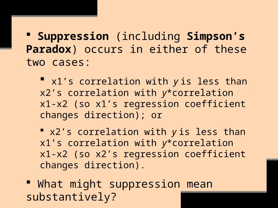
Suppression (including Simpson’s Paradox) occurs in either of these two cases:
x1’s correlation with y is less than x2’s correlation with y*correlation x1-x2 (so x1’s regression coefficient changes direction); or
x2’s correlation with y is less than x1’s correlation with y*correlation x1-x2 (so x2’s regression coefficient changes direction).
What might suppression mean substantively?
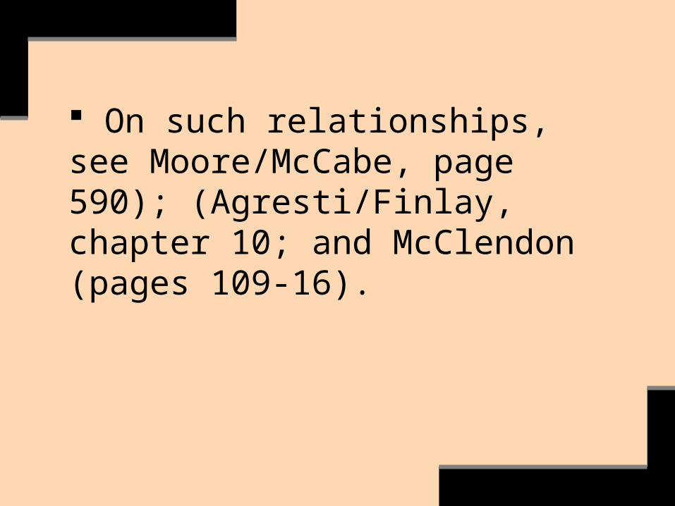
On such relationships, see Moore/McCabe, page 590); (Agresti/Finlay, chapter 10; and McClendon (pages 109-16).

Remember, however, that any finding of statistical significance (or insignificance) may be an artifact of an extreme value on the sampling distribution of the sample mean (i.e. sampling error) or of non-sampling error.
Conclusions are always uncertain (see King et al., pages 31-32).

Introduction to Types of Linear Models
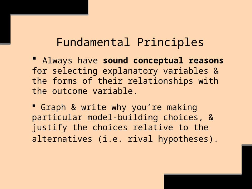
Fundamental Principles Always have sound conceptual reasons for selecting explanatory variables & the forms of their relationships with the outcome variable.
Graph & write why you’re making particular model-building choices, & justify the choices relative to the alternatives (i.e. rival hypotheses).

Always be skeptical.
Ask ‘What kind of evidence would force me to revise or reject my model?’ (see King et al. & Ragin).
And always connect such evidence to theories, models, & hypotheses.

A theory is “a reasoned and precise speculation about the answer to a research question, including a statement about why the proposed answer is correct.”
“Theories usually imply several more specific descriptive or causal hypotheses” (King et al., page 19).
A model is “a simplification of, and approximation to, some aspect of the world. Models are never literally ‘true’ or ‘false,’ although good models abstract only the ‘right’ features of the reality they represent” (King et al., page 49).

Models with quantitative x’s
kkx...xy 110
. u hsb2, clear
. reg science read write math socst
A first-order linear model
How well does the model fit the data?

. reg science read write math socst
Source SS df MS Number of obs = 200
F( 4, 195) = 48.80
Model 9758.84934 4 2439.71233 Prob > F = 0.0000
Residual 9748.65066 195 49.9930803 R-squared = 0.5003
Adj R-squared = 0.4900
Total 19507.50 199 98.0276382 Root MSE = 7.0706
science Coef. Std. Err. t P>t [95% Conf. Interval]
read .3099891 .0729101 4.25 0.000 .1661955 .4537826
write .2149167 .074824 2.87 0.005 .0673486 .3624849
math .3218104 .0772583 4.17 0.000 .1694412 .4741795
socst -.0227148 .0645465 -0.35 0.725 -.1500137 .1045842
_cons 8.5657 3.23144 2.65 0.009 2.192642 14.93876
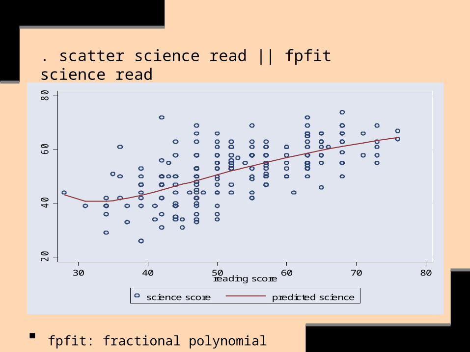
. scatter science read || fpfit science read2
04
06
08
0
30 40 50 60 70 80reading score
science score predicted science
fpfit: fractional polynomial

. scatter science write || fpfit science write2
04
06
08
0
30 40 50 60 70writing score
science score predicted science

. scatter science math || fpfit science math2
04
06
08
0
30 40 50 60 70 80math score
science score predicted science
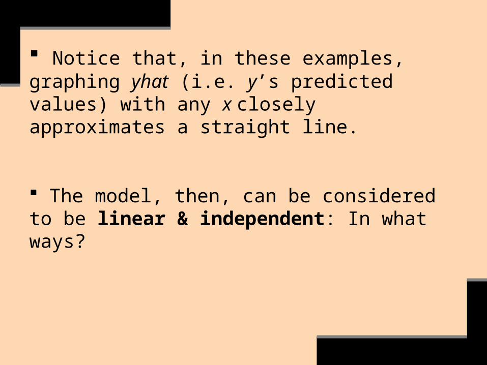
Notice that, in these examples, graphing yhat (i.e. y’s predicted values) with any x closely approximates a straight line.
The model, then, can be considered to be linear & independent: In what ways?

Linear, independent: if we hold all the other explanatory variables constant & vary only x1, the expected value of y will change by the amount of the corresponding regression coefficient for every unit change in x1.
We look for reasonable approximations of this model.

If the y/x relationships are substantially non-linear, then the non-linearity is likely to emerge in STATA’s ‘qfit’ or ‘fpfit’ scatter plots.
We did not find much evidence of this, however.
Let’s further explore this matter via STATA’s ‘sparl’ (downloadable ‘scatter plot & regression line’) graphs.

science = 16.412 + 0.751 read - 0.001 read 2r² = 0.397 RMSE = 7.725 n = 200
scie
nce s
core
reading score20 40 60 80
20
40
60
80
sparl science read, quad
sparl is a quick & helpful exploratory tool.

exxxxy 21322110
An interaction model with quantitative variables
. u WAGE1, clear

An interaction model incorporates the possibility of curvilinearity.
In the case of this model, then, education & job tenure do not exert independent, linear effects on predicted earnings.
Instead, the relationship of job tenure to y is hypothesized as varying according to the level of education, & vice versa.

If interacting variables test significant, then the slopes are unequal.
E.g., different earnings/ education slope for women versus men.

This is one of many examples we’ll cover concerning the use of a linear model to fit curvilinear relationships (including, e.g., using log of wage, the outcome variable).

Notice the structure of the model: it must include each stand-alone explanatory variable, which serve together as the foundation on which the interaction term is based.
exxxxy 21322110

Let’s begin by exploring if regressing wage on tenure & wage on education take some curvilinear forms.
We can explore these possibilities of curvilinearity, before estimating a regression equation, via the following graph:

. scatter wage tenure || qfit wage tenure0
510
15
20
25
avera
ge h
ourl
y e
arn
ings/F
itte
d v
alu
es
0 10 20 30 40years w ith current employer
average hourly earnings Fitted values

sparl wage tenure, quad
wage = 4.659 + 0.341 tenure - 0.006 tenure 2r² = 0.138 RMSE = 3.434 n = 526
avera
ge h
ourly e
arn
ings
years with current employer0 20 40
0
10
20
30

. scatter wage educ || qfit wage educ0
510
15
20
25
avera
ge h
ourl
y e
arn
ings/F
itte
d v
alu
es
0 5 10 15 20years of education
average hourly earnings Fitted values

sparl wage educ, quad
wage = 5.408 - 0.607 educ + 0.049 educ 2r² = 0.201 RMSE = 3.307 n = 526
avera
ge h
ourly e
arn
ings
years of education0 5 10 15 20
0
10
20
30

We’ll hypothesize that the curvilinearity takes the form of interaction between tenure & education:
exxxxy 21322110
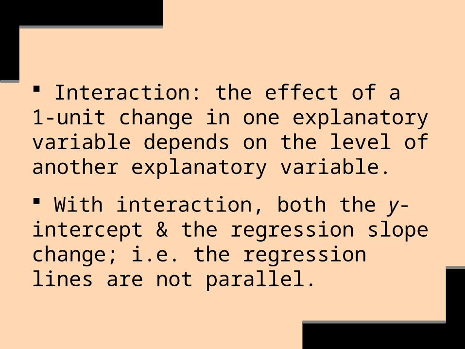
Interaction: the effect of a 1-unit change in one explanatory variable depends on the level of another explanatory variable.
With interaction, both the y-intercept & the regression slope change; i.e. the regression lines are not parallel.

. gen tenureXeduc=tenure*educ
. for varlist tenure educ tenureXeduc: hist X / more
. su tenure educ tenureXeduc, d
Let’s create the interaction variable:

. reg wage educ tenure educXtenure
. Note: I used wage, rather than lwage, for the heuristic purposes of this example because the former, but not the latter, tests significant. In our real research we’d use lwage. Why?

. reg wage educ tenure educXtenure
Source | SS df MS Number of obs = 526
-------------+------------------------------ F( 3, 522) = 82.15
Model | 2296.41715 3 765.472384 Prob > F = 0.0000
Residual | 4863.99714 522 9.31800218 R-squared = 0.3207
-------------+------------------------------ Adj R-squared = 0.3168
Total | 7160.41429 525 13.6388844 Root MSE = 3.0525
------------------------------------------------------------------------------
wage | Coef. Std. Err. t P>|t| [95% Conf. Interval]
-------------+----------------------------------------------------------------
educ | .4265947 .0610327 6.99 0.000 .3066948 .5464946
tenure | -.0822392 .0737709 -1.11 0.265 -.2271635 .0626851
educXtenure | .0225057 .0059134 3.81 0.000 .0108887 .0341228
_cons | -.4612881 .7832198 -0.59 0.556 -1.999938 1.077362
------------------------------------------------------------------------------

If the interaction term tests significant, we don’t concern ourselves with the statistical significance or regression coefficients of its stand-alone components (e.g., x1, x2).
The statistically significant interaction term with a positive coefficient indicates some degree of positive curvilinearity in the relationship of yhat to x1*x2.

We can graph the interaction effect of two continuous variables if we estimate the regression model using Stata’s downloadable ‘xi3’ command (see UCLA-ATS: ‘STATA FAQ: How do I use xi3?’)
. xi3:reg wage educ*tenure
Note: we list the explanatory variables differently when using xi3.

. scatter wage _IedXte || qfit wage _IedXte
0
5
10
15
20
25
0 200 400 600educ*tenure
average hourly earnings Fitted values

This interaction graph doesn’t allow us to see the amount of change per unit of education or tenure.
So here’s what we typically do:

Using y/x scatterplots, ‘su x1, d’ & our knowledge of the subject, we identify key levels of tenure & educ (or alternatively, one SD or quartile above mean/median, mean/median, & one SD below mean/median).
Then we predict the slope-effect of tenureXeduc on wage at these key levels, as follows:

How the interaction of mean tenure with varying levels of education predicts wage:
. lincom tenure + (tenureXeduc*8)
wage Coef. Std. Err. t P>t [95% Conf. Interval]
(1) .0978065 .0303746 3.22 0.001 .0381351 .157478
. lincom tenure + (tenureXeduc*12)
wage Coef. Std. Err. t P>t [95% Conf. Interval]
(1) .1878294 .0184755 10.17 0.000 .1515338 .224125
. lincom tenure + (tenureXeduc*20)
wage Coef. Std. Err. t P>t [95% Conf. Interval]
(1) .3678751 .0503567 7.31 0.000 .2689484 .4668019
The slope-coefficients & y-intercept change.

0
5
10
15
20
25
0 200 400 600educ*tenure
average hourly earnings Fitted values

How the interaction of mean education with varying levels of tenure predicts wage:. lincom educ + (2*tenureXeduc)
wage Coef. Std. Err. t P>t [95% Conf. Interval]
(1) -.0372278 .062391 -0.60 0.551 -.1597961 .0853406
. lincom educ + (10*tenureXeduc)
wage Coef. Std. Err. t P>t [95% Conf. Interval ]
(1) .142818 .0221835 6.44 0.000 .0992382 .1863978
. lincom educ + (18*tenureXeduc)
wage Coef. Std. Err. t P>t [95% Conf. Interval]
(1) .3678751 .0503567 7.31 0.000 .2689484 .4668019
The slope-coefficients & y-intercept change.

For a clearly explained example, see Allison, pages 166-69.
How does the principle of interaction differ from that of linear, independent effects?

Interacting variables may be quantitative, categorical, or a combination of the two:
. yrstenureXyrseduc: quantitative
. ethnic_groupXgender: categorical
. genderXyrseduc: combination categorical & quantitative

Two Sources of Interaction Effects
Sociologist Richard Williams (U. Notre Dame) emphasizes that there are two sources of interaction effects (see his web notes):
(1) Compositional differences between groups: the means of groups on an explanatory variable (e.g., mean of education, income) may differ.

(2) The effects of an explanatory variable may differ between groups.
Why, conceptually, is it important to recognize these two sources of interaction effects?
Williams recommends using, e.g., a ttest to assess #1 before estimating a model: ttest educ, by(gender).

Regarding #1 & #2, Williams suggests the following:
Estimate a separate model for each group (e.g., for women & for men).
Estimate an interaction model for gender.
Test the latter model for nested model significance.
Given earlier ttest, keep in mind the two sources of interaction effects.

Williams also suggests the following strategy:
Estimate a model for one group only (e.g., women).
Then use the ‘predict’ command to predict yhat for the other group only:
. predict yhat if ~=women
. su yhat

This yields the predicted values for a hypothetical group that has men’s mean values for the explanatory variables, but it displays the slopes (i.e. effects) for women.

Interpretation: What would be the predicted values for women if they had men’s mean values on the explanatory variables—lower predicted values, the same, or higher?
You could use, e.g., lincom to explore this question.
Note: Recall last semester’s discussion of Simpson’s Paradox—How is this discussion relevant to that?
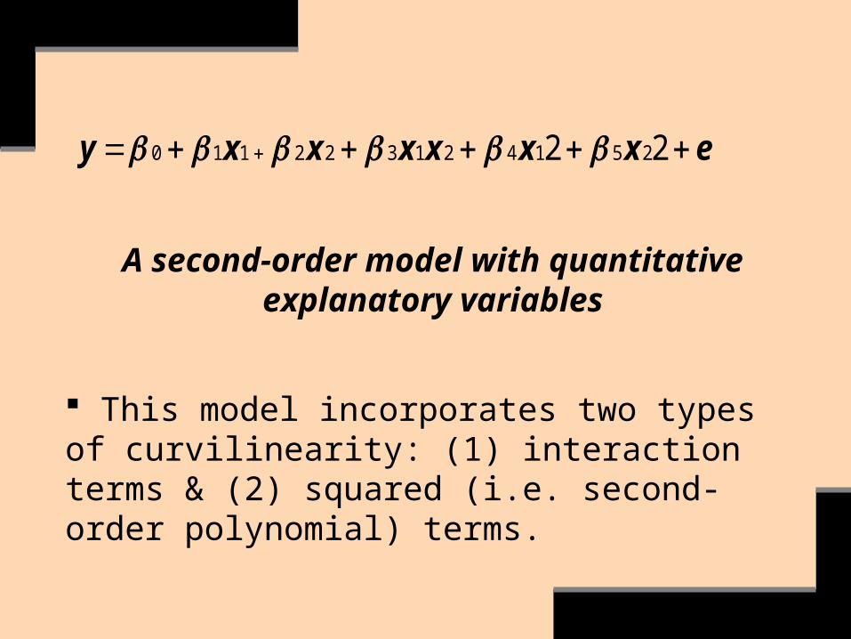
A second-order model with quantitative explanatory variables
This model incorporates two types of curvilinearity: (1) interaction terms & (2) squared (i.e. second-order polynomial) terms.
exxxxxxy 22 251421322110
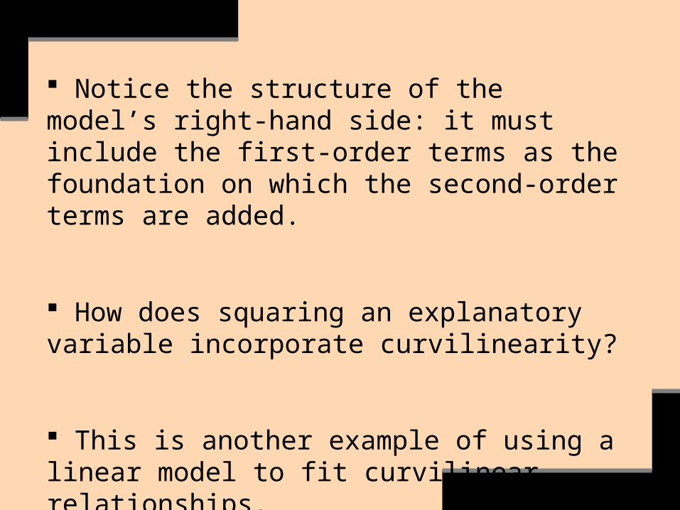
Notice the structure of the model’s right-hand side: it must include the first-order terms as the foundation on which the second-order terms are added.
How does squaring an explanatory variable incorporate curvilinearity?
This is another example of using a linear model to fit curvilinear relationships.

Observe the form of the model containing the squared term: it must include the corresponding first-order term, which forms the foundation on which the squared term is based.
exxxxxxy 22 251421322110
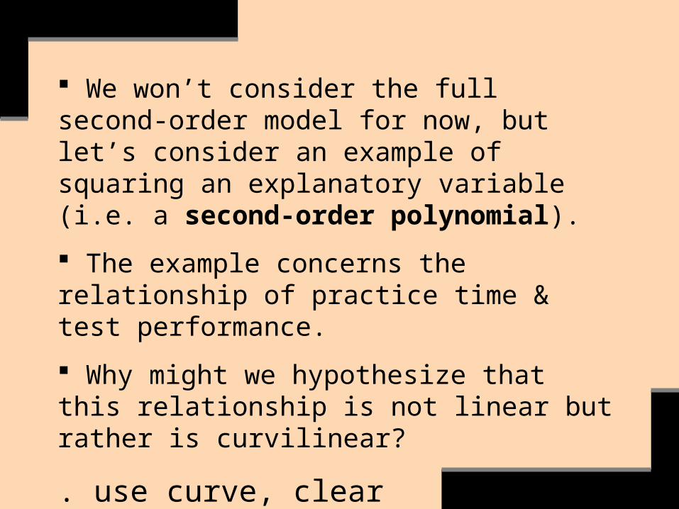
We won’t consider the full second-order model for now, but let’s consider an example of squaring an explanatory variable (i.e. a second-order polynomial).
The example concerns the relationship of practice time & test performance.
Why might we hypothesize that this relationship is not linear but rather is curvilinear?
. use curve, clear

. scatter numcor prtime || qfit numcor prtime5
10
15
20
y/F
itte
d v
alu
es
2 4 6 8 10 12x
y Fitted values

num_correct = -2.236 + 4.152 prac_time - 0.210 prac_time 2r² = 0.810 RMSE = 2.680 n = 18
=y
=x0 5 10 15
5
10
15
20
. sparl num_cor prac_time, quad

Let’s try to fit this curvilinear relationship.
A basic way of doing so is to square the explanatory variable:
. gen prtimesq=prtime^2
. for var prtime prtimesq: hist X \ more
. su prctime prtimesq, d
. reg numcor prtime prtimesq

As with models containing interaction terms, if the squared explanatory variable tests significant we’re no longer concerned with the statistical significance or regression coefficient of the first-order variable (e.g., prtime).

By comparing the distribution of their residuals, let’s graphically compare the fit of the following two models:
. reg numcor prtime
. reg numcor prtime prtimesq

. reg numcor prtime
. rvfplot, yline(0)
What’s the problem here?
-10
-50
5
Fitte
d v
alu
es
5 10 15 20Residuals

. reg numcor prtime prtimesq
. rvfplot, yline(0)
There’s improvement.
-10
-50
5
Fitte
d v
alu
es
5 10 15 20Residuals

. reg numcor prtime prtimesq
Source | SS df MS Number of obs = 18
-------------+------------------------------ F( 2, 15) = 31.90
Model | 458.245766 2 229.122883 Prob > F = 0.0000
Residual | 107.754234 15 7.18361562 R-squared = 0.8096
-------------+------------------------------ Adj R-squared = 0.7842
Total | 566.00 17 33.2941176 Root MSE = 2.6802
------------------------------------------------------------------------------
numcor | Coef. Std. Err. t P>|t| [95% Conf. Interval]
-------------+----------------------------------------------------------------
prtime | 4.151667 .8872181 4.68 0.000 2.260607 6.042728
prtimesq | -.209529 .0635329 -3.30 0.005 -.3449462 -.0741119
_cons | -2.236083 2.55445 -0.88 0.395 -7.680764 3.208598
Interpretation?

Let’s graph yhat. For a second-order (i.e. quadratic) model, Stata gives us two ways to produce the graph. Here’s the hard way:
. predict yhat if e(sample)
. predict se, stdp
. di(invttail 17, .05/2)
2.11
. gen lo = yhat – (2.11*se)
. gen hi = yhat + (2.11*se)

. scatter numcor yhat lo hi prtime, sort c(. l l l) m(o i i i)
05
10
15
20
y/F
itte
d v
alu
es/lo/h
i
2 4 6 8 10 12x
y Fitted values
lo hi

00
55
1010
1515
2020
y/F
itte
d va
lu
es/lo
/h
iy/F
itte
d va
lu
es/lo
/h
i
22 44 66 88 1010 1212xx
yy Fitted valuesFitted values lolohihi
. scatter numcor yhat lo hi prtime, sort
c(. l l l) m(o i i i) scheme(economist)

Here’s the easy way:
. twoway qfitci numcor prtime, bc(red)
05
10
15
20
95%
CI/F
itte
d v
alu
es
2 4 6 8 10 12x
95% CI Fitted values

Let’s next interpret the squared coefficient by predicting numcor at specific levels of prac_time (not prac_timesq).
We identify the specific levels via scatterplot, via su prac_time, d, & via our knowledge of the subject.
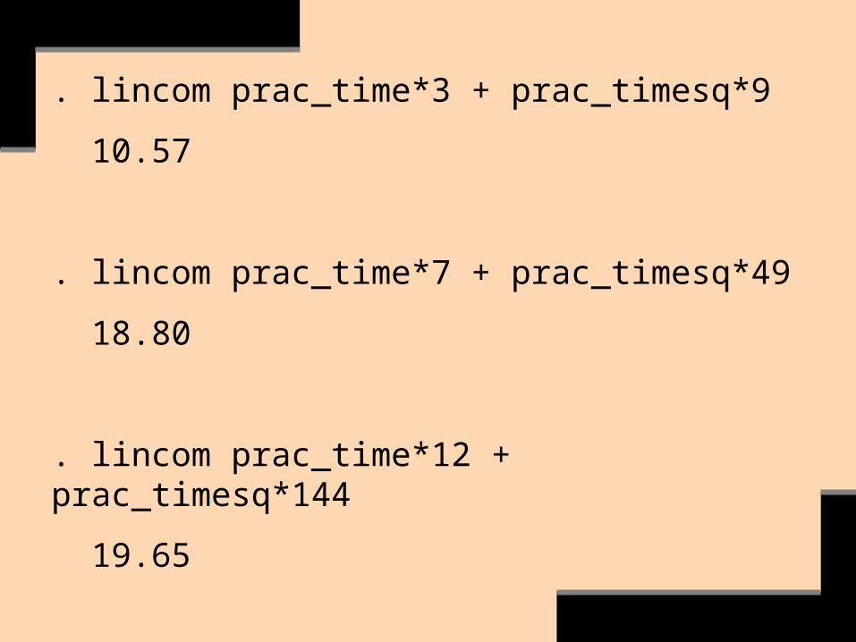
. lincom prac_time*3 + prac_timesq*9
10.57
. lincom prac_time*7 + prac_timesq*49
18.80
. lincom prac_time*12 + prac_timesq*144
19.65

Check to see if there’s a sufficient number of observations at each level to justify the interpretation at that level.
Otherwise the level’s finding may be an artifact of few or no observations.

We square only quantitative variables (interval or ratio). As with most transformations, a relatively wide range of values works best.
Rarely in the social sciences do we go higher than squaring quantitative variables (e.g., rarely do we cube variables).
Always ask: to what extent do gains in data fit come at the cost of interpretability?

A Model with a Two-level Categorical Explanatory Variable
. u hsb2, clear
Let’s consider a regression model to estimate a difference in the association of predicted science scores with whites versus nonwhites.
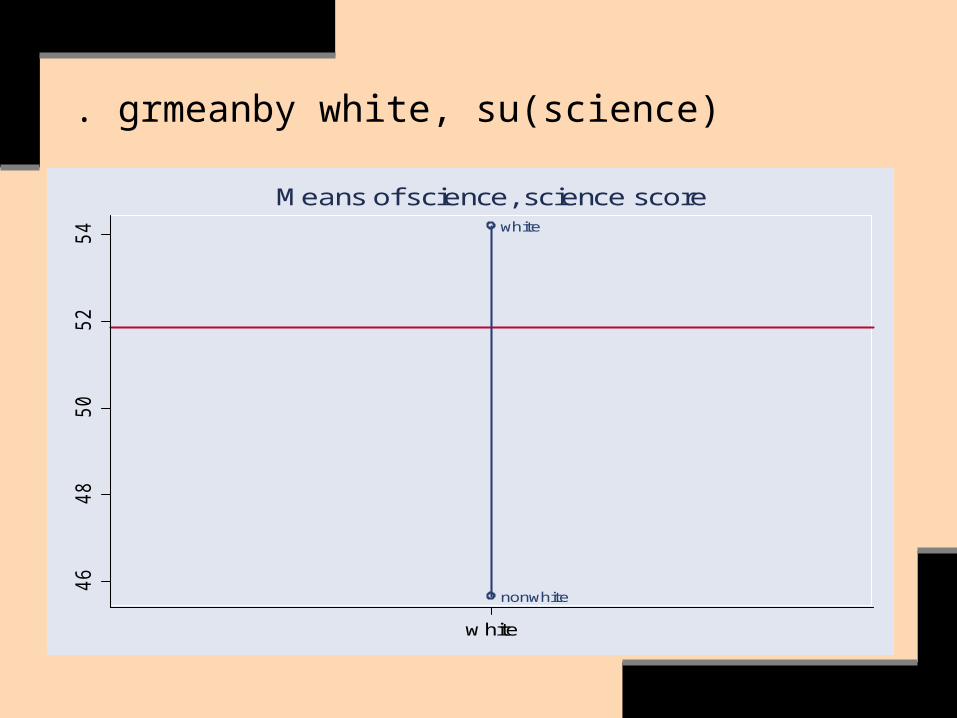
. grmeanby white, su(science)
white
nonwhite
46
48
50
52
54
w hite
Means of science, science score

Here’s the same evidence:
. bys white: su science
-> white = nonwhite
Variable | Obs Mean Std. Dev. Min Max
-------------+--------------------------------------------------------
science | 55 45.65455 9.313905 26 66
-> white = white
Variable | Obs Mean Std. Dev. Min Max
-------------+--------------------------------------------------------
science | 145 54.2 9.09487 33 74
or: tab white, su(science)

Is the relationship statistically significant?
. ttest science, by(white)Two-sample t test with equal variances
------------------------------------------------------------------------------
Group | Obs Mean Std. Err. Std. Dev. [95% Conf. Interval]
---------+--------------------------------------------------------------------
nonwhite | 55 45.65455 1.255887 9.313905 43.13664 48.17245
white | 145 54.2 .7552879 9.09487 52.70712 55.69288
---------+--------------------------------------------------------------------
combined | 200 51.85 .7000987 9.900891 50.46944 53.23056
---------+--------------------------------------------------------------------
diff | -8.545455 1.44982 -11.40452 -5.686385
------------------------------------------------------------------------------
Degrees of freedom: 198
Ho: mean(nonwhite) - mean(white) = diff = 0
Ha: diff < 0 Ha: diff != 0 Ha: diff > 0
t = -5.8941 t = -5.8941 t = -5.8941
P < t = 0.0000 P > |t| = 0.0000 P > t = 1.0000

. reg science white
Source SS df MS Number of obs = 200
F( 1, 198) = 34.74
Model 2911.8636 1 2911.86364 Prob > F = 0.0000
Residual 16595.6364 198 83.8163453 R-squared = 0.1493
Total 19507.5 199 98.0276382 Adj R-squared = 0.1450
Root MSE = 9.1551
science Coef. Std. Err. t P>t [95% Conf. Interval]
white 8.545455 1.44982 5.89 0.000 5.686385 11.40452
_cons 45.65455 1.234477 36.98 0.000 43.22014 48.08896

How well does the model fit?
What’s the interpretation?
The number of dummy variables used is one less than a categorical variable’s number of levels.
The comparison (or reference, or base) category is located within the equation’s constant-term (i.e. y-intercept).

Check the previous table:
The value of y-intercept?
The value of adding the coefficient ‘white’ to that of y-intercept?
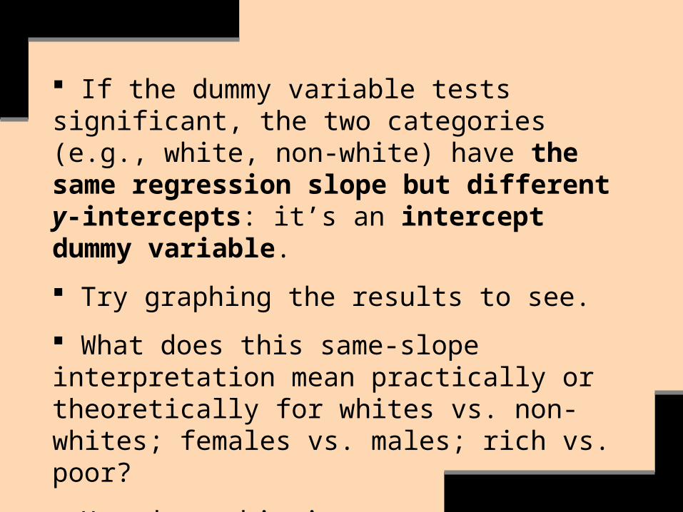
If the dummy variable tests significant, the two categories (e.g., white, non-white) have the same regression slope but different y-intercepts: it’s an intercept dummy variable.
Try graphing the results to see.
What does this same-slope interpretation mean practically or theoretically for whites vs. non-whites; females vs. males; rich vs. poor?
How does this interpretation compare to that of interaction slopes?

. reg science white
Source SS df MS Number of obs = 200
F( 1, 198) = 34.74
Model 2911.8636 1 2911.86364 Prob > F = 0.0000
Residual 16595.6364 198 83.8163453 R-squared = 0.1493
Total 19507.5 199 98.0276382 Adj R-squared = 0.1450
Root MSE = 9.1551
science Coef. Std. Err. t P>t [95% Conf. Interval]
white 8.545455 1.44982 5.89 0.000 5.686385 11.40452
_cons 45.65455 1.234477 36.98 0.000 43.22014 48.08896
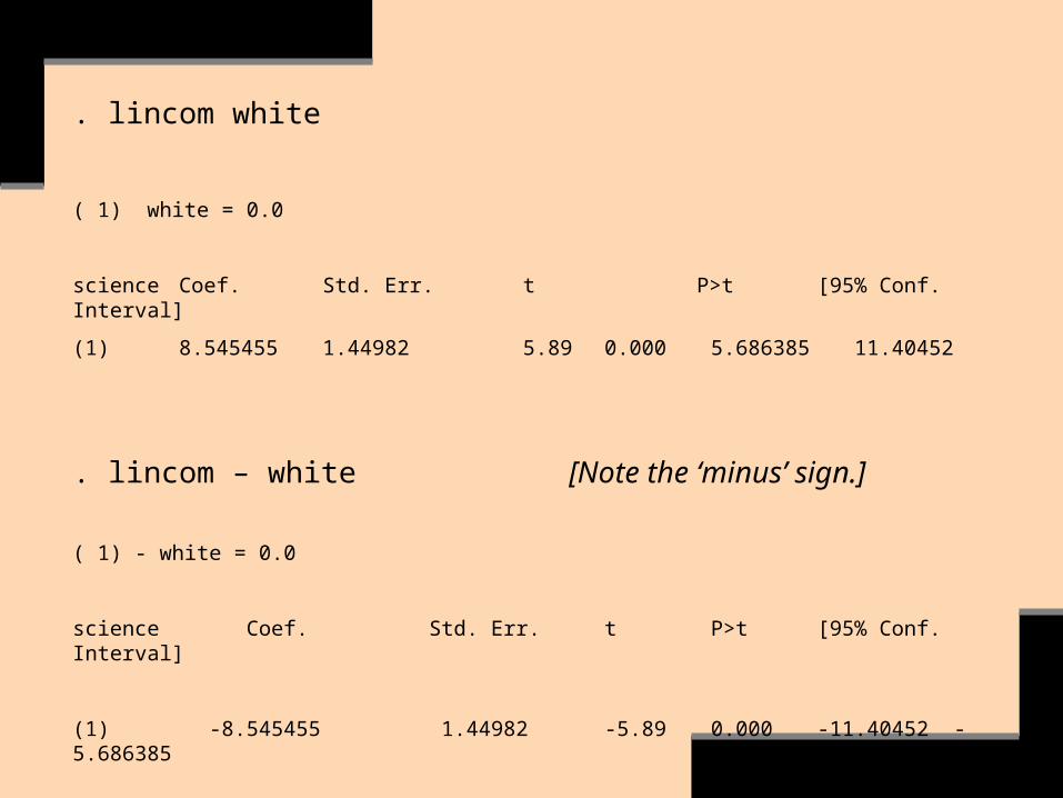
. lincom white
( 1) white = 0.0
science Coef. Std. Err. t P>t [95% Conf. Interval]
(1) 8.545455 1.44982 5.89 0.000 5.686385 11.40452
. lincom – white [Note the ‘minus’ sign.]
( 1) - white = 0.0
science Coef. Std. Err. t P>t [95% Conf. Interval]
(1) -8.545455 1.44982 -5.89 0.000 -11.40452 -5.686385

A Model with a Multi-level Nominal Categorical Explanatory Variable
. use hsb2, clear

. tab race
hispanic,
black,
asian,
white
Freq. Percent Cum.
hispanic 24 12.00 12.00
african- 20 10.00 22.00
asian 11 5.50 27.50
white 145 72.50 100.00
Total 200 100.00

. tab race, plot
hispanic,
black,
asian,
white
Freq.
hispanic 24 *********
african- 20 *******
asian 11 ****
white 145 *****************************************************
Total 200

. bys race: su science-> race = hispanic
Variable | Obs Mean Std. Dev. Min Max
-------------+--------------------------------------------------------
science | 24 45.375 8.218815 26 63
____________________________________________________________
-> race = african-
Variable | Obs Mean Std. Dev. Min Max
-------------+--------------------------------------------------------
science | 20 42.8 9.44569 29 61
___________________________________________________________
-> race = asian
Variable | Obs Mean Std. Dev. Min Max
-------------+--------------------------------------------------------
science | 11 51.45455 9.490665 34 66
____________________________________________________________
-> race = white
Variable | Obs Mean Std. Dev. Min Max
-------------+--------------------------------------------------------
science | 145 54.2 9.09487 33 74

Check to make sure that ‘science’ is not highly skewed:
. kdensity science, norm
Check that ‘science’s’ variance is approximately equal for each category of ‘race’:
. gr box science, over(race)
If the above are ok, then proceed with oneway analysis of variance.

. oneway science race, tab sidak oneway science race, tab sidak
hispanic, |
black, |
asian, | Summary of science score
white | Mean Std. Dev. Freq.
------------+------------------------------------
hispanic | 45.375 8.2188146 24
african- | 42.8 9.4456896 20
asian | 51.454545 9.4906653 11
white | 54.2 9.0948703 145
------------+------------------------------------
Total | 51.85 9.9008908 200
Analysis of Variance
Source SS df MS F Prob > F
------------------------------------------------------------------------
Between groups 3446.74773 3 1148.91591 14.02 0.0000
Within groups 16060.7523 196 81.9426136
------------------------------------------------------------------------
Total 19507.5 199 98.0276382
See next slide.

Bartlett's test for equal variances: chi2(3) = 0.5148 Prob>chi2 = 0.916
Comparison of science score by hispanic, black, asian, white
(Sidak)
Row Mean-|
Col Mean | hispanic african- asian
---------+---------------------------------
african- | -2.575
| 0.924
|
asian | 6.07955 8.65455
| 0.339 0.068
|
white | 8.825 11.4 2.74545
| 0.000 0.000 0.912

. xi:reg science i.racei.race _Irace_1-4 (naturally coded; _Irace_1 omitted)
Source SS df MS Number of obs = 200
F( 3, 196) = 14.02
Model 3446.74773 3 1148.91591 Prob > F = 0.0000
Residual 16060.7523 196 81.9426136 R-squared = 0.1767
Total 19507.50 199 98.0276382 Adj R-squared = 0.1641
Root MSE = 9.0522
science Coef. Std. Err. t P>t [95% Conf. Interval]
_Irace_2 -2.575 2.740694 -0.94 0.349 -7.980036 2.830036
_Irace_3 6.079545 3.295998 1.84 0.067 -.4206283 12.57972
_Irace_4 8.825 1.994843 4.42 0.000 4.890889 12.75911
_cons 45.375 1.847776 24.56 0.000 41.73093 49.01907

Here, again, we have intercept dummy variables.
How does the model fit?
What’s the interpretation? The comparison category?
See STATA’s instructions on how to change the comparison category: char [omit] white

We must test if the dummy variables are jointly significant or not: Why? And what are Ho & Ha?
. test _Irace_2 _Irace_3 _Irace_4
( 1) _Irace_2 = 0.0
( 2) _Irace_3 = 0.0
( 3) _Irace_4 = 0.0
F( 3, 196) = 14.02
Prob > F = 0.0000

Here’s another way to create a series of dummy variables from a multi-level categorical variables:
. tab race, gen(raced)white Freq. Percent Cum.
hispanic 24 12.00 12.00
african- 20 10.00 22.00
asian 11 5.50 27.50
white 145 72.50 100.00
Total 200 100.00
. d raced*
raced1 byte %8.0g race==hispanic
raced2 byte %8.0g race==african-
raced3 byte %8.0g race==asian
raced4 byte %8.0g race==white

How would we enter the series of dummy variables into a regression model?

. reg science raced2 raced3 raced4
Source SS df MS Number of obs = 200
F( 3, 196) = 14.02
Model 3446.74773 3 1148.91591 Prob > F = 0.0000
Residual 16060.7523 196 81.9426136 R-squared = 0.1767
Total 19507.50 199 98.0276382 Adj R-squared = 0.1641
Root MSE = 9.0522
science Coef. Std. Err. t P>t [95% Conf. Interval]
raced2 -2.575 2.740694 -0.94 0.349 -7.980036 2.830036
raced3 6.079545 3.295998 1.84 0.067 -.4206283 12.57972
raced4 8.825 1.994843 4.42 0.000 4.890889 12.75911
_cons 45.375 1.847776 24.56 0.000 41.73093 49.01907
Alternative ways?

When incorporating a multi-level categorical variable’s dummy series into a model, try to make a large-n category the comparison (i.e. base or reference) category.
Doing so tends to minimize the standard errors so that statistical significance is easier to detect.
But do what’s substantively meaningful.
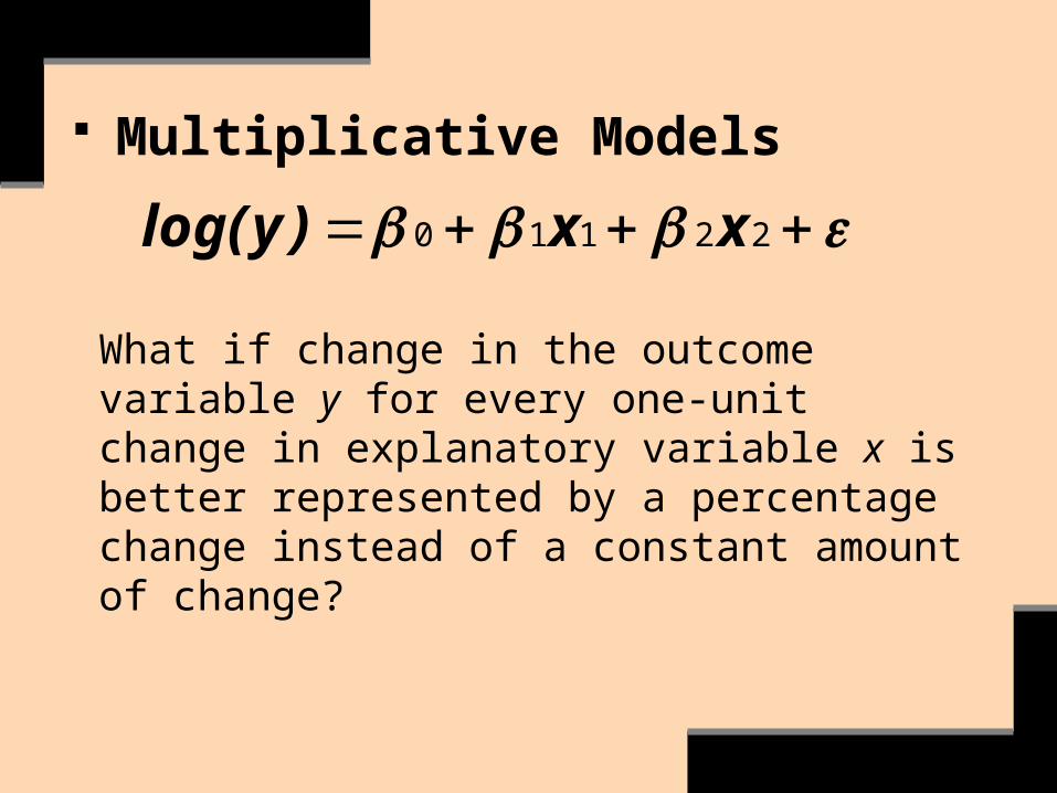
Multiplicative Models
22110 xx)ylog(
What if change in the outcome variable y for every one-unit change in explanatory variable x is better represented by a percentage change instead of a constant amount of change?

The multiplicative (exponential) model is not a linear model, but rather must be transformed into a linear model.
The logarithm model does so.
. use teguc-sya6306, clear

. xi:reg totalconspc i.res_ses hmems sfhh edhhi.res_ses _Ires_ses_1-4 (naturally coded; _Ires_ses_1 omitted)
Number of obs = 1200
Source SS df MS F( 6, 1193) = 176.91
Model 1.0314e+09 6 171906603 Prob > F = 0.0000
Residual 1.1592e+09 1193 971699.592 R-squared = 0.4708
Total 2.1907e+09 1199 1827086.93 j R-squared = 0.4682
Root MSE = 985.75
totalconspc Coef. Std. Err. t P>t [95% Conf. Interval]
_Ires_ses_2 135.2741 76.95551 1.76 0.079 -15.70909 286.2573
_Ires_ses_3 1436.099 83.59843 17.18 0.000 1272.083 1600.115
_Ires_ses_4 1308.239 119.9354 10.91 0.000 1072.931 1543.546
hmems -52.42492 13.30209 -3.94 0.000 -78.52303 -26.32682
sfhh 183.8322 72.37972 2.54 0.011 41.82647 325.8379
edhh 190.7217 19.24278 9.91 0.000 152.9682 228.4751
_cons 324.0004 112.6196 2.88 0.004 103.0459 544.9549

. rvfplot, yline(0)-2
000
02000
4000
6000
Fitte
d v
alu
es
1000 1500 2000 2500 3000Residuals
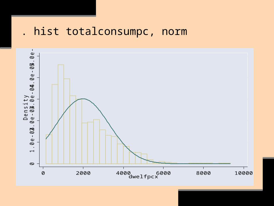
There are problems.

. hist totalconsumpc, norm0
1.0
e-0
42.0
e-0
43.0
e-0
44.0
e-0
45.0
e-0
4D
ensity
0 2000 4000 6000 8000 10000dwelfpcx

. gen ltotalconsumpc=log(totalconsumpc)
. for varlist totalconsumpc ltotalconsumpc: hist X \ more
. su totalconspc ltotalconspc, d
Variable | Obs Mean Std. Dev. Min Max
-------------+--------------------------------------------------------
totalconspc | 1426 1971.418 1321.913 134.917 9341.879
ltotalconspc | 1426 7.3552 .7102317 4.90466 9.142262
. hist totalconsumpc, norm0
1.0
e-0
42.0
e-0
43.0
e-0
44.0
e-0
45.0
e-0
4D
ensity
0 2000 4000 6000 8000 10000dwelfpcx

. hist ltotalconsumpc, norm0
.2.4
.6
Density
5 6 7 8 9ltotalconspc

. xi:reg ltotalconspc i.res_ses hmems sfhh edhh
Source | SS df MS Number of obs = 1200
-------------+------------------------------ F( 6, 1193) = 337.46
Model | 523.538529 6 87.2564215 Prob > F = 0.0000
Residual | 308.472189 1193 .258568473 R-squared = 0.6292
-------------+------------------------------ Adj R-squared = 0.6274
Total | 832.010718 1199 .693920532 Root MSE = .5085
------------------------------------------------------------------------------
ltotalconspc | Coef. Std. Err. t P>|t| [95% Conf. Interval]
-------------+----------------------------------------------------------------
_Ires_ses_2 | .2215539 .0396973 5.58 0.000 .1436695 .2994383
_Ires_ses_3 | .9962171 .0431241 23.10 0.000 .9116096 1.080825
_Ires_ses_4 | .9662357 .0618684 15.62 0.000 .8448526 1.087619
hmems | -.0472669 .0068619 -6.89 0.000 -.0607295 -.0338042
sfhh | .0928064 .0373369 2.49 0.013 .019553 .1660598
edhh | .1472731 .0099263 14.84 0.000 .1277981 .1667482
_cons | 6.116201 .0580946 105.28 0.000 6.002222 6.23018

. rvfplot, yline(0)-3
-2-1
01
2F
itte
d v
alu
es
6.8 7 7.2 7.4 7.6 7.8Residuals
The fit improved.

. xi:reg ltotalconspc i.res_ses hmems sfhh edhh
Source | SS df MS Number of obs = 1200
-------------+------------------------------ F( 6, 1193) = 337.46
Model | 523.538529 6 87.2564215 Prob > F = 0.0000
Residual | 308.472189 1193 .258568473 R-squared = 0.6292
-------------+------------------------------ Adj R-squared = 0.6274
Total | 832.010718 1199 .693920532 Root MSE = .5085
------------------------------------------------------------------------------
ltotalconspc | Coef. Std. Err. t P>|t| [95% Conf. Interval]
-------------+----------------------------------------------------------------
_Ires_ses_2 | .2215539 .0396973 5.58 0.000 .1436695 .2994383
_Ires_ses_3 | .9962171 .0431241 23.10 0.000 .9116096 1.080825
_Ires_ses_4 | .9662357 .0618684 15.62 0.000 .8448526 1.087619
hmems | -.0472669 .0068619 -6.89 0.000 -.0607295 -.0338042
sfhh | .0928064 .0373369 2.49 0.013 .019553 .1660598
edhh | .1472731 .0099263 14.84 0.000 .1277981 .1667482
_cons | 6.116201 .0580946 105.28 0.000 6.002222 6.23018

The log transformation improved the model’s fit.
How do we interpret the log model? (see Wooldrige, pages 46-51, 197-200).

100*[exponent(b) – 1]
. display 100*(exp(-.0473) - 1)= -4.62%
. display 100*(exp(.0928) - 1)= 9.72%
. display 100*(exp(.1473) - 1)= 15.87%
E.g.: for every unit increase in number of household members, household consumption per capita decreases by 4.6% on average, net of the other variables.

Graphing the results is important in interpreting them.
Let’s graph lyhat for ltotalconspc against two of the explanatory variables (hmems & edhh).

. twoway qfitci ltotalconspc hmems, blc(maroon)6.2
6.4
6.6
6.8
77.2
95%
CI/F
itte
d v
alu
es
0 5 10 15# household members
95% CI Fitted values

Next graph: for every unit increase in education (treated as a quantitative-interval variable), consumption increases by 16% on average, holding the other variables constant.

. twoway qfitci ltotalconspc edhh, blc(maroon)6
6.5
77.5
8
95%
CI/F
itte
d v
alu
es
0 2 4 6 8education of household head
95% CI Fitted values

Only quantitative, ratio-level variables with positive values (& ideally a spread of at least 10 units) are eligible for log transformations.
If necessary, transform the original variable as follows to create positive values, e.g.: gen lvar=ln(var + 1)

But don’t use a log transformation if the variable’s original scale contains ‘too many’ zeros (see Wooldridge, page 189; try other models such as ‘poisson’ [see Long & Freese).

What if the outcome variable is ‘level’ (i.e. in the original metric) & an explanatory variable is in log form?
Divide the log-explanatory variable’s coefficient by 100.
For every 1% increase in x (in its original metric), y increases/decreases by … units on average, net of the other variables.

What if both the dependent variable & an explanatory variable are in log form?
Interpretation: for every 1% increase in x (in its original metric), y (in its original metric) increases/decreases by …% on average, holding the other variables constant.

Testing Nested Models

In describing the nature of scientific explanation, Einstein said it should be “as simple as possible, but no simpler” (see also King et al., page 20).
Einstein’s assertion applies to multivariate statistical explanation.
The basic strategy is to comparatively test models in order to select the most parsimonious model that provides the best explanatory, or most predictive, power.
Moreover, a more parsimonious model may have smaller standard errors.

A fundamental approach, then, is to test nested models.
Two models are nested if one model contains all the terms of the second model & at least one additional term.
. use hsb2, clear
.xi:reg science read write math female white i.prog socst schtyp
.xi:reg science read write math female white
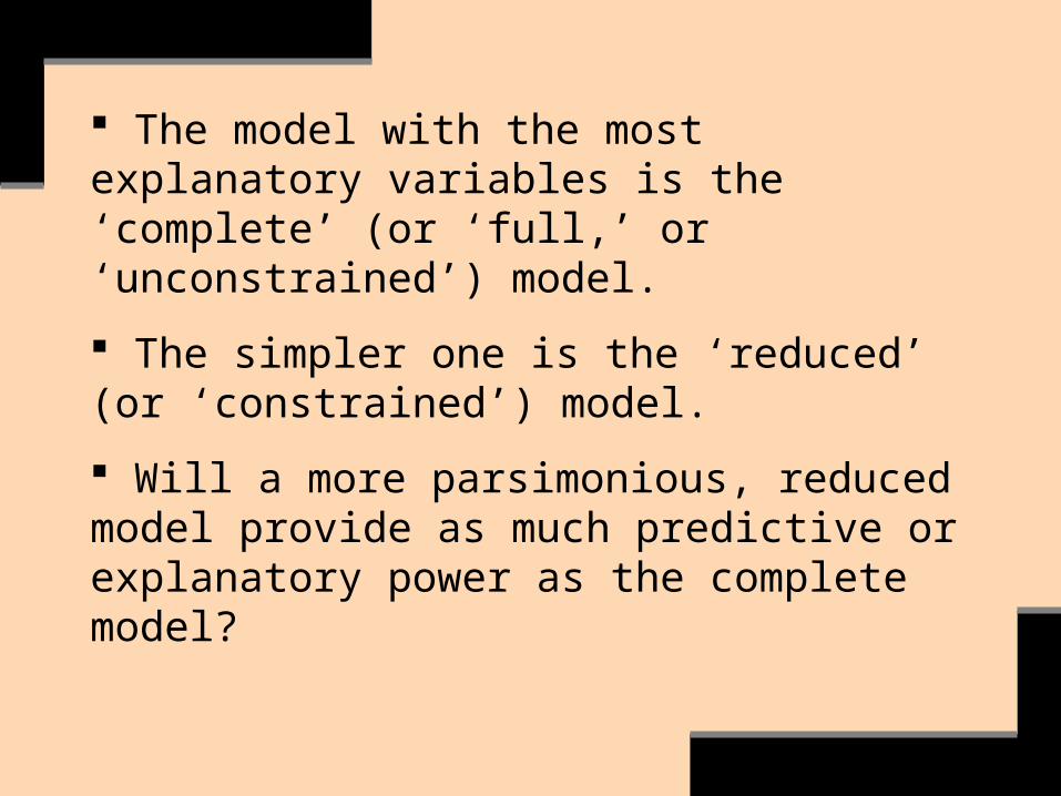
The model with the most explanatory variables is the ‘complete’ (or ‘full,’ or ‘unconstrained’) model.
The simpler one is the ‘reduced’ (or ‘constrained’) model.
Will a more parsimonious, reduced model provide as much predictive or explanatory power as the complete model?

The comparative test of nested models is conducted by testing the null hypothesis that the full model’s additional variables equal zero, versus the alternative hypothesis that at least one of the full model’s additional variables is different from zero:
0
0
54
54
k
k
,, ofone least at :Ha
:Ho

We comparatively test the nested models via the ‘F test for comparing nested models’ (sometimes called the ‘partial F test’).
The test compares the SSEC with the SSER by calculating the difference: if the complete model’s extra explanatory variables are jointly significant, then the SSEC should be much smaller than SSER, & thus the difference SSEC- SSER will be large.
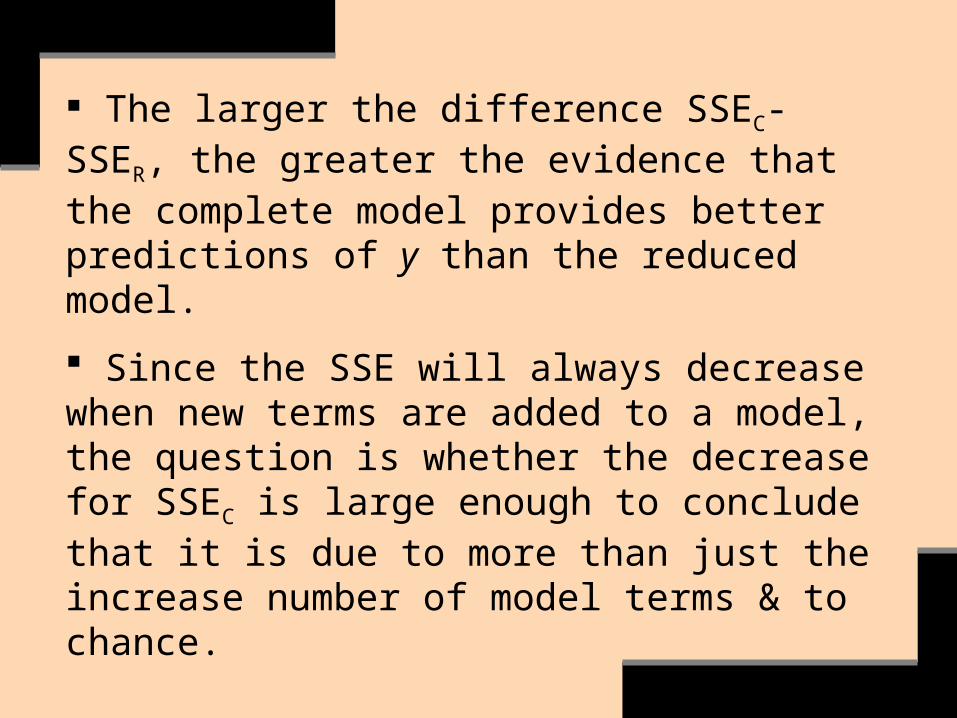
The larger the difference SSEC- SSER, the greater the evidence that the complete model provides better predictions of y than the reduced model.
Since the SSE will always decrease when new terms are added to a model, the question is whether the decrease for SSEC is large enough to conclude that it is due to more than just the increase number of model terms & to chance.

1)](k-[nSSE
g)-)/(kSSE-(SSEF
C
CR
C
CR
MSE
tested s'/#SSESSE(
F F:region Rejection #observations must be equal

STATA makes testing nested models (i.e. the F test for comparing nested models) easy:
Estimate the full regression model.
Using the command test, conduct a hypothesis test on the full model’s explanatory variables that aren’t included in the reduced model.
If the extra explanatory variables test jointly significant, reject Ho & keep the full model; if they test jointly insignificant, fail to reject Ho & select the reduced model.

For a valid test of nested models:
(1) The number of observations in both models must be equal.
(2) The functional form of the outcome variable must be the same (e.g., there’s no comparing a raw-form y with a log-transformed y).
(3) The functional form of the nested models must be the same (both must be, e.g., OLS).

To ensure that the nested models have the same number of observations, use STATA’s mark/markout commands to make a ‘complete’ binary variable:

. mark complete
. markout complete science read write math female ses race
. tab complete
. reg science read write math if complete==1
. xi:reg science read write math i.female i.ses i.race if complete==1
‘complete’ is the new variable’s name.

. test _Ifemale_1 _Ises_2 _Ises_3 _Irace_2 _Irace_3 _Irace_4
( 1) _Ifemale_1 = 0
( 2) _Ises_2 = 0
( 3) _Ises_3 = 0
( 4) _Irace_2 = 0
( 5) _Irace_3 = 0
( 6) _Irace_4 = 0
F( 6, 190) = 4.85
Prob > F = 0.0001
Or: . testparm _Ifemale_1 -_Irace_4

Note that variables may test insignificant individually but significant jointly. E.g., let’s say that we added the variables ‘prog’ to ‘schtyp’ to a model:
. xi:reg science read write math female white i.prog schtyp
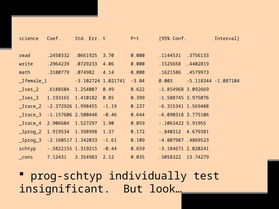
science Coef. Std. Err. t P>t [95% Conf. Interval]
read .2450332 .0661925 3.70 0.000 .1144531 .3756133
write .2964239 .0729233 4.06 0.000 .1525658 .4402819
math .3100779 .074982 4.14 0.000 .1621586 .4579973
_Ifemale_1 -3.102724 1.021741 -3.04 0.003 -5.118344 -1.087104
_Ises_2 .6188504 1.254007 0.49 0.622 -1.854968 3.092669
_Ises_3 1.193165 1.410182 0.85 0.399 -1.588745 3.975076
_Irace_2 -2.372926 1.998455 -1.19 0.237 -6.315341 1.569488
_Irace_3 -1.157606 2.500448 -0.46 0.644 -6.090318 3.775106
_Irace_4 2.906604 1.527297 1.90 0.059 -.1063422 5.91955
_Iprog_2 1.919534 1.398998 1.37 0.172 -.840312 4.679381
_Iprog_3 -2.160517 1.342033 -1.61 0.109 -4.807987 .4869523
schtyp -.5822155 1.319215 -0.44 0.659 -3.184671 2.020241
_cons 7.12431 3.354983 2.12 0.035 .5058322 13.74279
prog-schtyp individually test insignificant. But look…

Check their correlations for possible insight (see Wooldrige, pages 157-58).
. test _Iprog_2 _Iprog_3 schtyp
( 1) _Iprog_2 = 0
( 2) _Iprog_3 = 0
( 3) schtyp = 0
F( 3, 187) = 3.72
Prob > F = 0.0125
They test jointly significant.

Conclusion: Reject Ho in favor of the complete model, because the added variables test jointly significant.
See Wooldrige (page 158) on the challenges of dealing with the combination of joint insignificance & individual significance.

Here’s a way to test non-nested models via Bayesian statistics.
The approach of Bayesian statistics is to assess the ‘relative plausibility’ of models in view of a sample’s data.
Download ‘fitstat’ (see Long/ Freese).

. use hsb2, clear
. reg math science read write
. fitstat, saving(m1)
. reg math science read socst
. fitstat, using(m1) bic [using, not saving]
The results will indicate ‘relative strength’ of support for model 2 versus model 1.

To summarize, we use a six-step procedure to create a regression model:
(1) Hypothesize the form of the model for E(y).
(2) Collect the sample data.
(3) Use the sample data to estimate unknown parameters in the model.

(4) Specify the probability distribution of the random error term, & estimate any unknown parameters of this distribution.
(5) Statistically check the usefulness of the model.
(6) When satisfied that the model is useful, use it for prediction, estimation, & so on.

Fundamental Principles Always have sound conceptual reasons for selecting variables & the forms of their relationships with the outcome variable.
Graph & write the reasons for your choices, including relative to the alternatives (i.e. rival hypotheses).
Always be skeptical. Ask ‘What kind of evidence would force me to revise or reject my model?’ (see King et al. & Ragin).