Ignoring Interprocessor Communication During Scheduling

Portland State University Portland State University

PDXScholar PDXScholar

Dissertations and Theses Dissertations and Theses

1992

Ignoring Interprocessor Communication During Ignoring Interprocessor Communication During

Scheduling Scheduling

Chintamani M. Patwardhan Portland State University

Follow this and additional works at: https://pdxscholar.library.pdx.edu/open_access_etds

Part of the Computer Engineering Commons, and the Electrical and Computer Engineering Commons

Let us know how access to this document benefits you.

Recommended Citation Recommended Citation Patwardhan, Chintamani M., "Ignoring Interprocessor Communication During Scheduling" (1992). Dissertations and Theses. Paper 4422. https://doi.org/10.15760/etd.6300

This Thesis is brought to you for free and open access. It has been accepted for inclusion in Dissertations and Theses by an authorized administrator of PDXScholar. Please contact us if we can make this document more accessible: [email protected].

https://pdxscholar.library.pdx.edu/

https://pdxscholar.library.pdx.edu/open_access_etds

https://pdxscholar.library.pdx.edu/etds

https://pdxscholar.library.pdx.edu/open_access_etds?utm_source=pdxscholar.library.pdx.edu%2Fopen_access_etds%2F4422&utm_medium=PDF&utm_campaign=PDFCoverPages

http://network.bepress.com/hgg/discipline/258?utm_source=pdxscholar.library.pdx.edu%2Fopen_access_etds%2F4422&utm_medium=PDF&utm_campaign=PDFCoverPages

http://network.bepress.com/hgg/discipline/266?utm_source=pdxscholar.library.pdx.edu%2Fopen_access_etds%2F4422&utm_medium=PDF&utm_campaign=PDFCoverPages

http://library.pdx.edu/services/pdxscholar-services/pdxscholar-feedback/

https://doi.org/10.15760/etd.6300

mailto:[email protected]

IGNORING INTERPROCESSOR COMMUNICATION

DURING SCHEDULING

by

CHINT AMANI M. PA TW ARD HAN

A thesis submitted in partial fulfillment of the requirements for the degree of

MASTER OF SCIENCE in

ELECTRICAL AND COMPUTER ENGINEERING

Portland State University

1992

AN ABSTRACT OF THE THESIS OF Chintamani M. Patwardhan for the Master of

Science in Electrical and Computer Engineering presented December 13, 1991.

Title: Ignoring Interprocessor Communication During Scheduling.

APPROVED BY THE MEMBERS OF THE THESIS COMMITTEE:

Michael A. Driscolr, Chair

W. ~obert Daasch

The goal of parallel processing is to achieve high speed computing by partitioning

a program into concurrent parts, assigning them in an efficient way to the available pro-

cessors, scheduling the program and then executing the concurrent parts simultane-

ously. In the past researchers have combined the allocation of tasks in a program and

scheduling of those tasks into one operation. We define scheduling as a process of

efficiently assigning priorities to the already allocated tasks in a program. Assignment

of priorities is important in cases when more than one task at a processor is ready for

execution. Most heuristics for scheduling consider certain parameters of the architec-

2

ture and the program. These parameters could be the execution time of each operation

in a program, the number of processors, etc. The impact of ignoring interprocessor

communication (IPC) when ordering parallel tasks has, however, not been well studied.

We develop a model of the impact of ignoring IPC for parallel programs using

barrier synchronization, when scheduled by a critical path algorithm. The model allows

us to prove a theorem that identifies the cases for which IPC is important. For those

cases, our model and experiments show that a program scheduled ignoring IPC per

forms almost as well as a program scheduled using IPC. Since including interprocessor

communication in scheduling is expensive, we conclude that, for our programs and

scheduling algorithm, it is reasonable to ignore IPC while scheduling.

TO THE OFFICE OF GRADUATE STUDIES:

The members of the Committee approve the thesis of Chintamani M. Patwardhan

presented December 13, 1991.

Micha"el A. Driscoll, Chair

APPROVED:

Rolf Schaumann, Chair, Department of Electrical Engineering

C. William Savery, Vice Provost for Graduate Stu naResearch

ACKNOWLEDGEMENTS

Researching and writing a MS thesis is a lengthy process. During my academic

life at PSU many people have provided assistance through financial and moral support.

The most significant person, of course, has been my advisor, Dr. Michael Driscoll. I am

grateful to him for giving me advice on courses, thesis topics, research pointers and in

writing this document.

I would also like to thank other members of the ParPlum project: Jingsong Fu,

De-Zheng Tang, Kiswanto Thayib, Satish Pai and Liono Setiowijoso for their support,

co-operation and the hilarious moments we shared together.

I wish to thank the School of Business Administration and Dr. Beverley Fuller for

the financial support.

Finally, thanks to my mother Mrs. Sheelaprabha Patwardhan and my brother Dr.

Gagan Patwardhan for their financial and moral support during my entire academic life.

Without their encouragement and support I probably would have never made it.

Chintamani M. Patwardhan

TABLE OF CONTENTS

PAGE

ACKNOWLEDGEMENTS............................................ iii

LIST OFT ABLES . . . . . . . . . . . . . . . . . . . . . . . . . . . . . . . . . . . . . . . . . . . . . . . . . . . vi

LIST OF FIGURES . . . . . . . . . . . . . . . . . . . . . . . . . . . . . . . . . . . . . . . . . . . . . . . . . . vii

NOTATIONS AND GLOSSARY....................................... ix

CHAPTER

I INTRODUCTION ...................................... .

1.1 Problem Statement . . . . . . . . . . . . . . . . . . . . . . . . . . . . . . . 1

1.2 Motivation and Purpose of this Research . . . . . . . . . . . . . . 2

1.3 Thesis Overview . . . . . . . . . . . . . . . . . . . . . . . . . . . . . . . . . 3

II OVERVIEW OF SCHEDULING METHODS . . . . . . . . . . . . . . . . . 5

2.1 Background . . . . . . . . . . . . . . . . . . . . . .. . . . . . . . . . . . . . . 5

2.2 Classification of Scheduling Algorithms....... . . . . . . . 6

2.3 Scheduling Algorithms and their Properties . . . . . . . . . . . . 8

2.4 Scheduling Definition Function and Goal . . . . . . . . . . . . . 11

III PARALLEL PROGRAMS AND THEIR INFLUENCE

ON GLOBAL SCHEDULES.................. . . . . . . . . . . . . 16

3.1 Importance of Parallel Paths for Global Schedule . . . . . . 16

3.2 Suitable Scheduling Algorithms......... . . . . . . . . . . . 19

3.3 Importance of A Cut in A Path. . . . . . . . . . . . . . . . . . . . . 20

3.4 Experimental Focus . . . . . . . . . . . . . . . . . . . . . . . . . . . . . 25

IV MODELING SCHEDULE EXECUTION TIMES . . . . . . . . . . . . . 26

v

4.1 An Ideal Graph . . . . . . . . . . . . . . . . . . . . . . . . . . . . . . . . . . 26

4.2 Modeling Approach . . . . . . . . . . . . . . . . . . . . . . . . . . . . . . 27

4.3 Graph Behavior versus Variations in Key Parameters.... 30

4.4 Behavioral Prediction of Experimental Outcome... . . . . 36

V EXPERIMENTAL RESULTS AND THEIR ANALYSIS........ 37

5.1 Variation in Paths 1 and 2 (Path 3 Constant ) . . . . . . . . . . 37

5.2 Variation in Path 3 (Path 1 and 2 Constant).. . . . . . . . . 42

5.3 Variation in Path 1 (Path 2 and 3 Constant).. . . . . . . . . 46

5.4 Variation in Path 2 (Path 1 and 3 Constant)... . . . . . . . 49

5.5 Model Performance Analysis . . . . . . . . . . . . . . . . . . . . . . 52

VI CONCLUSION . . . . . . . . . . . . . . . . . . . . . . . . . . . . . . . . . . . . . . . . . 53

6.1 Significance of this Research . . . . . . . . . . . . . . . . . . . . . . . 53

6.2 Future Work.................................... 54

REFERENCES . . . . . . . . . . . . . . . . . . . . . . . . . . . . . . . . . . . . . . . . . . . . . . . . . . . . . 57

LIST OF TABLES ..,

TABLE PAGE

I Schedule for Graph in Figure 8 . . . . . . . . . . . . . . . . . . . . . . . . . . . . . . . . . 28

II Execution Time for Graphs with Path 1and2 Varying Simultaneously.. 39

III Execution Time for Graphs with Path 3 Varying (Global Schedule) . . . . 43

IV Execution Time for Graphs with Path 3 Varying (Local Schedule) . . . . . 44

V Execution Time for Graphs with Path 1 Varying (Global Schedule).... 47

VI Execution Time for Graphs with Path 1 Varying (Local Schedule)...... 47

VII Execution Time for Graphs with Path 2 Varying (Global Schedule) . . . . . 50

VIII Execution Time for Graphs with Path 2 Varying (Local Schedule)...... 50

IX Schedule for Fine Grain . . . . . . . . . . . . . . . . . . . . . . . . . . . . . . . . . . . . . . . 55

LIST OF FIGURES

FIGURE

1 A Graph depicting the Importance of Scheduling .................. .

2 Assignment of Priorities When Graph in Figure 1 is

Scheduled Globally and Locally ............................... .

3 A General Parallel Program ................................... .

4 A Parallel Program with Paths Assigned to Processors .............. .

5 Firing Sequence of Paths in Figure 4 When Scheduled

PAGE

12

14

16

18

by Granski 's Heuristic . . . . . . . . . . . . . . . . . . . . . . . . . . . . . . . . . . . . . . . . 20

6 Graph with Uncut Parallel Strings Allocated to two Processors . . . . . . . . . . 21

7 Mapping Pieces of a Cut Path to different Processors . . . . . . . . . . . . . . . . . 22

8 An Ideal Graph for Modeling Execution time of

Global and Local Schedules . . . . . . . . . . . . . . . . . . . . . . . . . . . . . . . . . . . . . 26

9 Dataflow Graph in Figure 8 Modeled as a Set of Paths

between Fork and Join Points......... . . . . . . . . . . . . . . . . . . . . . . . . . . 27

10 Execution Sequence of nodes in Figure 8 for Global Schedule . . . . . . . . . . 29

11 Execution Sequence of nodes in Figure 8 for Local Schedule . . . . . . . . . . 29

12 General Execution Sequence for Globally Scheduled Graph in Figure 8... 31

13 General Execution Sequence for Locally Scheduled Graph in Figure 8 . . . . 31

14 Graph of Variation in number of Nodes in Path 1 and 2

Versus total Execution time of Globally and Locally Scheduled graph.... 40

15 Graph of Variation in Number of Nodes in Path 1 and 2

Versus Difference in total Execution time........ . . . . . . . . . . . . . . . . . 40

viii

16 Child Execution time for Globally and Locally Scheduled

Graph in Figure 8 . . . . . . . . . . . . . . . . . . . . . . . . . . . . . . . . . . . . . . . . . . . . 41

17 Variation in IPC............................................ 42

18 Graph for Variation in Number of Nodes on Path 3

Nodes on Paths 1 & 2 = 200 . . . . . . . . . . . . . . . . . . . . . . . . . . . . . . . . . . . 44


Nodes on Paths 1 & 2 = 100................................... 45


Nodes on Paths 1 & 2 = 50 . . . . . . . . . . . . . . . . . . . . . . . . . . . . . . . . .. . . 45


Nodes on Paths 2 & 3 = 10................................ . . . 48


Nodes on Path 2 = 50 & Path 3 = 10 . . . . . . . . . . . . . . . . . . . . . . . . . . . . . 48


Nodes on Path 2 = 100 & Path 3 = 10......... . . . . . . . . . . . . . . . . . . 49


Nodes on Path 1 = 50 & Path 3 = 10 . . . . . . . . . . . . . . . . . . . . . . . . . . . . 51


Nodes on Path 1=100 & Path 3 = 10........................... 51

26 A Comparison of Global and Local Scheduler Execution times . . . . . . . . . 52

27 An example of Fine and Coarse Grain Scheduling . . . . . . . . . . . . . . . . . . . 54

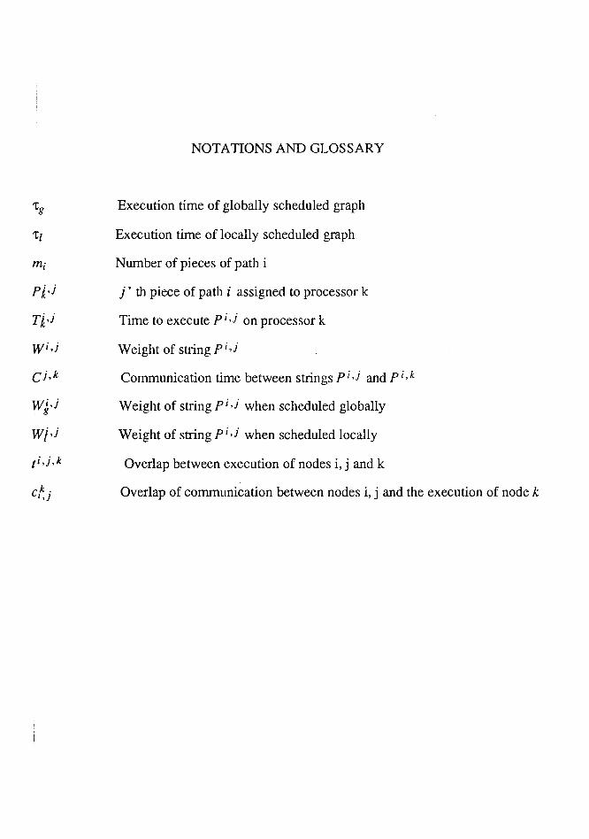
NOTATIONS AND GLOSSARY

'tg Execution time of globally scheduled graph

't1 Execution time of locally scheduled graph

mi Number of pieces of path i

Pi, j j ' th piece of path i assigned to processor k

Ti·j Time to execute pi,j on processor k

Wi,j WeightofstringPi,j

C j, k Communication time between strings Pi ,j and Pi· k

~k,j Weight of string pi,j when scheduled globally

Wi·j Weight of string pi,j when scheduled locally

ti ,j, k Overlap between execution of nodes i, j and k

cf.j Overlap of communication between nodes i, j and the execution of node k

CHAPTER I

INTRODUCTION

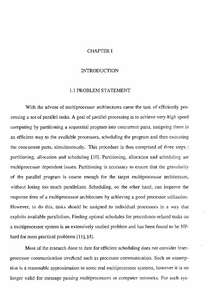
1.1 PROBLEM ST A TEMENT

With the advent of multiprocessor architectures came the task of efficiently pro

cessing a set of parallel tasks. A goal of parallel processing is to achieve very-high speed

computing by partitioning a sequential program into concurrent parts, assigning them in

an efficient way to the available processors, scheduling the program and then executing

the concurrent parts, simultaneously. This procedure is thus comprised of three steps :

partitioning, allocation and scheduling (10]. Partitioning, allocation and scheduling are

multiprocessor dependent issues. Partitioning is necessary to ensure that the granularity

of the parallel program is coarse enough for the target multiprocessor architecture,

without losing too much parallelism. Scheduling, on the other hand, can improve the

response time of a multiprocessor architecture by achieving a good processor utilization.

However, to do this, tasks should be assigned to individual processors in a way that

exploits available parallelism. Finding optimal schedules for precedence-related tasks on

a multiprocessor system is an extensively studied problem and has been found to be NP

hard for most practical problems [11], [4].

Most of the research done to date for efficient scheduling does not consider inter

processor communication overhead such as processor communication. Such an assump

tion is a reasonable approximation to some real multiprocessor systems, however it is no

longer valid for message passing multiprocessors or computer networks. For such sys-

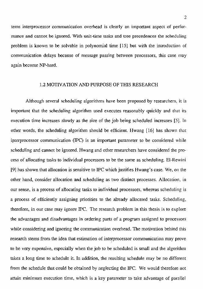
2

terns interprocessor communication overhead is clearly an important aspect of perfor

mance and cannot be ignored. With unit-time tasks and tree precedences the scheduling

problem is known to be solvable in polynomial time [15] but with the introduction of

communication delays because of message passing between processors, this case may

again become NP-hard.

1.2 MOTIVATION AND PURPOSE OF THIS RESEARCH

Although several scheduling algorithms have been proposed by researchers, it is

important that the scheduling algorithm used executes reasonably quickly and that its

execution time increases slowly as the size of the job being scheduled increases [5]. In

other words, the scheduling algorithm should be efficient. Hwang [16] has shown that

ipterprocessor communication (IPC) is an important parameter to be considered while

scheduling and cannot be ignored. Hwang and other researchers have considered the pro

cess of allocating tasks to individual processors to be the same as scheduling. El-Rewini

[9] has shown that allocation is sensitive to IPC which justifies Hwang's case. We, on the

other hand, consider allocation and scheduling as two distinct processes. Allocation, in

our sense, is a process of allocating tasks to individual processors, whereas scheduling is

a process of efficiently assigning priorities to the already allocated tasks. Scheduling,

therefore, in our case may ignore IPC. The research problem in this thesis is to explore

the advantages and disadvantages in ordering parts of a program assigned to processors

while considering and ignoring the communication overhead. The motivation behind this

research stems from the idea that estimation of interprocessor communication may prove

to be very expensive, especially when the job to be scheduled is small and the algorithm

takes a long time to schedule it. In addition, the resulting schedule may be no different

from the schedule that could be obtained by neglecting the IPC. We would therefore not

attain minimum execution time, which is a key parameter to take advantage of parallel

3

processing.

Since many algorithms have been suggested by various researchers for efficient

scheduling, we will focus on the following objectives in this thesis:

1. Identifying the scheduling algorithms suitable for our research.

2. Identifying graphs and their properties that show a difference in assignment of

priorities and execution time while considering and ignoring the IPC.

3. Designing a simple dataftow graph and models predicting its performance under

the situation cited above.

4. Experimental testing of the model graph on the ParPlum interpreter [10].

5. Evaluating the results obtained from experiments.

It is our hypothesis that for some programs and scheduling algorithms, operations

at a processor can be ordered without regard to the interprocessor communication time.

1.3 THESIS OVERVIEW

Chapter II begins with an overview of research carried out for efficient scheduling

of graphs, the definitions of global and local scheduling, and their importance. Chapter

III tries to find the properties of mappings that show a difference in global and local

schedules. To do so, it presents possible mappings of a graph on an architecture and tne

effect of global and local schedules on the execution time of such mappings . Chapter IV

begins by showing a graph designed for experiments, which has the properties needed to

see a difference in assig~ment of priorities using global and local schedules and later

presents models that can predict the performance of the experimental graph. Chapter V

presents the results of executing the model graph on the ParPlum interpreter after apply

ing the global and local scheduling techniques to it. A comparison of the experimental

results with the results predicted by the models is also analyzed. Finally, Chapter VI

4

presents conclusions, reviews the usefulness of the research presented herein, and points

out directions for future research.

CHAPTER II

OVERVIEW OF SCHEDULING METHODS

2.1 BACKGROUND

Processor scheduling has a long history of study. Early research on the scheduling

problem concentrated on the scheduling of work in job shops. Later, researchers investi

gated the problem of scheduling jobs on uniprocessor systems using multitasking operat

ing systems [33]. However, with the arrival of multiprocessing systems came the task of

scheduling the jobs on them so as to minimize the parallel execution time of a job and to

better utilize the processors in the system. An efficient scheduling algorithm should allo

cate a set of tasks to the available processors of a multiprocessor system and determine

the sequence or order of execution of the tasks allocated to each member processor. Most

of the scheduling problems suggested to date are NP-Hard [ 4], [11]. Some algorithms

may usually have low computational requirements, but become enumerative under cer

tain circumstances. Even most of the relaxed and simplified subproblems, derived from

the original scheduling problems by adding restrictions to them, fall into the class of

NP-Hard problems [4]. The restrictions usually added are:

1. Preemption not allowed;

2. The number of parallel processors used;

3. Attributes of tasks such as topology of the task graph; and

4. Uniformity of task processing times.

6

Some scheduling problems can be solved in polynomial time (24]. For example,

when the task graph is a tree and the execution time of all the tasks is one time unit, Hu

[ 15] showed that by using a list scheduling algorithm an optimal solution can be found in

O(n) time. Hu' s algorithm assigns a level number to each node in the task graph on the

basis of the length of the longest path from the node to an exit node of the precedence

graph. In a second case when the precedence relation is arbitrary but the number of pro

cessors is limited to two, Coffman & Graham [4] showed that by using a list scheduling

algorithm similar to Hu, a solution can be reached in O(n 2) time. The two special prob

lems mentioned above, however, become NP-Hard [4] if any one restricting condition is

relaxed. To circumvent these problems, heuristic algorithms have been proposed to

obtain approximate or suboptimal solutions to such problems in polynomial time.

2.2 CLASSIFICATION OF SCHEDULING ALGORITHMS

While various scheduling problems have been studied for years, a detailed survey

of earlier results presented by Gonzalez [11] describes a scheme by which the scheduling

problems can be classified. His criteria takes into consideration the following:

1. The type of precedence among tasks in the program;

2. The type of processors used in the architecture; and

3. The number of processors in the architecture.

The tasks in the program may have arbitrary precedence or no precedence at all,

the architecture may have any number of processors and the processors themselves could

l;>e homogeneous or heterogenous. Kruatrachue [22], on the other hand, suggests that the

results in parallel processor scheduling can be classified into five classes on the basis of

the goal of the scheduler, the type of task to be scheduled and the parallel processor sys

tem. The groups in turn would be as follows:

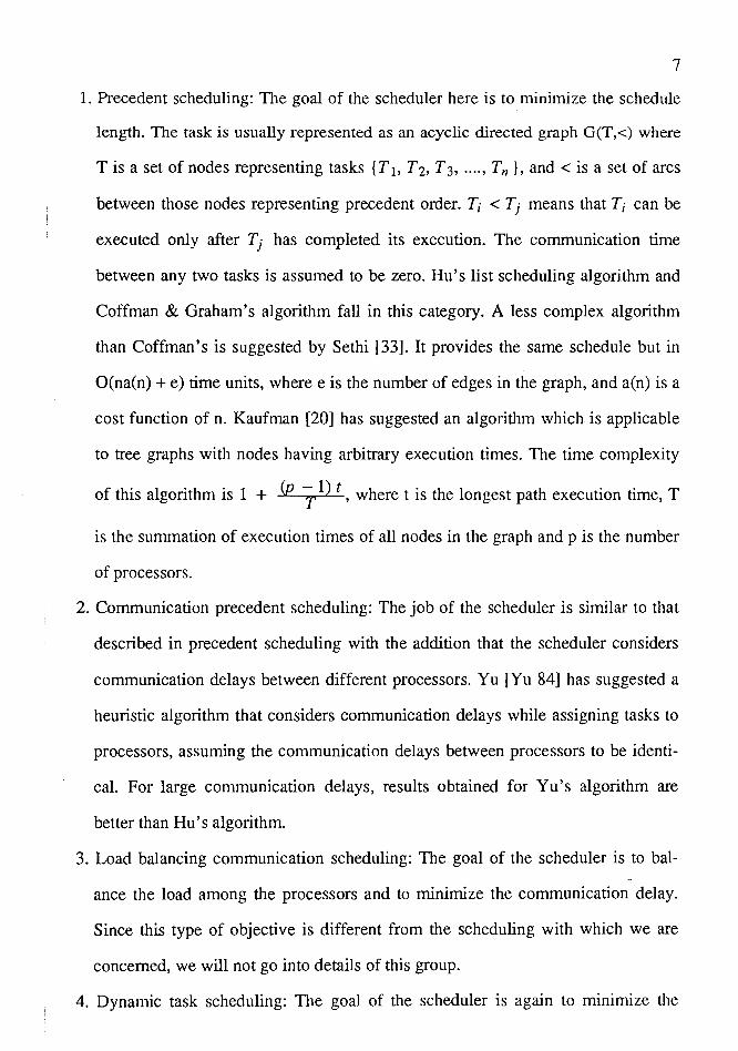
7

1. Precedent scheduling: The goal of the scheduler here is to minimize the schedule

length. The task is usually represented as an acyclic directed graph G(T,<) where

Tis a set of nodes representing tasks {Ti, Tz, T3, .... , Tn }, and< is a set of arcs

between those nodes representing precedent order. T; < Tj means that T; can be

executed only after Tj has completed its execution. The communication time

between any two tasks is assumed to be zero. Hu's list scheduling algorithm and

Coffman & Graham's algorithm fall in this category. A less complex algorithm

than Coffman's is suggested by Sethi [33]. It provides the same schedule but in

O(na(n) + e) time units, where e is the number of edges in the graph, and a(n) is a

cost function of n. Kaufman [20] has suggested an algorithm which is applicable

to tree graphs with nodes having arbitrary execution times. The time complexity

of this algorithm is 1 + (p Tl) t, where tis the longest path execution time, T

is the summation of execution times of all nodes in the graph and p is the number

of processors.

2. Communication precedent scheduling: The job of the scheduler is similar to that

described in precedent scheduling with the addition that the scheduler considers

communication delays between different processors. Yu [Yu 84] has suggested a

heuristic algorithm that considers communication delays while assigning tasks to

processors, assuming the communication delays between processors to be identi

cal. For large communication delays, results obtained for Yu's algorithm are

better than Hu's algorithm.

3. Load balancing communication scheduling: The goal of the scheduler is to bal

ance the load among the processors and to minimize the communication delay.

Since this type of objective is different from the scheduling with which we are

concerned, we will not go into details of this group.

4. Dynamic task scheduling: The goal of the scheduler is again to minimize the

8

schedule length. Here, however, the node execution times, the communication

time between processors, the number of nodes in the graph and the precedent con

straint are varying and can be changed during execution. Graphs with loop or

branching statements usually fall into this category since the number of iterations

of a loop may not be known beforehand. Ramamoorthy [30] and Kund [23] have

proposed a heuristic for dynamic scheduling in which the schedule is determined

at runtime. These complex schedule strategies however, introduce excessive over

head in this case and there is no guarantee of near optimal schedules.

5. Independent task scheduling: The goal of the scheduler is to improve the load

balancing and meeting the individual task deadlines.

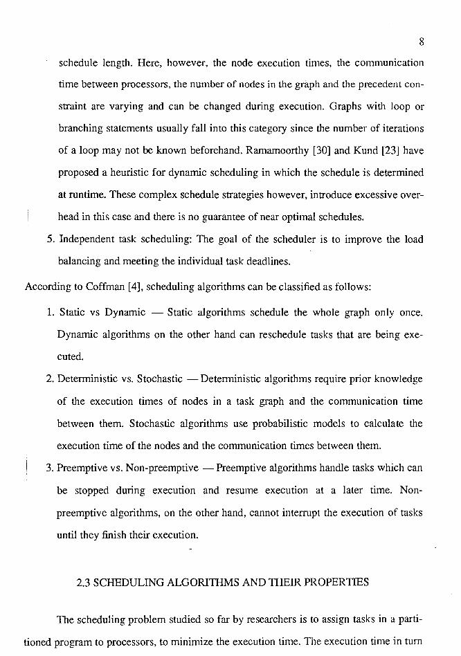
According to Coffman [ 4], scheduling algorithms can be classified as follows:

1. Static vs Dynamic - Static algorithms schedule the whole graph only once.

Dynamic algorithms on the other hand can reschedule tasks that are being exe

cuted.

2. Deterministic vs. Stochastic - Deterministic algorithms require prior knowledge

of the execution times of nodes in a task graph and the communication time

between them. Stochastic algorithms use probabilistic models to calculate the

execution time of the nodes and the communication times between them.

3. Preemptive vs. Non-preemptive - Preemptive algorithms handle tasks which can

be stopped during execution and resume execution at a later time. Non

preemptive algorithms, on the other hand, cannot interrupt the execution of tasks

until they finish their execution.

2.3 SCHEDULING ALGORITHMS AND THEIR PROPERTIES

The scheduling problem studied so far by researchers is to assign tasks in a parti

tioned program to processors, to minimize the execution time. The execution time in turn

9 ' depends on processor utilization and on the overhead incurred in interprocessor commun-

ication. From the theoretical standpoint there are two types of scheduling disciplines 1)

general and 2) list [25]. A general schedule usually describes the exact initiation time of

the tasks and so it requires the execution time of the tasks to be deterministic. To ensure

the shortest execution time of the schedule generated, some of the processors may remain

idle, waiting for some important tasks to get ready for execution, even though some other

tasks are already waiting to be executed [29]. While general scheduling has many

shortcomings when applied in practice, where perfect synchronization is impossible, it

still serves as the best one can do to optimize execution in a static sense. List scheduling,

on the other hand, is simply a priority list of the tasks involved, and no processor is left

idle during execution. The list schedule is an effective and realistic technique in practice !

and is applicable even if the task execution times vary greatly from one another [25].

Another important fact is that if the execution time of all the tasks are the same, then

there is no distinction between an optimal list schedule and an optimal general schedule.

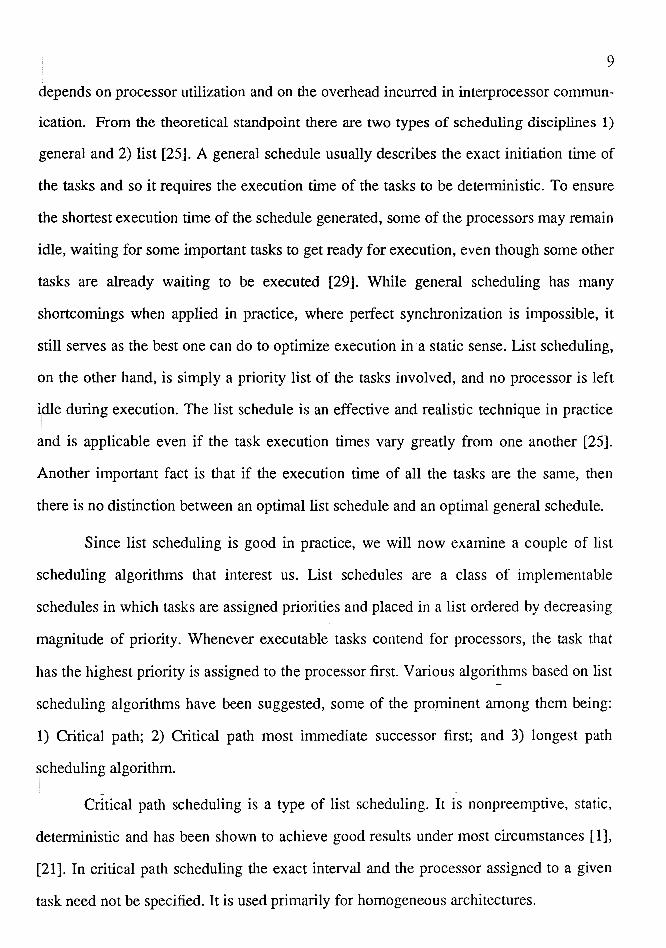
Since list scheduling is good in practice, we will now examine a couple of list

scheduling algorithms that interest us. List schedules are a class of implementable

schedules in which tasks are assigned priorities and placed in a list ordered by decreasing

magnitude of priority. Whenever executable tasks contend for processors, the task that

has the highest priority is assigned to the processor first. Various algorithms based on list

scheduling algorithms have been suggested, some of the prominent among them being:

1) Critical path; 2) Critical path most immediate successor first; and 3) longest path

scheduling algorithm. !

Critical path scheduling is a type of list scheduling. It is nonpreemptive, static,

deterministic and has been shown to achieve good results under most circumstances [l],

[21]. In critical path scheduling the exact interval and the processor assigned to a given

task need not be specified. It is used primarily for homogeneous architectures.

10

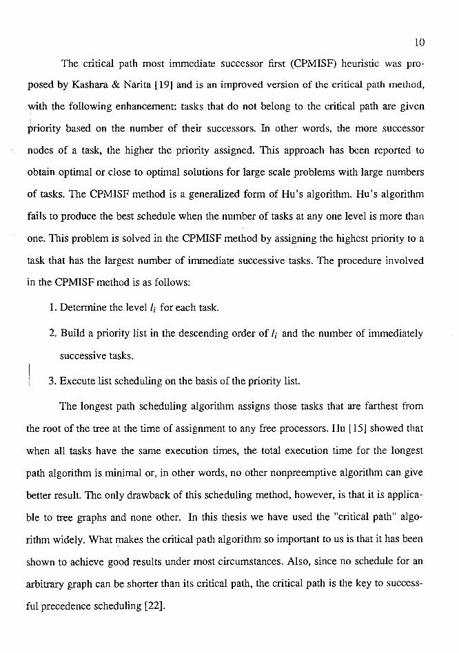
The critical path most immediate successor first (CPMISF) heuristic was pro

posed by Kashara & Narita [19] and is an improved version of the critical path method,

with the following enhancement: tasks that do not belong to the critical path are given

priority based on the number of their successors. In other words, the more successor

nodes of a task, the higher the priority assigned. This approach has been reported to

obtain optimal or close to optimal solutions for large scale problems with large numbers

of tasks. The CPMISF method is a generalized form of Hu's algorithm. Hu's algorithm

fails to produce the best schedule when the number of tasks at any one level is more than

one. This problem is solved in the CPMISF method by assigning the highest priority to a

task that has the largest number of immediate successive tasks. The procedure involved

in the CPMISF method is as follows:

1. Determine the level I; for each task.

2. Build a priority list in the descending order of I; and the number of immediately

successive tasks.

3. Execute list scheduling on the basis of the priority list.

The longest path scheduling algorithm assigns those tasks that are farthest from

the root of the tree at the time of assignment to any free processors. Hu [15] showed that

when all tasks have the same execution times, the total execution time for the longest

path algorithm is minimal or, in other words, no other nonpreemptive algorithm can give

better result. The only drawback of this scheduling method, however, is that it is applica

ble to tree graphs and none other. In this thesis we have used the "critical path" algo

rithm widely. What makes the critical path algorithm so important to us is that it has been

shown to achieve good results under most circumstances. Also, since no schedule for an

arbitrary graph can be shorter than its critical path, the critical path is the key to success

ful precedence scheduling [22].

11

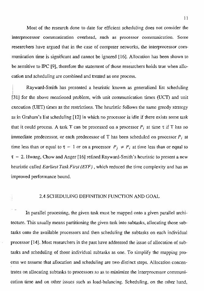
Most of the research done to date for efficient scheduling does not consider the

interprocessor communication overhead, such as processor communication. Some

researchers have argued that in the case of computer networks, the interprocessor com

munication time is significant and cannot be ignored [16]. Allocation has been shown to

be sensitive to IPC [9], therefore the statement of those researchers holds true when allo

cation and scheduling are combined and treated as one process.

Rayward-Smith has presented a heuristic known as generalized list scheduling

[31] for the above mentioned problem, with unit communication times (UCT) and unit

execution (UET) times as the restrictions. The heuristic follows the same greedy strategy

as in Graham's list scheduling [12] in which no processor is idle if there exists some task

that it could process. A task T can be processed on a processor P; at time 'C if T has no

immediate predecessor, or each predecessor of T has been scheduled on processor P; at

time less than or equal to 'C - 1 or on a processor Pj -:/:- P; at time less than or equal to

't - 2. Hwang, Chow and Anger [16] refined Rayward-Smith's heuristic to present a new

heuristic called Earliest Task First (ETF), which reduced the time complexity and has an

improved performance bound.

2.4 SCHEDULING DEFINITION FUNCTION AND GOAL

In parallel processing, the given task must be mapped onto a given parallel archi

tecture. This usually means partitioning the given task into subtasks, allocating those sub

tasks onto the available processors and then scheduling the subtasks on each individual

processor [14]. Most researchers in the past have addressed the issue of allocation of sub

tasks and scheduling of those individual subtasks as one. To simplify the mapping pro

cess we assume that allocation and scheduling are two distinct steps. Allocation concen

trates on allocating subtasks to processors so as to minimize the interprocessor communi

cation time and on other issues such as load-balancing. Scheduling, on the other hand,

12

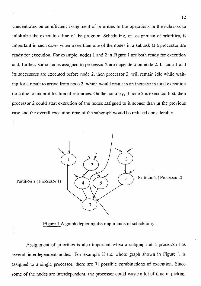
concentrates on an efficient assignment of priorities to the operations in the subtasks to

minimize the execution time of the program. Scheduling, or assignment of priorities, is

important in such cases when more than one of the nodes in a subtask at a processor are

ready for execution. For example, nodes 1 and 2 in Figure 1 are both ready for execution

and, further, some nodes assigned to processor 2 are dependent on node 2. If node 1 and

its successors are executed before node 2, then processor 2 will remain idle while wait

ing for a result to arrive from node 2, which would result in an increase in total execution

time due to underutilization of resources. On the contrary, if node 2 is executed first, then

processor 2 could start execution of the nodes assigned to it sooner than in the previous

case and the overall execution time of the subgraph would be reduced considerably.

Partition 1 (Processor 1) Partition 2 (Processor 2)

Figure 1.A graph depicting the importance of scheduling.

Assignment of priorities is also important when a subgraph at a processor has

several interdependent nodes. For example if the whole graph shown in Figure 1 is

assigned to a single processor, there are 7! possible combinations of execution. Since

some of the nodes are interdependent, the processor could waste a lot of time in picking

13

up a node for execution and then finding that its predecessor has not been executed yet.

If, however, the nodes are first assigned priorities and the processor then executes the

nodes on the basis of their priorities, the overhead would be greatly reduced. '

Figure 1 further clarifies the difference between our definition of scheduling and

that proposed by other researchers. In our scheduling a processor has access to only a

subgraph and its nodes for execution. On the contrary, the literature published by other

researchers suggests that once partitioned, nodes in a subgraph which are ready for exe-

cution can be assigned/scheduled to any of the processors that are free for work.

A scheduler, in our sense, is an algorithm that takes as input a partitioned and

allocated task graph and produces as output a priority list of operations in the task graph.

An optimal schedule results when the scheduler generates a list of tasks that guarantees

the shortest execution time. A scheduling algorithm should execute quickly and its exe-

cution time should increase slowly when the task size increases. It makes little sense to

tise a scheduler that takes a long time to schedule a job that takes only a small time to

execute. Granski [13] seconds this opinion by suggesting that incorporating the schedul-

ing mechanism in a computer is an expensive proposition.

Most of the heuristics for list scheduling explained in section 2.3 consider some

parameters of the architecture or the task graph itself. These parameters could include the

execution time of each node in the task graph, the number of processors in the architec-

ture and the critical path of the node to be scheduled. It is our hypothesis that the order-

ing of operations at processors can be done without regard to the interprocessor commun-

ication. To evaluate this hypothesis we will have to look into some possible ways of

mapping a program to processors and then single out those which could show a differ

ence in assigned priorities and execution time under the influence of IPC. To aid further

research we define two scheduling methods: I

1. Global Schedule : Ordering the whole graph while considering the

·.r 14

communication (or dependencies) between processors.

2. Local Schedule : Ordering the individual subgraphs allocated to each processor

while ignoring any communication arcs between the processors.

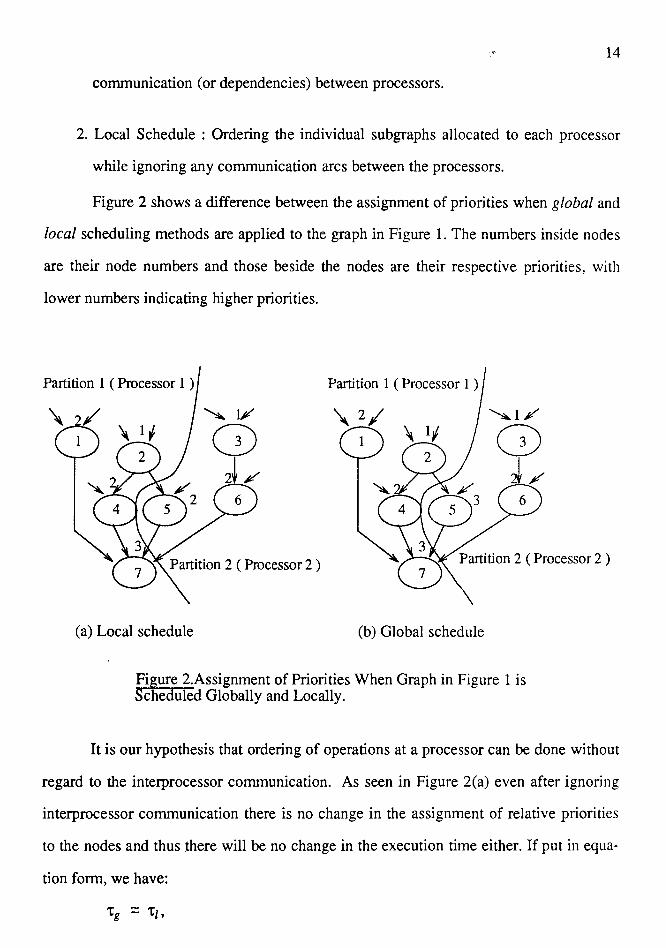
Figure 2 shows a difference between the assignment of priorities when global and

local scheduling methods are applied to the graph in Figure 1. The numbers inside nodes

are their node numbers and those beside the nodes are their respective priorities, with

lower numbers indicating higher priorities.

Partition 1 ( Processor 1 ) Partition 1 ( Processor 1 )

(a) Local schedule (b) Global schedule

Fi ure 2.Assignment of Priorities When Graph in Figure 1 is cheduled Globally and Locally.

It is our hypothesis that ordering of operations at a processor can be done without

regard to the interprocessor communication. As seen in Figure 2(a) even after ignoring

interprocessor communication there is no change in the assignment of relative priorities

to the nodes and thus there will be no change in the execution time either. If put in equa-

tion form, we have:

'tg ::: 't/ '

15

'tg ;:::; 'tz,

where 'tg and 'tz represent the execution time of globally and locally scheduled graphs.

Also, since the global scheduler considers the interprocessor communication time, its

computational complexity will always be greater than or equal to the local scheduler, i.e.,

0 ( g ) 2 0 (/ ).

CHAPTER III

PARALLEL PROGRAMS AND THEIR INFLUENCE

ON GLOBAL SCHEDULES

3.1 IMPORTANCE OF PARALLEL PATHS FOR GLOBAL SCHEDULE

Partitioning, allocating and scheduling tasks for execution on a computer system

requires the mapping of the tasks to the computer system hardware in a manner that

improves some aspect of system performance. Scheduling thrives on parallelism present

~n algorithms. A parallel program therefore has to be mapped to an architecture

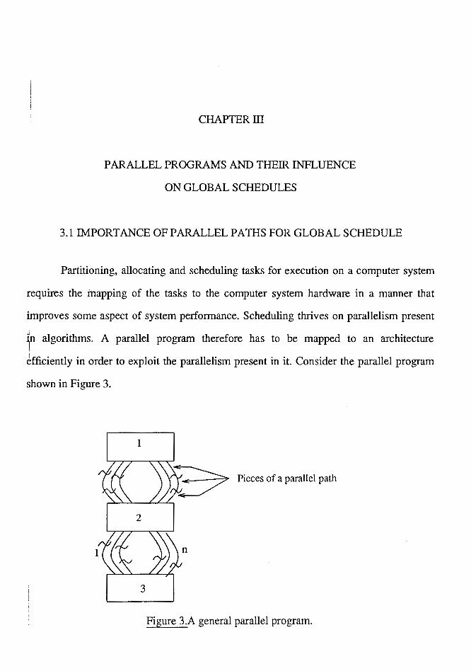
6fficiently in order to exploit the parallelism present in it. Consider the parallel program

shown in Figure 3.

1

E7 Pieces of a parallel path

3

Figure 3.A general parallel program.

17

The rectangular blocks represent fork and join points of the program. A fork

point, by definition, has two or more independent paths leading out of it and execution

must proceed along each and every one of the paths leading out of the fork. Their com-

mon output point is called a join point. In Figure 3 blocks 1 and 3 represent fork and join

J?Oints, respectively, and block 2 represents both. Each block in such a case would I represent a barrier [34] in the execution sequence of the program or, in other words, the

program would stop and then start its parallel execution at each block. A barrier is a con-

venient synchronization mechanism among executing processes. The synchronization

requires that all processes execute the barrier construct before any process can proceed

past it to the next executable statement. Barriers are usually used to satisfy a number of

data dependences simultaneously by imposing sequentiality on the production and use of

the data items. In the Force language [17], a section of code is inserted between the

beginning and end of a barrier construct. This code is executed by one processor after all

processes arrive at the barrier and before any process leaves it. Similarly blocks 1 and 3

in Figure 3 could be the startup and ending code, respectively, of a program. This simple

model may be extended to a well defined form of concurrent processing which is

~epresented by nodes (instructions) on paths between a pair of fork and join points. Each

path in such a case would represent a subtask of the entire program. In fact, barrier syn

chronization is commonly used in many parallel programming applications [18].

To clarify the analysis further let us define the components of Figure 3. Note that

in the discussion that follows we will use path to mean a chain or string of operations in a

graph. A path starts at a fork point and ends at a join point. If generalized, the model

shown 1n Figure 3 can be represented as having n parallel paths. During the mapping

process the graph would be partitioned and then allocated. During the partitioning phase,

depending on the partitioning algorithm being used, the subtasks or paths could be

clustered and assigned to the same or different processors and an individual path may be

cut (split) into pieces. Applying this terminology to the parallel program shown in

18

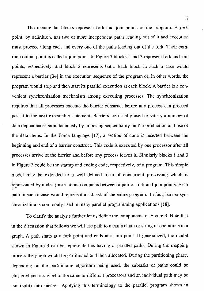
Figure 3, let m; represent the number of pieces of path i and pki ,j represent the j 'th

piece of path i assigned to processor Pk, where

l~i~n

1 ~j ~i·

Figure 4 shows a parallel program annotated using this terminology.

path 2

p I

1 I

I

J

BEGIN

I I I I

P' i

I _J

~_i I - Pf·l

ut in path 4

r Pf·2

END I m 1 = m 2 = m 3 = m 5 = 1 , m 4 = 2

Figure 4.A parallel program with paths assigned to processors.

The multiprocessor architecture model to which parallel programs are mapped

donsists of a number of homogeneous or heterogeneous processors. The processors com

municate via an interconnection network and the amount of time taken to send a fixed

amount of data from one processor to another is constant. Each processor in the architec-

ture contains only one arithmetic-logic unit. Computations at processors and communica-

tion between them may proceed in parallel subject to the dependency constraints of the

algorithm.

19

3.2 SUITABLE SCHEDULING ALGORITHMS

As described in Chapter II we found that the list scheduling heuristic suggested

by Granski [13] is appropriate to finding a suitable model depicting a difference in global

and local schedules. Granski's heuristic is based on the critical path algorithm and incor

porates a development by which graphs with conditional nodes and loops can be

scheduled. The latter case, however, is possible only when the number of iterations of a

loop in the graph is known prior to execution. In such cases the loop can be unrolled to

produce an acyclic graph, which is then scheduled. The heuristic starts by first assigning

1eights to all of the strings of nodes in the paths of the graph, where the weight of a

string is the sum of the execution times of all nodes in it and the maximum weight of its

successor strings. In order to assign weights the algorithm starts with each string Pi· m;

connected to the join point of a program, assigns it a weight and then assigns weights to

strings whose successor strings have already been assigned weights. So if Pi· k is a string

which is a successor of string Pi· i and T Jn· i is the time to execute Pi· i on processor m ,

then the weight of Pi ,j can be written as:

w i, j = Ti, j + . kmax ( w i. k ) m pi, E SUCC (1)

where W i • i is the weight of string Pi ,j

While mapping a graph to a multiprocessor system the graph may be partitioned

~d hence a string in a subgraph could have a predecessor string in another subgraph. In

such cases we have to consider the communication time between strings and the equation

for the weight of a string would then be:

Wi,j = Ti,j + . kmax (Wi,k + Ci,k) (2) m pi, E SUCC

where Ci,k is the communication time between strings pi.j and pi,k.

Once all strings have been assigned weights, they are assigned priorities in

decreasing order of their weights. In situations where two or more strings have the same

20

weights, a string having the longest path length from it to the exit node is assigned the

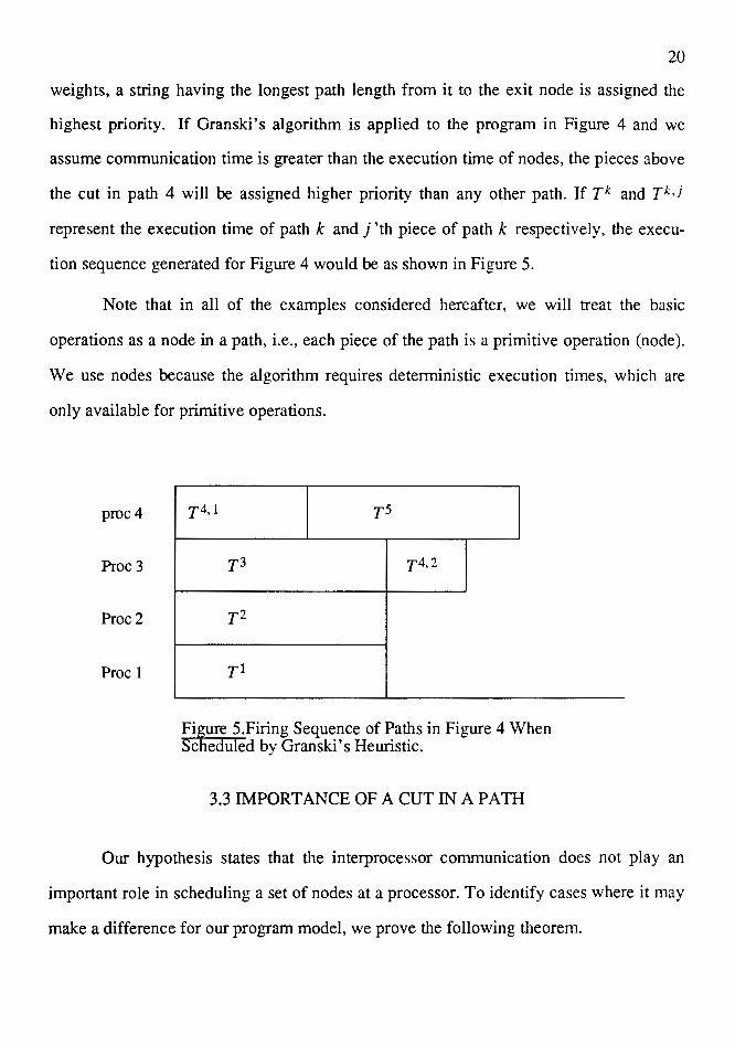
highest priority. If Granski's algorithm is applied to the program in Figure 4 and we

assume communication time is greater than the execution time of nodes, the pieces above

the cut in path 4 will be assigned higher priority than any other path. If Tk and Tk,j

represent the execution time of path k and j 'th piece of path k respectively, the execu

tion sequence generated for Figure 4 would be as shown in Figure 5.

Note that in all of the examples considered hereafter, we will treat the basic

operations as a node in a path, i.e., each piece of the path is a primitive operation (node).

We use nodes because the algorithm requires deterministic execution times, which are

only available for primitive operations.

proc4

Proc 3

Proc2

Proc 1

T4,I Ts

T3 T4,2

T1

TI

Fi ure 5.Firing Sequence of Paths in Figure 4 When cheduled by Gran ski's Heuristic.

3.3 IMPORTANCE OF A CUT IN A PATH

Our hypothesis states that the interprocessor communication does not play an

important role in scheduling a set of nodes at a processor. To identify cases where it may

make a difference for our program model, we prove the following theorem.

21

Theorem

Assignment of relative priorities changes only if a path in a program is cut.

To prove this theorem we have to investigate all possible mappings of a program

to an architecture and look for any change in the assignment of priorities and execution '

!me because of interprocessor communication. Note that if relative priorities remain I

unchanged, execution time will also remain unchanged.

Proof

We analyze two cases of mappings, one in which none of the paths are cut and the

second in which one of the paths is cut. We will then study the assignment of priorities to

the strings of nodes in each allocation in the global and local schedule cases. Note that

path Pk·j has higher priority than Pl·m if and only if Wi,j - wt,m ~ 0, where Wi,j is

the weight of the j 'th piece of path i.

P4

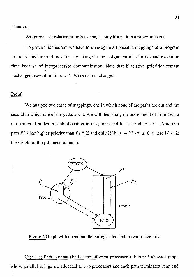
Figure 6.Graph with uncut parallel strings allocated to two processors.

Case 1.a) Path is uncut (End at the different processors). Figure 6 shows a graph

whose parallel strings are allocated to two processors and each path terminates at an end

22

node residing in processor 2. First consider two arbitrary paths P 1 and P 2 at processor 1.

Using the notation shown in section 3.2 and global schedule, piece i of path P 1 has

weight Wg1·i = ~ yl,k + C, i.e, the sum of execution times of the successor paths plus k =i

the communication to the end node. Similarly the weight of piece j of path P 2 for global

schedule will be Wj·i = 2. y2,k + C. k =1

The priority of piece PI, i is higher than P 2,j if and only if Wgl. i - Wj·i ;:::: 0.

If we substitute the weights of path P 1 and P 2 in above condition, we get:

~ yl,k + c - ! y2,k - c ;:::: 0 k=i k=j

or

~ yl,k - ! y2,k ;:::: 0. k=i k=j

The local scheduler does not consider the communication time, so the piece i of path P 1

and piece j of path P 2 will have weights as follows.

w11,i = ~ yl,k k = i

w12,j = ! y2,k k =j

Since there is no relative difference in the local weights of P 1. i and P 2· J and

since the amount of communication between paths P 1 and P 2 with the end node is the

same, we can therefore conclude that Wi· i - Wg2-i ;:::: 0 if and only if

W11·i - W12.i ;:::: 0, and the relative priorities under global and local schedules are identi-

9al.

Case l.b) Path is uncut (End at the same processors). In Figure 6 paths P 3 and P 4

and the end node have been assigned to the same processor. The global weights of paths

P 1 and P 2 do not change from the global to the local schedule because there is no com-

23

munication with the end node and so neither has a higher priority than the other.

3

Proc 2

Proc 1

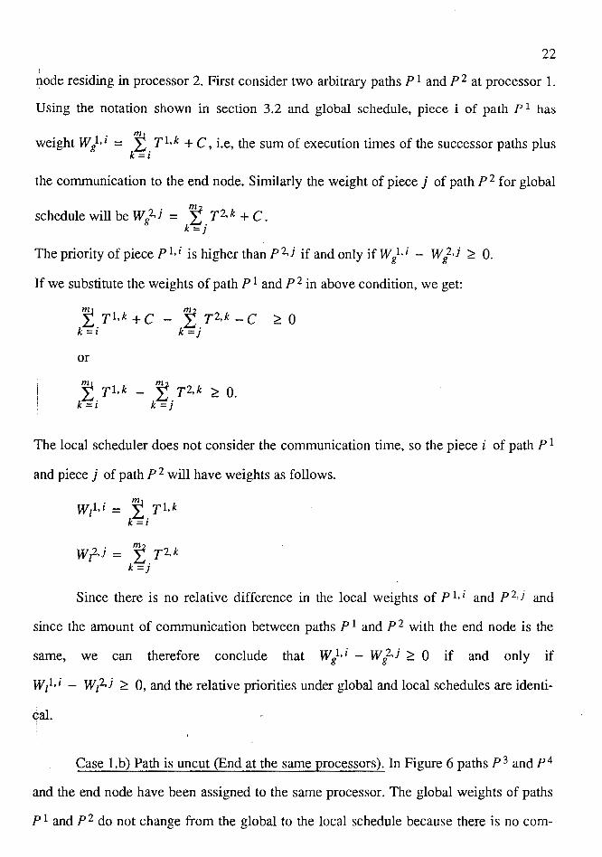
Figure 7 .Mapping pieces of a cut path to different processors.

Case 2.a) Path is cut. We will analyze a case in which pieces of a cut path will be

assigned to different processors. Figure 7 shows such a mapping. On the basis of the I notation developed in section 3.1, the equations for the weights of paths P 1 and p2 under

global scheduling can be written as:

ForpieceiofuncutpathPl: W/i = ~ yl,k k =i

For piece j of cut path 2: Wg2·j = ~ y2, k + n C k =j

where n is the number of cuts in path 2 and piece j is above the cut.

In the case of the local schedule the weight of piece i of path P 1 will be the same as glo

bal weight but the weight of piece j of path P 2 will be

w12,j = ~ y2,k k=j

where m 2 < m 2 and is the number of nodes above the cut. In the global schedule case,

the relative priority of piece i of path 1 will higher than that of piece j of path 2 if and

I 24

I

only if Wi· i - W/·j :2:0

Substituting the global weights for piece i and j we get:

~ r1.k _ r r2.k _ n c ;:::: o IC=i k=j

Now consider the case when ~ yl,k IC= i

= L y2, k. The equation for global weights k=j

will then be:

' r r2.k - r r2.k - n c ;:::: o IC=j IC=j

or

~ y2,k ;:::: r y2,k + n c k=j li=j

I This case is true only if n C < 0. Communication time, however, is always greater than

0 and so r y2,k + n c is always greater than r y2,k. In other words piece j of path k=j k=j

P 2 will have higher priority than piece i of path P 1. In the local schedule case, the rela

tive priority of piece i of path 1 will higher than that of piece j of path 2 if and only if

W11,; - Wz2,j ~

Substituting the local weights for piece i and j we get:

~ yl.k _ r y2.k ;;:: o k=i k=j

In such a case when the lengths of piece i of path 1 and piece j of path 2 are same, their

weights will be same. In other words, in the local schedule case, piece i of path 1 will

lave higher priority than piece j of path 2 which is different than the global schedule.

We can therefore conclude that the relative priorities in global and local schedule cases

are different when a path is cut, proving the theorem.

25

3.4 EXPERIMENT AL FOCUS

As seen from the above explanations, a major difference in global and local

Jchedule execution times occurs only when a path is cut into multiple pieces. To show I

our hypothesis, we must now look at the importance of the difference when a path is cut

and its effect on the execution time. This analysis will be based on a simple dataftow

graph model to be shown in Chapter IV. This model, though being a very specific map-

ping case, has two parallel paths, one of which is cut into two pieces. Since a cut in a

path is all that makes a difference in execution time, the model should be sufficient in

designing our experiments. Communication time between processors is a major factor

which brings out a difference in execution time when a path is cut. We will vary the

number of nodes that reside on the pieces of paths and observe the effect of their overlap

with the communication time on the execution of globally and locally scheduled graphs.

CHAPTER IV

MODELING SCHEDULE EXECUTION TIMES

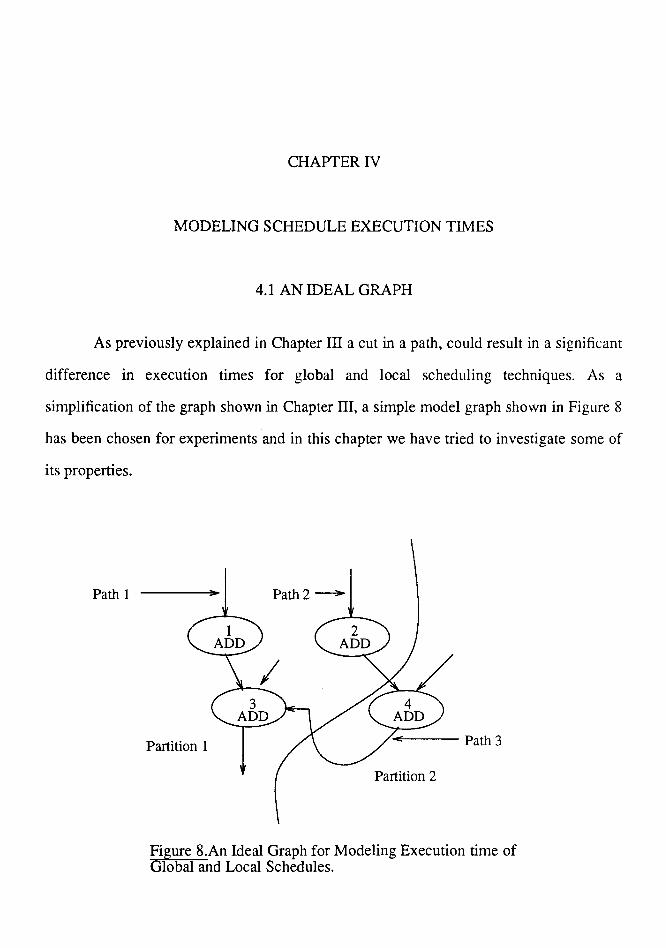
4.1 AN IDEAL GRAPH

As previously explained in Chapter III a cut in a path, could result in a significant

difference in execution times for global and local scheduling techniques. As a

simplification of the graph shown in Chapter III, a simple model graph shown in Figure 8

has been chosen for experiments and in this chapter we have tried to investigate some of

its properties.

Path 1 Path2 __..,.

Partition 1 / Path 3

Partition 2

Figure 8.An Ideal Graph for Modeling Execution time of Global and Local Schedules.

27

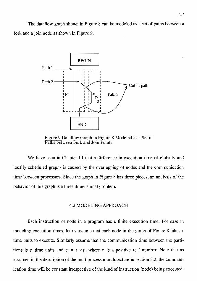
The dataflow graph shown in Figure 8 can be modeled as a set of paths between a

fork and a join node as shown in Figure 9.

BEGIN

Path 1 r - - -1- -T , r - - - , I I I

Path 2 ---:---+--

I

•P : 1 I I I

L - - -•-

I I I

END

P' 2: I I

.J

Figure 9.Dataflow Graph in Figure 8 Modeled as a Set of Paths between Fork and Join Points.

We have seen in Chapter III that a difference in execution time of globally and

locally schedul~d graphs is caused by the overlapping of nodes and the communication

time between processors. Since the graph in Figure 8 has three pieces, an analysis of the

behavior of this graph is a three dimensional problem.

4.2 MODELING APPROACH

Each instruction or node in a program has a finite execution time. For ease in

modeling execution times, let us assume that each node in the graph of Figure 8 takes t

time units to execute. Similarly assume that the communication time between the parti-

tions is c time units and c = z x t, where z is a positive real number. Note that as

assumed in the description of the multiprocessor architecture in section 3.2, the commun-

ication time will be constant irrespective of the kind of instruction (node) being executed.

28

communication time will be constant irrespective of the kind of instruction (node) being

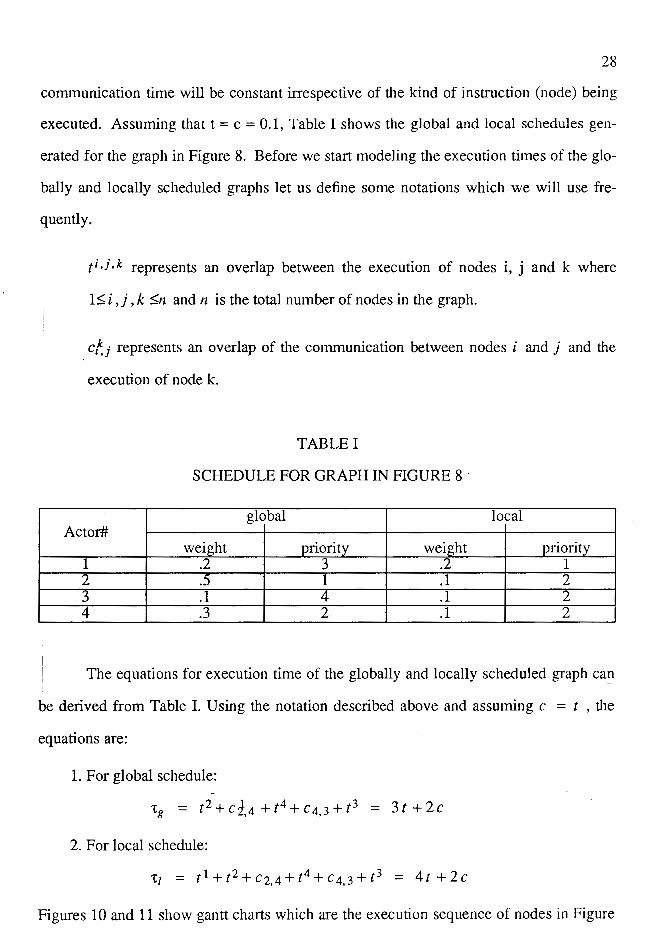
executed. Assuming that t = c = 0.1, Table I shows the global and local schedules gen

erated for the graph in Figure 8. Before we start modeling the execution times of the glo

bally and locally scheduled graphs let us define some notations which we will use fre-

quently.

ti ,j • k represents an overlap between the execution of nodes i, j and k where

1~ i, j, k ~ and n is the total number of nodes in the graph.

cf.i represents an overlap of the communication between nodes i and j and the

execution of node k.

TABLE I

SCHEDULE FOR GRAPH IN FIGURE 8

global local Actor#

weight priority weight priority 1 .2 3 .2 1 2 .5 1 .1 2 3 .1 4 .1 2 4 .3 2 .1 2

The equations for execution time of the globally and locally scheduled graph ca~

be derived from Table I. Using the notation described above and assuming c = t , the

equations are:

1. For global schedule:

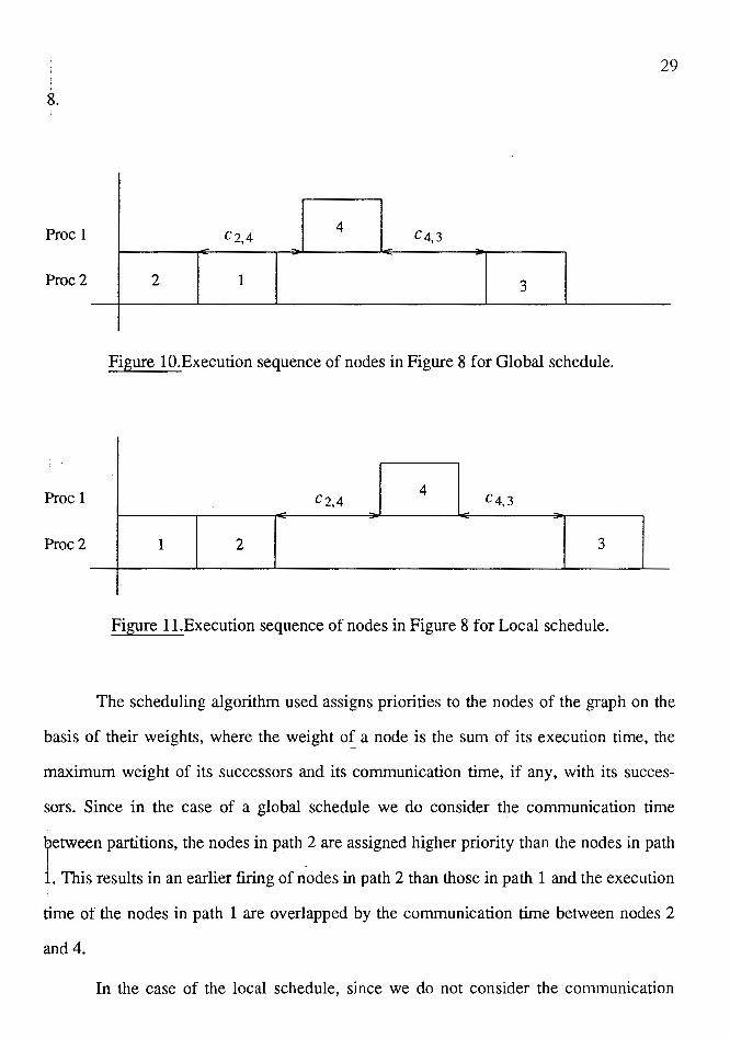
'tg = t2+c1,4+t4+c4,3+t3 = 3t+2c

2. For local schedule:

't/ = t 1+t2+c2,4+t4+c4,3+t3 = 4t +2c

Figures 10 and 11 show gantt charts which are the execution sequence of nodes in Figure

29

8.

Proc 1 Cz,4 4

C4,3 - :;; ::: :;;

Proc2 2 1 3

Figure IO.Execution sequence of nodes in Figure 8 for Global schedule.

I -Proc 1 Cz,4

4 C4,3

-

Proc2 1 2 3

Figure 11.Execution sequence of nodes in Figure 8 for Local schedule.

The scheduling algorithm used assigns priorities to the nodes of the graph on the

basis of their weights, where the weight of a node is the sum of its execution time, the

maximum weight of its successors and its communication time, if any, with its succes-

sors. Since in the case of a global schedule we do consider the communication time

letween partitions, the nodes in path _2 are assigned higher priority than the nodes in path

1. This results in an earlier firing of nodes in path 2 than those in path 1 and the execution

time of the nodes in path 1 are overlapped by the communication time between nodes 2

and4.

In the case of the local schedule, since we do not consider the communication

30

between the partitions, the nodes in path 1 and path 2 are assigned priorities in an alter-

nating fashion. This results in node 1 firing before node 2 and no overlap of nodes occurs

with the communication between node 2 and node 4. As seen from the above interpreta-1

ti.on the key parameters which bring out different schedules and different execution times ! '

are:

1. The communication time between the allocations.

2. Length of paths 1, 2 and 3.

3. The execution time of the nodes in the graph.

4. Scheduling algorithms used.

If this is put in an equation form, we have:

T = t1 - 'tg = f (list scheduling , t, c ,path lengths )

Since the graph's behavior depends on the number of nodes in paths 1 and 2 and

also on the number of nodes in path 3, an analysis of the behavior will be a three dimen

~ional problem. In the following sections we will analyse the behavior of the graph for

varying the number of nodes in paths 1, 2 and 3.

4.3 GRAPH BEHAVIOR VERSUS VARIATIONS IN KEY PARAMETERS

To ease an understanding of the analysis that will follow we will first put forward

some naming conventions:

1. nP 1 = the number of nodes in path 1.

2. nµ2 =the number of nodes in path 2.

3. np3 = the number of nodes in path 3.

4. r =the number of arcs between the two partitions.

As suggested in section 4.2 the difference in execution time of globally and

locally scheduled graphs is a function of the lengths of paths 1, 2 and 3. To predict the

31

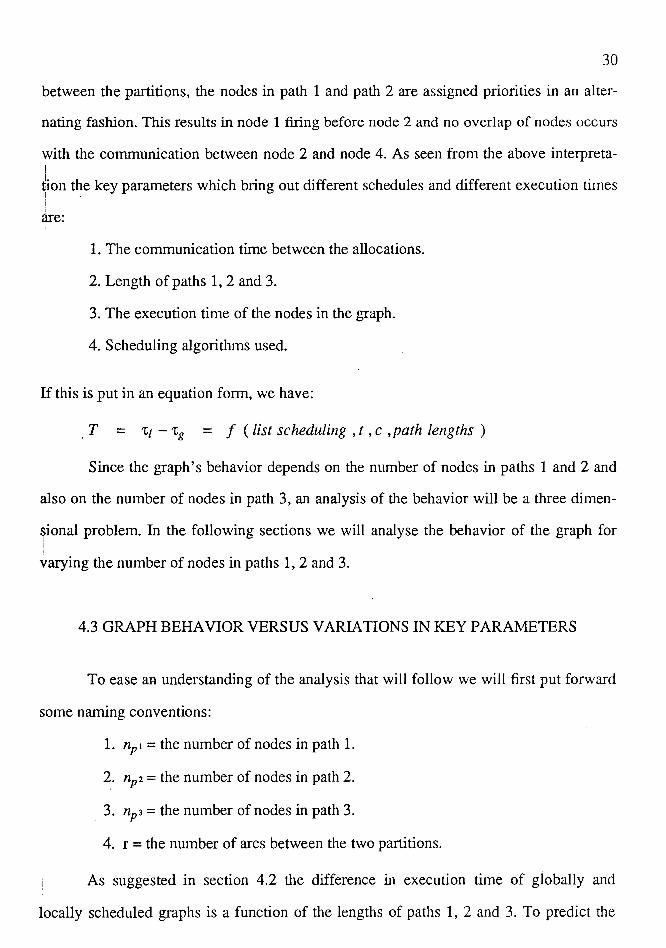
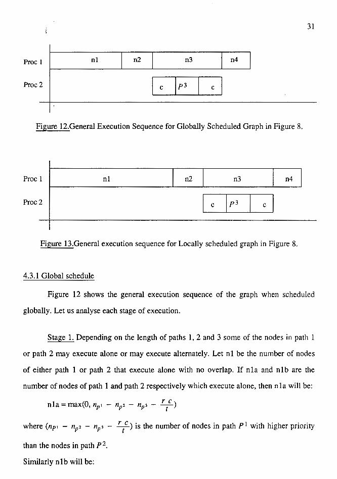
Proc 1 nl n2 n3 n4

Proc2 I c IP 3 I c I

Figure 12.General Execution Sequence for Globally Scheduled Graph in Figure 8.

Proc 1 nl n2 n3 n4

Proc2 c I p3 I c

Figure 13.General execution sequence for Locally scheduled graph in Figure 8.

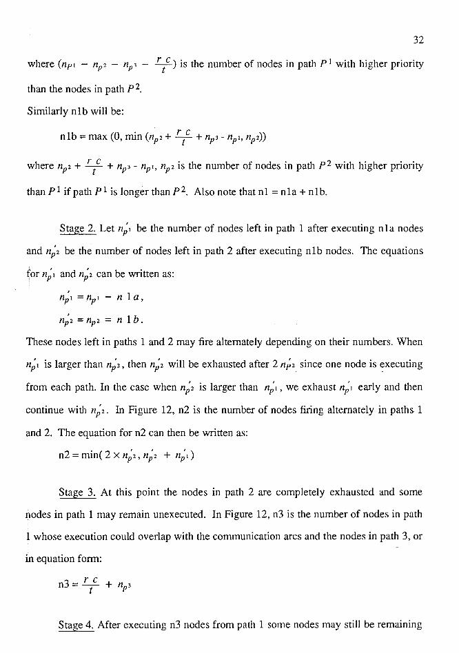
4.3.1 Global schedule

Figure 12 shows the general execution sequence of the graph when scheduled

globally. Let us analyse each stage of execution.

Stage 1. Depending on the length of paths 1, 2 and 3 some of the nodes in path 1

or path 2 may execute alone or may execute alternately. Let nl be the number of nodes

of either path 1 or path 2 that execute alone with no overlap. If nla and nlb are the

number of nodes of path 1 and path 2 respectively which execute alone, then nla will be:

nla = max(O, nµ1 - nµz - np3 - r /)

where (np1 - nµz - np3 - rt c) is the number of nodes in path P 1 with higher priority

than the nodes in path p2.

Similarly nlb will be:

32

where (np1 - nP2 - np3 - rt c) is the number of nodes in path P 1 with higher priority

than the nodes in path p2_

Similarly nlb will be:

nlb =max (0, min (np2 + r / + flp3 - np1, np2))

where np2 + r / + np3 - nP1, np2 is the number of nodes in path p2 with higher priority

than P 1 if path P 1 is longer than P 2. Also note that n 1 = n 1 a + n 1 b.

Stage 2. Let 11;1 be the number of nodes left in path 1 after executing nla nodes

and n;2 be the number of nodes left in path 2 after executing nlb nodes. The equations

(or n;1 and n;2 can be written as:

n; 1 = np 1 - n 1 a ,

n; 2 = nP 2 = n 1 b .

These nodes left in paths 1 and 2 may fire alternately depending on their numbers. When

n;1 is larger than 11;2, then n;2 will be exhausted after 2 n;z since one node is ~xecuting

from each path. In the case when n;2 is larger than n;1, we exhaust 11;1 early and then

continue with n;2. In Figure 12, n2 is the number of nodes firing alternately in paths 1

and 2. The equation for n2 can then be written as:

n2=min(2xn;2,n;2 + n;1)

Stage 3. At this point the nodes in path 2 are completely exhausted and some

nodes in path 1 may remain unexecuted. In Figure 12, n3 is the number of nodes in path I I 1 whose execution could overlap with the communication arcs and the nodes in path 3, or

in equation form:

r c n3 = -t- + 11p3

Stage 4. After executing n3 nodes from path 1 some nodes may still be remaining

12 is the number of nodes executed at stage 4, hence

n4 = n;;

4.3.2 Local schedule

Figure 13 shows the execution sequence when the graph is scheduled locally.

33

Stage 1. Since the local scheduler does not consider the communication time

when assigning weights to nodes of path 1 and path 2, more nodes in path 1 and path 2

will execute alone. nla and nl bin stage 1 of the local schedule case will be:

nla = max(O, nP1 - np2)

nlb = max(O, np2 - np1)

Stage 2. The number of nodes left in path 1 and path 2 after executing nla and

nlb nodes from path 1and2 will remain the same as those in global schedule.

n '1 = n 1 - n 1 a p p

n;2 = nP2 = n 1 b

n2 =min( 2 x n;2, n;2 + n;1)

Stage 3. The nodes left in path 1 can be overlapped by the communication

between processors and the nodes in path 3.

r c n3 = -t- + np3

Stage 4. The equations for nodes left in path 1 for execution after stage 3 will be

the same as in global schedule case.

" · ' n2 np 1 = nun ( np 1 - 2 - n 3, 0) = n4

Let us look at four examples in which we will try to predict the execution time of the

graph towards variation in lengths of paths 1, 2 and 3. The three examples are:

34

the same as in global schedule case.

,, · , n 2 np 1 = mm ( np 1 - T - n 3, 0) = n4

Let us look at four examples in which we will try to predict the execution time of the

graph towards variation in lengths of paths 1, 2 and 3. The three examples are:

1. Lengths of paths 1 and 2 are the same.

2. Length of path 1 is greater than path 2.

3. Length of path 2 is greater than path 1.

Lengths of paths 1 and 2 are the same

If we increase the lengths of path 1 and path 2, a linear increase in the difference

of execution time of global and locally scheduled graphs is expected to a certain point,

after which it should remain constant. The above statement is based on the following

interpretation:

1. Assuming that the communication time is greater than the execution time, i.e.,

c = z * t, the number of nodes in path 1 covered by the communication time

would depend on how big "z" is. In case of globally scheduled graphs, as we

increase the number of input nodes to path 1 and path 2, the number of overlap-

ping nodes in path 1 approaches a maximum value. The limit on the maximum

number of overlapping nodes in path 1 can be given by the foilowing simple

equation:

np3Xt + r xc maximum number of overlapping nodes = min ( np1, • )

where (np3 x t + r x c) is the time available for overlap and t is the execution

time of a node. Once crossed this number remains the same no matter how many

input nodes are added to path 1 and path 2.

2. On further increasing the number of input nodes to paths 1 and 2, the weights of

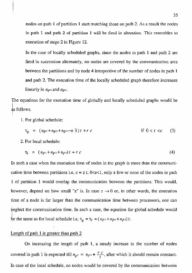
35

nodes on path 1 of partition 1 start matching those on path 2. As a result the nodes

in path 1 and path 2 of partition 1 will be fired in alteration. This resembles to

execution of stage 2 in Figure 12.

In the case of locally scheduled graphs, since the nodes in path 1 and path 2 are

fired in succession alternately, no nodes are covered by the communication arcs

between the partitions and by node 4 irrespective of the number of nodes in path 1

and path 2. The execution time of the locally scheduled graph therefore increases

linearly in npz and np1.

The equations for the execution time of globally and locally scheduled graphs would be

~s follows. !


'tg = (np1+np2+np3-n 3)t +r c if 0 < t <c (3)


tz = (np1+np2+np3)f+rc (4)

In such a case when the execution time of nodes in the graph is more than the communi-

cation time between partitions i.e, c = z t, O<z<l, only a few or none of the nodes in path

1 of partition 1 would overlap the communication between the partitions. This would,

however, depend on how small "z" is. In case z ~ 0 or, in other words, the execution

time of a node is far larger than the communication time between processors, one can

neglect the communication time. In such a case, the equation for global schedule would I be the same as for local schedule i.e, tg = t 1 = ( np1 + np2+ np3) t.

Length of path 1 is greater than path 2

On increasing the length of path 1, a steady increase in the number of nodes

covered in path 1 is expected till nµ 1 = np3 + rt c , after which it should remain constant.

In case of the local schedule, no nodes would be covered by the communication between

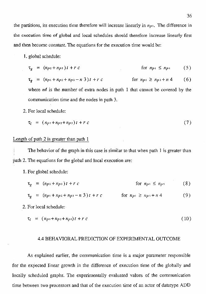
36

the partitions, its execution time therefore will increase linearly in np1. The difference in

the execution time of global and local schedules should therefore increase linearly first

kd then become constant. The equations for the execution time would be:

1. global schedule:

'tg (np2 + np3 ) t + r c for np1 ::;; np3 (5)

'tg = (np1 + np2 + np3 - n 3) t + r c for np1 ~ np3+n4 (6)

where n4 is the number of extra nodes in path I that cannot be covered by the

communication time and the nodes in path 3.


'tz = (np1+np2+np3)t +r c (7)

Length of path 2 is greater than path 1

I The behavior of the graph in this case is similar to that when path 1 is greater than I

path 2. The equations for the global and local execution are:


'tg = (np2 + np3 ) t + r c for np1 ::;; np3 (8)

'tg = (np1 + np2 + np3 - n 3) t + r c for np1 ~ np3+n4 (9)


t1 = (np1+np2+np3)t+rc (10)

4.4 BEHAVIORAL PREDICTION OF EXPERIMENT AL OUTCOME

I As explained earlier, the communication time is a major parameter responsible

I for the expected linear growth in the difference of execution time of the globally and

locally scheduled graphs. The experimentally evaluated values of the communication

time between two processors and that of the execution time of an actor of datatype ADD

37

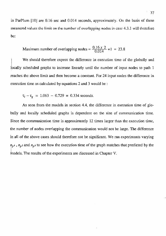
in ParPlum [10] are 0.16 sec and 0.014 seconds, approximately. On the basis of these

measured values the limit on the number of overlapping nodes in case 4.3.1 will therefore

be:

Maximumnumberofoverlappingnodes= 0}~!. 2 +1 = 23.8

I We should therefore expect the difference in execution time of the globally and i

iocally scheduled graphs to increase linearly until the number of input nodes to path 1

reaches the above limit and then become a constant. For 24 input nodes the difference in

execution time as calculated by equations 2 and 3 would be :

tz - tg = 1.063 - 0.729 = 0.334 seconds.

As seen from the models in section 4.4, the difference in execution time of glo

bally and locally scheduled graphs is dependent on the size of communication time.

Since the communication time is approximately 12 times larger than the execution time,

the number of nodes overlapping the communication would not be large. The difference

in all of the above cases should therefore not be significant. We ran experiments varying

np 1 , nP2 and np3 to see how the execution time of the graph matches that predicted by the I models. The results of the experiments are discussed in Chapter V.

CHAPTER V

EXPERIMENT AL RESULTS AND THEIR ANALYSIS

5.1 VARIATION IN PATHS 1AND2 (PATH 3 CONSTANT)

Tests were run on Parplum interpreter using a network of Sun workstations for

variations in the number of nodes ranging from 1 to 1200 for paths 1 and 2. The wall

clock time, which is also the total execution time in ParPlum, is the sum of the following

[10]:

1. Setup time: This is the time to create communication channels among all

processes.

2. Parser time: This is the time to parse the graph description and the machine

description.

3. Build link time: This is the time to build links between nodes in the graph.

4. Child execution time: This is the time taken by the child processes to execute -

parts of graph assigned to them.

The graphs were partitioned as shown in Figure 8 and the number of partitions

were always kept constant at 2. Table II shows the data gathered for total execution time

for ten test runs. The expected time as predicted by the models in Chapter IV is the child

Jxecution time. The expected time as shown in Table II is, however, a sum of the

expected setup time, parser time, build link time and the child execution time predicted

by our models. While gathering experimental data, the wall clock execution time and the

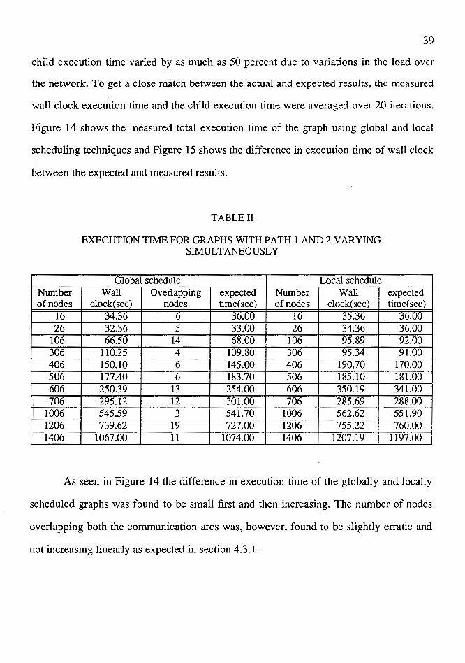
39

child execution time varied by as much as 50 percent due to variations in the load over

the network. To get a close match between the actual and expected results, the measured

wall clock execution time and the child execution time were averaged over 20 iterations.

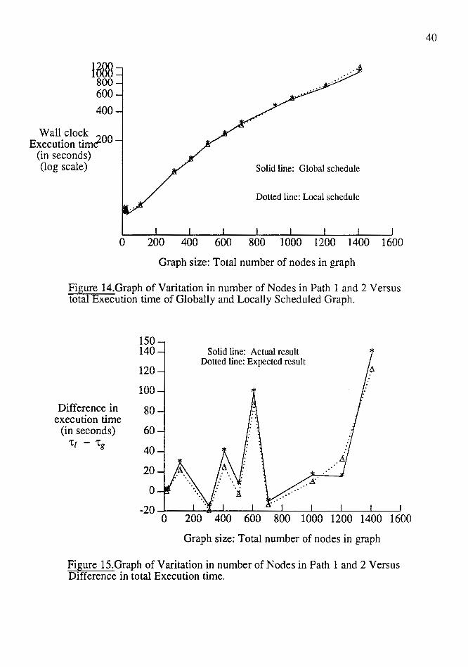
Figure 14 shows the measured total execution time of the graph using global and local

~cheduling techniques and Figure 15 shows the difference in execution time of wall clock

I lJetween the expected and measured results.

Number of nodes

16 26

106 306 406 506 606 706

I 1006 I

1206 1406

TABLE II

EXECUTION TIME FOR GRAPHS WITH PATH 1 AND 2 VARYING SIMULTANEOUSLY

Global schedule Local schedule Wall Overlapping expected Number Wall

clock( sec) nodes time( sec) of nodes clock( sec) 34.36 6 36.UU 16 35.36 32.36 5 33.00 26 34.36 66.50 14 68.00 106 95.89

110.25 4 109.80 306 95.34 150.10 6 145.00 406 190.70 177.40 6 183.70 506 185.10 250.39 13 254.00 606 350.19 295.12 12 301.00 706 285.69 545.59 3 541.70 1006 562.62 739.62 19 727.00 1206 755.22

1067.00 11 1074.00 1406 1207.19

expected time(sec)

36.uu 36.00 92.00 91.00

170.00 181.00 341.00 288.00 551.90 760.00

1197.00

As seen in Figure 14 the difference in execution time of the globally and locally

scheduled graphs was found to be small first and then increasing. The number of nodes

overlapping both the communication arcs was, however, found to be slightly erratic and

not increasing linearly as expected in section 4.3.1.

1088 800 600

400

Wall clock Execution timJOO

(in seconds) (log scale) Solid line: Global schedule

Dotted line: Local schedule

0 200 400 600 800 1000 1200 1400 1600

Graph size: Total number of nodes in graph

Figure 14.Graph of Varitation in number of Nodes in Path 1 and 2 Versus total Execution time of Globally and Locally Scheduled Graph.

150 140

120

100

Difference in 80 execution time

(in seconds) 60 't/ - 'tg

40

20

0

-20 0

Solid line: Actual result Dotted line: Expected result

200 400 600 800 1000 1200 1400 1600


Fi~ure 15.Graph of Varitation in number of Nodes in Path 1and2 Versus Difference in total Execution time.

40

t~ 14 12 10 8

Child 6 Execution time

(in seconds) 4 (log scale)

2 Solid line: Global schedule Dotted line: Local schedule

.A

0 200 400 600 800 1000 1200 1400 1600


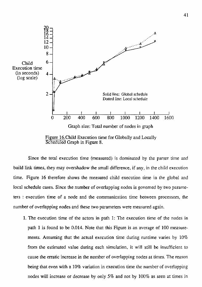
Figure 16.Child Execution time for Globally and Locally Scheduled Graph in Figure 8.

41

Since the total execution time (measured) is dominated by the parser time and

build link times, they may overshadow the small difference, if any, in the child execution

time. Figure 16 therefore shows the measured child execution time in the global and

local schedule cases. Since the number of overlapping nodes is governed by two parame-

ters : execution time of a node and the communication time between processors, the

number of overlapping nodes and these two parameters were measured again.

1. The execution time of the actors in path 1: The execution time of the nodes in

path 1 is found to be 0.014. Note that this Figure is an average of 100 measure

ments. Assuming that the actual execution time during runtime varies by 10%

from the estimated value during each simulation, it will still be insufficient to

cause the erratic increase in the number of overlapping nodes at times. The reason

being that even with a 10% variation in execution time the number of overlapping

nodes will increase or decrease by only 5% and not by 100% as seen at times in

42

nodes will increase or decrease by only 5% and not by 100% as seen at times in

Table II.

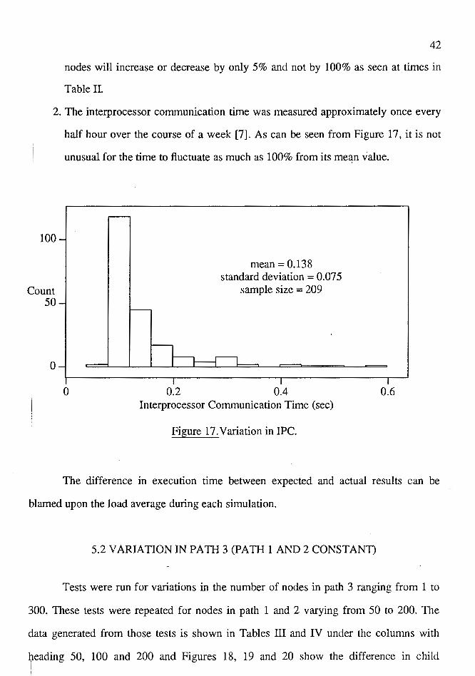
2. The interprocessor communication time was measured approximately once every

100

Count 50

0

half hour over the course of a week [7]. As can be seen from Figure 17, it is not

unusual for the time to fluctuate as much as 100% from its mean value.

0 0.2

mean= 0.138 standard deviation= 0.075

sample size = 209

0.4 Interprocessor Communication Time (sec)

Figure 17. V aria ti on in IPC.

0.6

The difference in execution time between expected and actual results can be

blamed upon the load average during each simulation.

5.2 VARIATION IN PA TH 3 (PATH 1 AND 2 CONST ANT)

Tests were run for variations in the number of nodes in path 3 ranging from 1 to

300. These tests were repeated for nodes in path 1 and 2 varying from 50 to 200. The

data generated from those tests is shown in Tables III and IV under the columns with

heading 50, 100 and 200 and Figures 18, 19 and 20 show the difference in child !

43

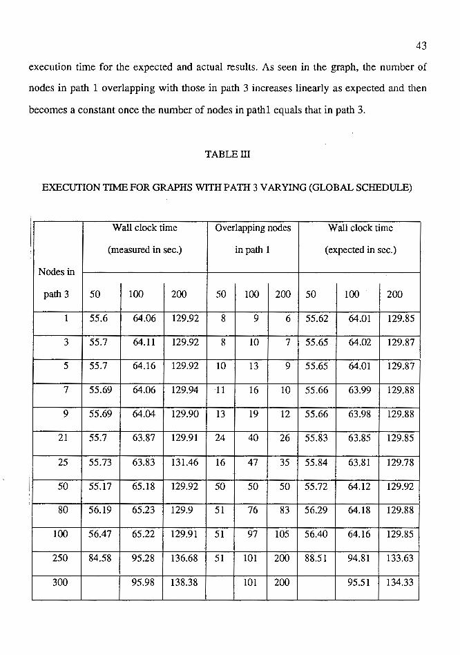
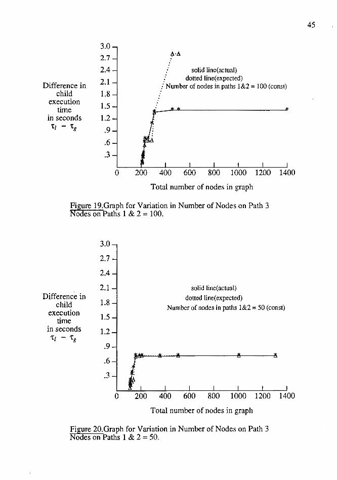
execution time for the expected and actual results. As seen in the graph, the number of

nodes in path 1 overlapping with those in path 3 increases linearly as expected and then

becomes a constant once the number of nodes in pathl equals that in path 3.

TABLE III

EXECUTION TIME FOR GRAPHS WITH PATH 3 VARYING (GLOBAL SCHEDULE)

Wall clock time Overlapping nodes Wall clock time

(measured in sec.) in path 1 (expected in sec.)

Nodes in

path 3 50 100 200 50 100 200 50 100 200

1 55.6 64.06 129.92 8 9 6 55.62 64.01 129.85

3 55.7 64.11 129.92 8 10 7 55.65 64.02 129.87

5 55.7 64.16 129.92 10 13 9 55.65 64.01 129.87

7 55.69 64.06 129.94 11 16 10 55.66 63.99 129.88

9 55.69 64.04 129.90 13 19 12 55.66 63.98 129.88

21 55.7 63.87 129.91 24 40 26 55.83 63.85 129.85

25 55.73 63.83 131.46 16 47 35 55.84 63.81 129.78

50 55.17 65.18 129.92 50 50 50 55.72 64.12 129.92

80 56.19 65.23 129.9 51 76 83 56.29 64.18 129.88

100 56.47 65.22 129.91 51 97 105 56.40 64.16 129.85

250 84.58 95.28 136.68 51 101 200 88.51 94.81 133.63

300 95.98 138.38 101 200 95.51 134.33

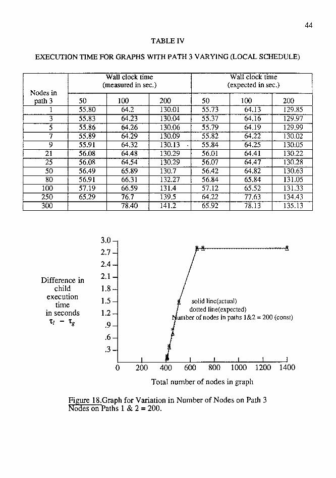
TABLE IV

EXECUTION TIME FOR GRAPHS WITH PATH 3 VARYING (LOCAL SCHEDULE)

Nodes in path 3 50

1 55.80 3 55.83 5 55.86 7 55.89 9 55.91

21 56.08 25 56.08 50 56.49 80 56.91

100 57.19 250 65.29 300

Difference in child

execution time

in seconds 'tz - 'tg

Wall clock time (measured in sec.)

100 64.2 64.23 64.26 64.29 64.32 64.48 64.54 65.89 66.31 66.59 76.7 78.40

3.0

2.7

2.4

2.1

1.8

1.5

1.2

.9

.6

.3

200 130.01 130.04 130.06 130.09 130.13 130.29 130.29 130.7 132.27 131.4 139.5 141.2

Wall clock time (expected in sec.)

50 100 55.73 64.13 55.37 64.16 55.79 64.19 55.82 64.22 55.84 64.25 56.01 64.41 56.07 64.47 56.42 64.82 56.84 65.84 57.12 65.52 64.22 77.63 65.92 78.13

solid line(actual) dotted line( expected)

200 129.85 129.97 129.99 130.02 130.05 130.22 130.28 130.63 131.05 131.33 134.43 135.13

umber of nodes in paths 1&2 = 200 (cons!)

0 200 400 600 800 1000 1200 1400

Total number of nodes in graph

Figure 18.Graph for Variation in Number of Nodes on Path 3 Nodes on Paths 1 & 2 = 200.

44

Difference in child

execution time

in seconds 't1 - 'tg

3.0

2.7

2.4

2.1

1.8

1.5

1.2

.9

.6

.3

~·A

solid line(actual) dotted line(expected)

.: Number of nodes in paths 1&2 = 100 (cons!)

0 200 400 600 800 1000 1200 1400



3.0

2.7

2.4

2.1 Difference in

child 1.8 execution 1.5 time in seconds 1.2 't[ - 'tg

.9

.6J

.3 -l

0 r

200

solid line(actual)

dotted line( expected)

Number of nodes in paths 1&2 = 50 (const)

A A A A

400 600 800 1000 1200 1400



45

46

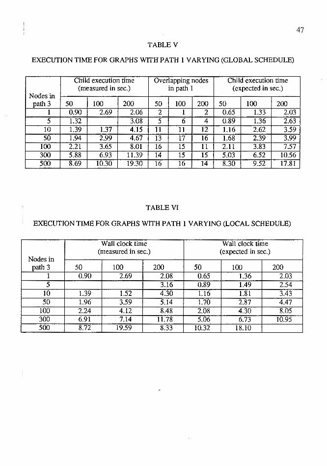
5.3 VARIATION IN PA TH 1 (PA TH 2 AND 3 CONST ANT)

Tests were run for nodes in the path 1 ranging from 1 to 1000. These tests were

repeated for nodes in path 2 varying from 50 to 200 while keeping nodes in path 3 con

stant to 10. The data generated for them is shown in the Tables V and VI under the

columns with headings 50, 100 and 200. Figures 21, 22 and 23 show the difference in

actual and expected child execution times for the globally and locally scheduled graph.

ts per equations 4 and 5 of section 4.3.3 one would expect that as the number of nodes

i'n path 1 are increased, the number of overlapping nodes in pathl with that in path 3

would increase linearly and then become a constant. Though this is reflected in the exper

imental results shown in Tables V and VI, the difference in execution time does not

become a constant once the number of overlapping nodes are constant. The execution

time as seen in Figures 21, 22 and 23 varies with variation in the number of nodes in path

2. The reason for such a behavior, is that, as the number of nodes in path 1 increases

they are assigned higher and higher priority than those in path 2. This results in some of

the nodes in path 1 firing alternately with the nodes in path 2. Since this sequence of

firing of nodes is similar to that usually observed in the local schedule case, the execution

time of the global schedule slowly starts approaching that of local schedule and the

9-ifference between them decreases. i

47

TABLE V


Child execution time Overlapping nodes Child execution time (measured in sec.) in path 1 (expected in sec.)

Nodes in path 3 50 100 200 50 100 200 50 100 200

1 0.90 2.69 2.06 2 1 2 0.65 1.33 2.03 5 1.32 3.08 5 6 4 0.89 1.36 2.63

10 1.39 1.37 4.15 11 11 12 1.16 2.62 3.59 50 1.94 2.99 4.67 13 17 16 1.68 2.39 3.99

100 2.21 3.65 8.01 16 15 11 2.11 3.83 7.57 300 5.88 6.93 11.39 14 15 15 5.03 6.52 10.56 500 8.69 10.30 19.30 16 16 14 8.30 9.52 17.81

TABLE VI


Wall clock time Wall clock time (measured in sec.) (expected in sec.)

Nodes in path 3 50 100 200 50 100 200

1 0.90 2.69 2.08 0.65 1.36 2.03 5 3.16 0.89 1.49 2.54

10 1.39 1.52 4.30 1.16 1.81 3.43 50 1.96 3.59 5.14 1.70 2.87 4.47

100 2.24 4.12 8.48 2.08 4.30 8.05 300 6.91 7.14 11.78 5.06 6.73 10.95 500 8.72 19.59 8.33 10.32 18.10

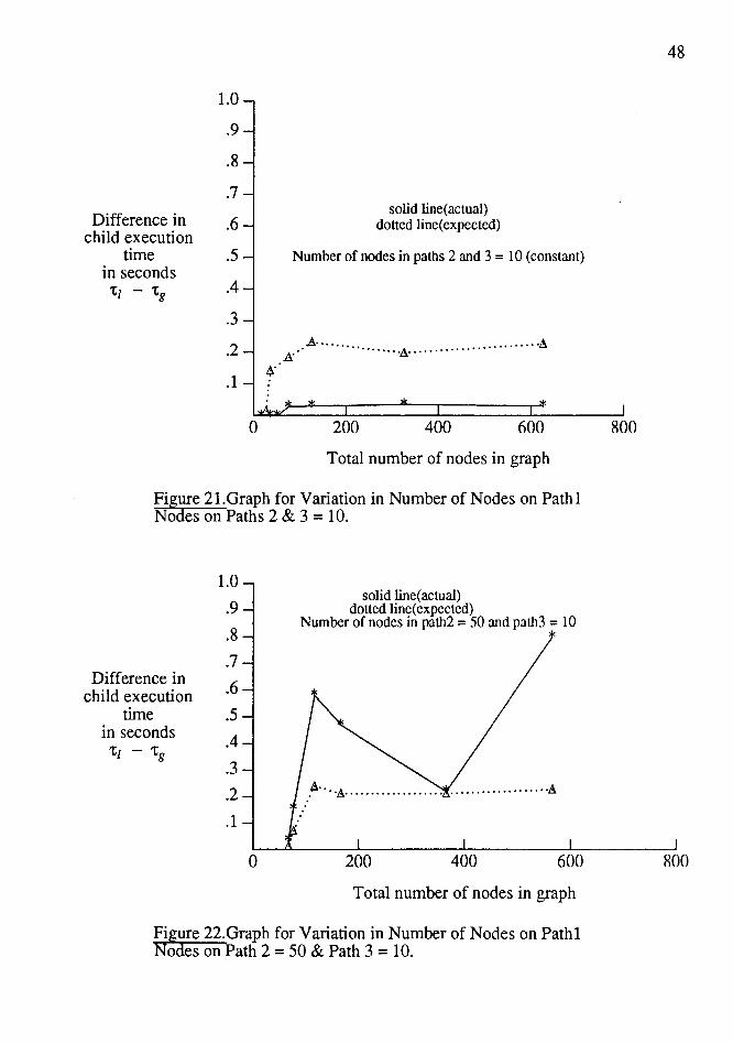
1.0

.9

.8

.7 Difference in .6

child execution time .5

in seconds tz - tg .4

.3

.2

.1 ~-

l 0


Number of nodes in paths 2 and 3 = 10 (constant)

A:· .A·················A·········· ···············A

200 400 600


Figure 21.Graph for Variation in Number of Nodes on Pathl Nodes on Paths 2 & 3 = 10.

1.0

.9

.8

.7 Difference in .6 child execution

time .5 in seconds

.4 tz - tg

.3

.2

.1 l 0


Number of nodes in path2 = 50 and path3 = 10

.~····A················-~··················A

200 400 600


Figure 22.Graph for Variation in Number of Nodes on Pathl Nodes on Path 2 = 50 & Path 3 = 10.

48

800

800

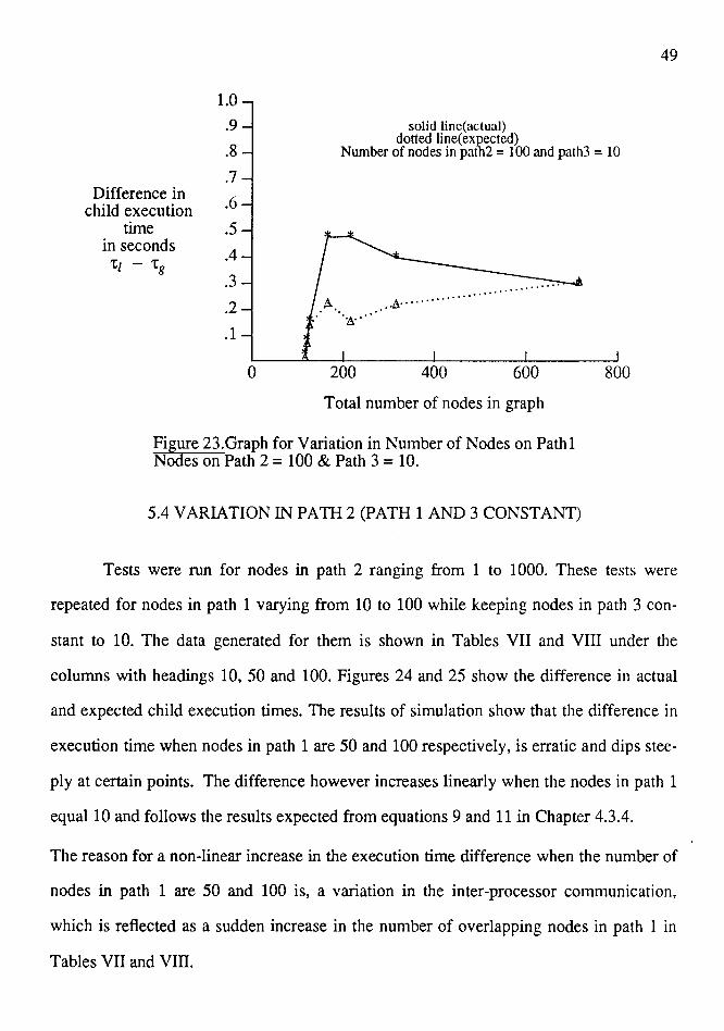
1.0

.9 solid line(actual) dotted line(expected)

.8 Number of nodes in patb2 = I 00 and path3 = 10

.7 Difference in .6 child execution

time .5 in seconds

.4 't/ - 'tg

.3

.2

.1 l 0 200 400 600


Figure 23.Graph for Variation in Number of Nodes on Pathl Nodes on Path 2 = 100 & Path 3 = 10.

5.4 VARIATION IN PATH 2 (PATH 1AND3 CONSTANT)

800

49

Tests were run for nodes in path 2 ranging from 1 to 1000. These tests were

repeated for nodes in path 1 varying from 10 to 100 while keeping nodes in path 3 con

stant to 10. The data generated for them is shown in Tables VII and VIII under the

columns with headings 10, 50 and 100. Figures 24 and 25 show the difference in actual

and expected child execution times. The results of simulation show that the difference in

execution time when nodes in path 1 are 50 and 100 respectively, is erratic and dips stee-

ply at certain points. The difference however increases linearly when the nodes in path 1

equal 10 and follows the results expected from equations 9 and 11 in Chapter 4.3.4.

The reason for a non-linear increase in the execution time difference when the number of

nodes in path 1 are 50 and 100 is, a variation in the inter-processor communication,

which is reflected as a sudden increase in the number of overlapping nodes in path I in

Tables VII and VIII.

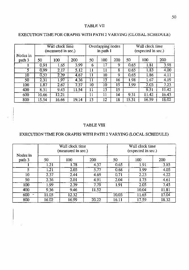
50

TABLE VII


Wall clock time Overlapping nodes Wall clock time (measured in sec.) in path 1 (expected in sec.)

Nodes in path3 50 100 200 50 100 200 50 100 200

1 0.91 1.65 3.99 6 17 9 0.65 1.81 3.98 5 0.99 2.17 5.12 11 11 8 0.65 1.83 4.00

10 0.57 2.39 4.67 11 10 9 0.65 1.86 4.11 50 2.31 1.97 4.36 11 13 16 1.98 1.67 4.19

100 1.87 2.67 7.37 10 10 15 1.99 2.03 7.23 400 8.31 9.43 11.54 11 13 15 9.51 11.42 600 10.66 12.21 11 11 14 9.31 11.42 16.43 800 15.54 16.66 19.14 13 12 18 15.31 16.59 18.02

TABLE VIII


Wall clock time Wall clock time (measured in sec.) (expected in sec.)

Nodes in path 3 50 100 200 50 100 200

1 1.21 1.78 4.37 0.65 1.91 3.85 5 1.21 2.03 5.77 0.68 1.99 4.03

10 2.37 2.44 4.69 0.71 2.23 4.22 50 2.36 2.01 4.91 2.04 1.75 4.61

100 1.99 2.39 7.79 1.91 2.05 7.45 400 9.36 9.46 11.52 10.04 11.81 600 - 11.05 12.32 10.03 11.65 17.04 800 16.02 16.99 20.22 16.11 17.59 18.32

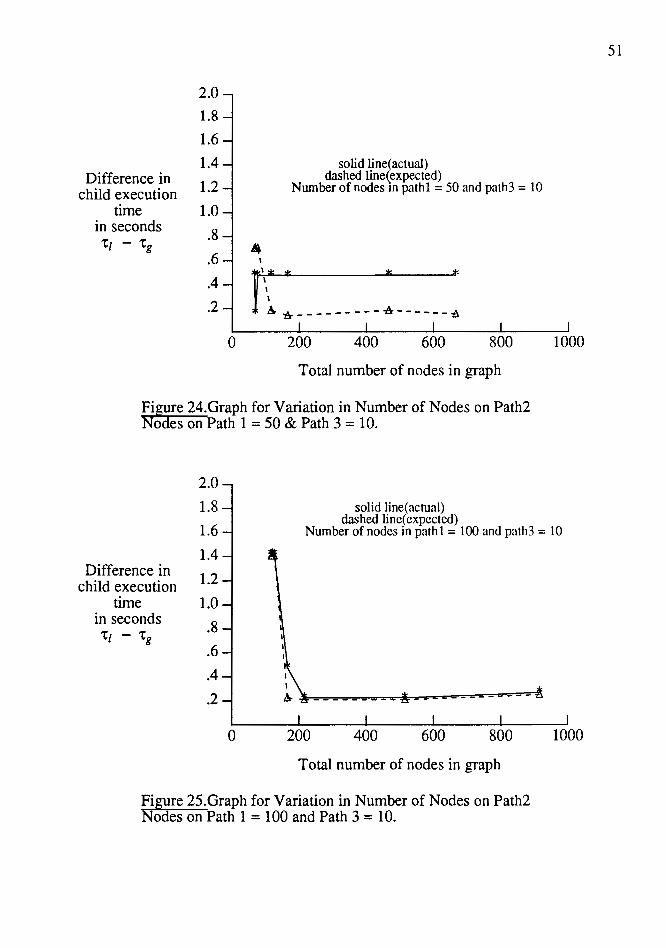
2.0

1.8

1.6

1.4 Difference in 1.2 child execution

time 1.0 in seconds .8 't[ - 'tg

. 6

.4

.2 l 0

.. I

solid line(actual) dashed line(expected)

Number of nodes m pathl = 50 and path3 = 10

r. . . "~,. _ - - --- - - _.,. ______ ..

200 400 600 800


Figure 24.Graph for Variation in Number of Nodes on Path2 Nodes on Path 1=50 & Path 3 = 10.

2.0

1.8

1000

1.6

solid line(actual) dashed line( expected)

Number of nodes in pathl = 100 and path3 = 10

1.4 Difference in 1.2 child execution

time 1.0 in seconds .8 't[ - 'tg

.6

.4

.2 l 0 200 400 600 800


Figure 25.Graph for Variation in Number of Nodes on Path2 Nodes on Path 1=100 and Path 3 = 10.

1000

51

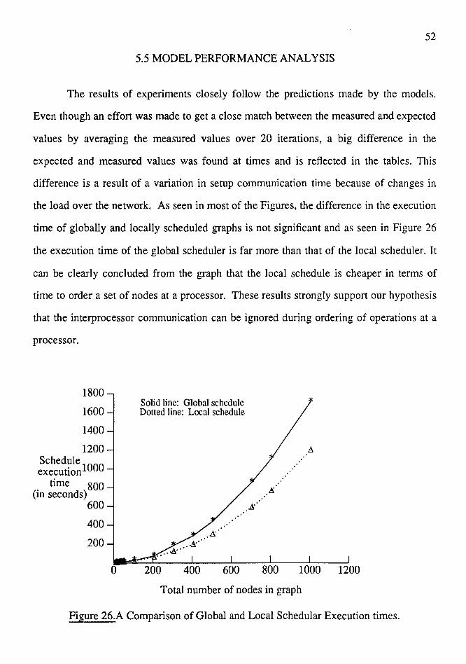
52

5.5 MODEL PERFORMANCE ANALYSIS

The results of experiments closely follow the predictions made by the models.

Even though an effort was made to get a close match between the measured and expected

values by averaging the measured values over 20 iterations, a big difference in the

expected and measured values was found at times and is reflected in the tables. This

difference is a result of a variation in setup communication time because of changes in

the load over the network. As seen in most of the Figures, the difference in the execution

time of globally and locally scheduled graphs is not significant and as seen in Figure 26

the execution time of the global scheduler is far more than that of the local scheduler. It

can be clearly concluded from the graph that the local schedule is cheaper in terms of

time to order a set of nodes at a processor. These results strongly support our hypothesis

that the interprocessor communication can be ignored during ordering of operations at a

processor.

1800 Solid line: Global schedule

1600 ~ Dotted line: Local schedule

1400

1200 Schedule execution 1000

time 800 (in seconds)

600

400

200

0 200 400 600

A

.· .· •• .e;."

~

800 1000 1200


Figure 26.A Comparison of Global and Local Schedular Execution times.

CHAPTER VI

CONCLUSION

6.1 SIGNIFICANCE OF THIS RESEARCH

This thesis presented an analysis of ignoring inter-processor communication dur-

ing intraprocessor scheduling. Scheduling in our sense is different than that suggested in

most of the literature available in that it does not include allocation. To aid this research

two scheduling techniques, namely, global and local, have been suggested in Chapter II. I

Intraprocessor scheduling is important because it can take advantage of parallelism I

among nodes in a given task at a processor, and order the execution sequence of those

nodes at the processor. This ordering can result in a reduced execution time of the sub-

graph, depending on the efficiency of the scheduling algorithm used. Eight scheduling

heuristics have been implemented in the ParPlum system. However, Granski's schedul

ing algorithm is the most effective among them and has been used for evaluating the glo

bal and local scheduling techniques. To test the techniques a graph was sought after,

which identified some properties that are necessary to see a difference in global and local

schedules. For fork and join graphs, the key property is: A path in a program has to be cut

and its pieces assigned to different processors to see a difference in relative priorities.

An analysis of the results suggests that the difference between globally and

locally scheduled graphs is visible only when a graph depicts the property mentioned

above and when communication time is larger than the execution time of a node. In other

cases the models and experimental results show no difference in the execution time of

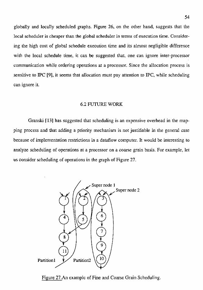
54

globally and locally scheduled graphs. Figure 26, on the other hand, suggests that the

local scheduler is cheaper than the global scheduler in terms of execution time. Consider-

ing the high cost of global schedule execution time and its almost negligible difference

with the local schedule time, it can be suggested that, one can ignore inter-processor

communication while ordering operations at a processor. Since the allocation process is

sensitive to IPC [9], it seems that allocation must pay attention to IPC, while scheduling

can ignore it.

6.2 FUTURE WORK

Granski [ 13] has suggested that scheduling is an expensive overhead in the map-

ping process and that adding a priority mechanism is not justifiable in the general case

because of implementation restrictions in a dataflow computer. It would be interesting to

analyze scheduling of operations at a processor on a coarse grain basis. For example, let

us consider scheduling of operations in the graph of Figure 27.

/ Super node 1 /Super node 2

Partition! ~ Partition2

Figure 27 .An example of Fine and Coarse Grain Scheduling.

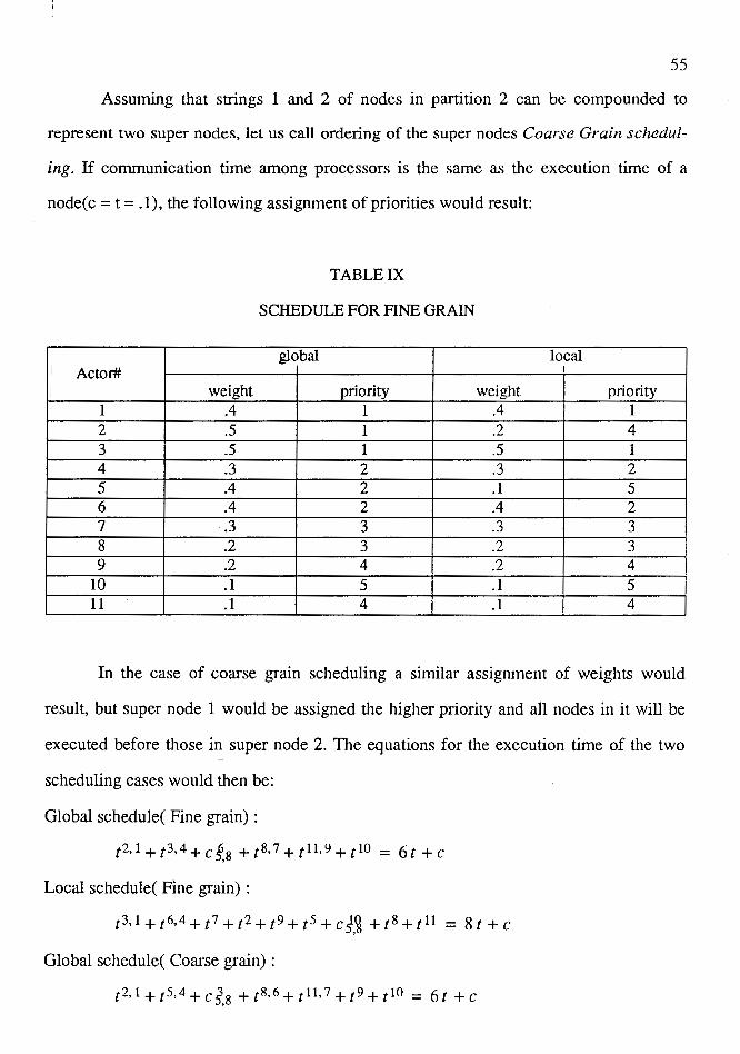
55

Assuming that strings 1 and 2 of nodes in partition 2 can be compounded to

represent two super nodes, let us call ordering of the super nodes Coarse Grain schedul-

ing. If communication time among processors is the same as the execution time of a

node(c = t = .1), the following assignment of priorities would result:

TABLE IX

SCHEDULE FOR FINE GRAIN

i global local

I Actor# i weight priority weight priority

1 .4 1 .4 1 2 .5 1 .2 4 3 .5 1 .5 1 4 .3 2 .3 2 5 .4 2 .1 5 6 .4 2 .4 2 7 -.3 3 .3 3 8 .2 3 .2 3 9 .2 4 .2 4

10 .1 5 .1 5 11 .1 4 .1 4

In the case of coarse grain scheduling a similar assignment of weights would

result, but super node 1 would be assigned the higher priority and all nodes in it will be

~xecuted before those in super node 2. The equations for the execution time of the two ! scheduling cases would then be:

Global schedule( Fine grain) :

t2,l+t3,4+cfg +t8,7+tll,9+t10 = 6t +c ,

Local schedule( Fme grain) :

t3,l+t6,4+t7+t2+t9+t5+c5:~+t8+tll = St+c ,

Global schedule( Coarse grain) :

t2,l+t5,4+c~,8 +t8,6+tll,7 +t9+tl0 = 6t +c

56

Local schedule( Coarse grain) : I

t3,l+t6,4+t1+t9+t1D+t2+t5+c 5.8+t8+tll = 9t +c

The equation for the coarse grain local schedule shows a smaller difference in execution

time than those in the fine grain case. Since a coarse grain schedule would take shorter

time to produce than a fine grain schedule, one would obviously choose the former while

sacrificing the small difference in execution time. This is an interesting property and

could be studied further.

All analysis in this thesis assumed that a processor could have only one ALU. If,

however, the number of ALU's available in each processor grows to more than the

number of ready operations at that processor, then there would be no need to schedule the

operations. On the contrary, if the number of available ALU's is less than the operations,

c!me feels a strict need of scheduling. The performance of parallel execution is therefore a ! I

function of the number of available ALU's. This is an interesting topic and can be stu-

died further.

All of the graphs tested for this thesis had nodes of the same datatype. This

notion, though convenient for our testing, is not mandatory and graphs having nodes of

different data types should be executed for global and local schedules. For our experi-

mental purpose we chose a very simple graph. However, more complex graphs should be

tested. Two models have been extensively used in estimating the execution time of a

node and the communication time between processors in Gran ski's algorithm and also in

the equations for global and local schedules shown in Chapter IV. The behavior of global

and local schedules towards inaccuracies in those models would be worth looking into.

To avoid the variations in the parameters because of changes in the load average on the

system, the simulator could be implemented on a dedicated multiprocessor, such as

Intel's Hypercube.

57

REFERENCES

[1] Adam, T. L., K. M. Chandy, and J. R. Dickson, "A Comparison of List Schedules for Parallel Processing Systems," Communications ACM , vol. 17, no. 12, pp. 685-690, December 12, 1974.

[2] Anger, F. D., J. Hwang, and Y. Chow, "Scheduling with Sufficiently Loosely Coupled Processors," Journal of Parallel and Distributed Computing, vol. 9, pp. 87-92, 1990.

[3] Appelbe, W. F. and M. R. Ito, "Scheduling Heuristics in a Multiprogramming Environment," IEEE Transactions on Computers, vol. c-27, no. 7, pp. 628-637, July 1978.

[4] Coffman, E. G., "Computer and Job-Shop Scheduling Theory," John Wiley & Sons, New York, 1976.

[5] Driscoll, M.A., P. R. Prins, P. D. Fisher, and L. M. Ni, "Efficient Scheduling of Datafiow Graphs for Multiprocessor Architectures," Rep. no. MSU-ENGR-88-008, College of Engineering, Michigan State University June, 1988.

[6] Driscoll, M.A. and P. D. Fisher, "On Partitioning of Algorithms for Parallel Execution on VLSI Circuit Architectures," Rep. no. MSU-ENGR-88-016, College of Engineering, Michigan State University, September, 1988.

[7] Driscoll, M.A., J. Fu, S. M. Pai, C. Patwardhan, L. Setiowijoso, D. Tang, and K. Thayib, "Sensitivity Analysis and Mapping Programs to Parallel Architectures," Presented at the 1991 International Conference on Parallel Processing , August 1991.

[8] Efe, K., "Heuristic Models of Task Assignment Scheduling in Distributed Systems," Computer, vol. 15, pp. 50-56, June 1982.

[9] El-Rewini, H. and T. G. Lewis, "Scheduling Parallel Program Tasks onto Arbitrary Target Machines," Journal of Parallel and Distributed Computing , vol. 9, pp. 138-158, 1990.

[10] Fu, J., "PARPLUM A System for Evaluating Parallel Program Optimization Methods," M.S Thesis, Department of Electrical Engineering, Portland State University, 1991.

58

[11] Gonzalez, M. J. Jr., "Detenninistic Processor Scheduling," Computing Surveys , vol. 9, no. 3, pp. 173-204, September 1977.

[12] Graham, R. L., "Bounds on Multiprocessor Timing Anomalies," SIAM J. Appl. Math. , vol. 17, pp. 416-429, 1969.

[13] Granski, M., "The Effect of Operation Scheduling on the Performance of a Data Flow Computer," IEEE Transaction on Computers, vol. C-36 no. 9, September 1987.

[14] Ha, S. and E. A. Lee, "Compile Time Scheduling and Assignment of Data-FLow Graphs with Data-Dependent Iteration," IEEE Transaction on Computers , vol. 40, no. 11, Nov. 1991.

[15] Hu, T. C., "Parallel Sequencing and Assembly Line Problems," Oper. Res. , vol. 9, 841-848, November 1961.

[16] Hwang, J., Y. Chow, F. D. Anger, and C. Lee, "Scheduling Precedence graphs in Systems with Interprocessor Communication Times," Siam J. Computing , vol. 18, no. 2, pp. 244-257, April 1989.

[17] Jordan, H., "The Characteristics of Parallel Algorithms," Chapter 16 MIT Press, Cambridge, MA, 1987.

[18] Karp, A., "Programming for Parallelism," Computer , vol. 15, pp. 43-57, May 1987.

[19] Kasahara, H. and S. Narita, "Practical Multiprocesor Scheduling Algorithm for Efficient Parallel Processing," IEEE Transactions on Computer, vol. c-33, no. 11, pp. 1023-1029, November 1984.

[20] Kaufman, M. T., "An Almost-Optimal Algorithm For The Assembly Line Scheduling Problem," IEEE Transactions on Computers, vol. C-23, 1169-1174, Nov. 1974.

[21] Kohler, W. H., "A Preliminary Evaluation of the Critical Path Method for Scheduling Tasks on Multiprocessor Systems," IEEE Transactions on Computers , vol. c-15, no. 12, pp. 1235-1238, December 1975.

[22] Kruatrachue, B., "Static Task Scheduling and Grain Packing in Parallel Processing Systems," Ph.D Thesis, Department of Computer Science, Oregon State University, 1987.

[23] Kunde, M., "Nonpreemptive LP-Scheduling on Homogeneous Multiprocessor Systems," SIAM J. Computing, vol. 10, no. 1, pp. 151-173, Feb. 1981.

59

[24] Lenstra, J. K. and A.H. G. Rinnooy Kan, "Complexity Of Scheduling Under Precedence Constraints," Operations Research , vol. 26, no. 1, pp. 22-35, Jan.-Feb. 1978.

[25] Li, Hon F., "Scheduling Trees in Parallel/Pipelined Processing Environments," IEEE Transactions on Computers , vol. c-26, no. 11, pp. 1101-1112, November 1977.

[26] Martin, D. and G. Estrin, "Models of Computation and System Cyclic to Acyclic Graph Transformations," IEEE Transaction Elec. Comput. , vol. C-16, pp. 70-79, Feb. 1967.

[27] Papadimitriou, C. H. and J. D. Ullman, "A Communication-Time Tradeoff," SIAM J. Comput. , vol. 6, no. 4, pp. 639-646, Aug. 1987.

[28] Polychronopoulos, C. D. and D. J. Kuck, "Guided Self-Scheduling: A Practical Scheduling Scheme for Parallel Supercomputers," IEEE Transaction on Computers, vol. C-36, no. 12, pp. 1425-1439, December 1987.

[29] Ramamoorthy, C., K. M. Chandy and M. J. Gonzales, "Optimal Scheduling Strategies in a Multiprocessor System," IEEE Transaction Computer, vol. C-21, pp. 37-146, Feb. 1972.

[30] Ramamoorthy, C. and W. H. Leung, "A Scheme for Parallel Execution of Sequential Programs," Proc. of 1976 International conference on Parallel Processing, pp. 312-316, 1976.

[31] Rayward-Smith, V. J., UET "Scheduling with Interprocessor Communication Delays," Internal Report SYS-C86-06, School of Information Systems, University of East Anglia, Norwich, United Kingdom, 1986

[32] Sarkar, V., "Partitioning and Scheduling Parallel Programs for Multiprocessors," The MIT Press, 1989.

[33] Sethi, R. and Ravi, "Scheduling Graphs on Two Processors," SIAM J. Comput, vol. 5, no. 1, pp. 73-82, March 1976.

[34] Simmons, M., R. Koskela, and I. Bucher, "Instrumentation for Future Parallel Computing Systems," Addison Wesley Publishing Company , 1989. -

Documents

Ignoring Interprocessor Communication During Scheduling