29 – 30 January 2010 CESifo Conference Centre, Munich

A joint initiative of Ludwig-Maximilians University’s Center for Economic Studies and the Ifo Institute for Economic Research

Temporary Workers and Seasoned Managers as Causes of Low Productivity

Francesco Daveri and Maria Laura Parisi

CESifo GmbH Phone: +49 (0) 89 9224-1410 Poschingerstr. 5 Fax: +49 (0) 89 9224-1409 81679 Munich E-mail: office@cesifo.de Germany Web: www.cesifo.de

Ifo / CESifo & OECD Conference on Regulation:

PPoolliittiiccaall EEccoonnoommyy,, MMeeaassuurreemmeenntt aanndd EEffffeeccttss oonn PPeerrffoorrmmaannccee

This draft: January 15, 2010

Temporary workers and seasoned managers as causes of low productivity

Francesco Daveri Maria Laura Parisi

Università di Parma, Università di Brescia Igier and CESifo

Abstract

We employ company micro data to study the determinants of low productivity growth in the Italian economy. We show that the acute productivity slowdown witnessed in the last few years has manifested itself in parallel with two factors seemingly stifling innovation: the presence of a high share of temporary workers and the old age and high seniority of top managers and members of the boards. These results may be seen as providing elements consistent with both a “labor supply view” and a “labor demand view” of Italy’s productivity slowdown.

An earlier draft of this paper was presented in Aix-en-Provence. We are grateful to Gilbert Cette and our discussant Remy Lecat for their useful comments.

1. Introduction After decades of fast growth that led Italian living standards to converge towards European levels by the end of the 1980s, GDP growth in Italy has markedly slowed down since the mid 1990s. Figure 1 below shows that, since 1995, Italy’s GDP has cumulatively lost some twenty percentage points vis-à-vis the GDP of the other four big countries in the European Union (Germany, France, the UK and Spain). Hence Italy’s prolonged growth slowdown has been a mystery to explain long before the Great Recession of 2008 and 2009.

Figure 1. - GDP growth in Italy and in the other big four European countries, 1995-2008

Source: Francesco Daveri, “Italy, before and after Lehman Brothers”, VoxEu.org, June 5, 2009

Italy’s declining growth performance – the continuation of a secular trend only partially shared with other OECD countries - has been the combination of two distinct – though as we will discuss possibly interrelated - labor market developments. There has been a marked decline - from 2.1% in 1980-95 to 0.5% after 1995 - in the growth rate of labor productivity. Yet this productivity slowdown has been paralleled by a marked increase in the growth rate of total hours worked, which turned from negative to positive figures. Both developments have been quite at odds with what had happened in previous decades. Table 1 - Decomposing Italy’s per-capita GDP growth, 1970-2004

Growth rates of Per-capita GDP GDP per

hour worked Hours per working age person

Working age population over total population

1970-80 3.1 3.9 -0.8 0.0

1980-95 1.8 2.1 -0.7 0.4

1995-04 1.3 0.5 1.0 -0.2

Source: Daveri and Jona Lasinio (2005)

As shown in Table 2, productivity started its stagnation after 1995 in both manufacturing and

service industries. Yet, while the presence of stagnating or even declining productivity is not surprising in the services industries, especially in a country like Italy whose services are still plagued with extensive monopolistic provision, the particularly striking features of these developments has been the zeroing of productivity growth in the Italian manufacturing industries. This is notable because manufacturing industries have been “the” productivity-leading industries in Italy in the past decades. This declining path has been particularly pronounced during the 2001-03 aggregate slowdown, when labor productivity growth has gone down below zero, but it was there even in 1995-00 when the economy was doing relatively well. Italy’s productivity slowdown is not the consequence of unfortunate business cycle fluctuations. Table 2 - Growth of labor productivity in Italy, 1970-2003, main industry groups

1970-80 1980-95 1995-03 1995-00 2000-03

Economy 2.4 1.8 0.6 1.1 -0.2

Agriculture 3.1 4.3 2.7 5.2 -1.5

Manufacturing 2.8 3.0 0.2 1.0 -1.0

-- non-durables 2.7 3.1 0.3 0.7 -0.2

-- durables 2.9 2.7 0.0 1.7 -2.7

Utilities -0.4 0.8 5.5 3.7 8.7

Construction 1.9 1.0 0.1 0.5 -0.5

Business sector services 1.8 1.1 0.1 0.5 -0.5

Public services 1.4 0.7 0.4 0.8 -0.1

Source: Daveri and Jona-Lasinio, 2005

In this paper, we take a look backwards to 2001-03, a period of particularly acute slowdown in the Italian economy and less so elsewhere in Europe, to learn about the possible determinants of productivity developments at the firm level. Our micro data evidence indicates that productivity growth was particularly low in firms with disproportionately high shares of temporary workers to start with. This result is robust to all changes of specifications. Yet declining productivity is also – slightly less robustly - associated to such managerial features as the average age and seniority of the managers running the companies. Our estimates separately run for innovative and non-innovative companies indicate that seniority do not seem to play a major role, while an older age of managers is associated with lower productivity in innovative firms and with higher productivity in non-innovative firms. This is consistent with common sense that suggests a more positive role of experience in firms with relatively standardized and stable business practices, while old age and seniority is presumably more damaging for innovative firms that would be supposed to swiftly adopt new technologies as they become available. This is presumably more tightly correlated with schooling and less with experience on the job. Our 2-stage model results, while confirming the robustness of the partial correlation between the share of temporary workers and productivity, shows that both product and process innovation are positively related with productivity growth. For the innovative firms age is negatively correlated with productivity growth and zero or positively correlated with non innovative firms, throughout all estimation methods used.

The relation between managerial seniority and productivity is instead less tightly correlated than within the OLS framework. The correlation between seniority and productivity varies considerably across specifications. It appears always non correlated for innovative firms, while the correlation is ambiguous for non innovative firms and depends on the estimation method being used. Our paper is structured as follows. In section 2, we present the two main competing explanations for Italy’s productivity slowdown in words. In section 3 we present the paper’s conceptual underpinnings and a theoretical model of managerial capital and productivity that nests the two hypotheses. In section 4 we illustrate our econometric framework. In section 5 and 6 we describe the main features of the data set and our estimation results. Section 7 concludes. 2. Italy’s productivity slowdown: two explanations

This sudden productivity turnaround witnessed in the Italian economy after the mid 1990s begs an explanation. A view shared by many Italian entrepreneurs is the so called “Labor Supply” view – consistent with the ideas expressed by Robert Gordon and Ian Dew-Becker (2008) on the interrelation between labor market reform and productivity developments in Europe. In their paper, they conjectured that the process of - mostly piecemeal - labor market reform that occurred in many European countries, while helping Europe reverse the past tendencies towards job destruction, has been eventually detrimental to productivity growth. Simplifying their view to an extreme, if labor market reform occurs and labor demand does not shift, labor supply shifts to the right along a given labor demand curve. No wonder that productivity declines as a result. This may have occurred in Italy as well, in the wake of the changes in labor market legislation in favor of more flexibility introduced by the Prodi Government in 1997-98. These legislative changes gave full legal recognition to a host of contractual forms of part-time and temporary jobs, some of which had been in place even before though restricted to the unofficial labor market. The flurry of cheap labor originated from such half hearted labor market reforms has resulted in a decline of the equilibrium capital-labor ratio. It may have also discouraged the innovative ability of many entrepreneurs who found themselves confronted with the hard-to-resist temptation to adopt techniques intensively using the part-time workers now abundantly available in the labor market. Yet the labor supply view is not the only game in town. Another potential explanation would stress the role of labor demand, and notably of the interplay between a changing world economy and a largely unchanged domestic managerial environment. The majority of Italian firms, typically agglomerated in industrial districts or involved as sub-contractors by large-scale exporting companies, simply continued their previous business conducts. Yet the mode and the opportunities of competition around the world had changed meanwhile. There was a technological revolution out there whose fruits could have been reaped by those companies adopting the new technologies as well as adapting their managerial techniques to the changed environment. Yet the Italian economy was not well equipped for withstanding competition in this changing world. In a recent paper, Bandiera, Guiso, Prat and Sadun (2008) have analyzed the incentive structure that Italian managers face, their career profile and even their use of time. It turns out that only a fraction of firms – especially the non-family owned and multinationals - adopts a “performance-based” model, whereby managers are hired through formal channels such as business contacts and head-hunting activities, undergo regular assessment procedures and are rewarded, promoted and dismissed on the basis of their assessment results. Most firms – particularly the family-owned ones and those mainly active in the domestic market - follow a “fidelity model” of

managerial talent, hiring their managers based on personal or family contacts, without formally assessing their performance and promoting and rewarding them according to the quality of their personal relations with the firm’s owners. The problem is that the type of managerial model – based on performance or fidelity – is tightly associated with the quality, the conduct and the performance of managers as well as of the firm itself. And here then comes our second explanation of Italy’s productivity slowdown: firms endowed with managers of such poor quality are presumably at a disadvantage when faced with new technological opportunities with respect to foreign competitors less dependent on family-based modes of running a firm. While there may be some grains of truth in both views, Gordon and Dew-Becker have not contrasted their ideas with micro data, while Bandiera, Guiso, Prat and Sadun have not looked at the interaction of labor market reform with the productivity and innovation counterpart of managerial practices. So there is room for comparing a streamlined version of the two views against the backdrop of the same data set. This is the main goal of our paper. If the Labor Supply view is correct, we expect to see in the data more pronounced productivity declines in companies with disproportionately higher shares of part-time and temporary workers at the beginning of the period. If the Labor Demand view is correct, we expect to detect stronger productivity declines in companies with older and/or senior managers. Ceteris paribus, older CEOs, board members and managers are possibly less prone to introduce new technologies and innovation, because this may change their routines and more importantly if this changes the circulation and transmission of information within the firm and eventually the structure of power within the firm. Yet age as such may not be the crucial or the only element to consider in this respect. As emphasized by Daveri and Maliranta (2007) for a large sample of Finnish manufacturing companies and workers, seniority may be the really damaging feature, particularly in high-tech companies where a certain attitude towards change is more likely related to short tenure and lack of entrenchment in a given company. Both explanations may have something to say on Italy’s productivity decline and perhaps more generally. We simply construct our thought experiment to let the data speak on this. 3. Managerial effort, business schooling and firm productivity Before delving into our empirical analysis, we make our working hypotheses more precise within a logically coherent two-period production function framework. The manager side A manager lives for two periods. Today she can either exert managerial effort (“work”) or go to school - a business school, where she learns novel managerial techniques to be employed at work tomorrow. Tomorrow she cannot but work for, in a two-period framework, there is no point to go a business school any more. If working (e>0) she earns a compensation v in each period. Hence her lifetime income equals 2v. This income finances lifetime consumption. With zero discount and interest rates and standard preferences, the working manager will smoothly consume ce*= v + ε/2 in each period. If instead she decides to go to the business school today, she postpones working to tomorrow and e=0. In the meanwhile, she learns new business techniques, so that she accumulates managerial

capital (b>0). Tomorrow, endowed with the new business techniques b, she will earn a compensation w>v. Then, the lifetime income of an educated manager is w. Again, with zero discount and interest rates (and perfect access to credit markets), consumption smoothing will prevail under standard preferences, so that cb*= w/2 in each period. 1

Note that the educated managers are ”young” in the labor market, for they have no work experience, while the uneducated managers are “old” (i.e. experienced but unaware of new business techniques). The firm side Firms are born all alike. Then R&D investment (or abundance of cash flow or other circumstances enhancing the chance that a firm becomes innovative) may materialize or not. If any of such circumstances takes place, the firm becomes an innovative firm (an I-firm). If R&D does not take place, the firm stays non-innovative and becomes an N-firm. The difference between the two types of firms stems from their production function. The production function of each N firm is as follows: YN = AN KN

αLNβ

where α>0, β>0, 0<α+β<1, KN

and LN are respectively the stock of capital and the number of workers employed in each firm N, AN is the scale parameter in the production. The parameter AN depends on past managerial effort as follows: AN =EN,-1

(1-α-β) with EN=ΣeN. In words, the efficient level of production in firm N is a function of capital, labor and managerial capital. In turn, managerial capital is accumulated through managerial effort under diminishing returns. With this production function, labor productivity yN= YN/LN is: (a) decreasing in LN and (b) increasing in EN,-1 The innovative firms are different from the non-innovative ones for the quality of managerial effort being required. They employ capital and labor as well as traditional and new managerial techniques. Traditional managerial techniques require experience, while new managerial techniques are those accumulated through business schooling. Efficient production occurs through the following production function: YI = AIKI

α LIβ

1 In the schooling case, access to credit market certainly makes a difference for the consumption path. If credit market constraints prevent or restrict borrowing to fund her schooling of today, c2* > c1*, i.e. the consumption path of the manager will be upward sloping. We do not study empirically the consumption path implication of the managerial decision.

where α>0, β>0, 0<α+β<1, KI and LI are respectively the stock of capital and the number of

workers employed in each firm I, while AI is the efficiency parameter in the production. AI is a function of past managerial effort and business schooling as follows: AI =EI,-1

(1-α-β) + B with EI=ΣeI and B=Σb, where B is managerial capital accumulated at the business school in the previous period by those who are employed as managers in I-firms. In words, the efficient level of production in firm I is a function of capital, labor and managerial capital. In turn, managerial capital is accumulated through managerial effort under diminishing returns and through business schooling under constant returns. This is different from the N-firms: for an I-firm, being endowed with a young With this production function, labor productivity yI= YI/LI is: (a) decreasing in LI and (b) increasing or decreasing in EI,-1, depending on whether the positive effect of work on AI more than offsets the negative effects from the foregone accumulation of business school capital entailed by the decision to work instead of going to the business school Equilibrium allocation of managers Each firm hires managers with the goal of maximizing its profits. For each firm N and I this entails equalization of marginal productivity of experienced managers to their compensation v. In turn, for firm I, profit maximization also entails equalization of the marginal productivity of experienced managers to the marginal productivity of educated managers, which has to be equal to w. The following list of equilibrium conditions follow: (1-α-β)EN,-1

(-α-β) KNαLN

β = v (1-α-β)EI,-1

(-α-β) KIαLI

β = v KI

αLIβ = w

M= iB + nEN,-1+ iEI,-1 The latter of which is a condition of full employment of managers, with M being the total number of managers, i the total number of I firms and n the total number of N firms. The four conditions above determine, up to a given level of K and L, the hiring of uneducated and educated managers in the two groups of firms and the business schooling premium w/v. Empirical implications Summing up, the model’s implications that we will exploit in the empirical part of our paper are the following:

(a) Firms select themselves into innovative and non-innovative ones depending on some exogenous circumstances such as the occurrence of R&D spending, the presence of enough cash flow and others to be specified.

(b) Experience is good for labor productivity in the non-innovative firms and either good or bad for productivity in the I-firms. We will use managerial seniority as a measure of managerial experience within the firm. Managerial age will be a measure of overall managerial experience over and above the experience gained within a given firm.

(c) Labor market liberalization and other measures that tend to favor the entry of unskilled workers is equally bad for labor productivity in both types of firms.

4. Econometric framework Based on the model in section 3, our specification to estimate the effect of board members mean age, average years of seniority and the fraction of temporary workers on labor productivity growth is as follows:

itit

itiitit L

TemporarySeniorityAgeLK

LY εµλγβα +

++++

∆=

∆

−−

2222 lnln (1)

The dependent variable is the long-growth rate of labor productivity for firm i at time t = 2003, with respect to 2001. Age is calculated as the average age of the board members when they were nominated. Seniority is calculated as the average (with respect to all the firm board members) number of years in the board as of 2001 (the initial year of our sample). Temporary/L is the share of workers in the firm operating on a temporary contract (full time + part time) as of 2001. In the regressions we control also for 21 sectors of production (based on the Ateco2007 code), geographical areas, size dummies and firm membership in a group. We run a Chow test of parameter instability on this specification (equation 1) because we expect the parameters (β,γ,λ, µ) to differ between innovative and non innovative firms. Innovative firms introduced a product or process innovation (or both) in the three-year period considered (2001-2003). Non innovative firms have never introduced innovations in the period. The test suggests that the two groups of firms react differently to age, seniority and temporary workers share (given all the other controls). The p-value of the F-test is in fact equal to zero when the innovation dummies refer to product innovation only or process innovation only, or both (see Table 1). For this reason, we allow the parameters of interest to vary across groups, according to equation (2):

ititit

iiiiitit

DL

TemporaryDL

Temporary

DSeniorDSeniorDAgeDAgeDDLK

LY

εµµ

λλγγββα

+

+

+++++++

∆=

∆

−−2

221

21

22112211221122

**

****lnln(2)

The dummies D1 and D2 identify the two groups of firms (D1 = 1 if innovative and D2 = 1 if non innovative). D2 will be omitted in the regression because of collinearity. We perform Wald tests of parameter instability for the H0 hypotheses:

===

21

21

21

0 :µµλλγγ

H

and report p-values in the results. Furthermore, we calculate the (semi-)elasticity of labor productivity with respect to age, seniority and the share of temporary workers, for the whole sample. The second step forward considers the formation of the innovation groups as endogenous. The idea is that firms introduce innovations because they are more productive, young or intensive at investing into R&D activity or innovative capital, or maybe because they have more cash flows. The new specification for labor productivity growth is thus a typical case of switching regression model with endogenous switching (as explained firstly in Maddala 1983). We want to consistently estimate the parameters in two regimes: whether firms are innovative (regime 1) or non innovative (regime 2) over the period of observation.

( )( )

≠Ε≠Ε

+

++++

∆=

∆

+

++++

∆=

∆

−

−

0innovativenon |0innovative|

innovativenon if lnln

innovative if lnln

2

1

22

222222

12

111122

it

it

itit

iiitit

itit

iiitit

LTemporarySeniorAge

LK

LY

LTemporarySeniorAge

LK

LY

εε

εµλγβα

εµλγβα

(3)

The distribution of the error term εjit j=1,2 can be assumed normal with zero mean and constant variance σj

2. We shall modify this strong assumption in the robustness estimations. The criterion function to determine whether a firm belongs to regime 1 is the following:2

=>+=

otherwise 00Z' if 1

1

it1

DD itωδ

(4)

To estimate the parameters δ’ observe that E(D1)=P(D1=1)=P(δ’Zit+ωit>0) is the probability of being an innovative firm. If the error term ωit is such that E(ωit)=0 and V(ωit )=1 the (first stage) estimation method is the probit ML. The variables Z are instruments correlated with the decision of introducing innovations, such as R&D expenditure at the beginning of the sample period, the number of R&D workers, age of the firm and cash flow at the beginning of the period (plus the usual controls of equation 2). Usually equation (3) is estimated separately for the two regimes, whose idiosyncratic errors are correlated with ωit. In this case we need to introduce corrections for the error conditional mean as in (5) and (5’):

( ) ( ))'()'(

0'|1|1111

it

ititititit Z

ZZD

δδφ

σωδωσε ωεωε Φ−=>+Ε==Ε (5)

2 10D 21 =⇔= D .

( ) ( ))'(1

)'(0'|1|

2222it

ititititit Z

ZZD

δδφ

σωδωσε ωεωε Φ−=≤+Ε==Ε (5’)

where φ (·) and Φ(·) are, respectively, the standard normal density and cumulative distribution functions. Notice that the conditional distribution of εjit j=1,2 in equation (3) is normal with mean E(εjit | ωit) = σεj1ωωit and variance V(εjit | ωit) = σj

2-σ2εjω.

+Φ−

+

++++

∆=

∆

=+Φ

−

++++

∆=

∆

−

−

otherwise u)'(1

)'(lnln

1D if u)'()'(

lnln

2it2

222222

11it2

111122

1

1

it

it

itii

itit

it

it

itii

itit

ZZ

LTemporarySeniorAge

LK

LY

ZZ

LTemporarySeniorAge

LK

LY

δδφ

σµλγβα

δδφ

σµλγβα

ωε

ωε

(6)

This system of equations can be estimated consistently through the OLS method (second stage) after substituting the estimate of δ’Z in the correction terms (derived from the first stage). Following Maddala (1983) we can simplify equation (3) simultaneously and adding a correction term, i.e. the sum of (5) + (5’), for the whole sample.

[ ])'(1)'(1

)'(

)'()'()'(

ln

)0(*0ln)1(*1lnln

2

1

22222

211112

1121122

itit

it

itii

itit

it

itii

it

ititit

ZZ

ZL

TemporarySeniorAge

ZZZ

LTemporarySeniorAge

LK

DPDLYDPD

LY

LY

δδ

δφσµλγβ

δδδφ

σµλγβα

ωε

ωε

Φ−

Φ−+

++++

+Φ

Φ−

++++

∆=

=

=

∆Ε+=

=

∆Ε=

∆Ε

−

−

(7)

Rearranging terms in (7), we obtain an estimable specification (8) which allows us to perform Wald tests of parameters instability. When the coefficients of the interactions are equal to zero, this procedure is a convenient way to impose cross-equation restrictions on the two-regime specification:

itit

itit

itititi

itit

itiitit

Z

ZL

TemporaryZSeniorityZAge

ZL

TemporarySeniorityAgeLK

LY

ξσσδφ

δµµδλλδγγ

δββµλγβα

ωεωε +−+

+Φ

−+Φ−+Φ−+

+Φ−+

++++

∆=

∆

−−

−−

))('ˆ(

)'ˆ()()'ˆ()()'ˆ()(

)'ˆ()(lnln

12

22122121

212

2222222

(8)

where ξit has a standard normal distribution. When none of the parameters vary across groups, the equation reduces to the simple original form (1):

itit

itiitit L

TemporarySeniorityAgeLK

LY εµλγβα +

++++

∆=

∆

−−

2222 lnln

which is the constrained equation (constraint being equal parameters in all groups) to be used in the Chow test. WALD OR CHOW? Apart from the endogeneity of capital-labor ratio, the problem of endogenous group formation in the latter case disappears. As far as the endogeneity of the capital stock is concerned, capital accumulation depends basically on past investment intensities and initial levels of capital/labor ratio, conditional on the size, sector and group of the firm, whether or not it has introduced innovations. For this reason we will also apply an IV method to the system of equations (6), where the growth rate of the capital/labor ratio is instrumented. 5. The dataset We collected balance sheet data for Italian manufacturing firms and their board characteristics in the period 2001-2003 from two sources of data. Information about employment characteristics, innovation activity and R&D investment at the firm level come from the IXth Survey on Manufacturing Firms by Capitalia/Unicredit. This survey has been run in 2004 through questionnaires distributed to 4177 firms. The questionnaires inquire about location, legal form, group, sales, investments, R&D investments, innovation activity, exports, labor force characteristics, financial status and incentives, balance sheets. Most of the quantitative information relates to the previous three years since the time of the survey, separately. Some qualitative answers, instead, are related to the whole three-year period, i.e. innovation activity. Information about balance sheets, age and seniority of the board members come instead from the AIDA database.3

AIDA is updated every week but maintains balance sheet data for the previous years as well. Thus we extracted balance sheet items over the 2001-2003 spanning to check and correct for inconsistencies between the two sources. Incidentally, our chosen sub-period - the years between 2001 and 2003 - happens to be a period during which Italy’s productivity shortfall has been particularly severe.

While we can extract balance sheet from AIDA in the years of interest to match the two sources, the database registers just the latest board composition, which means that we access information about board members of existing firms on December 31, 2007. We know the year at which the person was nominated but the duration of the service is practically unknown, and her/his function is scarcely available. Thus we take the board composition as if it was present in 2001-2003 as well. For each member with available data, we calculate her/his age at the time of the nomination within the board, as well as the age in the years 2001, 2002, 2003, the duration of the service (i.e. seniority) in 2001, 2002, 2003 and for each firm we may calculate an average age and seniority of the board. We excluded from the dataset those firms whose board name appeared to be another company, not a physical person.

3 AIDA is managed by Bureau Van Dijk. It collects balance sheets, proprietary shares, firm characteristics and board characteristics on about 250000 Italian firms. We accessed the data on firms with at least €800.000 gross sales as of 31 December 2007.

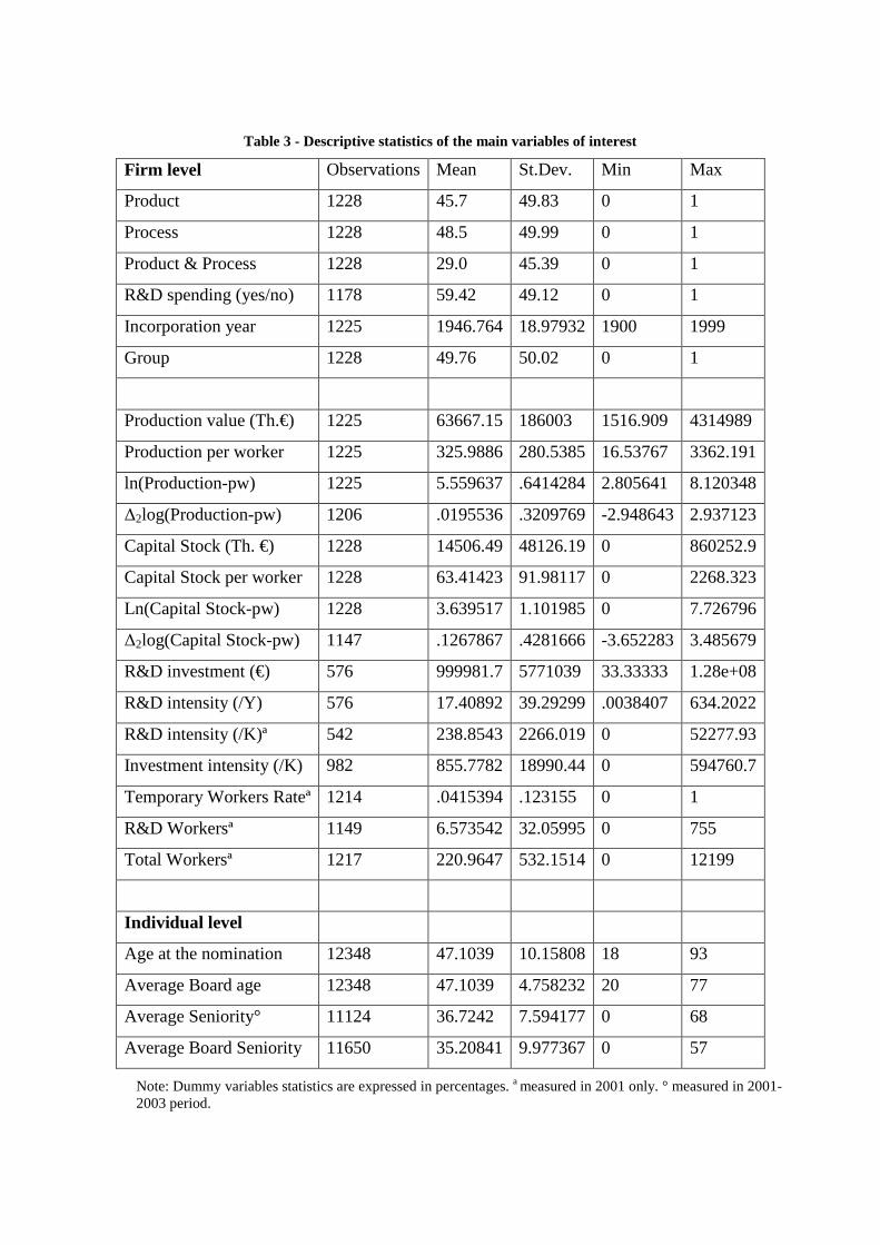
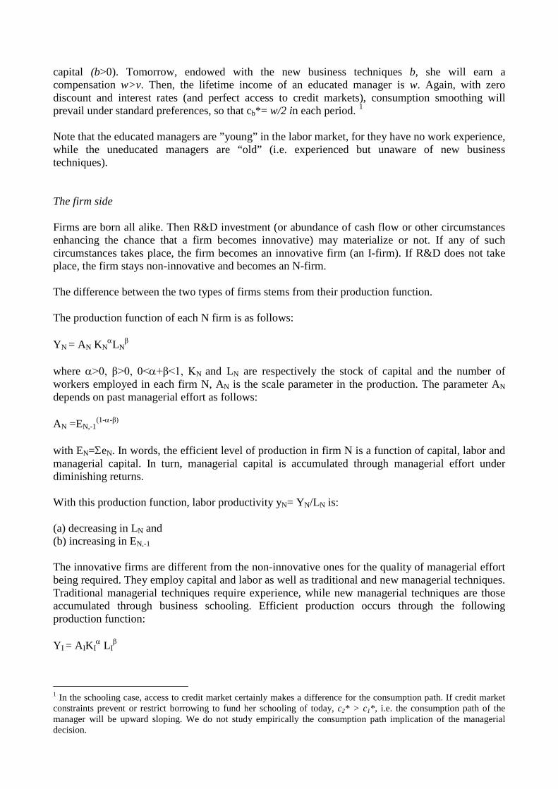
Table 3 - Descriptive statistics of the main variables of interest

Firm level Observations Mean St.Dev. Min Max

Product 1228 45.7 49.83 0 1

Process 1228 48.5 49.99 0 1

Product & Process 1228 29.0 45.39 0 1

R&D spending (yes/no) 1178 59.42 49.12 0 1

Incorporation year 1225 1946.764 18.97932 1900 1999

Group 1228 49.76 50.02 0 1

Production value (Th.€) 1225 63667.15 186003 1516.909 4314989

Production per worker 1225 325.9886 280.5385 16.53767 3362.191

ln(Production-pw) 1225 5.559637 .6414284 2.805641 8.120348

Δ2log(Production-pw) 1206 .0195536 .3209769 -2.948643 2.937123

Capital Stock (Th. €) 1228 14506.49 48126.19 0 860252.9

Capital Stock per worker 1228 63.41423 91.98117 0 2268.323

Ln(Capital Stock-pw) 1228 3.639517 1.101985 0 7.726796

Δ2log(Capital Stock-pw) 1147 .1267867 .4281666 -3.652283 3.485679

R&D investment (€) 576 999981.7 5771039 33.33333 1.28e+08

R&D intensity (/Y) 576 17.40892 39.29299 .0038407 634.2022

R&D intensity (/K)ª 542 238.8543 2266.019 0 52277.93

Investment intensity (/K) 982 855.7782 18990.44 0 594760.7

Temporary Workers Rateª 1214 .0415394 .123155 0 1

R&D Workersª 1149 6.573542 32.05995 0 755

Total Workersª 1217 220.9647 532.1514 0 12199

Individual level

Age at the nomination 12348 47.1039 10.15808 18 93

Average Board age 12348 47.1039 4.758232 20 77

Average Seniority° 11124 36.7242 7.594177 0 68

Average Board Seniority 11650 35.20841 9.977367 0 57

Note: Dummy variables statistics are expressed in percentages. a measured in 2001 only. ° measured in 2001-2003 period.

Firms in the Capitalia dataset (with info in 2001-2003) existing also in 2007 to match AIDA

information are 3562 (that is 85.3% of the sample). Firm-individual observations are 21081. We

first test for potential sample selection of these firms, in terms of age, size, location and sector of

production (younger, bigger or particular sectors could have a higher survival rate, higher

productivity or innovation capacity). The discussion of the potential selection bias is placed in the –

Appendix section. The data then need a cleaning procedure because of inconsistencies between

birth dates and nomination dates of the individual board members. Only 12348 (58.6% of total

observations) distributed in 1228 firms contain sensible information on birth and service dates,

which finally becomes our longitudinal or “quasi”-panel dataset with firms as units and board

members as the longitudinal dimension, in the years 2001-2003.

Table 4 - Firm size and area distribution in the final sample

Small Medium Large North West North East Centre South

Freq 255 730 243 431 407 191 199

% 20.77 59.45 19.79 35.1 33.14 15.55 16.21

6. Estimation results and comments Table 5 shows the OLS coefficients and robust standard errors of the estimates of labor productivity growth rates (2-year rates) on our variables of interest (equation 2), interacted with the group dummies. Column 1 and 2 refer to innovative firms in general (D1 = group of firms introducing a product or process innovation in the 2001-2003 period, D2 = group of non innovative firms). Column 3 and 4 refer to product innovative firms (D1 = group of firms introducing a product innovation) and column 5 and 6 refer to process innovative firms (D1 = group of firms introducing a process innovation). Table 5 - OLS Estimates of Labor Productivity (long) growth rates

Dependent variable

it

it

LY

ln2∆

all innovations Product Process Coefficient Robust

Std. Err. Coefficient Robust

Std. Err. Coefficient

Robust Std. Err.

it

it

LK

ln2∆ .206*** .0195 .2071*** .0191 .2042*** .0194

Innovative firms .350*** .0693 .159*** .0503 .357*** .0527 Age*Innov -.003*** .0004 -.0031*** .0006 -.0043*** .0005 Age*non_Innov .0026** .0013 -.0004 .0008 .0017** .0009 Senior*Innov .0009 .0016 .00039 .0017 .0009 .0016 Senior*non_Innov .0027* .0016 .00159 .0016 .0027* .0016 Temporary*Innov -.194*** .0322 -.2042*** .0386 -.1979*** .0367 Temporary*non_Innov -.126 .0917 -.1420** .0700 -.1295* .0734 Small -.090*** .0098 -.0879*** .0098 -.0896*** .0098 Medium -.099*** .0087 -.0986*** .0087 -.0996*** .0086 Group .043*** .0063 .0419*** .0063 .0445*** .0063 Constant -.148 .1097 .0462 .0869 -.1156 .0964 Semi-elasticity of: Age -.0007 .0014 -.0036 *** .0011 -.0026** .0011 Seniority .0036 .0032 .0020 .0032 .0035 .0031 Temporary share -.320*** .0978 -.346*** .0808 -.327*** .0827 Chow test for instability F(32,12348) 16.98 [0.000] 17.63 [0.000] 19.75 [0.000] Wald test for: Age [0.000] [0.005] [0.000] Seniority [0.000] [0.0024] [0.000] Temporary share [0.484] [0.4319] [0.400] R2 0.1271 0.1256 0.1271 N 12412 12412 12412 Note: * 10%, ** 5%, *** 1% level of significance, p-values in brackets. Size, areas, industry and group dummies are included in all regressions.

The innovation dummy reports a coefficient of 0.35 with high statistical significance. This means that there exists a significant drift for productivity growth for the Italian innovative firms, even in the years considered. This is particularly true for those firms introducing process innovation, while the drift is nearly half that size for those firms introducing product innovation. For the group of innovative firms (column 1) the estimate of the age coefficient is negative and statistically significant, while it takes opposite sign for the non innovative group. Having a younger board of governor on average spurs productivity for currently innovative firms. It appears that an older board is associated to higher productivity in (currently) non innovative firms. The semi-elasticity for the whole sample is instead not significantly different from zero. If we define innovativeness by “product” innovation, then we obtain the results of columns 3-4. The difference here is that average board age seems not to be of any importance for non innovative firms. The semi-elasticity for the whole sample is equal to -0.36 and is statistically significant. When process innovation is taken into account (see column 5-6), the impact of the average board age on productivity is -0.43% for innovative firms, and +0.17% for non-innovative firms. The semi-elasticity for the whole sample is equal to -0.26% and is statistically significant. The coefficient of seniority is zero for the innovative and slightly positive for the non innovative group of firms, both with general innovation and process innovation. The elasticity for the whole sample is not significantly different from zero as well in all columns. The coefficient estimate for the temporary workers share is statistically significant and negative (-0.194) for the innovative group but zero for the non innovative one (it is -0.204 for product innovative firms and -0.142 for firms which have not introduced any product innovation). The elasticity for the whole sample is negative and significant (-0.32). The negative value for age coefficient turns out to be mostly driven by firms undertaking process innovation. Firms which do not introduce process innovation show instead significantly positive coefficients for age and seniority. The presence of older and more senior board members appears to be associated with higher productivity in firms which do not innovate. Young members are associated with higher productivity in innovative firms, while seniority does not seem to matter. The distinction between the group of innovative and non innovative firms is instead immaterial for the share of temporary workers. Having a higher rate of temporary workers is always associated with lower productivity. To confirm our results, Table 5 reports p-values of the Wald tests of parameter instability for the H0 hypotheses:

===

21

21

21

0 :µµλλγγ

H

The test for Age coefficient (γ) rejects the null of equal parameters (p-value of the test is equal to zero). The test for Seniority (λ) rejects the null as well, even for product innovation (whose p-value is < 0.01). This means that the two groups of firms behave differently on these aspects. The test for the share of temporary workers (µ) cannot reject the null of equality: this means that the estimated coefficients do not vary across groups. In general the three Chow tests reveal that the constrained model has to be rejected.

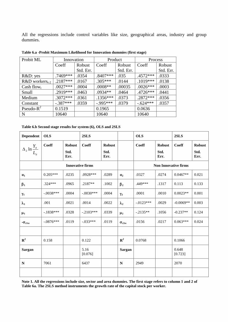
All the regressions include control variables like size, geographical areas, industry and group dummies. Table 6.a -Probit Maximum Likelihood for Innovation dummies (first stage)

Probit ML Innovation Product Process Coeff Robust

Std. Err. Coeff Robust

Std. Err. Coeff

Robust Std. Err.

R&D: yes .7469*** .0354 .8407*** .035 .4572*** .0333 R&D workerst-2 .2187*** .0167 .305*** .0144 .1019*** .0138 Cash flowt .0027*** .0004 .0008** .00035 .0026*** .0003 Small .2919*** .0463 .0934** .0464 .4726*** .0441 Medium .3072*** .0361 .1356*** .0373 .2872*** .0356 Constant -.387*** .0359 -.995*** .0379 -.624*** .0357 Pseudo-R2 0.1519 0.1965 0.0636 N 10640 10640 10640 Table 6.b Second stage results for system (6), OLS and 2SLS

Dependent OLS 2SLS OLS 2SLS

it

it

LY

ln2∆ Coeff Robust

Std. Err.

Coeff Robust

Std. Err.

Coeff Robust

Std. Err.

Coeff Robust

Std. Err.

Innovative firms Non Innovative firms

α1 0.205*** .0235 .0928*** .0289 α2 .0327 .0274 0.0467** 0.021

β1 .324*** .0965 .2187** .1002 β2 .449*** .1317 0.113 0.133

γ1 -.0038*** .0004 -.0030*** .0004 γ2 .0001 .0010 0.0023** 0.001

λ1 .001 .0021 .0014 .0022 λ2 -.0123*** .0029 -0.0069** 0.003

µ1 -.1838*** .0328 -.2103*** .0339 µ2 -.2135** .1056 -0.237** 0.124

-σε1ω -.0876*** .0119 -.033*** .0119 σε2ω .0156 .0217 0.063*** 0.024

R2 0.158 0.122 R2 0.0768 0.1066

Sargan 5.16 [0.076]

Sargan 0.648 [0.723]

N 7061 6437 N 2949 2070

Note 1. All the regressions include size, sector and area dummies. The first stage refers to column 1 and 2 of Table 6a. The 2SLS method instruments the growth rate of the capital stock per worker.

Table 6.a and Table 6.b show the 2-stage method of estimation of the parameters in (4) and (6), which take into account the endogenous formation of the two groups. Table 6.a shows the estimates of the first stage decision to innovate. The probit estimations of Table 6.a are used as a first stage in the switching regression with endogenous switching (eq. (4)). We add the probit for product innovation in columns 3 and 4 or process innovation in columns 5 and 6. These last regressions are useful to understand the importance of the instruments in determining the decision of innovating. For example, engaging into R&D activity and hiring R&D workers have a bigger impact on product innovation than process innovation. Per worker current Cash flow is an important dimension for introducing process innovations. Table 6.b shows the estimates of the second stage switching regression: the Maddala method with OLS on eq. (6) and a 2SLS method to take into account the endogeneity of the growth rate of capital stock per worker.4

The instruments used for the growth rate of the capital stock prediction are the initial level of the capital/labor ratio, age of the firm at the beginning of the sample period, investment intensity at the beginning of the sample period, size, area and sector dummies.

The first comment over Table 6.b regards the fact that close coefficients are obtained for the three main variables of interest, when using OLS and 2SLS methods on the sample of innovative firms. The OLS has a slightly higher R2 though (0.158), and the Sargan test for over-identifying restrictions cannot reject the hypothesis of validity of instruments at the 5% level [p-value of the Sargan test = 0.076]. The impact of mean age of the board members on productivity growth is negative and statistically significant (γ1,OLS = -0.0038, γ1,2SLS = -0.003). The impact of mean seniority of the board members is essentially zero. The impact of the share of temporary workers is negative and significant (µ1,OLS = -0.1838, µ1,2SLS = -.2103) for innovative firms. These latter estimates confirm the results of Table 5. The correction for switching regression is negative and significant (-σε1ω, OLS = -0.0876). The OLS estimate of the capital share appears overestimated (α1,OLS = 0.205) while it is equal to 0.0928 when the capital stock is instrumented. If we compare the OLS and the 2SLS results for the sample of non innovative firms, the results differ in some aspects. The 2SLS method gives a slightly higher R2 (0.1066) and the Sargan test cannot reject the validity of the instruments (p-value = 0.723). The OLS coefficient for the capital stock growth is zero, while it is halved in 2SLS compared to the result for innovative firms (α2 = 0.0467). The impact of the mean Age is null according to OLS, and positive and significant with 2SLS (γ2 = 0.0023). This latter result is coherent with that of Table 5.

4 We run similar regressions of equations (7) and (8) which allows to test for parameters equality between the two regimes. The results confirm the presence of significant differences in the estimates of the coefficients, in particular as far as Seniority and the rate of Temporary workers are concerned, between the two regimes. Table with these other regressions are available upon requests.

The impact of mean seniority is negative and quite significant with both methods (λ2,OLS = -0.0123, λ2,2SLS = -0.0069). This result is opposite with respect to that of Table 5. The impact of the share of temporary workers do not differ significantly across the methods (µ2,OLS = -0.2135, µ2,2SLS = -0.2368) and it is negative and significant. This result differs from that of Table 5 where the correspondent coefficient is zero. The correction for switching regression is not statistically significant for OLS while it is positive and significant for 2SLS (σε2ω,2SLS = 0.063). Notice that the number of observations used with the 2SLS is less than the number of observations in OLS regressions, due to the fact that instrument variables for capital stock contain few more missing values. As a robustness check we replicate the estimates of equation (2) for the sub-sample of managers who are supposed to take decisions within the board. We select those firms whose board contains competence-specific managers, who are supposed to influence the decision to introduce innovations in the firm, eventually. The sign and size of the main coefficients are confirmed.5

We finally implement the Maximum Likelihood Endogenous Switching model which allows us to obtain consistent and efficient estimates. Following the method suggested by Lokshin and Sajaia (2004) we estimate the equation system (3) first by including the growth rate of the capital stock as it is (analogously to the OLS method in Table 6.b), second by substituting the variable with its predicted value obtained through a first-stage regression with instruments (analogously to the 2SLS method used in Table 6.b). The results of the ML Endogenous Switching Model are shown in Table 6.c, below.

5 Results are available upon request.

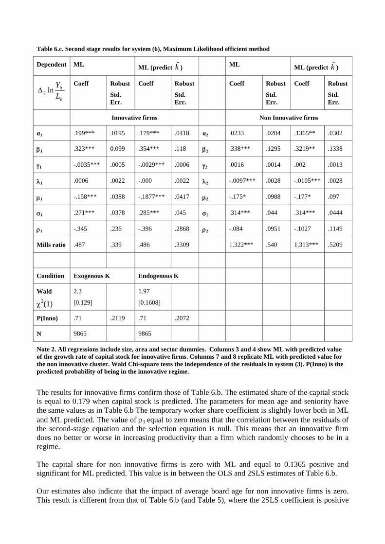
Table 6.c. Second stage results for system (6), Maximum Likelihood efficient method

Dependent ML ML (predict k̂ ) ML ML (predict k̂ )

it

it

LY

ln2∆ Coeff Robust

Std. Err.

Coeff Robust

Std. Err.

Coeff Robust

Std. Err.

Coeff Robust

Std. Err.

Innovative firms Non Innovative firms

α1 .199*** .0195 .179*** .0418 α2 .0233 .0204 .1365** .0302

β1 .323*** 0.099 .354*** .118 β2 .338*** .1295 .3219** .1338

γ1 -.0035*** .0005 -.0029*** .0006 γ2 .0016 .0014 .002 .0013

λ1 .0006 .0022 -.000 .0022 λ2 -.0097*** .0028 -.0105*** .0028

µ1 -.158*** .0388 -.1877*** .0417 µ2 -.175* .0988 -.177* .097

σ1 .271*** .0378 .285*** .045 σ2 .314*** .044 .314*** .0444

ρ1 -.345 .236 -.396 .2868 ρ2 -.084 .0951 -.1027 .1149

Mills ratio .487 .339 .486 .3309 1.322*** .540 1.313*** .5209

Condition Exogenous K Endogenous K

Wald

χ2(1)

2.3

[0.129]

1.97

[0.1608]

P(Inno) .71 .2119 .71 .2072

N 9865 9865

Note 2. All regressions include size, area and sector dummies. Columns 3 and 4 show ML with predicted value of the growth rate of capital stock for innovative firms. Columns 7 and 8 replicate ML with predicted value for the non innovative cluster. Wald Chi-square tests the independence of the residuals in system (3). P(Inno) is the predicted probability of being in the innovative regime.

The results for innovative firms confirm those of Table 6.b. The estimated share of the capital stock is equal to 0.179 when capital stock is predicted. The parameters for mean age and seniority have the same values as in Table 6.b The temporary worker share coefficient is slightly lower both in ML and ML predicted. The value of ρ1 equal to zero means that the correlation between the residuals of the second-stage equation and the selection equation is null. This means that an innovative firm does no better or worse in increasing productivity than a firm which randomly chooses to be in a regime. The capital share for non innovative firms is zero with ML and equal to 0.1365 positive and significant for ML predicted. This value is in between the OLS and 2SLS estimates of Table 6.b. Our estimates also indicate that the impact of average board age for non innovative firms is zero. This result is different from that of Table 6.b (and Table 5), where the 2SLS coefficient is positive

and statistically significant. Seniority is negative and significant for productivity growth of non innovative firms, equivalently to Table 6.b. The impact of the share of temporary workers is negative and significant even if the size of the impact is lower with ML than 2SLS (µ2,ML ≅ µ2,MLpred = -0.175). Finally, the correlation between selecting the regime and the second-stage equation is still zero. This is confirmed by the Wald test of independence across the equations of the system (3). To gain a better understanding of the numerical implications of our results, we take the “ML predicted” as the best coefficients for calculating some exercises of comparative statics. If we evaluate the (absolute value of) elasticity of labor productivity to the mean age of the board members for innovative firms (49.15 years), this is equal to 0.143. This means that a higher age by, say, 10 percent (around 5 years of age) lowers labor productivity by -1.43%, while there would be no productivity change in non-innovative firms. If we evaluate the elasticity of labor productivity with respect to seniority, there would be no impact of a change in seniority spells on productivity for innovative firms. The elasticity for non-innovative firms would be equal to 0.373 at the mean seniority (35.5 years). This means that a higher experience within the firm by 10 percent (around 3 years and a half) would entail a variation of labor productivity by -3.73%, for the non-innovative firms only. Finally the elasticity of labor productivity with respect to the share of temporary workers is equal to 0.0062 for innovative firms, and 0.0057 for non innovative firms (measured at the mean rate values). If the share of temporary workers increases by 10%, then productivity will decrease by 0.62% for innovative firms (on average) and by 0.57% for the non innovative ones.

7. Conclusions Italy’s prolonged productivity slowdown is not a cyclical contingency and deserves careful investigation. In this paper, we give our contribution evaluating two of the main views proposed to explain such slowdown. We find that the Labor Supply view is consistent with our data, while as to the Labor Demand view, our results indicate that managerial experience is not unambiguously correlated with productivity performance in the entire sample. Definite patterns of correlation are present though, once the whole sample is split into innovative and non-innovative clusters. Age, in particular – a measure of overall experience – in the labor market appears to be weakly positively correlated with productivity in non-innovative firms, while it is negatively correlated with productivity for innovative firms. The pattern of correlation for seniority is instead less robust and requires further investigation. The cross-sectional statistical analysis of long-differences based on firm-averaged data is also not problem-free. A big issue is potential reverse causation. The statistical relations we intend to analyze posit that the temporary share of workers, age or seniority variables are the independent variables and productivity the dependent variable. But cross-section data as such (be they observed at a given point in time or averaged over time) may only indicate correlation, not causation. Therefore, if the estimated coefficient linking seniority and productivity is negative, this may not indicate that the firms where aged or senior managers are employed are less productive. Rather, the negative correlation may simply signal that older or senior managers tend to stay longer in less productive and older firms, featuring outdated machines and methods of production, probably because they managed to put in place successful “relations”, while new, innovative and high-productivity plants may be more often matched to young and brilliant managers. If this is the case, we would be wrongly interpreting what causes what, attributing to seniority or age a causal influence on plant productivity, which may go the other way around. This is why we implement our 2SLS specification. Our expectation is that by choosing predetermined instruments we may lessen the simultaneity problems. Surely, a lot of unobserved heterogeneity in plant productivity is still there in the data even once we have augmented the list of productivity determinants with dummies and other control variables. Yet the problem of interpreting the statistical results from cross-sectional estimates arises if and only if the unobserved (therefore unmeasured) firm variables are correlated with the included explanatory variables. For example, if managerial ability – a typically unobserved firm variable – were unrelated to the tenure persistence of managers, then leaving it out of the empirical analysis would not be a major problem. This may or may not be the case though. If managerial ability is not observed and therefore omitted from the analysis but it turns out to be correlated with some included variable such as the tenure persistence of managers, its effect may be picked up by the negative estimated relation between senior managers and productivity. We would be misperceiving the effect of managerial ability on productivity as if it were the causal effect of managerial seniority on productivity. To tackle this problem, we control for a few dummy variables that capture some, though presumably not all, of the unobserved determinants of firm productivity.

References

Bandiera, Oriana, Luigi Guiso, Andrea Prat and Raffaella Sadun (2008), “Italian managers: fidelity or performance?”, Report presented at the Annual Rodolfo De Benedetti Foundation Conference “The ruling class”, Revised: September Crépon Bruno, Duguet E. and Jacques Mairesse (1998), “Research, Innovation and Productivity: an Econometric Analysis at the Firm Level”, NBER Working Paper 6696, Aug. 1998 Daveri, Francesco (2009), “Italy, before and after Lehman Brothers”, VoxEu.org, June 5 Daveri Francesco and Cecilia Jona Lasinio (2005), “Italy’s decline: getting the facts right”, Giornale degli Economisti ed Annali di Economia, December, 365-410 Daveri Francesco and Mika Maliranta (2007), Age, seniority and labour costs: lessons from the Finnish IT revolution”, Economic Policy, 118-175 Gordon Robert J. and Ian Dew-Becker (2008), “The role of labor market changes in the slowdown of European productivity growth”, CEPR Discussion Paper, February 2008 Griliches Zvi (1979), “Issues in assessing the contribution of research and development to productivity growth”, The Bell Journal of Economics, 92-116 Hall Bronwyn, Francesca Lotti and Jacques Mairesse “Employment, innovation and productivity: evidence from Italian microdata”, Industrial and Corporate Change, 2008 Hall Bronwyn, Jacques Mairesse, Louis Branstetter and Bruno Crépon, “Does cash flow cause Investment and R&D: An Exploration Using Panel Data for French, Japanese and United States Scientific Firms”, Discussion Paper Nuffield College Oxford n°142, 1998 Lokshin Michael and Zurab Sajaia (2004): Maximum-likelihood estimation of endogenous switching regression models, Stata-journal, vol. 4, n.3, pp. 282-289 Maddala, G., (1983) Limited-Dependent and Qualitative Variables in Econometric, Econometric Society Monographs No. 3, Cambridge University Press, New York Parisi Maria Laura, Fabio Schiantarelli and Alessandro Sembenelli, “Productivity, Innovation and R&D: Micro Evidence for Italy”, European Economic Review, 2006, 2037–2061

Appendix We control for sample selection that could actually come up when Capitalia IX survey data are matched with AIDA balance sheet of firms present in 2007. Not all Capitalia firms exist in AIDA register. Nonetheless, we manage to retain almost 86% of the Capitalia sample. Therefore, we check in what type of characteristics do firms in-sample and out-of-sample differ.

Figure A 1. In and Out Sample distribution of Capitalia firms by size

0.1

.2.3

.4Fr

actio

n of

firm

s

11-20 21-50 51-250 251-499 500 e oltreSize intervals

out-of-sample in-sample

Firm distribution by number of workers in and out-sample

Figure A1 shows the distribution by class of workers of the firms falling in and out of our final panel. The panel tends to maintain medium size firms mainly (87%), while keeping around 79% of the medium-large and large firms. As far as the very small firms, our panel keeps 82% of them. Formally, the test for independence hypothesis rejects the null (Pearson chi-square(4) = 25.7455, p-value = 0.000) meaning that being in or out of sample depends in a certain way on firm size. We lose 15.6% of firms located in North-West part of Italy (Lombardia, Piemonte, Liguria, Valle d’Aosta), 13.9% of the firms located in the North-East (Trentino A.A., Veneto, Friuli V.G., Emilia Romagna), 13.5% of the firms located in the Centre (Toscana, Umbria, Marche, Lazio) and 15.8% of the firms located in the South. The Pearson chi-square(4) = 3.4150 with p-value = 0.491 says that there is statistical independence between the regional distribution and being in or out of sample. Traditional sectors with lower Ateco 1991 code, i.e. Food and Beverages, Textiles, Clothes, Tobacco, tend to be underrepresented with respect to the original Capitalia sample, as we can see from Figure A2. In any case if we consider High-Tech versus the others, there is an independent distribution of frequencies in and out of sample (Pearson chi-square(1) test = 0.3952 with p-value=0.530).

Figure A 2. Distribution of firms by Ateco 1991 classification, in and out-sample

0.0

5.1

.15

Frac

tion

15 16 17 18 19 20 21 22 23 24 25 26 27 28 29 30 31 32 33 34 35 36 37Ateco 1991

out of sample in-sample

Distribution of firms by Sectors in and out of sample

We then run a two-sample t test with equal variances to test for equality of average firm age between the two groups (in-sample, out-sample). The results highlight that firms outside the sample are on average 3 years older, and the difference in means is statistically significant. Group Obs Mean Std. Err. Std. Dev. [95% Conf. Interval] Out sample 570 31.87 .938 22.41 30.03 33.72 In sample 3469 28.87 .325 19.16 28.24 29.51 Combined 4039 29.29 .309 19.67 28.69 29.90 diff 3.00 .887 1.259 4.742 Degrees of freedom: 4037

Ho: mean(out) - mean(in) = diff = 0

Ha: diff < 0 Ha: diff ≠ 0 Ha: diff > 0 t = 3.3795 t = 3.3795 t = 3.3795

P < t = 0.9996 P > |t| = 0.0007 P > t = 0.0004 Finally, we run an association tests to check for independence between being an innovative firm and being in or out of sample, to evaluate whether less innovative firms are those kicked out of the final panel. The Pearson chi-square tests are listed for different types of innovation activity:

R&D expenditures in 2001-2003 (yes/no)

Pearson chi-square(1) = 3.52 p-value = 0.061

Introducing product innovations (yes/no)

Pearson chi-square(1) = 7.194 p-value = 0.007

Introducing process innovations (yes/no)

Pearson chi-square(1) = 2.189 p-value = 0.139

Introducing both process and product innovations (yes/no)

Pearson chi-square(1) = 2.249 p-value = 0.134

We reject the hypothesis of independence for R&D expenditure and product innovation only. That means that firms investing into R&D and introducing product innovations have a (slightly) higher probability to survive. We cannot reject the null for process innovations or both kinds of innovations, instead. Introducing process innovations or not provide a firm equal probability to remain in our sample.