IEOR E4703: Monte-Carlo SimulationFurther Variance Reduction Methods

Martin HaughDepartment of Industrial Engineering and Operations Research

Columbia UniversityEmail: martin.b.haugh@gmail.com

Outline

Importance SamplingIntroduction and Main ResultsTilted DensitiesEstimating Conditional Expectations

An Application to Portfolio Credit RiskIndependent Default IndicatorsDependent Default Indicators

Stratified SamplingThe Stratified Sampling AlgorithmSome Applications to Option Pricing

2 (Section 0)

Just How Unlucky is a 25 Standard Deviation Return?

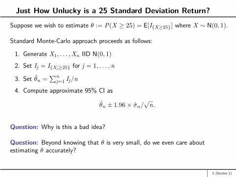
Suppose we wish to estimate θ := P(X ≥ 25) = E[IX≥25] where X ∼ N(0, 1).

Standard Monte-Carlo approach proceeds as follows:

1. Generate X1, . . . ,Xn IID N(0, 1)

2. Set Ij = IXj≥25 for j = 1, . . . ,n

3. Set θn =∑n

j=1 Ij/n

4. Compute approximate 95% CI as

θn ± 1.96× σn/√

n.

Question: Why is this a bad idea?

Question: Beyond knowing that θ is very small, do we even care aboutestimating θ accurately?

3 (Section 1)

The Importance Sampling EstimatorSuppose we wish to estimate θ = Ef [h(X)] where X has PDF f .

Let g be another PDF with the property that g(x) 6= 0 whenever f (x) 6= 0. Then

θ = Ef [h(X)] =∫

h(x) f (x)g(x)g(x) dx = Eg

[h(X)f (X)

g(X)

]- has very important implications for estimating θ.

Original simulation method generates n samples of X from f and setsθn =

∑h(Xj)/n.

Alternative method is to generate n values of X from g and set

θn,is =n∑

j=1

h(Xj)f (Xj)ng(Xj)

.

4 (Section 1)

The Importance Sampling Estimatorθn,is is then an unbiased estimator of θ.

We often defineh∗(X) := h(X)f (X)

g(X)– so that θ = Eg[h∗(X)].

We refer to f and g as the original and importance sampling densities,respectively.

Also refer to f /g as the likelihood ratio.

5 (Section 1)

Just How Unlucky is a 25 Standard Deviation Return?

Recall we want to estimate θ = P(X ≥ 25) = E[IX≥25] when X ∼ N(0, 1).

We write

θ = E[IX≥25] =∫ ∞−∞

IX≥251√2π

e− x22 dx

=∫ ∞−∞

IX≥25

1√2π e− x2

2

1√2π e−

(x−µ)22

1√2π

e−(x−µ)2

2 dx

= Eµ[IX≥25e−µX+µ2/2

]and where now X ∼ N(µ, 1).

Leads to a much more efficient estimator if say we take µ ≈ 25.

Find an approx. 95% CI for θ is given by [3.053, 3.074]× 10−138.

6 (Section 1)

The General FormulationLet X = (X1, . . . ,Xn) be a random vector with joint PDF f (x1, . . . , xn).

Suppose we wish to estimate θ = Ef [h(X)].

Let g(x1, . . . , xn) be another PDF such that g(x) 6= 0 whenever f (x) 6= 0. Then

θ = Ef [h(X)]= Eg[h∗(X)]

where h∗(X) := h(X)f (X)/g(X).

7 (Section 1)

Obtaining a Variance ReductionWe wish to estimate θ = Ef [h(X)] where X is a random vector with joint PDF,f .

We assume wlog (why?) that h(X) ≥ 0.

Now let g be another density with support equal to that of f .

Then we knowθ = Ef [h(X)] = Eg[h∗(X)]

and this gives rise to two estimators:

1. h(X) where X ∼ f

2. h∗(X) where X ∼ g

8 (Section 1)

Obtaining a Variance ReductionThe variance of importance sampling estimator is given by

Varg(h∗(X)) =∫

h∗(x)2g(x) dx − θ2

=∫ h(x)2f (x)

g(x) f (x) dx − θ2.

Variance of original estimator is given by

Varf (h(X)) =∫

h(x)2f (x) dx − θ2.

So reduction in variance is

Varf (h(X))− Varg(h∗(X)) =∫

h(x)2(

1− f (x)g(x)

)f (x) dx.

– would like this reduction to be positive.9 (Section 1)

Obtaining a Variance ReductionFor this to happen, we would like

1. f (x)/g(x) > 1 when h(x)2f (x) is small

2. f (x)/g(x) < 1 when h(x)2f (x) is large.

Could define important part of f to be that region, A say, in the support of fwhere h(x)2f (x) is large.

But by the above observation, would like to choose g so that f (x)/g(x) is smallwhenever x is in A

- that is, we would like a density, g, that puts more weight on A- hence the term importance sampling.

When h involves a rare event so that h(x) = 0 over “most" of the state space, itcan then be particularly valuable to choose g so that we sample often from thatpart of the state space where h(x) 6= 0.

10 (Section 1)

Obtaining a Variance ReductionThis is why importance sampling is most useful for simulating rare events.

Further guidance on how to choose g is obtained from the following observation:

Suppose we choose g(x) = h(x)f (x)/θ.Then easy to see that

Varg(h∗(X)) = θ2 − θ2 = 0

so that we have a zero variance estimator!Would only need one sample with this choice of g.

Of course this is not feasible in practice. Why?

But this observation can often guide us towards excellent choices of g that leadto extremely large variance reductions.

11 (Section 1)

The Maximum PrincipleSaw that if we could choose g(x) = h(x)f (x)/θ, then we would obtain the bestpossible estimator of θ, i.e. a zero-variance estimator.

This suggests that if we could choose g ≈ hf , then might reasonably expect toobtain a large variance reduction.

One possibility is to choose g so that it has a similar shape to hf .

In particular, could choose g so that g(x) and h(x)f (x) both take on theirmaximum values at the same value, x∗, say

- when we choose g this way, we are applying the maximum principle.

Of course this only partially defines g as there are infinitely many densityfunctions that could take their maximum value at x∗.

Nevertheless, often enough to obtain a significant variance reduction.

In practice, often take g to be from the same family of distributions as f .12 (Section 1)

The Maximum Principlee.g. If f is multivariate normal, then might also take g to be multivariate normalbut with a different mean and / or variance-covariance matrix.

We wish to estimate θ = E[h(X)] = E[X4eX2/4IX≥2] where X ∼ N(0, 1).

If we sample from a PDF, g, that is also normal with variance 1 but mean µ,then we know that g takes it maximum value at x = µ.

Therefore, a good choice of µ might be

µ = arg maxx

h(x)f (x) = arg maxx≥2

x4e−x2/4 =√

8.

Thenθ = Eg[h∗(X)] = Eg[X4eX2/4e−

√8X+4IX≥2]

where g(·) denotes the N(√

8, 1) PDF.

13 (Section 1)

Pricing an Asian Optione.g. St ∼ GBM (r , σ2), where St is the stock price at time t.

Want to price an Asian call option whose payoff at time T is given by

h(S) := max(

0,∑m

i=1 SiT/m

m −K)

(1)

where S := SiT/m : i = 1, . . . ,m and K is the strike price.

The price of this option is then given by Ca = EQ0 [e−rTh(S)].

Can writeSiT/m = S0e(r−σ2/2) iT

m +σ√

Tm (X1+...+Xi)

where the Xi ’s are IID N(0, 1).

If f is the risk-neutral PDF of X = (X1, . . . ,Xm), then (with mild abuse ofnotation) may write

Ca = Ef [h(X1, . . . ,Xn)].

14 (Section 1)

Pricing an Asian OptionIf K very large relative to S0 then the option is deep out-of-the-money and usingsimulation amounts to performing a rare event simulation.

As a result, estimating Ca using importance sampling will often result in a largevariance reduction.

To apply importance sampling, we need to choose the sampling density, g.

Could take g to be multivariate normal with variance-covariance matrix equal tothe identity, Im, and mean vector, µ∗

- that is we shift f (x) by µ∗.

As before, a good possible value of µ∗ might be µ∗ = arg maxx h(x)f (x)- can be found using numerical methods.

15 (Section 1)

Potential Problems with the Maximum PrincipleSometimes applying the maximum principle to choose g is difficult.

For example, it may be the case that there are multiple or even infinitely manysolutions to µ∗ = arg maxx h(x)f (x).

Even when there is a unique solution, it may be the case that finding it is verydifficult.

In such circumstances, an alternative method for choosing g is to scale f .

16 (Section 1)

Difficulties with Importance SamplingMost difficult aspect to importance sampling is in choosing a good samplingdensity, g.

In general, need to be very careful for it is possible to choose g according to somegood heuristic such as the maximum principle, but to then find that g results in avariance increase.

Possible in factto choose a g that results in an importance sampling estimatorthat has an infinite variance!

This situation would typically occur when g puts too little weight relative to f onthe tails of the distribution.

In more sophisticated applications of importance sampling it is desirable to have(or prove) some guarantee that the importance sampling variance will be finite.

17 (Section 1)

Tilted DensitiesSuppose f is light-tailed so that it has a moment generating function (MGF).

Then a common way of generating the sampling density, g, from the originaldensity, f , is to use the MGF of f .

Let Mx(t) := E[etX ] denote the MGF.

Then for −∞ < t <∞, a tilted density of f is given by

ft(x) = etx f (x)Mx(t) .

If we want to sample more often from region where X tends to be large (andpositive), then could use ft with t > 0 as our sampling density g.

Similarly, if we want to sample more often from the region where X tends to belarge (and negative), then could use ft with t < 0.

18 (Section 1)

An Example: Sums of Independent Random Variables

Suppose X1, . . . ,Xn are independent r. vars, where Xi has density fi(·).

Let Sn :=∑n

i=1 Xi and want to estimate θ := P(Sn ≥ a) for some constant, a.

If a is large then can use importance sampling.

Since Sn is large when Xi ’s are large it makes sense to sample each Xi from itstilted density function, fi,t(·) for some value of t > 0.

May then write

θ = E[ISn≥a] = Et

[ISn≥a

n∏i=1

fi(Xi)fi,t(Xi)

]

= Et

[ISn≥a

( n∏i=1

Mi(t))

e−tSn

]

where Et [.] denotes expectation with respect to the Xi ’s under the tilteddensities, fi,t(·), and Mi(t) is the moment generating function of Xi .

19 (Section 1)

An Example: Sums of Independent Random Variables

If we write M (t) :=∏n

i=1 Mi(t), then easy to see the importance samplingestimator, θn,i , satisfies

θn,i ≤ M (t)e−ta. (2)

Therefore a good choice of t would be that value that minimizes the bound in (2)

- why is this?

Can minimize the bound by minimizing log(M (t)e−ta) = log(M (t))− ta.

Straightforward to check that minimizing value of t satisfies µt = a whereµt := Et [Sn].

20 (Section 1)

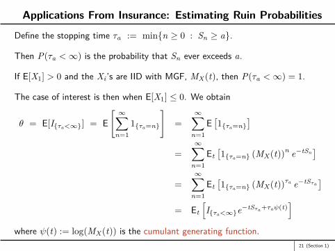
Applications From Insurance: Estimating Ruin Probabilities

Define the stopping time τa := minn ≥ 0 : Sn ≥ a.

Then P(τa <∞) is the probability that Sn ever exceeds a.

If E[X1] > 0 and the Xi ’s are IID with MGF, MX(t), then P(τa <∞) = 1.

The case of interest is then when E[X1] ≤ 0. We obtain

θ = E[Iτa<∞] = E[ ∞∑

n=11τa=n

]=

∞∑n=1

E[1τa=n

]=

∞∑n=1

Et[1τa=n (MX(t))n e−tSn

]=

∞∑n=1

Et[1τa=n (MX(t))τa e−tSτa

]= Et

[Iτa<∞e

−tSτa +τaψ(t)]

where ψ(t) := log(MX(t)) is the cumulant generating function.21 (Section 1)

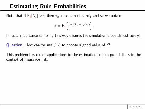
Estimating Ruin ProbabilitiesNote that if Et [X1] > 0 then τa <∞ almost surely and so we obtain

θ = Et

[e−tSτa +τaψ(t)

].

In fact, importance sampling this way ensures the simulation stops almost surely!

Question: How can we use ψ(·) to choose a good value of t?

This problem has direct applications to the estimation of ruin probabilities in thecontext of insurance risk.

22 (Section 1)

Estimating Ruin Probabilitiese.g. Suppose Xi := Yi − cTi where:

Yi is the size of the ith claim

Ti is the inter-arrival time between claims

c is the premium received per unit time

and a is the initial reserve.

Then θ is the probability that the insurance company ever goes bankrupt.

Only in very simple models is it possible to calculate θ analytically- in general, Monte-Carlo approaches are required.

23 (Section 1)

Estimating Conditional ExpectationsImportance sampling also very useful for computing conditional expectationswhen the event being conditioned upon is a rare event.

e.g. Suppose we wish to estimate θ = E[h(X)|X ∈ A] where A is a rare eventand X is a random vector with PDF, f .

Then the density of X, given that X ∈ A, is

f (x|x ∈ A) = f (x)P(X ∈ A) , for x ∈ A

soθ =

E[h(X)IX∈A]E[IX∈A]

.

Since A is a rare event we would be better off using a sampling density, g, thatmakes A more likely to occur.

Then we would have

θ =Eg[h(X)IX∈Af (X)/g(X)]

Eg[IX∈Af (X)/g(X)] .

24 (Section 1)

Estimating Conditional ExpectationsTo estimate θ using importance sampling, we generate X1, . . . ,Xn with densityg, and set

θn,i =∑n

i=1 h(Xi)IXi∈Af (Xi)/g(Xi)∑ni=1 IXi∈Af (Xi)/g(Xi)

.

In contrast to our usual estimators, θn,i is no longer an average of n IID randomvariables but instead, it is the ratio of two such averages

- has implications for computing approximate confidence intervals for θ- in particular, confidence intervals should now be estimated using bootstrap

techniques.

An obvious application of this methodology in risk management is the estimationof quantities similar to ES or CVaR.

25 (Section 1)

Bernoulli Mixture ModelsDefinition: Let p < m and let Ψ = (Ψ1, . . . ,Ψp)> be a p-dimensional randomvector.Then we say the random vector Y = (Y1, . . . ,Ym)> follows a Bernoulli mixturemodel with factor vector Ψ if there are functions

pi : Rp → [0, 1], 1 ≤ i ≤ m,

such that conditional on Ψ the components of Y are independent Bernoullirandom variables satisfying

P(Yi = 1 | Ψ = ψ) = pi(ψ).

26 (Section 2)

An Application to Portfolio Credit RiskWe consider a portfolio loss of the form L =

∑mi=1 eiYi

ei is the deterministic and positive exposure to the ith credit

Yi is the default indicator with corresponding default probability, pi .

Assume also that Y follows a Bernoulli mixture model.

Want to estimate θ := P(L ≥ c) where c >> E[L].

Note that a good importance sampling distribution for θ should also work well forestimating risk measures associated with the α-tail of the loss distribution whereqα(L) ≈ c.

We begin with the case where the default indicators are independent ...

27 (Section 2)

Case 1: Independent Default IndicatorsDefine Ω to be the state space of Y so that Ω = 0, 1m.

Then

P(y) =m∏

i=1pyi

i (1− pi)1−yi , y ∈ Ω

so that

ML(t) = Ef [etL] =m∏

i=1E[eteiYi ] =

m∏i=1

(pietei + 1− pi

).

Let Qt be the corresponding tilted probability measure so that

Qt(y) = et∑m

i=1eiyi

ML(t) P(y) =m∏

i=1

eteiyi

(pietei + 1− pi)pyi

i (1− pi)1−yi

=m∏

i=1qyi

t,i(1− qt,i)1−yi

where qt,i := pietei/(pietei + 1− pi) is the Qt probability of the ith creditdefaulting.

28 (Section 2)

Case 1: Independent Default IndicatorsNote that the default indicators remain independent Bernoulli random variablesunder Qt .

Since qt,i → 1 as t →∞ and qt,i → 0 as t → −∞ it is clear that we can shiftthe mean of L to any value in (0,

∑mi=1 ei).

The same argument that was used in the partial sum example suggests that weshould take t equal to that value that solves

Et [L] =m∑

i=1qi,tei = c.

This value can be found easily using numerical methods.

29 (Section 2)

Case 2: Dependent Default IndicatorsSuppose now that there is a p-dimensional factor vector, Ψ.

We assume the default indicators are independent with default probabilities pi(ψ)conditional on Ψ = ψ.

Suppose also that Ψ ∼ MVNp(0,Σ).

The Monte-Carlo scheme for estimating θ is to first simulate Ψ and to thensimulate Y conditional on Ψ.

Can apply importance sampling to the second step using our discussion ofindependent default indicators.

However, can also apply importance sampling to the first step, i.e. the simulationof Ψ.

30 (Section 2)

Case 2: Dependent Default IndicatorsA natural way to do this is to simulate Ψ form the MVNp(µ,Σ) distribution forsome µ ∈ Rp.

Corresponding likelihood ratio, rµ(Ψ), is given by ratio of the two multivariatenormal densities.

It satisfies

rµ(Ψ) =exp

(− 1

2 Ψ>Σ−1Ψ)

exp(− 1

2 (Ψ− µ)>Σ−1(Ψ− µ))

= exp(−µ>Σ−1Ψ + 12µ>Σ−1µ).

31 (Section 2)

Case 2: How Do We Choose µ?Recall the quantity of interest is θ := P(L ≥ c) = E[P(L ≥ c | Ψ)].

Know from earlier discussion that we’d like to choose importance samplingdensity, g∗(Ψ), so that

g∗(Ψ) ∝ P(L ≥ c | Ψ) exp(−12Ψ>Σ−1Ψ). (3)

Of course this is not possible since we do not know P(L ≥ c | Ψ), the veryquantity that we wish to estimate.

Maximum principle applied to the MVNp(µ,Σ) distribution would then suggesttaking µ equal to the value of Ψ which maximizes the rhs of (3).

Not possible to solve this problem exactly as we do not know P(L ≥ c | Ψ)- but numerical methods can be used to find good approximate solutions- See Glasserman and Li (2005) for further details.

32 (Section 2)

The Algorithm for Estimating θ = P(L ≥ c)1. Generate Ψ1, . . . ,Ψn independently from the MVNp(µ,Σ) distribution.

2. For each Ψi estimate P(L ≥ c | Ψ = Ψi) using the importance samplingdistribution that we described in our discussion of independent defaultindicators.

Let θISn1

(Ψi) be the corresponding estimator based on n1 samples.

3. Full importance sampling estimator then given by

θISn = 1

n

n∑i=1

rµ(Ψi) θISn1

(Ψi).

33 (Section 2)

Stratified Sampling: A Motivating ExampleConsider a game show where contestants first pick a ball at random from an urnand then receive a payoff, Y .

The payoff is random and depends on the color of the selected ball so that if thecolor is c then Y is drawn from the PDF, fc.

The urn contains red, green, blue and yellow balls, and each of the four colors isequally likely to be chosen.

The producer of the game show would like to know how much a contestant willwin on average when he plays the game.

To answer this question, she decides to simulate the payoffs of n contestants andtake their average payoff as her estimate.

34 (Section 3)

Stratified Sampling: A Motivating ExamplePayoff, Y , of each contestant is simulated as follows:

1. Simulate a random variable, I , where I is equally likely to take any of thefour values r , g, b and y

2. Simulate Y from the density fI (y).Average payoff, θ := E[Y ], then estimated by

θn :=∑n

j=1 Yj

n .

Now suppose n = 1000, and that a red ball was chosen 246 times, a green ball270 times, a blue ball 226 times and a yellow ball 258 times.

Question: Would this influence your confidence in θn?

Question: What if fg tended to produce very high payoffs and fb tended toproduce very low payoffs?

Question: Is there anything that we could have done to avoid this type ofproblem occurring?

35 (Section 3)

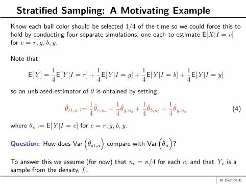
Stratified Sampling: A Motivating ExampleKnow each ball color should be selected 1/4 of the time so we could force this tohold by conducting four separate simulations, one each to estimate E[X |I = c]for c = r , g, b, y.

Note that

E[Y ] = 14E[Y |I = r ] + 1

4E[Y |I = g] + 14E[Y |I = b] + 1

4E[Y |I = y]

so an unbiased estimator of θ is obtained by setting

θst,n := 14 θr,nr + 1

4 θg,ng + 14 θb,nb + 1

4 θy,ny (4)

where θc := E[Y |I = c] for c = r , g, b, y.

Question: How does Var(θst,n

)compare with Var

(θn

)?

To answer this we assume (for now) that nc = n/4 for each c, and that Yc is asample from the density, fc.

36 (Section 3)

Stratified Sampling: A Motivating ExampleThen a fair comparison of Var(θn) with Var(θst,n) should compare

Var(Y1 + Y2 + Y3 + Y4) with Var(Yr + Yg + Yb + Yy) (5)

Y1, Y2, Y3 and Y4 are IID samples from the original simulation algorithm

Yc’s are independent with density fc(·), for c = r , g, b, y.

Now recall the conditional variance formula which states

Var(Y ) = E[Var(Y |I )] + Var(E[Y |I ]). (6)

Each term in the right-hand-side of (6) is non-negative so this implies

Var(Y ) ≥ E[Var(Y |I )]

= 14Var(Y |I = r) + 1

4Var(Y |I = g) + 14Var(Y |I = b) + 1

4Var(Y |I = y)

= Var(Yr + Yg + Yb + Yy)4 .

37 (Section 3)

Stratified SamplingThis implies

Var(Y1 + Y2 + Y3 + Y4) = 4 Var(Y )

≥ Var(Yr + Yg + Yb + Yy).

Can therefore conclude that using θst,n leads to a variance reduction.

Variance reduction will be substantial if I accounts for a large fraction of thevariance of Y .

Note also that computational requirements for computing θst,n are similar tothose required for computing θn.

We call θst,n a stratified sampling estimator of θ and say that I is thestratification variable.

38 (Section 3)

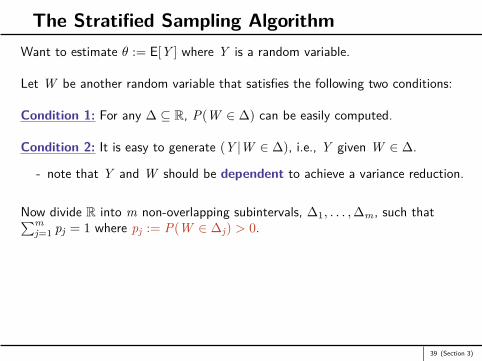
The Stratified Sampling AlgorithmWant to estimate θ := E[Y ] where Y is a random variable.

Let W be another random variable that satisfies the following two conditions:

Condition 1: For any ∆ ⊆ R, P(W ∈ ∆) can be easily computed.

Condition 2: It is easy to generate (Y |W ∈ ∆), i.e., Y given W ∈ ∆.

- note that Y and W should be dependent to achieve a variance reduction.

Now divide R into m non-overlapping subintervals, ∆1, . . . ,∆m, such that∑mj=1 pj = 1 where pj := P(W ∈ ∆j) > 0.

39 (Section 3)

Notation

1. Let θj := E[Y |W ∈ ∆j ] and σ2j := Var(Y |W ∈ ∆j).

2. Define the random variable I by setting I := j if W ∈ ∆j .

3. Let Y (j) denote a random variable with the same distribution as(Y |W ∈ ∆j) ≡ (Y |I = j).

Therefore haveθj = E[Y |I = j] = E[Y (j)]

andσ2

j = Var(Y |I = j) = Var(Y (j)).

40 (Section 3)

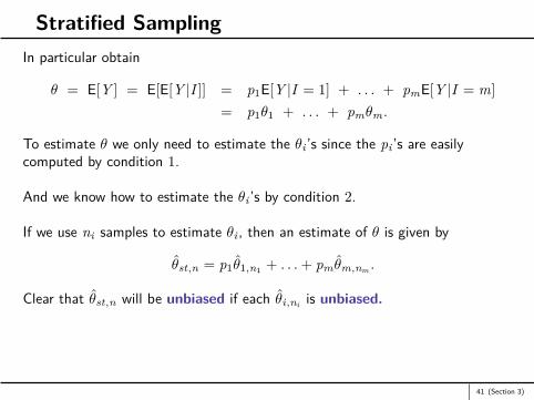
Stratified SamplingIn particular obtain

θ = E[Y ] = E[E[Y |I ]] = p1E[Y |I = 1] + . . . + pmE[Y |I = m]= p1θ1 + . . . + pmθm.

To estimate θ we only need to estimate the θi ’s since the pi ’s are easilycomputed by condition 1.

And we know how to estimate the θi ’s by condition 2.

If we use ni samples to estimate θi , then an estimate of θ is given by

θst,n = p1θ1,n1 + . . .+ pm θm,nm .

Clear that θst,n will be unbiased if each θi,ni is unbiased.

41 (Section 3)

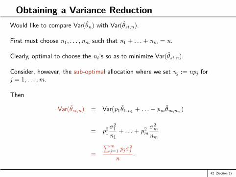
Obtaining a Variance ReductionWould like to compare Var(θn) with Var(θst,n).

First must choose n1, . . . ,nm such that n1 + . . .+ nm = n.

Clearly, optimal to choose the ni ’s so as to minimize Var(θst,n).

Consider, however, the sub-optimal allocation where we set nj := npj forj = 1, . . . ,m.

Then

Var(θst,n) = Var(p1θ1,n1 + . . .+ pm θm,nm )

= p21σ2

1n1

+ . . .+ p2mσ2

mnm

=∑m

j=1 pjσ2j

n .

42 (Section 3)

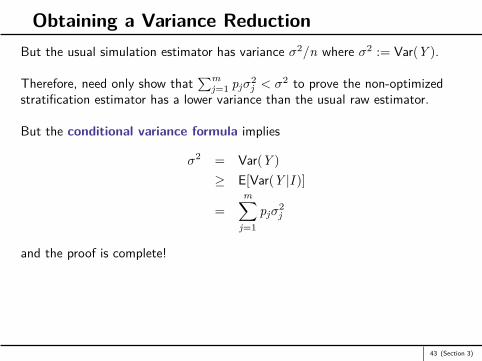
Obtaining a Variance ReductionBut the usual simulation estimator has variance σ2/n where σ2 := Var(Y ).

Therefore, need only show that∑m

j=1 pjσ2j < σ2 to prove the non-optimized

stratification estimator has a lower variance than the usual raw estimator.

But the conditional variance formula implies

σ2 = Var(Y )≥ E[Var(Y |I )]

=m∑

j=1pjσ

2j

and the proof is complete!

43 (Section 3)

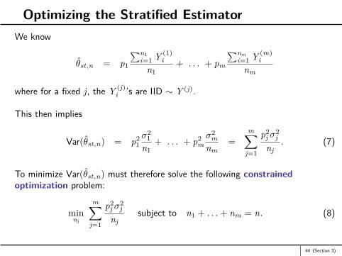
Optimizing the Stratified EstimatorWe know

θst,n = p1

∑n1i=1 Y (1)

in1

+ . . . + pm

∑nmi=1 Y (m)

inm

where for a fixed j, the Y (j)i ’s are IID ∼ Y (j).

This then implies

Var(θst,n) = p21σ2

1n1

+ . . . + p2mσ2

mnm

=m∑

j=1

p2j σ

2j

nj. (7)

To minimize Var(θst,n) must therefore solve the following constrainedoptimization problem:

minnj

m∑j=1

p2j σ

2j

njsubject to n1 + . . .+ nm = n. (8)

44 (Section 3)

Optimizing the Stratified EstimatorCan easily solve (8) using a Lagrange multiplier to obtain

n∗j =(

pjσj∑mj=1 pjσj

)n. (9)

Minimized variance is given by

Var(θst,n∗) =

(∑mj=1 pjσj

)2

n .

Note that the solution (9) makes intuitive sense:

If pj large then (other things being equal) makes sense to expend more effortsimulating from stratum j.

If σ2j is large then (other things being equal) makes sense to simulate more

often from stratum j so as to get a more accurate estimate of θj .

45 (Section 3)

Stratification Simulation Algorithm for Estimating θ

set θn,st = 0; σ2n,st = 0;

for j = 1 to mset sumj = 0; sum_squaresj = 0;for i = 1 to nj

generate Y (j)i

set sumj = sumj + Y (j)i

set sum_squaresj = sum_squaresj + Y (j)i

2

end forset θj = sumj/njset σ2

j =(sum_squaresj − sum2

j /nj)/(nj − 1)

set θn,st = θn,st + pjθjset σ2

n,st = σ2n,st + σ2

j p2j /nj

end forset approx. 100(1− α) % CI = θn,st ± z1−α/2 σn,st

46 (Section 3)

Example: Pricing a European Call OptionWish to price a European call option where we assume St ∼ GBM (r , σ2).

ThenC0 = E

[e−rT max(0,ST −K )

]= E[Y ]

where Y = h(X) = e−rT max(

0, S0e(r−σ2/2)T+σ√

TX −K)

for X ∼ N(0, 1).

While we know how to compute C0 analytically, it’s worthwhile seeing how wecould estimate it using stratified simulation.

Let W = X be our stratification variable. To see that we can stratify using thischoice of W note that:

1. We can easily computed P(W ∈ ∆) for ∆ ⊆ R.

2. We can easily generate (Y |W ∈ ∆).

Therefore clear that we can estimate C0 using X as a stratification variable.

47 (Section 3)

Example: Pricing an Asian Call OptionThe discounted payoff of an Asian call option is given by

Y := e−rT max(

0,∑m

i=1 SiT/m

m −K)

(10)

– its price therefore given by Ca = E[Y ].

Now each SiT/m may be expressed as

SiT/m = S0 exp(

(r − σ2/2) iTm + σ

√Tm (X1 + . . . + Xi)

)(11)

where the Xi ’s are IID N(0, 1).

Can therefore write Ca = E [h(X1, . . . ,Xm)] where h(.) given implicitly by (10)and (11).

48 (Section 3)

Example: Pricing an Asian Call OptionCan estimate Ca using stratified sampling but must first choose a stratificationvariable, W .

One possible choice would be to set W = Xj for some j.

But this is unlikely to capture much of the variability of h(X1, . . . ,Xm).

A much better choice would be to set W =∑m

j=1 Xj .

Of course, we need to show that such a choice is possible, i.e. must show that

(1) P(W ∈ ∆) is easily computed

(2) (Y |W ∈ ∆) is easily generated.

49 (Section 3)

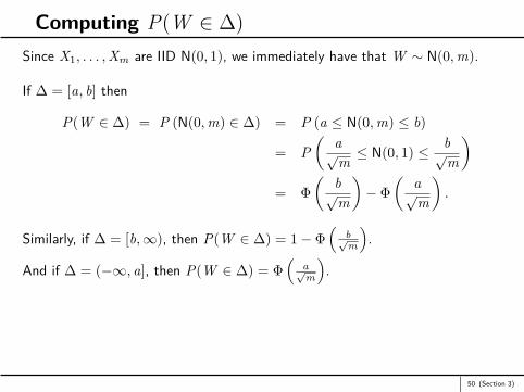
Computing P(W ∈ ∆)Since X1, . . . ,Xm are IID N(0, 1), we immediately have that W ∼ N(0,m).

If ∆ = [a, b] then

P(W ∈ ∆) = P (N(0,m) ∈ ∆) = P (a ≤ N(0,m) ≤ b)

= P(

a√m≤ N(0, 1) ≤ b√

m

)= Φ

(b√m

)− Φ

(a√m

).

Similarly, if ∆ = [b,∞), then P(W ∈ ∆) = 1− Φ(

b√m

).

And if ∆ = (−∞, a], then P(W ∈ ∆) = Φ(

a√m

).

50 (Section 3)

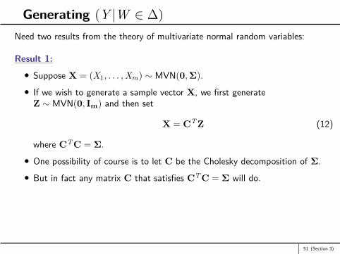
Generating (Y |W ∈ ∆)Need two results from the theory of multivariate normal random variables:

Result 1:

Suppose X = (X1, . . . ,Xm) ∼ MVN(0,Σ).

If we wish to generate a sample vector X, we first generateZ ∼ MVN(0, Im) and then set

X = CTZ (12)

where CTC = Σ.

One possibility of course is to let C be the Cholesky decomposition of Σ.

But in fact any matrix C that satisfies CTC = Σ will do.

51 (Section 3)

Result 2Let a = (a1 a2 . . . am) satisfy ||a|| = 1, i.e.

√a2

1 + . . .+ a2m = 1, and let

Z = (Z1, . . . ,Zm) ∼ MVN(0, Im). Then

(Z1, . . . ,Zm)

∣∣∣ m∑i=1

aiZi = w∼ MVN(wa>, Im − a>a).

Therefore, to generate (Z1, . . . ,Zm)|∑m

i=1 aiZi = w just need to generate Vwhere

V ∼ MVN(wa>, Im − a>a) = wa> + MVN(0, Im − a>a).

Generating such a V is very easy since

(Im − a>a)>(Im − a>a) = Im − a>a.

That is, Σ>Σ = Σ where Σ = Im − a>a

- so we can take C = Σ in (12).

52 (Section 3)

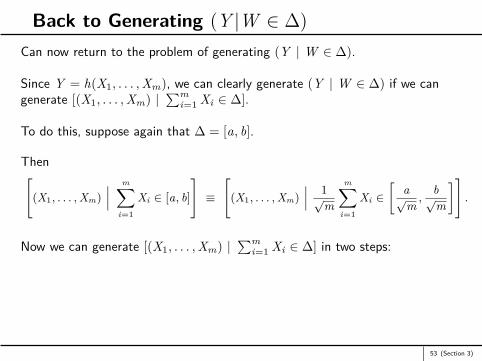
Back to Generating (Y |W ∈ ∆)Can now return to the problem of generating (Y | W ∈ ∆).

Since Y = h(X1, . . . ,Xm), we can clearly generate (Y | W ∈ ∆) if we cangenerate [(X1, . . . ,Xm) |

∑mi=1 Xi ∈ ∆].

To do this, suppose again that ∆ = [a, b].

Then[(X1, . . . , Xm)

∣∣∣ m∑i=1

Xi ∈ [a, b]

]≡

[(X1, . . . , Xm)

∣∣∣ 1√m

m∑i=1

Xi ∈[

a√m

,b√m

]].

Now we can generate [(X1, . . . ,Xm) |∑m

i=1 Xi ∈ ∆] in two steps:

53 (Section 3)

Back to Generating (Y |W ∈ ∆)Step 1: Generate

[1√m∑m

i=1 Xi

∣∣∣ 1√m∑m

i=1 Xi ∈[

a√m ,

b√m

]].

Easy to do since 1√m∑m

i=1 Xi ∼ N(0, 1) so just need to generate(N(0, 1)

∣∣∣ N(0, 1) ∈[

a√m,

b√m

]).

Let w be the generated value.

Step 2:Now generate [

(X1, . . . ,Xm)∣∣∣ 1√

m

m∑i=1

Xi = w]

which we can do by Result 2 and the comments that follow.

54 (Section 3)