IEEE TRANSACTIONS ON VISUALIZATION AND ...chengu/Publications/TVCG11_timedep...IEEE TRANSACTIONS ON VISUALIZATION AND COMPUTER GRAPHICS, VOL., NO., ? 2011 1 Design of 2D Time-Varying

IEEE TRANSACTIONS ON VISUALIZATION AND COMPUTER GRAPHICS, VOL. ?, NO. ?, ? 2011 1

Design of 2D Time-Varying Vector FieldsGuoning Chen, Member, IEEE, Vivek Kwatra, Li-Yi Wei, Charles D. Hansen, Fellow, IEEE, and Eugene

Zhang, Senior Member, IEEE,

Abstract—Design of time-varying vector fields, i.e., vector fields that can change over time, has a wide variety of important applicationsin computer graphics. Existing vector field design techniques do not address time-varying vector fields. In this paper, we present aframework for the design of time-varying vector fields, both for planar domains as well as manifold surfaces. Our system supportsthe creation and modification of various time-varying vector fields with desired spatial and temporal characteristics through severaldesign metaphors, including streamlines, pathlines, singularity paths, and bifurcations. These design metaphors are integrated intoan element-based design to generate the time-varying vector fields via a sequence of basis field summations or spatial constrainedoptimizations at the sampled times. The key frame design and field deformation are also introduced to support other user designscenarios. Accordingly, a spatial-temporal constrained optimization and the time-varying transformation are employed to generate thedesired fields for these two design scenarios, respectively. We apply the time-varying vector fields generated using our design system toa number of important computer graphics applications that require controllable dynamic effects, such as evolving surface appearance,dynamic scene design, steerable crowd movement, and painterly animation. Many of these are difficult or impossible to achieve viaprior simulation-based methods. In these applications, the time-varying vector fields have been applied as either orientation fields oradvection fields to control the instantaneous appearance or evolving trajectories of the dynamic effects.

Index Terms—time-varying vector fields, 2D vector fields, vector field design, dynamic effects for surfaces

F

1 INTRODUCTION

V ECTOR field design is a fundamental component for avariety of graphics applications such as remeshing [1],

[33], texturing [20], [13], [23], [31], [41], [46], and non-photorealistic rendering [16], [17]. The paramount importanceof vector fields in these applications has invoked a line ofcomprehensive study on the techniques of vector field designon surfaces [6], [8], [34], [51]. Nonetheless, prior research haspaid little attention to the more natural and general applicationsof vector field design to modeling dynamic effects, such asfluid animation [35], [36], crowds [4], [29], shape deforma-tion [45], and video editing [18]. This is partly due to the factthat such dynamic systems are usually time-varying (or time-dependent), with the additional time dimension significantlyincreasing the complexity of the possible dynamics in thevector fields. In addition, there is no existing theory for thecharacterization of time-varying vector fields, compared tothe well-defined feature characterization of static vector fieldsupon which the design techniques are built. For the firsttime, this paper systematically studies the design of time-varying vector fields on two-dimensional manifolds, includingthe applications and the taxonomy of the vector fields, therequirements, and the appropriate techniques.

• Guoning Chen and Charles Hansen are with Scientific Computing andImaging Institute, University of Utah, Salt Lake City, UT 84112.E-mail: {chengu,hansen}@sci.utah.edu

• Vivek Kwatra is with Google Inc., Mountain View, CA 94043.E-mail: [email protected]

• Li-Yi Wei is with Microsoft Research, Redmond, WA 98052-6399, and TheUniversity of Hong Kong, Pokfulam, Hong Kong.

• Eugene Zhang is with Oregon State University, Corvallis, OR 97331.E-mail: [email protected]

1.1 Requirements

For most graphics applications involving dynamic effects,there are a number of requirements for the underlying time-varying vector fields and how they are modeled.

First, the obtained time-varying vector fields should preservetemporal coherence to guarantee the smooth transition of thedynamic effects that they are driving. This is a fundamentalrequirement for achieving a visually pleasing animation.

Second, the obtained time-varying vector fields can bephysically plausible or implausible, incompressible or com-pressible, in order to satisfy the requirements of differentapplications. For instance, practitioners in fluid dynamics oftenrequire incompressible flows, while animators may seek formore flexible vector fields for the dynamic effects with volumechange such as crowd simulation. Any vector field systemneeds to be able to handle general time-varying vector fieldswith similarly diverse properties.

Third, the time-varying vector fields are designed to eithercontrol the evolution of the instantaneous appearance of certaingraphical primitives (e.g. the sizes and orientations of thetexture and brush strokes) or advect certain objects (e.g. flowparcels) over time, in order to control different aspects of thedynamic effects. A vector field design system should facilitatethe creation of the vector fields for both types of use.

Fourth, the design system for the time-varying vector fieldsshould provide the user an intuitive and flexible interface tosupport the modeling of various flow behaviors. In addition, anumber of different modeling approaches should be supported.Specifically, there are a few possible situations during themodeling of a time-varying vector field that a user mayencounter: 1) The user wishes to design the detailed localbehavior of the flow over time; 2) The user cares about the


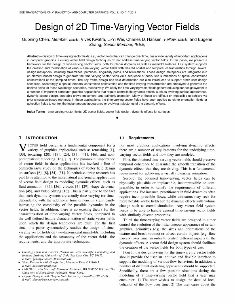
Fig. 1: This figure shows the pipeline of the presented design system for 2D time-varying vector fields. First, the user specifies the desiredflow behaviors in the forms of spatial-temporal constraints. The system then produces a time-varying vector field that matches the constraints.The obtained field is then applied to computer graphics applications to create various dynamic effects. Here, we apply the obtained fields toproduce painterly animation from a single image. Note that we use the created time-varying vector field to orient and move the brush strokesin the lower part of the image to achieve an artistic water wave effect: the vortex rotates, moves and changes its characteristics, then splitsinto two vortices at the end. Please see the accompanying video for this animation. The inset plot shows the changes of the consecutiveinstantaneous fields in terms of the total variance of the vector values in the space.

exact states of the flow at only certain times and wouldlike the system to generate the rest of the field; 3) Theuser is given a static vector field, and tries to deform it tomake up a time-varying vector field as people do for meshdeformation. A properly devised design system should be ableto accommodate these scenarios.

1.2 Our MethodIn order to develop a design system that satisfies the afore-mentioned requirements, we propose a design framework thatis built on the discretization of the time-varying vector fieldsin the time dimension such that they can be considered as thesequences of static vector fields with slow changes over time.This philosophy is based on an observation that solutions to thetime-varying vector fields converge to families of solutions ofthe instantaneous vector fields as the rate of temporal changein the vector field goes to zero, which preserves temporalcoherence and helps achieve smooth transition of the dynamiceffects. This observation is also a fundamental assumptionwhen developing bifurcation theory for time-varying vectorfields [11]. With this temporal discretization, we are able toadapt the previously developed tools for static vector fielddesign to time-varying vector fields with the desired instan-taneous dynamics.

To enable the creation of various flows, we provide the userwith the ability of modeling the following flow properties:

1) a snapshot of the flow at a given time; 2) the path ofa particle in the domain; 3) the path of a singular feature;and 4) the interaction of the features of interest. Thesefeatures in turn reflect important flow characteristics, such asthe solution of the dynamical system at a given time, thetrajectories of the flow parcels, and how the flow parcelsinteract over time. These flow characteristics can be describedby streamlines, pathlines, singularity paths, and bifurcations,respectively. They sufficiently describe the local flow behaviorin space and time, and thus can be used to create time-varyingvector fields for aligning or advecting graphical primitives asrequired. We refer to vector fields that are used for orientinggraphical primitives as orientation fields and advecting objectsas advection fields. We provide the design metaphors forthe user to model these flow characteristics. Particularly, wepresent the first technique that allows the user to prescribebifurcations, a unique type of phenomena not present in staticfields.

To support the required design scenarios, we introduce threedistinct field design approaches. Specifically, the modelingof the local flow behaviors is supported by the time-varyingdesign elements extracted from the user-specified flow charac-teristics. A basis field summation or a constrained optimizationis performed to generate the instantaneous vector field ata given time, based on the instantaneous characteristics ofthe elements. Key-frame design is employed to support the


case when a user only provides the instantaneous fields atthe desired times. A spatial-temporal Laplacian relaxation isproposed to generate the rest of the sequence. Time-varyingtransformation is used when an initial static field is deformedover time to produce a time-varying vector field.

The combination of the proposed design metaphors andgeneration techniques has led to a design system which takesthe user input and generates a time-varying vector field usingone of the generation approaches according to the selecteddesign approach. The system also enables the user to furthermodify the obtained vector field through local topological edit-ing. The generated time-varying vector fields can be appliedto a number of important computer graphics applications toachieve various dynamic effects including producing artisticfluid effects over static images, steering 2D crowds, andcontrolling various time-varying effects on surfaces.

2 RELATED WORK

Vector field design refers to the creation of a continuousvector field on a manifold that respects user-specified orapplication-dependent constraints. Most existing work focuseson a static vector field. Depending on the goals, there are twodifferent classes of vector field design techniques: One is non-topological-based; the other is topological-based.

Non-topological-based methods: Non-topological-basedmethods do not address vector field topology [15] explicitly.The vector field design tools in the early graphics applications,such as texture synthesis [41], [46], fluid simulation [35],[36], and visualization [43], are examples of this category.Other applications, such as non-photorealistic rendering [16],[17], remeshing [1], and parameterization [33], also employvector field design, respectively. Most of these applicationsrequire only the direction information of the input vectorfields, and hence a simple design functionality. However, theuser has little control of unwanted singularities in the fieldthat often lead to visual artifacts.

Topological-based methods: Topological-based approachesallow the user to control the number and positions of singu-larities [44], [51], [8] or the topological graph explicitly [37].General N-way rotational symmetry field design has also beenstudied by Palacios and Zhang [27], Ray et al. [34], and Lai etal. [21]. Recently, Crane et al. [6] present a technique whichallows arbitrary prescription of singularities and constraints onthe fields.

Time-varying methods: Most of the above work concernsonly time-independent (i.e. static) vector fields. On the otherhand, many applications are driven by time-varying vectorfields, such as fluid simulation [35], crowd animation [39],[29], shape deformation [45], hair modeling [10], and videoediting [50]. However, there is no interface that allows the userto intervene the underlying time-varying vector fields. This hasrestricted the achievable effects. Wejchert and Haumann [47]introduce the idea of flow design to create controllable aero-dynamics animation. The modeled field is steady and needsto be combined with physically-based simulation to generateaerodynamics animation. To achieve time-dependent control,

the user exerts external force to the system as demonstratedby Stam [35], [36]. However, simulation is expensive and hardto control. In addition, simulation is incapable of generatingphysically impossible artistic fluid flow effects. Pighin etal. [30] introduce an interactive pathline editing interfaceand an advected radial basis function to model and editincompressible flows. Compared to their work, our techniquesenable the user to create 2D vector fields with more generalcharacteristics than incompressible flows. Kagaya et al. [18]present a design interface to control time-varying tensor fieldsfor the temporarily coherent painterly rendering of videos. Xuet al. [49] describe a technique for fast generation of staticvector fields to assist interactive design. Ma et al. [24] proposea motion field synthesis technique that enables the user togenerate artistic flow effects. However, the method only gen-erates detailed motion vectors and relies on a predeterminedlow resolution dynamic vector field for synthesis. To that end,we are not aware of any work on the design of time-varyingvector fields for the general purpose of graphics applications.

3 OVERVIEWIn this section, we provide a brief description of how ourframework assists the design of a time-varying vector field.First, the user specifies the desired flow characteristics usingthe following flow descriptors:

flow descriptors examples

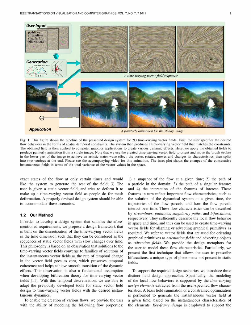
Streamline, for the controlof the flow geometry at acertain time frame and mostuseful for the design of ori-entation fieldsPathline, for the descrip-tion of movements of spe-cific particles across spaceand time (appropriate for ad-vection fields)Singularity path, for therepresentation of the trajec-tory of the singular featuresover space and time (usefulfor orientation fields)Bifurcation, for the descrip-tion of the collisions or splitsof different singular featuresover space and time (usefulfor orientation fields)

These descriptors depict different flow behaviors that canbe observed in many applications. For instance, in texturesynthesis and painterly rendering, the user often wants thetexture patches and brush strokes to be oriented in a certainway. An orientation field can be created to achieve thatwith the desired instantaneous flow patterns prescribed bythe specified streamlines. In crowd simulation, the user wouldlike to steer a group of pedestrians to follow a certain route(or path). An advection field generated from the specifiedpathline can be applied to accomplish that (see Figure 15).


In a meteorological animation, the user may create the effectof two storm systems moving toward each other and eventuallycolliding (see Figure 9). This can be done by controllingthe movement (i.e. singularity paths) and interaction (i.e.bifurcation) of the two vortices in a time-varying vector field.

Note that for most graphics applications shown in this paper,instantaneous appearance is often more important than theexact path of a particle. For the rest of the paper, we willassume the designed fields serve as orientation fields exceptfor the application of crowd simulation where the pathlinedesign is used to generate an advection field. Nonetheless, formost examples the orientation fields are also used to advect thegraphical primitives over time to achieve the effect of motion.

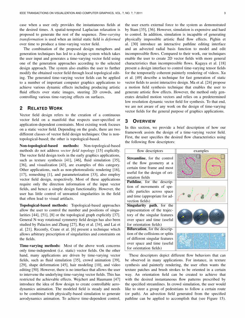
The overall pipeline of our system is as follows (Figure 1).First, according to the selected design scenario, the userspecifies a number of constraints. For key frame design andfield deformation, the focus is the creation of some instan-taneous (static) fields. As such, specifying streamlines andsingularities is sufficient. A streamline can be specified usingthe drawing tool of our system, which will compute the tangentvectors at the sample positions along the streamline as theconstraints. For element-based design, pathlines, singularitypaths, and bifurcations can be designed. In particular, for apathline, besides computing the tangent vectors at the sampledpositions, the temporal value for each sample point is requiredfrom the user (Section 5.1). The user is also responsible forproviding the type for a singularity path (source, sink, orsaddle) as a time-varying Jacobian. To specify a bifurcation,the user can describe a template function (Section 5.1) thatwill create the desired bifurcation. Note that in our system weonly handle saddle-node bifurcation where a node is either asource or sink. Figure 2 provides some examples on how theusers can specify these flow descriptors with our system.

Once the constraints have been specified, our system gener-ates a time-varying vector field by using the basis field sum-mation (Section 5.2), constrained optimization (Sections 5.3and 6.1), or time-varying transformation (Section 7) accordingto the selected design method. The resulting field is analyzedwith singularities and bifurcations extracted. The user then hasthe ability to specify additional constraints or perform localtopological editing in the form of singularity and bifurcationmovement or cancellation. This process continues until theuser is satisfied (Section 8).

In the next section, we will provide the mathematicaldefinitions for the aforementioned flow characteristics.

4 TIME-VARYING VECTOR FIELDS

In this section, we briefly review the important concepts oftime-varying vector fields, which will facilitate our later designtasks.

Streamlines and Pathlines: We consider a 2-manifold M. Atime-varying vector field V is a map V : M×R→M, whichcan be expressed as a differential equation dx

dt = V (x; t). Thesolution of it given an initial state p0 = (x0; t0) is x(b) = p0 +∫ b

0 V (x(η); t0 +η)dη , which is referred to as a pathline. It isthe trajectory of the particle under V . The vector field V (x; tc)is an instantaneous vector field of V at time tc, which is steady.

Fig. 2: Our user interface showing different design metaphors: (a)streamline, (b) pathline, (c) singularity path, and (d) bifurcation. Astreamline is specified at a particular time as a 2D curve. A pathlinecan be provided either in the 2D domain with the starting and endingtime information or directly in the spatial-temporal domain (see theinset of b). Similarly, a singularity path can be designed in either2D domain with the birth and death times or in the spatial-temporaldomain (see the inset of d). A bifurcation is prescribed as a pointin the spatial-temporal domain with the coordinate, scaling, andorientation information.

The solution from pc = (xc; tc) constrained in V (x; tc) is astreamline, and x(b) = pc +

∫ b0 V (x(η); tc)dη .

Instantaneous Topology: The topology of V (x; tc) is referredto as the instantaneous topology of V at tc. It consists ofsingularities, periodic orbits, and their connectivity [3] anddescribes the qualitative information of V (x; tc). This infor-mation has been applied to guide the creation and controlof static vector fields [3], [8], [44], [51]. It has been shownthat analyzing and tracking instantaneous features can providemore information for graphics applications than the space-timetopology based on pathlines that is typically featureless [38].Therefore, in the rest of the paper, we will make use ofthe notion of instantaneous topology to discuss the structuralevolution of a time-varying vector field. Also, we focus onsingularities only as they are relevant to the present graphicsapplications.

Singularities and Singularity Paths: A point p is calleda singularity of V (x; tc) if V (p; tc) = 0. We are interestedin the isolated singularities in the field, each of which canbe enclosed by a compact neighborhood containing no othersingularities. The type of each singularity is determined by theflow characteristics within this neighborhood. The lineariza-tion of V (x; tc) about p results in a 2× 2 matrix DV (p) =


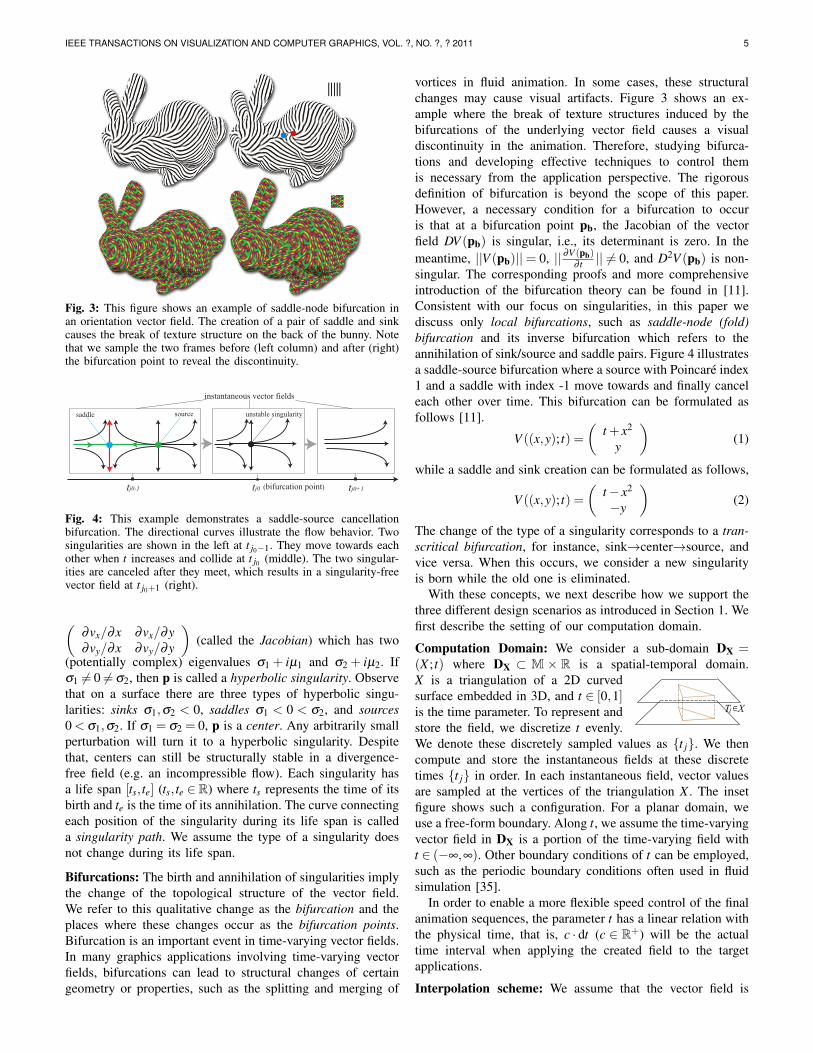
Fig. 3: This figure shows an example of saddle-node bifurcation inan orientation vector field. The creation of a pair of saddle and sinkcauses the break of texture structure on the back of the bunny. Notethat we sample the two frames before (left column) and after (right)the bifurcation point to reveal the discontinuity.

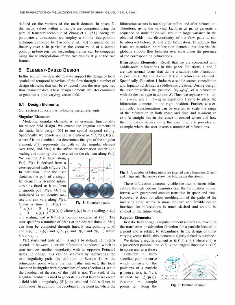
tj0-1 tj0 tj0+1

saddle source unstable singularity

(bifurcation point) �

instantaneous vector fields

Fig. 4: This example demonstrates a saddle-source cancellationbifurcation. The directional curves illustrate the flow behavior. Twosingularities are shown in the left at t j0−1. They move towards eachother when t increases and collide at t j0 (middle). The two singular-ities are canceled after they meet, which results in a singularity-freevector field at t j0+1 (right).

(∂vx/∂x ∂vx/∂y∂vy/∂x ∂vy/∂y

)(called the Jacobian) which has two

(potentially complex) eigenvalues σ1 + iµ1 and σ2 + iµ2. Ifσ1 6= 0 6= σ2, then p is called a hyperbolic singularity. Observethat on a surface there are three types of hyperbolic singu-larities: sinks σ1,σ2 < 0, saddles σ1 < 0 < σ2, and sources0 < σ1,σ2. If σ1 = σ2 = 0, p is a center. Any arbitrarily smallperturbation will turn it to a hyperbolic singularity. Despitethat, centers can still be structurally stable in a divergence-free field (e.g. an incompressible flow). Each singularity hasa life span [ts, te] (ts, te ∈R) where ts represents the time of itsbirth and te is the time of its annihilation. The curve connectingeach position of the singularity during its life span is calleda singularity path. We assume the type of a singularity doesnot change during its life span.

Bifurcations: The birth and annihilation of singularities implythe change of the topological structure of the vector field.We refer to this qualitative change as the bifurcation and theplaces where these changes occur as the bifurcation points.Bifurcation is an important event in time-varying vector fields.In many graphics applications involving time-varying vectorfields, bifurcations can lead to structural changes of certaingeometry or properties, such as the splitting and merging of

vortices in fluid animation. In some cases, these structuralchanges may cause visual artifacts. Figure 3 shows an ex-ample where the break of texture structures induced by thebifurcations of the underlying vector field causes a visualdiscontinuity in the animation. Therefore, studying bifurca-tions and developing effective techniques to control themis necessary from the application perspective. The rigorousdefinition of bifurcation is beyond the scope of this paper.However, a necessary condition for a bifurcation to occuris that at a bifurcation point pb, the Jacobian of the vectorfield DV (pb) is singular, i.e., its determinant is zero. In themeantime, ||V (pb)||= 0, || ∂V (pb)

∂ t || 6= 0, and D2V (pb) is non-singular. The corresponding proofs and more comprehensiveintroduction of the bifurcation theory can be found in [11].Consistent with our focus on singularities, in this paper wediscuss only local bifurcations, such as saddle-node (fold)bifurcation and its inverse bifurcation which refers to theannihilation of sink/source and saddle pairs. Figure 4 illustratesa saddle-source bifurcation where a source with Poincare index1 and a saddle with index -1 move towards and finally canceleach other over time. This bifurcation can be formulated asfollows [11].

V ((x,y); t) =(

t + x2

y

)(1)

while a saddle and sink creation can be formulated as follows,

V ((x,y); t) =(

t− x2

−y

)(2)

The change of the type of a singularity corresponds to a tran-scritical bifurcation, for instance, sink→center→source, andvice versa. When this occurs, we consider a new singularityis born while the old one is eliminated.

With these concepts, we next describe how we support thethree different design scenarios as introduced in Section 1. Wefirst describe the setting of our computation domain.

Computation Domain: We consider a sub-domain DX =(X ; t) where DX ⊂ M × R is a spatial-temporal domain.X is a triangulation of a 2D curvedsurface embedded in 3D, and t ∈ [0,1]is the time parameter. To represent andstore the field, we discretize t evenly.We denote these discretely sampled values as {t j}. We thencompute and store the instantaneous fields at these discretetimes {t j} in order. In each instantaneous field, vector valuesare sampled at the vertices of the triangulation X . The insetfigure shows such a configuration. For a planar domain, weuse a free-form boundary. Along t, we assume the time-varyingvector field in DX is a portion of the time-varying field witht ∈ (−∞,∞). Other boundary conditions of t can be employed,such as the periodic boundary conditions often used in fluidsimulation [35].

In order to enable a more flexible speed control of the finalanimation sequences, the parameter t has a linear relation withthe physical time, that is, c · dt (c ∈ R+) will be the actualtime interval when applying the created field to the targetapplications.

Interpolation scheme: We assume that the vector field is


defined on the vertices of the mesh domain. In space X ,the vector values within a triangle are computed using theparallel transport technique of Zhang et al. [51]. Along theparameter t dimension, we employ a similar interpolationtechnique proposed by Tricoche et al. [40] to guarantee thelinearity over t. In particular, the vector value of a samplepoint p in-between two succeeding frames can be computedusing linear interpolation of the two values at p at the twoframes.

5 ELEMENT-BASED DESIGNIn this section, we describe how we support the design of localspatial and temporal behaviors of the flow through a number ofdesign elements that can be extracted from the user-specifiedflow characteristics. These design elements are later combinedto generate a time-varying vector field.

5.1 Design ElementsOur system supports the following design elements.

Singular Elements:Modeling singular elements is an essential functionality

for vector field design. We extend the singular elements inthe static field design [51] to our spatial-temporal setting.Specifically, we denote a singular element as S(J,P(t),M(t)),where J is the Jacobian that determines the type of the singularelement, P(t) represents the path of the singular elementover time, and M(t) is the affine transformation matrix (i.e.scaling and rotating) that is exerted on the element along P(t).

Bi(x;t)=0�t0

(x0;t0)

y

x tj �tn�

(xj;tj)(xn;tn)

�0

�j�n

...... ......

t

y

x

Fig. 5: Singularity path.

We assume J is fixed alongP(t). P(t) is derived from auser-specified path (Figure 5).In particular, after the usersketches the path of a singu-lar element, a Hermite splinecurve is fitted to it to forma smooth path P(t). M(t) isinitialized as an identity ma-trix and can vary along P(t).Given a time tc, M(tc) =(

sx(tc) 00 sy(tc)

)R(θ(tc)) where sx(tc) is an x scaling, sy(tc)

a y scaling, and R(θ(tc)) a rotation centered at P(tc). Theuser specifies a number of M(ti) at the desired times ti. M(t)can then be computed through linearly interpolating sx(ti)and sx(ti+1), sy(ti) and sy(ti+1), and θ(ti) and θ(ti+1) whereti < t < ti+1.

P(t) starts and ends at t = 0 and 1 by default. If it startsor ends in between, a certain bifurcation is induced, which inturn involves another singularity with an opposite Poincareindex. In design, this can be achieved by intersecting thetwo singularity paths (by definition in Section 4). At thebifurcation point where the two paths intersect, the localJacobian is singular with eigenvalues of zero (Section 4), whilethe Jacobian of the rest of the field is not. That said, if thesingular Jacobian is used to generate a global field as we createa field with a singularity [51], the obtained field will not becontinuous. In addition, the Jacobian at the point pb where the

bifurcation occurs is not singular before and after bifurcation.Therefore, using the varying Jacobian at pb to generate asequence of static fields will result in large variance in theobtained fields, i.e., discontinuity of the flow patterns canbe observed before, at, and after bifurcation. To address thisissue, we introduce the bifurcation elements that describe theglobally smooth flow behavior over time under the presenceof the corresponding bifurcations.

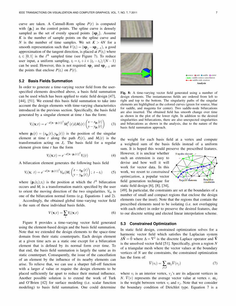
Bifurcation Elements: Recall that we are concerned withsaddle-node bifurcations in this paper. Equations 1 and 2are two normal forms that define a saddle-node bifurcationat position (0,0;0) in domain X (i.e. a bifurcation element).Specifically, Equation 1 induces a saddle-source cancellationand Equation 2 defines a saddle-sink creation. During design,the user prescribes the position, (x0,y0; t0), of a bifurcationwith the desired type in domain X . Thus, we replace x= x−x0,y = y− y0, and t = t − t0 in Equations 1 or 2 to place thebifurcation elements in the right position. Further, a user-controlled transformation can be exerted to scale the rangeof the bifurcation in both space and time and re-orient anaxis (a straight line in this case) to control where and howthe bifurcation occurs along the axis. Figure 6 provides anexample where the user inserts a number of bifurcations.

Fig. 6: A number of bifurcations are inserted using Equations 2 (red)and 1 (green). The arrows show the bifurcation directions.

These bifurcation elements enable the user to insert bifur-cations through certain templates (i.e. the bifurcation normalforms) with guaranteed smooth transition in space and time.However, it does not allow modification of the paths of theinvolving singularities. A more intuitive and flexible designinterface for bifurcations is much desired and should bestudied in the future work.

Regular Elements:In static field design, a regular element is useful in providing

the translation or advection direction for a particle located ata point and is related to streamlines. In the design of time-varying vector fields, this element is tightly linked to pathlines.

We define a regular element as R(V (t),P(t)) where P(t) isa prescribed pathline and V (t) is the tangent direction at P(t)in space and at a time t.

Fig. 7: Pathline example.

Consider a user-specified pathline curvewhich consists of thepositions of a particlep from ts to te (te ≥ ts),denoted by

⋃tts(p(s)).

Assume m samplepoints, pi, along the


curve are taken. A Catmull-Rom spline P(t) is computedwith {pi} as the control points. The spline curve is denselysampled as the set of evenly spaced points {sp j}. AssumeK is the number of sample points on the spline curve andN is the number of time samples. We set K > 4N for asmooth representation such that V (ti) = (sp j− sp j−1), a goodapproximation of the tangent direction, is placed at P(ti) whereti ∈ [0,1] is the ith sampled time (see Figure 7). To reduceuser input, a uniform sampling, ti = ts + i× (te− ts)/(N− 1)can be used. However, this is not required. sp j and sp j−1 arethe points that enclose P(ti) on P(t).

5.2 Basis Fields SummationIn order to generate a time-varying vector field from the user-specified elements described above, a basis field summationcan be used which has been applied to static field design [47],[44], [51]. We extend this basis field summation to take intoaccount the design elements with time-varying characteristicsintroduced in the previous section. Specifically, the basis fieldgenerated by a singular element at time t has the form:

Vi(x; t) = e−d‖x−pi(t)‖2MTi (t)JiMi(t)

(x− xpi(t)y− ypi(t)

)(3)

where pi(t) = (xpi(t),ypi(t)) is the position of the singularelement at time t along the path Pi(t), and Mi(t) is thetransformation acting on Ji. The basis field for a regularelement given time t has the form

Vi(x; t) = e−d‖x−pi(t)‖2Vi(t) (4)

A bifurcation element generates the following basis field

Vi(x; t) = e−d‖x−pi(t)‖2Vbi(Mi

(x− xpi(t)y− ypi(t)

); t− ti) (5)

where (pi(ti); ti) is the position at which the ith bifurcationoccurs and Mi is a transformation matrix specified by the userto orient the moving direction of the two singularities. Vbi isone of the bifurcation normal forms (e.g. Equations 1 and 2).

Accordingly, the obtained global time-varying vector fieldis the sum of these individual basis fields.

V (x; t) = ∑i

Vi(x; t) (6)

Figure 8 provides a time-varying vector field generatedusing the element-based design and the basis field summation.Note that we extended the design elements to the space-timedomain from their static counterparts. Each design elementat a given time acts as a static one except for a bifurcationelement that is defined by its normal form over time. Tothat end, the basis field summation is largely the same as itsstatic counterpart. Consequently, the issue of the cancellationof an element by the influence of its nearby elements canarise. To relieve that, we can use a sharper fall-off functionwith a larger d value or require the design elements to beplaced sufficiently far apart to reduce their mutual influence.Another possible solution is to extend the work of Turkand O’Brien [42] for surface modeling (i.e. scalar functionmodeling) to basis field summation. One could determine

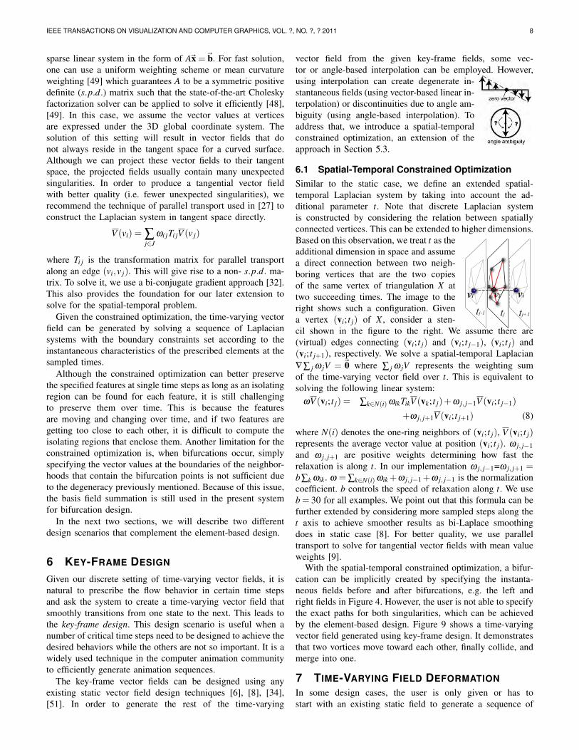
Fig. 8: A time-varying vector field generated using a number ofdesign elements. The instantaneous fields are ordered from left toright and top to the bottom. The singularity paths of the singularelements are highlighted as the colored curves (green for source, bluefor saddle, and magenta for center). Two saddle-node bifurcationsare also inserted. The obtained field has smooth change over timeas shown in the plot of the lower right. In addition to the desiredsingularities and bifurcations, there are also unexpected singularitiesand bifurcations as shown in the analysis, due to the nature of thebasis field summation approach.

the weight for each basis field at a vertex and computea weighted sum of the basis fields instead of a uniformsum. It is hoped this would preserve the prescribed features.However, it is unclear whethersuch an extension is easy todevise and how well it willwork for vector data. In thiswork, we resort to constrainedoptimization, a popular vectorfield generation technique forstatic field design [6], [8], [34],[49]. In particular, the constraints are set at the boundaries of anumber of small and compact regions that enclose the designelements (see the inset). Note that the regions that contain theprescribed elements need to be isolating (i.e. not overlappingwith each other) in order to preserve the desired features, dueto our discrete setting and elected linear interpolation scheme.

5.3 Constrained OptimizationIn static field design, constrained optimization solves for aharmonic vector field which satisfies the Laplacian system∆~V =~0 where ∆ = ∇2 is the discrete Laplace operator and ~Vis the unsolved vector field [51]. Specifically, given a region Nof a triangular mesh where the vector values at the boundaryvertices of N are the constraints, the constrained optimizationhas the form of:

V (vi) = ∑j∈J

ωi jV (v j) (7)

where vi is an interior vertex, v j’s are its adjacent vertices inN. V (v) represents the average vector value at vertex v. ωi jis the weight between vertex vi and v j. Note that we considerthe boundary condition of Dirichlet type. Equation 7 is a


sparse linear system in the form of A~x =~b. For fast solution,one can use a uniform weighting scheme or mean curvatureweighting [49] which guarantees A to be a symmetric positivedefinite (s.p.d.) matrix such that the state-of-the-art Choleskyfactorization solver can be applied to solve it efficiently [48],[49]. In this case, we assume the vector values at verticesare expressed under the 3D global coordinate system. Thesolution of this setting will result in vector fields that donot always reside in the tangent space for a curved surface.Although we can project these vector fields to their tangentspace, the projected fields usually contain many unexpectedsingularities. In order to produce a tangential vector fieldwith better quality (i.e. fewer unexpected singularities), werecommend the technique of parallel transport used in [27] toconstruct the Laplacian system in tangent space directly.

V (vi) = ∑j∈J

ωi jTi jV (v j)

where Ti j is the transformation matrix for parallel transportalong an edge (vi,v j). This will give rise to a non- s.p.d. ma-trix. To solve it, we use a bi-conjugate gradient approach [32].This also provides the foundation for our later extension tosolve for the spatial-temporal problem.

Given the constrained optimization, the time-varying vectorfield can be generated by solving a sequence of Laplaciansystems with the boundary constraints set according to theinstantaneous characteristics of the prescribed elements at thesampled times.

Although the constrained optimization can better preservethe specified features at single time steps as long as an isolatingregion can be found for each feature, it is still challengingto preserve them over time. This is because the featuresare moving and changing over time, and if two features aregetting too close to each other, it is difficult to compute theisolating regions that enclose them. Another limitation for theconstrained optimization is, when bifurcations occur, simplyspecifying the vector values at the boundaries of the neighbor-hoods that contain the bifurcation points is not sufficient dueto the degeneracy previously mentioned. Because of this issue,the basis field summation is still used in the present systemfor bifurcation design.

In the next two sections, we will describe two differentdesign scenarios that complement the element-based design.

6 KEY-FRAME DESIGN

Given our discrete setting of time-varying vector fields, it isnatural to prescribe the flow behavior in certain time stepsand ask the system to create a time-varying vector field thatsmoothly transitions from one state to the next. This leads tothe key-frame design. This design scenario is useful when anumber of critical time steps need to be designed to achieve thedesired behaviors while the others are not so important. It is awidely used technique in the computer animation communityto efficiently generate animation sequences.

The key-frame vector fields can be designed using anyexisting static vector field design techniques [6], [8], [34],[51]. In order to generate the rest of the time-varying

vector field from the given key-frame fields, some vec-tor or angle-based interpolation can be employed. However,using interpolation can create degenerate in-stantaneous fields (using vector-based linear in-terpolation) or discontinuities due to angle am-biguity (using angle-based interpolation). Toaddress that, we introduce a spatial-temporalconstrained optimization, an extension of theapproach in Section 5.3.

6.1 Spatial-Temporal Constrained OptimizationSimilar to the static case, we define an extended spatial-temporal Laplacian system by taking into account the ad-ditional parameter t. Note that discrete Laplacian systemis constructed by considering the relation between spatiallyconnected vertices. This can be extended to higher dimensions.

vivi vi

tjtj-1 tj+1

Based on this observation, we treat t as theadditional dimension in space and assumea direct connection between two neigh-boring vertices that are the two copiesof the same vertex of triangulation X attwo succeeding times. The image to theright shows such a configuration. Givena vertex (vi; t j) of X , consider a sten-cil shown in the figure to the right. We assume there are(virtual) edges connecting (vi; t j) and (vi; t j−1), (vi; t j) and(vi; t j+1), respectively. We solve a spatial-temporal Laplacian∇∑ j ω jV =~0 where ∑ j ω jV represents the weighting sumof the time-varying vector field over t. This is equivalent tosolving the following linear system:

ωV (vi; t j) = ∑k∈N(i) ωikTikV (vk; t j)+ω j, j−1V (vi; t j−1)

+ω j, j+1V (vi; t j+1) (8)

where N(i) denotes the one-ring neighbors of (vi; t j), V (vi; t j)represents the average vector value at position (vi; t j). ω j, j−1and ω j, j+1 are positive weights determining how fast therelaxation is along t. In our implementation ω j, j−1=ω j, j+1 =b∑k ωik. ω =∑k∈N(i) ωik+ω j, j−1+ω j, j−1 is the normalizationcoefficient. b controls the speed of relaxation along t. We useb = 30 for all examples. We point out that this formula can befurther extended by considering more sampled steps along thet axis to achieve smoother results as bi-Laplace smoothingdoes in static case [8]. For better quality, we use paralleltransport to solve for tangential vector fields with mean valueweights [9].

With the spatial-temporal constrained optimization, a bifur-cation can be implicitly created by specifying the instanta-neous fields before and after bifurcations, e.g. the left andright fields in Figure 4. However, the user is not able to specifythe exact paths for both singularities, which can be achievedby the element-based design. Figure 9 shows a time-varyingvector field generated using key-frame design. It demonstratesthat two vortices move toward each other, finally collide, andmerge into one.

7 TIME-VARYING FIELD DEFORMATIONIn some design cases, the user is only given or has tostart with an existing static field to generate a sequence of


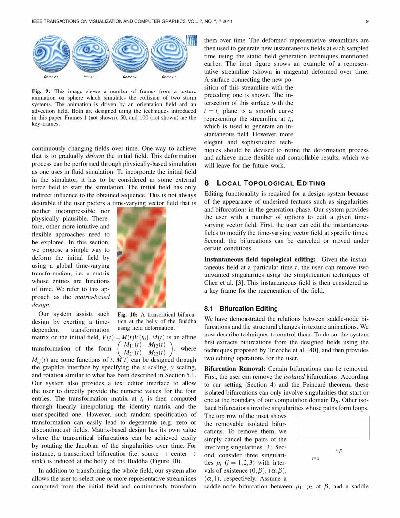
Fig. 9: This image shows a number of frames from a textureanimation on sphere which simulates the collision of two stormsystems. The animation is driven by an orientation field and anadvection field. Both are designed using the techniques introducedin this paper. Frames 1 (not shown), 50, and 100 (not shown) are thekey-frames.

continuously changing fields over time. One way to achievethat is to gradually deform the initial field. This deformationprocess can be performed through physically-based simulationas one uses in fluid simulation. To incorporate the initial fieldin the simulator, it has to be considered as some externalforce field to start the simulation. The initial field has onlyindirect influence to the obtained sequence. This is not alwaysdesirable if the user prefers a time-varying vector field that is

Fig. 10: A transcritical bifurca-tion at the belly of the Buddhausing field deformation.

neither incompressible norphysically plausible. There-fore, other more intuitive andflexible approaches need tobe explored. In this section,we propose a simple way todeform the initial field byusing a global time-varyingtransformation, i.e. a matrixwhose entries are functionsof time. We refer to this ap-proach as the matrix-baseddesign.

Our system assists suchdesign by exerting a time-dependent transformationmatrix on the initial field, V (t) = M(t)V (t0). M(t) is an affine

transformation of the form(

M11(t) M12(t)M21(t) M22(t)

), where

Mi j(t) are some functions of t. M(t) can be designed throughthe graphics interface by specifying the x scaling, y scaling,and rotation similar to what has been described in Section 5.1.Our system also provides a text editor interface to allowthe user to directly provide the numeric values for the fourentries. The transformation matrix at ti is then computedthrough linearly interpolating the identity matrix and theuser-specified one. However, such random specification oftransformation can easily lead to degenerate (e.g. zero ordiscontinuous) fields. Matrix-based design has its own valuewhere the transcritical bifurcations can be achieved easilyby rotating the Jacobian of the singularities over time. Forinstance, a transcritical bifurcation (i.e. source → center →sink) is induced at the belly of the Buddha (Figure 10).

In addition to transforming the whole field, our system alsoallows the user to select one or more representative streamlinescomputed from the initial field and continuously transform

them over time. The deformed representative streamlines arethen used to generate new instantaneous fields at each sampledtime using the static field generation techniques mentionedearlier. The inset figure shows an example of a represen-tative streamline (shown in magenta) deformed over time.A surface connecting the new po-sition of this streamline with thepreceding one is shown. The in-tersection of this surface with thet = ti plane is a smooth curverepresenting the streamline at ti,which is used to generate an in-stantaneous field. However, moreelegant and sophisticated tech-niques should be devised to refine the deformation processand achieve more flexible and controllable results, which wewill leave for the future work.

8 LOCAL TOPOLOGICAL EDITING

Editing functionality is required for a design system becauseof the appearance of undesired features such as singularitiesand bifurcations in the generation phase. Our system providesthe user with a number of options to edit a given time-varying vector field. First, the user can edit the instantaneousfields to modify the time-varying vector field at specific times.Second, the bifurcations can be canceled or moved undercertain conditions.

Instantaneous field topological editing: Given the instan-taneous field at a particular time t, the user can remove twounwanted singularities using the simplification techniques ofChen et al. [3]. This instantaneous field is then considered asa key frame for the regeneration of the field.

8.1 Bifurcation EditingWe have demonstrated the relations between saddle-node bi-furcations and the structural changes in texture animations. Wenow describe techniques to control them. To do so, the systemfirst extracts bifurcations from the designed fields using thetechniques proposed by Tricoche et al. [40], and then providestwo editing operations for the user.

Bifurcation Removal: Certain bifurcations can be removed.First, the user can remove the isolated bifurcations. Accordingto our setting (Section 4) and the Poincare theorem, theseisolated bifurcations can only involve singularities that start orend at the boundary of our computation domain DX. Other iso-lated bifurcations involve singularities whose paths form loops.The top row of the inset showsthe removable isolated bifur-cations. To remove them, wesimply cancel the pairs of theinvolving singularities [3]. Sec-ond, consider three singulari-ties pi (i = 1,2,3) with inter-vals of existence (0,β ), (α,β ),(α,1), respectively. Assume asaddle-node bifurcation between p1, p2 at β , and a saddle


node bifurcation between p2 and p3 at α . We then can removeboth bifurcations and retain only one singularity. The bottomrow of the inset shows such an example. The two bifurcationsthat are connected by the blue curve (the path of a saddle)can be collapsed. Figure 11 shows an example of saddle-nodebifurcation removal. More complex control of non-isolated(i.e. connected) bifurcations is possible, which is beyond thescope of this paper.

Fig. 11: Example of bifurcation editing.

Bifurcation Movement: Similar to singularities, a bifurcationcan be moved using our system. This can be achieved bymoving the involving singularities over space at particular timet. The edited instantaneous field is then set as a key frame.The spatial-temporal constrained optimization will smooththe rest of the field. Note that the movement of these twosingularities should obey the topological constraints proposedby Zhang et al. [51]. This guarantees that no other topologicalfeatures are affected during the movement. This functionalityis particularly useful when the bifurcation is not isolated andcauses visual discontinuity (e.g. Figure 3). The bifurcationmovement could move it to a non-visible part of the object.

General global smoothing over the spatial-temporal domainis also available, similar to the smoothing scheme of [18] forfining the edge fields, i.e. some tensor fields, in the applicationof painterly rendering of videos.

9 APPLICATIONS AND DISCUSSION

In this section, we present a number of graphics applicationsthat can benefit from the time-varying vector fields generatedusing the proposed techniques.

Texture Synthesis and AnimationWe have applied the designed time-varying fields to create

a number of synthetic texture animations (Figures 3 and 9).Flow-guided texture synthesis and advection has been intro-duced to the visualization community for dense flow visu-alization by van Wijk [44], [43], Laramee et al. [22], andNeyret [26]. Kwatra et al. [20] present an optimization-basedplane texture synthesis which can be used for flow-guidedtexture animation. Lefebvre and Hoppe [23] introduce anappearance-space texture synthesis technique that can handletexture advection over static surfaces. Han et al. [13] extendthe work of [20] to 3D mesh surfaces. Later, Kwatra etal. [19] and Bargteil et al. [2] extend the texture advectiontechniques to the problem of fluid texturing on surfaces.Recently, Ma et al. [24] introduce a texture synthesis techniquefor flow patterns to create a more detailed synthetic texture and

animation. In this paper, we employ the technique of Kwatraet al. [19]. To apply the created time-varying vector fields, wemake use of the instantaneous snapshots of the time-varyingvector fields to orient and move the texture patches on surfaces.

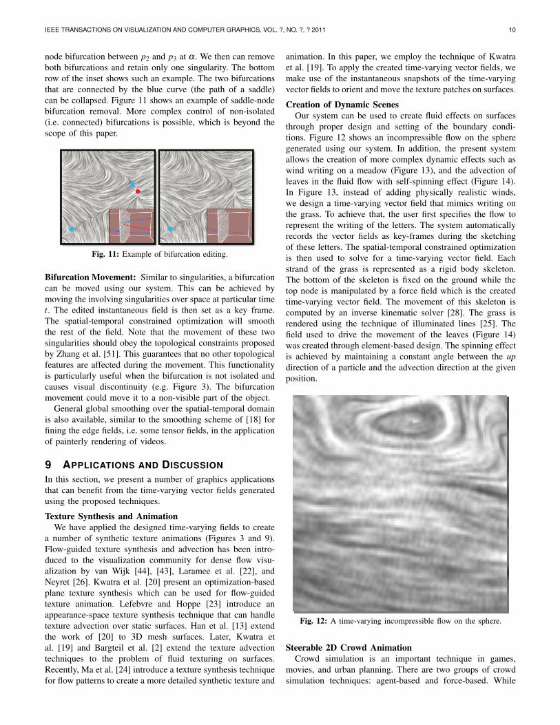
Creation of Dynamic ScenesOur system can be used to create fluid effects on surfaces

through proper design and setting of the boundary condi-tions. Figure 12 shows an incompressible flow on the spheregenerated using our system. In addition, the present systemallows the creation of more complex dynamic effects such aswind writing on a meadow (Figure 13), and the advection ofleaves in the fluid flow with self-spinning effect (Figure 14).In Figure 13, instead of adding physically realistic winds,we design a time-varying vector field that mimics writing onthe grass. To achieve that, the user first specifies the flow torepresent the writing of the letters. The system automaticallyrecords the vector fields as key-frames during the sketchingof these letters. The spatial-temporal constrained optimizationis then used to solve for a time-varying vector field. Eachstrand of the grass is represented as a rigid body skeleton.The bottom of the skeleton is fixed on the ground while thetop node is manipulated by a force field which is the createdtime-varying vector field. The movement of this skeleton iscomputed by an inverse kinematic solver [28]. The grass isrendered using the technique of illuminated lines [25]. Thefield used to drive the movement of the leaves (Figure 14)was created through element-based design. The spinning effectis achieved by maintaining a constant angle between the updirection of a particle and the advection direction at the givenposition.

Fig. 12: A time-varying incompressible flow on the sphere.

Steerable 2D Crowd AnimationCrowd simulation is an important technique in games,

movies, and urban planning. There are two groups of crowdsimulation techniques: agent-based and force-based. While


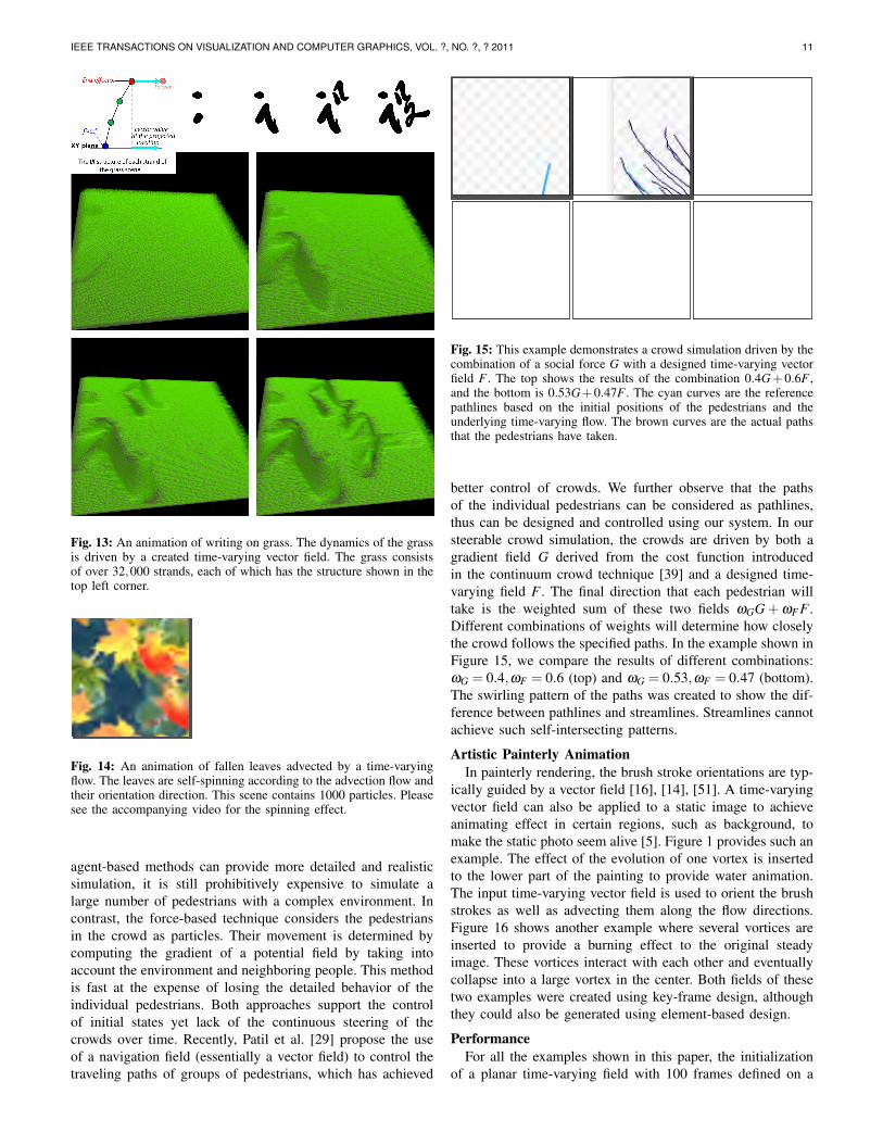
Fig. 13: An animation of writing on grass. The dynamics of the grassis driven by a created time-varying vector field. The grass consistsof over 32,000 strands, each of which has the structure shown in thetop left corner.

Fig. 14: An animation of fallen leaves advected by a time-varyingflow. The leaves are self-spinning according to the advection flow andtheir orientation direction. This scene contains 1000 particles. Pleasesee the accompanying video for the spinning effect.

agent-based methods can provide more detailed and realisticsimulation, it is still prohibitively expensive to simulate alarge number of pedestrians with a complex environment. Incontrast, the force-based technique considers the pedestriansin the crowd as particles. Their movement is determined bycomputing the gradient of a potential field by taking intoaccount the environment and neighboring people. This methodis fast at the expense of losing the detailed behavior of theindividual pedestrians. Both approaches support the controlof initial states yet lack of the continuous steering of thecrowds over time. Recently, Patil et al. [29] propose the useof a navigation field (essentially a vector field) to control thetraveling paths of groups of pedestrians, which has achieved

Fig. 15: This example demonstrates a crowd simulation driven by thecombination of a social force G with a designed time-varying vectorfield F . The top shows the results of the combination 0.4G+0.6F ,and the bottom is 0.53G+0.47F . The cyan curves are the referencepathlines based on the initial positions of the pedestrians and theunderlying time-varying flow. The brown curves are the actual pathsthat the pedestrians have taken.

better control of crowds. We further observe that the pathsof the individual pedestrians can be considered as pathlines,thus can be designed and controlled using our system. In oursteerable crowd simulation, the crowds are driven by both agradient field G derived from the cost function introducedin the continuum crowd technique [39] and a designed time-varying field F . The final direction that each pedestrian willtake is the weighted sum of these two fields ωGG + ωF F .Different combinations of weights will determine how closelythe crowd follows the specified paths. In the example shown inFigure 15, we compare the results of different combinations:ωG = 0.4,ωF = 0.6 (top) and ωG = 0.53,ωF = 0.47 (bottom).The swirling pattern of the paths was created to show the dif-ference between pathlines and streamlines. Streamlines cannotachieve such self-intersecting patterns.

Artistic Painterly AnimationIn painterly rendering, the brush stroke orientations are typ-

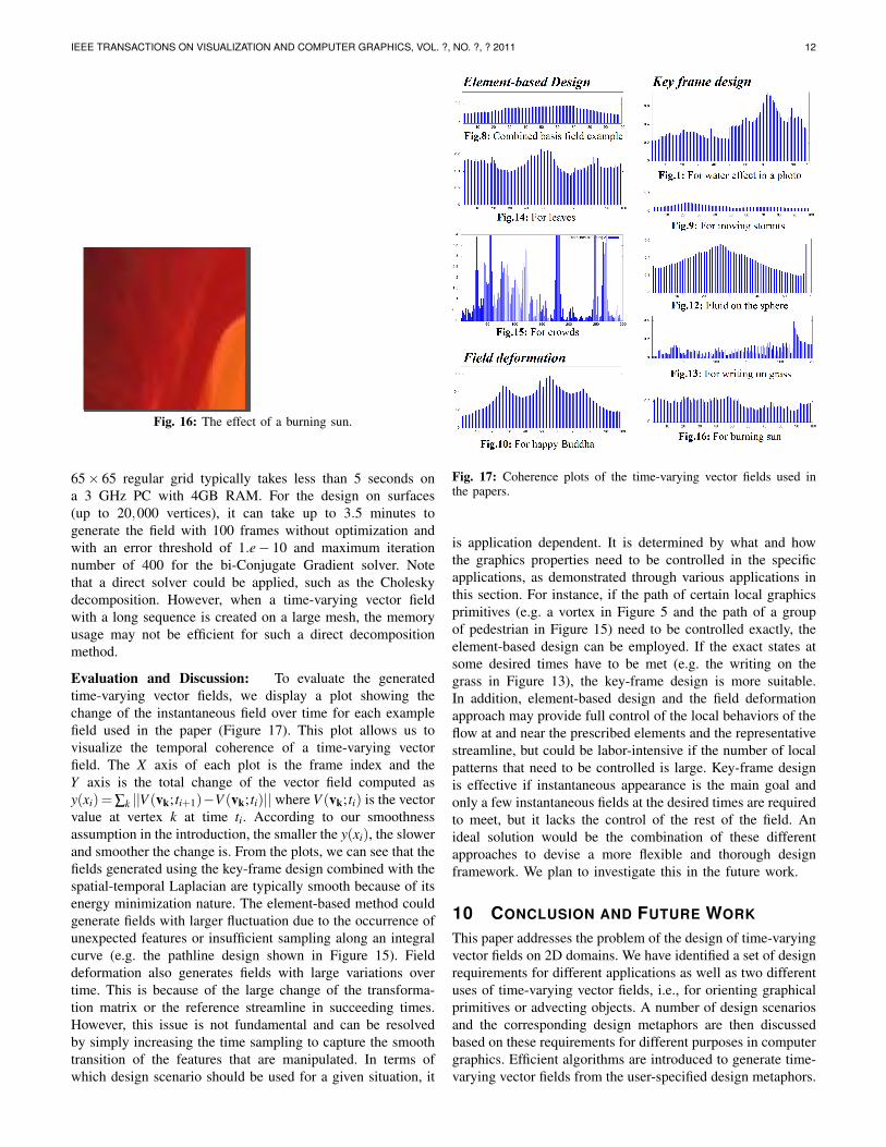
ically guided by a vector field [16], [14], [51]. A time-varyingvector field can also be applied to a static image to achieveanimating effect in certain regions, such as background, tomake the static photo seem alive [5]. Figure 1 provides such anexample. The effect of the evolution of one vortex is insertedto the lower part of the painting to provide water animation.The input time-varying vector field is used to orient the brushstrokes as well as advecting them along the flow directions.Figure 16 shows another example where several vortices areinserted to provide a burning effect to the original steadyimage. These vortices interact with each other and eventuallycollapse into a large vortex in the center. Both fields of thesetwo examples were created using key-frame design, althoughthey could also be generated using element-based design.

PerformanceFor all the examples shown in this paper, the initialization

of a planar time-varying field with 100 frames defined on a


Fig. 16: The effect of a burning sun.

65× 65 regular grid typically takes less than 5 seconds ona 3 GHz PC with 4GB RAM. For the design on surfaces(up to 20,000 vertices), it can take up to 3.5 minutes togenerate the field with 100 frames without optimization andwith an error threshold of 1.e− 10 and maximum iterationnumber of 400 for the bi-Conjugate Gradient solver. Notethat a direct solver could be applied, such as the Choleskydecomposition. However, when a time-varying vector fieldwith a long sequence is created on a large mesh, the memoryusage may not be efficient for such a direct decompositionmethod.

Evaluation and Discussion: To evaluate the generatedtime-varying vector fields, we display a plot showing thechange of the instantaneous field over time for each examplefield used in the paper (Figure 17). This plot allows us tovisualize the temporal coherence of a time-varying vectorfield. The X axis of each plot is the frame index and theY axis is the total change of the vector field computed asy(xi)=∑k ||V (vk; ti+1)−V (vk; ti)|| where V (vk; ti) is the vectorvalue at vertex k at time ti. According to our smoothnessassumption in the introduction, the smaller the y(xi), the slowerand smoother the change is. From the plots, we can see that thefields generated using the key-frame design combined with thespatial-temporal Laplacian are typically smooth because of itsenergy minimization nature. The element-based method couldgenerate fields with larger fluctuation due to the occurrence ofunexpected features or insufficient sampling along an integralcurve (e.g. the pathline design shown in Figure 15). Fielddeformation also generates fields with large variations overtime. This is because of the large change of the transforma-tion matrix or the reference streamline in succeeding times.However, this issue is not fundamental and can be resolvedby simply increasing the time sampling to capture the smoothtransition of the features that are manipulated. In terms ofwhich design scenario should be used for a given situation, it

Fig. 17: Coherence plots of the time-varying vector fields used inthe papers.

is application dependent. It is determined by what and howthe graphics properties need to be controlled in the specificapplications, as demonstrated through various applications inthis section. For instance, if the path of certain local graphicsprimitives (e.g. a vortex in Figure 5 and the path of a groupof pedestrian in Figure 15) need to be controlled exactly, theelement-based design can be employed. If the exact states atsome desired times have to be met (e.g. the writing on thegrass in Figure 13), the key-frame design is more suitable.In addition, element-based design and the field deformationapproach may provide full control of the local behaviors of theflow at and near the prescribed elements and the representativestreamline, but could be labor-intensive if the number of localpatterns that need to be controlled is large. Key-frame designis effective if instantaneous appearance is the main goal andonly a few instantaneous fields at the desired times are requiredto meet, but it lacks the control of the rest of the field. Anideal solution would be the combination of these differentapproaches to devise a more flexible and thorough designframework. We plan to investigate this in the future work.

10 CONCLUSION AND FUTURE WORK

This paper addresses the problem of the design of time-varyingvector fields on 2D domains. We have identified a set of designrequirements for different applications as well as two differentuses of time-varying vector fields, i.e., for orienting graphicalprimitives or advecting objects. A number of design scenariosand the corresponding design metaphors are then discussedbased on these requirements for different purposes in computergraphics. Efficient algorithms are introduced to generate time-varying vector fields from the user-specified design metaphors.


A number of editing operations with certain topological guar-antees are introduced to enable the fine adjustment of theobtained fields. We have incorporated the present techniquesinto a design system for the modeling of various time-varyingvector fields. To our knowledge, the presented design system isthe first of its kind for general time-varying vector field designwith bifurcation control. This work opens a new direction inthe area of field design which can be extended to the morecomplex time-varying field design problems. For instance, thesame framework can be easily modified to handle the designof time-varying tensor fields by extending the time-varyingsingular elements to the elements for degenerate points inthe element-based design or solving a tensor-based spatial-temporal Laplacian in the key frame design.

There are a number of future research directions. First, thepresent generation techniques do not guarantee the desiredtopology over time, especially for key frame design. Only thetopology at the key frame fields are defined. More comprehen-sive control of topology in between key frame fields is needed.Second, the bifurcation design is an important component intime-varying vector field design as shown in the paper. Moreflexible and sophisticated design techniques for bifurcationsare much desired. We also wish to extend our system to handlea variety of bifurcations that may involve more sophisticatedfeatures such as periodic orbits and separation and attach-ment lines. Third, we plan to explore other flow descriptorsincluding streaklines, timelines [7], and Lagrangian coherentstructures [12]. Fourth, more comprehensive combinationsof different design functionality and generation techniques,such as combining the presented design with physically-basedsimulation, should be studied to support more complex designtasks in the future. Finally, extending the design techniques for2D fields to 3D ones will be more challenging yet importantfor computer graphics.

ACKNOWLEDGMENTS

We would like to thank Dr. Konstantin Mischaikow for thevaluable discussion on the topology and dynamics of vectorfields, which initiated this work. We also thank Dr. Markvan Langeveld for the valuable discussion on potential ap-plications. We appreciate the help by Timothy O’Keefe onproofreading the paper. This work was supported by NSFIIS-0546881, IIS-0917308, OCI-0906379, and CCF-0830808award. Guoning Chen was partially supported by King Abdul-lah University of Science and Technology (KAUST) AwardNo. KUS-C1-016-04 and DOE VACET.

REFERENCES

[1] P. Alliez, D. Cohen-Steiner, O. Devillers, B. Levy, and M. Desbrun.Anisotropic polygonal remeshing. ACM Transactions on Graphics(SIGGRAPH 03), 22(3):485–493, 2003.

[2] A. W. Bargteil, F. Sin, J. E. Michaels, T. G. Goktekin, and J. F. O’Brien.A texture synthesis method for liquid animations. In SCA’06: Proceed-ings of the ACM SIGGRAPH/Eurographics Symposium on ComputerAnimation, pages 345–351, September 2006.

[3] G. Chen, K. Mischaikow, R. S. Laramee, P. Pilarczyk, and E. Zhang.Vector field editing and periodic orbit extraction using Morse decom-position. IEEE Transactions on Visualization and Computer Graphics,13(4):769–785, 2007.

[4] S. Chenney. Flow tiles. In SCA ’04: Proceedings of the 2004 ACMSIGGRAPH/Eurographics symposium on Computer animation, pages233–242. Eurographics Association, 2004.

[5] Y.-Y. Chuang, D. B. Goldman, K. C. Zheng, B. Curless, D. H. Salesin,and R. Szeliski. Animating pictures with stochastic motion textures.ACM Transactions on Graphics, 24(3):853–860, 2005.

[6] K. Crane, M. Desbrun, and P. Schroder. Trivial connections on discretesurfaces. Computer Graphics Forum (SGP), 29(5):1525–1533, 2010.

[7] T. Faber. Fluid Dynamics for Physicists. Cambridge University Press,1995.

[8] M. Fisher, P. Schroder, M. Desbrun, and H. Hoppe. Design of tangentvector fields. ACM Transactions on Graphics, 26(3):56:1–56:9, 2007.

[9] M. S. Floater. Mean value coordinates. Computer Aided GeometricDesign, 20(1):19–27, 2003.

[10] H. Fu, Y. Wei, C.-L. Tai, and L. Quan. Sketching hairstyles. In SBIM’07: Proceedings of the 4th Eurographics workshop on Sketch-basedinterfaces and modeling, pages 31–36. ACM, 2007.

[11] J. Hale and H. Kocak. Dynamics and Bifurcations. New York: Springer-Verlag, 1991.

[12] G. Haller. Finding finite-time invariant manifolds in two-dimensionalvelocity fields. Chaos, 10(1):99–108, 2000.

[13] J. Han, K. Zhou, L.-Y. Wei, M. Gong, H. Bao, X. Zhang, and B. Guo.Fast example-based surface texture synthesis via discrete optimization.The Visual Computer, 22(9):918–925, 2006.

[14] J. Hays and I. Essa. Image and video based painterly animation. InNPAR ’04: Proceedings of the 3rd international symposium on Non-photorealistic animation and rendering, pages 113–120, New York, NY,USA, 2004. ACM.

[15] J. L. Helman and L. Hesselink. Representation and display of vectorfield topology in fluid flow data sets. IEEE Computer, 22(8):27–36,1989.

[16] A. Hertzmann. Painterly rendering with curved brush strokes of multiplesizes. In Proceedings of the 25th annual conference on Computergraphics and interactive techniques, SIGGRAPH ’98, pages 453–460,New York, NY, USA, 1998. ACM.

[17] A. Hertzmann and K. Perlin. Painterly rendering for video and inter-action. In NPAR ’00: Proceedings of the 1st international symposiumon Non-photorealistic animation and rendering, pages 7–12, New York,NY, USA, 2000. ACM.

[18] M. Kagaya, W. Brendel, Q. Deng, T. Kesterson, S. Todorovic, P. J. Neill,and E. Zhang. Video painting with space-time-varying style parameters.IEEE Transactions on Visualization and Computer Graphics, 17(1):74–87, 2011.

[19] V. Kwatra, D. Adalsteinsson, T. Kim, N. Kwatra, M. Carlson, andM. Lin. Texturing fluids. IEEE Transactions on Visualization andComputer Graphics, 13(5):939–952, 2007.

[20] V. Kwatra, I. Essa, A. Bobick, and N. Kwatra. Texture optimization forexample-based synthesis. ACM Transactions on Graphics (SIGGRAPH05), 24:795–802, August 2005.

[21] Y.-K. Lai, M. Jin, X. Xie, Y. He, J. Palacios, E. Zhang, S.-M. Hu,and X. Gu. Metric-driven rosy field design and remeshing. IEEETransactions on Visualization and Computer Graphics, 16(1):95–108,2010.

[22] R. S. Laramee, B. Jobard, and H. Hauser. Image space based visualiza-tion of unsteady flow on surfaces. In Proceedings IEEE Visualization’03, pages 131–138. IEEE Computer Society, October 2003.

[23] S. Lefebvre and H. Hoppe. Appearance-space texture synthesis. ACMTransactions on Graphics (SIGGRAPH 06), 25(3):541–548, 2006.

[24] C. Ma, L.-Y. Wei, B. Guo, and K. Zhou. Motion field texture synthesis.ACM Transactions on Graphics, (SIGGRAPH Asia 2009), 28(5):110:1–110:8, 2009.

[25] O. Mallo, R. Peikert, C. Sigg, and F. Sadlo. Illuminated lines revisited.In Proceeding of IEEE Visualization 2005, pages 19–26, Los Alamitos,CA, USA, 2005. IEEE Computer Society.

[26] F. Neyret. Advected textures. In SCA ’03: Proceedings of the 2003ACM SIGGRAPH/Eurographics symposium on Computer animation,SCA ’03, pages 147–153, Aire-la-Ville, Switzerland, Switzerland, 2003.Eurographics Association.

[27] J. Palacios and E. Zhang. Rotational symmetry field design on surfaces.ACM Transactions on Graphics (SIGGRAPH 07), 26(3):56:1–56:10,2007.

[28] R. Parent. Computer Animation, Second Edition: Algorithms andTechniques. Morgan Kaufmann Publishers Inc., San Francisco, CA,USA, 2007.

[29] S. Patil, J. van den Berg, S. Curtis, M. C. Lin, and D. Manocha.Directing crowd simulations using navigation fields. IEEE Transactionson Visualization and Computer Graphics, 17(2):244–254, 2011.


[30] F. Pighin, J. M. Cohen, and M. Shah. Modeling and editing flows usingadvected radial basis functions. In SCA ’04: Proceedings of the 2004ACM SIGGRAPH/Eurographics symposium on Computer animation,pages 223–232. Eurographics Association, 2004.

[31] E. Praun, F. Adam, and H. Hugues. Lapped textures. In Proceedingsof the 27th annual conference on Computer graphics and interactivetechniques, SIGGRAPH ’00, pages 465–470, 2000.

[32] W. H. Press, S. A. Teukolsky, W. T. Vetterling, and B. P. Flannery.Numerical Recipes in C: The Art of Scientific Computing. New York,NY, USA: Cambridge University Press, 1992.

[33] N. Ray, W. C. Li, B. Lvy, and A. S. an d Pierre Alliez. Periodic globalparameterization. ACM Transactions on Graphics, 25(4):1460–1485,2006.

[34] N. Ray, B. Vallet, W.-C. Li, and B. Levy. N-symmetry direction fielddesign. ACM Transactions on Graphics, 27(2):10:1–10:13, 2008.

[35] J. Stam. Stable fluids. In Proceedings of the 26th annual conference onComputer graphics and interactive techniques, SIGGRAPH ’99, pages121–128. ACM Press/Addison-Wesley Publishing Co., 1999.

[36] J. Stam. Flows on surfaces of arbitrary topology. ACM Transactions onGraphics (SIGGRAPH 03), 22(3):724–731, July 2003.

[37] H. Theisel. Designing 2D vector fields of arbitrary topology. ComputerGraphics Forum (Eurographics 2002), 21(3):595–604, July 2002.

[38] H. Theisel, T. Weinkauf, H.-C. Hege, and H.-P. Seidel. Topologicalmethods for 2D time-dependent vector fields based on stream lines andpath lines. IEEE Transactions on Visualization and Computer Graphics,11(4):383–394, 2005.

[39] A. Treuille, S. Cooper, and Z. Popovic. Continuum crowds. ACMTransactions on Graphics (SIGGRAPH 06), 25(3):1160–1168, 2006.

[40] X. Tricoche, G. Scheuermann, and H. Hagen. Topology-based visu-alization of time-dependent 2D vector fields. In Data Visualization2001 (Joint Eurographics-IEEE TCVG Symposium on VisualizationProceedings), pages 117–126, 2001.

[41] G. Turk. Texture synthesis on surfaces. In Proceedings of the 28thannual conference on Computer graphics and interactive techniques,SIGGRAPH ’01, pages 347–354, 2001.

[42] G. Turk and J. F. O’brien. Modelling with implicit surfaces thatinterpolate. ACM Transactions on Graphics, 21(4):855–873, 2002.

[43] J. van Wijk. Image based flow visualization for curved surfaces. InProceedings IEEE Visualization ’03, pages 123–130. IEEE ComputerSociety, 2003.

[44] J. J. van Wijk. Image based flow visualization. ACM Transactions onGraphics (Siggraph 02), 21(3):745–754, July 2002.

[45] W. von Funck, H. Theisel, and H.-P. Seidel. Vector field based shapedeformations. ACM Transactions on Graphics, 25(3):1118–1125, 2006.

[46] L. Y. Wei and M. Levoy. Texture synthesis over arbitrary manifoldsurfaces. In Proceedings of the 28th annual conference on Computergraphics and interactive techniques, SIGGRAPH ’01, pages 355–360,2001.

[47] J. Wejchert and D. Haumann. Animation aerodynamics. In Proceedingsof the 18th annual conference on Computer graphics and interactivetechniques, SIGGRAPH ’91, pages 19–22. ACM, 1991.

[48] K. Xu, D. Cohne-Or, T. Ju, L. Liu, H. Zhang, S. Zhou, and Y. Xiong.Feature-aligned shape texturing. ACM Transactions on Graphics (SIG-GRAPH Asia 2009), 28(5):108:1–108:7, 2009.

[49] K. Xu, H. Zhang, D. Cohen-Or, and Y. Xiong. Dynamic harmonicfields for surface processing. Computers and Graphics (Shape ModelingInternational), 33(3):391–398, 2009.

[50] L. Xu, J. Chen, and J. Jia. A segmentation based variational modelfor accurate optical flow estimation. In ECCV ’08: Proceedings of the10th European Conference on Computer Vision: Part I, pages 671–684.Springer-Verlag, 2008.

[51] E. Zhang, K. Mischaikow, and G. Turk. Vector field design on surfaces.ACM Transactions on Graphics, 25(4):1294–1326, 2006.

Guoning Chen received a bachelors degree in1999 from Xi’an Jiaotong University, China and amasters degree in 2002 from Guangxi University,China. In 2009, he received a PhD degree incomputer science from Oregon State University.His research interests include scientific visual-ization, computational topology, and computergraphics. Currently, he is a post-doctoral re-search associate in Scientific Computing andImaging (SCI) Institute at the University of Utah.He is a member of the IEEE.

Vivek Kwatra Vivek Kwatra received the BTechdegree in computer science and engineeringfrom the Indian Institute of Technology (IIT)Delhi, India, in 1999 and the MS and PhD de-grees in computer science from the Georgia In-stitute of Technology in 2004 and 2005, respec-tively. He was a postdoctoral researcher in theComputer Science Department at the Universityof North Carolina, Chapel Hill, from 2005 to2007. He is currently working at Google as aresearch scientist.

Li-Yi Wei is an associate professor at The Uni-versity of Hong Kong. Before that he has beenwith Microsoft Research from 2005 to 2011 andNVIDIA from 2001 to 2005. He obtained Ph.D.from Stanford in 2001.

Charles D. Hansen received a BS in computerscience from Memphis State University in 1981and a PhD in computer science from the Univer-sity of Utah in 1987. He is a professor of com-puter science at the University of Utah an asso-ciate director of the SCI Institute. From 1989 to1997, he was a Technical Staff Member in theAdvanced Computing Laboratory (ACL) locatedat Los Alamos National Laboratory, where heformed and directed the visualization efforts inthe ACL. He was a Bourse de Chateaubriand

PostDoc Fellow at INRIA, Rocquencourt France, in 1987 and 1988.His research interests include large-scale scientific visualization andcomputer graphics.

Eugene Zhang received the PhD degree incomputer science in 2004 from Georgia Insti-tute of Technology. He is currently an associateprofessor at Oregon State University, where heis a member of the School of Electrical Engi-neering and Computer Science. His researchinterests include computer graphics, scientificvisualization, geometric modeling, and computa-tional topology. He received an National ScienceFoundation (NSF) CAREER award in 2006. Heis a senior member of the IEEE and a senior

member of ACM.

Documents

IEEE TRANSACTIONS ON VISUALIZATION AND ...chengu/Publications/TVCG11_timedep...IEEE TRANSACTIONS ON VISUALIZATION AND COMPUTER GRAPHICS, VOL., NO., ? 2011 1 Design of 2D Time-Varying