IEEE TRANSACTIONS ON PATTERN ANALYSIS AND · PDF fileIEEE TRANSACTIONS ON PATTERN ANALYSIS AND MACHINE INTELLIGENCE 1 Learning Multivariate Distributions by Competitive Assembly of

IEEE TRANSACTIONS ON PATTERN ANALYSIS AND MACHINE INTELLIGENCE 1

Learning Multivariate Distributionsby Competitive Assembly of Marginals

Francisco Sanchez-Vega, Jason Eisner, Laurent Younes, and Donald Geman.Johns Hopkins University, Baltimore, MD, USA

Abstract—We present a new framework for learning high-dimensional multivariate probability distributions from estimatedmarginals. The approach is motivated by compositional models and Bayesian networks, and designed to adapt to small samplesizes. We start with a large, overlapping set of elementary statistical building blocks, or “primitives”, which are low-dimensionalmarginal distributions learned from data. Each variable may appear in many primitives. Subsets of primitives are combined ina lego-like fashion to construct a probabilistic graphical model; only a small fraction of the primitives will participate in any validconstruction. Since primitives can be precomputed, parameter estimation and structure search are separated. Model complexityis controlled by strong biases; we adapt the primitives to the amount of training data and impose rules which restrict the mergingof them into allowable compositions. The likelihood of the data decomposes into a sum of local gains, one for each primitive in thefinal structure. We focus on a specific subclass of networks which are binary forests. Structure optimization corresponds to aninteger linear program and the maximizing composition can be computed for reasonably large numbers of variables. Performanceis evaluated using both synthetic data and real datasets from natural language processing and computational biology.

Index Terms—graphs and networks, statistical models, machine learning, linear programming

F

1 INTRODUCTION

P ROBABILISTIC graphical models provide a po-werful tool for discovering and representing the

statistical dependency structure of a family of randomvariables. Generally, these models exploit the dualitybetween conditional independence and separation ina graph in order to describe relatively complex jointdistributions using a relatively small number of para-meters. In particular, such graded models are poten-tially well-adapted to small-sample learning, wherethe bias-variance trade-off makes it necessary to investin model parameters with the utmost care. Learningmodels with a very reduced number of samples isno more difficult than with a great many. However,arranging for such models to generalize well to un-seen sets of observations, i.e., preventing them fromoverfitting the training data, remains an open andactive area of research in the small-sample domain.

The introduction of carefully chosen topologicalbiases, ideally consistent with prior domain know-ledge, can help to guide learning and avoid modeloverfitting. In practice, this can be accomplished byaccepting a restricted set of graph structures as well asby constraining the parameter space to only encode a

• F. Sanchez-Vega, L. Younes and D. Geman are with the Departmentof Applied Mathematics and Statistics, The Center for ImagingScience and the Institute for Computational Medicine, Johns HopkinsUniversity, 3400 N. Charles St., Baltimore, MD 21218. E-mail:sanchez, laurent.younes, [email protected].

• Jason Eisner is with the Department of Computer Science and theCenter for Language and Speech Processing, Johns Hopkins University,3400 N. Charles St., Baltimore, MD 21218. E-mail: [email protected]

restricted set of dependence statements. In either case,we are talking about the design of a model class inanticipation of efficient learning.

Our model-building strategy is “compositional” inthe sense of a lego-like assembly. We begin with a setof “primitives” — a large pool of low-dimensional,candidate distributions. Each variable may appear inmany primitives and only a small fraction of theprimitives will participate in any allowable construc-tion. A primitive designates some of its variables asinput (α variables) and others as output (ω variables).Primitives can be recursively merged into larger dis-tributions by matching inputs with outputs: in eachmerge, one primitive is designated the “connector”,and the other primitives’ α variables must match asubset of the connector’s ω variables. Matched vari-ables lose their α and ω designations in the result.The new distribution over the union of variables ismotivated by Bayesian networks, being the product ofthe connector’s distribution with the other primitives’distributions conditioned on their α nodes. In fact,each valid construction is uniquely identified with adirected acyclic graph over primitives.

The process is illustrated in Fig. 1 for a set offourteen simple primitives over twelve variables. Thisfigure shows an example of a valid construction withtwo connected components using six of the primitives.The form of the corresponding twelve-dimensionalprobability distribution will be explained in the text.Evidently, many other compositions are possible.

We seek the composition which maximizes the like-lihood of the data with respect to the empirical distri-bution over the training set. Due to the assembly pro-


Fig. 1. Simple example of primitives and assemblies.

cess, the global “score” (i.e., expected log-likelihood)of any valid composition decomposes into a sum oflocal scores, one for each participating primitive; thesescores are themselves likelihood ratios correspondingto the gain incurred in fusing the individual variablesinto the primitive distribution relative to indepen-dent variables. This decomposition has several con-sequences. First, all scores can be precomputed; con-sequently, parameter estimation (building primitives)and model construction (competitive assembly) areseparated. That is, once the primitives are learned theprocess is data-independent. Second, in many cases,searching over all decompositions for valid composi-tions can be done by integer linear programming.

The primary intended application is molecular net-work modeling in systems biology, where it is com-mon to encounter a complex underlying dependencystructure among a large number of variables and yeta very small number of samples, at least relative toother fields such as vision and language. DNA mi-croarrays provide simultaneous snap-shot measure-ments of the levels of expression of thousands ofgenes inside cells [1], [2], [3]. However, the number ofprofile measurements per experimental study remainsquite small, usually fewer than a few hundreds. Simi-larly, advances in genotyping microarrays currentlymake it possible to simultaneously detect single nu-cleotide polymorphisms (SNPs) over millions of locipractically covering the entire genome of an organism,while the number of individuals in any given studyremains orders of magnitude smaller [4], [5], [6].Thus, any attempt to infer generalizable multivariatedistributions from these data, in particular correla-tion patterns or even higher-dimensional interactions,must deal with well-known trade-offs in computa-tional learning theory between sample size and modelcomplexity [7], and between bias and variance [8].

Our proposals for model-building and complexitycontrol are illustrated with both synthetic and realdata. In the former case, experiments include measur-ing the KL divergence between the optimal composi-tion and the true distribution as a function of the sam-ple size and the number of variables. We compare ourgraphs with several well-known methods for “reverse

engineering” networks, including relevance networks[9], ARACNE [10], CLR [11], which infer graphs fromdata, and the K2 algorithm [12] for learning Bayesiannetworks. We present two real-data experiments. Oneis based on inferring a semantic network from text.The other involves learning dependencies among mu-tations of the gene TP53, which plays a central rolein cancer genomics. The substructures in the opti-mal composition appear biologically reasonable inthe sense of aggregating driver mutations and beingsignificantly enriched for certain cell functions. Still,we view our main contribution as methodological,these experiments being largely illustrative.

After discussing related work in Section 2, we willpresent the general theoretical framework for ourmodels in Section 3, followed by specialization to aspecific subclass based on balanced binary trees. InSection 4, we will discuss the choice of a statisticallysignificant set of primitives. These primitives are com-bined to build the graph structure that maximizesthe empirical likelihood of the observed data undera given set of topological constraints. In Section 5we will show how the corresponding optimizationproblem can be dealt with using either greedy searchor a more efficient integer linear programming formu-lation. Section 6 discusses the relationship of the fore-going approach to maximum a posteriori estimation ofgraphical model structure and parameters. After this,Section 7 presents some results from synthetic datasimulations. In Section 8 we will look at further resultsobtained using the 20newsgroups public dataset andthe IARC TP53 Database. Finally, we will provide ageneral discussion and we will sketch some directionsfor future research.

2 RELATED WORKHistorically, the problem of finding an optimumapproximation to a discrete joint probability distribu-tion has been addressed in the literature during thelast half century [13]. A seminal paper published byChow and Liu in the late sixties already proposed theuse of information theoretic measures to assess thegoodness of the approximation and formulated thestructure search as an optimization problem over aweighted graph [14]. Improvements to the original al-gorithm [15] as well as extensions beyond the originalpairwise approach [16] have been proposed. Recently,the popularity of Bayesian networks combined withthe need to face small-sample scenarios have led toseveral works where structural biases are imposedupon the graphs used to approximate the target dis-tribution in order to facilitate learning. Bounded tree-width is an example of such structural constraints.Even though the initial motivation for this approachwas to allow for efficient inference [17], [18], [19], therehas been work on efficient structure learning [20] andwork that uses this kind of bias to avoid model over-fitting [21]. Other examples of structural bias aimed


at achieving better generalization properties are theuse of L1 regularization to keep the number of edgesin the network under control [22], and constraintsprovided by experts [23]. We will discuss in Section 6how our method is related to these prior approaches.

Compositional representations of entities as hierar-chies of elementary, reusable parts that are combinedto form a larger whole constitute an active topic ofresearch in computer vision. Such modeling frame-works are usually built upon a set of compositionrules, based on parts and combinations of parts, thatprogressively define the likelihood of images giventhe presence of an object at a given pose [24], [25].A very simple composition rule, based on each partvoting for the presence of a relevant object around itslocation, under the assumption of complex poses, hasbeen proposed in [26]. The hierarchical structures in-duced by this kind of aggregation procedures providea convenient tool for hardwiring high-level contextualconstraints into the models [27], [28], [29], [30].

Dependency networks, which were proposed in[31] as an alternative to standard Bayesian networks,also provide an interesting example of compositionalmodeling, since they are built by first learning a setof small graph substructures with their correspondinglocal conditional probabilities. These “parts” are latercombined to define a single joint distribution usingthe machinery of Gibbs sampling. In any case, the ideaof combining compositional modeling and Bayesiannetworks dates back to the nineties, with the multi-ply sectioned Bayesian networks (MSBNs) from [32]and the object-oriented Bayesian networks (OOBNs)from [33]. Both approaches, as our work, provideways to combine a number of elementary Bayesiannetworks in order to construct a larger model. Thefinal structure can be seen as a hypergraph wherehypernodes correspond to those elementary buildingblocks and hyperlinks are used to represent relationsof statistical dependence among them. Hyperlinks aretypically associated to so-called “interfaces” betweenthe blocks, which correspond to non-empty pairwiseintersections of some of their constituting elements.Even though the actual definition of interface mayvary, it usually involves a notion of d-separation ofnodes at both of its sides within the network. Later on,the use of a relational structure to guide the learningprocess [34] and the introduction of structured datatypes based on hierarchical aggregations [35] (antici-pated in [33]) led to novel families of models.

All of the above approaches must confront thestructure search problem. That is, given a criterionfor scoring graphical models of some kind over theobserved variables, how do we computationally findthe single highest-scoring graph, either exactly orapproximately? Structure search is itself an approxi-mation to Bayesian model averaging as in [36], butit is widely used because it has the computationaladvantage of being a combinatorial optimization pro-

blem. In the case of Bayesian networks, Spirtes etal. [37, chapter 5] give a good review of earliertechniques, while Jaakkola et al. [38] review morerecent alternatives including exact ones. Like manyof these techniques (but unlike the module networksearch procedure in [39]), ours can be regarded asfirst selecting and scoring a set of plausible buildingblocks and only then seeking the structure with thebest total score [23]. We formalize this latter search asa problem of integer linear programming (ILP), muchas in [38], even if our building blocks have, in general,more internal structure. However, in the particularcase that we will present in this paper, we searchover more restricted assemblies of building blocks,corresponding to trees (generalizing [14]) rather thanDAGs. Thus, our ILP formulation owes more to recentwork on finding optimal trees, e.g., non-projectivesyntax trees in computational linguistics [40].

3 COMPETITIVE ASSEMBLY OF MARGINALS

In this section, we formulate structure search as acombinatorial optimization problem — CompetitiveAssembly of Marginals (CAM) — that is separated fromparameter estimation. The family of models that wewill consider is partially motivated by this searchproblem. We also present a specific subclass of modelstructures based on balanced binary forests.

3.1 General ConstructionOur objective is to define a class of multivariatedistributions for a family of random variables X =(Xi, i ∈ D) for D = {1, . . . , d}, where Xi takes valuesin a finite set Λ. For simplicity, we will assume thatall the Xi have the same domain, although in practiceeach Xi could have a different domain Λi. We shallrefer to the elements of ΛD as configurations.

First we mention the possibility of global, structuralconstraints: for each S ⊂ D, we are given a class MS

of “admissible” probability distributions over the setof subconfigurations ΛS (or over S, with some abuse).Our construction below will impose MS as a cons-traint on all joint distributions that we build over S.To omit such constraint, one can let MS consist of allprobability distributions on S. Let M∗ =

∪S⊂DMS .

If π ∈ M∗, we will write J(π) for its support, i.e., theuniquely defined subset of D such that π ∈ MJ(π).

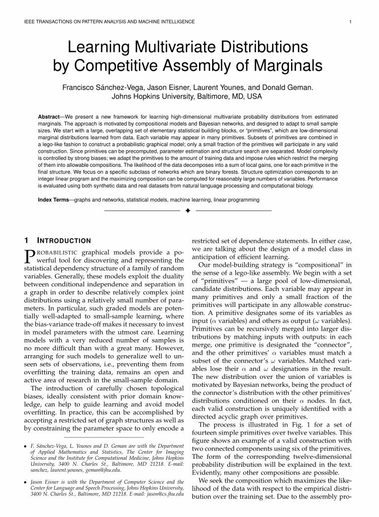
3.1.1 Primitives as Elementary Building BlocksThe main ingredient in our construction is a family T0of relatively simple probability distributions that wecall primitives. A distribution over X will be in ourclass only if it factors into a product of conditionaldistributions each of which is specified by a primitive.The elements of T0 are triplets ϕ = (π,A,O) whereπ ∈ M∗ and A,O are subsets of J(π) that serve as“connection nodes.” A set of five primitives is shownin Fig. 2. The variables (or “nodes”) in A will be called


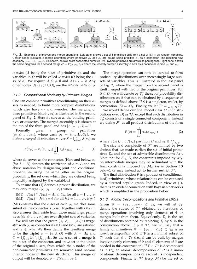
Fig. 2. Example of primitives and merge operations. Left panel shows a set of 5 primitives built from a set of |D| = 25 random variables.Center panel illustrates a merge operation where primitives ϕ1 and ϕ4 are bound using primitive ϕ3 as a connector. The resulting newassembly ϕ = Γ(ϕ3, ϕ1, ϕ4) is shown, as well as its associated primitive DAG (where primitives are drawn as pentagons). Right panel showsthe same diagrams for a second merge ϕ′ = Γ(ϕ, ϕ5, ϕ2) where the recently created assembly ϕ acts as a connector to bind ϕ5 and ϕ2.

α-nodes (A being the α-set of primitive ϕ), and thevariables in O will be called ω-nodes (O being the ω-set of ϕ). We require A,O = ∅ and A ∩ O = ∅. Anyother nodes, J(π) \ (A∪O), are the interior nodes of ϕ.

3.1.2 Compositional Modeling by Primitive Merges

One can combine primitives (conditioning on their α-sets as needed) to build more complex distributions,which also have α- and ω-nodes. The merging ofthree primitives (ϕ3, ϕ1, ϕ4) is illustrated in the secondpanel of Fig. 2. Here ϕ3 serves as the binding primi-tive, or connector. The merged assembly ϕ is shown atthe top of the third panel and has |A| = 1, |O| = 9.

Formally, given a group of primitives(ϕ0, ϕ1, . . . , ϕr), where each ϕk = (πk, Ak, Ok), wedefine a merged distribution π over S =

∪rk=0 J(πk) as:

π(xS) = π0(xJ(π0))r∏

k=1

πk(xJ(πk) | xAk) (1)

where ϕ0 serves as the connector. (Here and below, xI(for I ⊂ D) denotes the restriction of x to I , and weabuse notation by designating joint and conditionalprobabilities using the same letter as the originalprobability, the set over which they are defined beingimplicitly assigned by the variables.)

To ensure that (1) defines a proper distribution, wemay only merge (ϕ0, ϕ1, . . . , ϕr) when

(M1) J(πk)∩ J(π0) = Ak ⊂ O0, for all k = 1, . . . , r.(M2) J(πk) ∩ J(πl) = ∅ for all k, l = 1, . . . , r, k = l.

(M1) ensures that the α-set of each ϕk matches somesubset of the connector’s ω-set. Together with (M2), italso ensures that, aside from those matchings, primi-tives (ϕ0, ϕ1, . . . , ϕr) are over disjoint sets of variables.

We will say that the group (ϕ0, ϕ1, . . . , ϕr) is merge-able with ϕ0 as connector if (M1) and (M2) are satisfiedand π ∈ MS . We then define the resulting mergeto be the triplet ϕ = (π,A,O) with A = A0 andO =

∪rk=0Ok \

∪rk=1Ak. So the α-set of a merge is

the α-set of the connector, and its ω-set is the unionof the original ω-sets, from which the α-nodes of thenon-connector primitives are removed (and becomeinterior nodes in the new structure). This merge oroutput will be denoted ϕ = Γ(ϕ0, . . . , ϕr).

The merge operation can now be iterated to formprobability distributions over increasingly large sub-sets of variables. This is illustrated in the last panelof Fig. 2, where the merge from the second panel isitself merged with two of the original primitives. ForS ⊂ D, we will denote by T ∗

S the set of probability dis-tributions on S that can be obtained by a sequence ofmerges as defined above. If S is a singleton, we let, byconvention, T ∗

S = MS . Finally, we let T ∗ =∪S⊂D T ∗

S .We would define our final model class F∗ (of distri-

butions over D) as T ∗D, except that each distribution in

T ∗D consists of a single connected component. Instead

we define F∗ as all product distributions of the form

P (x) =

c∏k=1

πk(xJ(πk)) (2)

where J(π1), . . . , J(πc) partition D and πk ∈ T ∗J(πk)

.The size and complexity of F∗ are limited by two

choices that we made earlier: the set of initial primi-tives T0, and the set of admissible distributions M∗.Note that for S ( D, the constraints imposed by MS

on intermediate merges may be redundant with thefinal constraints imposed by MD (as in Section 3.3below), or may instead act to further restrict F∗.

The final distribution P is a product of (conditional-ized) primitives, whose relationships can be capturedby a directed acyclic graph. Indeed, in view of (1),there is an evident connection with Bayesian networkswhich is amplified in the proposition below.

3.1.3 Atomic Decompositions and Primitive DAGsGiven Ψ = {ψ1 . . . , ψN} ⊂ T0, we will let TΨdenote the subset of T ∗ obtained by iterations ofmerge operations involving only elements of Ψ ormerges built from them. Equivalently, TΨ is the setof distributions obtained by replacing T0 by Ψ in theconstruction above. If ϕ ∈ T ∗, we will say that afamily of primitives Ψ = {ψ1 . . . , ψN} ⊂ T0 is anatomic decomposition of ϕ if Ψ is a minimal subset ofT0 such that ϕ ∈ TΨ (i.e., ϕ can be built by mergesinvolving only elements of Ψ and all elements of Ψ areneeded in this construction). If P ∈ F∗ is decomposedas in (2), an atomic decomposition of P is a unionof atomic decompositions of each of its independentcomponents. Finally, let T ∗

0 (resp. F∗0 ) be the set of


atomic decompositions of elements of T ∗ (resp. F∗).The set of roots in the atomic decomposition Ψ ∈ T ∗

0

is denoted RΨ and defined as the set of indices k suchthat Ak ∩ J(πl) = ∅ for all k, l = 1, . . . , r, k = l.

Proposition 1. Let Ψ = {ψ1, . . . , ψN} ∈ T ∗0 with

ψk = (πk, Ak, Ok) and define the directed graph G(Ψ)on {1, . . . , N} by drawing an edge from k to l if and onlyif Al ⊂ Ok. Then G(Ψ) is acyclic.

This proposition is part of a larger one, PropositionS.1, which is stated and proved in Appendix I (seesupplemental material). The acyclic graph G(Ψ) isillustrated in Fig. 2 for the merges depicted in the mid-dle and right panels. Notice that the nodes of thesegraphs are primitives, not individual variables. Con-sequently, our models are Bayesian networks whosenodes are overlapping subsets of our variables X.

3.1.4 Generalization Using Weaker Merging RulesWe remark that the constraints defining merging rulescould be relaxed in several ways, resulting in lessrestricted model families. For example, one couldreplace (M2) by the weaker condition that supportsof non-connectors may intersect over their α-sets, i.e.,

(M2)’ J(πk) ∩ J(πl) ⊂ Ak ∩Al.Similarly, one can remove the constraint that ω-setsdo not intersect α-sets within a primitive, allowing formore flexible connection rules, as defined by (M1) (theω-set after merging would then simply be the unionof all previous ω-sets, without removing the α-sets).Such modifications do not affect the well-posednessof (1). An extreme case is when primitives contain allpossible pairs of variables, (M2) is replaced by (M2)’and the ω-set constraint is relaxed. Then our modelclass contains all possible Bayesian networks over thevariables (i.e., all probability distributions).

3.2 LikelihoodWe now switch to a statistical setting. We wish toapproximate a target probability distribution P ∗ onΛD by an element of F∗. This will be done by mini-mizing the Kullback-Leibler divergence between P ∗

and the model class. Equivalently, we maximize

L(P ) = EP∗(logP ) =∑x∈Λd

P ∗(x) logP (x), (3)

where P ∈ F∗. Typically, P ∗ is the empirical distribu-tion obtained from a training set, in which case theprocedure is just maximum likelihood.

Let each primitive distribution be parametric, ϕ =(π(·; θ), A,O), where θ is a parameter defined on a setΘϕ (which can depend on ϕ). From the definition ofmerge, it is convenient to restrict the distributions inF∗ by separately modeling the joint distribution ofthe α-nodes and the conditional distribution of theother nodes given the α-nodes. Therefore, we assumeθ = (σ, τ), where the restriction of π to A only depends

on σ and the conditional distribution on J(π)\A givenxA only depends on τ , i.e.,

π(xJ(π); θ) = π(xA;σ)π(xJ(π)\A | xA; τ).

We assume that single-variable distributions are un-constrained, i.e., there is a parameter Pj(λ) for eachλ ∈ Λ, j ∈ D.

In order to maximize L, we first restrict the pro-blem to distributions P ∈ F∗ which have an atomicdecomposition provided by a fixed family Ψ ={ψ1, . . . , ψN} ∈ F∗

0 . Afterwards, we will maximize theresult with respect to Ψ. Let θk = (σk, τk) ∈ Θψk

, k =1, . . . , N and let ℓ(θ1, ..., θN ) be the expected log-likelihood (3). Rewriting the maximum of ℓ based onlikelihood ratios offers an intuitive interpretation forthe “score” of each atomic decomposition in terms ofindividual likelihood gains relative to an independentmodel. For any primitive ϕ = (π(·; θ), A,O), define

ρ(ϕ) = maxθEP∗ log π(XJ(π); θ) (4)

−maxσ

EP∗ log π(XA;σ) +∑

j∈J(π)\A

H(P ∗j ),

where H(P ∗j ) = −EP∗

j(logP ∗

j ). This is the expectedlog-likelihood ratio of the estimated parametric modelfor Ψ and an estimated model in which i) all variablesin J \A are independent and independent from vari-ables in A, and ii) the model on A is the original one(parametrized with σ). We think of this as an internalbinding energy for primitive ϕ. Similarly, define

µ(ϕ) = maxσ

EP∗ log π(XA;σ) +∑j∈A

H(P ∗j ), (5)

the expected likelihood ratio between the (estimated)model on A and the (estimated) model which decou-ples all variables in A. Then it is rather straightfor-ward to show that the maximum log-likelihood ofany atomic decomposition decouples into primitive-specific terms. The proof, which resembles that of theChow-Liu theorem [14], is provided in Appendix II.

Proposition 2. Let ℓ(θ1, · · · , θN ) be the expectedlog-likelihood of the composition generated by Ψ =(ψ1, . . . , ψN ) ∈ F∗

0 . Then

maxθ1,...,θN

ℓ(θ1, · · · , θN ) = ℓ∗(Ψ)−∑j∈D

H(P ∗j )

where

ℓ∗(Ψ) =∑k∈RΨ

µ(ψk) +N∑k=1

ρ(ψk). (6)

Since the sum of entropies does not depend on Ψ,finding an optimal approximation of P ∗ “reduces”to maximizing ℓ∗ over all possible Ψ. More precisely,finding an optimal approximation requires computing

Ψ = argmaxΨ∈F∗

0

ℓ∗(Ψ) (7)

(with optimal parameters in (4) and (5)).


The important point is that the values of all ρ’sand µ’s can be precomputed for all primitives. Con-sequently, due to (6), any valid composition can bescored based only on the contributing primitives.In this way, parameter estimation is separated fromfinding the optimal Ψ. Obviously, the constraint Ψ ∈F∗

0 is far from trivial; it requires at least that Ψ satisfyconditions (i) and (ii) in Proposition S.1 (Appendix I).Moreover, computing Ψ typically involves a complexcombinatorial optimization problem. We will describeit in detail for the special case that is our focus.

3.3 Balanced Compositional Trees

We now specialize to a particular set of constraintsand primitives. In everything that follows, we willassume a binary state space, Λ = {0, 1}, and restrictthe admissible distributions M∗ to certain models thatcan be represented as trees (or forests), for whichwe introduce some notation. We call this subclass ofmodels balanced compositional trees.

If T is a tree, let J(T ) ⊂ D denote the set of nodesin T . For s ∈ J(T ), s+ denotes the set of children of sand s− the set of its parents. Because T is a tree, s−

has only one element, unless s is the root of the tree,in which case s− = ∅. We will say that T is binary ifno node has more than two children, i.e., |s+| ≤ 2 (weallow for nodes with a single child). If s+ = ∅ thens is called a terminal node, or leaf, and we let L(T )denote the set of all leaves in T . If s has two children,we will arbitrarily label them as left and right, withnotation s.l and s.r. Finally, Ts will denote the subtreeof T rooted at s, i.e., T restricted to the descendantsof s (including s). We will say that T is almost-balancedif for each s ∈ J(T ) such that |s+| = 2, the number ofleaves in Ts.l and Ts.r differ in at most one unit.

Probability distributions on ΛJ(T ) associated withT are assumed to be of the form:

π(xJ(T )) = p0(xs0)∏

s∈J(T )\L(T )

ps(xs+ | xs) (8)

where s0 is the root of T , p0 is a probability dis-tribution and ps, s ∈ J(T ) \ L(T ) are conditionaldistributions. This definition slightly differs from theusual one for tree models in that children do not haveto be conditionally independent given parents.

For S ⊂ D, we will let MS denote the set of modelsprovided by (8), in which T is an almost-balancedtree such that J(T ) = S. The balance constraint isintroduced as a desirable inductive bias intended tokeep the depth of the trees under control. The setT0 will consist of primitives ϕ = (π,A,O) where πis a probability distribution over a subset J ⊂ Dwith cardinality two or three; A (the α-set) is alwaysa singleton and we let O = J \ A. Primitives willbe selected based on training data, using a selectionprocess that will be described in the next section.

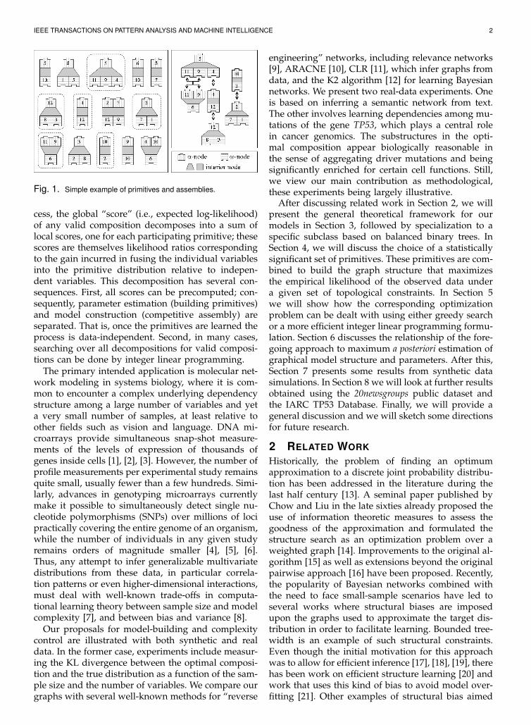
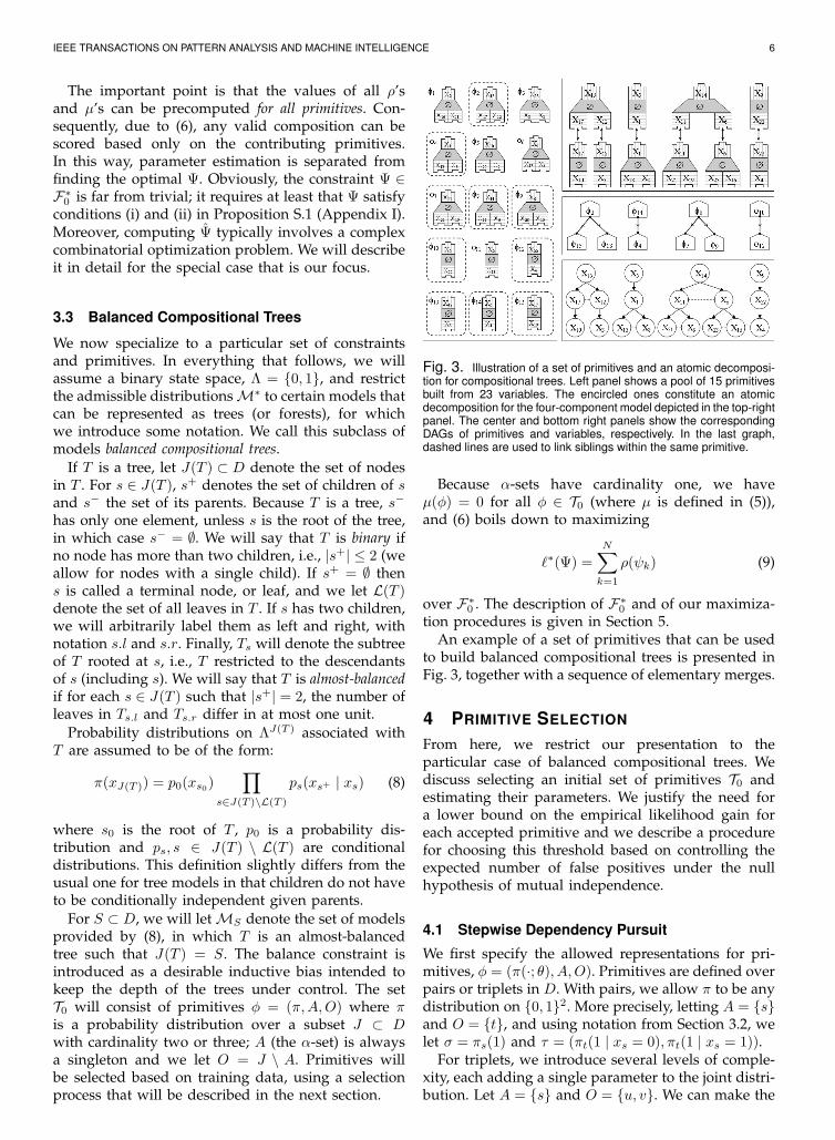
Fig. 3. Illustration of a set of primitives and an atomic decomposi-tion for compositional trees. Left panel shows a pool of 15 primitivesbuilt from 23 variables. The encircled ones constitute an atomicdecomposition for the four-component model depicted in the top-rightpanel. The center and bottom right panels show the correspondingDAGs of primitives and variables, respectively. In the last graph,dashed lines are used to link siblings within the same primitive.

Because α-sets have cardinality one, we haveµ(ϕ) = 0 for all ϕ ∈ T0 (where µ is defined in (5)),and (6) boils down to maximizing

ℓ∗(Ψ) =N∑k=1

ρ(ψk) (9)

over F∗0 . The description of F∗

0 and of our maximiza-tion procedures is given in Section 5.

An example of a set of primitives that can be usedto build balanced compositional trees is presented inFig. 3, together with a sequence of elementary merges.

4 PRIMITIVE SELECTION

From here, we restrict our presentation to theparticular case of balanced compositional trees. Wediscuss selecting an initial set of primitives T0 andestimating their parameters. We justify the need fora lower bound on the empirical likelihood gain foreach accepted primitive and we describe a procedurefor choosing this threshold based on controlling theexpected number of false positives under the nullhypothesis of mutual independence.

4.1 Stepwise Dependency Pursuit

We first specify the allowed representations for pri-mitives, ϕ = (π(·; θ), A,O). Primitives are defined overpairs or triplets in D. With pairs, we allow π to be anydistribution on {0, 1}2. More precisely, letting A = {s}and O = {t}, and using notation from Section 3.2, welet σ = πs(1) and τ = (πt(1 | xs = 0), πt(1 | xs = 1)).

For triplets, we introduce several levels of comple-xity, each adding a single parameter to the joint distri-bution. Let A = {s} and O = {u, v}. We can make the


joint distribution of (Xs, Xu, Xv) progressively moregeneral with the following steps:

(1) Xs, Xu, Xv are independent (3 parameters).(2) Xv⊥(Xs, Xu) (4 parameters).(2′) Xu⊥(Xs, Xv) (4 parameters).(3) Xu⊥Xv | Xs (5 parameters).(4) Xu⊥Xv | Xs = 0 (6 parameters).(4′) Xu⊥Xv | Xs = 1 (6 parameters).(5) Unconstrained joint (7 parameters).

Case (1) corresponds to the default singletons, and(2), (2’) involve a pair primitive and a singleton.“True” triplet distributions correspond to (3) through(5). The selection process that we now describe willassign one model to any selected triplet (s, u, v).

If d = |D| is the number of variables, there ared(d− 1) possible pairs and d(d− 1)(d− 2)/2 possibletriplets. Since we are targeting applications in which dcan reach hundreds or more, limiting the pool of pri-mitives is essential to limiting the complexity of bothstatistical estimation and combinatorial optimization.The selection will be based on a very simple principle:only accept a primitive at a given complexity levelwhen the previous level has been accepted and the ex-pected likelihood increment in passing to the higher-dimensional model is sufficiently large. So, whenbuilding a primitive ϕ = (π(·; θ), A,O) supported bya set J , with θ ∈ Θϕ, we will assume a sequence ofsubmodels Θ1 ⊂ Θ2 ⊂ · · · ⊂ Θq and let Θϕ be indexedby the largest k such that, for all l = 1, . . . , k − 1

maxθ∈Θl+1

EP∗ log π(XJ ; θ)−maxθ∈Θl

EP∗ log π(XJ ; θ) ≥ η

where η is a positive constant and P ∗ is the empiricaldistribution computed from observations. For exam-ple, to form a pair primitive over J = {u, v}, wecompare the joint empirical distribution over J (whichestimates three parameters) to the one for whichXu and Xv are independent (which estimates twoparameters), and we accept the pair primitive if

EP∗ logP ∗(Xu, Xv)

P ∗(Xu)P ∗(Xv)≥ η(2). (10)

(For simplicity, we are just writing P ∗(Xu, Xv) for theempirical joint distribution of Xu, Xv; in each casethe meaning should be clear from context.) In fact,we accept two primitives if this inequality is true:one for which u is the α-node and v the ω-node,and one for which the roles are reversed. Note thatselection for pairs reduces to applying a lower boundon the mutual information, the same selection rule asin relevance networks [9].

For triplets, we will apply the analysis to the se-quence of models (1), (2)/(2’), (3), . . . above. Forexample, to accept a triplet that corresponds to model(3), we first require that model (2) (or (2’)) is preferredto model (1), which implies that either the pair (s, u)or the pair (s, v) is accepted as a primitive using (10).

We then demand that model (3) is significantly betterthan, say, model (2), meaning that

EP∗ logP ∗(Xu | Xs)P

∗(Xv | Xs)

P ∗(Xu | Xs)P ∗(Xv)≥ η(3). (11)

To select model (4), we need model (3) to have beenselected first, and then, defining

P (xu, xv | xs) =

{P ∗(xu | xs)P ∗(xu | xs) if xs = 0

P ∗(xu, xv | xs) if xs = 1,

we will require

EP∗ logP (Xu, Xv | Xs)

P ∗(Xu | Xs)P ∗(Xv | Xs)≥ η(4). (12)

Selecting model (5) is done similarly, assuming thateither model (4) or (4)’ is selected.

4.2 Determination of the Selection ThresholdThe threshold η determines the number of selectedprimitives and will be based on an estimation of theexpected number of false detections. At each step ofthe primitive selection process, which correspond tothe five numbered steps from above, we will assumea null hypothesis consistent with the dependenciesaccepted up to the previous level and according towhich no new dependencies are added to the model.We will define η to ensure that the expected number ofdetections under this null is smaller than some ϵ > 0,which will be referred to as the selection threshold.

We will fix η(2) such that the expected number ofselected pairs under the assumption that all variablesare pairwise independent is smaller than ϵ. Assumingthat m(2) pairs have been selected, we will define η(3)to ensure that the expected number of selected tripletsof type (3) is smaller than ϵ, under the assumption thatany triplet of variables must be such that at least oneof the three is independent from the others. Similarly,assuming that m(3) triplets are selected, η(4) will bechosen to control the number of false alarms underthe hypothesis of all candidates following model (3).In some sense, selection at each level is done condi-tionally to the results obtained at the previous one.

At each step, the expected number of false alarmsfrom model (k − 1) to (k) can be estimated by ϵ,which is defined as the product of the number oftrials and the probability that model (k) is acceptedgiven that model (k − 1) is true. Since model (k) ispreferred to model (k − 1) when the likelihood ratiobetween the optimal models in each case is largerthan η(k), ϵ will depend on the distribution of thisratio when the smaller model is true. If the number ofobservations, n, is large enough, this distribution canbe estimated via Wilks’ theorem [41] which states thattwo times the likelihood ratio asymptotically followsa χ2 distribution, with degrees of freedom given bythe number of additional parameters (which is equalto one for each transition).


The number of trials for passing from level (3) to(4) and from level (4) to (5) is the number of selectedtriplets of the simplest type, i.e., t(3) = m(3) andt(4) = m(4) respectively. Between levels (2) and (3), wemake t(2) = (d−2)m(2) trials, and t(1) = d(d−1)/2 tri-als between levels (1) and (2). With this notation, andthe fact that each new level involves one additionalparameter, we use the following selection process: letη(k), k = 2, . . . , 5 be defined by

η(k) =1

2nF−1step

(1− ϵ

4t(k−1)

)(13)

where Fstep is the cumulative distribution function ofa χ2 with 1 d.f. (a standard normal squared) and thefactor 4 ensures that the total number of expected falsealarms across all levels is no more than ϵ.

For small values of n, the approximation based onWilks’ theorem is in principle not valid. Based onMonte-Carlo simulations, however, we observed thatit can be considered as reasonably accurate for n ≥ 20,which covers most practical cases. When n < 20,we propose to choose η(k) using Monte-Carlo (forvery large values of d, the number of required MonteCarlo replicates may become prohibitively large, butlearning distributions for extremely large d and n < 20may be a hopeless task to begin with).

5 STRUCTURE SEARCH ALGORITHM

The procedure defined in the previous section yieldsthe collection, T0, of building blocks that will be com-posed in the final model. Each of these blocks, say ψ,comes with their internal binding energy, ρ(ψ), whichcan be precomputed. The structure search problem, asdescribed in (9), consists in maximizing

ℓ∗(Ψ) =N∑k=1

ρ(ψk)

over all groups Ψ = {ψ1, . . . , ψN} ∈ F∗0 , i.e., all groups

of primitives that lead to a distribution on D that canbe obtained as a sequence of legal merges on Ψ.

We start by describing F∗0 . Recall that each family

Ψ = {ψ1, . . . , ψN} ⊂ T0 defines an oriented graphG(Ψ) on D, by inheriting the edges associated to eachof the ψk’s. We have the following fact (the proof isprovided in Appendix III, as supplemental material).

Proposition 3. A family of primitives Ψ ⊂ T0 belongs toF∗

0 if and only if(i) The α-nodes of the primitives are distinct.

(ii) The primitives do not share edges(iii) G(Ψ) is an almost-balanced binary forest.

These conditions can be checked without seeking aparticular sequence of admissible merges that yieldsG(Ψ). That is, the structure search problem reducesto maximizing ℓ∗(Ψ) over all Ψ = {ψ1, . . . , ψN}such that G(Ψ) is an almost-balanced forest. This is

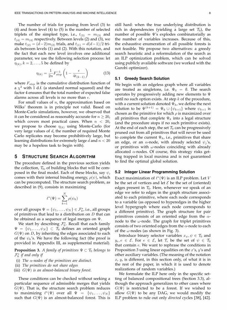
still hard: when the true underlying distribution isrich in dependencies (yielding a large set T0), thenumber of possible Ψ’s explodes combinatorially asthe number of variables increases. Because of this,the exhaustive enumeration of all possible forests isnot feasible. We propose two alternatives: a greedysearch heuristic and a reformulation of the search asan ILP optimization problem, which can be solvedusing publicly available software (we worked with theGurobi optimizer).

5.1 Greedy Search SolutionWe begin with an edgeless graph where all variablesare treated as singletons, i.e. Ψ0 = ∅. The searchoperates by progressively adding new elements to Ψuntil no such option exists. At step k of the procedure,with a current solution denoted Ψk, we define the nextsolution to be Ψ(k+1) = Ψk ∪ {ψk+1} where ψk+1 ischosen as the primitive for which ρ is maximized overall primitives that complete Ψk into a legal structure(and the procedure stops if no such primitive exists).At the end of each step, the set T0 can be progressivelypruned out from all primitives that will never be usedto complete the current Ψk, i.e., primitives that sharean edge, or an α-node, with already selected ψj ’s,or primitives with ω-nodes coinciding with alreadyallocated α-nodes. Of course, this strategy risks get-ting trapped in local maxima and is not guaranteedto find the optimal global solution.

5.2 Integer Linear Programming SolutionExact maximization of ℓ∗(Ψ) is an ILP problem. Let Vbe the set of vertices and let E be the set of (oriented)edges present in T0. Here, whenever we speak of anedge we refer to edges in the graph structure associ-ated to each primitive, where each node correspondsto a variable (as opposed to hyperedges in the higherlevel hypergraph where each node corresponds toa different primitive). The graph structure for pairprimitives consists of an oriented edge from the α-node to the ω-node. The graph for triplet primitivesconsists of two oriented edges from the α-node to eachof the ω-nodes (as shown in Fig. 3).

Introduce binary selector variables xψ, ψ ∈ T0 andye, e ∈ E . For e ∈ E , let Te be the set of ψ ∈ T0that contain e. We want to rephrase the conditions inProposition 3 using linear equalities on the x’s, y’s andother auxiliary variables. (The meaning of the notationx, y, is different, in this section only, of what it is inthe rest of the paper, in which it is used to denoterealizations of random variables.)

We formulate the ILP here only in the specific set-ting of balanced compositional trees (Section 3.3), al-though the approach generalizes to other cases whereG(Ψ) is restricted to be a forest. If we wished toallow G(Ψ) to be any DAG, we would modify theILP problem to rule out only directed cycles [38], [42].


The first constraint is, for all e ∈ E ,∑t∈Te

xt = ye,

which ensures that every selected edge belongs to oneand only one selected primitive.

We also need all edges in each selected primitive tobe accounted for, which gives, for all ψ ∈ T0,

(|ψ| − 1)xψ ≤∑e∈ψ

ye

where |ψ| is the number of vertices in ψ (two or three).For every directed edge e = (v, v′) with v, v′ ∈ V ,

let its reversal be e = (v′, v). Our next constraintimposes ye+ ye ≤ 1. Note that this constraint is maderedundant by the acyclicity constraint. Still, it may beuseful to speed up the solver.

Vertices must have no more than one parent and nomore than two children, which gives, for all v ∈ V ,∑

(v′,v)∈E

y(v′,v) ≤ 1 and∑

(v,v′)∈E

y(v,v′) ≤ 2.

We also ensure that no vertex is the α-node of twodistinct selected binary primitives. For v ∈ V , let Ψvdenote the subset of T0 containing binary primitiveswith {v} as an α-node. Then we want, for all v ∈ V∑

ψ∈Ψv

xψ ≤ 1.

The remaining conditions are more complex andrequire auxiliary variables. We first ensure that thegraph associated to the selected ψ’s is acyclic. Thiscan be done by introducing auxiliary flow variablesfe, e ∈ E with the constraint{−C(1− ye) + ye +

∑e′→e fe′ ≤ fe ≤ ye +

∑e′→e fe′

0 ≤ fe ≤ Cye

where C is large enough (e.g., C = |E|) and e′ →e means that the child in edge e′ coincides with theparent in edge e. (If ye = 1, this condition impliesfe = 1+

∑e′→e fe′ which is impossible unless fe = ∞

if the graph has a loop.)The last condition is for balance. Introduce variables

ge, e ∈ E and he, e ∈ E with constraints

0 ≤ he ≤ ye

he ≤ 1− ye′ if e→ e′

he ≥ 1−∑e→e′ ye′ − C(1− ye)

−C(1− ye) +∑e→e′ ge′ ≤ ge ≤ he +

∑e→e′ ge′

ye ≤ ge ≤ Cye

for all triplets ψ, |ge(ψ) − ge′(ψ)| ≤ 1 + C(1− xψ)

where e(ψ) and e′(ψ) denote the two edges in tripletψ. The variable he equals 1 if and only if e is a terminaledge. The variable ge counts the number of leaves (orterminal edges). We have ge = 0 if ye = 0. If e isterminal and ye = 1, then the sum over descendants

vanishes and the constraints imply ge = 1. Otherwise(he = 0 and ye = 1), we have ge =

∑e→e′ ge′ . The last

inequality ensures that the trees are almost-balanced.The original problem can now be solved by maxi-

mizing∑ψ∈T0

ρ(ψ)xψ subject to these constraints, theresulting solution being Ψ = {ψ : xψ = 1}.

ILP is a general language for formulating NP-complete problems. Although the worst-case runtimeof ILP solvers grows exponentially with the problemsize, some problem instances are much easier thanothers, and modern solvers are reasonably effective atsolving many practical instances of moderate size. Weshow empirical runtimes in Section II of the supple-mental material, together with an analysis of the sizeof the ILP encoding. Note that one can improve upongreedy search even without running the ILP solverto convergence, since the solver produces a series ofincreasingly good suboptimal solutions en route to theglobal optimum. Also, when the number of variablesand constraints in the ILP problem becomes compu-tationally prohibitive, we can adopt a hybrid searchstrategy: start by running a greedy search (whichtypically leads to a forest with several independentcomponents) and then solve multiple ILP problems asthe one described above, each restricted to ψ′s that aresupported by the set of variables involved in each ofthose components. Even though the solution may stillnot be globally optimal, this coarse-to-fine approachmay lead to improved performances over the use ofgreedy search and ILP alone.

6 CONNECTION WITH MAP LEARNING OFBAYESIAN NETWORK STRUCTURE

To situate our statistical approach with respect to theprior work of Section 2, we now discuss how it relatesto MAP estimation of Bayesian networks.

6.1 Primitives as Bayesian Networks

The approach that we propose in this paper consistsin constructing small-dimensional primitives, possiblyhaving complex parametrizations (if allowed by thedata-driven selection process), and assembling themglobally into a model covering all variables subjectto complexity contraints. Note that, even though theglobal relationship among primitives is organized as aBayesian network, as described in Section 3.1, the dis-tribution specified by each primitive can be modeledin an arbitrary way. We conceive of these primitivesas small modeling units, and the parametric repre-sentation introduced in Section 3.2 can be based onany appropriate model (one can use, for example, aMarkov random field built by progressive maximumentropy extension [43], selected similarly to Section 4).

In the case in which these primitives are alsomodeled as Bayesian networks, the global distributionof our model is obviously also represented as such.


This case includes the compositional trees introducedin Section 3.3, for which deriving a Bayesian networkrepresentation in cases (2)–(5) is straightforward.

In such a case, an alternative characterization ofour method is that we perform a structure searchover Bayesian networks that can be partitioned intopreviously selected primitives. In this regard, it canbe compared with other inductive biases, includingthe well-studied case of restricting the tree-widthof the graph, which leads to a maximum-likelihoodstructure search problem that is equivalent to findinga maximum-weight hyperforest [44], [45]. Our globalconstraints M∗ could be used to impose such a tree-width restriction on the graph over primitives, duringgreedy or global search. In particular, the composi-tional trees of Section 3.3 restrict this graph to tree-width 1, yielding our simpler combinatorial problemof finding a maximum-weight forest whose nodesare (possibly complex) primitives. Relaxing (M2) to(M2)’ in Section 3.1, we remark that if our primiti-ves consist of all Bayesian networks on subsets of≤ w + 1 variables, then assembling them under theglobal compositional-tree constraint gives a subset ofBayesian networks of tree-width w, while droppingthe global constraint gives the superset CPCPw [46].

6.2 Primitive Selection vs. MAP Estimation

Suppose we omit the initial step of primitive fil-tering. Then purely maximum-likelihood estimationcould be done using our global structure search algo-rithms from Section 5. Naturally, however, maximum-likelihood estimation will tend to overfit the data bychoosing models with many parameters. (Indeed, thisis the motivation for our approach.) A common rem-edy is instead to maximize some form of penalizedlog-likelihood. For many penalization techniques, thiscan be accomplished by the same global structuresearch algorithm over assemblies of primitives. Onemodifies the definition of each binding energy ρ(ψk)in our maximization objective (9) to add a constantpenalty that is more negative for more complex primi-tives ψk [23]. Before the search, it is safe to discard anyprimitive ψ such that the penalized binding energyρ(ψ) < ρ(ψ′) for some ψ′ with (J(ψ), A(ψ)), O(ψ)) =(J(ψ′), A(ψ′), O(ψ′)), since then ψ cannot appear inthe globally optimal structure [23]. The filtering stra-tegy in 4.1 can be regarded as a slightly more aggres-sive version of this, if the penalties are set to 0 fortriplets of type (1), −η(2) for those of type (2)/(2’),−(η(2) + η(3)) for those of type (3), and so on.

One can regard the total penalty of a structure asthe log of its prior probability (up to a constant).The resulting maximization problem can be seen asMAP estimation under a structural prior. To interpretour η penalties in this way would be to say that arandom model, a priori, is exp η(3) times less likely touse a given triplet of type (3) than one of type (2).

However, our actual approach differs from the aboveMAP story in two ways. First, it is not fully Bayesian,since in Section 4.2, we set the η parameters of theprior from our training data (cf. empirical Bayes orjackknifing). Second, a MAP estimator would includethe η penalties in the global optimization problem—but we use these penalties only for primitive selection.

Why the difference? While our approach is indeedsomewhat similar to MAP estimation with the aboveprior, that is not our motivation. We do not actuallysubscribe to a prior belief that simple structures aremore common than complex structures in our appli-cation domains (Section 8). Furthermore, our goal forstructure estimation is not to minimize the posteriorrisk under 0-1 loss, which is what MAP estimationdoes. Rather, we seek an estimator of structure thatbounds the risk of a model under a loss functiondefined as the number of locally useless correlationalparameters. Our structure selection procedure con-servatively enforces such a bound ϵ (by keeping thefalse discovery rate low even within T0 as a whole,and a fortiori within any model built from a subset ofT0). Subject to this procedure, we optimize likelihood,which minimizes the posterior risk under 0-1 loss fora uniform prior over structures and parameters.

We caution that ϵ does not bound the number ofincorrect edges relative to a true model. T0 includesall correlations that are valid within a primitive, evenif they would vanish when conditioning also on vari-ables outside the primitive (cf. [47]). To distinguishdirect from indirect correlations, our method usesonly global likelihood as in [14]. In the small-sampleregime, the resulting models (as with MAP) can havestructural errors but at least remain predictive withoutoverfitting—as we now show. Bounding the numberof incorrect edges would have to underfit, rejecting alledges, even if true or useful, that might be indirect.

7 SIMULATION STUDY

We assessed the performance of our learned modelsusing synthetic data. Here we present an overview ofour results. The full description of our simulations isprovided in Section I of the supplemental material.

We first run several experiments to measure theeffect of sample size, number of variables, selectionthreshold and search strategy upon learning perfor-mance when the true model belongs to our modelclass F∗. We evaluated the quality of the estimationby computing the KL divergence between the known,ground truth distribution and the distribution learnedusing our models. We evaluated network reconstruc-tion accuracy by building ROC and precision-recall(PR) curves in terms of true-positive and false-positiveedges. The actual curves and further details can befound in Section I.A of the supplemental material. Be-sides the obvious fact that both quality of estimationand network reconstruction accuracy improved with


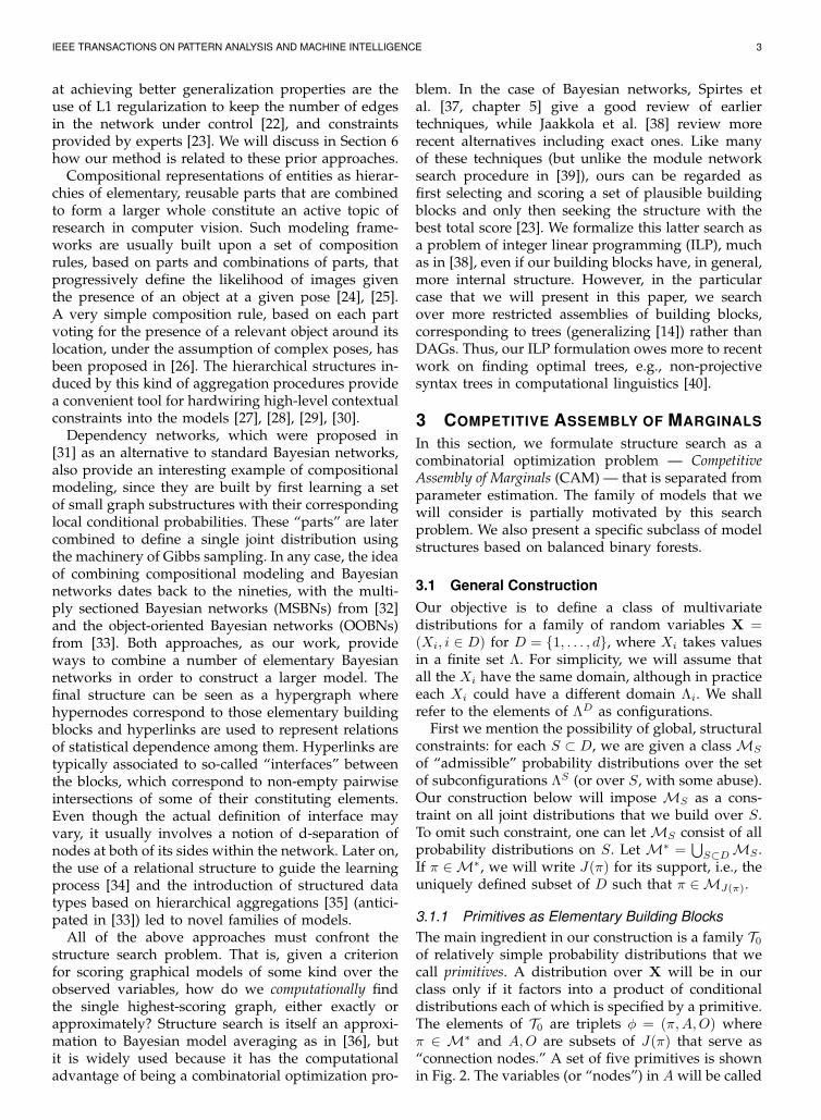
increasing sample sizes, our results showed that i) thechoice of an excessively large selection threshold leadsto model overfitting and ii) for very small samples,the distribution learned using CAM can be better (interms of KL divergence to the ground truth) thanthe distribution learned by using the true generatinggraph and estimating parameters from data.

20 40 60 80 100 120 140 160 180 2000

2

4

6

8

10

12

14

16

18

20

n

KL

200 400 600 800 1000 1200 1400 1600 1800 20000

0.1

0.2

0.3

0.4

0.5

0.6

0.7

0.8

n

KL

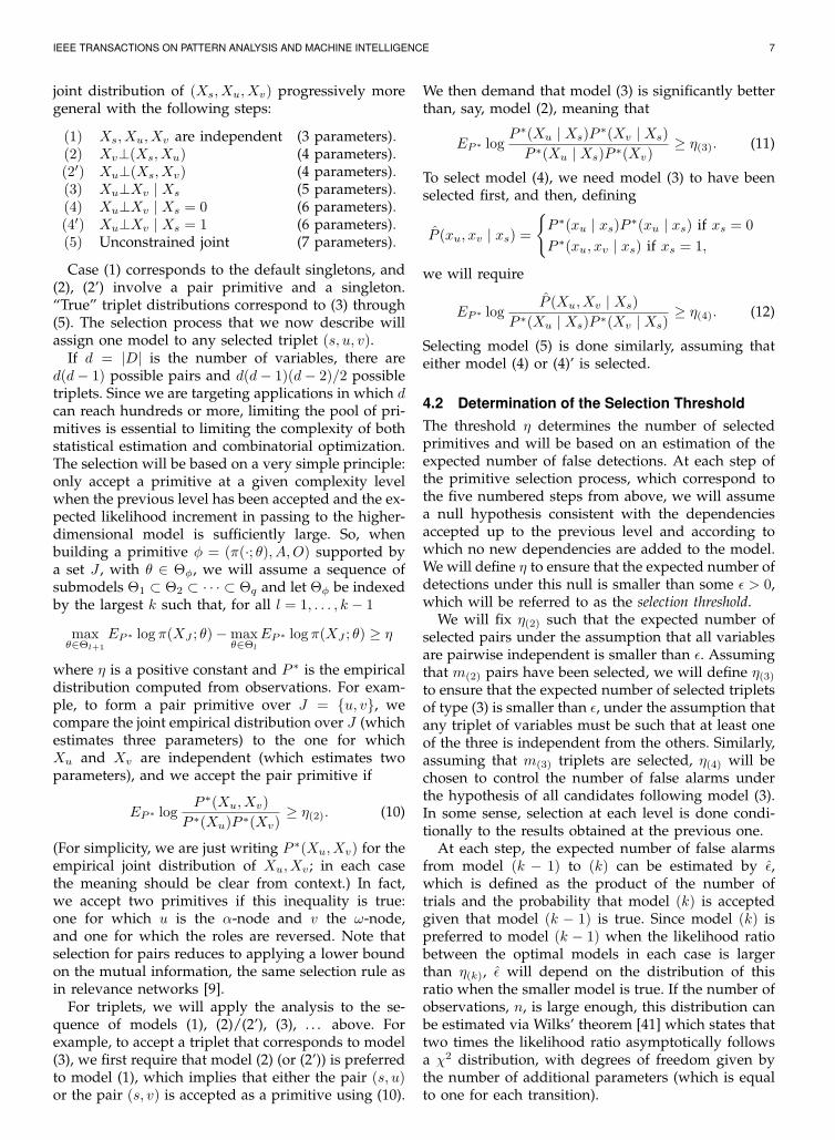
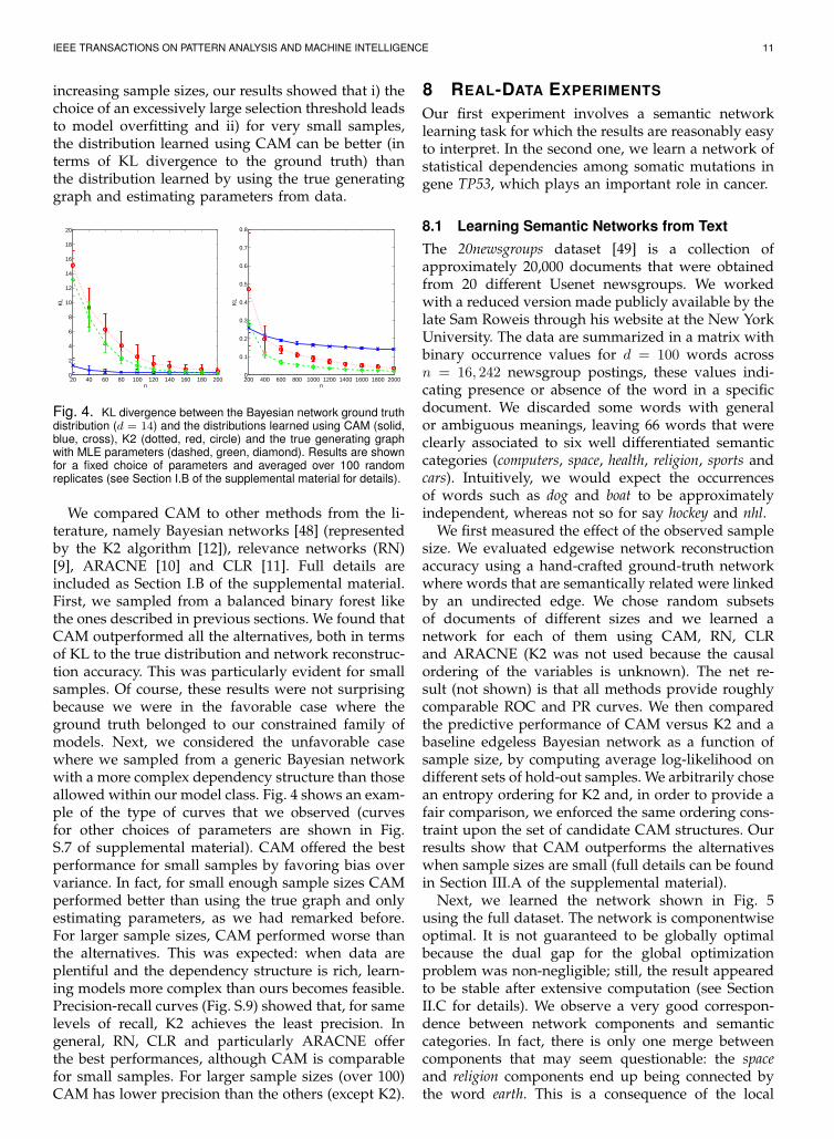
Fig. 4. KL divergence between the Bayesian network ground truthdistribution (d = 14) and the distributions learned using CAM (solid,blue, cross), K2 (dotted, red, circle) and the true generating graphwith MLE parameters (dashed, green, diamond). Results are shownfor a fixed choice of parameters and averaged over 100 randomreplicates (see Section I.B of the supplemental material for details).

We compared CAM to other methods from the li-terature, namely Bayesian networks [48] (representedby the K2 algorithm [12]), relevance networks (RN)[9], ARACNE [10] and CLR [11]. Full details areincluded as Section I.B of the supplemental material.First, we sampled from a balanced binary forest likethe ones described in previous sections. We found thatCAM outperformed all the alternatives, both in termsof KL to the true distribution and network reconstruc-tion accuracy. This was particularly evident for smallsamples. Of course, these results were not surprisingbecause we were in the favorable case where theground truth belonged to our constrained family ofmodels. Next, we considered the unfavorable casewhere we sampled from a generic Bayesian networkwith a more complex dependency structure than thoseallowed within our model class. Fig. 4 shows an exam-ple of the type of curves that we observed (curvesfor other choices of parameters are shown in Fig.S.7 of supplemental material). CAM offered the bestperformance for small samples by favoring bias overvariance. In fact, for small enough sample sizes CAMperformed better than using the true graph and onlyestimating parameters, as we had remarked before.For larger sample sizes, CAM performed worse thanthe alternatives. This was expected: when data areplentiful and the dependency structure is rich, learn-ing models more complex than ours becomes feasible.Precision-recall curves (Fig. S.9) showed that, for samelevels of recall, K2 achieves the least precision. Ingeneral, RN, CLR and particularly ARACNE offerthe best performances, although CAM is comparablefor small samples. For larger sample sizes (over 100)CAM has lower precision than the others (except K2).

8 REAL-DATA EXPERIMENTS

Our first experiment involves a semantic networklearning task for which the results are reasonably easyto interpret. In the second one, we learn a network ofstatistical dependencies among somatic mutations ingene TP53, which plays an important role in cancer.

8.1 Learning Semantic Networks from TextThe 20newsgroups dataset [49] is a collection ofapproximately 20,000 documents that were obtainedfrom 20 different Usenet newsgroups. We workedwith a reduced version made publicly available by thelate Sam Roweis through his website at the New YorkUniversity. The data are summarized in a matrix withbinary occurrence values for d = 100 words acrossn = 16, 242 newsgroup postings, these values indi-cating presence or absence of the word in a specificdocument. We discarded some words with generalor ambiguous meanings, leaving 66 words that wereclearly associated to six well differentiated semanticcategories (computers, space, health, religion, sports andcars). Intuitively, we would expect the occurrencesof words such as dog and boat to be approximatelyindependent, whereas not so for say hockey and nhl.

We first measured the effect of the observed samplesize. We evaluated edgewise network reconstructionaccuracy using a hand-crafted ground-truth networkwhere words that are semantically related were linkedby an undirected edge. We chose random subsetsof documents of different sizes and we learned anetwork for each of them using CAM, RN, CLRand ARACNE (K2 was not used because the causalordering of the variables is unknown). The net re-sult (not shown) is that all methods provide roughlycomparable ROC and PR curves. We then comparedthe predictive performance of CAM versus K2 and abaseline edgeless Bayesian network as a function ofsample size, by computing average log-likelihood ondifferent sets of hold-out samples. We arbitrarily chosean entropy ordering for K2 and, in order to provide afair comparison, we enforced the same ordering cons-traint upon the set of candidate CAM structures. Ourresults show that CAM outperforms the alternativeswhen sample sizes are small (full details can be foundin Section III.A of the supplemental material).

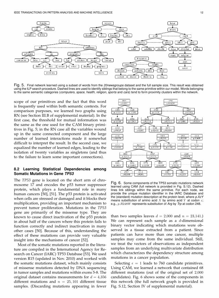
Next, we learned the network shown in Fig. 5using the full dataset. The network is componentwiseoptimal. It is not guaranteed to be globally optimalbecause the dual gap for the global optimizationproblem was non-negligible; still, the result appearedto be stable after extensive computation (see SectionII.C for details). We observe a very good correspon-dence between network components and semanticcategories. In fact, there is only one merge betweencomponents that may seem questionable: the spaceand religion components end up being connected bythe word earth. This is a consequence of the local


Fig. 5. Final network learned using a subset of words from the 20newsgroups dataset and the full sample size. This result was obtainedusing the ILP search procedure. Dashed lines are used to identify siblings that belong to the same primitive within our model. Words belongingto the same semantic categories (computers, space, health, religion, sports and cars) tend to form proximity clusters within the network.

scope of our primitives and the fact that this wordis frequently used within both semantic contexts. Forcomparison purposes, we learned two graphs usingRN (see Section III.B of supplemental material). In thefirst case, the threshold for mutual information wasthe same as the one used for the CAM binary primi-tives in Fig. 5; in the RN case all the variables woundup in the same connected component and the largenumber of learned interactions made it somewhatdifficult to interpret the result. In the second case, weequalized the number of learned edges, leading to theisolation of twenty variables as singletons (and thusto the failure to learn some important connections).

8.2 Learning Statistical Dependencies amongSomatic Mutations in Gene TP53

The TP53 gene is located on the short arm of chro-mosome 17 and encodes the p53 tumor suppressorprotein, which plays a fundamental role in manyhuman cancers [50], [51]. The p53 protein is activatedwhen cells are stressed or damaged and it blocks theirmultiplication, providing an important mechanism toprevent tumor proliferation. Mutations in the TP53gene are primarily of the missense type. They areknown to cause direct inactivation of the p53 proteinin about half of the cancers where this protein fails tofunction correctly and indirect inactivation in manyother cases [50]. Because of this, understanding theeffect of these mutations can provide very valuableinsight into the mechanisms of cancer [52].

Most of the somatic mutations reported in the litera-ture are compiled in the International Agency for Re-search on Cancer (IARC) TP53 Database [53]. We usedversion R15 (updated in Nov. 2010) and worked withthe somatic mutations dataset, which mainly consistsof missense mutations detected by DNA sequencingin tumor samples and mutations within exons 5-8. Theoriginal dataset contains measurements for d = 4,356different mutations and n = 25, 101 different tissuesamples. (Discarding mutations appearing in fewer

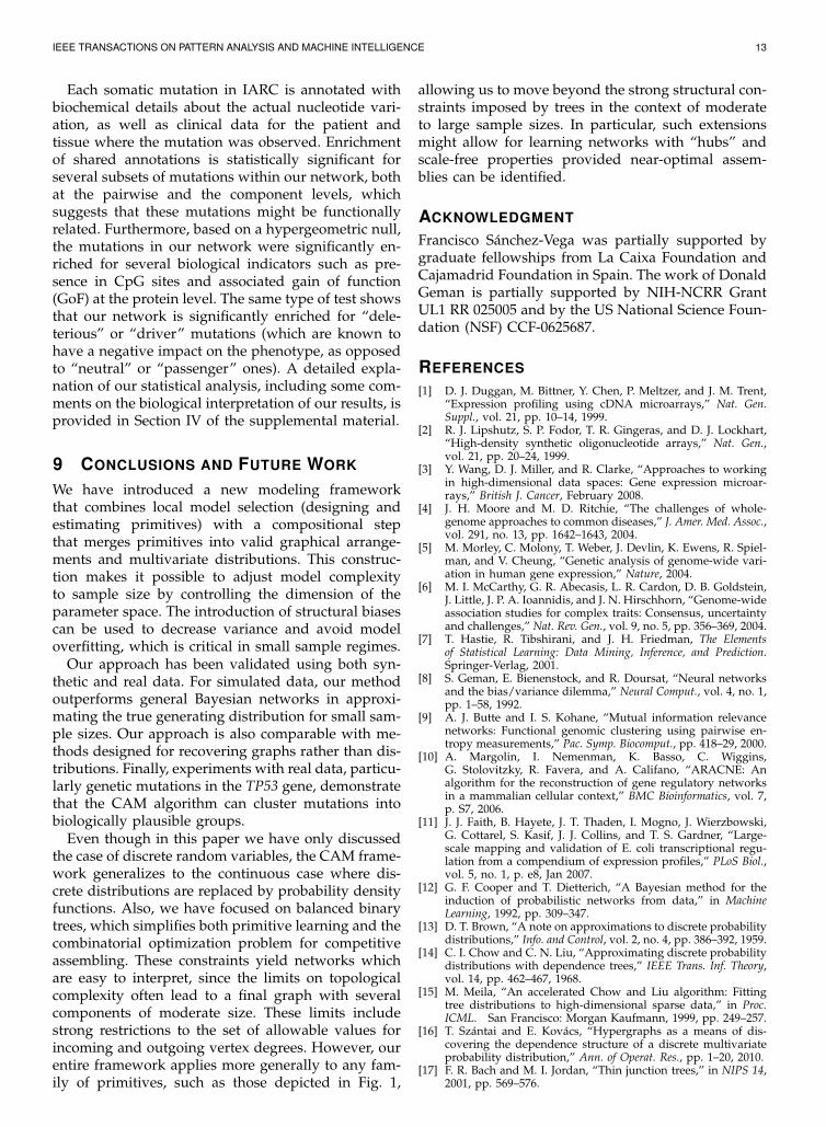
Fig. 6. Some components of the TP53 somatic mutations networklearned using CAM (full network is provided in Fig. S.12). Dashedlines link siblings within the same primitive. For each node, weprovide the unique mutation identifier in the IARC Database andthe (standard) mutation description at the protein level, where p.XzYmeans substitution of amino acid X by amino acid Y at codon z;e.g., p.R248W represents substitution of Arg by Trp at codon 248.

than two samples leaves d = 2,000 and n = 23,141.)We can represent each sample as a d-dimensionalbinary vector indicating which mutations were ob-served in a tissue extracted from a patient. Sincepatients can have more than one cancer, multiplesamples may come from the same individual. Still,we treat the vectors of observations as independentsamples from an underlying multivariate distributionwhich characterizes the dependency structure amongmutations in a cancer population.

Selecting ϵ = 1 leads to 760 candidate primitives.Using CAM, we learned a network that contained 68different mutations (out of the original set of 2,000candidates). Fig. 6 shows some of the components inthis network (the full network graph is provided inFig. S.12, Section IV of supplemental material).


Each somatic mutation in IARC is annotated withbiochemical details about the actual nucleotide vari-ation, as well as clinical data for the patient andtissue where the mutation was observed. Enrichmentof shared annotations is statistically significant forseveral subsets of mutations within our network, bothat the pairwise and the component levels, whichsuggests that these mutations might be functionallyrelated. Furthermore, based on a hypergeometric null,the mutations in our network were significantly en-riched for several biological indicators such as pre-sence in CpG sites and associated gain of function(GoF) at the protein level. The same type of test showsthat our network is significantly enriched for “dele-terious” or “driver” mutations (which are known tohave a negative impact on the phenotype, as opposedto “neutral” or “passenger” ones). A detailed expla-nation of our statistical analysis, including some com-ments on the biological interpretation of our results, isprovided in Section IV of the supplemental material.

9 CONCLUSIONS AND FUTURE WORK

We have introduced a new modeling frameworkthat combines local model selection (designing andestimating primitives) with a compositional stepthat merges primitives into valid graphical arrange-ments and multivariate distributions. This construc-tion makes it possible to adjust model complexityto sample size by controlling the dimension of theparameter space. The introduction of structural biasescan be used to decrease variance and avoid modeloverfitting, which is critical in small sample regimes.

Our approach has been validated using both syn-thetic and real data. For simulated data, our methodoutperforms general Bayesian networks in approxi-mating the true generating distribution for small sam-ple sizes. Our approach is also comparable with me-thods designed for recovering graphs rather than dis-tributions. Finally, experiments with real data, particu-larly genetic mutations in the TP53 gene, demonstratethat the CAM algorithm can cluster mutations intobiologically plausible groups.

Even though in this paper we have only discussedthe case of discrete random variables, the CAM frame-work generalizes to the continuous case where dis-crete distributions are replaced by probability densityfunctions. Also, we have focused on balanced binarytrees, which simplifies both primitive learning and thecombinatorial optimization problem for competitiveassembling. These constraints yield networks whichare easy to interpret, since the limits on topologicalcomplexity often lead to a final graph with severalcomponents of moderate size. These limits includestrong restrictions to the set of allowable values forincoming and outgoing vertex degrees. However, ourentire framework applies more generally to any fam-ily of primitives, such as those depicted in Fig. 1,

allowing us to move beyond the strong structural con-straints imposed by trees in the context of moderateto large sample sizes. In particular, such extensionsmight allow for learning networks with “hubs” andscale-free properties provided near-optimal assem-blies can be identified.

ACKNOWLEDGMENT

Francisco Sanchez-Vega was partially supported bygraduate fellowships from La Caixa Foundation andCajamadrid Foundation in Spain. The work of DonaldGeman is partially supported by NIH-NCRR GrantUL1 RR 025005 and by the US National Science Foun-dation (NSF) CCF-0625687.

REFERENCES[1] D. J. Duggan, M. Bittner, Y. Chen, P. Meltzer, and J. M. Trent,

“Expression profiling using cDNA microarrays,” Nat. Gen.Suppl., vol. 21, pp. 10–14, 1999.

[2] R. J. Lipshutz, S. P. Fodor, T. R. Gingeras, and D. J. Lockhart,“High-density synthetic oligonucleotide arrays,” Nat. Gen.,vol. 21, pp. 20–24, 1999.

[3] Y. Wang, D. J. Miller, and R. Clarke, “Approaches to workingin high-dimensional data spaces: Gene expression microar-rays,” British J. Cancer, February 2008.

[4] J. H. Moore and M. D. Ritchie, “The challenges of whole-genome approaches to common diseases,” J. Amer. Med. Assoc.,vol. 291, no. 13, pp. 1642–1643, 2004.

[5] M. Morley, C. Molony, T. Weber, J. Devlin, K. Ewens, R. Spiel-man, and V. Cheung, “Genetic analysis of genome-wide vari-ation in human gene expression,” Nature, 2004.

[6] M. I. McCarthy, G. R. Abecasis, L. R. Cardon, D. B. Goldstein,J. Little, J. P. A. Ioannidis, and J. N. Hirschhorn, “Genome-wideassociation studies for complex traits: Consensus, uncertaintyand challenges,” Nat. Rev. Gen., vol. 9, no. 5, pp. 356–369, 2004.

[7] T. Hastie, R. Tibshirani, and J. H. Friedman, The Elementsof Statistical Learning: Data Mining, Inference, and Prediction.Springer-Verlag, 2001.

[8] S. Geman, E. Bienenstock, and R. Doursat, “Neural networksand the bias/variance dilemma,” Neural Comput., vol. 4, no. 1,pp. 1–58, 1992.

[9] A. J. Butte and I. S. Kohane, “Mutual information relevancenetworks: Functional genomic clustering using pairwise en-tropy measurements,” Pac. Symp. Biocomput., pp. 418–29, 2000.

[10] A. Margolin, I. Nemenman, K. Basso, C. Wiggins,G. Stolovitzky, R. Favera, and A. Califano, “ARACNE: Analgorithm for the reconstruction of gene regulatory networksin a mammalian cellular context,” BMC Bioinformatics, vol. 7,p. S7, 2006.

[11] J. J. Faith, B. Hayete, J. T. Thaden, I. Mogno, J. Wierzbowski,G. Cottarel, S. Kasif, J. J. Collins, and T. S. Gardner, “Large-scale mapping and validation of E. coli transcriptional regu-lation from a compendium of expression profiles,” PLoS Biol.,vol. 5, no. 1, p. e8, Jan 2007.

[12] G. F. Cooper and T. Dietterich, “A Bayesian method for theinduction of probabilistic networks from data,” in MachineLearning, 1992, pp. 309–347.

[13] D. T. Brown, “A note on approximations to discrete probabilitydistributions,” Info. and Control, vol. 2, no. 4, pp. 386–392, 1959.

[14] C. I. Chow and C. N. Liu, “Approximating discrete probabilitydistributions with dependence trees,” IEEE Trans. Inf. Theory,vol. 14, pp. 462–467, 1968.

[15] M. Meila, “An accelerated Chow and Liu algorithm: Fittingtree distributions to high-dimensional sparse data,” in Proc.ICML. San Francisco: Morgan Kaufmann, 1999, pp. 249–257.

[16] T. Szantai and E. Kovacs, “Hypergraphs as a means of dis-covering the dependence structure of a discrete multivariateprobability distribution,” Ann. of Operat. Res., pp. 1–20, 2010.

[17] F. R. Bach and M. I. Jordan, “Thin junction trees,” in NIPS 14,2001, pp. 569–576.


[18] A. Chechetka and C. Guestrin, “Efficient principled learningof thin junction trees,” in NIPS, Vancouver, Canada, 2007.

[19] D. Shahaf and C. Guestrin, “Learning thin junction trees viagraph cuts,” J. Mach. Learning Res.— Proc. Track, vol. 5, pp.113–120, 2009.

[20] M. Narasimhan and J. Bilmes, “PAC-learning bounded tree-width graphical models,” in Proc. UAI, 2004, pp. 410–417.

[21] G. Elidan and S. Gould, “Learning bounded treewidthBayesian networks,” in NIPS, 2008, pp. 417–424.

[22] S. I. Lee, V. Ganapathi, and D. Koller, “Efficient structurelearning of Markov networks using L1-regularization,” in Proc.NIPS, Cambridge, MA, 2007, pp. 817–824.

[23] C. P. de Campos, Z. Zeng, and Q. Ji, “Structure learning ofBayesian networks using constraints,” in Proc. ICML, 2009.

[24] S. Geman, D. F. Potter, and Z. Chi, “Composition systems,”Quart. Appl. Math., vol. 60, no. 4, pp. 707–736, 2002.

[25] S. C. Zhu and D. Mumford, “A stochastic grammar of images,”Found. Trends Comp. Graph. Vision, vol. 2, no. 4, pp. 259–362,2006.

[26] Y. Amit and A. Trouve, “POP: Patchwork of parts models forobject recognition,” Int. J. of Comput. Vision, vol. 75, no. 2, pp.267–282, Nov. 2007.

[27] A. Dobra, C. Hans, B. Jones, J. R. Nevins, G. Yao, and M. West,“Sparse graphical models for exploring gene expression data,”J. Multivar. Anal., vol. 90, pp. 196–212, July 2004.

[28] J. Utans, “Learning in compositional hierarchies: Inducing thestructure of objects from data,” in NIPS 6, 1994, pp. 285–292.

[29] R. D. Rimey and C. M. Brown, “Control of selective perceptionusing Bayes nets and decision theory,” Int. J. Comput. Vision,vol. 12, pp. 173–207, April 1994.

[30] B. Neumann and K. Terzic, “Context-based probabilistic sceneinterpretation,” in Artificial Intell. in Theory and Practice III, ser.IFIP Adv. in Inform. and Commun. Tech. Springer Boston,2010, vol. 331, pp. 155–164.

[31] D. Heckerman, D. M. Chickering, C. Meek, R. Rounthwaite,and C. Kadie, “Dependency networks for inference, collabo-rative filtering, and data visualization,” J. Mach. Learning Res.,pp. 49–75, 2000.

[32] Y. Xiang, F. V. Jensen, and X. Chen, “Multiply sectionedBayesian networks and junction forests for large knowledge-based systems,” Comp. Intell., vol. 9, pp. 680–687, 1993.

[33] D. Koller and A. Pfeffer, “Object-oriented Bayesian networks,”in Proc. UAI, 1997, pp. 302–313.

[34] N. Friedman, L. Getoor, D. Koller, and A. Pfeffer, “Learningprobabilistic relational models,” in Proc. IJCAI, 1999, pp. 1300–1309.

[35] E. Gyftodimos and P. A. Flach, “Hierarchical Bayesian net-works: An approach to classification and learning for struc-tured data,” in Methods and Applications of Artificial Intelligence,ser. Lecture Notes in Computer Science, G. A. Vouros andT. Panayiotopoulos, Eds., 2004, vol. 3025, pp. 291–300.

[36] D. Pe’er, “Bayesian network analysis of signaling networks: Aprimer,” Sci. STKE, vol. 2005, no. 281, p. pl4, 2005.

[37] P. Spirtes, C. Glymour, and R. Scheins, Causation, Prediction,and Search, 2nd ed. MIT Press, 2001.

[38] T. Jaakkola, D. Sontag, A. Globerson, and M. Meila, “LearningBayesian network structure using LP relaxations,” in Proc.AISTATS, vol. 9, 2010, pp. 358–365.

[39] E. Segal, D. Koller, N. Friedman, and T. Jaakkola, “Learningmodule networks,” in J. Mach. Learning Res., 2005, pp. 525–534.

[40] A. Martins, N. Smith, and E. Xing, “Concise integer linearprogramming formulations for dependency parsing,” in Proc.ACL-IJCNLP, 2009, pp. 342–350.

[41] S. S. Wilks, “The large-sample distribution of the likelihoodratio for testing composite hypotheses,” Ann. Math. Statist.,no. 9, pp. 60–62, 1938.

[42] C. E. Miller, A. W. Tucker, and R. A. Zemlin, “Integer pro-gramming formulation and traveling salesman problems,” J.Assoc. for Computing Machinery, vol. 7, pp. 326–329, 1960.

[43] S. Della Pietra, V. Della Pietra, and J. Lafferty, “Inducingfeatures of random fields,” IEEE Trans. Pattern Anal. Mach.Intell., vol. 19, no. 4, pp. 380–393, Apr. 1997.

[44] D. Karger and N. Srebro, “Learning Markov networks: Max-imum bounded tree-width graphs,” in Proc. 12th ACM-SIAMSymp. on Discrete Algorithms, 2001.

[45] N. Srebro, “Maximum likelihood bounded tree-width Markovnetworks,” Artificial Intell., vol. 143, pp. 123–138, 2003.

[46] K.-U. Hoffgen, “Learning and robust learning of productdistributions,” in Proc. COLT, 1993, pp. 77–83.

[47] J. Schafer and K. Strimmer, “An empirical Bayes approach toinferring large-scale gene association networks,” Bioinformat-ics, vol. 21, no. 6, pp. 754–764, 2005.

[48] D. Heckerman, “A tutorial on learning Bayesian networks,”Microsoft Research, Tech. Rep. MSR-TR-95-06, March 1995.

[49] K. Lang, “Newsweeder: Learning to filter netnews,” in Proc.ICML, 1995, pp. 331–339.

[50] B. Vogelstein, D. Lane, and A. J. Levine, “Surfing the p53network,” Nature, no. 408, 2000.

[51] A. J. Levine, C. A. Finlay, and P. W. Hinds, “P53 is a tumorsuppressor gene,” Cell, vol. 116, pp. S67—S70, 2004.

[52] M. S. Greenblatt, W. P. Bennett, M. Hollstein, and C. C. Harris,“Mutations in the p53 tumor suppressor gene: Clues to canceretiology and molecular pathogenesis,” Cancer Res., vol. 54,no. 18, pp. 4855–4878, 1994.

[53] A. Petitjean, E. Mathe, S. Kato, C. Ishioka, S. V. Tavtigian,P. Hainaut, and M. Olivier, “Impact of mutant p53 functionalproperties on TP53 mutation patterns and tumor pheno-type: Lessons from recent developments in the IARC TP53database,” Human Mut., vol. 28, no. 6, pp. 622–629, 2007.

Francisco Sanchez-Vega graduated inTelecommunications Engineering in 2005from ETSIT Madrid and ENST Paris. Also in2005, he was awarded a M.Res. in AppliedMathematics for Computer Vision and Ma-chine Learning from ENS Cachan. He arrivedat Johns Hopkins University in 2006 and re-ceived a M.Sc.Eng. in Applied Mathematicsand Statistics in 2008. He is currently a Ph.D.candidate at this same department and amember of the Center for Imaging Science

and the Institute for Computational Medicine at JHU.

Jason Eisner holds an A.B. in Psychologyfrom Harvard University, a B.A./M.A. in Math-ematics from the University of Cambridge,and a Ph.D. in Computer Science from theUniversity of Pennsylvania. Since his Ph.D.in 2001, he has been at Johns Hopkins Uni-versity, where he is Associate Professor ofComputer Science and a core member ofthe Center for Language and Speech Pro-cessing. Much of his research concerns theprediction and induction of complex latent

structure in human language.

Laurent Younes Former student of theEcole Normale Superieure in Paris, LaurentYounes was awarded the Ph.D. from theUniversity Paris Sud in 1989, and the thesisadvisor certification from the same univer-sity in 1995. He was a junior, then seniorresearcher at CNRS (French National Re-search Center) from 1991 to 2003. He isnow professor in the Department of AppliedMathematics and Statistics at Johns HopkinsUniversity (that he joined in 2003). He is a

core faculty member of the Center for Imaging Science and of theInstitute for Computational Medicine at JHU.

Donald Geman received the B.A. degree inLiterature from the University of Illinois andthe Ph.D. degree in Mathematics from North-western University. He was a DistinguishedProfessor at the University of Massachusettsuntil 2001, when he joined the Department ofApplied Mathematics and Statistics at JohnsHopkins University, where he is a member ofthe Center for Imaging Science and the In-stitute for Computational Medicine. His mainareas of research are statistical learning,

computer vision and computational biology. He is a fellow of the IMSand SIAM.

Documents

IEEE TRANSACTIONS ON PATTERN ANALYSIS AND · PDF fileIEEE TRANSACTIONS ON PATTERN ANALYSIS AND MACHINE INTELLIGENCE 1 Learning Multivariate Distributions by Competitive Assembly of