Multiple Object Tracking using K-Shortest Paths Optimization · PDF fileIEEE TRANSACTIONS ON PATTERN ANALYSIS AND MACHINE INTELLIGENCE 1 ... Engin Tˆ uretken, and Pascal Fua,¨ Senior

IEEE TRANSACTIONS ON PATTERN ANALYSIS AND MACHINE INTELLIGENCE 1

Multiple Object Tracking usingK-Shortest Paths Optimization

Jerome Berclaz, Francois Fleuret, Engin Turetken, and Pascal Fua, Senior Member, IEEE

Abstract—Multi-object tracking can be achieved by detecting objects in individual frames and then linking detections across frames.Such an approach can be made very robust to the occasional detection failure: If an object is not detected in a frame but is in previousand following ones, a correct trajectory will nevertheless be produced. By contrast, a false-positive detection in a few frames will beignored. However, when dealing with a multiple target problem, the linking step results in a difficult optimization problem in the space ofall possible families of trajectories. This is usually dealt with by sampling or greedy search based on variants of Dynamic Programming,which can easily miss the global optimum. In this paper, we show that reformulating that step as a constrained flow optimization resultsin a convex problem. We take advantage of its particular structure to solve it using the k-shortest paths algorithm, which is very fast.This new approach is far simpler formally and algorithmically than existing techniques and lets us demonstrate excellent performancein two very different contexts.

Index Terms—Data association, Multi-object tracking, K-shortest paths, Linear programming

F

1 INTRODUCTION

MULTI-OBJECT tracking can be decomposed into twoseparate steps that address independent issues.

The first is time-independent detection, in which a pre-diction scheme infers the number and locations of targetsfrom the available signal at every time step indepen-dently. It usually involves either a generative model ofthe signal given the target presence or a discriminativemachine learning-based algorithm. The second step re-lies on modeling detection errors and target motions tolink detections into the most likely trajectories.

In theory, at least, such an approach is very robustto the occasional detection failure. For example, falsepositives are often isolated in time and can readily bediscarded. Similarly, if an object fails to be detected in aframe but is detected in previous and following ones, acorrect trajectory should nevertheless be produced.

However, while it is easy to design a statistical tra-jectory model with all the necessary properties for goodfiltering, estimating the family of trajectories exhibitingmaximum posterior probability is NP-Complete. Thishas been dealt with in the literature either by samplingand particle filtering [1], linking short tracks generatedusing Kalman filtering [2], or by greedy Dynamic Pro-gramming in which trajectories are estimated one afteranother [3]. While effective, none of these approaches

• J. Berclaz, E. Turetken and P. Fua are with the Ecole Polytechnique Federalede Lausanne, CH-1015 Lausanne, Switzerland.E-mail: {jerome.berclaz, engin.turetken, pascal.fua}@epfl.ch

• F. Fleuret is with the Idiap Research Institute, CH-1920 Martigny,Switzerland, and the Ecole Polytechnique Federale de Lausanne, CH-1015Lausanne, Switzerland.E-mail: [email protected]

This work is supported by the Swiss National Science Foundation (SNSF)Sinergia project Aerial Crowds and by the SNSF under the National Centreof Competence in Research (NCCR) on Interactive Multimodal InformationManagement (IM2).

guarantees a global optimum. A notable exception isa recent approach [4] that relies on Linear Program-ming [5] to find a global optimum with high probability,but at the cost of a priori specifying the number ofobjects being tracked and restricting the potential setof locations where objects can be found to those wherethe detector has fired. The former is restrictive while thelatter is fine as long as the detector never produces false-negatives but may lead to erroneous trajectories in themore realistic case where it does.

By contrast, we show that reformulating the linkingstep as a constrained flow optimization results in aconvex problem that fits into a standard Linear Program-ming framework. This formulation, however, yields avery large system that is hardly tractable using genericLinear Programming solvers. Therefore, we then demon-strate that, due to its particular structure, our prob-lem can be solved very efficiently using the k-shortestpaths algorithm [6], which yields real-time performanceon realistically-sized problems. Our method does notpresent any of the limitations mentioned above, nor doesit require an appearance model. The latter does of coursenot mean that one should not be used if available butmaking its use optional increases the range of applica-bility of our approach. Moreover, it is far simpler bothformally and algorithmically than existing techniquesand we will show that it performs well in two difficultreal-world scenarios:

• Tracking multiple balls of similar color, which is acase where an appearance model would not help;

• Tracking multiple people with multiple camerasset at shoulder-level so that there are significantocclusions.

In both cases, we use an object detector that produces aprobabilistic occupancy map, that is, a set of probabilities


of presence of objects at a discrete set of locations ateach time step independently. These probabilities mayof course be noisy and inaccurate. Our only assumptionsare that objects neither appear nor disappear anywherebut at specified entrances and exits, do not move tooquickly, and cannot share a location with another object.These assumptions are minimal and generally applica-ble. We formulate the search for a map that obeys them,while being as close as possible to the original one, asa convex Linear Programming problem. Its solution is aset of flows that are both consistent and binary so thatlinking detections becomes trivial.

Our main contribution is two-fold: First, we introducea generic and mathematically sound multiple objecttracking framework, which only requires an occupancymap from a detector as input. Very few parametersneed to be set and the algorithm handles unknown, andpotentially changing, numbers of objects while naturallyfiltering out false positives and bridging gaps due tofalse negatives. Second, we demonstrate that this LinearProgramming problem can be solved very effectivelyusing the k-shortest paths algorithm [6].

2 RELATED WORK

Multiple object tracking is an intensively studied areaof research. A wide range of approaches relies on therecursive update of tracks with the most recent detec-tions. For instance, Kalman filtering is an efficient wayto address multi-target tracking [7], [8], [9], [10], [11]when the number of objects remains small. It is also wellsuited for real-time applications. However, when thenumber of objects increases, identity switches becomemore frequent and are difficult to correct, due to therecursive nature of the method. The work of [12], whichtracks multiple humans using the mean-shift algorithm,also suffers from the same weakness.

Particle filtering can address some of the limitations ofKalman filtering by exploring multiple hypotheses [13],[1], [14], [15], [16], [17]. This technique has been used togreat effect to follow multiple hockey players [18] or totrack multiple people in the ground and image planes si-multaneously [19]. In the same spirit, [20] relies on data-driven MCMC to recover trajectories of targets usinga batch of observations. [21] applies a Probability Hy-pothesis Density filter to tracking multiple objects fromnoisy observations, and therefore falls into this familyof algorithms. Despite their success, in our experience,those sampling-based methods typically require carefultuning of several meta-parameters, which reduces thegenerality of systems that rely on it. Besides, they usuallylook at small time windows, because their state spacegrows exponentially with the number of frames.

In an attempt to increase tracking reliability, somemethods rely on a hybrid approach. Detections are firstconnected into short tracks, which are then linked to-gether using a higher-level method. For example, [2]relies on Kalman filtering to obtain basic tracks, and then

tries to merge and split the tracks using the Hungarianalgorithm. [22] explores the hierarchical version of thesame concept, while [23] uses a variant of AdaBoost toautomatically learn the best criterion for linking low-level tracks together. Similarly, [24] turns observationsinto trajectory segments using local PCA, and then linksthose segments based on their spatial proximity andsmoothness constraints. [25] relies on mean-shift or par-ticle filtering to generate tracklets from detection results.In a second stage, it uses MCMC data association to com-bine the tracklets into full tracks, and to automaticallyestimate the best parameters for the model. [26] usesa motion model and nearest neighbor to build tracksout of heads detected from a top mounted calibratedcamera. The tracks thus generated are then merged andsplit into the final trajectories using heuristics basedon overlap, directions and speed. [27] proposes anothermethod to tracklet generation in a crowded environment,without however going all the way to combining theminto complete tracks. It detects multiple people and cre-ates tracklets by applying Bayesian clustering on simpletracked image features. By contrast, [28] concentrates onthe high level task. The authors assume that a trackgraph has already been produced and focus on linkingidentities in the provided track graph. They formulatethe multi-object tracking as a Bayesian network inferenceproblem and apply this method to tracking multiplesoccer players.

This class of methods is a good compromise: The 2-stage architecture allows them to scale efficiently, whileat the same time taking into account a wider observationwindow. However, while exhibiting good results in somesituations, those methods rely on an ad-hoc mathemati-cal formulation, which does not guarantee convergenceto a global optimum. They are therefore prone to mis-takes such as identity switches. To improve robustness towrong identity assignment, research has recently focusedon linking detections over a larger time window usingvarious optimization schemes. For example, [29] appliesgraph cuts to extract trajectories from a batch of peopledetections obtained using homographic constraints onimages from multiple cameras. [30] simultaneously op-timizes detections and tracks, coupled into a QuadraticBoolean Problem and solved by an EM algorithm.

Dynamic Programming [31] can be used to link mul-tiple detections over time, and therefore solve the multi-target tracking problem. Moreover, it can be extendedto enable the optimization of several trajectories simul-taneously [32]. Unfortunately, the computational com-plexity of such an approach can be prohibitive. Whileefficient for very small state-space, it does not scale tothe size of problems we generally deal with. To over-come this limitation, in earlier work [3] we sequentiallyapplied Dynamic Programming over individual trajec-tories, which were assumed independent. While thisapproach greatly reduces the optimization cost, it tendsto mix trajectories when the targets are densely located.It is also quite sensitive to false negatives and exhibits


a tendency to ignore trajectories when the detectioninformation is not good enough. A different formulationis chosen by [33], where a directed graph, with nodesstanding for actual detections, represents the multi-framepoint correspondence problem. A greedy optimizationalgorithm is introduced to efficiently solve the problem,but without a guarantee to find a global optimum.

By contrast, Linear Programming is an optimizationmethod that has been applied to find global optimaand solve the data association problem for airplaneradar tracking [34] or for multiple people tracking [4].Starting from the output of simple object detectors, thislast approach builds a network graph in which everynode is an observation fully connected to future andpast observations, in much the same way as in [33].Occlusions among objects are modeled by specifyingspatial conflicts between nodes. Additional nodes arecreated to specifically handle occluded objects. Finally,arc costs are chosen according to object appearances anda motion model, and soft constraints are introduced toensure spatial layout consistency. A relatively similargraphical model, with nodes representing detections,is built by [35] for multi-people tracking. The globaloptimum is searched using a min-cost flow algorithm,which exploits the specific structure of the graph to reachthe optimum faster than Linear Programming.

Due to their reduced state-space, these methods arecomputationally efficient. However, [4] requires a prioriknowledge of the number of objects to be tracked, whichseriously limits its applicability in real life situations.Also, with a state-space only consisting of observations,as opposed to all possible locations as in our approach,they cannot smoothly interpolate trajectories when thereare false negatives. Finally, the choice of arc costs isad-hoc and involves many parameters, which have tobe tuned for each possible application, reducing thegenerality of the methods. By contrast, our model isfar simpler, with the neighborhood size being the onlyvalue that needs to be adapted. We optimize over theentire space of locations for fine trajectory interpolation,and deal with the large resulting size of our problem bytrading standard Linear Programming optimization for avery efficient formulation based on the k-shortest pathsalgorithm.

3 ALGORITHM

In this section, we first formulate multi-target trackingas an Integer Programming (IP) problem. Although sucha problem is NP-hard in many cases, we show that arelaxation of it as a Linear Program yields the optimalsolution, and hence the problem is solvable in polyno-mial time. Despite our simple and clean formulation, thelarge number of variables and constraints makes it onlytractable for small areas and short sequences. Thus, in asecond step, we demonstrate how the k-shortest pathsalgorithm can be used to solve this problem much moreefficiently than generic Linear Programming solvers can.

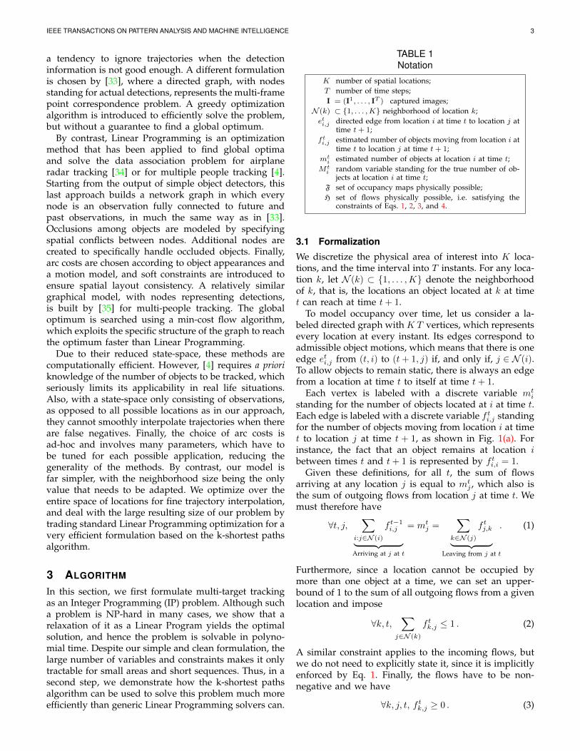
TABLE 1Notation

K number of spatial locations;T number of time steps;I = (I1, . . . , IT ) captured images;

N (k) ⊂ {1, . . . ,K} neighborhood of location k;eti,j directed edge from location i at time t to location j at

time t+ 1;f ti,j estimated number of objects moving from location i at

time t to location j at time t+ 1;mt

i estimated number of objects at location i at time t;Mt

i random variable standing for the true number of ob-jects at location i at time t;

F set of occupancy maps physically possible;H set of flows physically possible, i.e. satisfying the

constraints of Eqs. 1, 2, 3, and 4.

3.1 Formalization

We discretize the physical area of interest into K loca-tions, and the time interval into T instants. For any loca-tion k, let N (k) ⊂ {1, . . . ,K} denote the neighborhoodof k, that is, the locations an object located at k at timet can reach at time t+ 1.

To model occupancy over time, let us consider a la-beled directed graph with K T vertices, which representsevery location at every instant. Its edges correspond toadmissible object motions, which means that there is oneedge eti,j from (t, i) to (t+ 1, j) if, and only if, j ∈ N (i).To allow objects to remain static, there is always an edgefrom a location at time t to itself at time t+ 1.

Each vertex is labeled with a discrete variable mti

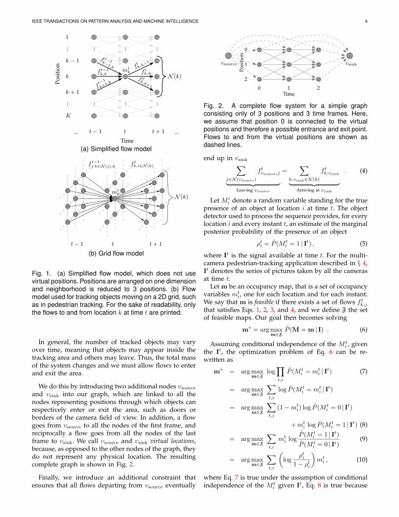
standing for the number of objects located at i at time t.Each edge is labeled with a discrete variable f ti,j standingfor the number of objects moving from location i at timet to location j at time t + 1, as shown in Fig. 1(a). Forinstance, the fact that an object remains at location ibetween times t and t+ 1 is represented by f ti,i = 1.

Given these definitions, for all t, the sum of flowsarriving at any location j is equal to mt

j , which also isthe sum of outgoing flows from location j at time t. Wemust therefore have

∀t, j,∑

i:j∈N (i)

f t−1i,j︸︷︷︸Arriving at j at t

= mtj =

∑k∈N (j)

f tj,k︸︷︷︸Leaving from j at t

. (1)

Furthermore, since a location cannot be occupied bymore than one object at a time, we can set an upper-bound of 1 to the sum of all outgoing flows from a givenlocation and impose

∀k, t,∑

j∈N (k)

f tk,j ≤ 1 . (2)

A similar constraint applies to the incoming flows, butwe do not need to explicitly state it, since it is implicitlyenforced by Eq. 1. Finally, the flows have to be non-negative and we have

∀k, j, t, f tk,j ≥ 0 . (3)


k + 1

k

k − 1

1

K

......

Posi

tion

...

f tk,kf t−1

k,kmt

k

... ............

f t−1k−1,k

ft−1k+

1,kf tk,k+1

ftk,k−1

N (k)

t− 1 t+ 1 ...... t

Time(a) Simplified flow model

t− 1 t t+ 1

mtk N (k)

f t−1j:k∈N (j),k f t

k,i∈N (k)

(b) Grid flow model

Fig. 1. (a) Simplified flow model, which does not usevirtual positions. Positions are arranged on one dimensionand neighborhood is reduced to 3 positions. (b) Flowmodel used for tracking objects moving on a 2D grid, suchas in pedestrian tracking. For the sake of readability, onlythe flows to and from location k at time t are printed.

In general, the number of tracked objects may varyover time, meaning that objects may appear inside thetracking area and others may leave. Thus, the total massof the system changes and we must allow flows to enterand exit the area.

We do this by introducing two additional nodes υsourceand υsink into our graph, which are linked to all thenodes representing positions through which objects canrespectively enter or exit the area, such as doors orborders of the camera field of view. In addition, a flowgoes from υsource to all the nodes of the first frame, andreciprocally a flow goes from all the nodes of the lastframe to υsink. We call υsource and υsink virtual locations,because, as opposed to the other nodes of the graph, theydo not represent any physical location. The resultingcomplete graph is shown in Fig. 2.

Finally, we introduce an additional constraint thatensures that all flows departing from υsource eventually

υsink

0

1

2

Posi

tion

0 1 2Time

υsource

Fig. 2. A complete flow system for a simple graphconsisting only of 3 positions and 3 time frames. Here,we assume that position 0 is connected to the virtualpositions and therefore a possible entrance and exit point.Flows to and from the virtual positions are shown asdashed lines.

end up in υsink∑j∈N (υsource)

f tυsource,j︸︷︷︸Leaving υsource

=∑

k:υsink∈N (k)

f tk,υsink︸︷︷︸Arriving at υsink

. (4)

Let M ti denote a random variable standing for the true

presence of an object at location i at time t. The objectdetector used to process the sequence provides, for everylocation i and every instant t, an estimate of the marginalposterior probability of the presence of an object

ρti = P (M ti = 1 | It) , (5)

where It is the signal available at time t. For the multi-camera pedestrian-tracking application described in § 4,It denotes the series of pictures taken by all the camerasat time t.

Let m be an occupancy map, that is a set of occupancyvariables mt

i, one for each location and for each instant.We say that m is feasible if there exists a set of flows f tk,jthat satisfies Eqs. 1, 2, 3, and 4, and we define F the setof feasible maps. Our goal then becomes solving

m∗ = argmaxm∈F

P (M = m | I) . (6)

Assuming conditional independence of the M ti , given

the It, the optimization problem of Eq. 6 can be re-written as

m∗ = argmaxm∈F

log∏t,i

P (M ti = mt

i | It) (7)

= argmaxm∈F

∑t,i

log P (M ti = mt

i | It)

= argmaxm∈F

∑t,i

(1−mti) log P (M

ti = 0 | It)

+mti log P (M

ti = 1 | It) (8)

= argmaxm∈F

∑t,i

mti log

P (M ti = 1 | It)

P (M ti = 0 | It)

(9)

= argmaxm∈F

∑t,i

(log

ρti1− ρti

)mti , (10)

where Eq. 7 is true under the assumption of conditionalindependence of the M t

i given It, Eq. 8 is true because


mti is 0 or 1 according to Eq. 2, and Eq. 9 is obtained by

ignoring a term which does not depend on m. Hence,the objective function of Eq. 10 is a linear expression ofthe mt

i.

3.2 Linear Programming FormulationThe formulation defined above translates naturally intothe Integer Program

Maximize∑t,i

log

(ρti

1− ρti

) ∑j∈N (i)

f ti,j

subject to ∀t, i, j, f ti,j ≥ 0

∀t, i,∑

j∈N (i)

f ti,j ≤ 1

∀t, i,∑

j∈N (i)

f ti,j −∑

k:i∈N (k)

f t−1k,i ≤ 0

∑j∈N (υsource)

fυsource,j −∑

k:υsink∈N (k)

fk,υsink≤ 0 .

(11)

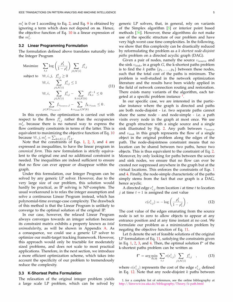
In this system, the optimization is carried out withrespect to the flows f ti,j rather than the occupanciesmti, because there is no natural way to express the

flow continuity constraints in terms of the latter. This isequivalent to maximizing the objective function of Eq. 10because ∀t, j,mt

j =∑k∈N (j) f

tj,k.

Note that the constraints of Eqs. 1, 2, 3, and 4 areexpressed as inequalities, to have the linear program incanonical form. This new formulation is strictly equiva-lent to the original one and no additional constraint isneeded. The inequalities are indeed sufficient to ensurethat no flow can ever appear or disappear within thegraph.

Under this formulation, our Integer Program can besolved by any generic LP solver. However, due to thevery large size of our problem, this solution wouldhardly be practical, as IP solving is NP-complete. Theusual workaround is to relax the integer assumption andsolve a continuous Linear Program instead, which haspolynomial-time average-case complexity. The drawbackof this method is that the Linear Program is unlikely toconverge to the optimal solution of the original IP.

In our case, however, the relaxed Linear Programalways converges towards an integer solution becauseits constraint matrix exhibits a property known as totalunimodularity, as will be shown in Appendix A. Asa consequence, we could use a generic LP solver tooptimize our multi-target tracking framework. However,this approach would only be tractable for moderatelysized problems, and does not scale to most practicalapplications. Therefore, in the next section, we introducea more efficient optimization scheme, which takes intoaccount the specificity of our problem to tremendouslyreduce the complexity.

3.3 K-Shortest Paths FormulationThe relaxation of the original integer problem yieldsa large scale LP problem, which can be solved by

generic LP solvers, that, in general, rely on variantsof the Simplex algorithm [5] or interior point basedmethods [36]. However, these algorithms do not makeuse of the specific structure of our problem and havevery high worst case time complexities. In the following,we show that this complexity can be drastically reducedby reformulating the problem as a k shortest node-disjointpaths problem on a directed acyclic graph (DAG).

Given a pair of nodes, namely the source υsource andthe sink υsink, in a graph G, the k-shortest paths problemis to find the k paths {p1, . . . , pk} between these nodes,such that the total cost of the paths is minimum. Theproblem is well-studied in the network optimizationliterature and the results have been widely applied inthe field of network connection routing and restoration.There exists many variants of the algorithm, each tar-geted at a specific problem instance 1.

In our specific case, we are interested in the partic-ular instance where the graph is directed and pathsare both node-disjoint - i.e. two separate paths cannotshare the same node - and node-simple - i.e. a pathvisits every node in the graph at most once. We usethe graph structure with a single source and a singlesink illustrated by Fig. 2. Any path between υsourceand υsink in this graph represents the flow of a singleobject in the original problem along the edges of thepath. The node-disjointness constraint means that nolocation can be shared between two paths, hence twoobjects. This is thus equivalent to the constraint of Eq. 2.Moreover, by only looking for paths between the sourceand sink nodes, we ensure that no flow can ever becreated nor suppressed anywhere in the graph but at thevirtual locations. This enforces the constraints of Eqs. 1and 4. Finally, the node-simple characteristic of the pathssimply stems from the fact that our graph is a DAG,hence acyclic.

A directed edge eti,j from location i at time t to locationj at time t+ 1 is assigned the cost value

c(eti,j) = − log

(ρti

1− ρti

). (12)

The cost value of the edges emanating from the sourcenode is set to zero to allow objects to appear at anyentrance position and at any time instant at no cost. Weformulate our problem as a minimization problem bynegating the objective function of Eq. 11.

Let H denote the set of feasible solutions of the originalLP formulation of Eq. 11, satisfying the constraints givenin Eq. 1, 2, 3, and 4. Then, the optimal solution f∗ of thek-shortest paths problem can be written as

f∗ = argminf∈H

∑t,i

c(eti,j)∑

j∈N (i)

f ti,j , (13)

where c(eti,j) represents the cost of the edge eti,j definedin Eq. 12. Note that any node-disjoint k paths between

1. for a complete list of references, see the online bibliography athttp://liinwww.ira.uka.de/bibliography/Theory/k-path.html

http://liinwww.ira.uka.de/bibliography/Theory/k-path.html


υsource and υsink with arbitrary k is in the feasible setof solutions H. In addition, any solution in H can beexpressed as a set of k node-disjoint paths.

Let p∗i be the shortest path computed at the ith itera-tion of the algorithm and Pl = {p∗1, . . . , p∗l } be the set ofall l shortest paths computed up to iteration l. We startby finding the single shortest path in the graph p∗1 andcompute its total cost

cost(p∗l ) =∑

eti,j∈p∗l

c(eti,j) . (14)

We then compute iteratively the l-shortest paths for l =2, 3, 4, . . ., and for each l, we calculate the total cost ofthe shortest paths

cost(Pl) =

l∑i=1

cost(p∗i ) . (15)

At each new iteration l + 1, the total cost cost(Pl+1) iscompared to the cost at the previous iteration cost(Pl).The optimal number of paths k∗ is obtained when thecost of iteration k∗+1 is higher than the one of iterationk∗. The procedure is summarized by the pseudo-code ofAlgorithm 1, in Appendix B.

To compute such k-shortest paths, we use the disjointpaths algorithm [6], which is an efficient iterative methodbased on signed paths. For the sake of completeness, wegive a brief description of this algorithm in Appendix B.

The equivalence of the LP and the k-shortest pathsformulations follows from the exact procedure we useto select an optimal k such that the objective function isminimized. Since path costs are monotonically increas-ing

cost(p∗i+1) ≥ cost(p∗i ) ∀i , (16)

the total cost function cost(Pl) is convex with respect to l.Therefore, the global minimum is reached when cost(p∗i )changes sign and becomes non-negative

cost(Pk∗−1) ≥ cost(Pk∗) ≤ cost(Pk∗+1) . (17)

This is set as the stopping criterion of the algorithm, aspresented in Algorithm 1. Finally, among the set of allconsecutive values that may satisfy the above condition,we select the smallest one to avoid erroneous splittingof paths.

As discussed in Appendix B, the worst case complex-ity of the algorithm is O(k(m+n · log n)), where k is thenumber of objects appearing in a given time interval,m is the number of edges and n the number of nodesin the final transformed graph. This is more efficientthan the min-cost flow method of [35], which exhibitsa worst case complexity of O(kn2m log n). Furthermore,due to the mostly acyclic nature of our graph, theaverage complexity is almost linear with the number ofnodes, which is reflected by our experimental results inFig. 7(b). This is much faster than general LP solvers,and a speed gain of up to a factor 1,000 can be expected,as illustrated by the run time comparison in §4.10.

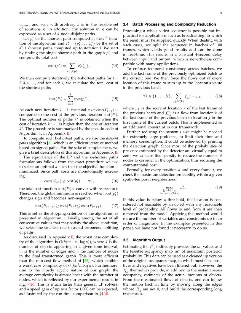
3.4 Batch Processing and Complexity Reduction

Processing a whole video sequence is possible but im-practical for applications such as broadcasting, in whichthe result must be supplied quickly. When dealing withsuch cases, we split the sequence in batches of 100frames, which yields good results and can be donein real-time. This results in a constant 4-second delaybetween input and output, which is nevertheless com-patible with many applications.

To enforce temporal consistency across batches, weadd the last frame of the previously optimized batch tothe current one. We then force the flows out of everylocation of this frame to sum up to the location’s valuein the previous batch

∀k ∈ {1, . . . ,K},∑

j∈N (k)

f−1k,j = µk, (18)

where µk is the score at location k of the last frame ofthe previous batch and f−1k,j is a flow from location k ofthe last frame of the previous batch to location j in thefirst frame of the current batch. This is implemented asan additional constraint in our framework.

Further reducing the system’s size might be neededfor extremely large problems, to limit their time andmemory consumption. It could be achieved by pruningthe detection graph. Since most of the probabilities ofpresence estimated by the detector are virtually equal tozero, we can use this sparsity to reduce the number ofnodes to consider in the optimization, thus reducing thecomputational cost.

Formally, for every position k and every frame t, wecheck the maximum detection probability within a givenspatio-temporal neighborhood

max‖j−k‖<τ1

t−τ2<u<t+τ2

ρuj . (19)

If this value is below a threshold, the location is con-sidered not reachable by an object with any reasonablelevel of probability. All flows to and from it are thenremoved from the model. Applying this method wouldreduce the number of variables and constraints up to anorder of magnitude. In the examples presented in thispaper, we have not found it necessary to do so.

3.5 Algorithm Output

Estimating the f ti,j indirectly provides the mti values and

the feasible occupancy map m∗ of maximum posteriorprobability. This data can be used as a cleaned up versionof the original occupancy map, in which most false posi-tives and negatives have been filtered out. However, thef ti,j themselves provide, in addition to the instantaneousoccupancy, estimates of the actual motions of objects.From these estimated flows of objects, one can followthe motion back in time by moving along the edgeswhose f ti,j are not 0, and build the corresponding longtrajectories.


4 RESULTSIn this section, we present results in two very differentcontexts. First, we use a multi-camera setup in which thecameras are located at shoulder level to track pedestrianswho may walk in front of each other. The frequentocclusions between people produce noisy detections,which our algorithm nevertheless links very reliably. Asa result, our approach was shown to compare favorablyagainst other state-of-the-art algorithms in the PETS 2009evaluation [37]. Second, to highlight the fact that wedo not depend on an appearance model, we track setsof similar-looking bouncing balls seen from above. Inboth cases, we compare our results to those of ourearlier tracking method based on sequential DynamicProgramming [3], and show that we can obtain goodresults even when using a single camera.

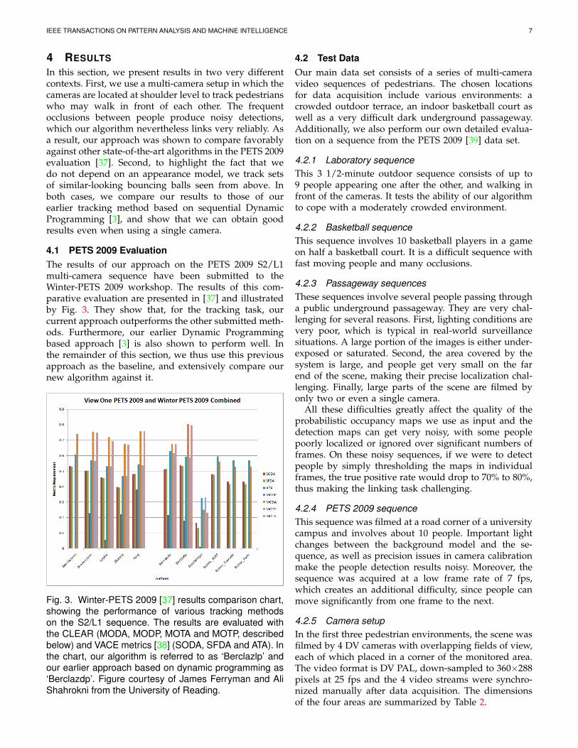
4.1 PETS 2009 EvaluationThe results of our approach on the PETS 2009 S2/L1multi-camera sequence have been submitted to theWinter-PETS 2009 workshop. The results of this com-parative evaluation are presented in [37] and illustratedby Fig. 3. They show that, for the tracking task, ourcurrent approach outperforms the other submitted meth-ods. Furthermore, our earlier Dynamic Programmingbased approach [3] is also shown to perform well. Inthe remainder of this section, we thus use this previousapproach as the baseline, and extensively compare ournew algorithm against it.

Fig. 3. Winter-PETS 2009 [37] results comparison chart,showing the performance of various tracking methodson the S2/L1 sequence. The results are evaluated withthe CLEAR (MODA, MODP, MOTA and MOTP, describedbelow) and VACE metrics [38] (SODA, SFDA and ATA). Inthe chart, our algorithm is referred to as ‘Berclazlp’ andour earlier approach based on dynamic programming as‘Berclazdp’. Figure courtesy of James Ferryman and AliShahrokni from the University of Reading.

4.2 Test DataOur main data set consists of a series of multi-cameravideo sequences of pedestrians. The chosen locationsfor data acquisition include various environments: acrowded outdoor terrace, an indoor basketball court aswell as a very difficult dark underground passageway.Additionally, we also perform our own detailed evalua-tion on a sequence from the PETS 2009 [39] data set.

4.2.1 Laboratory sequenceThis 3 1/2-minute outdoor sequence consists of up to9 people appearing one after the other, and walking infront of the cameras. It tests the ability of our algorithmto cope with a moderately crowded environment.

4.2.2 Basketball sequenceThis sequence involves 10 basketball players in a gameon half a basketball court. It is a difficult sequence withfast moving people and many occlusions.

4.2.3 Passageway sequencesThese sequences involve several people passing througha public underground passageway. They are very chal-lenging for several reasons. First, lighting conditions arevery poor, which is typical in real-world surveillancesituations. A large portion of the images is either under-exposed or saturated. Second, the area covered by thesystem is large, and people get very small on the farend of the scene, making their precise localization chal-lenging. Finally, large parts of the scene are filmed byonly two or even a single camera.

All these difficulties greatly affect the quality of theprobabilistic occupancy maps we use as input and thedetection maps can get very noisy, with some peoplepoorly localized or ignored over significant numbers offrames. On these noisy sequences, if we were to detectpeople by simply thresholding the maps in individualframes, the true positive rate would drop to 70% to 80%,thus making the linking task challenging.

4.2.4 PETS 2009 sequenceThis sequence was filmed at a road corner of a universitycampus and involves about 10 people. Important lightchanges between the background model and the se-quence, as well as precision issues in camera calibrationmake the people detection results noisy. Moreover, thesequence was acquired at a low frame rate of 7 fps,which creates an additional difficulty, since people canmove significantly from one frame to the next.

4.2.5 Camera setupIn the first three pedestrian environments, the scene wasfilmed by 4 DV cameras with overlapping fields of view,each of which placed in a corner of the monitored area.The video format is DV PAL, down-sampled to 360×288pixels at 25 fps and the 4 video streams were synchro-nized manually after data acquisition. The dimensionsof the four areas are summarized by Table 2.


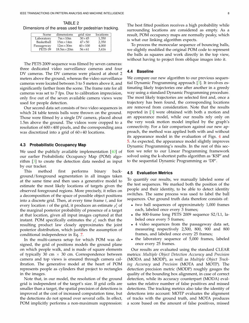
TABLE 2Dimensions of the areas used for pedestrian tracking.

Scene dimensions grid size locationsLaboratory 7m×10m 30×45 1,350Basketball 15m×14m 47×50 2,350

Passageway 12m×30m 40×100 4,000PETS 09 18.5m×20m 56×61 3,416

The PETS 2009 sequence was filmed by seven cameras:three dedicated video surveillance cameras and fourDV cameras. The DV cameras were placed at about 2meters above the ground, whereas the video surveillancecameras were located between 3 to 5 meters above it, andsignificantly farther from the scene. The frame rate for allcameras was set to 7 fps. Due to calibration imprecision,only five out of the seven available camera views wereused for people detection.

Our second data set consists of two video sequences inwhich 24 table tennis balls were thrown on the ground.Those were filmed by a single DV camera, placed about1.5m above the ground. The videos were cropped to aresolution of 600×400 pixels, and the corresponding areawas discretized into a grid of 60×40 locations.

4.3 Probabilistic Occupancy Map

We used the publicly available implementation [40] ofour earlier Probabilistic Occupancy Map (POM) algo-rithm [3] to create the detection data needed as inputby our tracker.

This method first performs binary back-ground/foreground segmentation in all images takenat the same time and then uses a generative model toestimate the most likely locations of targets given theobserved foreground regions. More precisely, it relies ona decomposition of the space of possible object positionsinto a discrete grid. Then, at every time frame t, and forevery location i of the grid, it produces an estimate ρti ofthe marginal posterior probability of presence of a targetat that location, given all input images captured at thatinstant. POM specifically estimates the ρti such that theresulting product law closely approximates the jointposterior distribution, which justifies the assumption ofconditional independence in Eq. 7.

In the multi-camera setup for which POM was de-signed, the grid of positions models the ground planeon which people walk, and is made of square elementsof typically 30 cm × 30 cm. Correspondence betweencamera and top views is ensured through camera cal-ibration. The generative model at the heart of POMrepresents people as cylinders that project to rectanglesin the images.

Note that, in our model, the resolution of the groundgrid is independent of the target’s size. If grid cells aresmaller than a target, the spatial precision of detections isimproved at the cost of increased computation time, butthe detections do not spread over several cells. In effect,POM implicitly performs a non-maximum suppression:

The best fitted position receives a high probability whilesurrounding locations are considered as empty. As aresult, POM occupancy maps are normally peaky, whichis what our linking algorithm expects.

To process the monocular sequence of bouncing balls,we slightly modified the original POM code to representthe balls as squares and work directly in the top view,without having to project from oblique images into it.

4.4 Baseline

We compare our new algorithm to our previous sequen-tial Dynamic Programming approach [3]. It involves es-timating likely trajectories one after another in a greedyway using a standard Dynamic Programming procedure.The most likely trajectories are selected first and, once atrajectory has been found, the corresponding locationsare removed from consideration. Note that the resultsreported in [3] were obtained with both a motion andan appearance model, while our results rely only onthe very weak motion model implied by the graph’sconnectivity. For a fair comparison against our new ap-proach, the method was applied both with and withoutits appearance model in the evaluation of Figs. 4 and5. As expected, the appearance model slightly improvesDynamic Programming’s results. In the rest of this sec-tion we refer to our Linear Programming frameworksolved using the k-shortest paths algorithm as ‘KSP’ andto the sequential Dynamic Programming as ‘DP’.

4.5 Evaluation Metrics

To quantify our results, we manually labeled some ofthe test sequences. We marked both the position of thepeople and their identity, to be able to detect identityswitches. The same process was used to label the ballsequences. Our ground truth data therefore consists of:• two ball sequences of approximately 1,000 frames

each, labeled once every 3 frames;• the 800-frame long PETS 2009 sequence S2/L1, la-

beled once every 5 frames;• 4 video sequences from the passageway data set,

measuring respectively 2,500, 800, 900 and 800frames, and labeled once every 25 frames;

• the laboratory sequence of 5,000 frames, labeledonce every 25 frames.

Our results are evaluated using the standard CLEARmetrics: Multiple Object Detection Accuracy and Precision(MODA and MODP), as well as Multiple Object Track-ing Accuracy and Precision (MOTA and MOTP). Thedetection precision metric (MODP) roughly gauges thequality of the bounding box alignment, in case of correctdetection, while its accuracy counterpart (MODA) eval-uates the relative number of false positives and misseddetections. The tracking metrics also take the identity ofdetections into account: MOTP evaluates the alignmentof tracks with the ground truth, and MOTA producesa score based on the amount of false positives, missed


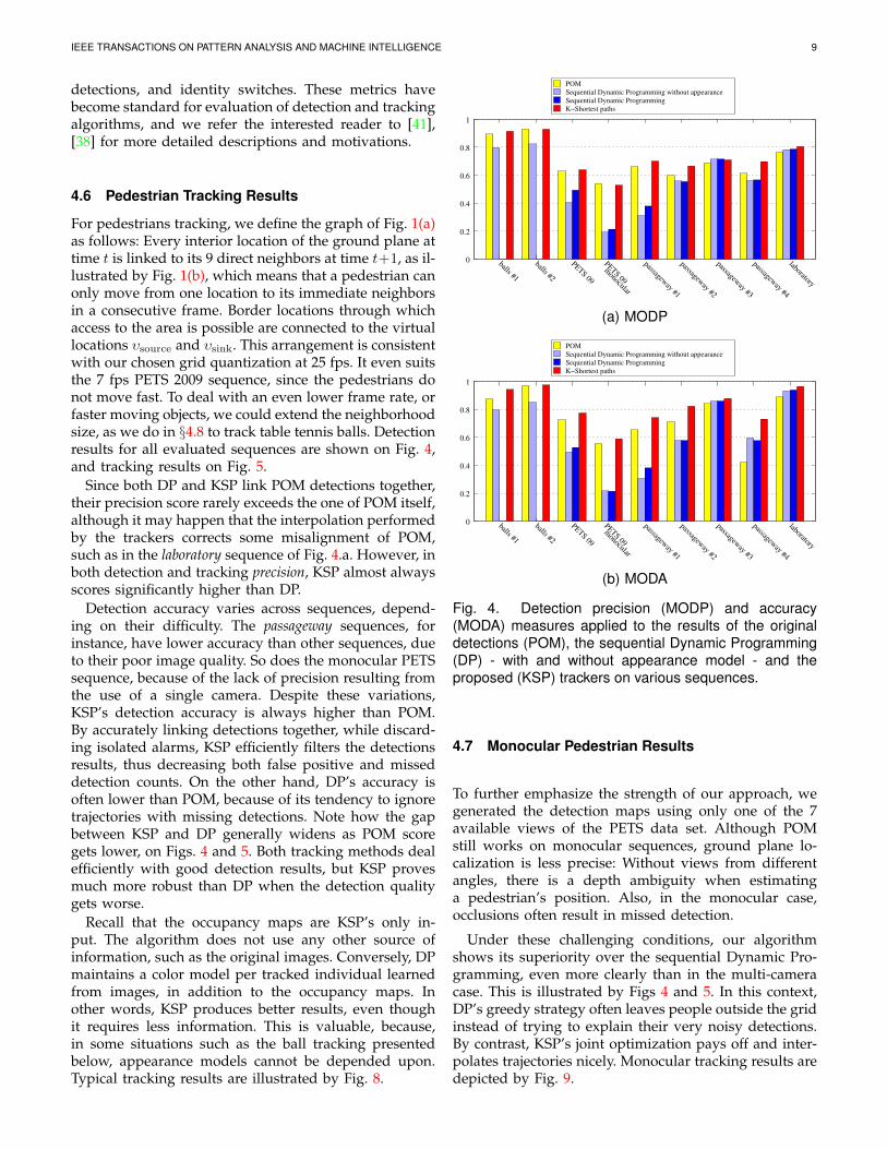
detections, and identity switches. These metrics havebecome standard for evaluation of detection and trackingalgorithms, and we refer the interested reader to [41],[38] for more detailed descriptions and motivations.

4.6 Pedestrian Tracking Results

For pedestrians tracking, we define the graph of Fig. 1(a)as follows: Every interior location of the ground plane attime t is linked to its 9 direct neighbors at time t+1, as il-lustrated by Fig. 1(b), which means that a pedestrian canonly move from one location to its immediate neighborsin a consecutive frame. Border locations through whichaccess to the area is possible are connected to the virtuallocations υsource and υsink. This arrangement is consistentwith our chosen grid quantization at 25 fps. It even suitsthe 7 fps PETS 2009 sequence, since the pedestrians donot move fast. To deal with an even lower frame rate, orfaster moving objects, we could extend the neighborhoodsize, as we do in §4.8 to track table tennis balls. Detectionresults for all evaluated sequences are shown on Fig. 4,and tracking results on Fig. 5.

Since both DP and KSP link POM detections together,their precision score rarely exceeds the one of POM itself,although it may happen that the interpolation performedby the trackers corrects some misalignment of POM,such as in the laboratory sequence of Fig. 4.a. However, inboth detection and tracking precision, KSP almost alwaysscores significantly higher than DP.

Detection accuracy varies across sequences, depend-ing on their difficulty. The passageway sequences, forinstance, have lower accuracy than other sequences, dueto their poor image quality. So does the monocular PETSsequence, because of the lack of precision resulting fromthe use of a single camera. Despite these variations,KSP’s detection accuracy is always higher than POM.By accurately linking detections together, while discard-ing isolated alarms, KSP efficiently filters the detectionsresults, thus decreasing both false positive and misseddetection counts. On the other hand, DP’s accuracy isoften lower than POM, because of its tendency to ignoretrajectories with missing detections. Note how the gapbetween KSP and DP generally widens as POM scoregets lower, on Figs. 4 and 5. Both tracking methods dealefficiently with good detection results, but KSP provesmuch more robust than DP when the detection qualitygets worse.

Recall that the occupancy maps are KSP’s only in-put. The algorithm does not use any other source ofinformation, such as the original images. Conversely, DPmaintains a color model per tracked individual learnedfrom images, in addition to the occupancy maps. Inother words, KSP produces better results, even thoughit requires less information. This is valuable, because,in some situations such as the ball tracking presentedbelow, appearance models cannot be depended upon.Typical tracking results are illustrated by Fig. 8.

0

0.2

0.4

0.6

0.8

1

balls #1

balls #2

PETS 09

PETS 09

monocular

passageway #1

passageway #2

passageway #3

passageway #4

laboratory

POM

Sequential Dynamic Programming without appearance

Sequential Dynamic Programming

K−Shortest paths

(a) MODP

0

0.2

0.4

0.6

0.8

1

balls #1

balls #2

PETS 09

PETS 09

monocular

passageway #1

passageway #2

passageway #3

passageway #4

laboratory

POM



K−Shortest paths

(b) MODA

Fig. 4. Detection precision (MODP) and accuracy(MODA) measures applied to the results of the originaldetections (POM), the sequential Dynamic Programming(DP) - with and without appearance model - and theproposed (KSP) trackers on various sequences.

4.7 Monocular Pedestrian Results

To further emphasize the strength of our approach, wegenerated the detection maps using only one of the 7available views of the PETS data set. Although POMstill works on monocular sequences, ground plane lo-calization is less precise: Without views from differentangles, there is a depth ambiguity when estimatinga pedestrian’s position. Also, in the monocular case,occlusions often result in missed detection.

Under these challenging conditions, our algorithmshows its superiority over the sequential Dynamic Pro-gramming, even more clearly than in the multi-cameracase. This is illustrated by Figs 4 and 5. In this context,DP’s greedy strategy often leaves people outside the gridinstead of trying to explain their very noisy detections.By contrast, KSP’s joint optimization pays off and inter-polates trajectories nicely. Monocular tracking results aredepicted by Fig. 9.


0

0.2

0.4

0.6

0.8

1

balls #1

balls #2

PETS 09

PETS 09

monocular

passageway #1

passageway #2

passageway #3

passageway #4

laboratory



K−Shortest paths

(a) MOTP

0

0.2

0.4

0.6

0.8

1

balls #1

balls #2

PETS 09

PETS 09

monocular

passageway #1

passageway #2

passageway #3

passageway #4

laboratory



K−Shortest paths

(b) MOTA

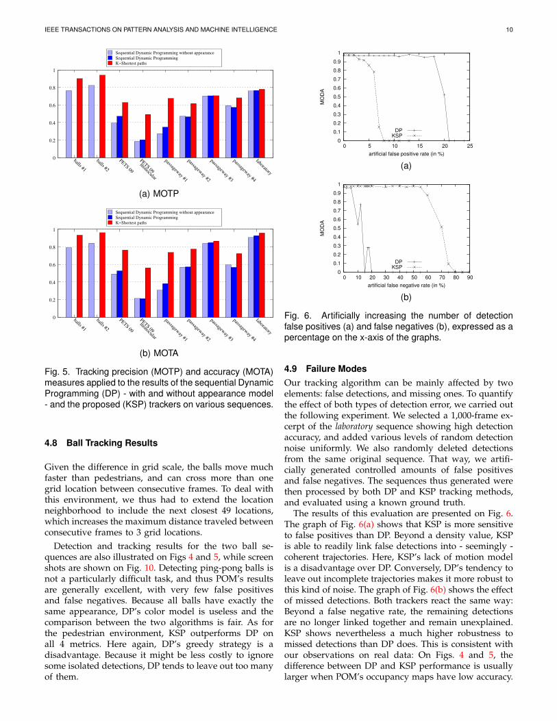
Fig. 5. Tracking precision (MOTP) and accuracy (MOTA)measures applied to the results of the sequential DynamicProgramming (DP) - with and without appearance model- and the proposed (KSP) trackers on various sequences.

4.8 Ball Tracking Results

Given the difference in grid scale, the balls move muchfaster than pedestrians, and can cross more than onegrid location between consecutive frames. To deal withthis environment, we thus had to extend the locationneighborhood to include the next closest 49 locations,which increases the maximum distance traveled betweenconsecutive frames to 3 grid locations.

Detection and tracking results for the two ball se-quences are also illustrated on Figs 4 and 5, while screenshots are shown on Fig. 10. Detecting ping-pong balls isnot a particularly difficult task, and thus POM’s resultsare generally excellent, with very few false positivesand false negatives. Because all balls have exactly thesame appearance, DP’s color model is useless and thecomparison between the two algorithms is fair. As forthe pedestrian environment, KSP outperforms DP onall 4 metrics. Here again, DP’s greedy strategy is adisadvantage. Because it might be less costly to ignoresome isolated detections, DP tends to leave out too manyof them.

0

0.1

0.2

0.3

0.4

0.5

0.6

0.7

0.8

0.9

1

0 5 10 15 20 25

MO

DA

artificial false positive rate (in %)

DP KSP

(a)

0

0.1

0.2

0.3

0.4

0.5

0.6

0.7

0.8

0.9

1

0 10 20 30 40 50 60 70 80 90

MO

DA

artificial false negative rate (in %)

DP KSP

(b)

Fig. 6. Artificially increasing the number of detectionfalse positives (a) and false negatives (b), expressed as apercentage on the x-axis of the graphs.

4.9 Failure ModesOur tracking algorithm can be mainly affected by twoelements: false detections, and missing ones. To quantifythe effect of both types of detection error, we carried outthe following experiment. We selected a 1,000-frame ex-cerpt of the laboratory sequence showing high detectionaccuracy, and added various levels of random detectionnoise uniformly. We also randomly deleted detectionsfrom the same original sequence. That way, we artifi-cially generated controlled amounts of false positivesand false negatives. The sequences thus generated werethen processed by both DP and KSP tracking methods,and evaluated using a known ground truth.

The results of this evaluation are presented on Fig. 6.The graph of Fig. 6(a) shows that KSP is more sensitiveto false positives than DP. Beyond a density value, KSPis able to readily link false detections into - seemingly -coherent trajectories. Here, KSP’s lack of motion modelis a disadvantage over DP. Conversely, DP’s tendency toleave out incomplete trajectories makes it more robust tothis kind of noise. The graph of Fig. 6(b) shows the effectof missed detections. Both trackers react the same way:Beyond a false negative rate, the remaining detectionsare no longer linked together and remain unexplained.KSP shows nevertheless a much higher robustness tomissed detections than DP does. This is consistent withour observations on real data: On Figs. 4 and 5, thedifference between DP and KSP performance is usuallylarger when POM’s occupancy maps have low accuracy.


Another problem to which our method is potentiallyvulnerable is identity switch. Since we rely entirely ondetection data and do not use any appearance infor-mation nor complex motion model, there is no way todistinguish two trajectories intersecting. In practice, wedo not suffer much from this, because most of the time,the objects evolve outside of each other’s neighborhood.Moreover, the joint optimization of all trajectories paysoff in this regard, as opposed to DP’s greedy strategy.

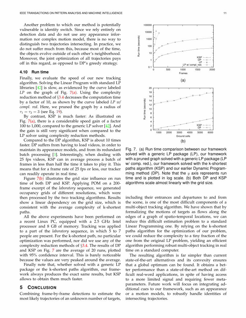
4.10 Run timeFinally, we evaluate the speed of our new trackingalgorithm. Solving the Linear Program with standard LPlibraries [42] is slow, as evidenced by the curve labeledLP on the graph of Fig. 7(a). Using the complexityreduction method of §3.4 decreases the computation timeby a factor of 10, as shown by the curve labeled LP w/compl. red. Here, we pruned the graph by a radius ofτ1 = τ2 = 3 (see Eq. 19).

By contrast, KSP is much faster: As illustrated onFig. 7(a), there is a considerable speed gain of a factor100 to 1,000, compared to the generic LP solver [42]. Andthe gain is still very significant when compared to theLP solver using complexity reduction methods.

Compared to the DP algorithm, KSP is about 10 timesfaster. DP suffers from having to load videos, in order tomaintain its appearance models, and from its redundantbatch processing [3]. Interestingly, when dealing with25 fps videos, KSP can in average process a batch offrames in less than half the time it takes to play it. Thismeans that for a frame rate of 25 fps or less, our trackercan readily operate in real time.

Figure 7(b) illustrates the grid size influence on runtime of both DP and KSP. Applying POM on a 200-frame excerpt of the laboratory sequence, we generatedoccupancy grids of different resolutions, which werethen processed by the two tracking algorithms. Resultsshow a linear dependency on the grid size, which isconsistent with the average complexity of k-shortestpaths.

All the above experiments have been performed ona recent Linux PC, equipped with a 2.5 GHz Intelprocessor and 8 GB of memory. Tracking was appliedto a part of the laboratory sequence, in which 5 to 7people are present. For the k-shortest path, no particularoptimization was performed, nor did we use any of thecomplexity reduction methods of §3.4. The results of DPand KSP on Fig. 7 are the average of 20 runs, plottedwith 95% confidence interval. This is barely noticeablebecause the values are very peaked around the average.

Finally note that, whether solved with a generic LPpackage or the k-shortest paths algorithm, our frame-work always produces the exact same results, but KSPallows to obtain them much faster.

5 CONCLUSIONCombining frame-by-frame detections to estimate themost likely trajectories of an unknown number of targets,

0.1

1

10

100

1000

10000

100000

0 500 1000 1500 2000

Run tim

e (

seconds)

Frames

KSPDP LP

LP w/ compl. red.

(a)

0

2

4

6

8

10

12

14

16

18

20

1000 2000 3000 4000 5000 6000

Run tim

e (

seconds)

Ground cells

KSPDP

(b)

Fig. 7. (a) Run time comparison between our frameworksolved with a generic LP package (LP), our frameworkwith a pruned graph solved with a generic LP package (LPw/ comp. red.), our framework solved with the k-shortestpaths algorithm (KSP) and our earlier Dynamic Program-ming method (DP). Note that the y axis represents runtime and is plotted in log scale. (b) Both DP and KSPalgorithms scale almost linearly with the grid size.

including their entrances and departures to and fromthe scene, is one of the most difficult components of amulti-object tracking algorithm. We have shown that byformalizing the motions of targets as flows along theedges of a graph of spatio-temporal locations, we canreduce this difficult estimation problem to a standardLinear Programming one. By relying on the k-shortestpaths algorithm for the optimization of our problem,we could reduce the complexity to a tiny fraction of theone from the original LP problem, yielding an efficientalgorithm performing robust multi-object tracking in realtime on a standard computer.

The resulting algorithm is far simpler than currentstate-of-the-art alternatives and its convexity ensuresthat a global optimum can be found. It obtains a bet-ter performance than a state-of-the-art method on dif-ficult real-word applications, in spite of having accessto a more limited signal and requiring fewer meta-parameters. Future work will focus on integrating ad-ditional cues to our framework, such as an appearanceor a motion models, to robustly handle identities ofintersecting trajectories.


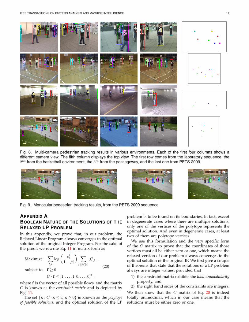
Fig. 8. Multi-camera pedestrian tracking results in various environments. Each of the first four columns shows adifferent camera view. The fifth column displays the top view. The first row comes from the laboratory sequence, the2nd from the basketball environment, the 3rd from the passageway, and the last one from PETS 2009.

Fig. 9. Monocular pedestrian tracking results, from the PETS 2009 sequence.

APPENDIX ABOOLEAN NATURE OF THE SOLUTIONS OF THERELAXED LP PROBLEMIn this appendix, we prove that, in our problem, theRelaxed Linear Program always converges to the optimalsolution of the original Integer Program. For the sake ofthe proof, we rewrite Eq. 11 in matrix form as

Maximize∑t,i

log

(ρti

1− ρti

) ∑j∈N (i)

f ti,j ,

subject to f ≥ 0

C · f ≤ [1, . . . , 1, 0, . . . , 0]T,

(20)

where f is the vector of all possible flows, and the matrixC is known as the constraint matrix and is depicted byFig. 11.

The set {x : C · x ≤ b, x ≥ 0} is known as the polytopeof feasible solutions, and the optimal solution of the LP

problem is to be found on its boundaries. In fact, exceptin degenerate cases where there are multiple solutions,only one of the vertices of the polytope represents theoptimal solution. And even in degenerate cases, at leasttwo of them are polytope vertices.

We use this formulation and the very specific formof the C matrix to prove that the coordinates of thosevertices must all be either zero or one, which means therelaxed version of our problem always converges to theoptimal solution of the original IP. We first give a coupleof theorems that state that the solutions of a LP problemalways are integer values, provided that

1) the constraint matrix exhibits the total unimodularityproperty, and

2) the right hand sides of the constraints are integers.

We then show that the C matrix of Eq. 20 is indeedtotally unimodular, which in our case means that thesolutions must be either zero or one.


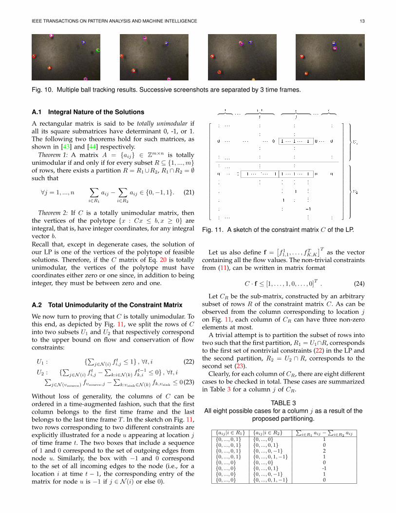
Fig. 10. Multiple ball tracking results. Successive screenshots are separated by 3 time frames.

A.1 Integral Nature of the Solutions

A rectangular matrix is said to be totally unimodular ifall its square submatrices have determinant 0, -1, or 1.The following two theorems hold for such matrices, asshown in [43] and [44] respectively.

Theorem 1: A matrix A = {aij} ∈ Zm×n is totallyunimodular if and only if for every subset R ⊆ {1, ...,m}of rows, there exists a partition R = R1∪R2, R1∩R2 = ∅such that

∀j = 1, ..., n∑i∈R1

aij −∑i∈R2

aij ∈ {0,−1, 1}. (21)

Theorem 2: If C is a totally unimodular matrix, thenthe vertices of the polytope {x : Cx ≤ b, x ≥ 0} areintegral, that is, have integer coordinates, for any integralvector b.Recall that, except in degenerate cases, the solution ofour LP is one of the vertices of the polytope of feasiblesolutions. Therefore, if the C matrix of Eq. 20 is totallyunimodular, the vertices of the polytope must havecoordinates either zero or one since, in addition to beinginteger, they must be between zero and one.

A.2 Total Unimodularity of the Constraint Matrix

We now turn to proving that C is totally unimodular. Tothis end, as depicted by Fig. 11, we split the rows of Cinto two subsets U1 and U2 that respectively correspondto the upper bound on flow and conservation of flowconstraints:

U1 : {∑j∈N (i) f

ti,j ≤ 1} , ∀t, i (22)

U2 : {∑j∈N (i) f

ti,j −

∑k:i∈N (k) f

t−1k,i ≤ 0} , ∀t, i∑

j∈N (υsource)fυsource,j −

∑k:υsink∈N (k) fk,υsink ≤ 0 (23)

Without loss of generality, the columns of C can beordered in a time-augmented fashion, such that the firstcolumn belongs to the first time frame and the lastbelongs to the last time frame T . In the sketch on Fig. 11,two rows corresponding to two different constraints areexplicitly illustrated for a node u appearing at location jof time frame t. The two boxes that include a sequenceof 1 and 0 correspond to the set of outgoing edges fromnode u. Similarly, the box with −1 and 0 correspondto the set of all incoming edges to the node (i.e., for alocation i at time t − 1, the corresponding entry of thematrix for node u is −1 if j ∈ N (i) or else 0).

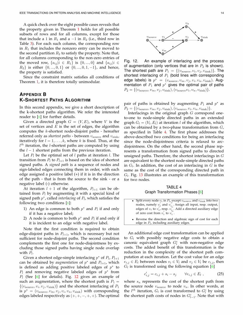
Fig. 11. A sketch of the constraint matrix C of the LP.

Let us also define f =[f11,1, . . . , f

TK,K

]T as the vectorcontaining all the flow values. The non-trivial constraintsfrom (11), can be written in matrix format

C · f ≤ [1, . . . , 1, 0, . . . , 0]T. (24)

Let CR be the sub-matrix, constructed by an arbitrarysubset of rows R of the constraint matrix C. As can beobserved from the column corresponding to location jon Fig. 11, each column of CR can have three non-zeroelements at most.

A trivial attempt is to partition the subset of rows intotwo such that the first partition, R1 = U1∩R, correspondsto the first set of nontrivial constraints (22) in the LP andthe second partition, R2 = U2 ∩ R, corresponds to thesecond set (23).

Clearly, for each column of CR, there are eight differentcases to be checked in total. These cases are summarizedin Table 3 for a column j of CR.

TABLE 3All eight possible cases for a column j as a result of the

proposed partitioning.

{aij |i ∈ R1} {aij |i ∈ R2}∑

i∈R1aij −

∑i∈R2

aij{0, ..., 0, 1} {0, ..., 0} 1{0, ..., 0, 1} {0, ..., 0, 1} 0{0, ..., 0, 1} {0, ..., 0,−1} 2{0, ..., 0, 1} {0, ..., 0, 1,−1} 1{0, ..., 0} {0, ..., 0} 0{0, ..., 0} {0, ..., 0, 1} -1{0, ..., 0} {0, ..., 0,−1} 1{0, ..., 0} {0, ..., 0, 1,−1} 0


A quick check over the eight possible cases reveals thatthe property given in Theorem 1 holds for all possiblesubsets of rows and for all columns, except for thosethat include a 1 in R1 and a −1 in R2 (i.e., third row inTable 3). For each such column, the corresponding rowin R1 that includes the nonzero entry can be moved tothe second partition R2 to satisfy the property. Note that,for all columns corresponding to the non-zero entries ofthe moved row, {aij |i ∈ R1} is {0, ..., 0} and {aij |i ∈R2} is either {0, ..., 0, 1} or {0, ..., 0, 1,−1}, and hence,the property is satisfied.

Since the constraint matrix satisfies all conditions ofTheorem 1, it is therefore totally unimodular.

APPENDIX BK-SHORTEST PATHS ALGORITHM

In this second appendix, we give a short description ofthe k-shortest paths algorithm. We refer the interestedreader to [6] for further details.

Given a directed graph G = (V,E), where V is theset of vertices and E is the set of edges, the algorithmcomputes the k-shortest node-disjoint paths - hereafterreferred only as shortest paths - between υsource and υsink,iteratively for l = 1, . . . , k, where k is fixed. Thus, at thelth iteration, the l-shortest paths are computed by usingthe l − 1 shortest paths from the previous iteration.

Let Pl be the optimal set of l paths at iteration l. Thetransition from Pl to Pl+1 is based on the idea of shortestsigned paths. A signed path is a sequence of nodes andsign-labeled edges connecting them in order, with eachedge assigned a positive label (+) if it is in the directionof the path - that is from the source to the sink - or anegative label (-) otherwise.

At iteration l + 1 of the algorithm, Pl+1 can be ob-tained from Pl by augmenting it with a special kind ofsigned path p∗, called interlacing of Pl, which satisfies thefollowing two conditions [6]:

1) An edge is common to both p∗ and Pl if and onlyif it has a negative label;

2) A node is common to both p∗ and Pl if and only ifit is incident to an edge with negative label.

Note that the first condition is required to obtainedge-disjoint paths in Pl+1, which is necessary but notsufficient for node-disjoint paths. The second conditioncomplements the first one for node-disjointness by ex-cluding those signed paths having single node overlapwith Pl.

Given a shortest edge-simple interlacing p∗ of Pl, Pl+1

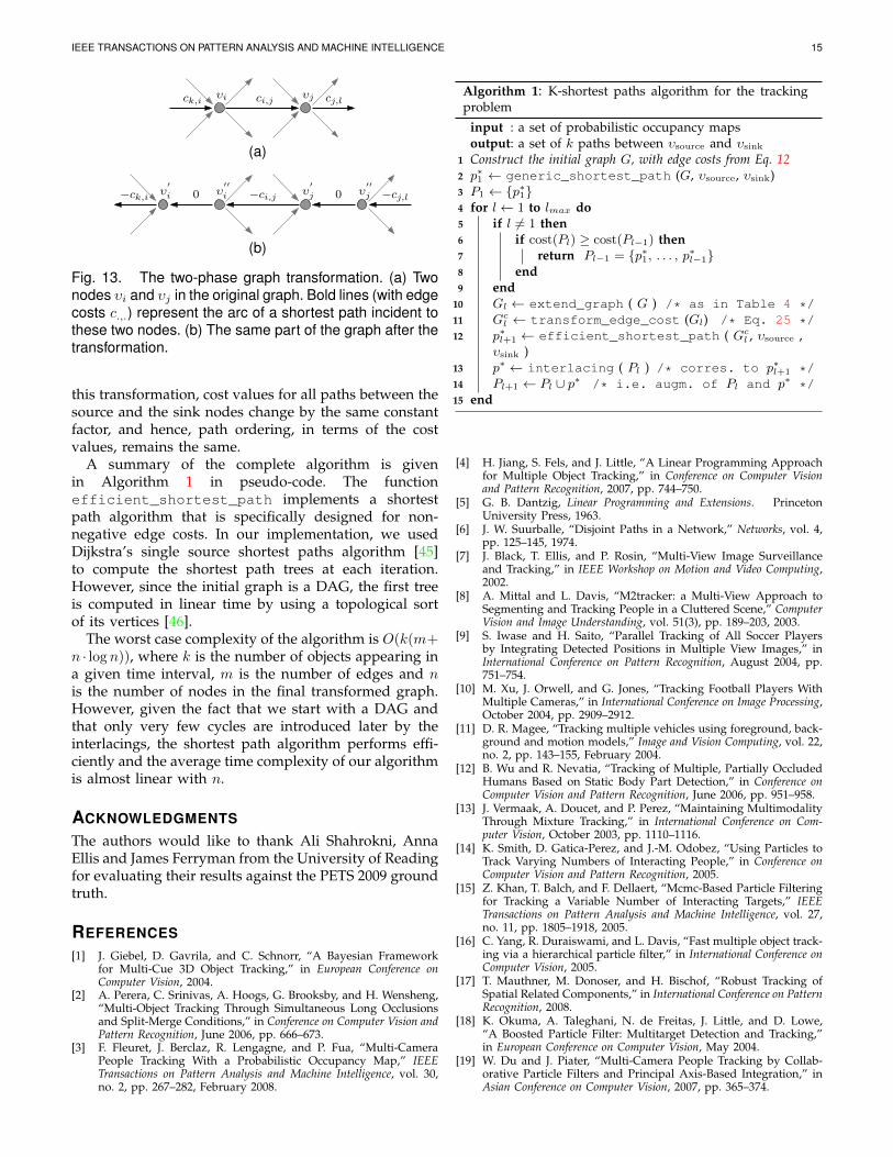
can be obtained by augmentation of p∗ and Pl+1, whichis defined as adding positive labeled edges of p∗ toPl and removing negative labeled edges of p∗ fromPl (See [6] for details). Fig. 12 gives an example ofsuch an augmentation, where the shortest path is P1 ={(υsource, υi, υj , υsink)} and the shortest interlacing of P1

is p∗ = (υsource, υm, υj , υi, υn, υsink) with correspondingedges labeled respectively as (+,+,−,+,+). The optimal

υj

υn

υm

+

+ +

+

υi -υsource υsink

Fig. 12. An example of interlacing and the processof augmentation (only vertices that are in P2 is shown).The shortest path are P1 = {(υsource, υi, υj , υsink)}. Theshortest interlacing of P1 (bold lines with correspondingedge labels) is p∗ = (υsource, υm, υj , υi, υn, υsink). Aug-mentation of P1 and p∗ gives the optimal pair of pathsP2 = {(υsource, υm, υj , υsink), (υsourceυi, υn, υsink)}.

pair of paths is obtained by augmenting P1 and p∗ asP2 = {(υsource, υm, υj , υsink), (υsource, υi, υn, υsink)}.

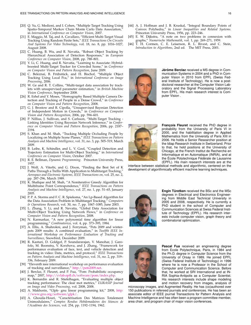
Interlacings in the original graph G correspond one-to-one to node-simple directed paths in an extendedgraph Gl = (Vl, El) at iteration l of the algorithm, whichcan be obtained by a two-phase transformation from G,as specified in Table 4. The first phase addresses theabove-described two conditions for being an interlacingsince the node-disjointness criteria is relaxed to arc-disjointness. On the other hand, the second phase rep-resents a transformation from signed paths to directedunsigned paths. Therefore, the shortest interlacings in Gare equivalent to the shortest node-simple directed pathsin Gl. In addition, the cost of an interlacing in G is thesame as the cost of the corresponding directed path inGl. Fig. 13 illustrates an example of this transformationfor two nodes.

TABLE 4Graph Transformation Phases [6]

• Split every node υi in Pl, except υsource and υsink into twonodes, namely υ

′i and υ

′′i . Assign all input, resp. output,

edges of υi to υ′i , resp. υ

′′i . Add a directed auxiliary edge

of zero cost from υ′i to υ

′′i .

• Reverse the direction and algebraic sign of cost for eachedge in Pl, including auxiliary edges.

An additional edge cost transformation can be appliedto Gl with possibly negative edge costs to obtain acanonic equivalent graph Gcl with non-negative edgecosts. The added benefit of this transformation is thereduction in the complexity of the shortest path com-putation at each iteration. Let the cost value for an edgeei,j ∈ El between nodes vi ∈ Vl and vj ∈ Vl be ci,j , thenGl is transformed using the following equation [6]

c′i,j = ci,j + si − sj ∀ei,j ∈ El , (25)

where sn represents the cost of the shortest path fromthe source node υsource to node vn. In other words, atthe lth iteration, Gl is cost transformed to Gcl by usingthe shortest path costs of nodes in Gcl−1. Note that with


ci,j cj,lck,i υjυi

(a)

υ′i υ

′′i υ

′j υ

′′j −cj,l−ci,j 00−ck,i

(b)

Fig. 13. The two-phase graph transformation. (a) Twonodes υi and υj in the original graph. Bold lines (with edgecosts c.,.) represent the arc of a shortest path incident tothese two nodes. (b) The same part of the graph after thetransformation.

this transformation, cost values for all paths between thesource and the sink nodes change by the same constantfactor, and hence, path ordering, in terms of the costvalues, remains the same.

A summary of the complete algorithm is givenin Algorithm 1 in pseudo-code. The functionefficient_shortest_path implements a shortestpath algorithm that is specifically designed for non-negative edge costs. In our implementation, we usedDijkstra’s single source shortest paths algorithm [45]to compute the shortest path trees at each iteration.However, since the initial graph is a DAG, the first treeis computed in linear time by using a topological sortof its vertices [46].

The worst case complexity of the algorithm is O(k(m+n · log n)), where k is the number of objects appearing ina given time interval, m is the number of edges and nis the number of nodes in the final transformed graph.However, given the fact that we start with a DAG andthat only very few cycles are introduced later by theinterlacings, the shortest path algorithm performs effi-ciently and the average time complexity of our algorithmis almost linear with n.

ACKNOWLEDGMENTS

The authors would like to thank Ali Shahrokni, AnnaEllis and James Ferryman from the University of Readingfor evaluating their results against the PETS 2009 groundtruth.

REFERENCES[1] J. Giebel, D. Gavrila, and C. Schnorr, “A Bayesian Framework

for Multi-Cue 3D Object Tracking,” in European Conference onComputer Vision, 2004.

[2] A. Perera, C. Srinivas, A. Hoogs, G. Brooksby, and H. Wensheng,“Multi-Object Tracking Through Simultaneous Long Occlusionsand Split-Merge Conditions,” in Conference on Computer Vision andPattern Recognition, June 2006, pp. 666–673.

[3] F. Fleuret, J. Berclaz, R. Lengagne, and P. Fua, “Multi-CameraPeople Tracking With a Probabilistic Occupancy Map,” IEEETransactions on Pattern Analysis and Machine Intelligence, vol. 30,no. 2, pp. 267–282, February 2008.

Algorithm 1: K-shortest paths algorithm for the trackingproblem

input : a set of probabilistic occupancy mapsoutput: a set of k paths between υsource and υsinkConstruct the initial graph G, with edge costs from Eq. 121

p∗1 ← generic_shortest_path (G, υsource, υsink)2

P1 ← {p∗1}3

for l← 1 to lmax do4

if l 6= 1 then5

if cost(Pl) ≥ cost(Pl−1) then6

return Pl−1 = {p∗1, . . . , p∗l−1}7

end8

end9

Gl ← extend_graph ( G ) /* as in Table 4 */10

Gcl ← transform_edge_cost (Gl) /* Eq. 25 */11

p∗l+1 ← efficient_shortest_path ( Gcl , υsource ,12

υsink )p∗ ← interlacing ( Pl ) /* corres. to p∗l+1 */13

Pl+1 ← Pl ∪ p∗ /* i.e. augm. of Pl and p∗ */14

end15

[4] H. Jiang, S. Fels, and J. Little, “A Linear Programming Approachfor Multiple Object Tracking,” in Conference on Computer Visionand Pattern Recognition, 2007, pp. 744–750.

[5] G. B. Dantzig, Linear Programming and Extensions. PrincetonUniversity Press, 1963.

[6] J. W. Suurballe, “Disjoint Paths in a Network,” Networks, vol. 4,pp. 125–145, 1974.

[7] J. Black, T. Ellis, and P. Rosin, “Multi-View Image Surveillanceand Tracking,” in IEEE Workshop on Motion and Video Computing,2002.

[8] A. Mittal and L. Davis, “M2tracker: a Multi-View Approach toSegmenting and Tracking People in a Cluttered Scene,” ComputerVision and Image Understanding, vol. 51(3), pp. 189–203, 2003.

[9] S. Iwase and H. Saito, “Parallel Tracking of All Soccer Playersby Integrating Detected Positions in Multiple View Images,” inInternational Conference on Pattern Recognition, August 2004, pp.751–754.

[10] M. Xu, J. Orwell, and G. Jones, “Tracking Football Players WithMultiple Cameras,” in International Conference on Image Processing,October 2004, pp. 2909–2912.

[11] D. R. Magee, “Tracking multiple vehicles using foreground, back-ground and motion models,” Image and Vision Computing, vol. 22,no. 2, pp. 143–155, February 2004.

[12] B. Wu and R. Nevatia, “Tracking of Multiple, Partially OccludedHumans Based on Static Body Part Detection,” in Conference onComputer Vision and Pattern Recognition, June 2006, pp. 951–958.

[13] J. Vermaak, A. Doucet, and P. Perez, “Maintaining MultimodalityThrough Mixture Tracking,” in International Conference on Com-puter Vision, October 2003, pp. 1110–1116.

[14] K. Smith, D. Gatica-Perez, and J.-M. Odobez, “Using Particles toTrack Varying Numbers of Interacting People,” in Conference onComputer Vision and Pattern Recognition, 2005.

[15] Z. Khan, T. Balch, and F. Dellaert, “Mcmc-Based Particle Filteringfor Tracking a Variable Number of Interacting Targets,” IEEETransactions on Pattern Analysis and Machine Intelligence, vol. 27,no. 11, pp. 1805–1918, 2005.

[16] C. Yang, R. Duraiswami, and L. Davis, “Fast multiple object track-ing via a hierarchical particle filter,” in International Conference onComputer Vision, 2005.

[17] T. Mauthner, M. Donoser, and H. Bischof, “Robust Tracking ofSpatial Related Components,” in International Conference on PatternRecognition, 2008.

[18] K. Okuma, A. Taleghani, N. de Freitas, J. Little, and D. Lowe,“A Boosted Particle Filter: Multitarget Detection and Tracking,”in European Conference on Computer Vision, May 2004.

[19] W. Du and J. Piater, “Multi-Camera People Tracking by Collab-orative Particle Filters and Principal Axis-Based Integration,” inAsian Conference on Computer Vision, 2007, pp. 365–374.


[20] Q. Yu, G. Medioni, and I. Cohen, “Multiple Target Tracking UsingSpatio-Temporal Markov Chain Monte Carlo Data Association,”in International Conference on Computer Vision, 2007.

[21] E. Maggio, M. Taj, and A. Cavallaro, “Efficient Multi-Target VisualTracking Using Random Finite Sets,” IEEE Transactions On CircuitsAnd Systems For Video Technology, vol. 18, no. 8, pp. 1016–1027,August 2008.

[22] C. Huang, B. Wu, and R. Nevatia, “Robust Object Tracking byHierarchical Association of Detection Responses,” in EuropeanConference on Computer Vision, 2008, pp. 788–801.

[23] Y. Li, C. Huang, and R. Nevatia, “Learning to Associate: Hybrid-boosted Multi-Target Tracker for Crowded Scene,” in Conferenceon Computer Vision and Pattern Recognition, June 2009.

[24] C. Beleznai, B. Fruhstuck, and H. Bischof, “Multiple ObjectTracking Using Local Pca,” in International Conference on ImageProcessing, 2006.

[25] W. Ge and R. T. Collins, “Multi-target data association by track-lets with unsupervised parameter estimation,” in British MachineVision Conference, September 2008.

[26] R. Eshel and Y. Moses, “Homography Based Multiple Camera De-tection and Tracking of People in a Dense Crowd,” in Conferenceon Computer Vision and Pattern Recognition, 2008.

[27] G. J. Brostow and R. Cipolla, “Unsupervised Bayesian Detectionof Independent Motion in Crowds,” in Conference on ComputerVision and Pattern Recognition, 2006, pp. 594–601.

[28] P. Nillius, J. Sullivan, and S. Carlsson, “Multi-Target Tracking -Linking Identities Using Bayesian Network Inference,” in Confer-ence on Computer Vision and Pattern Recognition, 2006, pp. 2187–2194.

[29] S. Khan and M. Shah, “Tracking Multiple Occluding People byLocalizing on Multiple Scene Planes,” IEEE Transactions on PatternAnalysis and Machine Intelligence, vol. 31, no. 3, pp. 505–519, March2009.

[30] B. Leibe, K. Schindler, and L. V. Gool, “Coupled Detection andTrajectory Estimation for Multi-Object Tracking,” in InternationalConference on Computer Vision, October 2007.

[31] R. E. Bellman, Dynamic Programming. Princeton University Press,1957.

[32] J. Wolf, A. Viterbi, and G. Dixon, “Finding the Best Set of KPaths Through a Trellis With Application to Multitarget Tracking,”Aerospace and Electronic Systems, IEEE Transactions on, vol. 25, no. 2,pp. 287–296, March 1989.

[33] K. Shafique and M. Shah, “A Noniterative Greedy Algorithm forMultiframe Point Correspondence,” IEEE Transactions on PatternAnalysis and Machine Intelligence, vol. 27, no. 1, pp. 51–65, January2005.

[34] P. P. A. Storms and F. C. R. Spieksma, “An Lp-Based Algorithm forthe Data Association Problem in Multitarget Tracking,” Computers& Operations Research, vol. 30, no. 7, pp. 1067–1085, June 2003.

[35] L. Zhang, Y. Li, and R. Nevatia, “Global Data Association forMulti-Object Tracking Using Network Flows,” in Conference onComputer Vision and Pattern Recognition, 2008.

[36] N. Karmarkar, “A new polynomial time algorithm for linearprogramming,” Combinatorica, vol. 4, pp. 373–395, 1984.

[37] A. Ellis, A. Shahrokni, and J. Ferryman, “Pets 2009 and winter-pets 2009 results: A combined evaluation,” in Twelfth IEEE In-ternational Workshop on Performance Evaluation of Tracking andSurveillance, Snowbird, December 2009.

[38] R. Kasturi, D. Goldgof, P. Soundararajan, V. Manohar, J. Garo-folo, M. Boonstra, V. Korzhova, and J. Zhang, “Framework forperformance evaluation of face, text, and vehicle detection andtracking in video: Data, metrics, and protocol,” IEEE Transactionson Pattern Analysis and Machine Intelligence, vol. 31, no. 2, pp. 319–336, February 2009.

[39] “Eleventh ieee international workshop on performance evaluationof tracking and surveillance,” http://pets2009.net.

[40] J. Berclaz, F. Fleuret, and P. Fua, “Pom: Probabilistic occupancymap,” 2007, http://cvlab.epfl.ch/software/pom/index.php.

[41] K. Bernardin and R. Stiefelhagen, “Evaluating multiple objecttracking performance: The clear mot metrics,” EURASIP Journalon Image and Video Processing, vol. 2008, 2008.

[42] A. Makhorin, “Glpk- gnu linear programming kit,” 2008, http://www.gnu.org/software/glpk/.

[43] A. Ghouila-Houri, “Caracterisation Des Matrices TotalementUnimodulaires,” Comptes Rendus Hebdomadaires des Seances del’Academie des Sciences, vol. 254, pp. 1192–1194, 1962.

[44] A. J. Hoffman and J. B. Kruskal, “Integral Boundary Points ofConvex Polyhedra,” in Linear Inequalities and Related Systems.Princeton University Press, 1956, pp. 223–246.

[45] E. W. Dijkstra, “A note on two problems in connexion withgraphs,” Numerische Mathematik, vol. 1, pp. 269–271, 1959.

[46] T. H. Cormen, C. E. Leiserson, R. L. Rivest, and C. Stein,Introduction to Algorithms, 2nd ed. The MIT Press, 2001.

Jerome Berclaz received a MS degree in Com-munication Systems in 2004 and a PhD in Com-puter Vision in 2010 from EPFL (Swiss Fed-eral Institute of Technology). He is now a post-doctoral researcher at the Computer Vision Lab-oratory and the Signal Processing Laboratoryfrom EPFL. His main research interest is Com-puter Vision .

Francois Fleuret received the PhD degree inprobability from the University of Paris VI in2000, and the habilitation degree in AppliedMathematics from the University of Paris XIII in2006. He holds a Senior Researcher position atthe Idiap Research Institute in Switzerland. Priorto that, he held positions at the University ofChicago, at the French Institut de Recherche enInformatique et en Automatique (INRIA), and atthe Ecole Polytechnique Federale de Lausanne(EPFL). His main research interests are at the

interface between statistical methods and algorithmic, centered on thedevelopment of algorithmically efficient machine learning techniques.

Engin Turetken received the BSc and the MScdegrees in Electrical and Electronics Engineer-ing from Middle East Technical University in2005 and 2008, respectively. He is currently aPhD student in the school of Computer andCommunication Sciences at Swiss Federal Insti-tute of Technology (EPFL). His research inter-ests include computer vision, graph theory andcombinatorial optimization.

Pascal Fua received an engineering degreefrom Ecole Polytechnique, Paris, in 1984 andthe Ph.D. degree in Computer Science from theUniversity of Orsay in 1989. He joined EPFL(Swiss Federal Institute of Technology) in 1996where he is now a Professor in the School ofComputer and Communication Science. Beforethat, he worked at SRI International and at IN-RIA Sophia-Antipolis as a Computer Scientist.His research interests include shape modelingand motion recovery from images, analysis of

microscopy images, and Augmented Reality. He has (co)authored over150 publications in refereed journals and conferences. He has been anassociate editor of IEEE journal Transactions for Pattern Analysis andMachine Intelligence and has often been a program committee member,area chair, and program chair of major vision conferences.

http://pets2009.net

http://cvlab.epfl.ch/software/pom/index.php

http://www.gnu.org/software/glpk/

http://www.gnu.org/software/glpk/

Documents

Multiple Object Tracking using K-Shortest Paths Optimization · PDF fileIEEE TRANSACTIONS ON PATTERN ANALYSIS AND MACHINE INTELLIGENCE 1 ... Engin Tˆ uretken, and Pascal Fua,¨ Senior