IEEE TRANSACTIONS ON PATTERN ANALYSIS AND … · problem is solved (the optimization ... APRIL 2011 721. P.F. Felzenszwalb is with the Department ... 0162-8828/11/$26.00 2011 IEEE

Dynamic Programming and Graph Algorithmsin Computer Vision

Pedro F. Felzenszwalb, Member, IEEE Computer Society, and Ramin Zabih, Senior Member, IEEE

Abstract—Optimization is a powerful paradigm for expressing and solving problems in a wide range of areas, and has been

successfully applied to many vision problems. Discrete optimization techniques are especially interesting since, by carefully exploiting

problem structure, they often provide nontrivial guarantees concerning solution quality. In this paper, we review dynamic programming

and graph algorithms, and discuss representative examples of how these discrete optimization techniques have been applied to some

classical vision problems. We focus on the low-level vision problem of stereo, the mid-level problem of interactive object segmentation,

and the high-level problem of model-based recognition.

Index Terms—Combinatorial algorithms, vision and scene understanding, artificial intelligence, computing methodologies.

Ç

1 OPTIMIZATION IN COMPUTER VISION

OPTIMIZATION methods play an important role in compu-ter vision. Vision problems are inherently ambiguous,

and in general, one can only expect to make “educatedguesses” about the content of images. A natural approach toaddress this issue is to devise an objective function thatmeasures the quality of a potential solution and then use anoptimization method to find the best solution. This approachcan often be justified in terms of statistical inference, wherewe look for the hypothesis about the content of an image withthe highest probability of being correct.

It is widely accepted that the optimization framework iswell suited to dealing with noise and other sources ofuncertainty, such as ambiguities in the image data. More-over, by formulating problems in terms of optimization, wecan easily take into account multiple sources of information.Another advantage of the optimization approach is that, inprinciple, it provides a clean separation between how aproblem is formulated (the objective function) and how theproblem is solved (the optimization algorithm). Unfortu-nately, the optimization problems that arise in vision areoften very hard to solve.

In the past decade, there has been a new emphasis ondiscrete optimization methods, such as dynamic program-ming or graph algorithms, for solving computer visionproblems. There are two main differences between discreteoptimization methods and the more classical continuousoptimization approaches commonly used in vision [83].First, of course, these methods work with discrete solutions.Second, discrete methods can often provide nontrivial

guarantees about the quality of the solutions they find.These theoretical guarantees are often accompanied bystrong performance in practice. A good example is theformulation of low-level vision problems, such as stereo,using Markov Random Fields [92], [97] (we will discuss thisin detail in Section 7).

1.1 Overview

This survey covers some of the main discrete optimizationmethods commonly used in computer vision, along with afew selected applications where discrete optimizationmethods have been particularly important. Optimizationis an enormous field, and even within computer vision it isa ubiquitous presence. To provide a coherent narrativerather than an annotated bibliography, our survey isinherently somewhat selective, and there are a number ofrelated topics that we have omitted. We chose to focus ondynamic programming and on graph algorithms since theyshare two key properties: First, they draw on a body of well-established, closely interrelated techniques, which aretypically covered in an undergraduate course on algorithms(using a textbook such [24], [60]), and second, thesemethods have had a significant and increasing impactwithin computer vision over the last decade. Some topicswhich we do not explicitly cover include constrainedoptimization methods (such as linear programming) andmessage passing algorithms (such as belief propagation).

We begin by reviewing some basic concepts of discreteoptimization and introducing some notation. We thensummarize two classical techniques for discrete optimiza-tion, namely, graph algorithms (Section 3) and dynamicprogramming (Section 4); along with each technique, wepresent an example application relevant to computer vision.In Section 5, we describe how discrete optimizationtechniques can be used to perform interactive objectsegmentation. In Section 6, we discuss the role of discreteoptimization for the high-level vision problem of model-based recognition. In Section 7, we focus on the low-levelvision problem of stereo. Finally, in Section 8, we describe afew important recent developments.

IEEE TRANSACTIONS ON PATTERN ANALYSIS AND MACHINE INTELLIGENCE, VOL. 33, NO. 4, APRIL 2011 721

. P.F. Felzenszwalb is with the Department of Computer Science, Universityof Chicago, 1100 E. 58th St., Chicago, IL 60637.E-mail: [email protected].

. R. Zabih is with the Department of Computer Science, Cornell University,4130 Upson Hall, Ithaca, NY 14853. E-mail: [email protected].

Manuscript received 26 Dec. 2008; revised 22 Mar. 2010; accepted 19 May2010; published online 19 July 2010.Recommended for acceptance by D. Kriegman.For information on obtaining reprints of this article, please send e-mail to:[email protected], and reference IEEECS Log NumberTPAMI-2008-12-0884.Digital Object Identifier no. 10.1109/TPAMI.2010.135.

0162-8828/11/$26.00 � 2011 IEEE Published by the IEEE Computer Society

2 DISCRETE OPTIMIZATION CONCEPTS

An optimization problem involves a set of candidatesolutions S and an objective function E : S ! IR thatmeasures the quality of a solution. In general, the searchspace S is defined implicitly and consists of a very largenumber of candidate solutions. The objective function E canmeasure either the goodness or badness of a solution; whenE measures badness, the optimization problem is oftenreferred to as an energy minimization problem and E is calledan energy function. Since many papers in computer visionrefer to optimization as energy minimization, we will followthis convention and assume that an optimal solution x 2 Sis one minimizing an energy function E.

The ideal solution to an optimization problem would bea candidate solution that is a global minimum of the energyfunction, x� ¼ arg minx2SEðxÞ. It is tempting to view theenergy function and the optimization methods as comple-tely independent. This suggests designing an energyfunction that fully captures the constraints of a visionproblem, and then applying a general-purpose energyminimization technique.

However, such an approach fails to pay heed tocomputational issues, which have enormous practicalimportance. No algorithm can find the global minimum ofan arbitrary energy function without exhaustively enumer-ating the search space since any candidate that was notevaluated could turn out to be the best one. As a result, anycompletely general minimization method, such as geneticalgorithms [47] or MCMC [76], is equivalent to exhaustivesearch. On the other hand, it is sometimes possible to designan efficient algorithm that solves problems in a particularclass by exploiting the structure of the search space S andthe energy function E. All of the algorithms described inthis survey are of this nature.

Efficient algorithms for restricted classes of problems canbe very useful since vision problems can often be plausiblyformulated in several different ways. One of these problemformulations, in turn, might admit an efficient algorithm,which would make this formulation preferable. A naturalexample which we will discuss in Section 7 comes frompixel labeling problems such as stereo.

Note that, in general, a global minimum of an energyfunction might not give the best results in terms ofaccuracy because the energy function might not capturethe right constraints. But if we use an energy minimizationalgorithm that provides no theoretical guarantees, it can bedifficult to decide if poor performance is due to the choiceof energy function as opposed to weaknesses in theminimization algorithm.

There is a long history of formulating pixel labelingproblems in terms of optimization, and some very complexand elegant energy functions have been proposed (see [41]for some early examples). Yet the experimental perfor-mance of these methods was poor since they relied ongeneral-purpose optimization techniques such as simulatedannealing [6], [41]. In the last decade, researchers havedeveloped efficient discrete algorithms for a relativelysimple class of energy functions, and these optimization-based schemes are viewed as the state of the art for stereo[21], [92].

2.1 Common Classes of Energy Functions in Vision

As mentioned before, the problems that arise in computervision are inevitably ambiguous, with multiple candidatesolutions that are consistent with the observed data. Inorder to eliminate ambiguities, it is usually necessary tointroduce a bias toward certain candidate solutions. Thereare many ways to describe and justify such a bias. In thecontext of statistical inference, the bias is usually called aprior. We will use this term informally to refer to any termsin an energy function that impose such a bias.

Formulating a computer vision problem in terms ofoptimization often makes the prior clear. Most of the energyfunctions that are used in vision have a general form thatreflects the observed data and the need for a prior:

EðxÞ ¼ EdataðxÞ þ EpriorðxÞ: ð1Þ

The first term of such an energy function penalizescandidate solutions that are inconsistent with the observeddata, while the second term imposes the prior.

We will often consider an n-dimensional search space ofthe form S ¼ Ln, where L is an arbitrary finite set. We willrefer to L as a set of labels, and will use k to denote the sizeof L. This search space has an exponential number, kn, ofpossible solutions. A candidate solution x 2 Ln will bewritten as ðx1; . . . ; xnÞ, where xi 2 L. We will also considersearch spaces S ¼ L1 � � � � � Ln, which simply allows theuse of a different label set for each xi.

A particularly common class of energy functions incomputer vision can be written as

Eðx1; . . . ; xnÞ ¼X

i

DiðxiÞ þX

i;j

Vi;jðxi; xjÞ: ð2Þ

Many of the energy functions we will consider will be ofthis form. In general, the terms Di are used to ensure thatthe label xi is consistent with the image data, while the Vi;jterms ensure that the labels xi and xj are compatible.

Energy functions of the form given in (2) have a longhistory in computer vision. They are particularly commonin pixel labeling problems, where a candidate solutionassigns a label to each pixel in the image, and the priorcaptures a spatial smoothness assumption.

For these low-level vision problems, the labels mightrepresent quantities such as stereo depth (see Section 7),intensity, motion, texture, etc. In all of these problems, theunderlying data are ambiguous, and if each pixel is viewedin isolation, it is unclear what the correct label should be.

One approach to deal with the ambiguity at each pixel isto examine the data at nearby pixels to choose its label. If thelabels are intensities, this often corresponds to a simplefiltering algorithm (e.g., convolution with a Gaussian). Forstereo or motion, such algorithms are usually referred to asarea-based; a relatively early example is provided in [46].Unfortunately, these methods have severe problems nearobject boundaries since the majority of pixels near a pixel pmay not support the correct label for p. This shows up in thevery poor performance of area-based methods on thestandard stereo benchmarks [92].

Optimization provides a natural way to address pixellabeling problems. The use of optimization for such aproblem appears to date to the groundbreaking work of

722 IEEE TRANSACTIONS ON PATTERN ANALYSIS AND MACHINE INTELLIGENCE, VOL. 33, NO. 4, APRIL 2011

Horn and Schunk [48] on motion. They proposed a contin-uous energy function, where a data term measures howconsistent the candidate labeling is with the observations ateach pixel, and a prior ensures the smoothness of the solution.Note that their prior preferred labelings that are globallysmooth; this caused motion boundaries to be oversmoothed,which is a very important issue in pixel labeling problems.The energy minimization problem was solved by a contin-uous technique, namely, the calculus of variations.

Following [48], many energy functions were proposed,both for motion and for other pixel labeling problems. Aninteresting snapshot of the field is provided by Poggio et al.[82], who point out the ties between the smoothness termused by the authors of [48] and the use of Tikhonovregularization to solve inverse problems [98]. Anotherimportant development was [41], which showed that suchenergy functions have a natural statistical interpretation asmaximizing the posterior probability of a Markov RandomField (MRF). This paper was so influential that to this day,many authors use the terminology of MRF to describe anoptimization approach to pixel labeling problems (see [18],[52], [63], [97] for a few examples).

A very different application of energy functions of theform in (2) involves object recognition and matching withdeformable models. One of the earliest examples is thepictorial structures formulation for part-based modeling in[36]. In this case, we have an object with many parts and asolution corresponds to an assignment of image locations toeach part. In the energy function from [36], a data termmeasures how much the image data under each part agreewith a model of the part’s appearance, and the priorenforces geometrical constraints between different pairs ofparts. A related application involves boundary detectionusing active contour models [3], [56]. In this case, the dataterm measures the evidence for a boundary at a particularlocation in the image, and the prior enforces smoothness ofthe boundary. Discrete optimization methods are quiteeffective both for pictorial structures (see Section 6.3) andactive contour models (Section 5.2).

The optimization approach for object detection andrecognition makes it possible to combine different sourcesof information (such as the appearance of parts and theirgeometric arrangement) into a single objective function. Inthe case of part-based modeling, this makes it possible toaggregate information from different parts without relyingon a binary decision coming from an individual partdetector. The formulation can also be understood in termsof statistical estimation, where the most probable objectconfiguration is found [34].

2.2 Guarantees Concerning Solution Quality

One of the most important properties of discrete optimiza-tion methods is that they often provide some kind ofguarantee concerning the quality of the solutions they find.Ideally, the algorithm can be shown to compute the globalminimum of the energy function. While we will discuss anumber of methods that can do this, many of theoptimization problems that arise in vision are NP-hard(see [20, Appendix] for an important example). Instead,many algorithms look for a local minimum—a candidatethat is better than all “nearby” alternatives. A general view

of a local minimum, which we take from [2], is to define aneighborhood system N : S ! 2S that specifies, for anycandidate solution x, the set of nearby candidates NðxÞ.Using this notation, a local minimum solution with respectto the neighborhood system N is a candidate x� such thatEðx�Þ � minx2Nðx�ÞEðxÞ.

In computer vision, it is common to deal with energyfunctions with multiple local minima. Problems with asingle minimum can often be addressed via the large bodyof work in convex optimization (see [13] for a recenttextbook). Note that for some optimization problems, if wepick the neighborhood system N carefully, a local minimumis also a global minimum.

A local minimum is usually computed by an iterativeprocess where an initial candidate is improved by explicitlyor implicitly searching the neighborhood of nearby solu-tions. This subproblem of finding the best solution withinthe local neighborhood is quite important. If we have a fastalgorithm for finding the best nearby solution within a largeneighborhood, we can perform this local improvement steprepeatedly.1 There are a number of important visionapplications where such an iterated local improvementmethod has been employed. For example, object segmenta-tion via active contour models [56] can be performed in thisway, where the local improvement step uses dynamicprogramming [3] (see Section 5.2 for details). Similarly, low-level vision problems such as stereo can be solved by usingmin-cut algorithms in the local improvement step [20] (seeSection 7).

While proving that an algorithm converges to a stronglocal minimum is important, this does not directly implythat the solution is close to optimal. In contrast, anapproximation algorithm for an optimization problem is apolynomial-time algorithm that computes a solution xwhose energy is within a multiplicative factor of the globalminimum. It is generally quite difficult to prove such abound, and approximation algorithms are a major researcharea in theoretical computer science (see [60] for aparticularly clear exposition of the topic). Very fewapproximation algorithms have been developed in compu-ter vision; the best known is the expansion move algorithmof [20]. An alternative approach is to provide per-instancebounds, where the algorithm produces a guarantee that thesolution is within some factor of the global minimum, butwhere that factor varies with each problem instance.

The fundamental difference between continuous anddiscrete optimization methods concerns the nature of thesearch space. In a continuous optimization problem, we areusually looking for a set of real numbers and the number ofcandidate solutions is uncountable; in a discrete optimiza-tion problem, we are looking for an element from a discrete(and, often, finite) set. Note that there is ongoing work (e.g.,[14]) that explores the relationship between continuous anddiscrete optimization methods for vision.

While continuous methods are quite powerful, it isuncommon for them to produce guarantees concerning theabsolute quality of the solutions they find (unless, of course,

FELZENSZWALB AND ZABIH: DYNAMIC PROGRAMMING AND GRAPH ALGORITHMS IN COMPUTER VISION 723

1. Ahuja et al. [2] refer to such algorithms as very large-scaleneighborhood search techniques; in vision, they are sometimes calledmove-making algorithms [71].

the energy function is convex). Instead, they tend to provideguarantees about speed of convergence toward a localminimum. Whether or not guarantees concerning solutionquality are important depends on the particular problem andcontext. Moreover, despite their lack of such guarantees,continuous methods can perform quite well in practice.

2.3 Relaxations

The complexity of minimizing a particular energy functionclearly depends on the set it is being minimized over, but theform of this dependence can be counterintuitive. Inparticular, sometimes it is difficult to minimize E over theoriginal discrete set S, but easy to minimize E over acontinuous set S0 that contains S. Minimizing E over S0instead of S is called a relaxation of the original problem. Ifthe solution to the relaxation (i.e., the global minimum of Eover S0) happens to occur at an element of S, then by solvingthe relaxation, we have solved the original problem. As ageneral rule, however, if the solution to the relaxation doesnot lie in S, it provides no information about the originalproblem beyond a lower bound (since there can be no bettersolution within S than the best solution in the larger set S0).In computer vision, the most widely used relaxationsinvolve linear programming or spectral graph partitioning.

Linear programming provides an efficient way to mini-mize a linear objective function subject to linear inequalityconstraints (which define a polyhedral region). One of thebest known theorems concerning linear programming is thatwhen an optimal solution exists, it can be achieved at a vertexof the polyhedral region defined by the inequality constraints(see, e.g., [23]). A linear program can thus be viewed as adiscrete optimization problem over the vertices of a poly-hedron. Yet, linear programming has some unusual featuresthat distinguish it from the methods that we survey. Forexample, linear programming can provide a per-instancebound (see [67] for a nice application in low-level vision).Linear programming is also the basis for many approxima-tion algorithms [60]. There is also a rich mathematical theorysurrounding linear programs, including linear programmingduality, which plays an important role in advancedoptimization methods that don’t explicitly use linearprogramming algorithms.

Linear programming has been used within vision for anumber of problems, and one recent application that hasreceived significant interest involves message passingmethods. The convergence of belief propagation on theloopy graphs common in vision is not well understood, butseveral recent papers [101], [102] have exposed strongconnections with linear programming.

Spectral partitioning methods can efficiently cluster thevertices of a graph by computing a specific eigenvector ofan associated matrix (see, e.g., [54]). These methods areexemplified by the well-known normalized cut algorithm incomputer vision [96]. Typically, a discrete objective functionis first written down, which is NP-hard to optimize. Withcareful use of spectral graph partitioning, a relaxation of theproblem can be solved efficiently. Currently, there is notechnique that converts a solution to the relaxation into asolution to the original discrete problem that is provablyclose to the global minimum. However, these methods canstill perform well in practice.

2.4 Problem Reductions

A powerful technique which we will use throughout thissurvey paper is the classical computer science notion of aproblem reduction [38]. In a problem reduction, we showhow an algorithm that solves one problem can also be usedto solve a different problem, usually by transforming anarbitrary instance of the second problem to an instance ofthe first.2

There are two ways that problem reductions are useful.Suppose that the second problem is known to be difficult(for example, it may be NP-hard, and hence, widelybelieved to require exponential time). In this case, theproblem reduction gives a proof that the first problem is atleast as difficult as the second. However, discrete optimiza-tion methods typically perform a reduction in the oppositedirection by reducing a difficult-appearing problem to onethat can be solved quickly. This is the focus of our survey.

One immediate issue with optimization is that it is almost“too powerful” a paradigm. Many NP-hard problems fallwithin the realm of discrete optimization. On the other hand,problems with easy solutions can also be phrased in terms ofoptimization; for example, consider the problem of sortingn numbers. The search space consists of the set ofn! permutations, and the objective function might count thenumber of pairs that are misordered. As the example ofsorting should make clear, expressing a problem in terms ofoptimization can sometimes obscure the solution.

Since the optimization paradigm is so general, we shouldnot expect to find a single algorithm that works well on mostoptimization problems. This leads to the perhaps counter-intuitive notion that to solve any specific problem, it isusually preferable to use the most specialized technique thatcan be applied. This ensures that we exploit the structure ofthe specific problem to the greatest extent possible.

3 GRAPH ALGORITHMS

Many discrete optimization methods have a natural inter-pretation in terms of a graph G ¼ ðV; EÞ, given by a set ofvertices V and a set of edges E (vertices are sometimescalled nodes and edges are sometimes called links). In adirected graph, each edge e is an ordered pair of verticese ¼ ðu; vÞ, while in an undirected graph, the vertices in anedge e ¼ fu; vg are unordered. We will often associate anonnegative weight we to each edge e in a graph. We saythat two vertices are neighbors if they are connected by anedge. In computer vision, the vertices V usually correspondto pixels or features such as interest points extracted froman image, while the edges E encode spatial relationships.

A path from a vertex u to a vertex v is a sequence ofdistinct vertices starting at u and ending at v such that forany two consecutive vertices, a and b, in the sequence eitherða; bÞ 2 E or fa; bg 2 E depending on whether or not thegraph is directed. The length of a path in a weighted graphis the sum of the weights associated with the edgesconnecting consecutive vertices in the path. A cycle isdefined like a path except that the first and last vertices inthe sequence are the same. We say that a graph is acyclic if


2. We will only consider reductions that do not significantly increase thesize of the problem (see [38] for more discussion of this issue).

it has no cycles. An undirected graph is connected if there isa path between any two vertices in V. A tree is a connectedacyclic undirected graph.

Now consider a directed graph with two distinguishedvertices s and t called the terminals. An s� t cut is apartition of the vertices into two components S and T suchthat s 2 S and t 2 T .3 The cost of the cut is the sum of theweights on edges going from vertices in S to vertices in T .

A matching M in an undirected graph is a subset of theedges such that each vertex is in at most one edge in M. Aperfect matching is one where every vertex is in some edgein M. The weight of a matching M in a weighted graph isthe sum of the weights associated with edges in M. We saythat a graph is bipartite if the vertices can be partitionedinto two sets A and B such that every edge connects avertex in A to a vertex in B. A perfect matching in abipartite graph defines a one-to-one correspondence be-tween vertices in A and vertices in B.

3.1 Shortest Path Algorithms

The shortest paths problem involves finding minimumlength paths between pairs of vertices in a graph. Theproblem has many important applications and it is also usedas a subroutine to solve a variety of other optimizationproblems (such as computing minimum cuts). There are twocommon versions of the problem: 1) In the single-source case,we want to find a shortest path from a source vertex s toevery other vertex in a graph; 2) in the all-pairs case, we lookfor a shortest path between every pair of vertices in a graph.Here, we mainly consider the single-source case as this is theone most often used in computer vision. We discuss itsapplication to interactive segmentation in Section 5.1. Wenote that, in general, solving the single-source shortest pathsproblem is not actually harder than computing a shortestpath between a single pair of vertices.

The main property that we can use to efficiently computeshortest paths is that they have an optimal substructureproperty: A subpath of a shortest path is itself a shortestpath. All of the shortest paths algorithms use this fact.

The most well-known algorithm for the single-sourceshortest paths problem is due to Dijkstra [31]. For a directedgraph, Dijkstra’s algorithm can be implemented to run inOðjVj2Þ or OðjEj log jVjÞ time, assuming that there is at leastone edge touching each node in the graph. The algorithmassumes that all edge weights are nonnegative and buildsshortest paths from a source in order of increasing length.

Dijkstra’s algorithm assumes that all edge weights arenonnegative. In fact, computing shortest paths on anarbitrary graph with negative edge weights is NP-hard(since this would allow us to find Hamiltonian paths [68]).However, there is an algorithm that can handle graphs withsome negative edge weights as long as there are no negativelength cycles. The Bellman-Ford algorithm [24] can be usedto solve the single-source problem on such graphs inOðjEjjVjÞ time. The method is based on dynamic program-ming (see Section 4). It sequentially computes shortest pathsthat use at most i edges in order of increasing i. TheBellman-Ford algorithm can also be used to detect negative

length cycles on arbitrary graphs. This is an importantsubroutine for computing minimum ratio cycles and hasbeen applied to image segmentation [53] and deformableshape matching [93].

The all-pairs shortest paths problem can be solved usingmultiple calls to Dijkstra’s algorithm. We can simply solvethe single-source problem starting at every possible node inthe graph. This leads to an overall method that runs inOðjEjjVj log jVjÞ time. This is a good approach to solve theall-pairs shortest paths problem in sparse graphs. If thegraph is dense, we are better off using the Floyd-Warshallalgorithm. That algorithm is based on dynamic program-ming and runs in OðjVj3Þ time. Moreover, like the Bellman-Ford algorithm, it can be used as long as there are nonegative length cycles in the graph. Another advantage ofthe Floyd-Warshall method is that it can be implemented injust a few lines of code and does not rely on an efficientpriority queue data structure (see [24]).

3.2 Minimum Cut Algorithms

The minimum cut problem (“min-cut”) is to find theminimum cost s� t cut in a directed graph. On the surface,this problem may look intractable. In fact, many variationson the problem, such as requiring that more than twoterminals be separated, are NP-hard [28].

It is possible to show that there is a polynomial-timealgorithm to compute the min-cut, by relying on resultsfrom submodular function optimization. Given a set U anda function f defined on all subsets of U, consider therelationship between fðAÞ þ fðBÞ and fðA \BÞ þ fðA [BÞ.If the two quantities are equal (such as when f is setcardinality), the function f is said to be modular. IffðAÞ þ fðBÞ � fðA \BÞ þ fðA [BÞ, f is said to be sub-modular. Submodular functions can be minimized in high-order polynomial time [91], and have recently foundimportant applications in machine vision [64], [66] as wellas areas such as spatial statistics [69].

There is a close relationship between submodularfunctions and graph cuts (see, e.g., [27]). Given a graph,let U be the nodes of the graph and fðAÞ be the sum of theweights of the edges from nodes in A to nodes not in A.Such an f is called a cut function, and the followingargument shows it to be submodular. Each term in fðA \BÞ þ fðA [BÞ also appears in fðAÞ þ fðBÞ. Now consideran edge that starts at a node that is in A, but not in B, andends at a node in B, but not in A. Such an edge appears infðAÞ þ fðBÞ but not in fðA \BÞ þ fðA [BÞ. Thus, a cutfunction f is not modular. A very similar argument showsthat the cost of an s� t cut is also a submodular function:U consists of the nonterminal nodes and fðAÞ is theweight of the outgoing edges from A [ fsg, which is thecost of the cut.

While cut functions are submodular, the class ofsubmodular functions is much more general. As we havepointed out, this suggests that special-purpose min-cutalgorithms would be preferable to general-purpose sub-modular function minimization techniques [91] (which, infact, are not yet practical for large problems). In fact, thereare very efficient min-cut algorithms.

The key to computing min-cuts efficiently is the famousproblem reduction of Ford and Fulkerson [37]. The reduction


3. There is also an equivalent definition of a cut as a set of edges, whichsome authors use [14], [20].

uses the maximum flow problem (“max-flow”), which isdefined on the same directed graph, but the edge weights arenow interpreted as capacity constraints. An s� t flow is anassignment of nonnegative values to the edges in thegraph where the value of each edge is no more than itscapacity. Furthermore, at every nonterminal vertex, thesum of values assigned to incoming edges equals the sumof values assigned to outgoing edges.

Informally speaking, most max-flow algorithms repeat-edly find a path between s and t with spare capacity, andthen increase (augment) the flow along this path. For aparticularly clear explanation of max-flow and its relation-ship to min-cut, see [60]. From the standpoint of computervision, max-flow algorithms are very fast and can even beused for real-time systems (see, e.g., [65]). In fact, most ofthe graphs that arise in vision are largely grids, like theexample shown in Fig. 1. These graphs have many shortpaths from s to t, which, in turn, suggests the use of max-flow algorithms that are specially designed for visionproblems, such as [16].

3.3 Example Application: Binary Image Restorationvia Graph Cuts

There are a number of algorithms for solving low-levelvision problems that compute a minimum s� t cut on anappropriately defined graph. This technique is usuallycalled “graph cuts” (the term appears to originate in [19]).4

The idea has been applied to a number of problems incomputer vision, medical imaging, and computer graphics(see [17] for a recent survey). We will describe the use ofgraph cuts for interactive object segmentation in Section 5.3and for stereo in Section 7.1. However, their originalapplication to vision was for binary image restoration [42].

Consider a binary image where each pixel has beenindependently corrupted (for example, the output of anerror-prone document scanner). Our goal is to clean up theimage. This can be naturally formulated as an optimizationproblem of the form defined by (2). The labels are binary, sothe search space is f0; 1gn, where n is the number of pixels inthe image and there are 2n possible solutions. The functionDi

provides a cost for labeling the ith pixel using one of twopossible values; in practice, this cost would be zero for it tohave the same label that was observed in the corrupted

image, and a positive constant � for it to have the oppositelabel. The simplest choice for Vi;jðxi; xjÞ is a 0-1 valuedfunction, which is 1 just in case pixels i and j are adjacent andxi 6¼ xj. Putting these together, we see that Eðx1 . . . ; xnÞequals � times the number of pixels that get assigned a valuedifferent from the one observed in the corrupted image, plusthe number of adjacent pixels with different labels. Byminimizing this energy, we find a spatially coherent labelingthat is similar to the observed data.

This energy function is often referred to as the Isingmodel (its generalization to more than two labels is calledthe Potts model). Greig et al. [42] showed that the problemof minimizing this energy can be reduced to the min-cutproblem on an appropriately constructed graph.5 The graphis shown in Fig. 1 for a 9-pixel image. In this graph, theterminals s; t correspond to the labels 0 and 1. Besides theterminals, there is one vertex per pixel; each such pixelvertex is connected to the adjacent pixel vertices and to eachterminal vertex. A cut in this graph leaves each pixel vertexconnected to exactly one terminal vertex. This naturallycorresponds to a binary labeling. With the appropriatechoice of edge weights, the cost of a cut is the energy of thecorresponding labeling.6 The weight of edges cut betweenpixel vertices will add to the number of adjacent pixels withdifferent labels; the weight of edges cut between pixelvertices and terminals will sum to � times the number ofpixels with labels that differ from those values observed inthe input data.

It is important to realize that this construction dependson the specific form of the Ising model energy function.Since the terminals in the graph correspond to the labels,the construction is restricted to two labels. As mentionedabove, the natural multiterminal variants of the min-cutproblem are NP-hard [28]. In addition, we cannot expect tobe able to efficiently solve even simple generalizations ofthe Ising energy-energy function since minimizing the Pottsenergy function with three labels is NP-hard [20].

3.4 Bipartite Matching Algorithms

In the minimum weight bipartite matching problem, wehave a bipartite graph with V ¼ A [B and weights weassociated with each edge. The goal is to find a perfectmatching M with minimum total weight. Perfect matchingsin bipartite graphs are particularly interesting because theyrepresent one-to-one correspondences between elements inA and elements in B. In computer vision, the problem offinding correspondences between two sets of elements hasmany applications, ranging from three-dimensional recon-struction [30] to object recognition [9].

The bipartite matching problem described here is alsoknown as the assignment problem. We also note that there is aversion of the problem that involves finding a maximumweight matching in a bipartite graph, without requiring thatthe matching be perfect. That problem is essentially


Fig. 1. Cuts separating the terminals (labeled 0 and 1) in this graphcorrespond to binary labelings of a 3� 3 image. The dark nodes are thepixel vertices. This graph assumes the usual 4-connected neighborhoodsystem among pixels.

4. Despite the similar names, graph cuts are not closely related tonormalized cuts.

5. As [66] points out, the actual construction dates back at least 40 years,but [42] first applied it to images.

6. There are two ways to encode the correspondence between cuts andlabelings. If pixel p gets labeled 0, this can be encoded by cutting the edgebetween the vertex for p and the terminal vertex for 0, or to leaving thisedge intact (and thus, cutting the edge to the terminal vertex for 1). Thedifferent encodings lead to slightly different weights for the edges betweenterminals and pixels.

equivalent to the one described here (they can be reduced toeach other) [68].

We can solve the bipartite matching problem inOðn3Þ timeusing the Hungarian algorithm [80], where n ¼ jAj ¼ jBj.That algorithm relies on linear programming duality and therelationship between matchings and vertex covers tosequentially solve a set of intermediate problems, eventuallyleading to a solution of the original matching problem.

One practical algorithm for bipartite matching relies onthe following generalization of the maximum flow problem.Let G be a directed graph with a capacity ce and weight weassociated with each edge e 2 E. Let s and t be two terminalnodes (the source and the sink) and let f be an s� t flowwith value fðeÞ on edge e. The cost of the flow is defined asP

e2EðfðeÞ � weÞ. In the minimum cost flow problem, we fix avalue for the flow and search for a flow of that value withminimum cost. This problem can be solved using anapproach similar to the Ford-Fulkerson method for theclassical max-flow problem by sequentially finding aug-menting paths in a weighted residual graph. When thecapacities are integral, this approach is guaranteed to find aminimum cost flow with integer values in each edge.

The bipartite matching problem on a graph can bereduced to a minimum cost flow problem. We simply directthe edges in E so they go from A to B, and add two nodes sand t such that there is an edge of weight zero from s toevery node in A and to t from every node in B. Thecapacities are all set to one. An integer flow of value n in themodified graph (n ¼ jAj ¼ jBjÞ corresponds to a perfectmatching in the original graph, and the cost of the flow isthe weight of the matching.

4 DYNAMIC PROGRAMMING

Dynamic programming [8] is a powerful general techniquefor developing efficient discrete optimization algorithms. Incomputer vision, it has been used to solve a variety ofproblems, including curve detection [3], [39], [77], contourcompletion [95], stereo matching [5], [79], and deformableobject matching [4], [7], [25], [34], [32].

The basic idea of dynamic programming is to decomposea problem into a set of subproblems such that 1) given asolution to the subproblems, we can quickly compute asolution to the original problem and 2) the subproblems canbe efficiently solved recursively in terms of each other. Animportant aspect of dynamic programming is that thesolution of a single subproblem is often used multiple timesfor solving several larger subproblems. Thus, in a dynamicprogramming algorithm, we need to “cache” solutions toavoid recomputing them later on. This is what makesdynamic programming algorithms different from classicalrecursive methods.

Similarly to the shortest paths algorithms, dynamicprogramming relies on an optimal substructure property.This makes it possible to solve a subproblem usingsolutions of smaller subproblems.

In practice, we can think of a dynamic programmingalgorithm as a method for filling in a table, where each tableentry corresponds to one of the subproblems we need tosolve. The dynamic programming algorithm iterates overtable entries and computes a value for the current entryusing values of entries that it has already computed. Often,

there is a simple recursive equation which defines the valueof an entry in terms of values of other entries, butsometimes determining a value involves a more complexcomputation.

4.1 Dynamic Programming on a Sequence

Suppose that we have a sequence of n elements and wewant to assign a label from L to each element in thesequence. In this case, we have a search space S ¼ Ln,where a candidate solution ðx1; . . . ; xnÞ assigns label xi tothe ith element of the sequence. A natural energy functionfor sequence labeling can be defined as follows: Let DiðxiÞbe a cost for assigning the label xi to the ith element of thesequence. Let V ðxi; xiþ1Þ be a cost for assigning twoparticular labels to a pair of neighboring elements. Nowthe cost of a candidate solution can be defined as

Eðx1; . . . ; xnÞ ¼Xn

i¼1

DiðxiÞ þXn�1

i¼1

V ðxi; xiþ1Þ: ð3Þ

This objective function measures the cost of assigning alabel to each element and penalizes “incompatible” assign-ments between neighboring elements. Usually, Di is used tocapture a cost per element that depends on some input data,while V encodes a prior that is fixed over all inputs.Optimization problems of this form are common in anumber of vision applications, including in some formula-tions of the stereo problem, as discussed in Section 7.2, andin visual tracking [29]. The MAP estimation problem for ageneral hidden Markov model [84] also leads to anoptimization problem of this form.

Now we show how to use dynamic programming toquickly compute a solution ðx�1; . . . ; x�nÞ minimizing anenergy function of the form in (3). The algorithm worksfilling in tables storing costs of optimal partial solutions ofincreasing size. Let Bi½xi� denote the cost of the bestassignment of labels to the first i elements in the sequencewith the constraint that the ith element has the label xi.These are the “subproblems” used by the dynamicprogramming procedure. We can fill in the tables Bi inorder of increasing i using the recursive equations:

B1½x1� ¼ D1ðx1Þ; ð4Þ

Bi½xi� ¼ DiðxiÞ þminxi�1

Bi�1½xi�1� þ V ðxi�1; xiÞð Þ: ð5Þ

Once the Bi are computed, the optimal solution to theoverall problem can be obtained by taking x�n ¼arg minxnBn½xn� and tracing back, in order of decreasing i:

x�i ¼ arg minxi

Bi½xi� þ V ðxi; x�iþ1Þ� �

: ð6Þ

Another common approach for tracing back the optimalsolution involves caching the optimal ði� 1Þth label as afunction of the ith label in a separate table whencomputing Bi:

Ti½xi� ¼ arg minxi�1

Bi�1½xi�1� þ V ðxi�1; xiÞð Þ: ð7Þ

Then, after we compute x�n, we can track back by takingx�i�1 ¼ Ti½x�i � starting at i ¼ n. This simplifies the tracing backprocedure at the expense of a higher memory requirement.


The dynamic programming algorithm runs in Oðnk2Þtime. The running time is dominated by the computation ofthe tables Bi. There are OðnÞ tables to be filled in, each tablehas OðkÞ entries, and it takes OðkÞ time to fill in one tableentry using the recursive equation (5).

In many important cases, the dynamic programmingsolution described here can be sped up using the distancetransform methods in [33]. In particular, in many situations(including the signal restoration application describedbelow), L is a subset of IR and the pairwise cost is of theform V ðxi; xjÞ ¼ jxi � xjjp or V ðxi; xjÞ ¼ minðjxi � xjjp; �Þfor some p > 1 and � > 0. In this case, the distancetransform methods can be used to compute all entries inBi (after Bi�1 is computed) in OðkÞ time. This leads to anoverall algorithm that runs in OðnkÞ time, which is optimalassuming that the input is given by an arbitrary set ofnk costs DiðxiÞ. In this case, any algorithm would have tolook at each of those costs, which takes at least OðnkÞ time.

4.2 Relationship to Shortest Paths

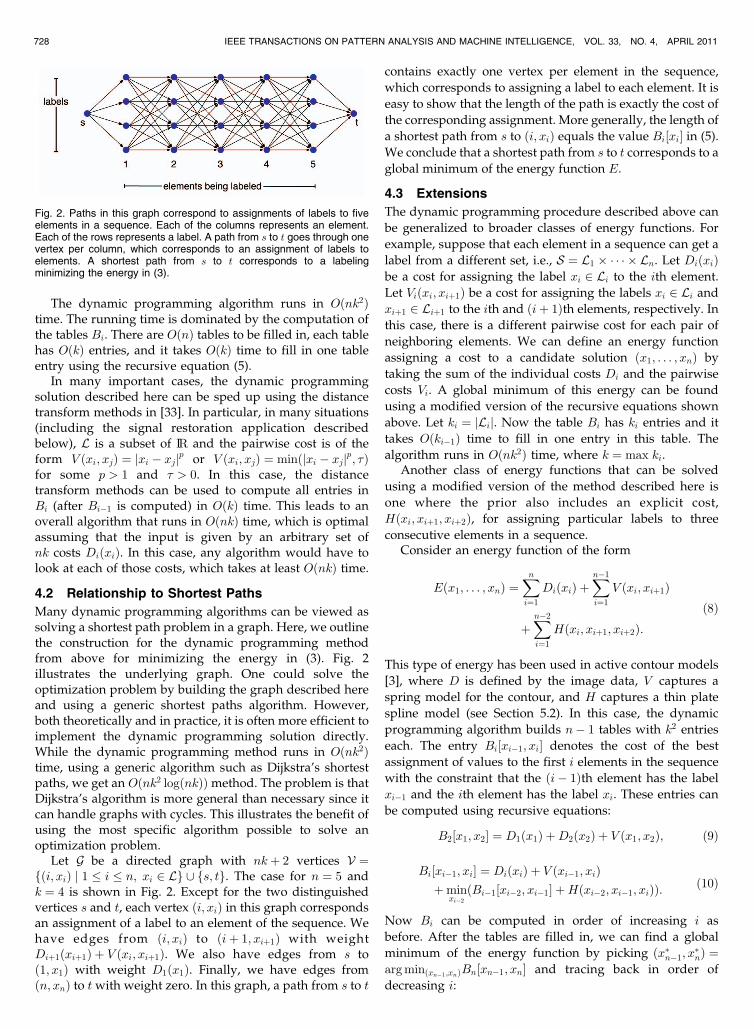
Many dynamic programming algorithms can be viewed assolving a shortest path problem in a graph. Here, we outlinethe construction for the dynamic programming methodfrom above for minimizing the energy in (3). Fig. 2illustrates the underlying graph. One could solve theoptimization problem by building the graph described hereand using a generic shortest paths algorithm. However,both theoretically and in practice, it is often more efficient toimplement the dynamic programming solution directly.While the dynamic programming method runs in Oðnk2Þtime, using a generic algorithm such as Dijkstra’s shortestpaths, we get an Oðnk2 logðnkÞÞmethod. The problem is thatDijkstra’s algorithm is more general than necessary since itcan handle graphs with cycles. This illustrates the benefit ofusing the most specific algorithm possible to solve anoptimization problem.

Let G be a directed graph with nkþ 2 vertices V ¼fði; xiÞ j 1 � i � n; xi 2 Lg [ fs; tg. The case for n ¼ 5 andk ¼ 4 is shown in Fig. 2. Except for the two distinguishedvertices s and t, each vertex ði; xiÞ in this graph correspondsan assignment of a label to an element of the sequence. Wehave edges from ði; xiÞ to ðiþ 1; xiþ1Þ with weightDiþ1ðxiþ1Þ þ V ðxi; xiþ1Þ. We also have edges from s toð1; x1Þ with weight D1ðx1Þ. Finally, we have edges fromðn; xnÞ to t with weight zero. In this graph, a path from s to t

contains exactly one vertex per element in the sequence,

which corresponds to assigning a label to each element. It is

easy to show that the length of the path is exactly the cost of

the corresponding assignment. More generally, the length of

a shortest path from s to ði; xiÞ equals the value Bi½xi� in (5).

We conclude that a shortest path from s to t corresponds to a

global minimum of the energy function E.

4.3 Extensions

The dynamic programming procedure described above can

be generalized to broader classes of energy functions. For

example, suppose that each element in a sequence can get a

label from a different set, i.e., S ¼ L1 � � � � � Ln. Let DiðxiÞbe a cost for assigning the label xi 2 Li to the ith element.

Let Viðxi; xiþ1Þ be a cost for assigning the labels xi 2 Li and

xiþ1 2 Liþ1 to the ith and ðiþ 1Þth elements, respectively. In

this case, there is a different pairwise cost for each pair of

neighboring elements. We can define an energy function

assigning a cost to a candidate solution ðx1; . . . ; xnÞ by

taking the sum of the individual costs Di and the pairwise

costs Vi. A global minimum of this energy can be found

using a modified version of the recursive equations shown

above. Let ki ¼ jLij. Now the table Bi has ki entries and it

takes Oðki�1Þ time to fill in one entry in this table. The

algorithm runs in Oðnk2Þ time, where k ¼ max ki.Another class of energy functions that can be solved

using a modified version of the method described here is

one where the prior also includes an explicit cost,

Hðxi; xiþ1; xiþ2Þ, for assigning particular labels to three

consecutive elements in a sequence.Consider an energy function of the form

Eðx1; . . . ; xnÞ ¼Xn

i¼1

DiðxiÞ þXn�1

i¼1

V ðxi; xiþ1Þ

þXn�2

i¼1

Hðxi; xiþ1; xiþ2Þ:ð8Þ

This type of energy has been used in active contour models

[3], where D is defined by the image data, V captures a

spring model for the contour, and H captures a thin plate

spline model (see Section 5.2). In this case, the dynamic

programming algorithm builds n� 1 tables with k2 entries

each. The entry Bi½xi�1; xi� denotes the cost of the best

assignment of values to the first i elements in the sequence

with the constraint that the ði� 1Þth element has the label

xi�1 and the ith element has the label xi. These entries can

be computed using recursive equations:

B2½x1; x2� ¼ D1ðx1Þ þD2ðx2Þ þ V ðx1; x2Þ; ð9Þ

Bi½xi�1; xi� ¼ DiðxiÞ þ V ðxi�1; xiÞþmin

xi�2

ðBi�1½xi�2; xi�1� þHðxi�2; xi�1; xiÞÞ: ð10Þ

Now Bi can be computed in order of increasing i as

before. After the tables are filled in, we can find a global

minimum of the energy function by picking ðx�n�1; x�nÞ ¼

arg minðxn�1;xnÞBn½xn�1; xn� and tracing back in order of

decreasing i:


Fig. 2. Paths in this graph correspond to assignments of labels to fiveelements in a sequence. Each of the columns represents an element.Each of the rows represents a label. A path from s to t goes through onevertex per column, which corresponds to an assignment of labels toelements. A shortest path from s to t corresponds to a labelingminimizing the energy in (3).

x�i ¼ argminxi

Biþ1½xi; x�iþ1� þHðxi; x�iþ1; x�iþ2Þ

� �:

This method takes Oðnk3Þ time. In general, we can minimizeenergy functions that explicitly take into account the labelsof m consecutive elements in OðnkmÞ time.

4.4 Example Application: 1D Signal Restoration viaDynamic Programming

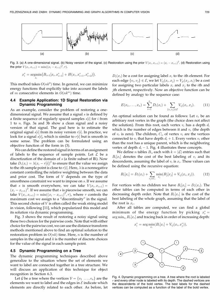
As an example, consider the problem of restoring a one-dimensional signal. We assume that a signal s is defined bya finite sequence of regularly spaced samples s½i� for i from1 to n. Figs. 3a and 3b show a clean signal and a noisyversion of that signal. The goal here is to estimate theoriginal signal s½i� from its noisy version r½i�. In practice, welook for a signal s½i�, which is similar to r½i� but is smooth insome sense. The problem can be formulated using anobjective function of the form in (3).

We can define the restored signal in terms of an assignmentof labels to the sequence of sample points. Let L be adiscretization of the domain of s (a finite subset of IR). Nowtake DiðxiÞ ¼ �ðxi � r½i�Þ2 to ensure that the value we assignto the ith sample point is close to r½i�. Here, � is a nonnegativeconstant controlling the relative weighting between the dataand prior cost. The form of V depends on the type ofsmoothness constraint we want to impose on s. If we assumethat s is smooth everywhere, we can take V ðxi; xiþ1Þ ¼ðxi � xiþ1Þ2. If we assume that s is piecewise smooth, we cantake V ðxi; xiþ1Þ ¼ minððxi � xiþ1Þ2; �Þ, where � controls themaximum cost we assign to a “discontinuity” in the signal.This second choice of V is often called the weak string modelin vision, following [11], which popularized this model andits solution via dynamic programming.

Fig. 3 shows the result of restoring a noisy signal usingthese two choices for the pairwise costs. Note that with eitherchoice for the pairwise cost, we can use the distance transformmethods mentioned above to find an optimal solution to therestoration problem in OðnkÞ time. Here, n is the number ofsamples in the signal and k is the number of discrete choicesfor the value of the signal in each sample point.

4.5 Dynamic Programming on a Tree

The dynamic programming techniques described abovegeneralize to the situation where the set of elements wewant to label are connected together in a tree structure. Wewill discuss an application of this technique for objectrecognition in Section 6.3.

Let G be a tree where the vertices V ¼ fv1 . . . ; vng are theelements we want to label and the edges in E indicate whichelements are directly related to each other. As before, let

DiðxiÞ be a cost for assigning label xi to the ith element. For

each edge fvi; vjg 2 E, we let Vijðxi; xjÞ ¼ Vjiðxj; xiÞ be a cost

for assigning two particular labels xi and xj to the ith and

jth element, respectively. Now an objective function can be

defined by analogy to the sequence case:

Eðx1; . . . ; xnÞ ¼Xn

i¼1

DiðxiÞ þX

fvi;vjg2EVijðxi; xjÞ: ð11Þ

An optimal solution can be found as follows: Let vr be anarbitrary root vertex in the graph (the choice does not affectthe solution). From this root, each vertex vi has a depth diwhich is the number of edges between it and vr (the depthof vr is zero). The children, Ci, of vertex vi are the verticesconnected to vi that have depth di þ 1. Every vertex vi otherthan the root has a unique parent, which is the neighboringvertex of depth di � 1. Fig. 4 illustrates these concepts.

We define n tables Bi, each with k ¼ jLj entries such that

Bi½xi� denotes the cost of the best labeling of vi and its

descendents, assuming the label of vi is xi. These values can

be defined using the recursive equation:

Bi½xi� ¼ DiðxiÞ þX

vj2CiminxjðBj½xj� þ Vijðxi; xjÞÞ: ð12Þ

For vertices with no children we have Bi½xi� ¼ DiðxiÞ. Theother tables can be computed in terms of each other indecreasing depth order. Note that Br½xr� is the cost of thebest labeling of the whole graph, assuming that the label ofthe root is xr.

After all tables are computed, we can find a global

minimum of the energy function by picking x�r ¼arg minxrBr½xr� and tracing back in order of increasing depth:

x�i ¼ arg minxiðBi½xi� þ Vijðxi; x�j ÞÞ;


Fig. 3. (a) A one-dimensional signal. (b) Noisy version of the signal. (c) Restoration using the prior V ðxi; xiþ1Þ ¼ ðxi � xiþ1Þ2. (d) Restoration using

the prior V ðxi; xiþ1Þ ¼ minððxi � xiþ1Þ2; �Þ.

Fig. 4. Dynamic programming on a tree. A tree where the root is labeledr and every other node is labeled with its depth. The dashed vertices arethe descendents of the bold vertex. The best labels for the dashedvertices can be computed as a function of the label of the bold vertex.

where vj is the parent of vi. The overall algorithm runs inOðnk2Þ time. As in the case for sequences, distance transformtechniques can often be used to obtain an OðnkÞ timealgorithm [34]. This speedup is particularly important forthe pictorial structure matching problem discussed inSection 6.3. In that problem, k is on the order of the numberof pixels in an image and a quadratic algorithm is notpractical.

We note that dynamic programming can also be used tominimize energy functions defined over certain graphs withcycles [4], [32]. Although the resulting algorithms are lessefficient, they still run in polynomial time. Their asymptoticrunning time depends exponentially on a measure of graphconnectivity called treewidth; trees have treewidth 1, while asquare grid with n nodes has treewidth Oð ffiffiffinp Þ. In manycases, including the case of tree discussed here, the problemcannot usually be solved via shortest paths algorithmsbecause there is no way to encode the cost of a solution interms of the length of a path in a reasonably sized graph.However, a generalization of Dijkstra’s shortest pathsalgorithm to such cases was first proposed in [61] and morerecently explored in [35].

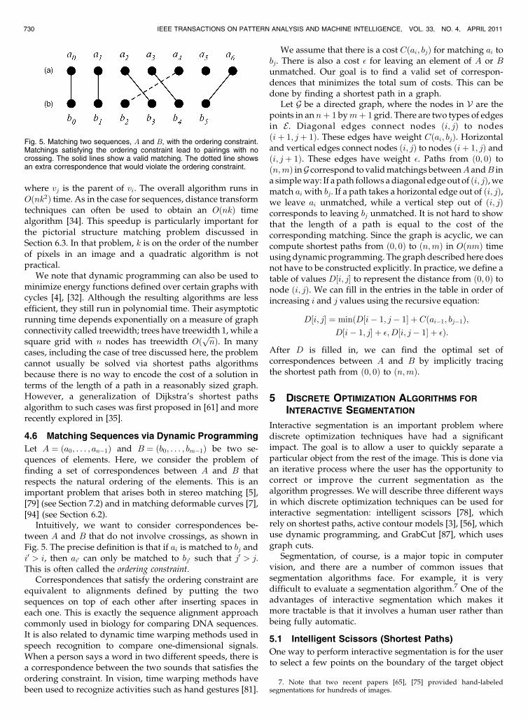
4.6 Matching Sequences via Dynamic Programming

Let A ¼ ða0; . . . ; an�1Þ and B ¼ ðb0; . . . ; bm�1Þ be two se-quences of elements. Here, we consider the problem offinding a set of correspondences between A and B thatrespects the natural ordering of the elements. This is animportant problem that arises both in stereo matching [5],[79] (see Section 7.2) and in matching deformable curves [7],[94] (see Section 6.2).

Intuitively, we want to consider correspondences be-tween A and B that do not involve crossings, as shown inFig. 5. The precise definition is that if ai is matched to bj andi0 > i, then ai0 can only be matched to bj0 such that j0 > j.This is often called the ordering constraint.

Correspondences that satisfy the ordering constraint areequivalent to alignments defined by putting the twosequences on top of each other after inserting spaces ineach one. This is exactly the sequence alignment approachcommonly used in biology for comparing DNA sequences.It is also related to dynamic time warping methods used inspeech recognition to compare one-dimensional signals.When a person says a word in two different speeds, there isa correspondence between the two sounds that satisfies theordering constraint. In vision, time warping methods havebeen used to recognize activities such as hand gestures [81].

We assume that there is a cost Cðai; bjÞ for matching ai tobj. There is also a cost � for leaving an element of A or Bunmatched. Our goal is to find a valid set of correspon-dences that minimizes the total sum of costs. This can bedone by finding a shortest path in a graph.

Let G be a directed graph, where the nodes in V are thepoints in an nþ 1 bymþ 1 grid. There are two types of edgesin E. Diagonal edges connect nodes ði; jÞ to nodesðiþ 1; jþ 1Þ. These edges have weight Cðai; bjÞ. Horizontaland vertical edges connect nodes ði; jÞ to nodes ðiþ 1; jÞ andði; jþ 1Þ. These edges have weight �. Paths from ð0; 0Þ toðn;mÞ inG correspond to valid matchings betweenA andB ina simple way: If a path follows a diagonal edge out of ði; jÞ, wematch ai with bj. If a path takes a horizontal edge out of ði; jÞ,we leave ai unmatched, while a vertical step out of ði; jÞcorresponds to leaving bj unmatched. It is not hard to showthat the length of a path is equal to the cost of thecorresponding matching. Since the graph is acyclic, we cancompute shortest paths from ð0; 0Þ to ðn;mÞ in OðnmÞ timeusing dynamic programming. The graph described here doesnot have to be constructed explicitly. In practice, we define atable of values D½i; j� to represent the distance from ð0; 0Þ tonode ði; jÞ. We can fill in the entries in the table in order ofincreasing i and j values using the recursive equation:

D½i; j� ¼ minðD½i� 1; j� 1� þ Cðai�1; bj�1Þ;D½i� 1; j� þ �;D½i; j� 1� þ �Þ:

After D is filled in, we can find the optimal set ofcorrespondences between A and B by implicitly tracingthe shortest path from ð0; 0Þ to ðn;mÞ.

5 DISCRETE OPTIMIZATION ALGORITHMS FOR

INTERACTIVE SEGMENTATION

Interactive segmentation is an important problem wherediscrete optimization techniques have had a significantimpact. The goal is to allow a user to quickly separate aparticular object from the rest of the image. This is done viaan iterative process where the user has the opportunity tocorrect or improve the current segmentation as thealgorithm progresses. We will describe three different waysin which discrete optimization techniques can be used forinteractive segmentation: intelligent scissors [78], whichrely on shortest paths, active contour models [3], [56], whichuse dynamic programming, and GrabCut [87], which usesgraph cuts.

Segmentation, of course, is a major topic in computervision, and there are a number of common issues thatsegmentation algorithms face. For example, it is verydifficult to evaluate a segmentation algorithm.7 One of theadvantages of interactive segmentation which makes itmore tractable is that it involves a human user rather thanbeing fully automatic.

5.1 Intelligent Scissors (Shortest Paths)

One way to perform interactive segmentation is for the userto select a few points on the boundary of the target object


Fig. 5. Matching two sequences, A and B, with the ordering constraint.Matchings satisfying the ordering constraint lead to pairings with nocrossing. The solid lines show a valid matching. The dotted line showsan extra correspondence that would violate the ordering constraint.

7. Note that two recent papers [65], [75] provided hand-labeledsegmentations for hundreds of images.

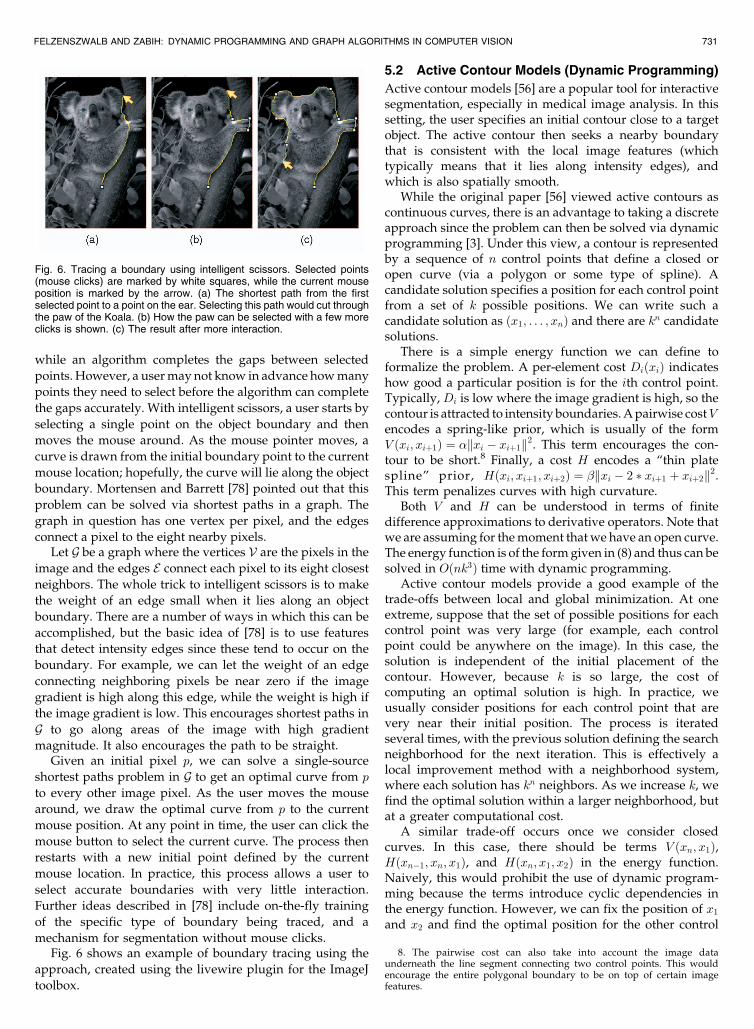
while an algorithm completes the gaps between selected

points. However, a user may not know in advance how many

points they need to select before the algorithm can complete

the gaps accurately. With intelligent scissors, a user starts by

selecting a single point on the object boundary and then

moves the mouse around. As the mouse pointer moves, a

curve is drawn from the initial boundary point to the current

mouse location; hopefully, the curve will lie along the object

boundary. Mortensen and Barrett [78] pointed out that this

problem can be solved via shortest paths in a graph. The

graph in question has one vertex per pixel, and the edges

connect a pixel to the eight nearby pixels.Let G be a graph where the vertices V are the pixels in the

image and the edges E connect each pixel to its eight closest

neighbors. The whole trick to intelligent scissors is to make

the weight of an edge small when it lies along an object

boundary. There are a number of ways in which this can be

accomplished, but the basic idea of [78] is to use features

that detect intensity edges since these tend to occur on the

boundary. For example, we can let the weight of an edge

connecting neighboring pixels be near zero if the image

gradient is high along this edge, while the weight is high if

the image gradient is low. This encourages shortest paths in

G to go along areas of the image with high gradient

magnitude. It also encourages the path to be straight.Given an initial pixel p, we can solve a single-source

shortest paths problem in G to get an optimal curve from p

to every other image pixel. As the user moves the mouse

around, we draw the optimal curve from p to the current

mouse position. At any point in time, the user can click the

mouse button to select the current curve. The process then

restarts with a new initial point defined by the current

mouse location. In practice, this process allows a user to

select accurate boundaries with very little interaction.

Further ideas described in [78] include on-the-fly training

of the specific type of boundary being traced, and a

mechanism for segmentation without mouse clicks.Fig. 6 shows an example of boundary tracing using the

approach, created using the livewire plugin for the ImageJ

toolbox.

5.2 Active Contour Models (Dynamic Programming)

Active contour models [56] are a popular tool for interactivesegmentation, especially in medical image analysis. In thissetting, the user specifies an initial contour close to a targetobject. The active contour then seeks a nearby boundarythat is consistent with the local image features (whichtypically means that it lies along intensity edges), andwhich is also spatially smooth.

While the original paper [56] viewed active contours ascontinuous curves, there is an advantage to taking a discreteapproach since the problem can then be solved via dynamicprogramming [3]. Under this view, a contour is representedby a sequence of n control points that define a closed oropen curve (via a polygon or some type of spline). Acandidate solution specifies a position for each control pointfrom a set of k possible positions. We can write such acandidate solution as ðx1; . . . ; xnÞ and there are kn candidatesolutions.

There is a simple energy function we can define toformalize the problem. A per-element cost DiðxiÞ indicateshow good a particular position is for the ith control point.Typically, Di is low where the image gradient is high, so thecontour is attracted to intensity boundaries. A pairwise costVencodes a spring-like prior, which is usually of the formV ðxi; xiþ1Þ ¼ �kxi � xiþ1k2. This term encourages the con-tour to be short.8 Finally, a cost H encodes a “thin platespline” prior, Hðxi; xiþ1; xiþ2Þ ¼ �kxi � 2 � xiþ1 þ xiþ2k2.This term penalizes curves with high curvature.

Both V and H can be understood in terms of finitedifference approximations to derivative operators. Note thatwe are assuming for the moment that we have an open curve.The energy function is of the form given in (8) and thus can besolved in Oðnk3Þ time with dynamic programming.

Active contour models provide a good example of thetrade-offs between local and global minimization. At oneextreme, suppose that the set of possible positions for eachcontrol point was very large (for example, each controlpoint could be anywhere on the image). In this case, thesolution is independent of the initial placement of thecontour. However, because k is so large, the cost ofcomputing an optimal solution is high. In practice, weusually consider positions for each control point that arevery near their initial position. The process is iteratedseveral times, with the previous solution defining the searchneighborhood for the next iteration. This is effectively alocal improvement method with a neighborhood system,where each solution has kn neighbors. As we increase k, wefind the optimal solution within a larger neighborhood, butat a greater computational cost.

A similar trade-off occurs once we consider closedcurves. In this case, there should be terms V ðxn; x1Þ,Hðxn�1; xn; x1Þ, and Hðxn; x1; x2Þ in the energy function.Naively, this would prohibit the use of dynamic program-ming because the terms introduce cyclic dependencies inthe energy function. However, we can fix the position of x1

and x2 and find the optimal position for the other control


Fig. 6. Tracing a boundary using intelligent scissors. Selected points(mouse clicks) are marked by white squares, while the current mouseposition is marked by the arrow. (a) The shortest path from the firstselected point to a point on the ear. Selecting this path would cut throughthe paw of the Koala. (b) How the paw can be selected with a few moreclicks is shown. (c) The result after more interaction.

8. The pairwise cost can also take into account the image dataunderneath the line segment connecting two control points. This wouldencourage the entire polygonal boundary to be on top of certain imagefeatures.

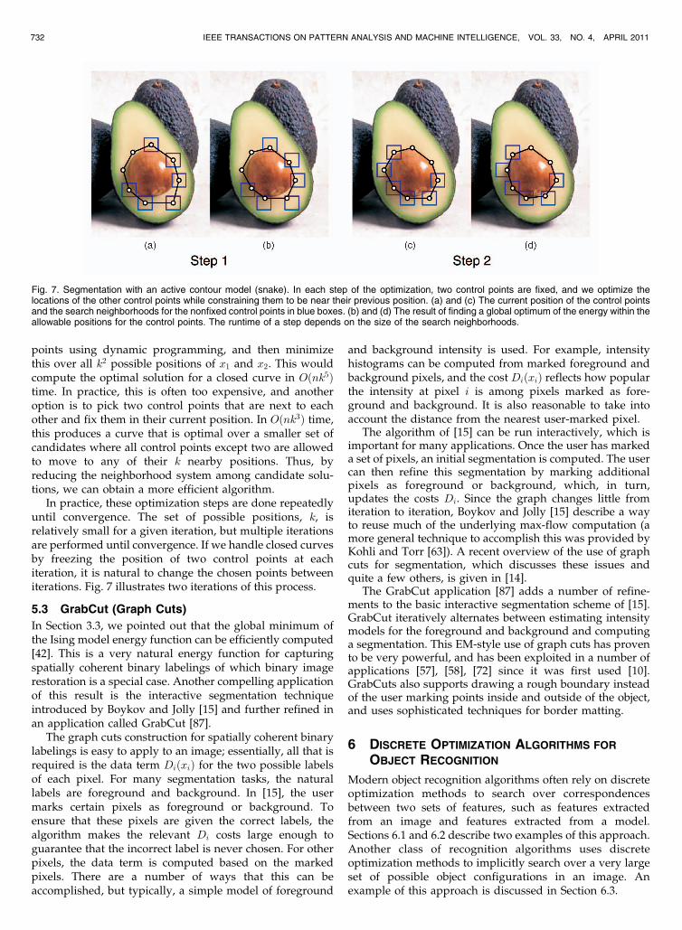
points using dynamic programming, and then minimizethis over all k2 possible positions of x1 and x2. This wouldcompute the optimal solution for a closed curve in Oðnk5Þtime. In practice, this is often too expensive, and anotheroption is to pick two control points that are next to eachother and fix them in their current position. In Oðnk3Þ time,this produces a curve that is optimal over a smaller set ofcandidates where all control points except two are allowedto move to any of their k nearby positions. Thus, byreducing the neighborhood system among candidate solu-tions, we can obtain a more efficient algorithm.

In practice, these optimization steps are done repeatedlyuntil convergence. The set of possible positions, k, isrelatively small for a given iteration, but multiple iterationsare performed until convergence. If we handle closed curvesby freezing the position of two control points at eachiteration, it is natural to change the chosen points betweeniterations. Fig. 7 illustrates two iterations of this process.

5.3 GrabCut (Graph Cuts)

In Section 3.3, we pointed out that the global minimum ofthe Ising model energy function can be efficiently computed[42]. This is a very natural energy function for capturingspatially coherent binary labelings of which binary imagerestoration is a special case. Another compelling applicationof this result is the interactive segmentation techniqueintroduced by Boykov and Jolly [15] and further refined inan application called GrabCut [87].

The graph cuts construction for spatially coherent binarylabelings is easy to apply to an image; essentially, all that isrequired is the data term DiðxiÞ for the two possible labelsof each pixel. For many segmentation tasks, the naturallabels are foreground and background. In [15], the usermarks certain pixels as foreground or background. Toensure that these pixels are given the correct labels, thealgorithm makes the relevant Di costs large enough toguarantee that the incorrect label is never chosen. For otherpixels, the data term is computed based on the markedpixels. There are a number of ways that this can beaccomplished, but typically, a simple model of foreground

and background intensity is used. For example, intensityhistograms can be computed from marked foreground andbackground pixels, and the cost DiðxiÞ reflects how popularthe intensity at pixel i is among pixels marked as fore-ground and background. It is also reasonable to take intoaccount the distance from the nearest user-marked pixel.

The algorithm of [15] can be run interactively, which isimportant for many applications. Once the user has markeda set of pixels, an initial segmentation is computed. The usercan then refine this segmentation by marking additionalpixels as foreground or background, which, in turn,updates the costs Di. Since the graph changes little fromiteration to iteration, Boykov and Jolly [15] describe a wayto reuse much of the underlying max-flow computation (amore general technique to accomplish this was provided byKohli and Torr [63]). A recent overview of the use of graphcuts for segmentation, which discusses these issues andquite a few others, is given in [14].

The GrabCut application [87] adds a number of refine-ments to the basic interactive segmentation scheme of [15].GrabCut iteratively alternates between estimating intensitymodels for the foreground and background and computinga segmentation. This EM-style use of graph cuts has provento be very powerful, and has been exploited in a number ofapplications [57], [58], [72] since it was first used [10].GrabCuts also supports drawing a rough boundary insteadof the user marking points inside and outside of the object,and uses sophisticated techniques for border matting.


OBJECT RECOGNITION

Modern object recognition algorithms often rely on discreteoptimization methods to search over correspondencesbetween two sets of features, such as features extractedfrom an image and features extracted from a model.Sections 6.1 and 6.2 describe two examples of this approach.Another class of recognition algorithms uses discreteoptimization methods to implicitly search over a very largeset of possible object configurations in an image. Anexample of this approach is discussed in Section 6.3.


Fig. 7. Segmentation with an active contour model (snake). In each step of the optimization, two control points are fixed, and we optimize thelocations of the other control points while constraining them to be near their previous position. (a) and (c) The current position of the control pointsand the search neighborhoods for the nonfixed control points in blue boxes. (b) and (d) The result of finding a global optimum of the energy within theallowable positions for the control points. The runtime of a step depends on the size of the search neighborhoods.

6.1 Recognition Using Shape Contexts(Bipartite Matching)

Belongie et al. [9] described a method for comparing edgemaps (or binary images) which has been used in a variety ofapplications. The approach is based on a three-stageprocess: 1) A set of correspondences is found between thepoints in two edge maps, 2) the correspondences are used toestimate a nonlinear transformation aligning the edge maps,and 3) a similarity measure between the two edge maps iscomputed which takes into account both the similaritybetween corresponding points and the amount of deforma-tion introduced by the aligning transformation.

Let A and B be two edge maps. In the first stage of theprocess, we want to find a mapping � : A! B putting eachpoint in A in correspondence to its “best” matching point inB. For each pair of points pi 2 A and pj 2 B, a cost Cðpi; pjÞfor mapping pi to pj is defined, which takes into account thegeometric distribution of edge points around pi and pj. Thiscost is based on a local descriptor called the shape context ofa point. The descriptor is carefully constructed so that it isinvariant to translations and fairly insensitive to smalldeformations. Fig. 8 illustrates two points on differentshapes with similar shape contexts.

Given the set of matching costs between pairs of pointsin A and B, we can look for a map � minimizing the totalcost, Hð�Þ ¼

Ppi2A Cðpi; �ðpiÞÞ, subject to the constraint that

� is one-to-one and onto. This is precisely the weightedbipartite matching problem from Section 3.4. To solve theproblem, we build a bipartite graph G ¼ ðV; EÞ such thatV ¼ A [B and there is an edge between each vertex pi in Aand each vertex pj in B with weight Cðpi; pjÞ. Perfectmatchings in this graph correspond to valid maps � and theweight of the matching is exactly the total cost of the map.

To handle outliers and to find correspondences betweenedge maps with different numbers of points, we can add“dummy” vertices to each side of the bipartite graph toobtain a new set of vertices V0 ¼ A0 [B0. We connect adummy vertex in one side of the graph to each nondummyvertex in the other side using edges with a fixed positiveweight, while dummy vertices are connected to each otherby edges of weight zero. Whenever a point in one edge maphas no good correspondence in the other edge map, it willbe matched to a dummy vertex. This is interpreted asleaving the point unmatched. The number of dummyvertices in each side is chosen so that jA0j ¼ jB0j. This

ensures that the graph has a perfect matching. In the casewhere A and B have different sizes, some vertices in thelarger set will always be matched to dummy vertices.

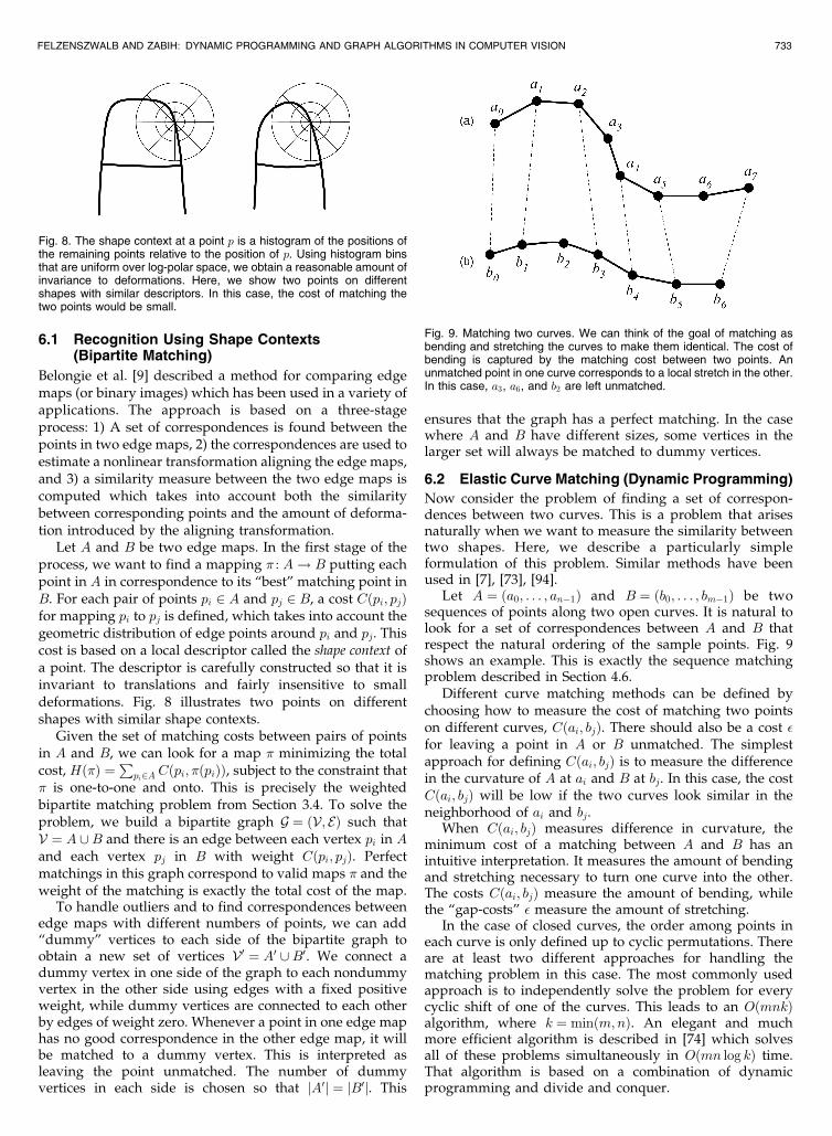
6.2 Elastic Curve Matching (Dynamic Programming)

Now consider the problem of finding a set of correspon-dences between two curves. This is a problem that arisesnaturally when we want to measure the similarity betweentwo shapes. Here, we describe a particularly simpleformulation of this problem. Similar methods have beenused in [7], [73], [94].

Let A ¼ ða0; . . . ; an�1Þ and B ¼ ðb0; . . . ; bm�1Þ be twosequences of points along two open curves. It is natural tolook for a set of correspondences between A and B thatrespect the natural ordering of the sample points. Fig. 9shows an example. This is exactly the sequence matchingproblem described in Section 4.6.

Different curve matching methods can be defined bychoosing how to measure the cost of matching two pointson different curves, Cðai; bjÞ. There should also be a cost �for leaving a point in A or B unmatched. The simplestapproach for defining Cðai; bjÞ is to measure the differencein the curvature of A at ai and B at bj. In this case, the costCðai; bjÞ will be low if the two curves look similar in theneighborhood of ai and bj.

When Cðai; bjÞ measures difference in curvature, theminimum cost of a matching between A and B has anintuitive interpretation. It measures the amount of bendingand stretching necessary to turn one curve into the other.The costs Cðai; bjÞ measure the amount of bending, whilethe “gap-costs” � measure the amount of stretching.

In the case of closed curves, the order among points ineach curve is only defined up to cyclic permutations. Thereare at least two different approaches for handling thematching problem in this case. The most commonly usedapproach is to independently solve the problem for everycyclic shift of one of the curves. This leads to an OðmnkÞalgorithm, where k ¼ minðm;nÞ. An elegant and muchmore efficient algorithm is described in [74] which solvesall of these problems simultaneously in Oðmn log kÞ time.That algorithm is based on a combination of dynamicprogramming and divide and conquer.


Fig. 8. The shape context at a point p is a histogram of the positions ofthe remaining points relative to the position of p. Using histogram binsthat are uniform over log-polar space, we obtain a reasonable amount ofinvariance to deformations. Here, we show two points on differentshapes with similar descriptors. In this case, the cost of matching thetwo points would be small.

Fig. 9. Matching two curves. We can think of the goal of matching asbending and stretching the curves to make them identical. The cost ofbending is captured by the matching cost between two points. Anunmatched point in one curve corresponds to a local stretch in the other.In this case, a3, a6, and b2 are left unmatched.

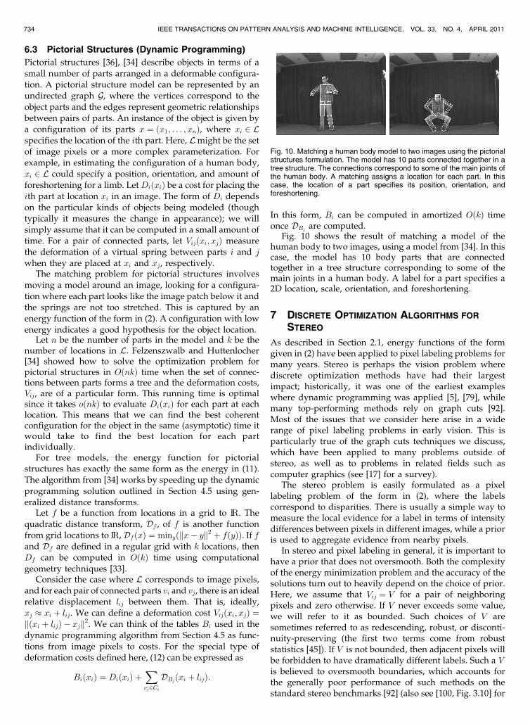
6.3 Pictorial Structures (Dynamic Programming)

Pictorial structures [36], [34] describe objects in terms of a

small number of parts arranged in a deformable configura-tion. A pictorial structure model can be represented by anundirected graph G, where the vertices correspond to the

object parts and the edges represent geometric relationshipsbetween pairs of parts. An instance of the object is given bya configuration of its parts x ¼ ðx1; . . . ; xnÞ, where xi 2 Lspecifies the location of the ith part. Here, Lmight be the setof image pixels or a more complex parameterization. Forexample, in estimating the configuration of a human body,

xi 2 L could specify a position, orientation, and amount offoreshortening for a limb. Let DiðxiÞ be a cost for placing theith part at location xi in an image. The form of Di depends

on the particular kinds of objects being modeled (thoughtypically it measures the change in appearance); we willsimply assume that it can be computed in a small amount oftime. For a pair of connected parts, let Vijðxi; xjÞ measure

the deformation of a virtual spring between parts i and j

when they are placed at xi and xj, respectively.The matching problem for pictorial structures involves

moving a model around an image, looking for a configura-tion where each part looks like the image patch below it andthe springs are not too stretched. This is captured by an

energy function of the form in (2). A configuration with lowenergy indicates a good hypothesis for the object location.

Let n be the number of parts in the model and k be thenumber of locations in L. Felzenszwalb and Huttenlocher[34] showed how to solve the optimization problem forpictorial structures in OðnkÞ time when the set of connec-tions between parts forms a tree and the deformation costs,Vij, are of a particular form. This running time is optimalsince it takes oðnkÞ to evaluate DiðxiÞ for each part at eachlocation. This means that we can find the best coherentconfiguration for the object in the same (asymptotic) time itwould take to find the best location for each partindividually.

For tree models, the energy function for pictorialstructures has exactly the same form as the energy in (11).The algorithm from [34] works by speeding up the dynamic

programming solution outlined in Section 4.5 using gen-eralized distance transforms.

Let f be a function from locations in a grid to IR. Thequadratic distance transform, Df , of f is another function

from grid locations to IR, DfðxÞ ¼ minyðkx� yk2 þ fðyÞÞ. If fand Df are defined in a regular grid with k locations, thenDf can be computed in OðkÞ time using computational

geometry techniques [33].Consider the case where L corresponds to image pixels,

and for each pair of connected parts vi and vj, there is an ideal

relative displacement lij between them. That is, ideally,xj xi þ lij. We can define a deformation cost Vijðxi; xjÞ ¼kðxi þ lijÞ � xjk2. We can think of the tables Bi used in the

dynamic programming algorithm from Section 4.5 as func-tions from image pixels to costs. For the special type ofdeformation costs defined here, (12) can be expressed as

BiðxiÞ ¼ DiðxiÞ þX

vj2CiDBjðxi þ lijÞ:

In this form, Bi can be computed in amortized OðkÞ timeonce DBj

are computed.Fig. 10 shows the result of matching a model of the

human body to two images, using a model from [34]. In thiscase, the model has 10 body parts that are connectedtogether in a tree structure corresponding to some of themain joints in a human body. A label for a part specifies a2D location, scale, orientation, and foreshortening.


STEREO

As described in Section 2.1, energy functions of the formgiven in (2) have been applied to pixel labeling problems formany years. Stereo is perhaps the vision problem wherediscrete optimization methods have had their largestimpact; historically, it was one of the earliest exampleswhere dynamic programming was applied [5], [79], whilemany top-performing methods rely on graph cuts [92].Most of the issues that we consider here arise in a widerange of pixel labeling problems in early vision. This isparticularly true of the graph cuts techniques we discuss,which have been applied to many problems outside ofstereo, as well as to problems in related fields such ascomputer graphics (see [17] for a survey).

The stereo problem is easily formulated as a pixellabeling problem of the form in (2), where the labelscorrespond to disparities. There is usually a simple way tomeasure the local evidence for a label in terms of intensitydifferences between pixels in different images, while a prioris used to aggregate evidence from nearby pixels.

In stereo and pixel labeling in general, it is important tohave a prior that does not oversmooth. Both the complexityof the energy minimization problem and the accuracy of thesolutions turn out to heavily depend on the choice of prior.Here, we assume that Vij ¼ V for a pair of neighboringpixels and zero otherwise. If V never exceeds some value,we will refer to it as bounded. Such choices of V aresometimes referred to as redescending, robust, or disconti-nuity-preserving (the first two terms come from robuststatistics [45]). If V is not bounded, then adjacent pixels willbe forbidden to have dramatically different labels. Such a Vis believed to oversmooth boundaries, which accounts forthe generally poor performance of such methods on thestandard stereo benchmarks [92] (also see [100, Fig. 3.10] for


Fig. 10. Matching a human body model to two images using the pictorialstructures formulation. The model has 10 parts connected together in atree structure. The connections correspond to some of the main joints ofthe human body. A matching assigns a location for each part. In thiscase, the location of a part specifies its position, orientation, andforeshortening.

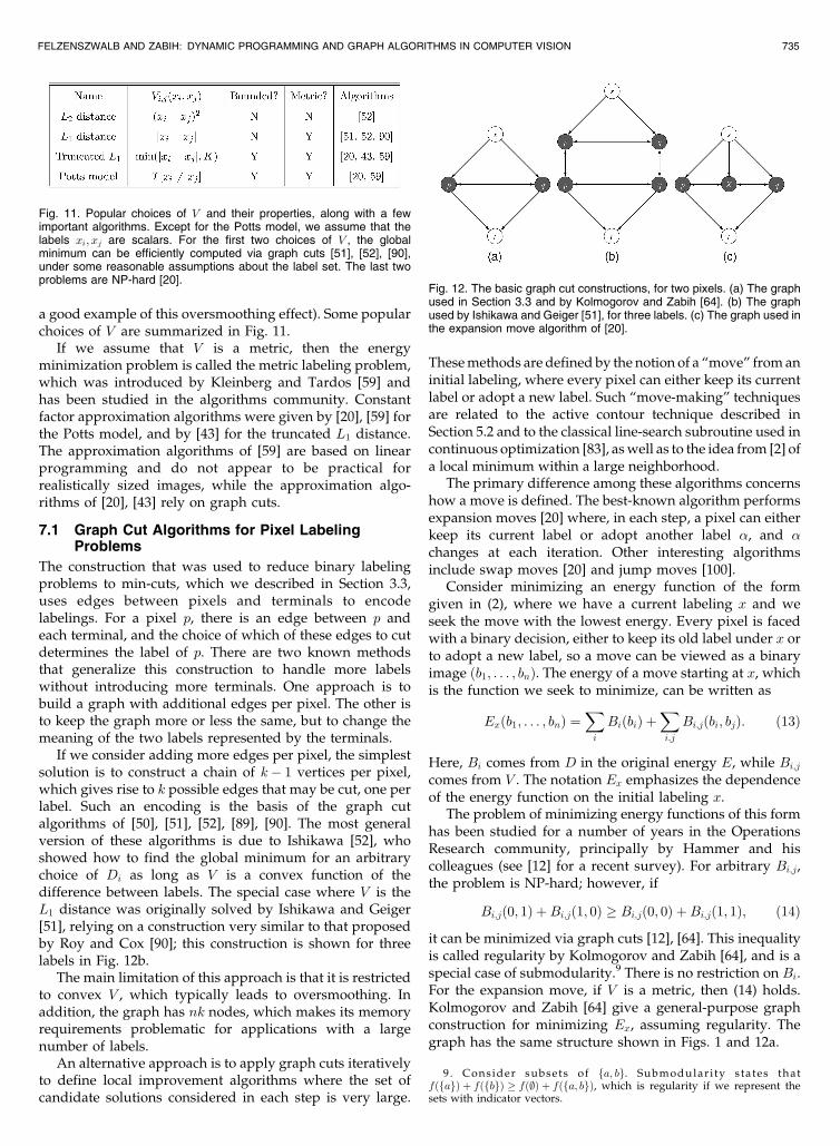
a good example of this oversmoothing effect). Some popularchoices of V are summarized in Fig. 11.

If we assume that V is a metric, then the energyminimization problem is called the metric labeling problem,which was introduced by Kleinberg and Tardos [59] andhas been studied in the algorithms community. Constantfactor approximation algorithms were given by [20], [59] forthe Potts model, and by [43] for the truncated L1 distance.The approximation algorithms of [59] are based on linearprogramming and do not appear to be practical forrealistically sized images, while the approximation algo-rithms of [20], [43] rely on graph cuts.

7.1 Graph Cut Algorithms for Pixel LabelingProblems

The construction that was used to reduce binary labelingproblems to min-cuts, which we described in Section 3.3,uses edges between pixels and terminals to encodelabelings. For a pixel p, there is an edge between p andeach terminal, and the choice of which of these edges to cutdetermines the label of p. There are two known methodsthat generalize this construction to handle more labelswithout introducing more terminals. One approach is tobuild a graph with additional edges per pixel. The other isto keep the graph more or less the same, but to change themeaning of the two labels represented by the terminals.

If we consider adding more edges per pixel, the simplestsolution is to construct a chain of k� 1 vertices per pixel,which gives rise to k possible edges that may be cut, one perlabel. Such an encoding is the basis of the graph cutalgorithms of [50], [51], [52], [89], [90]. The most generalversion of these algorithms is due to Ishikawa [52], whoshowed how to find the global minimum for an arbitrarychoice of Di as long as V is a convex function of thedifference between labels. The special case where V is theL1 distance was originally solved by Ishikawa and Geiger[51], relying on a construction very similar to that proposedby Roy and Cox [90]; this construction is shown for threelabels in Fig. 12b.

The main limitation of this approach is that it is restrictedto convex V , which typically leads to oversmoothing. Inaddition, the graph has nk nodes, which makes its memoryrequirements problematic for applications with a largenumber of labels.

An alternative approach is to apply graph cuts iterativelyto define local improvement algorithms where the set ofcandidate solutions considered in each step is very large.

These methods are defined by the notion of a “move” from aninitial labeling, where every pixel can either keep its currentlabel or adopt a new label. Such “move-making” techniquesare related to the active contour technique described inSection 5.2 and to the classical line-search subroutine used incontinuous optimization [83], as well as to the idea from [2] ofa local minimum within a large neighborhood.

The primary difference among these algorithms concernshow a move is defined. The best-known algorithm performsexpansion moves [20] where, in each step, a pixel can eitherkeep its current label or adopt another label �, and �changes at each iteration. Other interesting algorithmsinclude swap moves [20] and jump moves [100].

Consider minimizing an energy function of the formgiven in (2), where we have a current labeling x and weseek the move with the lowest energy. Every pixel is facedwith a binary decision, either to keep its old label under x orto adopt a new label, so a move can be viewed as a binaryimage ðb1; . . . ; bnÞ. The energy of a move starting at x, whichis the function we seek to minimize, can be written as

Exðb1; . . . ; bnÞ ¼X

i

BiðbiÞ þX

i;j

Bi;jðbi; bjÞ: ð13Þ

Here, Bi comes from D in the original energy E, while Bi;j

comes from V . The notation Ex emphasizes the dependenceof the energy function on the initial labeling x.

The problem of minimizing energy functions of this formhas been studied for a number of years in the OperationsResearch community, principally by Hammer and hiscolleagues (see [12] for a recent survey). For arbitrary Bi;j,the problem is NP-hard; however, if

Bi;jð0; 1Þ þBi;jð1; 0Þ � Bi;jð0; 0Þ þBi;jð1; 1Þ; ð14Þ

it can be minimized via graph cuts [12], [64]. This inequalityis called regularity by Kolmogorov and Zabih [64], and is aspecial case of submodularity.9 There is no restriction on Bi.For the expansion move, if V is a metric, then (14) holds.Kolmogorov and Zabih [64] give a general-purpose graphconstruction for minimizing Ex, assuming regularity. Thegraph has the same structure shown in Figs. 1 and 12a.


Fig. 11. Popular choices of V and their properties, along with a fewimportant algorithms. Except for the Potts model, we assume that thelabels xi; xj are scalars. For the first two choices of V , the globalminimum can be efficiently computed via graph cuts [51], [52], [90],under some reasonable assumptions about the label set. The last twoproblems are NP-hard [20].

Fig. 12. The basic graph cut constructions, for two pixels. (a) The graphused in Section 3.3 and by Kolmogorov and Zabih [64]. (b) The graphused by Ishikawa and Geiger [51], for three labels. (c) The graph used inthe expansion move algorithm of [20].

9. Consider subsets of fa; bg. Submodulari ty states thatfðfagÞ þ fðfbgÞ � fð;Þ þ fðfa; bgÞ, which is regularity if we represent thesets with indicator vectors.

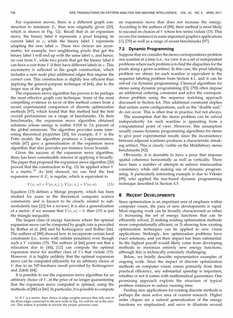
For expansion moves, there is a different graph con-struction to minimize Ex than was originally given [20],which is shown in Fig. 12c. Recall that in an expansionmove, the binary label 0 represents a pixel keeping itscurrent label in x, while the binary label 1 representsadapting the new label �. These two choices are asym-metric; for example, two neighboring pixels that get thebinary label 1 will end up with the same label �, and hence,no cost from V , while two pixels that get the binary label 0can have a cost from V if they have different labels in x. Thisasymmetry is reflected in the graph construction, whichincludes a new node plus additional edges that impose thecorrect cost. This construction is slightly less efficient thanapplying the general-purpose technique of [64], due to thelarger size of the graph.

The expansion move algorithm has proven to be perhapsthe most effective graph cuts technique. Some of the mostcompelling evidence in favor of this method comes from arecent experimental comparison of discrete optimizationmethods [97], which found that this method had the bestoverall performance on a range of benchmarks. On theirbenchmarks, the expansion move algorithm obtainedsolutions whose energy is within 0.018 to 3.6 percent ofthe global minimum. The algorithm provides some inter-esting theoretical properties [20]; for example, if V is thePotts model, the algorithm produces a 2-approximation,while [67] gave a generalization of the expansion movealgorithm that also provides per-instance lower bounds.

Given the success of the expansion move algorithm,there has been considerable interest in applying it broadly.The paper that proposed the expansion move algorithm [20]proved that the construction in Fig. 12c be applied when Vis a metric.10 As [64] showed, we can find the bestexpansion move if Ex is regular, which is equivalent to

V ðxi; �Þ þ V ð�; xjÞ � V ðxi; xjÞ þ V ð�; �Þ: ð15Þ

Equation (15) defines a Monge property, which has beenstudied for years in the theoretical computer sciencecommunity and is known to be closely related to sub-modularity (see [22] for a review). It is also a generalizationof a metric; if we assume that V ð�; �Þ ¼ 0, then (15) is justthe triangle inequality.

The largest class of energy functions where the optimalexpansion move can be computed by graph cuts is providedby Rother et al. [88] and by Kolmogorov and Rother [66].The authors of [88] showed how to incorporate certain hardconstraints (i.e., terms with infinite penalties) even thoughsuch a V violates (15). The authors of [66] point out that arelaxation due to [44], [12] can compute the optimalexpansion move for another class of V s that violate (15).However, it is highly unlikely that the optimal expansionmove can be computed efficiently for an arbitrary choice ofV due to an NP-hardness result provided by Kolmogorovand Zabih [64].

It is possible to use the expansion move algorithm for anarbitrary choice of V , at the price of no longer guaranteeingthat the expansion move computed is optimal, using themethods of [88] or [66]. In particular, it is possible to compute

an expansion move that does not increase the energy.According to the authors of [88], their method is most likelyto succeed on choices of V where few terms violate (15). Thisoccurs (for instance) in some important graphics applications[1], [70] as well as a range of recent benchmarks [97].

7.2 Dynamic Programming

Suppose that we consider the stereo correspondence problemone scanline at a time (i.e., we view it as a set of independentproblems where each problem is to find the disparities for thepixels along a given scanline). In this case, the pixel labelingproblem we obtain for each scanline is equivalent to thesequence labeling problem from Section 4.1, and it can besolved via dynamic programming. Classical algorithms forstereo using dynamic programming ([5], [79]) often imposean additional ordering constraint and solve the correspon-dence problem using the sequence matching approachdiscussed in Section 4.6. This additional constraint impliesthat certain scene configurations, such as the “double nail,”do not occur. This is often true in practice, but not always.

The assumption that the stereo problem can be solvedindependently for each scanline is appealing from acomputational point of view. However, this assumptionusually causes dynamic programming algorithms for stereoto give poor experimental results since the inconsistencybetween adjacent scanlines produces a characteristic streak-ing artifact. This is clearly visible on the Middlebury stereobenchmarks [92].

Obviously, it is desirable to have a prior that imposesspatial coherence horizontally as well as vertically. Therehave been a number of attempts to enforce interscanlineconsistency while still making use of dynamic program-ming. A particularly interesting example is due to Veksler[99], who applied the tree-based dynamic programmingtechnique described in Section 4.5.

8 RECENT DEVELOPMENTS

Since optimization is an important area of emphasis withincomputer vision, the pace of new developments is rapid.Most ongoing work can be broadly characterized as either1) increasing the set of energy functions that can beefficiently solved, 2) making existing optimization methodsmore computationally efficient, or 3) showing how existingoptimization techniques can be applied to new visionapplications. Strikingly, few optimization problems haveexact solutions, and yet their impact has been substantial.So the highest payoff would likely come from developingmethods to minimize entirely new energy functions,although this is technically extremely challenging.

Below, we briefly describe representative examples ofongoing work. Since the impact of discrete optimizationmethods on computer vision comes primarily from theirpractical efficiency, any substantial speedup is important,whether or not it comes with mathematical guarantees. Onepromising approach exploits the structure of typicalproblem instances to reduce running time.

Finding new applications for existing discrete methods isperhaps the most active area of current research. Higherorder cliques are a natural generalization of the energyfunctions we emphasized, and serve to illustrate several


10. If V is a metric, their choice of edge weights ensures that only one ofthe three edges connected to the new node in Fig. 12c will be cut in the min-cut. This makes it possible to encode the proper pairwise costs.

important techniques. The techniques we describe below,which draw on relaxation methods, do not solve the discreteoptimization problem exactly, and there is currently no proofthat the solution computed is close to the global minimum.

8.1 Data-Dependent Speedups

Some existing methods can be made substantially faster inpractice by taking advantage of usual properties of theinput data. For example, in dynamic programming, it is notalways necessary to fill in the entire set of tables Bi

described in Section 4. For some problems, if we useDijkstra’s algorithm, A* search, or generalizations of thesemethods [35], many of the entries in these tables will remainempty when the optimal solution is found. Similarly,coarse-to-fine methods can often exploit regularities in theinput data to good effect [86], [85].

A common property of these techniques is that they donot usually improve the worst-case running time of theenergy minimization problem. Instead, they may useheuristics that significantly speed up the computation ontypical instances. For example, [40] considers the problem ofroad detection and gives an algorithm inspired in the“Twenty Questions” game for finding the most likelylocation of the road while doing as little computation aspossible.

In some cases, it is possible to prove good expectedrunning time if we assume a particular distribution on theinput. The method for road detection in [26] assumes thatthe input comes from a particular distribution to obtain analgorithm that will quickly find an optimal or near-optimalsolution with high probability. This basic idea firstappeared in [55] for the problem of finding an optimalpath from the root to a leaf in a binary tree with randomcosts. If the costs on each edge are assumed to beindependent, [55] shows how a path of near-optimal costcan be found very quickly with high probability.

The method in [85] is particularly interesting in the waythat it combines dynamic programming with coarse-to-finecomputation to obtain an algorithm that is still polynomialin the worst case. Consider the sequence labeling problemfrom Section 4.1. Dynamic programming can find anoptimal labeling in Oðnk2Þ time, where n is the number ofelements in the sequence and k is the number of possiblelabels. Even though the running time is polynomial in thenumber of labels, if this is very large, the computation willbe infeasible. The method in [85] constructs a series ofcoarse approximations to the original problem by aggre-gating possible labels for each element into “superlabels.”Initially, we have a small number of possible superlabelsfor each element. An optimal solution to the coarseproblem is found using standard dynamic programmingand the superlabel that is assigned to an element isrefined into a set of smaller superlabels to define a newproblem. The process is iterated until the optimal solutionuses only singleton labels. If the coarse problems aredefined in a particular way, the final solution is a globalminimum of the original problem. In many cases, thisleads to a much faster algorithm in practice. It is possibleto prove that the method has good expected running timeif we assume that the input data have certain regularities,but in the worst case, the method can actually be slower

than the dynamic programming solution to the originalproblem.

8.2 Efficient Algorithms for Higher Order Cliques

Many of the energy functions we have discussed are of theform given in (2), where the prior involves pairs of adjacentpixels. Yet, many natural priors cannot be expressed thisway; for example, to limit the curvature of a boundaryrequires considering three or more adjacent pixels at a time.It is straightforward to incorporate such a constraint in adynamic programming algorithm for sequence labeling, asdescribed in Section 4.3, at some additional computationalcost. It is much more difficult to incorporate suchconstraints into the energy functions that arise in pixellabeling problems such as stereo.

Dynamic programming cannot be easily applied to pixellabeling problems because the grid has high treewidth.Priors that depend directly on more than two variables arereferred to as “higher order cliques” (the term comes fromthe MRF literature). Certain higher order cliques can behandled by generalizing the graph cut methods of [20]; forexample, [62] showed how to do this for a naturalgeneralization of the Potts model where a group ofvariables pays a uniform penalty unless they all take onthe same value.

A representative example of current research is providedby [49], which draws on several important developments ingraph cuts. To use a move-making technique such as theexpansion move algorithm with higher order cliques, it isnecessary to solve a binary problem that is more complexthan (13). The main result of [49] is a transformation of thismore complex binary problem into the form of (13), at theprice of introducing additional binary variables.

There are two additional challenges that [49] addresses.First, the resulting binary problem is usually not regular, somax-flow cannot be used to solve it exactly. Ishikawa [49]relies on a relaxation technique originally invented by Borosand Hammer [12], which was introduced into computervision by Kolmogorov and Rother [66]. This technique(called either roof duality or QPBO) uses max-flow tocompute a partially optimal solution to the binary problem.Only a subset of the variables is given a value, but if westart at an arbitrary labeling and assign this subset theircorresponding values, the energy will not increase. Thisimplies that there is an optimal solution that is an extensionof these values. While this relaxation method can performwell in practice, there are few theoretical guarantees (forexample, it is possible that no variable is given a value).

The second challenge that [49] addresses is that for someapplications, a better move-making algorithm is neededthan expansion moves or swap moves. A generalizationknown as fusion moves [71] can be applied to many suchproblems. In a fusion move, two candidate solutions aremerged and every pixel makes a binary decision as to whichcandidate solution’s label to adopt. The expansion movealgorithm can be viewed as a fusion move, where onecandidate solution is the current labeling and the otherassigns a single label to every pixel.

By relying on roof duality and fusion moves, the mainresult of [49] can be applied to several applications withhigher order cliques. While these methods use established


graph cut techniques as subroutines, they do not guarantee

an exact solution. Yet, they can perform quite well for

practical applications such as [103].

9 CONCLUSIONS

The power of discrete optimization techniques such asdynamic programming and graph algorithms arises fromexploiting the specific structure of important problems.These algorithms often provide strong guarantees about thequality of the solutions they find, which allows for a cleanseparation between how a problem is formulated (thechoice of objective function) and how the problem is solved(the choice of optimization algorithm). The methods areversatile and arise in very different vision applications; forexample, sequence matching via dynamic programmingcan be used for both shape recognition and stereo.Similarly, min-cut algorithms can be used both for stereoand binary image segmentation. These apparently unre-lated problems share structure that can be exploited bydiscrete optimization methods.

ACKNOWLEDGMENTS

The authors received help from many people with the

content and presentation of this material, and especially wish

to thank Jon Kleinberg, David Kriegman, Eva Tardos, and

Phil Torr, as well as the anonymous reviewers. This research

has been supported by the US National Science Foundation

(NSF) under grants IIS-0746569 and IIS-0803705 and by the

US National Institutes of Health (NIH) under grants

R21EB008138 and P41RR023953.

REFERENCES

[1] A. Agarwala, M. Dontcheva, M. Agrawala, S. Drucker, A.Colburn, B. Curless, D. Salesin, and M. Cohen, “Interactive DigitalPhotomontage,” ACM Trans. Graphics, vol. 23, no. 3, pp. 292-300,2004.

[2] R.K. Ahuja, O. Ergun, J.B. Orlin, and A.P. Punnen, “A Survey ofVery Large-Scale Neighborhood Search Techniques,” DiscreteApplied Math., vol. 123, nos. 1-3, pp. 75-102, 2002.

[3] A. Amini, T. Weymouth, and R. Jain, “Using Dynamic Program-ming for Solving Variational Problems in Vision,” IEEE Trans.Pattern Analysis and Machine Intelligence, vol. 12, no. 9, pp. 855-867,Sept. 1990.

[4] Y. Amit and A. Kong, “Graphical Templates for Model Registra-tion,” IEEE Trans. Pattern Analysis and Machine Intelligence, vol. 18,no. 3, pp. 225-236, Mar. 1996.

[5] H.H. Baker and T.O. Binford, “Depth from Edge and IntensityBased Stereo,” Proc. Int’l Joint Conf. Artificial Intelligence, pp. 631-636, 1981.

[6] S. Barnard, “Stochastic Stereo Matching over Scale,” Int’l J.Computer Vision, vol. 3, no. 1, pp. 17-32, 1989.

[7] R. Basri, L. Costa, D. Geiger, and D. Jacobs, “Determining theSimilarity of Deformable Shapes,” Vision Research, vol. 38,pp. 2365-2385, 1998.

[8] R. Bellman, Dynamic Programming. Princeton Univ. Press, 1957.[9] S. Belongie, J. Malik, and J. Puzicha, “Shape Matching and

Object Recognition Using Shape Contexts,” IEEE Trans. PatternAnalysis and Machine Intelligence, vol. 24, no. 4, pp. 509-522, Apr.2002.

[10] S. Birchfield and C. Tomasi, “Multiway Cut for Stereo and Motionwith Slanted Surfaces,” Proc. IEEE Int’l Conf. Computer Vision,pp. 489-495, 1999.

[11] A. Blake and A. Zisserman, Visual Reconstruction. MIT Press, 1987.[12] E. Boros and P.L. Hammer, “Pseudo-Boolean Optimization,”

Discrete Applied Math., vol. 123, nos. 1-3, 2002.

[13] S. Boyd and L. Vandenberghe, Convex Optimization. CambridgeUniv. Press, 2004.

[14] Y. Boykov and G. Funka-Lea, “Graph Cuts and Efficient N-DImage Segmentation,” Int’l J. Computer Vision, vol. 70, pp. 109-131,2006.

[15] Y. Boykov and M.-P. Jolly, “Interactive Graph Cuts for OptimalBoundary and Region Segmentation of Objects in N-D Images,”Proc. IEEE Int’l Conf. Computer Vision, pp. I:105-I:112, 2001.

[16] Y. Boykov and V. Kolmogorov, “An Experimental Comparison ofMin-Cut/Max-Flow Algorithms for Energy Minimization inVision,” IEEE Trans. Pattern Analysis and Machine Intelligence,vol. 26, no. 9, pp. 1124-1137, Sept. 2004.

[17] Y. Boykov and O. Veksler, “Graph Cuts in Vision and Graphics:Theories and Applications,” Math. Models in Computer Vision: TheHandbook, N. Paragios, ed., pp. 79-95, Springer, 2005.

[18] Y. Boykov, O. Veksler, and R. Zabih, “Markov Random Fieldswith Efficient Approximations,” Proc. IEEE Conf. Computer Visionand Pattern Recognition, pp. 648-655, 1998.

[19] Y. Boykov, O. Veksler, and R. Zabih, “Fast Approximate EnergyMinimization via Graph Cuts,” Proc. IEEE Int’l Conf. ComputerVision, pp. 377-384, 1999.

[20] Y. Boykov, O. Veksler, and R. Zabih, “Fast Approximate EnergyMinimization via Graph Cuts,” IEEE Trans. Pattern Analysis andMachine Intelligence, vol. 23, no. 11, pp. 1222-1239, Nov. 2001.

[21] M.Z. Brown, D. Burschka, and G.D. Hager, “Advances inComputational Stereo,” IEEE Trans. Pattern Analysis and MachineIntelligence, vol. 25, no. 8, pp. 993-1008, Aug. 2003.

[22] R. Burkard, B. Klinz, and R. Rudolf, “Perspectives of MongeProperties in Optimization,” Discrete and Applied Math., vol. 70,no. 2, pp. 95-161, 1996.

[23] W. Cook, W. Cunningham, W. Pulleyblank, and A. Schrijver,Combinatorial Optimization. John Wiley & Sons, 1998.

[24] T.H. Cormen, C.E. Leiserson, and R.L. Rivest, Introduction toAlgorithms. MIT Press and McGraw-Hill, 1989.

[25] J. Coughlan, A. Yuille, C. English, and D. Snow, “EfficientDeformable Template Detection and Localization without UserInitialization,” Computer Vision and Image Understanding, vol. 78,no. 3, pp. 303-319, June 2000.

[26] J. Coughlan and A.L. Yuille, “Bayesian A* Tree Search withExpected O(N) Node Expansions: Applications to Road Track-ing,” Neural Computation, vol. 14, no. 8, pp. 1929-1958, 2006.

[27] W.H. Cunningham, “Minimum Cuts, Modular Functions, andMatroid Polyhedra,” Networks, vol. 15, pp. 205-215, 1985.

[28] E. Dahlhaus, D. Johnson, C. Papadimitriou, P. Seymour, and M.Yannakakis, “The Complexity of Multiterminal Cuts,” SIAM J.Computing, vol. 23, no. 4, pp. 864-894, 1994.

[29] T.J. Darrell, D. Demirdjian, N. Checka, and P.F. Felzenszwalb,“Plan-View Trajectory Estimation with Dense Stereo BackgroundModels,” Proc. IEEE Int’l Conf. Computer Vision, 2001.

[30] F. Dellaert, “Monte Carlo EM for Data-Association and ItsApplications in Computer Vision,” PhD thesis, Carnegie MellonUniv., Sept. 2001.

[31] E.W. Dijkstra, “A Note on Two Problems in Connection withGraphs,” Numerical Math., vol. 1, pp. 269-271, 1959.

[32] P.F. Felzenszwalb, “Representation and Detection of DeformableShapes,” IEEE Trans. Pattern Analysis and Machine Intelligence,vol. 27, no. 2, pp. 208-220, Feb. 2005.

[33] P.F. Felzenszwalb and D.P. Huttenlocher, “Distance Transforms ofSampled Functions,” Technical Report TR2004-1963, Faculty ofComputing and Information Science, Cornell Univ., Sept. 2004.

[34] P.F. Felzenszwalb and D.P. Huttenlocher, “Pictorial Structures forObject Recognition,” Int’l J. Computer Vision, vol. 61, no. 1, pp. 55-79, 2005.

[35] P.F. Felzenszwalb and D. McAllester, “The Generalized A*Architecture,” J. Artificial Intelligence Research, vol. 29, pp. 153-190, 2007.

[36] M.A. Fischler and R.A. Elschlager, “The Representation andMatching of Pictorial Structures,” IEEE Trans. Computers, vol. 22,no. 1, pp. 67-92, Jan. 1973.

[37] L. Ford and D. Fulkerson, Flows in Networks. Princeton Univ.Press, 1962.

[38] M. Garey and D. Johnson, Computers and Intractability.W.H. Freeman and Co., 1979.

[39] D. Geiger, A. Gupta, L.A. Costa, and J. Vlontzos, “Dynamic-Programming for Detecting, Tracking, and Matching DeformableContours,” IEEE Trans. Pattern Analysis and Machine Intelligence,vol. 17, no. 3, pp. 294-302, Mar. 1995.


[40] D. Geman and B. Jedynak, “An Active Testing Model for TrackingRoads in Satellite Images,” IEEE Trans. Pattern Analysis andMachine Intelligence, vol. 18, no. 1, pp. 1-14, Jan. 1996.

[41] S. Geman and D. Geman, “Stochastic Relaxation, Gibbs Distribu-tions, and the Bayesian Restoration of Images,” IEEE Trans. PatternAnalysis and Machine Intelligence, vol. 6, no. 6, pp. 721-741, Nov.1984.

[42] D. Greig, B. Porteous, and A. Seheult, “Exact Maximum aPosteriori Estimation for Binary Images,” J. Royal Statistical Soc.,Series B, vol. 51, no. 2, pp. 271-279, 1989.

[43] A. Gupta and E. Tardos, “A Constant Factor ApproximationAlgorithm for a Class of Classification Problems,” Proc. ACMSymp. Theoretical Computer Science, 2000.

[44] P.L. Hammer, P. Hansen, and B. Simeone, “Roof Duality,Complementation and Persistency in Quadratic 0-1 Optimiza-tion,” Math. Programming, vol. 28, pp. 121-155, 1984.

[45] F.R. Hampel, E.M. Ronchetti, P.J. Rousseeuw, and W.A. Stahel,Robust Statistics: The Approach Based on Influence Functions. Wiley,1986.

[46] M.J. Hanna, “Computer Matching of Areas in Stereo Images,”PhD thesis, Stanford Univ., 1974.

[47] J. Holland, Adaptation in Natural and Artificial Systems: AnIntroductory Analysis with Applications to Biology, Control, andArtificial Intelligence. Univ. of Michigan Press, 1975.

[48] B.K.P. Horn and B. Schunk, “Determining Optical Flow,” ArtificialIntelligence, vol. 17, pp. 185-203, 1981.

[49] H. Ishikawa, “Higher-Order Clique Reduction in Binary GraphCut,” Proc. IEEE Conf. Computer Vision and Pattern Recognition,2009.

[50] H. Ishikawa and D. Geiger, “Occlusions, Discontinuities, andEpipolar Lines in Stereo,” Proc. European Conf. Computer Vision,pp. 232-248, 1998.

[51] H. Ishikawa and D. Geiger, “Segmentation by Grouping Junc-tions,” Proc. IEEE Conf. Computer Vision and Pattern Recognition,pp. 125-131, 1998.

[52] H. Ishikawa, “Exact Optimization for Markov Random Fields withConvex Priors,” IEEE Trans. Pattern Analysis and MachineIntelligence, vol. 25, no. 10, pp. 1333-1336, Oct. 2003.

[53] I.H. Jermyn and H. Ishikawa, “Globally Optimal Regions andBoundaries as Minimum Ratio Weight Cycles,” IEEE Trans.Pattern Analysis and Machine Intelligence, vol. 23, no. 10, pp. 1075-1088, Oct. 2001.

[54] R. Kannan, S. Vempala, and A. Vetta, “On Clusterings: Good, Bad,and Spectral,” J. ACM, vol. 51, no. 3, pp. 497-515, 2004.

[55] R.M. Karp and J. Pearl, “Searching for an Optimal Path in a Treewith Random Costs,” Artificial Intelligence, vol. 21, no. 1, pp. 99-116, 1983.

[56] M. Kass, A. Witkin, and D. Terzopoulos, “Snakes: Active ContourModels,” Int’l J. Computer Vision, vol. 1, no. 4, pp. 321-331, 1987.

[57] J. Kim, V. Kolmogorov, and R. Zabih, “Visual CorrespondenceUsing Energy Minimization and Mutual Information,” Proc. IEEEInt’l Conf. Computer Vision, pp. 1033-1040, 2003.

[58] J. Kim and R. Zabih, “Automatic Segmentation of Contrast-Enhanced Image Sequences,” Proc. IEEE Int’l Conf. ComputerVision, pp. 502-509, 2003.

[59] J. Kleinberg and E. Tardos, “Approximation Algorithms forClassification Problems with Pairwise Relationships: MetricLabeling and Markov Random Fields,” J. ACM, vol. 49, no. 5,pp. 616-639, 2002.

[60] J. Kleinberg and E. Tardos, Algorithm Design. Addison Wesley,2005.

[61] D. Knuth, “A Generalization of Dijkstra’s Algorithm,” InformationProcessing Letters, vol. 6, no. 1, pp. 1-5, Feb. 1977.

[62] P. Kohli, M.P. Kumar, and P.H.S. Torr, “P3 and Beyond: MoveMaking Algorithms for Solving Higher Order Functions,” IEEETrans. Pattern Analysis and Machine Intelligence, vol. 31, no. 9,pp. 1645-1656, Sept. 2009.

[63] P. Kohli and P. Torr, “Efficiently Solving Dynamic MarkovRandom Fields Using Graph Cuts,” Proc. IEEE Int’l Conf. ComputerVision, 2005.

[64] V. Kolmogorov and R. Zabih, “What Energy Functions Can BeMinimized via Graph Cuts?” IEEE Trans. Pattern Analysis andMachine Intelligence, vol. 26, no. 2, pp. 147-159, Feb. 2004.

[65] V. Kolmogorov, A. Criminisi, A. Blake, G. Cross, and C. Rother,“Probabilistic Fusion of Stereo with Color and Contrast for Bi-Layer Segmentation,” IEEE Trans. Pattern Analysis and MachineIntelligence, vol. 28, no. 9, pp. 1480-1492, Sept. 2006.

[66] V. Kolmogorov and C. Rother, “Minimizing NonsubmodularFunctions with Graph Cuts—A Review,” IEEE Trans. PatternAnalysis and Machine Intelligence, vol. 29, no. 7, pp. 1274-1279, July2007.

[67] N. Komodakis and G. Tziritas, “A New Framework for Approx-imate Labeling via Graph Cuts,” Proc. IEEE Int’l Conf. ComputerVision, 2005.

[68] B. Korte and J. Vygen, Combinatorial Optimization: Theory andAlgorithms. Springer, 2005.

[69] A. Krause, A. Singh, and C. Guestrin, “Near-Optimal SensorPlacements in Gaussian Processes: Theory, Efficient Algorithmsand Empirical Studies,” J. Machine Learning Research, vol. 9,pp. 235-284, 2008.

[70] V. Kwatra, A. Schodl, I. Essa, G. Turk, and A. Bobick, “GraphcutTextures: Image and Video Synthesis Using Graph Cuts,” ACMTrans. Graphics, vol. 22, pp. 277-286, 2003.

[71] V. Lempitsky, C. Rother, S. Roth, and A. Blake, “Fusion Moves forMarkov Random Field Optimization,” IEEE Trans. Pattern Analysisand Machine Intelligence, vol. 32, no. 8, pp. 1392-1405, Aug. 2010.

[72] M.H. Lin and C. Tomasi, “Surfaces with Occlusions from LayeredStereo,” IEEE Trans. Pattern Analysis and Machine Intelligence,vol. 26, no. 8, pp. 1073-1078, Aug. 2004.

[73] H. Ling and D.W. Jacobs, “Using the Inner-Distance forClassification of Articulated Shapes,” Proc. IEEE Conf. ComputerVision and Pattern Recognition, pp. II:719-II:726, 2005.

[74] M. Maes, “On a Cyclic String-to-String Correction Problem,”Information Processing Letters, vol. 35, no. 2, pp. 73-78, June 1990.

[75] D.R. Martin, C.C. Fowlkes, and J. Malik, “Learning to DetectNatural Image Boundaries Using Local Brightness, Color, andTexture Cues,” IEEE Trans. Pattern Analysis and Machine Intelli-gence, vol. 26, no. 5, pp. 530-549, May 2004.

[76] N. Metropolis, A.W. Rosenbluth, M.N. Rosenbluth, A.H. Teller,and E. Teller, “Equations of State Calculations by Fast ComputingMachines,” J. Chemical Physics, vol. 21, pp. 1087-1091, 1953.

[77] U. Montanari, “On the Optimal Detection of Curves in NoisyPictures,” Comm. ACM, vol. 14, no. 5, pp. 335-345, 1971.

[78] E.N. Mortensen and W.A. Barrett, “Intelligent Scissors for ImageComposition,” Proc. ACM SIGGRAPH, pp. 191-198, 1995.

[79] Y. Ohta and T. Kanade, “Stereo by Intra- and Inter-Scanline SearchUsing Dynamic Programming,” IEEE Trans. Pattern Analysis andMachine Intelligence, vol. 7, no. 2, pp. 139-154, Mar. 1985.

[80] C. Papadimitriou and K. Stieglitz, Combinatorial Optimization:Algorithms and Complexity. Prentice Hall, 1982.

[81] V.I. Pavlovic, R. Sharma, and T.S. Huang, “Visual Interpretation ofHand Gestures for Human-Computer Interaction: A Review,”IEEE Trans. Pattern Analysis and Machine Intelligence, vol. 19, no. 7,pp. 677-695, July 1997.

[82] T. Poggio, V. Torre, and C. Koch, “Computational Vision andRegularization Theory,” Nature, vol. 317, pp. 314-319, 1985.

[83] W. Press, S. Teukolsky, W. Vetterling, and B. Flannery, NumericalRecipes in C. Cambridge Univ. Press, 1992.

[84] L. Rabiner, “A Tutorial on Hidden Markov Models and SelectedApplications in Speech Recognition,” Proc. IEEE, vol. 77, no. 2,pp. 257-286, Feb. 1989.

[85] C. Raphael, “Coarse-to-Fine Dynamic Programming,” IEEE Trans.Pattern Analysis and Machine Intelligence, vol. 23, no. 12, pp. 1379-1390, Dec. 2001.

[86] C. Raphael and S. Geman, “A Grammatical Approach to MineDetection,” Proc. Conf. SPIE, pp. 316-337, 1997.

[87] C. Rother, V. Kolmogorov, and A. Blake, ““GrabCut”—InteractiveForeground Extraction Using Iterated Graph Cuts,” ACM Trans.Graphics, vol. 23, no. 3, pp. 309-314, 2004.

[88] C. Rother, S. Kumar, V. Kolmogorov, and A. Blake, “DigitalTapestry,” Proc. IEEE Conf. Computer Vision and Pattern Recogni-tion, 2005.

[89] S. Roy, “Stereo without Epipolar Lines: A Maximum FlowFormulation,” Int’l J. Computer Vision, vol. 1, no. 2, pp. 1-15, 1999.

[90] S. Roy and I. Cox, “A Maximum-Flow Formulation of the N-Camera Stereo Correspondence Problem,” Proc. IEEE Int’l Conf.Computer Vision, 1998.

[91] I. Satoru, F. Lisa, and F. Satoru, “A Combinatorial, StronglyPolynomial Algorithm for Minimizing Submodular Functions,”J. ACM, vol. 48, no. 4, pp. 761-777, 2001.

[92] D. Scharstein and R. Szeliski, “A Taxonomy and Evaluation ofDense Two-Frame Stereo Correspondence Algorithms,” Int’l J.Computer Vision, vol. 47, pp. 7-42, 2002.


[93] T. Schoenemann and D. Cremers, “Matching Non-RigidlyDeformable Shapes across Images: A Globally Optimal Solution,”Proc. IEEE Conf. Computer Vision and Pattern Recognition, pp. 1-6,2008.

[94] T.B. Sebastian, P.N. Klein, and B.B. Kimia, “On Aligning Curves,”IEEE Trans. Pattern Analysis and Machine Intelligence, vol. 25, no. 1,pp. 116-124, Jan. 2003.

[95] A. Shashua and S. Ullman, “Structural Saliency: The Detection ofGlobally Salient Structures Using a Locally Connected Network,”Proc. IEEE Int’l Conf. Computer Vision, pp. 321-327, 1988.

[96] J. Shi and J. Malik, “Normalized Cuts and Image Segmentation,”IEEE Trans. Pattern Analysis and Machine Intelligence, vol. 22, no. 8,pp. 888-905, Aug. 2000.

[97] R. Szeliski, R. Zabih, D. Scharstein, O. Veksler, V. Kolmogorov, A.Agarwala, M. Tappen, and C. Rother, “A Comparative Study ofEnergy Minimization Methods for Markov Random Fields,” IEEETrans. Pattern Analysis and Machine Intelligence, vol. 30, no. 6,pp. 1068-1080, June 2008.

[98] A. Tikhonov and V. Arsenin, Solutions of Ill-Posed Problems.Winston and Sons, 1977.

[99] O. Veksler, “Stereo Correspondence by Dynamic Programming ona Tree,” Proc. IEEE Conf. Computer Vision and Pattern Recognition,pp. 384-390, 2005.

[100] O. Veksler, “Efficient Graph-Based Energy Minimization Methodsin Computer Vision,” PhD thesis, Cornell Univ., 1999.

[101] M. Wainwright, T. Jaakkola, and A. Willsky, “Map Estimation viaAgreement on Trees: Message-Passing and Linear Programming,”IEEE Trans. Information Theory, vol. 5, no. 11, pp. 3697-3717, Nov.2005.

[102] Y. Weiss, C. Yanover, and T. Meltzer, “Map Estimation, LinearProgramming and Belief Propagation with Convex Free Ener-gies,” Proc. Conf. Uncertainty in Artificial Intelligence, 2007.

[103] O. Woodford, P. Torr, I. Reid, and A. Fitzgibbon, “Global StereoReconstruction Under Second-Order Smoothness Priors,” IEEETrans. Pattern Analysis and Machine Intelligence, vol. 31, no. 12,pp. 2115-2128, Dec. 2009.

Pedro F. Felzenszwalb received the BS degreefrom Cornell University in 1999 and the MS andPhD degrees from the Massachusetts Instituteof Technology (MIT) in 2001 and 2003, respec-tively, all in computer science. After leaving MIT,he spent one year as a postdoctoral researcherat Cornell University. He joined the Departmentof Computer Science at the University ofChicago in 2004, where he is currently anassociate professor. His work has been sup-

ported by the US National Science Foundation (NSF), including aCAREER Award received in 2008. His main research interests includecomputer vision, geometric algorithms, and artificial intelligence. He willbe a program chair for the 2011 IEEE Conference on Computer Visionand Pattern Recognition (CVPR) and is currently an associate editor ofthe IEEE Transactions on Pattern Analysis and Machine Intelligence. Heis a member of the IEEE Computer Society.

Ramin Zabih received the BS and MS degreesfrom the Massachusetts Institute of Technologyand the PhD degree from Stanford University.He is a professor of computer science at CornellUniversity, where he has taught since 1994.Beginning in 2001, he has also held a jointappointment at Cornell’s Weill Medical Collegein the Department of Radiology. His researchinterests lie in discrete optimization in earlyvision and its applications in areas such as

stereo and medicine. He is best known for his group’s work on graphcuts for which he shared the Best Paper Prize at ECCV in 2002. Heserved as a program chair for CVPR in 2007 and will be a general chairfor CVPR in 2013. He was appointed to the editorial board of the IEEETransactions on Pattern Analysis and Machine Intelligence in 2005, andsince 2009, has served as the editor-in-chief. He is a senior member ofthe IEEE and a member of the IEEE Computer Society.

. For more information on this or any other computing topic,please visit our Digital Library at www.computer.org/publications/dlib.


Documents

IEEE TRANSACTIONS ON PATTERN ANALYSIS AND … · problem is solved (the optimization ... APRIL 2011 721. P.F. Felzenszwalb is with the Department ... 0162-8828/11/$26.00 2011 IEEE