IEEE TRANSACTIONS ON IMAGE PROCESSING, VOL. … · Iterative Truncated Arithmetic Mean Filter and Its Properties Xudong Jiang, Senior Member, IEEE ... metic operations, which owns

IEEE TRANSACTIONS ON IMAGE PROCESSING, VOL. 21, NO. 4, APRIL 2012 1537

Iterative Truncated Arithmetic Mean Filter andIts Properties

Xudong Jiang, Senior Member, IEEE

Abstract—The arithmetic mean and the order statistical medianare two fundamental operations in signal and image processing.They have their own merits and limitations in noise attenuationand image structure preservation. This paper proposes an itera-tive algorithm that truncates the extreme values of samples in thefilter window to a dynamic threshold. The resulting nonlinear filtershows some merits of both the fundamental operations. Some dy-namic truncation thresholds are proposed that guarantee the filteroutput, starting from the mean, to approach the median of theinput samples. As a by-product, this paper unveils some statisticsof a finite data set as the upper bounds of the deviation of the me-dian from the mean. Some stopping criteria are suggested to facili-tate edge preservation and noise attenuation for both the long- andshort-tailed distributions. Although the proposed iterative trun-cated mean (ITM) algorithm is not aimed at the median, it offers away to estimate the median by simple arithmetic computing. Someproperties of the ITM filters are analyzed and experimentally ver-ified on synthetic data and real images.

Index Terms—Edge preservation, image noise attenuation, me-dian approximation, median filter, nonlinear filter.

I. INTRODUCTION

T HE LINEAR finite-impulse response (FIR) filter is widelyused for various purposes in signal and image processing

due to its simplicity in realization. The output of all FIR filters isa weighted arithmetic mean of the signal points within the filterwindow. The arithmetic mean takes a central role in various FIRfilters. It is well known that the simple mean filter is optimal forattenuating Gaussian noise, which is the most frequently occur-ring noise in practice. However, linear filters cannot cope withthe nonlinearities of the image formation model and do not takeaccount of the nonlinearities of human vision. The abrupt changein the gray level, such as edges and boundaries, carries importantinformation for both human and machine visual perception. Alllinear filters tend to blur edges and to destroy fine image details.Filters having good edge preservation properties are highly de-sirable for image processing. Therefore, nonlinear techniqueswith edge preservation emerged very early in image filtering andhave had a dynamic development in the past three decades.

The median filter [1], originating from the robust estima-tion theory and well studied in the literature, is a popular non-linear filter. Its statistical and deterministic properties have been

Manuscript received May 05, 2011; revised August 22, 2011; accepted Oc-tober 05, 2011. Date of publication October 19, 2011; date of current versionMarch 21, 2012. The associate editor coordinating the review of this manuscriptand approving it for publication was Prof. Oscar C. Au.

The author is with the School of Electrical and Electronic Engi-neering, Nanyang Technological University, Singapore 639798 (e-mail:[email protected]).

Color versions of one or more of the figures in this paper are available onlineat http://ieeexplore.ieee.org.

Digital Object Identifier 10.1109/TIP.2011.2172805

thoroughly studied from a theoretical point of view [2]. Al-though it is simple in formulation, the median filter yields goodedge preservation and impulsive noise suppression characteris-tics that are highly desirable in image processing. This is evi-denced by the amount of research work published [2] and thewidespread deployment of the median filter in a variety of ap-plications. Its disadvantages, mainly the inflexibility in the filterstructure, the destruction of fine image details, and its relativelypoor performance in attenuating additive Gaussian noise andother short-tailed noise, have led to the development of variousmodifications and extensions of the fundamental median filter.

In order to provide more flexibility in the design of medianfilters, the weighted median filters were introduced [3]–[5], anda steerable weighted median filter [6] has been recently devel-oped. The median filter was extended to various rank-order-based filters, such as the lower–upper–middle filters [7], [8], thefuzzy rank filters [9], [10], and the rank-conditioned rank-se-lection filters [11]. To tackle the problem of the destruction ofimage details, a lot of image detail-preserving filters were pro-posed, such as multistage median filters [12], [13], FIR–me-dian hybrid filters [14], truncation filters [15], and various noiseadaptive switching median filters based on some noise detectionmechanisms [16]–[18].

The poor performance of the median filter relative to themean filter in attenuating Gaussian noise and other short-tailednoise leads to another important bunch of developments. Mostof them essentially make compromises between the mean andmedian filters. Such filters include the L filter, the STM filter[2], the -trimmed mean T filter, [19], [20], the mean–me-dian (MEM) filter [21], [22], and the median affine (MA) filter[23]. Their characteristics can be tailored to the noise proba-bility distribution. These filters form a family with propertiessmoothly varying between the two limiting cases, i.e., the meanand median filters. However, their robustness to different kindsof images is controlled by some free parameters. Choosing theoptimal value of the parameters to make them well adaptive tothe image is not an easy task, although some efforts were made[22]–[24]. The linear combination of the mean and medianfilters (in MEM filters) may not be an optimal solution to atten-uate noise of different degrees of impulsiveness. The T filterdiscards samples strictly relying on their rank and ignoring theirdispersion. This leads to inefficiency and loss of fidelity [23].The modified trimmed mean (MTM) filter is very sensitive tothe small variation of samples located close to the threshold[23]. On the other hand, the soft-limiting character of the MAfilter [23] limits the filter’s power in attenuating the strongimpulsive noise. The commonality of the aforementionedfilters is that they all require two types of operations, namely,arithmetic computing and data sorting. In terms of computationand realization, the data-sorting algorithm is totally different

1057-7149/$26.00 © 2011 IEEE

1538 IEEE TRANSACTIONS ON IMAGE PROCESSING, VOL. 21, NO. 4, APRIL 2012

from and much more complex than arithmetic computing. Formultivariate signals such as color images, finding the vectormedian is very time consuming, and sorting the vector data isintractable. In contrast, the arithmetic computation can be veryeasily extended to the vector space.

These observations motivate us to explore a more effectiveand efficient way for noise attenuation where the optimal so-lution is neither the mean nor the median. First, if the medianis not the optimal solution, why must the filter rely on it usingdata sorting that is intractable in some applications? A simplesecond mean after truncating the data samples far away from thefirst mean has shown much more robustness than the first meanfor the fingerprint ridge frequency estimation [25]. Second, theproblems of the T and MTM filters analyzed in [23] can becircumvented by truncating the extreme values to the thresholdinstead of discarding these samples. Third, in the strong impul-sive environment, the hard truncation of all extreme values toa small threshold is more effective than softly weighting themaccording to their dispersion (in MA filters).

Instead of linearly combining the mean and the median (inMEM filters) or sorting the data followed by averaging samplesnearest to the computed median (in T and MTM filters) oraveraging all samples weighted according to their distances fromthe median (in MA filters), this paper proposes a filter that per-forms simple truncated arithmetic averaging iteratively. Withoutsorting the samples, it approaches the median filter. Stoppingthe iteration early, the proposed filter owns merits of both themean and median filters. Based on our findings in this paperabout the upper bounds of the deviation of the median from themean, proper dynamic truncation thresholds are proposed thatguarantee the filter output, starting from the mean, to approachthe median for any data distribution. Some stopping criteria aresuggested to facilitate edge preservation and noise attenuationwithin just a few iterations. Although the proposed iterativetruncated mean (ITM) filter is not aimed at the median, it offersa way to estimate the median by simple arithmetic computing.

Although the myriad (LogCauchy) filter does not require datasorting, it is designed for a specific noise distribution, namely,the -stable distribution, and its performance highly depends onthe tunable “linearity parameter” [26]. Similar to the ITM filter,the myriad filter also needs an iterative algorithm, whose com-putational complexity is, however, much greater than the ITMfilter. In this paper, the optimal myriad (OM) filter [26] that usesthe optimal linearity parameter determined by the parameters ofthe noise distribution is experimentally compared with the pro-posed filter that does not use any prior knowledge of noise.

II. ITERATIVE TRUNCATED ARITHMETIC MEAN FILTER

In general, a filter output is the result of an operation ona group of inputs within a filter window. Suppose the filterwindow contains inputs residing in a data set ,

. The mean and median filters, respectively, produceoutputs mean and

(1)

In general, the outputs of mean filter and median filter aredifferent. Some merits and limitations of these two types of fil-

ters complement each other. It is therefore desirable in manyapplications that a filter owns the merits of both the mean andmedian filters. In terms of computation and realization, the me-dian filter requires some data selection or a sorting algorithmthat is totally different from and much more complex than thearithmetic operations used in the mean filter.

Our goal is to build an iterative filter based on simple arith-metic operations, which owns merits of both the mean and me-dian filters. Changing the stopping criteria of the iteration, thefilter can produce an output closer to the arithmetic mean orcloser to the median. The filter output is the result of the pro-posed ITM algorithm.

A. Outline of the Proposed ITM Algorithm

Starting from , the proposed ITM algorithm consistsof three steps.

Outline of the ITM algorithm:

1) Compute the arithmetic mean, i.e.,

mean (2)

2) Compute dynamic threshold and truncate input data setby

ifif

(3)

3) Return to step 1) if stopping criterion is violated.Otherwise, terminate the iteration.#The type-1 ITM filter output is given by

mean (4)

Letting and be the number ofelements in set , the type-2 ITM filter output is given by

mean ifmean otherwise.

(5)

Parameter , , is used to avoid an unreliable mean whentoo few input points remain in . In general, is a portion of

, for example,Unlike the T and MTM filters that discard the samples of

extreme values, the ITM algorithm truncates them to threshold. This circumvents the problems of the T and MTM filters an-

alyzed in [23] and ensures the median of the truncated data setunchanged if a proper dynamic truncation threshold is applied.After the iteration, we may choose output , which is calledthe ITM1 filter (4), or output , which is called the ITM2 filter(5). Although the median as the output may not necessarily out-perform the mean in all cases, it is desirable that filter outputs

and approach the median of the original inputs given asufficient large number of iterations. By choosing proper stop-ping criteria based on the requirement of the application, thefilter owns merits of both the mean and median filters. Thus, thegoal of the proposed ITM algorithm is to reduce the dynamicrange of the inputs iteratively so that the arithmetic mean of thetruncated inputs approaches the median.

JIANG: ITERATIVE TRUNCATED ARITHMETIC MEAN FILTER AND ITS PROPERTIES 1539

The most critic technique to achieve this goal is to find aproper dynamic truncation threshold . One necessary condi-tion of such a threshold is that it should be large enough to keepthe median always within the dynamic range of truncated inputs

. This gives us the lower bound of the truncation threshold tokeep the median of unchanging in the truncation process. An-other necessary condition is that it should be small enough toensure that the ITM algorithm never idles if for all pos-sible distributions of the data set. This gives us the upper boundof the truncation threshold.

B. Finding the Dynamic Truncation Threshold

As a necessary preliminary of the study, two subsets are de-fined as

(6)

(7)

Let , , , and denote, respectively, the numbers and themeans of the elements in these two subsets. Obviously,

and

(8)

If we define and , (8) becomes

(9)

Now, we are able to explore the possible dynamic truncationthresholds.

One candidate could be as itkeeps all samples on one of the two sides of mean unchanged.Although this threshold is definitely larger than the lower bound,it is also larger than the upper bound because the ITM algorithmidles if . If we choose ,the ITM algorithm still may idle, for example, in the case thatall on the corresponding side of have a constant value. As

is still too large, one may think of asthe truncation threshold, which ensures the ITM algorithm noidling if . Unfortunately, is smaller than thelower bound of the truncation threshold. It is not very difficultto give a data set example that the distance between the medianand the mean is larger than .

This paper proposes three possible dynamic truncationthresholds that satisfy the two necessary conditions. They arethe average of and , i.e.,

(10)

the sample standard deviation , i.e.,

(11)

and the mean absolute deviation of the samples from the mean,i.e.,

(12)

We will prove the validity of the aforementioned three simplestatistics as the dynamic truncation threshold based on our find-ings of the following theorems and propositions, some of whichare additional by-products of this paper as they could be usefulelsewhere.

Theorem 1: The distance between the median and the meanof any finite data set is never greater than the mean absolutedeviation of the data from the mean, i.e., letting , wehave

(13)

Proof: The absolute deviation of a data set can be ex-pressed as1

(14)

Substituting (9) into (14) yields

(15)

Let denote the number of larger than and denotethe number of smaller than . Obviously, for ,we have

(16)

Since

(17)

(16) becomes

(18)

Substituting (15) into (18) yields

(19)

(This is obviously true for .)According to the definition of the median, (19) means

(20)

Using and a way very similar to (16)–(19), we have

(21)

Combining (20) and (21) completes our proof of inequality (13)and, hence, Theorem 1.

1� �� is assumed in the proof. Obviously, � � � if � � �.


Theorem 1 guarantees the median of any finite data set un-changed in the truncation process of the ITM algorithm if ischosen as the dynamic truncation threshold. The following The-orem 2 ensures that the truncation process always reduces thedynamic range of so that the ITM algorithm with threshold

never idles for any data distribution if the mean of deviatesfrom its median.

Theorem 2: For any finite data set, there exists at least onesample whose distance from the sample mean is greater thanthe mean absolute deviation of the samples from the mean ifthe sample median deviates from the sample mean, i.e., letting

that if (22)

Proof: According to the definition of the median,if . Thus, from (15), we have and

(23)

From the definition of , , and (14), it is obvious that

that (24)

Therefore, we have

that (25)

This completes our proof of inequality (22) and, hence, The-orem 2.

Now, we can explore whether (10) can be also the trunca-tion threshold. From (14) and (15), it is not difficult to see

(26)

It means that inequality (13) of Theorem 1 holds true for .Obviously, inequality (23) holds true for and so doesinequality (22) of Theorem 2. Therefore, we can also choose(10) as the truncation threshold as it meets the two necessaryconditions.

As for (11), it is not difficult to see from the definition of thestandard deviation that inequality (22) of Theorem 2 holds truefor . In the probability theory, Chebyshev’s inequality[27] can derive a theorem: For continuous probability distribu-tions having an expected value and a median, the difference be-tween the expected value and the median is never greater thanone standard deviation. This theorem about the ensemble valuesof a probability distribution, however, does not mean that thesame is true about the sample mean, sample median, and samplestandard deviation of a finite data set. To find the theorem onthe finite data set analogous to that for continuous probabilitydistributions, we develop the following Proposition 1 about therelation between the standard deviation and the mean absolutedeviation.

Proposition 1: For any finite data set, the sample standarddeviation is larger than or equal to the sample mean absolutedeviation of the data from their mean, i.e.,

(27)

Proof: One of Jensen’s inequalities [28] shows

(28)

where is any concave function.The square root is a concave function. Letting, we have

(29)

This completes our proof of Proposition 1.A corollary of Theorem 1 and Proposition 1 is Theorem 3.Theorem 3: The distance between the sample median and

the sample mean of any finite data set is never greater than onesample standard deviation, i.e.,

(30)

Therefore, (11) is also a valid truncation threshold as itmeets the two necessary conditions.

We see that the mean absolute deviation from the mean is thetightest upper bound of the distance between the median and themean among the three possible quantities proposed in this paper,namely, and . We have not found any other arith-metic result on a finite data set smaller than it and satisfying (13)of Theorem 1. A smaller truncation threshold, in general, leadsto faster convergence of the ITM algorithm. Therefore,is applied in this paper as the dynamic truncation threshold ofour ITM algorithm, although a larger one may lead to a slightlybetter filtering performance in some cases.

The following Proposition 2 shows the decreasing truncationthreshold during the ITM iteration and its upper bound.

Proposition 2: The ITM algorithm decreases truncationthreshold (12) monotonically to zero if the mean deviatesfrom the median. The upper bound of against the numberof iterations is shown by the inequality

if (31)

Proof: For symbolic simplicity, index is omitted wher-ever no ambiguity is caused. From (15), we have

(32)

Due to the data truncation in the previous iteration, we have, if . Therefore

(33)

Since if , we have inequality (31), fromwhich it is straightforward that

if

This completes our proof of Proposition 2.


C. Stopping Criteria

One possible stopping criterion to ensure output closeto the median is to meet the condition

(34)

It is easy to see that, if criterion with is met, thetruncated mean is the median for an even number of samples.For an odd number of samples, the nearest sample on one of thetwo sides of the truncated mean is the median.

However, in some specific cases, stopping criterion needsa large number of iterations to be met or even can never be metwith a finite number of iterations. One example is the imagestep edge covered by the filter window where all inputs equal toeither one or the other of the two constant values. On the otherhand, in this case, ITM2 filter output is the median of inputsjust after one iteration. Thus, we can take as a sufficient butnot necessary stopping condition.

A simple way to limit the number of iterations is to set apredefined maximum number . The stopping criterion is then

(35)

In general, depends on the number of input points in thefilter window. However, it may not be a linear function of . Inthis paper, is chosen from experience.

A more efficient stopping criterion to handle the horizontalor vertical step edge could be

(36)

However, the number of pixels on the opposite edge side of thefilter center varies from to . Obviously, the set-ting of only solves the problem when the filtercenter is on the edge. On the other hand, the setting ofmay lead to an immature stop. Therefore, an auxiliary constrainis necessary, such as

(37)

A sophisticated stopping criterion could be some combina-tion of the above, such as

(38)

where , for example, and .It must be mentioned that the aforementioned possible stop-

ping criteria are for general cases. It is very difficult, if not im-possible, to find a stopping criterion optimal for all types of im-ages and noise. There must be more efficient or effective stop-ping criteria for some specific applications or data sets.

III. PROPERTIES OF THE ITM FILTERS

The proposed ITM filters start from the arithmetic mean andmove toward the median of inputs . Some of their propertieslisted here are apparent, and the others are corollaries of thetheorems and propositions presented in the last section.

Property 1: ITM1 and ITM2 filter outputs and bothconverge to the median of the samples in the filter window, i.e.,

(39)

where is the number of iterations.Proof: From Theorem 1, we have . Therefore,

if because

Fig. 1. Average absolute deviations over 100 000 filter outputs from the medianagainst the number of iterations. They are normalized by those of the meanfilters. The filter inputs are random numbers drawn from the (a) Gaussian and(b) exponential distributions.

. From Proposition 2, we haveif .For , . In this case, only if

occurs. This happens only if there is no sampleoutside the truncation boundary. From the definition of (12)we see that, in this case, , and hence,

from the definition of (5). This completes theproof of (39) and Property 1.

Fig. 1 shows the averageabsolutedeviationsover 100 000 filteroutputs and from median against the number of itera-tions. They are normalized by the average absolute deviations ofmean from the median. The inputs of the filters are randomnumbers drawn from a Gaussian distribution and an exponentialdistribution. A small filter size of and a large sizeof are tested. Filters of size 81 in the symmetricGaussian environment converge slower than the other three casesin Fig. 1 because the deviation is normalized by that of the mean.The mean of 81 Gaussian random numbers is much closer to themedian than the other three cases in Fig. 1. With the setting of

, the points of the curves showing the largest differencebetween the ITM1 and ITM2 filters indicate the number of iter-ations where around 75% of the samples have been truncated.

Fig. 1 just shows examples that the ITM filters converge tothe median filter. In fact, our objective is not outputting the me-dian. As shown in the experiments later, the proposed ITM1 andITM2 filters with just a few iterations outperform both the meanand median filters in many applications.


Property 2: The ITM2 filter of size in odd number preservesimage step edges with any number of iterations.

Proof: An image step edge is defined as an intrinsic 1-Dspatial function, which is constant along one orientation (dimen-sion) and a step function along the dimension orthogonal to theformer, called the edge profile. If the filter mask covers only oneside of the edge, the ITM2 filter does not change the constantgray value of pixels. If the filter mask covers both sides of animage step edge, it contains more pixels on the edge side wherethe mask center resides than on the other edge side. Therefore,all pixels on this edge side are within the truncation bound, andthose on the other side are out of it from the first iteration. Hence,the ITM2 filter output is the average of the pixels on only oneside of the edge where the filter mask center resides. This com-pletes the proof.

However, the ITM2 filter output is different from that of themedian filter, although both preserve image step edges. Theformer is the arithmetic average of pixels on one edge side,whereas the latter is the median of pixels distributed on bothedge sides. Therefore, we certainly expect a better noise atten-uation capability of the ITM2 filter than the median filter for anoise-contaminated step edge, which is evidenced by the exper-iments later.

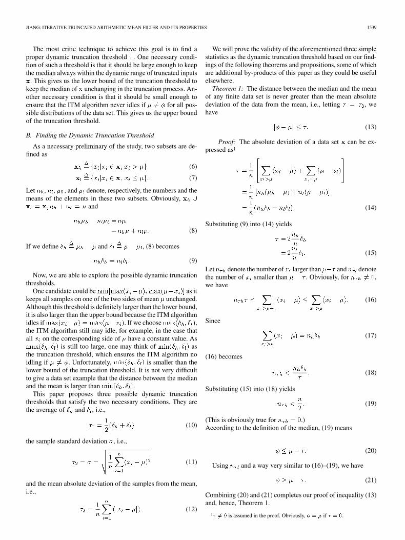
Although the ITM1 filter does not own Property 2, it blurs thestep edge lighter than the mean filter with just a few iterations.Fig. 2(a) shows a step edge profile. The filter size of

is applied. After the first iteration, the outputs ofthe ITM2 filter are the same as those of the median filter. Thediamond and circle marked lines are, respectively, the outputsof the mean filter and the ITM1 filter after only five iterations.

Although the ITM filters do not preserve other smooth edges,they produce much lighter blur effect than the mean filter. Asmooth edge profile is modeled by a logsig function

, whose smoothness is controlled by . Theprofile approaches a step function if and approaches avery flat slope function or almost a constant if . Fig. 2(b)shows that blurs the edge much lighter than the mean filterand is very close to the median filter.

In addition to edge preservation, another apparent property ofthe ITM filters is that they preserve the homogeneous area of theimage. i.e., , if , .

Property 3: The ITM filters are invariant to scale and bias,i.e., if , , we have

(40)

(41)

where and are two constants. The proof is trivial and, hence,omitted.

Property 4: The ITM2 filter with any number of iterationsremoves impulses from homogeneous area , i.e.,

forfor

(42)where , and and are the numbers of elementsin sets and , respectively.

Proof: If , , and , all pixelsare out of the truncation bound, and all pixels

Fig. 2. Profile outputs of the median, mean, ITM1, and ITM2 filters of size� � �� after five iterations for the (a) step edge and (b) smooth edge.

are within it from the first iteration of the filter. Hence, ITM2filter outputs from the first iteration of the filter. Thiscompletes the proof.

IV. EXPERIMENTAL STUDIES

No parameter of the proposed filter is optimized for a specificdata set or noise distribution. The same parameters are appliedto the ITM filters throughout all experiments. The stopping cri-terion of the ITM algorithm is fixed as

and is fixed for theITM2 filter. Better filtering performances than those shown inthis paper will be obtained if the aforementioned parameters areadjusted for different data sets. All noise applied in this paperhas independent and identically distributed and zero mean. Thestandard deviation of Gaussian noise is denoted by . Six setsof experiments are reported here.

The first two sets of experiments test the filters’ noise attenu-ation capability in a homogeneous region, and the next two setstest the filters’ overall performance in image structure preserva-tion and noise attenuation. The ITM filters are compared withthe mean, median, T [19], [20], and MEM [21], [22] filters.The mean absolute error (MAE) over 100 000 independent out-puts is used as the performance indicator for synthetic data,and the mean-square error (MSE) is used for real images. Al-though some T filters with adaptive -values were proposed[24], [29], none of them outperforms an -fixed T filter aver-agely over the experiments. Thus, is chosen as the


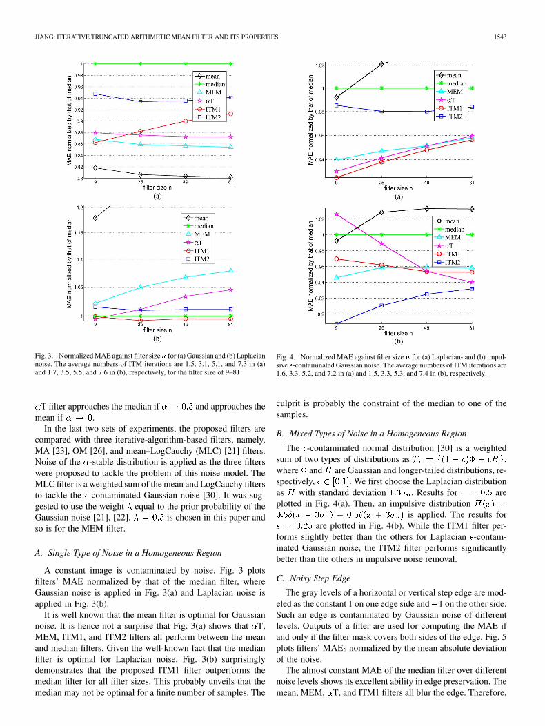
Fig. 3. Normalized MAE against filter size� for (a) Gaussian and (b) Laplaciannoise. The average numbers of ITM iterations are 1.5, 3.1, 5.1, and 7.3 in (a)and 1.7, 3.5, 5.5, and 7.6 in (b), respectively, for the filter size of 9–81.

T filter approaches the median if and approaches themean if .

In the last two sets of experiments, the proposed filters arecompared with three iterative-algorithm-based filters, namely,MA [23], OM [26], and mean–LogCauchy (MLC) [21] filters.Noise of the -stable distribution is applied as the three filterswere proposed to tackle the problem of this noise model. TheMLC filter is a weighted sum of the mean and LogCauchy filtersto tackle the -contaminated Gaussian noise [30]. It was sug-gested to use the weight equal to the prior probability of theGaussian noise [21], [22]. is chosen in this paper andso is for the MEM filter.

A. Single Type of Noise in a Homogeneous Region

A constant image is contaminated by noise. Fig. 3 plotsfilters’ MAE normalized by that of the median filter, whereGaussian noise is applied in Fig. 3(a) and Laplacian noise isapplied in Fig. 3(b).

It is well known that the mean filter is optimal for Gaussiannoise. It is hence not a surprise that Fig. 3(a) shows that T,MEM, ITM1, and ITM2 filters all perform between the meanand median filters. Given the well-known fact that the medianfilter is optimal for Laplacian noise, Fig. 3(b) surprisinglydemonstrates that the proposed ITM1 filter outperforms themedian filter for all filter sizes. This probably unveils that themedian may not be optimal for a finite number of samples. The

Fig. 4. Normalized MAE against filter size � for (a) Laplacian- and (b) impul-sive �-contaminated Gaussian noise. The average numbers of ITM iterations are1.6, 3.3, 5.2, and 7.2 in (a) and 1.5, 3.3, 5.3, and 7.4 in (b), respectively.

culprit is probably the constraint of the median to one of thesamples.

B. Mixed Types of Noise in a Homogeneous Region

The -contaminated normal distribution [30] is a weightedsum of two types of distributions as ,where and are Gaussian and longer-tailed distributions, re-spectively, . We first choose the Laplacian distributionas with standard deviation . Results for areplotted in Fig. 4(a). Then, an impulsive distribution

is applied. The results forare plotted in Fig. 4(b). While the ITM1 filter per-

forms slightly better than the others for Laplacian -contam-inated Gaussian noise, the ITM2 filter performs significantlybetter than the others in impulsive noise removal.

C. Noisy Step Edge

The gray levels of a horizontal or vertical step edge are mod-eled as the constant 1 on one edge side and 1 on the other side.Such an edge is contaminated by Gaussian noise of differentlevels. Outputs of a filter are used for computing the MAE ifand only if the filter mask covers both sides of the edge. Fig. 5plots filters’ MAEs normalized by the mean absolute deviationof the noise.

The almost constant MAE of the median filter over differentnoise levels shows its excellent ability in edge preservation. Themean, MEM, T, and ITM1 filters all blur the edge. Therefore,


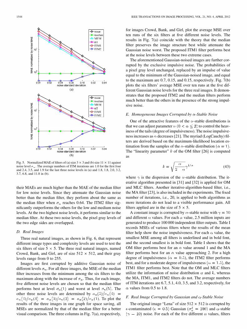
Fig. 5. Normalized MAE of filters of (a) size 3� 3 and (b) size 11� 11 againstnoise level � . The average numbers of ITM iterations are 1.0 for the first fourand 2.4, 3.5, and 1.9 for the last three noise levels in (a) and 1.8, 1.8, 2.0, 3.2,3.7, 6.8, and 11.8 in (b).

their MAEs are much higher than the MAE of the median filterfor low noise levels. Since they attenuate the Gaussian noisebetter than the median filter, they perform about the same asthe median filter when reaches 0.64. The ITM2 filter sig-nificantly outperforms the others for the low and medium noiselevels. At the two highest noise levels, it performs similar to themedian filter. At these two noise levels, the pixel gray levels ofthe two edge sides are overlapped.

D. Real Images

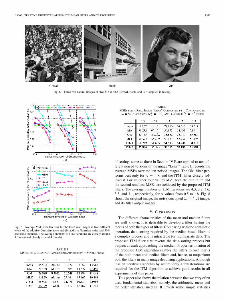
Three real natural images, as shown in Fig. 6, that representdifferent image types and complexity levels are used to test thesix filters of size 5 5. The three real natural images, namedCrowd, Bank, and Girl, are of size 512 512, and their graylevels range from 0 to 255.

Images are first corrupted by additive Gaussian noise ofdifferent levels . For all three images, the MSE of the medianfilter increases from the minimum among the six filters to themaximum along with the increase of . Thus, for each image,five different noise levels are chosen so that the median filterperforms best at level and worst at level . Theother three noise levels are determined by

. To plot theresults of the three images in one graph for space saving, allMSEs are normalized by that of the median filter for a bettervisual comparison. The three columns in Fig. 7(a), respectively,

for images Crowd, Bank, and Girl, plot the average MSE overten runs of the six filters at five different noise levels. Theresults in Fig. 7(a) coincide with the theory that the medianfilter preserves the image structure best while attenuate theGaussian noise worst. The proposed ITM1 filter performs bestat the noise levels between these two extreme cases.

The aforementioned Gaussian-noised images are further cor-rupted by the exclusive impulsive noise. The probabilities ofa pixel gray level unchanged, replaced by an impulse of valueequal to the minimum of the Gaussian-noised image, and equalto the maximum are 0.7, 0.15, and 0.15, respectively. Fig. 7(b)plots the six filters’ average MSE over ten runs at the five dif-ferent Gaussian noise levels for the three real images. It demon-strates that the proposed ITM2 and the median filters performmuch better than the others in the presence of the strong impul-sive noise.

E. Homogeneous Images Corrupted by -Stable Noise

One of the attractive features of the -stable distributions isthat we can adjust parameter to control the heav-iness of the tails (degree of impulsiveness). The noise impulsive-ness increases as decreases [21]. The myriad (LogCauchy) fil-ters are derived based on the maximum-likelihood location es-timation from the samples of the -stable distribution .The “linearity parameter” of the OM filter [26] is computedas

(43)

where is the dispersion of the -stable distribution. The it-erative algorithm presented in [31] and [32] is applied for OMand MLC filters. Another iterative-algorithm-based filter, i.e.,the MA filter [23], is also included in the experiments. The fixednumber of iterations, i.e., 20, is applied to both algorithms asmore iterations do not lead to a visible performance gain. Allfilters applied are in the size of 5 5.

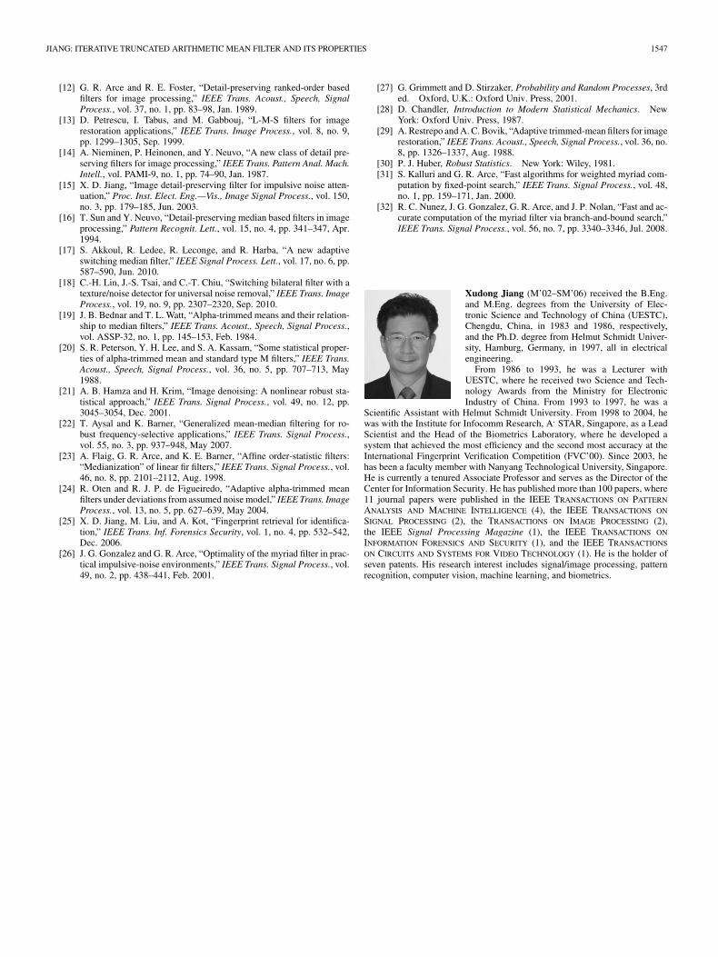
A constant image is corrupted by -stable noise withand different values. For each value, 2.5 million inputs aregenerated to produce 100 000 independent filter outputs. Table Irecords MSEs of various filters where the results of the meanfilter help show the noise impulsiveness. For each value, thesmallest MSE among all filters is underlined and in bold font,and the second smallest is in bold font. Table I shows that theOM filter performs best for an value around 1 and the MAfilter performs best for an value approaching 2. For a highdegree of impulsiveness , the ITM2 filter performsbest, and for a moderate degree of impulsiveness , theITM1 filter performs best. Note that the OM and MLC filtersutilize the information of noise distribution and , whereasthe MA, ITM1, and ITM2 filters do not. The average numbersof ITM iterations are 6.7, 5.1, 4.0, 3.5, and 3.2, respectively, for

values from 0.5 to 1.8.

F. Real Image Corrupted by Gaussian and -Stable Noise

The original image “Lena” of size 512 512 is corrupted by-contaminated Gaussian and -stable

noise. For each of the five different values, filters


Fig. 6. Three real natural images of size 512 � 512 (Crowd, Bank, and Girl) applied in testing.

Fig. 7. Average MSE over ten runs for the three real images at five differentlevels of (a) additive Gaussian noise and (b) additive Gaussian noise and 30%exclusive impulses. The average numbers of ITM iterations are closely around3.3 in (a) and closely around 4.5 in (b).

TABLE IMSES FOR A CONSTANT IMAGE CONTAMINATED BY �-STABLE NOISE

TABLE IIMSES FOR A REAL IMAGE “LENA” CORRUPTED BY �-CONTAMINATED

�� GAUSSIAN �� AND �-STABLE �� NOISE

of settings same as those in Section IV-E are applied to ten dif-ferent noised versions of the image “Lena.” Table II records theaverage MSEs over the ten noised images. The OM filter per-forms best only for , and the ITM1 filter closely fol-lows it. For all other four values of , both the minimum andthe second smallest MSEs are achieved by the proposed ITMfilters. The average numbers of ITM iterations are 4.3, 3.8, 3.6,3.3, and 3.1, respectively, for values from 0.5 to 1.8. Fig. 8shows the original image, the noise-corrupted image,and its filter output images.

V. CONCLUSION

The different characteristics of the mean and median filtersare well known. It is desirable to develop a filter having themerits of both the types of filters. Comparing with the arithmeticoperation, data sorting required by the median-based filters isa complex process and is intractable for multivariate data. Theproposed ITM filter circumvents the data-sorting process butoutputs a result approaching the median. Proper termination ofthe proposed ITM algorithm enables the filters to own meritsof the both mean and median filters and, hence, to outperformboth the filters in many image denoising applications. Althoughit is an iterative algorithm by nature, only a few iterations arerequired for the ITM algorithm to achieve good results in allexperiments of this paper.

This paper also shows the relation between the two very oftenused fundamental statistics, namely, the arithmetic mean andthe order statistical median. It unveils some simple statistics


Fig. 8. Filtering results of the noise-corrupted image “Lena” of size 512� 512. (a) Original image. (b) Corrupted image by �-contaminated �� Gaussian�� and �-stable �� noise. Outputs of (c) MA, (d) OM, (e) MLC, and (f) ITM1 filters of size 5 � 5.

of a finite data set as the upper bounds of the deviation of themedian from the mean. The tightest upper bound discoveredin this paper is applied as the truncation threshold, aiming atthe smallest number of iterations, which, however, may notdeliver the best filtering performance. Some general stoppingcriteria are suggested, although a better one for some specificapplications is possible. Properties of the proposed ITM1 andITM2 filters are theoretically analyzed and experimentallyverified.

Comprehensive simulation results with a fixed parameter setthroughout all experiments demonstrate the superiority and flex-ibility of the proposed filters. The significant difference of theITM filter from the median, MEM, T, MTM, and MA filtersis that it circumvents the data-sorting operation. Different fromthe myriad and MLC filters, the ITM filters are not distribu-tion-model specific and, hence, have greater application scope.One possible further development is to explore some proper cri-teria, based on which the filter can automatically switch betweenITM1 and ITM2. Better filtering performance can be certainlyexpected with a proper switch mechanism because the ITM1filter performs better in the smooth area with short-tailed andlight long-tailed noise and the ITM2 filter preserves the imagestructure better and is more powerful in removing heavy impul-sive noise.

REFERENCES

[1] A. Burian and P. Kuosmanen, “Tuning the smoothness of the recur-sive median filter,” IEEE Trans. Signal Process., vol. 50, no. 7, pp.1631–1639, Jul. 2002.

[2] I. Pitas and A. N. Venetsanopoulos, “Order statistics in digital imageprocessing,” Proc. IEEE, vol. 80, no. 12, pp. 1893–1921, Dec. 1992.

[3] R. Yang, L. Yin, M. Gabbouj, J. Astola, and Y. Neuvo, “Optimalweighted median filtering under structural constraints,” IEEE Trans.Signal Process., vol. 43, no. 3, pp. 591–604, Mar. 1995.

[4] L. Yin, R. Yang, M. Gabbouj, and Y. Neuvo, “Weighted median filters:A tutorial,” IEEE Trans. Circuits Syst. II, Analog Digit. Signal Process.,vol. 43, no. 3, pp. 157–192, Mar. 1996.

[5] S. Hoyos, Y. Li, J. Bacca, and G. R. Arce, “Weighted median filters ad-mitting complex-valued weights and their optimization,” IEEE Trans.Signal Process., vol. 52, no. 10, pp. 2776–2787, Oct. 2004.

[6] D. Charalampidis, “Steerable weighted median filters,” IEEE Trans.Image Process., vol. 19, no. 4, pp. 882–894, Apr. 2010.

[7] R. C. Hardie and C. G. Boncelet, “LUM filter: A class ofrank-order-based filters for smoothing and sharpening,” IEEE Trans.Signal Process., vol. 41, no. 3, pp. 1061–1076, Mar. 1993.

[8] Y. Nie and K. E. Barner, “Fuzzy rank LUM filters,” IEEE Trans. ImageProcess., vol. 15, no. 12, pp. 3636–3654, Dec. 2006.

[9] K. E. Barner, A. Flaig, and G. R. Arce, “Fuzzy time–rank relations andorder statistics,” IEEE Signal Process. Lett., vol. 5, no. 10, pp. 252–255,Oct. 1998.

[10] K. E. Barner, Y. Nie, and W. An, “Fuzzy ordering theory and its usein filter generalization,” EURASIP J. Appl. Signal Process., vol. 2001,no. 4, pp. 206–218, 2001.

[11] R. C. Hardie and K. E. Barner, “Rank conditioned rank selection filtersfor signal restoration,” IEEE Trans. Image Process., vol. 3, no. 2, pp.192–206, Mar. 1994.


[12] G. R. Arce and R. E. Foster, “Detail-preserving ranked-order basedfilters for image processing,” IEEE Trans. Acoust., Speech, SignalProcess., vol. 37, no. 1, pp. 83–98, Jan. 1989.

[13] D. Petrescu, I. Tabus, and M. Gabbouj, “L-M-S filters for imagerestoration applications,” IEEE Trans. Image Process., vol. 8, no. 9,pp. 1299–1305, Sep. 1999.

[14] A. Nieminen, P. Heinonen, and Y. Neuvo, “A new class of detail pre-serving filters for image processing,” IEEE Trans. Pattern Anal. Mach.Intell., vol. PAMI-9, no. 1, pp. 74–90, Jan. 1987.

[15] X. D. Jiang, “Image detail-preserving filter for impulsive noise atten-uation,” Proc. Inst. Elect. Eng.—Vis., Image Signal Process., vol. 150,no. 3, pp. 179–185, Jun. 2003.

[16] T. Sun and Y. Neuvo, “Detail-preserving median based filters in imageprocessing,” Pattern Recognit. Lett., vol. 15, no. 4, pp. 341–347, Apr.1994.

[17] S. Akkoul, R. Ledee, R. Leconge, and R. Harba, “A new adaptiveswitching median filter,” IEEE Signal Process. Lett., vol. 17, no. 6, pp.587–590, Jun. 2010.

[18] C.-H. Lin, J.-S. Tsai, and C.-T. Chiu, “Switching bilateral filter with atexture/noise detector for universal noise removal,” IEEE Trans. ImageProcess., vol. 19, no. 9, pp. 2307–2320, Sep. 2010.

[19] J. B. Bednar and T. L. Watt, “Alpha-trimmed means and their relation-ship to median filters,” IEEE Trans. Acoust., Speech, Signal Process.,vol. ASSP-32, no. 1, pp. 145–153, Feb. 1984.

[20] S. R. Peterson, Y. H. Lee, and S. A. Kassam, “Some statistical proper-ties of alpha-trimmed mean and standard type M filters,” IEEE Trans.Acoust., Speech, Signal Process., vol. 36, no. 5, pp. 707–713, May1988.

[21] A. B. Hamza and H. Krim, “Image denoising: A nonlinear robust sta-tistical approach,” IEEE Trans. Signal Process., vol. 49, no. 12, pp.3045–3054, Dec. 2001.

[22] T. Aysal and K. Barner, “Generalized mean-median filtering for ro-bust frequency-selective applications,” IEEE Trans. Signal Process.,vol. 55, no. 3, pp. 937–948, May 2007.

[23] A. Flaig, G. R. Arce, and K. E. Barner, “Affine order-statistic filters:“Medianization” of linear fir filters,” IEEE Trans. Signal Process., vol.46, no. 8, pp. 2101–2112, Aug. 1998.

[24] R. Oten and R. J. P. de Figueiredo, “Adaptive alpha-trimmed meanfilters under deviations from assumed noise model,” IEEE Trans. ImageProcess., vol. 13, no. 5, pp. 627–639, May 2004.

[25] X. D. Jiang, M. Liu, and A. Kot, “Fingerprint retrieval for identifica-tion,” IEEE Trans. Inf. Forensics Security, vol. 1, no. 4, pp. 532–542,Dec. 2006.

[26] J. G. Gonzalez and G. R. Arce, “Optimality of the myriad filter in prac-tical impulsive-noise environments,” IEEE Trans. Signal Process., vol.49, no. 2, pp. 438–441, Feb. 2001.

[27] G. Grimmett and D. Stirzaker, Probability and Random Processes, 3rded. Oxford, U.K.: Oxford Univ. Press, 2001.

[28] D. Chandler, Introduction to Modern Statistical Mechanics. NewYork: Oxford Univ. Press, 1987.

[29] A. Restrepo and A. C. Bovik, “Adaptive trimmed-mean filters for imagerestoration,” IEEE Trans. Acoust., Speech, Signal Process., vol. 36, no.8, pp. 1326–1337, Aug. 1988.

[30] P. J. Huber, Robust Statistics. New York: Wiley, 1981.[31] S. Kalluri and G. R. Arce, “Fast algorithms for weighted myriad com-

putation by fixed-point search,” IEEE Trans. Signal Process., vol. 48,no. 1, pp. 159–171, Jan. 2000.

[32] R. C. Nunez, J. G. Gonzalez, G. R. Arce, and J. P. Nolan, “Fast and ac-curate computation of the myriad filter via branch-and-bound search,”IEEE Trans. Signal Process., vol. 56, no. 7, pp. 3340–3346, Jul. 2008.

Xudong Jiang (M’02–SM’06) received the B.Eng.and M.Eng. degrees from the University of Elec-tronic Science and Technology of China (UESTC),Chengdu, China, in 1983 and 1986, respectively,and the Ph.D. degree from Helmut Schmidt Univer-sity, Hamburg, Germany, in 1997, all in electricalengineering.

From 1986 to 1993, he was a Lecturer withUESTC, where he received two Science and Tech-nology Awards from the Ministry for ElectronicIndustry of China. From 1993 to 1997, he was a

Scientific Assistant with Helmut Schmidt University. From 1998 to 2004, hewas with the Institute for Infocomm Research, A STAR, Singapore, as a LeadScientist and the Head of the Biometrics Laboratory, where he developed asystem that achieved the most efficiency and the second most accuracy at theInternational Fingerprint Verification Competition (FVC’00). Since 2003, hehas been a faculty member with Nanyang Technological University, Singapore.He is currently a tenured Associate Professor and serves as the Director of theCenter for Information Security. He has published more than 100 papers, where11 journal papers were published in the IEEE TRANSACTIONS ON PATTERN

ANALYSIS AND MACHINE INTELLIGENCE (4), the IEEE TRANSACTIONS ON

SIGNAL PROCESSING (2), the TRANSACTIONS ON IMAGE PROCESSING (2),the IEEE Signal Processing Magazine (1), the IEEE TRANSACTIONS ON

INFORMATION FORENSICS AND SECURITY (1), and the IEEE TRANSACTIONS

ON CIRCUITS AND SYSTEMS FOR VIDEO TECHNOLOGY (1). He is the holder ofseven patents. His research interest includes signal/image processing, patternrecognition, computer vision, machine learning, and biometrics.

Documents

IEEE TRANSACTIONS ON IMAGE PROCESSING, VOL. … · Iterative Truncated Arithmetic Mean Filter and Its Properties Xudong Jiang, Senior Member, IEEE ... metic operations, which owns