IEEE TRANSACTIONS ON IMAGE PROCESSING 1 Automatic Liver Segmentation ... · IEEE TRANSACTIONS ON IMAGE PROCESSING 1 Automatic Liver Segmentation based on Shape Constraints and Deformable

IEEE TRANSACTIONS ON IMAGE PROCESSING 1

Automatic Liver Segmentation based on ShapeConstraints and Deformable Graph Cut in CT

ImagesGuodong Li #, Xinjian Chen #, Fei Shi, Weifang Zhu, Jie Tian*, Fellow, IEEE, Dehui Xiang*

Abstract—Liver segmentation is still a challenging task inmedical image processing area due to the complexity of theliver’s anatomy, low contrast with adjacent organs and presenceof pathologies. This investigation was used to develop andvalidate an automated method to segment livers in CT images.The proposed framework consists of three steps: preprocessing,initialization and segmentation. In the first step, statistical shapemodel is constructed based on principal component analysis andthe input image is smoothed using curvature anisotropic diffusionfiltering. In the second step, the mean shape model is movedby using thresholding and Euclidean distance transformation toobtain a coarse position in a test image, and then the initial meshis locally and iteratively deformed to the coarse boundary, whichis constrained to stay close to a subspace of shapes describingthe anatomical variability. Finally, in order to accurately detectthe liver surface, deformable graph cut was proposed, whicheffectively integrates the properties and inter-relationship of theinput images and initialized surface. The proposed method wasevaluated on 50 CT scan images, which are publicly available intwo databases Sliver07 and 3Dircadb. The experimental resultsshowed that the proposed method was effective and accurate fordetection of the liver surface.

Index Terms—Liver Segmentation, Principal Component Anal-ysis, Euclidean Distance Transformation, Deformable Graph Cut.

I. INTRODUCTION

L IVER cancer has been among the 6 most commoncancers and also a leading cause of cancer deaths

worldwide. In 2012, it was reported that about 782,000 newcases were diagnosed with liver cancer and about 745, 000people died from this disease worldwide [1]. Consequently,particular effort is being made in early diagnosis and therapy.Liver segmentation in medical images is very important toaccurately evaluate patient-specific liver anatomy for hepaticdisease diagnosis, function assessment and treatment decision-making. Computed Tomography (CT) is now well-establishedfor noninvasive diagnosis of hepatic disease due to recent

This work has been supported in part by the National Basic ResearchProgram of China (973 Program) under Grant 2014CB748600, and in partby the National Natural Science Foundation of China (NSFC) under Grant81371629,61401293,61401294,81401451,81401472, and part by Natural Sci-ence Foundation of the Jiangsu Higher Education of China under Grant14KJB510032. Asterisk indicates corresponding author. # indicates the authorscontributed equally.

Guodong Li and Jie Tian are with the Institute of Automation, ChineseAcademy of Sciences, Beijing 100190, China.

Dehui Xiang, Xinjian Chen, Fei Shi and Weifang Zhu are with the Schoolof Electronics and Information Engineering, Soochow University, Jiangsu215006, China (email: [email protected]).

(a) (b)

Fig. 1. Examples of the complex anatomical structures and large variationsof liver shapes. (a) A CT image slice of a healthy person in coronal view.(b) A CT image slice in axial view from one patient with liver cancer. Thenormal liver and its several neighboring organs share similar intensities whilethe liver parenchyma and pathological changes exhibit non-homogeneous graylevel.

technological advances in X-ray tubes, detectors, and recon-struction algorithms. On the other hand, the amount of dataproduced by high resolution CT scanners, as well as the timeneeded to review the resulting several thousand slices, has beencontinuously increasing, which makes it tedious and time-consuming for radiologists and physicians [2]. Semi-automaticor automatic liver segmentation are helpful and advisable inclinical applications. Recently, numerous methods have beenproposed to segment livers effectively and efficiently. Manyresearchers have provided publicly available datasets and/ororganized liver segmentation competitions to investigate thosecurrent segmentation algorithms [3].

Although CT images have been widely used in clinics, liversegmentation is still a challenging task in the medical imageprocessing field. As can be seen in Fig.1, there are severalspecial characteristics from the liver’s anatomical structure.First, there are several neighboring organs, e.g. muscles, heartand stomach, and they share similar intensities, which lead tolow contrast and blurred boundaries in CT images between theliver and its neighboring organs. Therefore, liver segmentationusing pixel based methods such as region growing may easilyleak to neighboring organs. Second, image artifacts, noiseand various pathologies, such as tumors often exist. Liversegmentation can be disturbed by different gray value intervalsbetween hepatic tissues and artifacts. To tackle these problems,shape priors are desirable and advisable, since they can help toseparate adjacent organs with similar intensities and preserveliver shape with non-homogeneous gray level [4]. However,liver shape modeling is not a trivial task. Anatomy of theliver varies largely from different health individuals both in


shape and size. Besides, tumors and other pathologies mayalso change anatomical structure of a liver.

In this paper, we introduce a coarse-to-fine approach for thesegmentation of the whole liver from CT images. To makethe method automatic, the liver first needs to be localized inthe image. This task is challenging due to inter-patient andinter-phase shape variability, liver pose and location variabilityin the abdomen, variation in reconstructed field-of-view (thereconstructed image may focus on the liver or may cover thewhole chest and abdomen). After successful liver initializationusing model adaptation method, liver shape can be adapted tothe coarse boundary. Due to the complexity of liver anatomy,influenced by adjacent organs and insufficiency of shape prior,it makes accurate segmentation difficult. The patient’s anatomyis accurately and more robustly segmented using the proposeddeformable graph cut in a narrow band, which is well suited forinter-patient and inter-phase shape variability. The proposeddeformable graph cut can reduce under-segmentation or over-segmentation of livers since shape constraints are integratedinto region cost and boundary cost of the traditional graph cut[5]–[7] in a narrow band of the initial shape.

II. RELATED WORK

In the last few decades, many approaches have been pro-posed for liver segmentation. A comprehensive review ofdifferent methods have been presented [3], [8]. Simple pixel-based methods [9]–[12] include global thresholding, regiongrowing, voxel classification, or edge detection. Zhou et al.[9] used a probabilistic model to estimate the initial spatiallocation and calculated the liver probability to automaticallysegment the liver from non-contrast X-ray Torso CT images.van Rikxoort et al. [10] estimated the probability that eachvoxel is part of the liver using a k-nearest-neighbor classifi-er and a multi-atlas registration procedure to automaticallydelineate the liver from CT images. Foruzan et al. [12]proposed an intensity analysis and anatomical informationbased method. The authors used an expectation maximization(EM) algorithm to compute statistical parameters of the liver’sintensity range, and combined a thresholding approach and ananatomical based rule to interactively differentiate the liverfrom its surrounding tissues. The region-growing based liversegmentation approaches [11], [13], [14] can obtain goodresults from contrast enhanced CT images but they are verysensitive to initial seeds. Overall, pixel-based methods canusually fail to automatically segment a liver due to noise,similar gray-value distribution with neighboring organs, etc.

In 1993, Cootes et al. [15] introduced active shape modelsto image segmentation. Typically, 3D point distribution model(PDM) based statistical shape models (SSMs) were used in[16]–[18] to automatically segment the liver from CT images.These approaches first build a statistical model from a trainingset of liver shapes. Each liver shape is represented by somecorresponding landmarks sampled on the surface in the train-ing stage. Lamecker et al. [16] applied a SSM based methodwith grey value profile model to segment livers. Kainmulleret al. [17] integrated SSMs to a free-form segmentationmethod. Zhang et al. [18] obtained a coarse liver shapes in

a test CT images using a generalized Hough transformationbased subspace initialization method, and then detected liverboundaries using optimal surface segmentation. The optimalsurface detection algorithm proposed by Li et al. [19] wasused to find a minimum-cost closed set in a vertex-weightedgraph using max-flow/min-cut algorithms [6]. Heimann andMeinzer [3] presented an overview of SSMs based methodsfor segmentation of medical images. Wang et al. [4] integrateda sparse shape composition model and a fast marching levelset method to achieve accurate segmentation of the hepaticparenchyma, portal veins, hepatic veins, and tumors simultane-ously. Subsequently, they employed a homotopy-based methodto solve the L1-norm optimization problem [20].

Graph cut was employed to segment liver automaticallysince it was introduced by Boykov et al. [5]–[7]. To dealwith the intense memory requirements and the supralineartime complexity for traditional graph cut, Lombaert et al.[21] introduced a multilevel banded graph cuts method forfast image segmentation. Xe et al. [22] used a graph cutsbased active contour method for image segmentation in anarrow band. Massoptier et al. [23] applied a graph-cutmethod initialized by an adaptive threshold to perform fullyautomatic liver segmentation in CT images. Beichel et al. [24]developed an interactive segmentation system which allowedthe user to manipulate liver volume by combining a graph cutssegmentation method and a three-dimensional virtual realitybased segmentation refinement approach. Linguraru et al.[25] employed a 3-D affine invariant shape parameterizationmethod to compare features of a set of closed 3-D surfacespoint-to-point correspondence to detect shape ambiguities onan initial segmentation of the liver and used a shape-drivengeodesic active contour method to segment the liver, followedby hepatic tumor segmentation using graph cut. Chen et al.[26] combined an oriented active appearance model with apseudo-3-D initialization strategy and shape constrained graphcuts to automatically segment livers. Song et al. [27] roughlysegmented the liver based on a kernel fuzzy C-means algorith-m with spatial information and the refined segmentation wasperformed based on the GrowCut algorithm. Tomoshige et al.[28] combined a level set based conditional statistical shapemodel and graph cuts segmentation based on the estimatedshape prior to automatic liver segmentation from non-contrastabdominal CT volumes.

As described above, SSM based methods are desirable andhelpful to automatically segment livers from complex CTimages. Such methods use landmarks to represent shape anddescribe shape variation in the training data sets, which aredifficult to account for in a specific target organ. Graph-based methods can be utilized to search for a global optimalsolution while foreground seeds and background seeds areoften needed traditionally. Therefore, our aim is to combinethe complementary strengths of these methods to automaticallyand robustly segment livers from CT images in this paper.Compared to previous graph cut methods [5]–[7], [21], [26],[28], the contributions of our method are as follows,• Model initialization is performed by the integration of

principal component analysis (PCA), Euclidean distancetransformation (EDT) and deformable adaptation of the


Shape Model

Training

Training Shape Mean Shape

Variation Modes

Moved Shape

Smoothing

Graph Construction

Deformable Graph

Min-Cut/Max-Flow

Original Image Enhanced Image

Initialized Shape

EDT

EDT

EDT

Segmented Liver

Distance Field

Distance FieldTarget Boundary

Translation

Thresholding Model Adaptation

Preprocessing Model Initialization

Deformable Graph Cut

QuadricDecimation

Laplacian Smoothing

Mesh Subdivision

Dense Mesh

Distance Field

3.

2. 1.

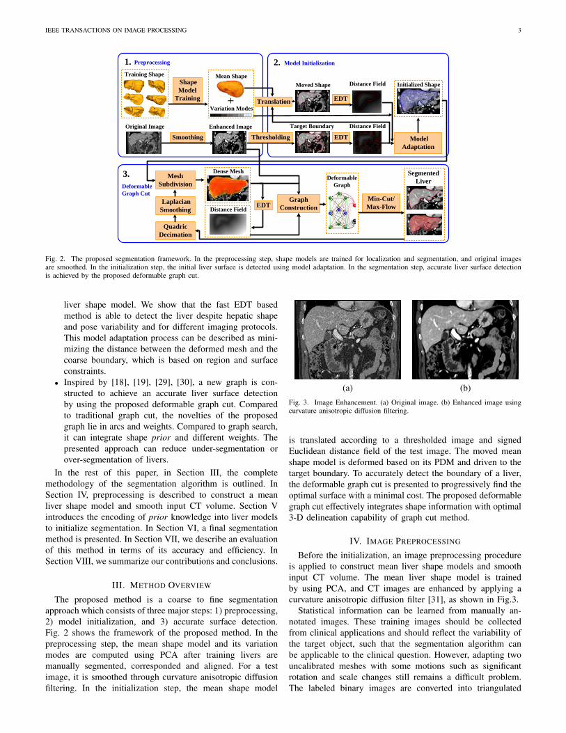
Fig. 2. The proposed segmentation framework. In the preprocessing step, shape models are trained for localization and segmentation, and original imagesare smoothed. In the initialization step, the initial liver surface is detected using model adaptation. In the segmentation step, accurate liver surface detectionis achieved by the proposed deformable graph cut.

liver shape model. We show that the fast EDT basedmethod is able to detect the liver despite hepatic shapeand pose variability and for different imaging protocols.This model adaptation process can be described as mini-mizing the distance between the deformed mesh and thecoarse boundary, which is based on region and surfaceconstraints.

• Inspired by [18], [19], [29], [30], a new graph is con-structed to achieve an accurate liver surface detectionby using the proposed deformable graph cut. Comparedto traditional graph cut, the novelties of the proposedgraph lie in arcs and weights. Compared to graph search,it can integrate shape prior and different weights. Thepresented approach can reduce under-segmentation orover-segmentation of livers.

In the rest of this paper, in Section III, the completemethodology of the segmentation algorithm is outlined. InSection IV, preprocessing is described to construct a meanliver shape model and smooth input CT volume. Section Vintroduces the encoding of prior knowledge into liver modelsto initialize segmentation. In Section VI, a final segmentationmethod is presented. In Section VII, we describe an evaluationof this method in terms of its accuracy and efficiency. InSection VIII, we summarize our contributions and conclusions.

III. METHOD OVERVIEW

The proposed method is a coarse to fine segmentationapproach which consists of three major steps: 1) preprocessing,2) model initialization, and 3) accurate surface detection.Fig. 2 shows the framework of the proposed method. In thepreprocessing step, the mean shape model and its variationmodes are computed using PCA after training livers aremanually segmented, corresponded and aligned. For a testimage, it is smoothed through curvature anisotropic diffusionfiltering. In the initialization step, the mean shape model

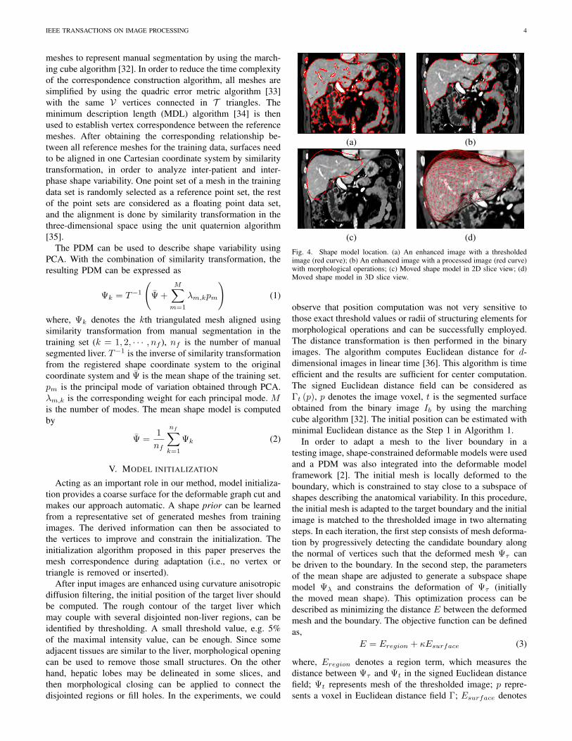
(a) (b)Fig. 3. Image Enhancement. (a) Original image. (b) Enhanced image usingcurvature anisotropic diffusion filtering.

is translated according to a thresholded image and signedEuclidean distance field of the test image. The moved meanshape model is deformed based on its PDM and driven to thetarget boundary. To accurately detect the boundary of a liver,the deformable graph cut is presented to progressively find theoptimal surface with a minimal cost. The proposed deformablegraph cut effectively integrates shape information with optimal3-D delineation capability of graph cut method.

IV. IMAGE PREPROCESSING

Before the initialization, an image preprocessing procedureis applied to construct mean liver shape models and smoothinput CT volume. The mean liver shape model is trainedby using PCA, and CT images are enhanced by applying acurvature anisotropic diffusion filter [31], as shown in Fig.3.

Statistical information can be learned from manually an-notated images. These training images should be collectedfrom clinical applications and should reflect the variability ofthe target object, such that the segmentation algorithm canbe applicable to the clinical question. However, adapting twouncalibrated meshes with some motions such as significantrotation and scale changes still remains a difficult problem.The labeled binary images are converted into triangulated


meshes to represent manual segmentation by using the march-ing cube algorithm [32]. In order to reduce the time complexityof the correspondence construction algorithm, all meshes aresimplified by using the quadric error metric algorithm [33]with the same V vertices connected in T triangles. Theminimum description length (MDL) algorithm [34] is thenused to establish vertex correspondence between the referencemeshes. After obtaining the corresponding relationship be-tween all reference meshes for the training data, surfaces needto be aligned in one Cartesian coordinate system by similaritytransformation, in order to analyze inter-patient and inter-phase shape variability. One point set of a mesh in the trainingdata set is randomly selected as a reference point set, the restof the point sets are considered as a floating point data set,and the alignment is done by similarity transformation in thethree-dimensional space using the unit quaternion algorithm[35].

The PDM can be used to describe shape variability usingPCA. With the combination of similarity transformation, theresulting PDM can be expressed as

Ψk = T−1

(Ψ +

M∑m=1

λm,kpm

)(1)

where, Ψk denotes the kth triangulated mesh aligned usingsimilarity transformation from manual segmentation in thetraining set (k = 1, 2, · · · , nf ), nf is the number of manualsegmented liver. T−1 is the inverse of similarity transformationfrom the registered shape coordinate system to the originalcoordinate system and Ψ is the mean shape of the training set.pm is the principal mode of variation obtained through PCA.λm,k is the corresponding weight for each principal mode. Mis the number of modes. The mean shape model is computedby

Ψ =1

nf

nf∑k=1

Ψk (2)

V. MODEL INITIALIZATION

Acting as an important role in our method, model initializa-tion provides a coarse surface for the deformable graph cut andmakes our approach automatic. A shape prior can be learnedfrom a representative set of generated meshes from trainingimages. The derived information can then be associated tothe vertices to improve and constrain the initialization. Theinitialization algorithm proposed in this paper preserves themesh correspondence during adaptation (i.e., no vertex ortriangle is removed or inserted).

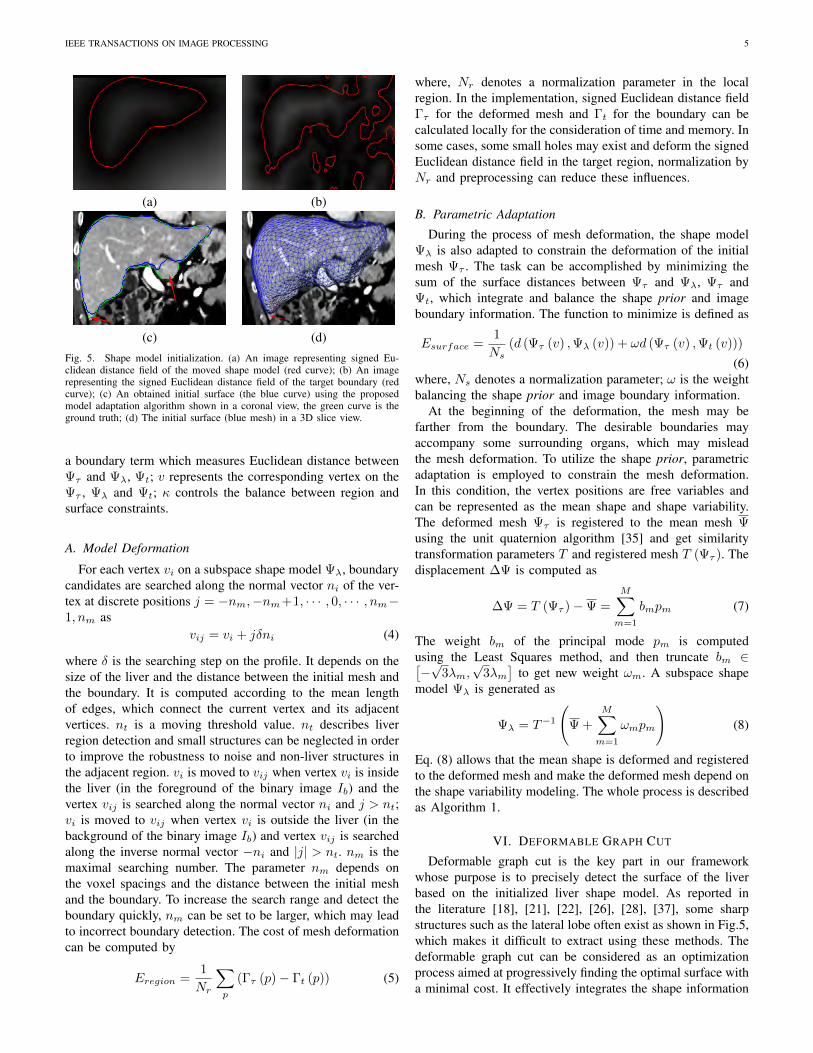
After input images are enhanced using curvature anisotropicdiffusion filtering, the initial position of the target liver shouldbe computed. The rough contour of the target liver whichmay couple with several disjointed non-liver regions, can beidentified by thresholding. A small threshold value, e.g. 5%of the maximal intensity value, can be enough. Since someadjacent tissues are similar to the liver, morphological openingcan be used to remove those small structures. On the otherhand, hepatic lobes may be delineated in some slices, andthen morphological closing can be applied to connect thedisjointed regions or fill holes. In the experiments, we could

(a) (b)

(c) (d)Fig. 4. Shape model location. (a) An enhanced image with a thresholdedimage (red curve); (b) An enhanced image with a processed image (red curve)with morphological operations; (c) Moved shape model in 2D slice view; (d)Moved shape model in 3D slice view.

observe that position computation was not very sensitive tothose exact threshold values or radii of structuring elements formorphological operations and can be successfully employed.The distance transformation is then performed in the binaryimages. The algorithm computes Euclidean distance for d-dimensional images in linear time [36]. This algorithm is timeefficient and the results are sufficient for center computation.The signed Euclidean distance field can be considered asΓt (p), p denotes the image voxel, t is the segmented surfaceobtained from the binary image Ib by using the marchingcube algorithm [32]. The initial position can be estimated withminimal Euclidean distance as the Step 1 in Algorithm 1.

In order to adapt a mesh to the liver boundary in atesting image, shape-constrained deformable models were usedand a PDM was also integrated into the deformable modelframework [2]. The initial mesh is locally deformed to theboundary, which is constrained to stay close to a subspace ofshapes describing the anatomical variability. In this procedure,the initial mesh is adapted to the target boundary and the initialimage is matched to the thresholded image in two alternatingsteps. In each iteration, the first step consists of mesh deforma-tion by progressively detecting the candidate boundary alongthe normal of vertices such that the deformed mesh Ψτ canbe driven to the boundary. In the second step, the parametersof the mean shape are adjusted to generate a subspace shapemodel Ψλ and constrains the deformation of Ψτ (initiallythe moved mean shape). This optimization process can bedescribed as minimizing the distance E between the deformedmesh and the boundary. The objective function can be definedas,

E = Eregion + κEsurface (3)

where, Eregion denotes a region term, which measures thedistance between Ψτ and Ψt in the signed Euclidean distancefield; Ψt represents mesh of the thresholded image; p repre-sents a voxel in Euclidean distance field Γ; Esurface denotes


(a) (b)

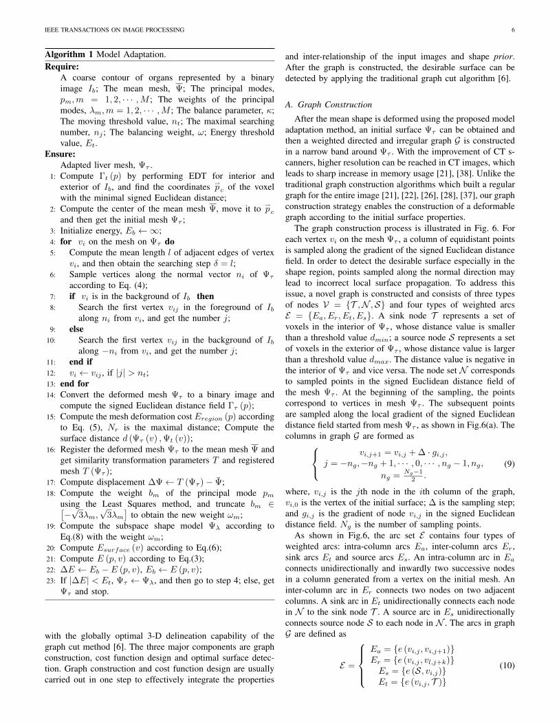
(c) (d)Fig. 5. Shape model initialization. (a) An image representing signed Eu-clidean distance field of the moved shape model (red curve); (b) An imagerepresenting the signed Euclidean distance field of the target boundary (redcurve); (c) An obtained initial surface (the blue curve) using the proposedmodel adaptation algorithm shown in a coronal view, the green curve is theground truth; (d) The initial surface (blue mesh) in a 3D slice view.

a boundary term which measures Euclidean distance betweenΨτ and Ψλ, Ψt; v represents the corresponding vertex on theΨτ , Ψλ and Ψt; κ controls the balance between region andsurface constraints.

A. Model Deformation

For each vertex vi on a subspace shape model Ψλ, boundarycandidates are searched along the normal vector ni of the ver-tex at discrete positions j = −nm,−nm+1, · · · , 0, · · · , nm−1, nm as

vij = vi + jδni (4)

where δ is the searching step on the profile. It depends on thesize of the liver and the distance between the initial mesh andthe boundary. It is computed according to the mean lengthof edges, which connect the current vertex and its adjacentvertices. nt is a moving threshold value. nt describes liverregion detection and small structures can be neglected in orderto improve the robustness to noise and non-liver structures inthe adjacent region. vi is moved to vij when vertex vi is insidethe liver (in the foreground of the binary image Ib) and thevertex vij is searched along the normal vector ni and j > nt;vi is moved to vij when vertex vi is outside the liver (in thebackground of the binary image Ib) and vertex vij is searchedalong the inverse normal vector −ni and |j| > nt. nm is themaximal searching number. The parameter nm depends onthe voxel spacings and the distance between the initial meshand the boundary. To increase the search range and detect theboundary quickly, nm can be set to be larger, which may leadto incorrect boundary detection. The cost of mesh deformationcan be computed by

Eregion =1

Nr

∑p

(Γτ (p)− Γt (p)) (5)

where, Nr denotes a normalization parameter in the localregion. In the implementation, signed Euclidean distance fieldΓτ for the deformed mesh and Γt for the boundary can becalculated locally for the consideration of time and memory. Insome cases, some small holes may exist and deform the signedEuclidean distance field in the target region, normalization byNr and preprocessing can reduce these influences.

B. Parametric Adaptation

During the process of mesh deformation, the shape modelΨλ is also adapted to constrain the deformation of the initialmesh Ψτ . The task can be accomplished by minimizing thesum of the surface distances between Ψτ and Ψλ, Ψτ andΨt, which integrate and balance the shape prior and imageboundary information. The function to minimize is defined as

Esurface =1

Ns(d (Ψτ (v) ,Ψλ (v)) + ωd (Ψτ (v) ,Ψt (v)))

(6)where, Ns denotes a normalization parameter; ω is the weightbalancing the shape prior and image boundary information.

At the beginning of the deformation, the mesh may befarther from the boundary. The desirable boundaries mayaccompany some surrounding organs, which may misleadthe mesh deformation. To utilize the shape prior, parametricadaptation is employed to constrain the mesh deformation.In this condition, the vertex positions are free variables andcan be represented as the mean shape and shape variability.The deformed mesh Ψτ is registered to the mean mesh Ψusing the unit quaternion algorithm [35] and get similaritytransformation parameters T and registered mesh T (Ψτ ). Thedisplacement ∆Ψ is computed as

∆Ψ = T (Ψτ )−Ψ =M∑m=1

bmpm (7)

The weight bm of the principal mode pm is computedusing the Least Squares method, and then truncate bm ∈[−√

3λm,√

3λm]

to get new weight ωm. A subspace shapemodel Ψλ is generated as

Ψλ = T−1

(Ψ +

M∑m=1

ωmpm

)(8)

Eq. (8) allows that the mean shape is deformed and registeredto the deformed mesh and make the deformed mesh depend onthe shape variability modeling. The whole process is describedas Algorithm 1.

VI. DEFORMABLE GRAPH CUT

Deformable graph cut is the key part in our frameworkwhose purpose is to precisely detect the surface of the liverbased on the initialized liver shape model. As reported inthe literature [18], [21], [22], [26], [28], [37], some sharpstructures such as the lateral lobe often exist as shown in Fig.5,which makes it difficult to extract using these methods. Thedeformable graph cut can be considered as an optimizationprocess aimed at progressively finding the optimal surface witha minimal cost. It effectively integrates the shape information


Algorithm 1 Model Adaptation.Require:

A coarse contour of organs represented by a binaryimage Ib; The mean mesh, Ψ; The principal modes,pm,m = 1, 2, · · · ,M ; The weights of the principalmodes, λm,m = 1, 2, · · · ,M ; The balance parameter, κ;The moving threshold value, nt; The maximal searchingnumber, nj ; The balancing weight, ω; Energy thresholdvalue, Et.

Ensure:Adapted liver mesh, Ψτ .

1: Compute Γt (p) by performing EDT for interior andexterior of Ib, and find the coordinates ⇀

pc of the voxelwith the minimal signed Euclidean distance;

2: Compute the center of the mean mesh Ψ, move it to ⇀pc

and then get the initial mesh Ψτ ;3: Initialize energy, Eb ←∞;4: for vi on the mesh on Ψτ do5: Compute the mean length l of adjacent edges of vertex

vi, and then obtain the searching step δ = l;6: Sample vertices along the normal vector ni of Ψτ

according to Eq. (4);7: if vi is in the background of Ib then8: Search the first vertex vij in the foreground of Ib

along ni from vi, and get the number j;9: else

10: Search the first vertex vij in the background of Ibalong −ni from vi, and get the number j;

11: end if12: vi ← vij , if |j| > nt;13: end for14: Convert the deformed mesh Ψτ to a binary image and

compute the signed Euclidean distance field Γτ (p);15: Compute the mesh deformation cost Eregion (p) according

to Eq. (5), Nr is the maximal distance; Compute thesurface distance d (Ψτ (v) ,Ψt (v));

16: Register the deformed mesh Ψτ to the mean mesh Ψ andget similarity transformation parameters T and registeredmesh T (Ψτ );

17: Compute displacement ∆Ψ← T (Ψτ )− Ψ;18: Compute the weight bm of the principal mode pm

using the Least Squares method, and truncate bm ∈[−√

3λm,√

3λm]

to obtain the new weight ωm;19: Compute the subspace shape model Ψλ according to

Eq.(8) with the weight ωm;20: Compute Esurface (v) according to Eq.(6);21: Compute E (p, v) according to Eq.(3);22: ∆E ← Eb − E (p, v), Eb ← E (p, v);23: If |∆E| < Et, Ψτ ← Ψλ, and then go to step 4; else, get

Ψτ and stop.

with the globally optimal 3-D delineation capability of thegraph cut method [6]. The three major components are graphconstruction, cost function design and optimal surface detec-tion. Graph construction and cost function design are usuallycarried out in one step to effectively integrate the properties

and inter-relationship of the input images and shape prior.After the graph is constructed, the desirable surface can bedetected by applying the traditional graph cut algorithm [6].

A. Graph Construction

After the mean shape is deformed using the proposed modeladaptation method, an initial surface Ψτ can be obtained andthen a weighted directed and irregular graph G is constructedin a narrow band around Ψτ . With the improvement of CT s-canners, higher resolution can be reached in CT images, whichleads to sharp increase in memory usage [21], [38]. Unlike thetraditional graph construction algorithms which built a regulargraph for the entire image [21], [22], [26], [28], [37], our graphconstruction strategy enables the construction of a deformablegraph according to the initial surface properties.

The graph construction process is illustrated in Fig. 6. Foreach vertex vi on the mesh Ψτ , a column of equidistant pointsis sampled along the gradient of the signed Euclidean distancefield. In order to detect the desirable surface especially in theshape region, points sampled along the normal direction maylead to incorrect local surface propagation. To address thisissue, a novel graph is constructed and consists of three typesof nodes V = {T ,N ,S} and four types of weighted arcsE = {Ea, Er, Et, Es}. A sink node T represents a set ofvoxels in the interior of Ψτ , whose distance value is smallerthan a threshold value dmin; a source node S represents a setof voxels in the exterior of Ψτ , whose distance value is largerthan a threshold value dmax. The distance value is negative inthe interior of Ψτ and vice versa. The node set N correspondsto sampled points in the signed Euclidean distance field ofthe mesh Ψτ . At the beginning of the sampling, the pointscorrespond to vertices in mesh Ψτ . The subsequent pointsare sampled along the local gradient of the signed Euclideandistance field started from mesh Ψτ , as shown in Fig.6(a). Thecolumns in graph G are formed as

vi,j+1 = vi,j + ∆ · gi,j ,j = −ng,−ng + 1, · · · , 0, · · · , ng − 1, ng,

ng =Ng−1

2 .

(9)

where, vi,j is the jth node in the ith column of the graph,vi,0 is the vertex of the initial surface; ∆ is the sampling step;and gi,j is the gradient of node vi,j in the signed Euclideandistance field. Ng is the number of sampling points.

As shown in Fig.6, the arc set E contains four types ofweighted arcs: intra-column arcs Ea, inter-column arcs Er,sink arcs Et and source arcs Es. An intra-column arc in Eaconnects unidirectionally and inwardly two successive nodesin a column generated from a vertex on the initial mesh. Aninter-column arc in Er connects two nodes on two adjacentcolumns. A sink arc in Et unidirectionally connects each nodein N to the sink node T . A source arc in Es unidirectionallyconnects source node S to each node in N . The arcs in graphG are defined as

E =

Ea = {e (vi,j , vi,j+1)}Er = {e (vi,j , vl,j+k)}Es = {e (S, vi,j)}Et = {e (vi,j , T )}

(10)


(a)

: Node

: Inter-Column Arc

: Intra-Column Arc

Initial Surface Source Node

Sink Node

: Source Arc

: Sink ArcT

S

sE

TE

aE

rE

N

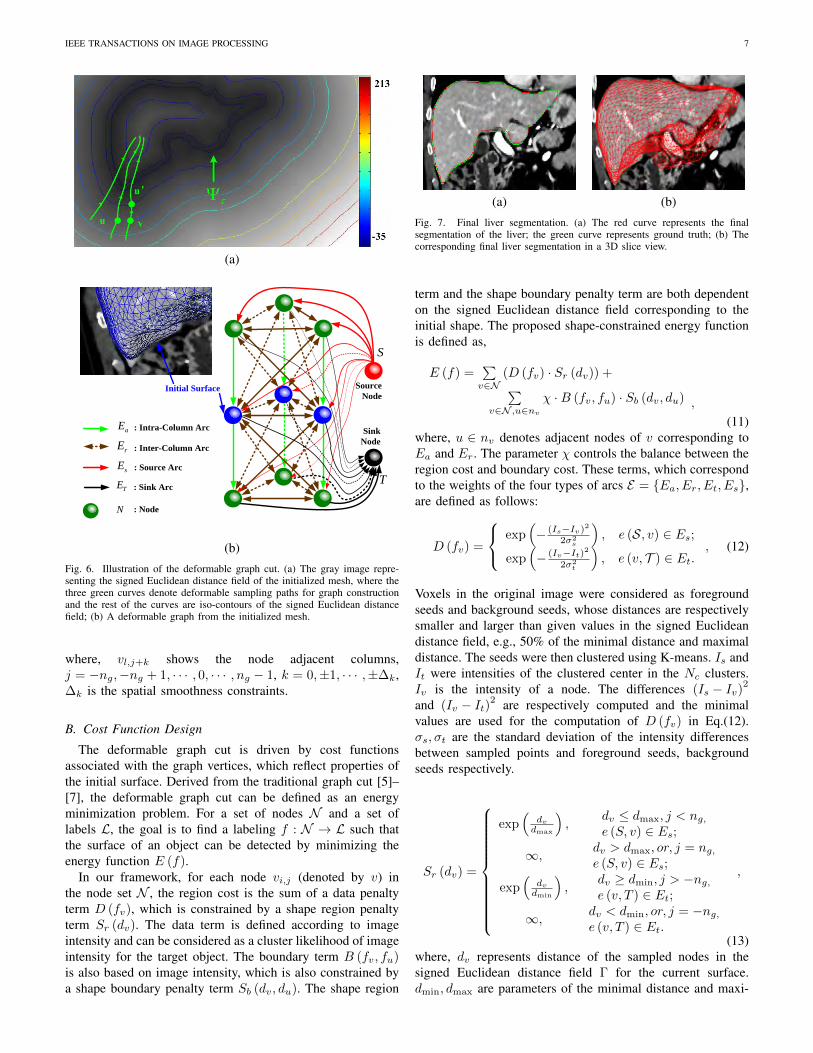
(b)Fig. 6. Illustration of the deformable graph cut. (a) The gray image repre-senting the signed Euclidean distance field of the initialized mesh, where thethree green curves denote deformable sampling paths for graph constructionand the rest of the curves are iso-contours of the signed Euclidean distancefield; (b) A deformable graph from the initialized mesh.

where, vl,j+k shows the node adjacent columns,j = −ng,−ng + 1, · · · , 0, · · · , ng − 1, k = 0,±1, · · · ,±∆k,∆k is the spatial smoothness constraints.

B. Cost Function Design

The deformable graph cut is driven by cost functionsassociated with the graph vertices, which reflect properties ofthe initial surface. Derived from the traditional graph cut [5]–[7], the deformable graph cut can be defined as an energyminimization problem. For a set of nodes N and a set oflabels L, the goal is to find a labeling f : N → L such thatthe surface of an object can be detected by minimizing theenergy function E (f).

In our framework, for each node vi,j (denoted by v) inthe node set N , the region cost is the sum of a data penaltyterm D (fv), which is constrained by a shape region penaltyterm Sr (dv). The data term is defined according to imageintensity and can be considered as a cluster likelihood of imageintensity for the target object. The boundary term B (fv, fu)is also based on image intensity, which is also constrained bya shape boundary penalty term Sb (dv, du). The shape region

(a) (b)Fig. 7. Final liver segmentation. (a) The red curve represents the finalsegmentation of the liver; the green curve represents ground truth; (b) Thecorresponding final liver segmentation in a 3D slice view.

term and the shape boundary penalty term are both dependenton the signed Euclidean distance field corresponding to theinitial shape. The proposed shape-constrained energy functionis defined as,

E (f) =∑v∈N

(D (fv) · Sr (dv)) +∑v∈N ,u∈nv

χ ·B (fv, fu) · Sb (dv, du) ,

(11)where, u ∈ nv denotes adjacent nodes of v corresponding toEa and Er. The parameter χ controls the balance between theregion cost and boundary cost. These terms, which correspondto the weights of the four types of arcs E = {Ea, Er, Et, Es},are defined as follows:

D (fv) =

exp(− (Is−Iv)2

2σ2s

), e (S, v) ∈ Es;

exp(− (Iv−It)2

2σ2t

), e (v, T ) ∈ Et.

, (12)

Voxels in the original image were considered as foregroundseeds and background seeds, whose distances are respectivelysmaller and larger than given values in the signed Euclideandistance field, e.g., 50% of the minimal distance and maximaldistance. The seeds were then clustered using K-means. Is andIt were intensities of the clustered center in the Nc clusters.Iv is the intensity of a node. The differences (Is − Iv)2and (Iv − It)2 are respectively computed and the minimalvalues are used for the computation of D (fv) in Eq.(12).σs, σt are the standard deviation of the intensity differencesbetween sampled points and foreground seeds, backgroundseeds respectively.

Sr (dv) =

exp(

dvdmax

),

dv ≤ dmax, j < ng,e (S, v) ∈ Es;

∞, dv > dmax, or, j = ng,e (S, v) ∈ Es;

exp(

dvdmin

),

dv ≥ dmin, j > −ng,e (v, T ) ∈ Et;

∞, dv < dmin, or, j = −ng,e (v, T ) ∈ Et.

,

(13)where, dv represents distance of the sampled nodes in thesigned Euclidean distance field Γ for the current surface.dmin, dmax are parameters of the minimal distance and maxi-


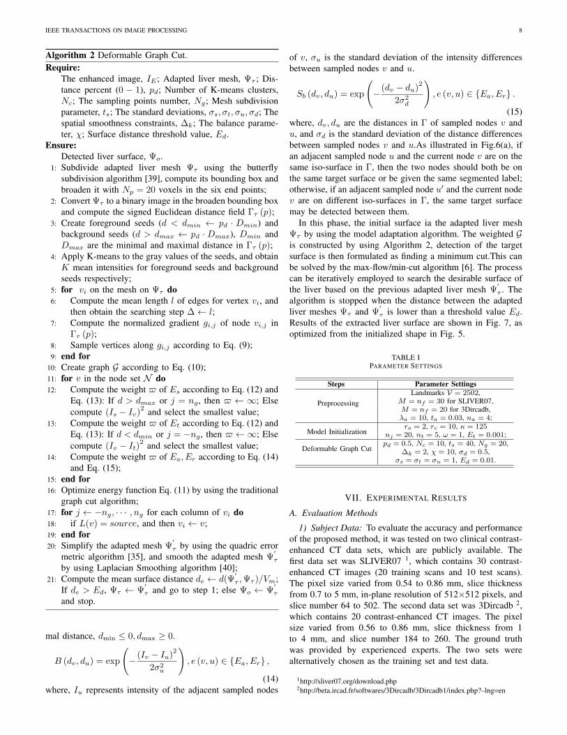
Algorithm 2 Deformable Graph Cut.Require:

The enhanced image, IE ; Adapted liver mesh, Ψτ ; Dis-tance percent (0 − 1), pd; Number of K-means clusters,Nc; The sampling points number, Ng; Mesh subdivisionparameter, ts; The standard deviations, σs, σt, σu, σd; Thespatial smoothness constraints, ∆k; The balance parame-ter, χ; Surface distance threshold value, Ed.

Ensure:Detected liver surface, Ψo.

1: Subdivide adapted liver mesh Ψτ using the butterflysubdivision algorithm [39], compute its bounding box andbroaden it with Np = 20 voxels in the six end points;

2: Convert Ψτ to a binary image in the broaden bounding boxand compute the signed Euclidean distance field Γτ (p);

3: Create foreground seeds (d < dmin ← pd · Dmin) andbackground seeds (d > dmax ← pd · Dmax), Dmin andDmax are the minimal and maximal distance in Γτ (p);

4: Apply K-means to the gray values of the seeds, and obtainK mean intensities for foreground seeds and backgroundseeds respectively;

5: for vi on the mesh on Ψτ do6: Compute the mean length l of edges for vertex vi, and

then obtain the searching step ∆← l;7: Compute the normalized gradient gi,j of node vi,j in

Γτ (p);8: Sample vertices along gi,j according to Eq. (9);9: end for

10: Create graph G according to Eq. (10);11: for v in the node set N do12: Compute the weight $ of Es according to Eq. (12) and

Eq. (13): If d > dmax or j = ng , then $ ← ∞; Elsecompute (Is − Iv)2 and select the smallest value;

13: Compute the weight $ of Et according to Eq. (12) andEq. (13): If d < dmin or j = −ng , then $ ←∞; Elsecompute (Iv − It)2 and select the smallest value;

14: Compute the weight $ of Ea, Er according to Eq. (14)and Eq. (15);

15: end for16: Optimize energy function Eq. (11) by using the traditional

graph cut algorithm;17: for j ← −ng, · · · , ng for each column of vi do18: if L(v) = source, and then vi ← v;19: end for20: Simplify the adapted mesh Ψ

′

τ by using the quadric errormetric algorithm [35], and smooth the adapted mesh Ψ

′

τ

by using Laplacian Smoothing algorithm [40];21: Compute the mean surface distance de ← d(Ψ

′

τ ,Ψτ )/Vm;If de > Ed, Ψτ ← Ψ

′

τ and go to step 1; else Ψo ← Ψ′

τ

and stop.

mal distance, dmin ≤ 0, dmax ≥ 0.

B (dv, du) = exp

(− (Iv − Iu)

2

2σ2u

), e (v, u) ∈ {Ea, Er} ,

(14)where, Iu represents intensity of the adjacent sampled nodes

of v, σu is the standard deviation of the intensity differencesbetween sampled nodes v and u.

Sb (dv, du) = exp

(− (dv − du)

2

2σ2d

), e (v, u) ∈ {Ea, Er} .

(15)where, dv, du are the distances in Γ of sampled nodes v andu, and σd is the standard deviation of the distance differencesbetween sampled nodes v and u.As illustrated in Fig.6(a), ifan adjacent sampled node u and the current node v are on thesame iso-surface in Γ, then the two nodes should both be onthe same target surface or be given the same segmented label;otherwise, if an adjacent sampled node u′ and the current nodev are on different iso-surfaces in Γ, the same target surfacemay be detected between them.

In this phase, the initial surface ia the adapted liver meshΨτ by using the model adaptation algorithm. The weighted Gis constructed by using Algorithm 2, detection of the targetsurface is then formulated as finding a minimum cut.This canbe solved by the max-flow/min-cut algorithm [6]. The processcan be iteratively employed to search the desirable surface ofthe liver based on the previous adapted liver mesh Ψ

′

τ . Thealgorithm is stopped when the distance between the adaptedliver meshes Ψτ and Ψ

′

τ is lower than a threshold value Ed.Results of the extracted liver surface are shown in Fig. 7, asoptimized from the initialized shape in Fig. 5.

TABLE IPARAMETER SETTINGS

Steps Parameter Settings

PreprocessingLandmarks V = 2502,

M = nf = 30 for SLIVER07,M = nf = 20 for 3Dircadb,λa = 10, ta = 0.03, na = 4;

Model Initializationro = 2, rc = 10, κ = 125

nj = 20, nt = 5, ω = 1, Et = 0.001;

Deformable Graph Cutpd = 0.5, Nc = 10, ts = 40, Ng = 20,

∆k = 2, χ = 10, σd = 0.5,σs = σt = σu = 1, Ed = 0.01.

VII. EXPERIMENTAL RESULTS

A. Evaluation Methods

1) Subject Data: To evaluate the accuracy and performanceof the proposed method, it was tested on two clinical contrast-enhanced CT data sets, which are publicly available. Thefirst data set was SLIVER07 1, which contains 30 contrast-enhanced CT images (20 training scans and 10 test scans).The pixel size varied from 0.54 to 0.86 mm, slice thicknessfrom 0.7 to 5 mm, in-plane resolution of 512×512 pixels, andslice number 64 to 502. The second data set was 3Dircadb 2,which contains 20 contrast-enhanced CT images. The pixelsize varied from 0.56 to 0.86 mm, slice thickness from 1to 4 mm, and slice number 184 to 260. The ground truthwas provided by experienced experts. The two sets werealternatively chosen as the training set and test data.

1http://sliver07.org/download.php2http://beta.ircad.fr/softwares/3Dircadb/3Dircadb1/index.php?–lng=en


2) Evaluation metrics: To quantitatively evaluate the per-formance of our proposed method, we compared the segmen-tation results with the ground truth according to the followingfive volume and surface based metrics [41]: volumetric over-lap error (VOE), signed relative volume difference (SRVD),average symmetric surface distance (ASD), root mean squaresymmetric surface distance (RMSD), and maximum symmet-ric surface distance (MSD). The volume and surface basedmetrics are given in percent and millimeters, respectively. Forall these evaluation metrics, the smaller the value is, the betterthe segmentation result.

3) Parameter Settings: In this section we will review de-tailed parameter settings for each step, where Table I listsall of the parameter settings. The number of landmarks andvertices of the initial shape model was V = 2502. Themean shape model of SLIVER07 was obtained from manualsegmentation by experienced experts and applied to 3Dircadbfor shape adaptation; The mean shape model of 3Dircadbwas obtained from manual segmentation by experienced ex-perts and applied to SLIVER07 for shape adaptation. Duringsmoothing by curvature anisotropic diffusion filtering, theconductance parameter λa was set at 10, the time step tawas around 0.03, and the number of iterations nawas typicallyset to 4. Apply morphological opening with round structuringelements (ro = 2) to remove small structures, and thenapply morphological closing with round structuring elements(rc = 10) to connect the disjointed regions or fill holes.κ = 125 typically can control the balance between regionand surface constraints. In our experiments, the voxel spacingrange was 0.54mm to 5.0 mm, nm = 20 and nt = 5 wereappropriate to efficiently deform the initial surface. For theconsideration of memory, the number of sampling points Ngwas set 40, since the initialized mesh was remeshed andsubdivided into dense meshes with about Vm = 40002 vertices(ts = 40) for the accurate detection of the target surface usingthe proposed deformable graph cut. The standard deviationsof the intensity σs, σt, σu were set at 1. The interval forthe standard deviation of the distance differences σd can be[0.1, 2], or typically 0.5. The balance parameter χ was set at10. The parameters described in this section were determinedexperimentally, but the detection was not very sensitive to theirexact values. The values described here were mainly motivatedby performance considerations. Our method was implementedin C++ and tested on a 32-bit desktop PC (3.1 GHz Core(TM)i5-3450 CPU and 4 GB RAM).

B. Validation Results

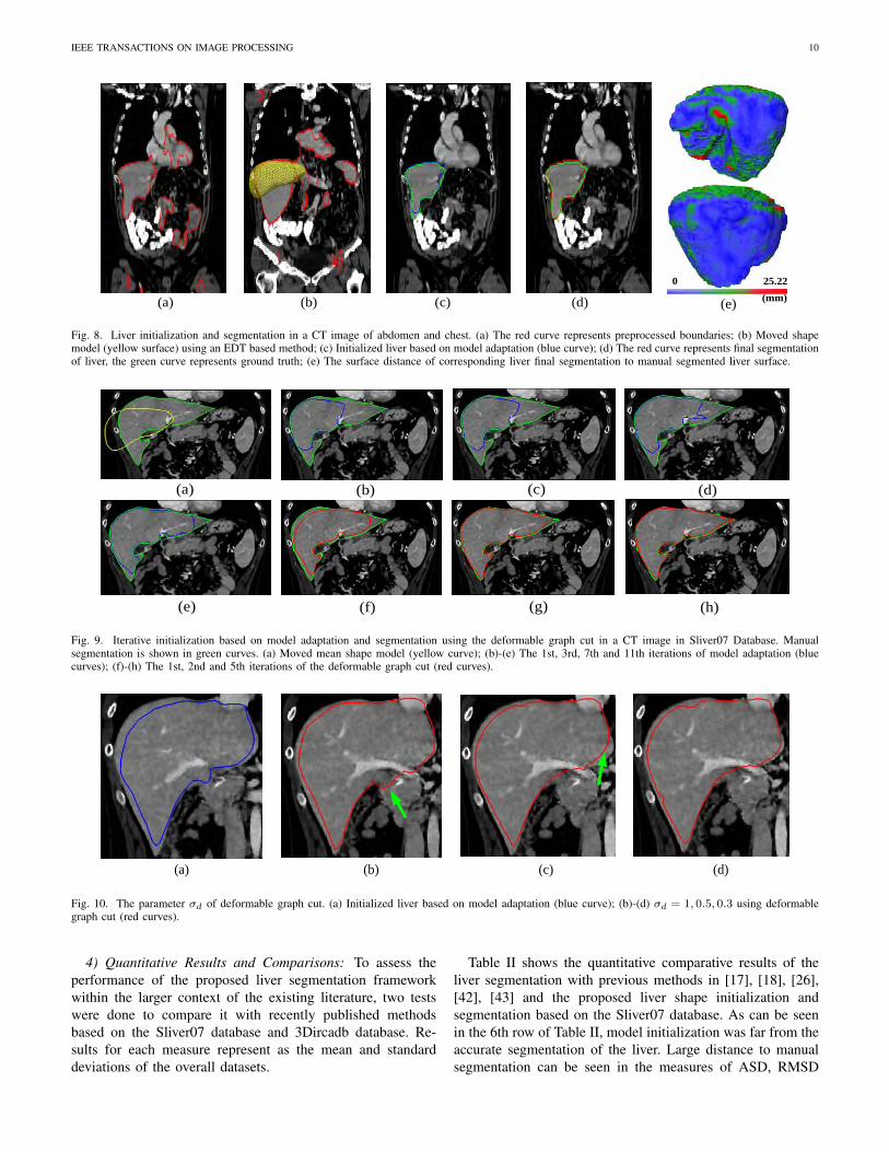
1) Case Study: During the experiments, the EDT basedmethod can be successfully applied to quickly localize thecoarse position of the liver. Fig.8 shows the whole processusing the proposed method in a CT image of the abdomenand chest in database Sliver07. The initialized surface and finalsurface are shown in Fig.8 (c) and (d) respectively.

Fig.9 (a)-(e) shows the mean shape model was iterativelyadapted to boundary of the liver. The green curves weremanual segmentation. The yellow curve in Fig.9 (a) is themean shape using the EDT based method. The surface was

far from the boundary of the liver and part of the model wasin the exterior of the liver. In the first iterations of modeladaptation, the shape model was adjusted to the boundary ofthe right hepatic lobe and then driven to the boundary of theleft hepatic lobe. However, it is difficult to detect boundaries ofsharp structures in both the right hepatic lobe and left hepaticlobe. On the one hand, model adaptation was constrained bya PDM from statistical shapes, which can not contain enoughshape variability of the livers; on the other hand, the modelwas adapted along its normal direction which was difficult toreach along those boundaries of the sharp structures.

Fig.9 (f)-(h) shows iterations using the deformable graphcut. To detect target boundaries of livers more accurately, theproposed deformable graph cut can detect target boundarieswith consideration of a region cost and boundary cost. As canbe seen in Fig.9 (f), the smooth surface was detected. Withthe integration of shape prior, the surface was progressivelyadapted to the target boundaries even if structures were sharp.This is because the mesh was remeshed and adjusted along adeformable distance field.

2) Effect of Different Parameters: Fig.10 shows the impactof shape σd of the deformable graph cut. Fig.9 (f)-(h) showssegmentation using different values σd = 1, 0.5, 0.3. As thevalue becomes larger, segmentation tends to include non-hepatic tissues with similar intensity, which often occursusing the traditional graph cut. As can be seen in this test,the proposed deformable graph cut can control the balancebetween the region and boundary by the integration of shapeprior more robustly, as illustrated in Fig.6(a).

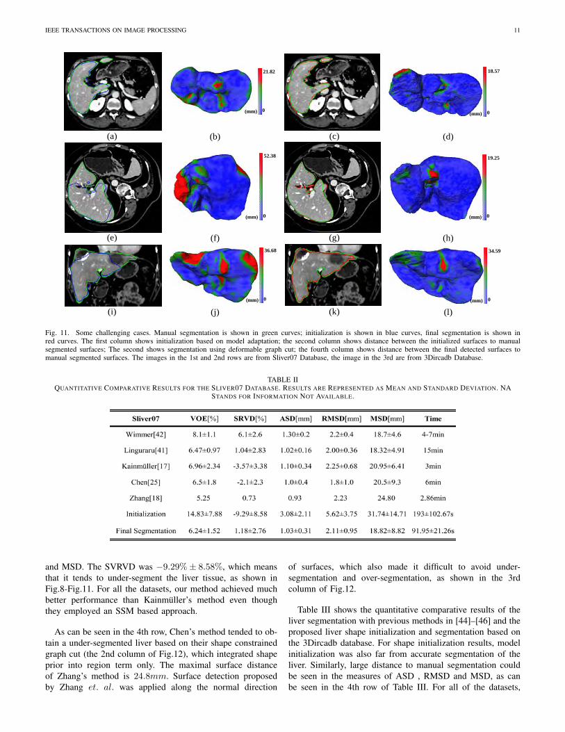
3) Challenging Cases: Fig.11 shows three challenging cas-es. The first row shows the segmentation of a CT imagefrom database 3Dircadb. There are 20 tumors in this CTimage. Besides, numerous sharp regions and divided lobesexist, as can be seen in Fig.11(a). As shown in Fig.11(a)-(b),model adaptation can be applied to reach most of the targetboundary. Some sharp structures were lost in the left lobeand near the vessel. The maximal distance to target boundarywas 21.82mm. With the help of deformable graph cut, thosesharp structures can be included, as shown in Fig.11(c)-(d).The maximal distance to the target boundary decreased to18.87mm. The second row shows the segmentation of a CTimage from database Sliver07. As shown in Fig.11(c), thesubject was laid on one side, which led to a large rotationwith regard to the mean shape model. Besides, a large gapalso exist. These two difficulties made it difficult to reachthe boundary of the left lobes for the shape model basedadaptation method, which led to 52.38mm of the maximaldistance to the target boundary. After the initial surface wasadapted using the deformable graph cut, the maximal distancewas decreased to 19.25mm, as shown in Fig.11(h). The thirdrow shows the segmentation of a CT image from database3Dircadb. There are 2 large tumors in this CT image. Ascan be seen in Fig.11(i), model adaptation stopped movingtowards the boundary of the liver. Large surface difference wasgenerated between the initialized liver and manual segmentedliver near the regions of the tumors as shown in Fig.11(j). Thedistance was then decreased to 34.59mm using the proposeddeformable graph cut as shown in Fig.11(l).


0 25.22

(a) (b) (c) (d) (e) (mm)

Fig. 8. Liver initialization and segmentation in a CT image of abdomen and chest. (a) The red curve represents preprocessed boundaries; (b) Moved shapemodel (yellow surface) using an EDT based method; (c) Initialized liver based on model adaptation (blue curve); (d) The red curve represents final segmentationof liver, the green curve represents ground truth; (e) The surface distance of corresponding liver final segmentation to manual segmented liver surface.

(a) (b) (c) (d)

(e) (f) (g) (h)

Fig. 9. Iterative initialization based on model adaptation and segmentation using the deformable graph cut in a CT image in Sliver07 Database. Manualsegmentation is shown in green curves. (a) Moved mean shape model (yellow curve); (b)-(e) The 1st, 3rd, 7th and 11th iterations of model adaptation (bluecurves); (f)-(h) The 1st, 2nd and 5th iterations of the deformable graph cut (red curves).

(a) (b) (c) (d)

Fig. 10. The parameter σd of deformable graph cut. (a) Initialized liver based on model adaptation (blue curve); (b)-(d) σd = 1, 0.5, 0.3 using deformablegraph cut (red curves).

4) Quantitative Results and Comparisons: To assess theperformance of the proposed liver segmentation frameworkwithin the larger context of the existing literature, two testswere done to compare it with recently published methodsbased on the Sliver07 database and 3Dircadb database. Re-sults for each measure represent as the mean and standarddeviations of the overall datasets.

Table II shows the quantitative comparative results of theliver segmentation with previous methods in [17], [18], [26],[42], [43] and the proposed liver shape initialization andsegmentation based on the Sliver07 database. As can be seenin the 6th row of Table II, model initialization was far from theaccurate segmentation of the liver. Large distance to manualsegmentation can be seen in the measures of ASD, RMSD


0

36.68

(mm) 0

34.59

(mm)

0

52.38

(mm) 0

19.25

(mm)

0

18.57

(mm)0

21.82

(mm)

(a) (b) (c) (d)

(e) (f) (g) (h)

(i) (j) (k) (l)

Fig. 11. Some challenging cases. Manual segmentation is shown in green curves; initialization is shown in blue curves, final segmentation is shown inred curves. The first column shows initialization based on model adaptation; the second column shows distance between the initialized surfaces to manualsegmented surfaces; The second shows segmentation using deformable graph cut; the fourth column shows distance between the final detected surfaces tomanual segmented surfaces. The images in the 1st and 2nd rows are from Sliver07 Database, the image in the 3rd are from 3Dircadb Database.

TABLE IIQUANTITATIVE COMPARATIVE RESULTS FOR THE SLIVER07 DATABASE. RESULTS ARE REPRESENTED AS MEAN AND STANDARD DEVIATION. NA

STANDS FOR INFORMATION NOT AVAILABLE.

and MSD. The SVRVD was −9.29%± 8.58%, which meansthat it tends to under-segment the liver tissue, as shown inFig.8-Fig.11. For all the datasets, our method achieved muchbetter performance than Kainmuller’s method even thoughthey employed an SSM based approach.

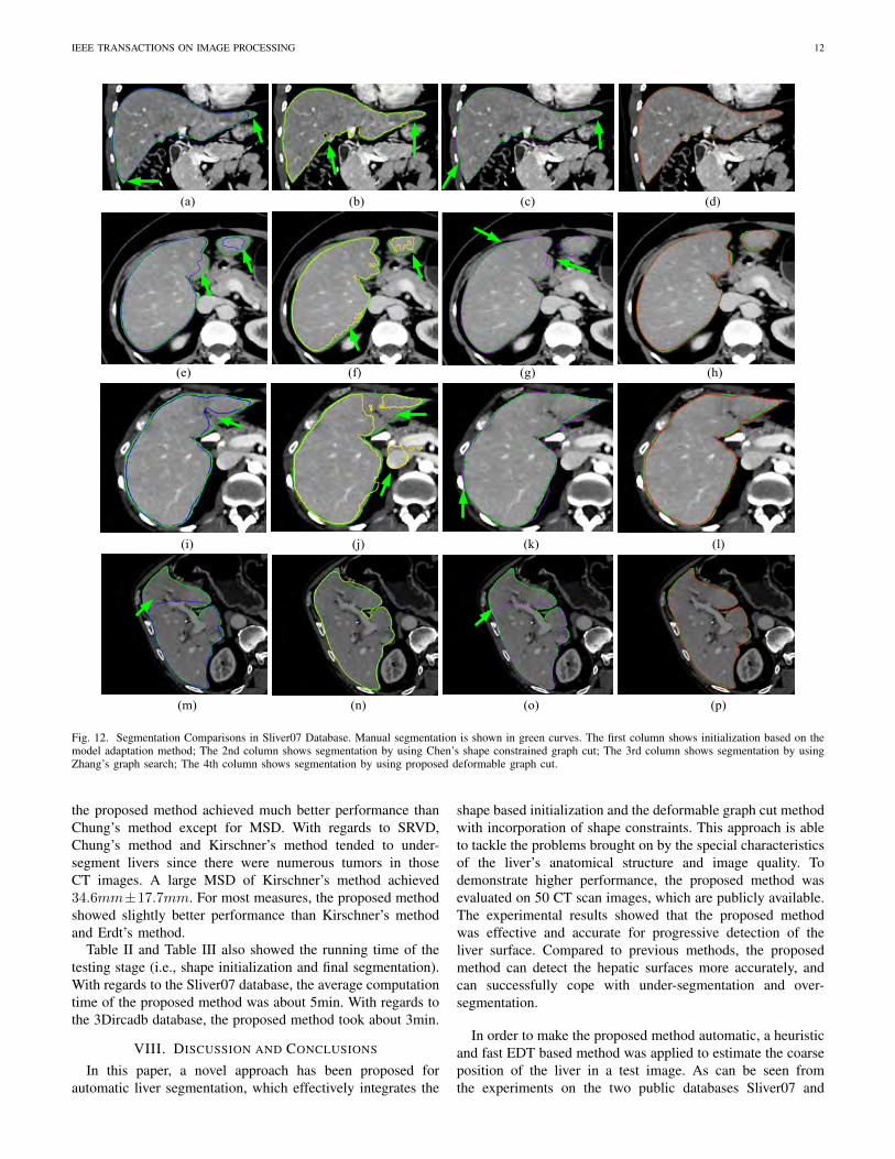
As can be seen in the 4th row, Chen’s method tended to ob-tain a under-segmented liver based on their shape constrainedgraph cut (the 2nd column of Fig.12), which integrated shapeprior into region term only. The maximal surface distanceof Zhang’s method is 24.8mm. Surface detection proposedby Zhang et. al. was applied along the normal direction

of surfaces, which also made it difficult to avoid under-segmentation and over-segmentation, as shown in the 3rdcolumn of Fig.12.

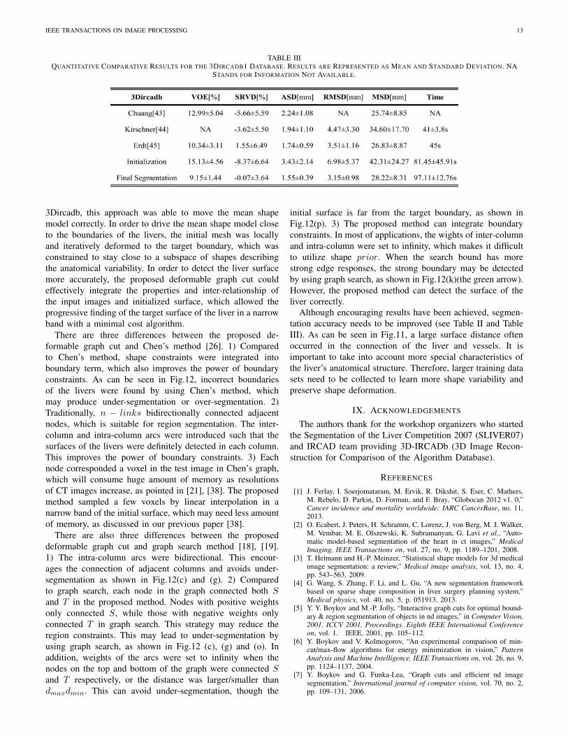
Table III shows the quantitative comparative results of theliver segmentation with previous methods in [44]–[46] and theproposed liver shape initialization and segmentation based onthe 3Dircadb database. For shape initialization results, modelinitialization was also far from accurate segmentation of theliver. Similarly, large distance to manual segmentation couldbe seen in the measures of ASD , RMSD and MSD, as canbe seen in the 4th row of Table III. For all of the datasets,


(a) (b) (c) (d)

(e) (f) (g) (h)

(i) (j) (k) (l)

(m) (n) (o) (p)

Fig. 12. Segmentation Comparisons in Sliver07 Database. Manual segmentation is shown in green curves. The first column shows initialization based on themodel adaptation method; The 2nd column shows segmentation by using Chen’s shape constrained graph cut; The 3rd column shows segmentation by usingZhang’s graph search; The 4th column shows segmentation by using proposed deformable graph cut.

the proposed method achieved much better performance thanChung’s method except for MSD. With regards to SRVD,Chung’s method and Kirschner’s method tended to under-segment livers since there were numerous tumors in thoseCT images. A large MSD of Kirschner’s method achieved34.6mm±17.7mm. For most measures, the proposed methodshowed slightly better performance than Kirschner’s methodand Erdt’s method.

Table II and Table III also showed the running time of thetesting stage (i.e., shape initialization and final segmentation).With regards to the Sliver07 database, the average computationtime of the proposed method was about 5min. With regards tothe 3Dircadb database, the proposed method took about 3min.

VIII. DISCUSSION AND CONCLUSIONS

In this paper, a novel approach has been proposed forautomatic liver segmentation, which effectively integrates the

shape based initialization and the deformable graph cut methodwith incorporation of shape constraints. This approach is ableto tackle the problems brought on by the special characteristicsof the liver’s anatomical structure and image quality. Todemonstrate higher performance, the proposed method wasevaluated on 50 CT scan images, which are publicly available.The experimental results showed that the proposed methodwas effective and accurate for progressive detection of theliver surface. Compared to previous methods, the proposedmethod can detect the hepatic surfaces more accurately, andcan successfully cope with under-segmentation and over-segmentation.

In order to make the proposed method automatic, a heuristicand fast EDT based method was applied to estimate the coarseposition of the liver in a test image. As can be seen fromthe experiments on the two public databases Sliver07 and


TABLE IIIQUANTITATIVE COMPARATIVE RESULTS FOR THE 3DIRCADB1 DATABASE. RESULTS ARE REPRESENTED AS MEAN AND STANDARD DEVIATION. NA

STANDS FOR INFORMATION NOT AVAILABLE.

3Dircadb, this approach was able to move the mean shapemodel correctly. In order to drive the mean shape model closeto the boundaries of the livers, the initial mesh was locallyand iteratively deformed to the target boundary, which wasconstrained to stay close to a subspace of shapes describingthe anatomical variability. In order to detect the liver surfacemore accurately, the proposed deformable graph cut couldeffectively integrate the properties and inter-relationship ofthe input images and initialized surface, which allowed theprogressive finding of the target surface of the liver in a narrowband with a minimal cost algorithm.

There are three differences between the proposed de-formable graph cut and Chen’s method [26]. 1) Comparedto Chen’s method, shape constraints were integrated intoboundary term, which also improves the power of boundaryconstraints. As can be seen in Fig.12, incorrect boundariesof the livers were found by using Chen’s method, whichmay produce under-segmentation or over-segmentation. 2)Traditionally, n − links bidirectionally connected adjacentnodes, which is suitable for region segmentation. The inter-column and intra-column arcs were introduced such that thesurfaces of the livers were definitely detected in each column.This improves the power of boundary constraints. 3) Eachnode corresponded a voxel in the test image in Chen’s graph,which will consume huge amount of memory as resolutionsof CT images increase, as pointed in [21], [38]. The proposedmethod sampled a few voxels by linear interpolation in anarrow band of the initial surface, which may need less amountof memory, as discussed in our previous paper [38].

There are also three differences between the proposeddeformable graph cut and graph search method [18], [19].1) The intra-column arcs were bidirectional. This encour-ages the connection of adjacent columns and avoids under-segmentation as shown in Fig.12(c) and (g). 2) Comparedto graph search, each node in the graph connected both Sand T in the proposed method. Nodes with positive weightsonly connected S, while those with negative weights onlyconnected T in graph search. This strategy may reduce theregion constraints. This may lead to under-segmentation byusing graph search, as shown in Fig.12 (c), (g) and (o). Inaddition, weights of the arcs were set to infinity when thenodes on the top and bottom of the graph were connected Sand T respectively, or the distance was larger/smaller thandmaxdmin. This can avoid under-segmentation, though the

initial surface is far from the target boundary, as shown inFig.12(p). 3) The proposed method can integrate boundaryconstraints. In most of applications, the wights of inter-columnand intra-column were set to infinity, which makes it difficultto utilize shape prior. When the search bound has morestrong edge responses, the strong boundary may be detectedby using graph search, as shown in Fig.12(k)(the green arrow).However, the proposed method can detect the surface of theliver correctly.

Although encouraging results have been achieved, segmen-tation accuracy needs to be improved (see Table II and TableIII). As can be seen in Fig.11, a large surface distance oftenoccurred in the connection of the liver and vessels. It isimportant to take into account more special characteristics ofthe liver’s anatomical structure. Therefore, larger training datasets need to be collected to learn more shape variability andpreserve shape deformation.

IX. ACKNOWLEDGEMENTS

The authors thank for the workshop organizers who startedthe Segmentation of the Liver Competition 2007 (SLIVER07)and IRCAD team providing 3D-IRCADb (3D Image Recon-struction for Comparison of the Algorithm Database).

REFERENCES

[1] J. Ferlay, I. Soerjomataram, M. Ervik, R. Dikshit, S. Eser, C. Mathers,M. Rebelo, D. Parkin, D. Forman, and F. Bray, “Globocan 2012 v1. 0,”Cancer incidence and mortality worldwide: IARC CancerBase, no. 11,2013.

[2] O. Ecabert, J. Peters, H. Schramm, C. Lorenz, J. von Berg, M. J. Walker,M. Vembar, M. E. Olszewski, K. Subramanyan, G. Lavi et al., “Auto-matic model-based segmentation of the heart in ct images,” MedicalImaging, IEEE Transactions on, vol. 27, no. 9, pp. 1189–1201, 2008.

[3] T. Heimann and H.-P. Meinzer, “Statistical shape models for 3d medicalimage segmentation: a review,” Medical image analysis, vol. 13, no. 4,pp. 543–563, 2009.

[4] G. Wang, S. Zhang, F. Li, and L. Gu, “A new segmentation frameworkbased on sparse shape composition in liver surgery planning system,”Medical physics, vol. 40, no. 5, p. 051913, 2013.

[5] Y. Y. Boykov and M.-P. Jolly, “Interactive graph cuts for optimal bound-ary & region segmentation of objects in nd images,” in Computer Vision,2001. ICCV 2001. Proceedings. Eighth IEEE International Conferenceon, vol. 1. IEEE, 2001, pp. 105–112.

[6] Y. Boykov and V. Kolmogorov, “An experimental comparison of min-cut/max-flow algorithms for energy minimization in vision,” PatternAnalysis and Machine Intelligence, IEEE Transactions on, vol. 26, no. 9,pp. 1124–1137, 2004.

[7] Y. Boykov and G. Funka-Lea, “Graph cuts and efficient nd imagesegmentation,” International journal of computer vision, vol. 70, no. 2,pp. 109–131, 2006.


[8] P. Campadelli, E. Casiraghi, and A. Esposito, “Liver segmentation fromcomputed tomography scans: A survey and a new algorithm,” ArtificialIntelligence in Medicine, vol. 45, no. 2, pp. 185–196, 2009.

[9] X. Zhou, T. Kitagawa, T. Hara, H. Fujita, X. Zhang, R. Yokoyama,H. Kondo, M. Kanematsu, and H. Hoshi, “Constructing a probabilisticmodel for automated liver region segmentation using non-contrast x-raytorso ct images,” in Medical Image Computing and Computer-AssistedIntervention–MICCAI 2006. Springer, 2006, pp. 856–863.

[10] E. van Rikxoort, Y. Arzhaeva, and B. van Ginneken, “Automaticsegmentation of the liver in computed tomography scans with voxelclassification and atlas matching,” in Proceedings of the MICCAI Work-shop 3-D Segmentation Clinic: A Grand Challenge. Citeseer, 2007,pp. 101–108.

[11] L. Rusko, G. Bekes, G. Nemeth, and M. Fidrich, “Fully automaticliver segmentation for contrast-enhanced ct images,” MICCAI Wshp. 3DSegmentation in the Clinic: A Grand Challenge, vol. 2, no. 7, 2007.

[12] A. H. Foruzan, R. A. Zoroofi, M. Hori, and Y. Sato, “Liver segmentationby intensity analysis and anatomical information in multi-slice ct im-ages,” International journal of computer assisted radiology and surgery,vol. 4, no. 3, pp. 287–297, 2009.

[13] R. Pohle and K. D. Toennies, “A new approach for model-based adaptiveregion growing in medical image analysis,” in Computer Analysis ofImages and Patterns. Springer, 2001, pp. 238–246.

[14] Y. Chen, Z. Wang, W. Zhao, and X. Yang, “Liver segmentation fromct images based on region growing method,” in Bioinformatics andBiomedical Engineering, 2009. ICBBE 2009. 3rd International Confer-ence on. IEEE, 2009, pp. 1–4.

[15] T. F. Cootes, A. Hill, C. J. Taylor, and J. Haslam, “The use of activeshape models for locating structures in medical images,” in InformationProcessing in Medical Imaging. Springer, 1993, pp. 33–47.

[16] H. Lamecker, T. Lange, and M. Seebass, Segmentation of the liver usinga 3D statistical shape model. Citeseer, 2004.

[17] D. Kainmuller, T. Lange, and H. Lamecker, “Shape constrained auto-matic segmentation of the liver based on a heuristic intensity model,”in Proc. MICCAI Workshop 3D Segmentation in the Clinic: A GrandChallenge, 2007, pp. 109–116.

[18] X. Zhang, J. Tian, K. Deng, Y. Wu, and X. Li, “Automatic liver segmen-tation using a statistical shape model with optimal surface detection,”IEEE Transactions on Biomedical Engineering, vol. 57, no. 10, p. 2622,2010.

[19] K. Li, X. Wu, D. Z. Chen, and M. Sonka, “Optimal surface segmentationin volumetric images-a graph-theoretic approach,” Pattern Analysis andMachine Intelligence, IEEE Transactions on, vol. 28, no. 1, pp. 119–134,2006.

[20] G. Wang, S. Zhang, H. Xie, D. N. Metaxas, and L. Gu, “A homotopy-based sparse representation for fast and accurate shape prior modelingin liver surgical planning,” Medical image analysis, vol. 19, no. 1, pp.176–186, 2015.

[21] H. Lombaert, Y. Sun, L. Grady, and C. Xu, “A multilevel banded graphcuts method for fast image segmentation,” in Computer Vision, 2005.ICCV 2005. Tenth IEEE International Conference on, vol. 1. IEEE,2005, pp. 259–265.

[22] N. Xu, N. Ahuja, and R. Bansal, “Object segmentation using graph cutsbased active contours,” Computer Vision and Image Understanding, vol.107, no. 3, pp. 210–224, 2007.

[23] L. Massoptier and S. Casciaro, “Fully automatic liver segmentationthrough graph-cut technique,” in Engineering in Medicine and BiologySociety, 2007. EMBS 2007. 29th Annual International Conference of theIEEE. IEEE, 2007, pp. 5243–5246.

[24] R. Beichel, A. Bornik, C. Bauer, and E. Sorantin, “Liver segmenta-tion in contrast enhanced ct data using graph cuts and interactive 3dsegmentation refinement methods,” Medical physics, vol. 39, no. 3, pp.1361–1373, 2012.

[25] M. G. Linguraru, W. J. Richbourg, J. Liu, J. M. Watt, V. Pamulapati,S. Wang, and R. M. Summers, “Tumor burden analysis on computedtomography by automated liver and tumor segmentation,” MedicalImaging, IEEE Transactions on, vol. 31, no. 10, pp. 1965–1976, 2012.

[26] X. Chen, J. K. Udupa, U. Bagci, Y. Zhuge, and J. Yao, “Medical imagesegmentation by combining graph cuts and oriented active appearancemodels,” Image Processing, IEEE Transactions on, vol. 21, no. 4, pp.2035–2046, 2012.

[27] H. Song, Q. Zhang, and S. Wang, “Liver segmentation based on skfcmand improved growcut for ct images,” in Bioinformatics and Biomedicine(BIBM), 2014 IEEE International Conference on. IEEE, 2014, pp. 331–334.

[28] S. Tomoshige, E. Oost, A. Shimizu, H. Watanabe, and S. Nawano, “Aconditional statistical shape model with integrated error estimation of the

conditions; application to liver segmentation in non-contrast ct images,”Medical image analysis, vol. 18, no. 1, pp. 130–143, 2014.

[29] X. Chen, M. Niemeijer, L. Zhang, K. Lee, M. D. Abramoff, and M. Son-ka, “Three-dimensional segmentation of fluid-associated abnormalitiesin retinal oct: probability constrained graph-search-graph-cut,” MedicalImaging, IEEE Transactions on, vol. 31, no. 8, pp. 1521–1531, 2012.

[30] F. Shi, X. Chen, H. Zhao, W. Zhu, D. Xiang, E. Gao, M. Sonka,and H. Chen, “Automated 3-d retinal layer segmentation of macularoptical coherence tomography images with serous pigment epithelialdetachments,” 2014.

[31] R. T. Whitaker and X. Xue, “Variable-conductance, level-set curvaturefor image denoising,” in Image Processing, 2001. Proceedings. 2001International Conference on, vol. 3. IEEE, 2001, pp. 142–145.

[32] W. E. Lorensen and H. E. Cline, “Marching cubes: A high resolution 3dsurface construction algorithm,” in ACM siggraph computer graphics,vol. 21, no. 4. ACM, 1987, pp. 163–169.

[33] H. Hoppe, “New quadric metric for simplifiying meshes with appear-ance attributes,” in Proceedings of the conference on Visualization’99:celebrating ten years. IEEE Computer Society Press, 1999, pp. 59–66.

[34] T. Heimann, I. Oguz, I. Wolf, M. Styner, and H.-P. Meinzer, “Imple-menting the automatic generation of 3d statistical shape models with itk,”in The Insight JournalłMICCAI Open Science Workshop, Copenhagen.Citeseer, 2006.

[35] B. K. Horn, “Closed-form solution of absolute orientation using unitquaternions,” JOSA A, vol. 4, no. 4, pp. 629–642, 1987.

[36] A. Meijster, J. B. T. M. Roerdink, and W. H. Hesselink, “A gen-eral algorithm for computing distance transforms in linear time,” inMathematical Morphology and its Applications to Image and SignalProcessing, Kluwer Acad. Publ., 2000, pp. 331–340.

[37] X. Chen, J. K. Udupa, A. Alavi, and D. A. Torigian, “Gc-asm: Synergis-tic integration of graph-cut and active shape model strategies for medicalimage segmentation,” Computer Vision And Image Understanding, vol.117, no. 5, pp. 513–524, 2013.

[38] D. Xiang, J. Tian, F. Yang, Q. Yang, X. Zhang, Q. Li, and X. Liu,“Skeleton cuts - an efficient segmentation method for volume rendering,”Visualization and Computer Graphics, IEEE Transactions on, vol. 17,no. 9, pp. 1295–1306, 2011.

[39] D. Zorin, P. Schroder, and W. Sweldens, “Interpolating subdivision formeshes with arbitrary topology,” in Proceedings of the 23rd annualconference on computer graphics and interactive techniques. ACM,1996, pp. 189–192.

[40] L. R. Herrmann, “Laplacian-isoparametric grid generation scheme,”Journal of the Engineering Mechanics Division, vol. 102, no. 5, pp.749–907, 1976.

[41] T. Heimann, B. Van Ginneken, M. A. Styner, Y. Arzhaeva, V. Aurich,C. Bauer, A. Beck, C. Becker, R. Beichel, G. Bekes et al., “Comparisonand evaluation of methods for liver segmentation from ct datasets,”Medical Imaging, IEEE Transactions on, vol. 28, no. 8, pp. 1251–1265,2009.

[42] A. Wimmer, G. Soza, and J. Hornegger, “A generic probabilistic activeshape model for organ segmentation,” in Medical Image Computing andComputer-Assisted Intervention–MICCAI 2009. Springer, 2009, pp. 26–33.

[43] M. G. Linguraru, W. J. Richbourg, J. M. Watt, V. Pamulapati, andR. M. Summers, “Liver and tumor segmentation and analysis from ct ofdiseased patients via a generic affine invariant shape parameterizationand graph cuts,” in Abdominal Imaging. Computational and ClinicalApplications. Springer, 2012, pp. 198–206.

[44] F. Chung and H. Delingette, “Regional appearance modeling basedon the clustering of intensity profiles,” Computer Vision and ImageUnderstanding, vol. 117, no. 6, pp. 705–717, 2013.

[45] M. Kirschner, “The probabilistic active shape model: From modelconstruction to flexible medical image segmentation,” Ph.D. dissertation,Citeseer, 2013.

[46] M. Erdt, S. Steger, M. Kirschner, and S. Wesarg, “Fast automaticliver segmentation combining learned shape priors with observed shapedeviation,” in Computer-Based Medical Systems (CBMS), 2010 IEEE23rd International Symposium on. IEEE, 2010, pp. 249–254.


Guodong Li received the B.E. degree in DalianUniversity of Technology, Dalian, China, in 2010.He is currently a Ph.D. candidate in the Key Lab-oratory of Molecular Imaging, Institute of Automa-tion, Chinese Academy of Sciences, Beijing, China.His current research interests include medical datasegmentation, medical image analysis, and patternrecognition.

Xinjian Chen received the Ph.D. degree from theCenter for Biometrics and Security Research, KeyLaboratory of Complex Systems and IntelligenceScience, Institute of Automation, Chinese Academyof Sciences, Beijing, China, in 2006. After com-pleting the graduation, he joined Microsoft ResearchAsia where he was involved in research on handwrit-ing recognition. From January 2008 to May 2012,he has conducted the Postdoctoral Research at sev-eral prestigious groups: Medical Image ProcessingGroup, University of Pennsylvania; Department of

Radiology and Image Sciences, National Institutes of Health; Departmentof Electrical and Computer Engineering, University of Iowa. On June 2012,he joined the School of Electrical and Information Engineering, SoochowUniversity, as a Full Professor. His research interests include medical imageprocessing and analysis, pattern recognition, machine learning, and their appli-cations. Up to now, he has published more than 70 high quality internationaljournal/conference papers. He is now a Distinguished Professor at SoochowUniversity, and serve as Director of a University level lab- Medical ImageProcessing, Analysis and Visualization Lab.

Fei Shi received the B.E. degree in Information andElectronics Engineering from Zhejiang University,Hangzhou, China, in 2002, and received the Ph.D. inElectrical Engineering from Polytechnic University, New York, USA, in 2006. Now she is an assistantprofessor at School of Electronics and InformationEngineering, Soochow University, Suzhou, China.Her current research interests include medical imageanalysis and pattern recognition.

Weifang Zhu received the B.E. and M.S. degreefrom Xi’an Jiaotong University, Shanxi, China, in2000 and 2003, respectively, and received the Ph.D.from Soochow University, Jiangsu, China, in 2013.Now she is an associate professor at School ofElectronics and Information Engineering, SoochowUniversity, China. Her current research interests in-clude medical image analysis, machine learning andpattern recognition.

Jie Tian (M’02−SM’06−F’10) received the Ph.D.degree (with honors) in artificial intelligence fromthe Institute of Automation, Chinese Academy ofSciences, Beijing, China, in 1992. From 1995 to1996, he was a Postdoctoral Fellow at the MedicalImage Processing Group, University of Pennsylvani-a, Philadelphia. Since 1997, he has been a Professorat the Institute of Automation, Chinese Academy ofSciences, where he has been the director of Key Lab-oratory of Molecular Imaging. His research interestsinclude the medical image process and analysis and

pattern recognition. Dr. Tian is an IEEE fellow, IAMBE fellow, SPIE fellow,AIMBE fellow.

Dehui Xiang received the B.E. degree in automationfrom Sichuan University, Sichuan, China, in 2007,and received the Ph.D. at the Institute of Automa-tion, Chinese Academy of Sciences, Beijing, China,in 2012. Now he is a associate professor at Schoolof Electronics and Information Engineering, Soo-chow University, Jiangsu 215006, China. His currentresearch interests include medical image analysis,computer vision, medical data visualization, andpattern recognition.

Documents

IEEE TRANSACTIONS ON IMAGE PROCESSING 1 Automatic Liver Segmentation ... · IEEE TRANSACTIONS ON IMAGE PROCESSING 1 Automatic Liver Segmentation based on Shape Constraints and Deformable