IEEE TRANSACTIONS ON ENERGY CONVERSION, VOL. 32, NO. 2

IEEE TRANSACTIONS ON ENERGY CONVERSION, VOL. 32, NO. 2, JUNE 2017 737

System-Level, FPGA-Based, Real-Time Simulationof Ship Power Systems

Matthew Milton, Andrea Benigni, Member, IEEE, and Jason Bakos, Member, IEEE

Abstract—In this paper, we present a scalable approach for real-time simulation of ship power systems with high-frequency powerelectronics converters (100–200 kHz). The proposed approach isbased on the latency-based linear multistep compound methodand relies on field-programmable gate array (FPGA) execution.Several examples of increasing dimension and complexity are usedto evaluate the scalability—both of in terms of computational de-lay and of resources usage—of the proposed approach. Real-timeexecution with a 50 ns time step is achieved for all the examplesconsidered.

Index Terms—Field-programmable gate arrays, parallel algo-rithms, power system simulation, power electronics, real timesystems.

I. INTRODUCTION

R EAL time simulation, Hardware In the Loop (HIL) andPower Hardware In the Loop (PHIL) techniques have been

widely used in the last twenty years to support design and anal-ysis of ship power systems. By filling the gap existing betweenfield test and traditional simulation, HIL and PHIL approachessignificantly de-risk the development of new designs. In [1] and[2], a high power PHIL set-up is used for the evaluation ofpropulsion motor and motor drives. A HIL set-up in [3] is alsoused for the testing of propulsion systems control. In [4], a HILset-up is used to evaluate a stabilizing control for MVDC shippower systems. Still in relation to MVDC ship systems, a highpower PHIL set-up is used in [5] to evaluate the impact of fastpower transfer between dynamic loads and in [6] to test faultmanagement approaches. In [7] and [8], simulation methods forexecution of real-time simulation with very small time step havebeen evaluated in the context of ship system simulation.

To be able to perform effective and accurate HIL and PHILtests, it is clear that real-time simulation execution at a propertime step is necessary. The selection of the time step dependson the dynamics of interest for the system simulated and for

Manuscript received June 24, 2016; revised December 22, 2016; acceptedApril 3, 2017. Date of publication April 7, 2017; date of current version May 18,2017. This work was supported in part by the Office of Naval Research (ONR)under Grant NOOO14-16-1-3042. Paper no. TEC-00542-2016. (Correspondingauthor: Andrea Benigni.)

M. Milton and A. Benigni are with the Department of Electrical Engineering,University of South Carolina, Columbia, SC 29208 USA (e-mail: [email protected]; [email protected]).

J. Bakos is with the Department of Computer Science and Engineering,University of South Carolina, Columbia, SC 29208 USA (e-mail: [email protected]).

Color versions of one or more of the figures in this paper are available onlineat http://ieeexplore.ieee.org.

Digital Object Identifier 10.1109/TEC.2017.2692525

the device under test. The needs of using a very small timestep and to simulate large systems have always been the mainchallenge of real time simulation. Over the last several decades,a significant amount of research and effort has been focusedon parallelizing electromagnetic transient stability simulations,mainly for real-time applications. Several approaches have beendeveloped based on latency effects (e.g., Bergeron line model)and on tearing approaches (e.g., Diakoptics). In the area of ter-restrial power systems, there has also been an increasing interest– specifically with the US Department of Energy – in the paral-lelization of transient stability simulation solvers. Historically,one of the main interests for real-time simulation in the electricalengineering field was the testing of relays for terrestrial powersystems [9], [10]. Starting in the same time, but with a significantgrowth of interest in recent years, real-time simulation and HILmethods for power electronic systems have attracted the interestof both academia and industry. The strong nonlinear behaviorof the systems and the small time step size required for the sim-ulation of power converters are the main challenges of real-timesimulation of power electronics systems. In the last few years,there has been an increasing use of new computational units toaddress these challenges: mixed solutions based on DSP/CPUand FPGA devices are increasingly common. FPGAs are usedboth as interface [11] and for computation: in [12]–[14] an ACmachine, a power converter and a nonlinear power transformerare directly simulated on an FPGA. In [15], a Modular Multi-level Converter (MMC) converter is simulated using an FPGAin combination with a CPU. In [16], a MMC is simulated in realtime using an FPGA with the goal of performing hardware-in-the-loop testing. In [17], the authors propose the use of an FPGAimplemented state space solver for the simulation of power elec-tronics converters. In [18], a multi-FPGA platform is used forthe simulation for the real-time electromagnetic transient sim-ulation of very large power systems. In [19], a test bench forthe HIL testing of electric vehicles is developed using FPGAbased real time simulation capability. In [20], a test bench forthe HIL testing of multiple-output power converters is realizedusing an FPGA platform. In [21], a tearing approach is proposedfor the parallel execution of the simulation of power electron-ics converter using and FPGA based platform. In [22], a mixedsolution based on CPU and FPGA is used to simulate a two-terminal MMC-HVDC system. In [23], the real time simulationof an MMC is executed on an FPGA platform including devicelevel details.In [24], an FPGA is used for the simulation of aninduction machine. In [25], the model of a permanent magnetmachines is executed on a FPGA platform for HIL testing.

0885-8969 © 2017 IEEE. Personal use is permitted, but republication/redistribution requires IEEE permission.See http://www.ieee.org/publications standards/publications/rights/index.html for more information.

738 IEEE TRANSACTIONS ON ENERGY CONVERSION, VOL. 32, NO. 2, JUNE 2017

Ship systems are expected to make large use of high switchingfrequency – 100-200 kHz – power electronic converters (e.g.,SiC based). Commercial tools, however, do not yet systemati-cally support scalable real-time simulation with very small timesteps – less than 100 ns – as required for simulation of highswitching frequency power electronics systems.

In [26], we developed and implemented a simulation methodthat we named Latency Based Linear Multi-step CompoundMethod (LB-LMC). The main idea of this method is to exploitthe small time step required for the simulation of high switchingfrequency converter to decouple the solutions of non-linear com-ponents from that of the rest of the system. In [26], we showedseveral examples executed in real time on DSP and CPU with atime step around 20µs.

In this paper, we introduce a modified version of the approachproposed in [26] to execute on FPGAs and take full advantage ofthe characteristic of these devices. Execution on FPGA devicesallows exploiting greater levels of parallelization than that onprevious platforms which create too much overhead in this re-gard. Moreover, FPGA execution eliminates any system latencytypical of CPU based systems and offers a very high scalability.Significant part of the paper is dedicated to explain how theLB-LMC method has been implemented and on the challengeassociated with it. The developed method is tested on ship sys-tem examples of different sizes to highlight the high scalabilityobtained.

II. LATENCY BASED LINEAR MULTI-STEP COMPOUND

METHOD

The Latency Based Linear Multi-step Compound Method(LB-LMC) is a highly parallelizable simulation method de-signed for real-time simulation of dynamic electrical systems. Inthis section, we provide a summary description of this methodwhich is detailed in [26].

The LB-LMC method is derived from the Resistive Compan-ion (RC) method, solving dynamic systems as a set of linearequations Gx = b every simulation time step, where G is theconductances of the system, b is the current contributions ofcomponents, and x is the node voltages of the system. In thispaper, we often use the term Resistive Companion to indicate ageneric method/solver similar to the ElectroMagnetic TransientsProgram (EMTP). Unlike traditional RC method, the LB-LMCmethod models all nonlinear components in a linear networksystem as functional voltage sources with series resistance, asseen in Fig. 1(a); or as current sources with parallel conduc-tance, as shown in Fig. 1(b). These series resistances or parallelconductances are held fixed and are inserted into the G con-ductance matrix to stay with standard form of RC components.The nonlinear behavior of the nonlinear components are thenreflected in the voltage or current source that is updated everysimulation step through an internal step that computes the stateequation of the component to update said source. The nonlinearcomponent state equations are expressed as:

dinidt

= f(v, i, xni , un

i , t) (1)

Fig. 1. Linear networks with nonlinear components. (a) With two nonlinearcomponents. (b) With one current-type nonlinear component.

dvnj

dt= f(v, i, xn

j , unj , t) (2)

where v is the vector of the network node voltages, i is thevector of the network branch currents, xn

i is the vector of thestate variable internal to the i-th nonlinear component, and ui

is the vector of the input internal to the i-th nonlinear compo-nent. Components with multiple terminals can be described bya mix of these current and voltage sources. These equations areexplicitly discretized to obtain:

Ini (k + 1) = f(v(k), i(k), xn

i (k), uni (k), k) (3)

V nj (k + 1) = f(v(k), i(k), xn

j (k), unj (k), k) (4)

Since the state equations for Ini and V n

j are explicitly discretizedand only depend on the solutions from previous time step, andthe equations are independent from one another, each nonlinearcomponent can perform its internal step in parallel to othercomponents. From these state equations, the source contributionvector b can be updated and the system solution each time stepcan be found with:

Gx(k + 1) = b(v(k), i(k), In (k), V n (k), k) (5)

From having the conductance matrix G held constant due toconsisting of only fixed conductances, LU factorization for theLB-LMC method system solver can be performed offline, andonly forward and backward substitution to solve the system isperformed each time step.

Fig. 2 shows the solution flow for LB-LMC. In this flow,G, x, and b are built from initial conditions and the LU fac-torization of the conductance matrix is performed. Once allnon-linear components are initialized, the simulation loop be-gins. Each iteration consists of each component performing itsown internal step in parallel, then the source vector b is updated.From the updated b vector, the system solution x is computedvia forward and backward substitution and saved for the nextstep. The simulation loop continues until final simulation time isreached.

The most important characteristic of the proposed approachis the use of explicit integration for the non-linear components,while the linear part of the network is integrated using an im-plicit numerical method. While the use of a Linear Multi-stepCompound method offers always better accuracy and stabilityproperty than the worst of the integration methods used, at the

MILTON et al.: SYSTEM-LEVEL, FPGA-BASED, REAL-TIME SIMULATION OF SHIP POWER SYSTEMS 739

Fig. 2. LB-LMC solution flow.

same time the use of an explicit integration algorithm always im-plies some concern related to stability and accuracy. In [26] —where we first presented the method — we performed a completestability analysis of the proposed method. We showed severalexamples related to power electronics systems and multi-physicapplications and most important we showed how for powerelectronics system the selection of the time step is driven by theswitching frequency of the converters and not by the stabilityand accuracy limit of the proposed LB-LMC approach.

III. FPGA ENCAPSULATION

In this section, the encapsulation of the LB-LMC methodelements for FPGA implementation is explained.

A. Component Entities

For each nonlinear component type used to model a system,a FPGA entity is developed. As input, these component entitiestake the system solution computed in a previous time step. Alongwith system solution, component entities can also take otherinput signals to control behavior of the entity, such as switchcontroller signals for a DC/AC converter component. At thebeginning of each time step, the component entities sample andregister their inputs. From these inputs and past internal states,the components perform their internal step for (3) and/or (4) andcompute their source contributions.

The component entities perform computational operationsfor their internal step in a non-pipelined, dataflow (data-driven)manner. In this manner, all internal step operations are imme-diately executed in response to any changes in the componententity inputs, or in the results passed between operations. More-over, these operations are all performed in parallel to one an-other, no matter the dependency between operations. Due tothis execution flow, internal step operations never wait on pre-requisite operations to finish to begin their own execution, theoperations converging to correct results as prerequisite onescomplete. All internal step operations of a component are ex-pected to complete with correct results within a single passbefore new inputs are registered.

An example component entity for a DC/AC converter (seeFig. 8) is depicted in Fig. 3. The DC/AC converter entity takesfive inputs that are the DC bus and AC phase voltages on

Fig. 3. Example of DC/AC converter component entities.

the terminals of the converter, and three switch control inputsto control the output phase modulation. Each time step, thecomponent will register its past states and inputs from step kthen use these to execute its internal step. The internal step forthe converter involves handling the switching action of the con-verter through toggling bus capacitor voltages and filter induc-tor currents (a, b, c, ac1 , bc1 , cc1 , etc.) and computing the saidcapacitor and inductors states for the current time step k + 1.The source contribution computational step (dashed block) com-putes the source currents for the bus capacitors and feeds thesecurrents and the inductor currents out as the contribution output.Using dataflow execution in the DC/AC converter entity, all ofthe internal step operations, as depicted in Fig. 3, are executedin parallel, propagating results to dependent operations withoutwait until the source contributions of the component convergeto correct results in a single pass.

B. System Solver Entity

A dedicated system solver FPGA entity is created to computethe system solution. This solver entity takes as input the compo-nent source contributions and accumulates these contributionstogether to create the whole source vector b used to compute thesystem solution. The entity provides the system solution vectorx as output which are fed back to component entities as inputfor the next time step execution.

Unlike the original LB-LMC method, the system solverentity does not use forward-backward substitution for system so-lution computation. Instead, this entity uses an inverted conduc-tance matrix precomputed offline and multiple algebraic sum ofproduct (SOP) expressions to find the system solution. In thisapproach, the system solution is found by solving (5) for thevector x like in (6), where A is the inverted G conductancematrix (A = G−1).

b = f(v(k), i(k), In (k), V n (k), k)

x(k + 1) = Ab (6)

This solution is computed by expanding the multiplicationbetween A and b matrices into SOP expressions, like seen in (7),which are to be each computed individually from one another.Since the inverted conductance matrix is fixed, the A terms in the


Fig. 4. Separation of subsystems.

SOP expressions can be defined as constants in said expressions.

x = Ab ⇒

A11b1 + A12b2 + · · · + A1nbn

A21b1 + A22b2 + · · · + A2nbn

...

An1b1 + An2b2 + · · · + Annbn

(7)

One main benefit of using this approach over forward-backwardsubstitution is division operations are not required in calcula-tions which tend to be computationally more expensive time-wise and use more FPGA resources compared to addition andmultiplication operations. Moreover, this approach has onlySOP expressions for the system that can be solved for sys-tem solution elements in parallel. A disadvantage to using thisapproach is that since the A matrix is precomputed offline andthe SOP expressions are dependent solely on the system beingmodeled, the system solver entity and its expressions will haveto be recreated or modified for each new system that is to besimulated.

IV. SYSTEM SOLVER REALIZATION

In this section, we detail how the system solver can be de-signed to realize desired FPGA resource usage and computa-tional latency.

A. Subsystem Decomposition

Due to how the nonlinear behavior of components is movedto the source contribution computations from the conductancematrix in LB-LMC, it is possible to have multi-terminal com-ponents modeled as separate elements whose conductances areindependent from one another. Then, the elements’ behavior iscoupled together via the component’s internal step to properlymodel the whole component. For example, if we consider thethree phase DC/AC converter discussed in Section III, from asystem solver point of view the converter reduces to a set ofvoltage and current sources, as seen in Fig. 5. A component likethis may lead to a global conductance matrix that is block diag-onal with up to six different blocks, even if this is not typicallythe case because other components may create links betweenthe different subsystems; at the least, fewer diagonal blocks areobtained. It is important to underline that in any case the user is

Fig. 5. DC/AC converter system solver structure.

never involved in this process. To help the reader understand thepracticality of this approach in real system models, we indicatein Section VIII how many subsystems are obtained for each ofthe models considered. From exploiting this possible separationof elements, the overall system model is expressed to containindependent subsystems which appear as independent diagonalblocks on the conductance matrix. A subsystem solver can becreated from each diagonal block matrix and operated sepa-rately to compute a sub-vector of the solution. These subsystemsolvers can be encapsulated into the top level system solver. Theimpact of using subsystem solvers is that the number of termsper system solution equation can be reduced substantially, low-ering amount of FPGA hardware resources required.

An example of this subsystem separation for a 12-node systemis shown in Fig. 4. In this example, the system has two 4-nodesubsystem blocks and four 1-node blocks. If this system wassolved without subsystem decomposition, 144 multiplicationsand 132 additions would be needed. However, with the decom-position, the operations are reduced to 36 multiplication and 24additions, significantly reducing resources needed for the sys-tem solver. The shipboard power system models we present inthis paper are expressed with a similar structure as this example.

B. System Solver Architecture

The system solver is implementable using two types of ar-chitecture: dataflow execution that solves solution equationsin parallel, data-driven manner within one pass, and multi-cycleexecution which solves solution equations sequentially in multi-ple iterations within single time step. These architecture designsare explained below.

1) Dataflow Execution: In the dataflow implementation, thesystem solver solves all of its SOP solution equations entirely inparallel using a data-driven approach. All solution equationsare each given dedicated computational units, composed ofcombinational multiplier and adder units on the host FPGA,which operate independently from each other. As componentsource contributions are provided to the system solver, the com-putational units will compute the system solutions immedi-ately without the need to wait on any control or clock signalto initiate the computations; only the input contributions are


Fig. 6. Simulation engine.

required to start computation. This approach allows solutions tobe produced without delays induced from performing clockedoperations sequentially.

2) Multiple Cycle Execution: Another approach to imple-menting the system solver is to have it compute the systemsolution within multiple clock cycles per time step. In this ap-proach, the solution equations are broken up into like operations.These like operations are then executed sequentially, with a setnumber of operations executed per clock cycle. After all opera-tions of the solution equations are executed over multiple clockcycles, the results of each operation are compiled or accumu-lated to reach the complete system solution. The equation oper-ations are performed by computational units which are reusedevery clock cycle as the operations are expected to be identicalbut with different inputs. The reuse of the same computationalunits every iteration allows reduction of FPGA resource usagefor larger system models though at the expense of additionalcomputational latency per time step from executing operationssequentially.

An effective usage of multi-cycle execution is to iterate thesolving of each subsystem block in a model. With such a setup,each subsystem block is solved each cycle of the system solver.If a model has sizable but few subsystem blocks, then usingsame subsystem solver and iterating it per subsystem can no-ticeably reduce resource usage while maintaining low enoughclock latency for nanosecond-range time steps.

V. SIMULATION ENGINE COMPOSITION

This section provides explanation of how the entity encapsu-lations of the components and system solver are linked togetheron FPGA hardware to perform simulations.

To perform simulation of a system with the FPGA-adaptedLB-LMC method, a simulation engine like seen in Fig. 6 iscomposed, consisting of multiple component entities and onesystem solver entity tailored to the system simulated. In theengine, a component entity for each nonlinear component of thesystem is instanced and their source contribution outputs are

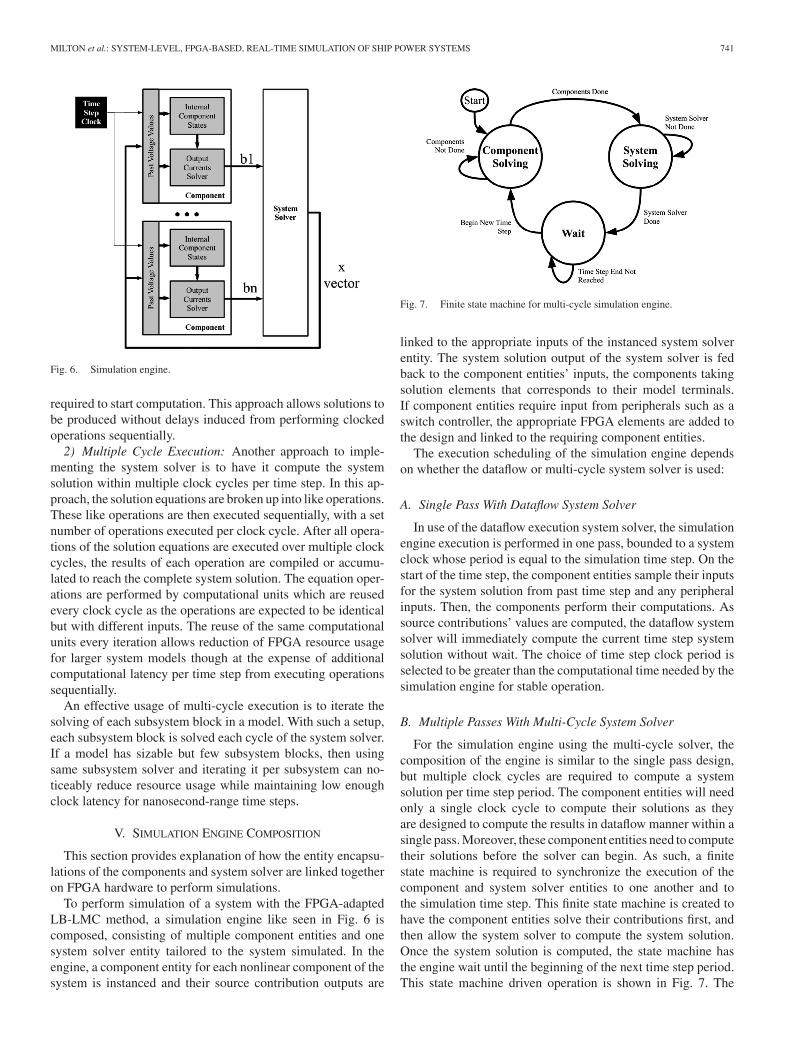
Fig. 7. Finite state machine for multi-cycle simulation engine.

linked to the appropriate inputs of the instanced system solverentity. The system solution output of the system solver is fedback to the component entities’ inputs, the components takingsolution elements that corresponds to their model terminals.If component entities require input from peripherals such as aswitch controller, the appropriate FPGA elements are added tothe design and linked to the requiring component entities.

The execution scheduling of the simulation engine dependson whether the dataflow or multi-cycle system solver is used:

A. Single Pass With Dataflow System Solver

In use of the dataflow execution system solver, the simulationengine execution is performed in one pass, bounded to a systemclock whose period is equal to the simulation time step. On thestart of the time step, the component entities sample their inputsfor the system solution from past time step and any peripheralinputs. Then, the components perform their computations. Assource contributions’ values are computed, the dataflow systemsolver will immediately compute the current time step systemsolution without wait. The choice of time step clock period isselected to be greater than the computational time needed by thesimulation engine for stable operation.

B. Multiple Passes With Multi-Cycle System Solver

For the simulation engine using the multi-cycle solver, thecomposition of the engine is similar to the single pass design,but multiple clock cycles are required to compute a systemsolution per time step period. The component entities will needonly a single clock cycle to compute their solutions as theyare designed to compute the results in dataflow manner within asingle pass. Moreover, these component entities need to computetheir solutions before the solver can begin. As such, a finitestate machine is required to synchronize the execution of thecomponent and system solver entities to one another and tothe simulation time step. This finite state machine is created tohave the component entities solve their contributions first, andthen allow the system solver to compute the system solution.Once the system solution is computed, the state machine hasthe engine wait until the beginning of the next time step period.This state machine driven operation is shown in Fig. 7. The


bounding of the entities’ solution computation to each enginestate is done through use of start input signals of each entitywhich is triggered by the state machine during each state.

VI. FPGA IMPLEMENTATION

We discuss in this section the implementation of the LB-LMC simulation engines in regard to how computation execu-tion is scheduled for parallelism and how numerical quantitiesare stored and processed.

For high scalability of performance of the LB-LMC methodon FPGAs, the parallelism of FPGA hardware is exploited to ac-celerate computations. To utilize this high parallelism, all equa-tion computations in component entities are expressed to beexecuted independently where possible, allocated to dedicatedarithmetic units for each equation so that they can be solved inparallel. Furthermore, to avoid serial data paths in componententity computations, solution equations are expressed to avoiddependencies between one another where allowed by the com-ponent’s model and solution integration method. Furthermore,all component entities are instanced with independent hardware.

Parallelism is also exploited in the system solver. For thedataflow solver, all system solution equations like seen in (7)are expressed to have dedicated arithmetic hardware providedto each one so they can be scheduled to run simultaneously.Moreover, the equations are implemented in dataflow manner,as discussed before, in the form of pure combinational logiccomposed of Lookup Table (LUT) and DSP slices which com-pute new solutions as soon as source contribution results change.This execution manner allows solutions to be computed as soonas possible without having to wait for all source contributions tobe computed by the component entities. In the multi-cycle sys-tem solver, the solution equations, though terms are looped, arealso all implemented with separate hardware as well. Due to therepeated use of the arithmetic hardware in the multi-cycle solverfor each solution equation during each time step, this hardwareis pipelined to reduce number of cycles needed to reach a solu-tion to be equal to number of terms per equation plus any cyclesneeded to fill the pipelines.

So that computational delays for the component entities andsystem solver is reduced and mostly dependent on the lowpropagation delays of the FPGA primitives, fixed-point arith-metic logic is used instead of floating-point logic for all cal-culations performed within. Common floating-point arithmeticimplementations, such as IEEE 754, typically require complex,high-latency, pipelined operations to handle their sophisticatedformats. Fixed-point arithmetic logic, on the other hand, can beeasily created with simpler combinational logic for integer arith-metic which does not require pipelining. Due to not needing tobe clocked or pipelined to produce an output, fixed-point com-putational delay can depend almost solely on propagation delayof the comprised logic primitives. Since fixed point arithmetichardware is much simpler than floating point hardware, thesepropagation delays can be kept low. Moreover, many FPGAplatforms have built-in integer DSP slices or blocks which canbe applied to accelerate operations and reduce delays of in-teger and fixed-point arithmetic. The main downside to using

fixed-point arithmetic is limited numerical precision comparedto floating point, which can adversely affect numerical stabilityand accuracy. However, this limitation can be alleviated withcareful selection of integral and fractional bit widths for fixedpoint signals within a simulation, giving numerical accuracycomparable to use of floating point arithmetic.

VII. SCALABILITY

This section discusses the scalability of the FPGA implemen-tation of the LB-LMC solver as model size increases, in terms ofachievable time step (computation delay), clock cycle latency,and FPGA resource usage.

A. Components

The number of operations required to compute the internalstates and source contributions of a component is largely de-pendent on the component model and integration method used.However, the total number of operations required for a collec-tion of components of same model and type will scale linearly asmore components of same type are instanced in a simulation en-gine. This linear scaling of operations also applies to resourceusage as each operation of same type uses similar amount ofresources. Though resource usage will increase linearly withnumber of components, the computational delay for all compo-nents of same type to perform their operations will stay constantdue to the parallel operation of said components.

B. Dataflow System Solver

As the size of a modeled, independent system or subsystemgrows to n solutions, the number of operations required for thesolver grows by an order of 2, with number of multiplicationsneeded being n2 , and additions being n(n − 1). If each opera-tion type (multiplication or addition) is mapped to unchangingFPGA resources without any FPGA synthesis optimizations,the amount of resources needed for the dataflow will also growby an order of 2 as well. Due to this growth of resources, thesystem solver can act as a bottleneck that determines how largeof a model and its simulation engine can fit on a given FPGAdevice. To reduce number of operations and FPGA resourcesin the dataflow system solver, the modeled system is broken upinto subsystems where possible and each subsystem is given itsown solver with reduced size n.

The computation delay of the dataflow system solver willgrow sublinearly as a model size increases due to the multipli-cation and addition operations performed in parallel, dataflowmanner on FPGA hardware. This scaling is unlike a traditionalCPU or DSP whose computational time or delay for the solvingof these system equations will grow with an order of 2 as thenumber of solutions increases, due to performing all operationssequentially.

C. Multi-Cycle System Solver

The number of operations implemented in hardware of themulti-cycle system solver is inversely proportional to the num-ber of iterations selected for the solver to compute a solution.


Resource usage will scale similarly, though extra resources arerequired to enable multi-iteration computation and pipelining.Computational time of the system solver is a function of cyclesneeded for the solver to reach solution, where the time is a prod-uct of the number of cycles, including extra cycles for pipelinepriming, and the clock period used.

D. Simulation Engine Time Step and Computation Delay

The time step usable for the simulation engine is dependenton the computational delay and latency of the components andsystem solver. With the dataflow system solver, the time stepmust be greater than the sum of computational delay requiredfor the slowest component entity type and the delay needed forthe system solver to have all solutions computed and stabilized;this sum being the total computational delay of the simulationengine:

Δt > tsolver + tcomp delay (8)

For larger system models, it is expected that the simulationengine computational delay will be dominated by the systemsolver delay as component model entities’ delays do not growwith system size and expected to typically be small in compu-tational complexity. To greatly reduce system solver delay, andreduce time step, subsystem decomposition can be used withinthe system solver as noted before.

In the case of using a multi-cycle system solver, the systemsolver will again greatly influence the time step for the simu-lation engine due the solver’s need for multiple cycle latencyneeded to reach the system solution each time step. The compu-tation time of the simulation engine will be the number of cyclesneeded for system solver to reach solution times the clock periodused to clock the solver, plus the delay needed for the slowesttype of component entities to perform their operations. Fromthis relation, the time step will have to be:

Δt > nsol cyclestclk + tcomp delay (9)

Reduction of multi-cycle system solver latency, and in turn thetime step, can be achieved through reducing the number ofcycles needed to compute the solution through performing moresystem solution equation operations per cycle, or to an lessereffect, reduce the clock period. In either case, the tradeoff ishigher usage of FPGA resources.

VIII. TEST MODELS

In this section, the power electronic system models used toevaluate the LB-LMC FPGA simulation engine is discussed.Each model is of increasing size and complexity.

A. Three-Phase DC/AC Converter

A three-phase DC/AC converter, depicted in Fig. 8, is mod-eled in LB-LMC method using parameters seen in Table I. Theconverter operates with 12 kV DC input. Switching frequencyfor the converter is 100kHz. The switching devices are mod-eled using a switching function approach similarly to what isdescribed in [27]. The component entity of the converter model

Fig. 8. Three phase DC/AC converter.

TABLE IDC/AC CONVERTER MODEL PARAMETERS

VD C CD C B u s LF i l t e r CF i l t e r RL o a d

12000 0.001 0.0001 1.0e-6 7.0

Fig. 9. Single bus shipboard power system.

separates its internal elements into independent subsystems toallow subdividing the system solver into smaller block solvers,though the elements are coupled analytically through the inter-nal step equations. Overall system has five node voltage solu-tions to solve, each associated with a 1-node subsystem block.During the Component Solving state in Fig. 7, the internal equa-tions of the three phase DC/AC converter are updated togetherwith the voltage and current across and through the other dy-namic components of the circuit. In the System Solving state,the node voltages are obtained using the approach described inSection III-B and using the equivalent circuit of Fig. 5 for theAC/DC converter.

B. Single Bus Shipboard Power System

A single-bus power system found on ships, shown in Fig. 9,is modeled using same converter model and parameters as thethree-phase converter system, with other parameters chosen tohave total system operate with 40 MW load. This system con-tains three converters and uses a straight DC input source of12 kV. The overall system has 23 node voltage solutions tosolve, and consists of two 7-node subsystem and nine 1-nodesubsystem blocks.

C. Dual Bus Shipboard Power System

A dual-bus shipboard power system, displayed in Fig. 10, issimilar to the single-bus system, but is composed of six DC/ACconverters and two DC/DC converters. Parameters for this sys-tem is set for 40MW load and the DC/DC converters are set tooutput 12kV DC voltage onto bus lines. The overall system has


Fig. 10. Dual bus shipboard power system.

Fig. 11. Top level design for simulation platform.

54 nodes, and consists of two 16-node subsystem and twenty-two 1-node subsystem blocks. Similar to what was indicated forthe DC/AC converter case, the power converter internal equa-tions and current/voltage across/through operations are updatedin the Component Solving state depicted in Fig. 7.

IX. IMPLEMENTATION RESULTS

In this section, we reveal results taken from separate LB-LMC FPGA simulation engines modeling in real-time the threepower electronic systems discussed in Section VIII. All modelswere run at 50 ns time step, using the dataflow system solver.Resource usage and clock cycle latency of the dual-bus powersystem simulation engine using the multi-cycle system solver isalso presented.

A. Setup

For all three models, the same top-level FPGA design wasused, shown in Fig. 11. The simulation engine was developedin C++ under Xilinx Vivado HLS 2015.4, and the complete top-level design was composed in standard Vivado using VHDL forthe Xilinx Virtex-7 VC707 FPGA evaluation board. The FPGAwas provided a 200 MHz (5 ns) clock source to serve as pri-mary clock for all internal logic. This clock source was divideddown to a 50 ns clock within the top-level design to drive thesimulation engine. All numerical operations in the simulationengine were performed with fixed point logic defined with HLSap_fixed library, using 72-bit width with 43-bit fractional pre-cision. The engine controller seen in Fig. 11 handles the startand reset of the simulation engine, as well as the wait stateof the simulation engine’s finite state machine when using amulti-cycle system solver. All models were run with open-loopswitching control to minimize impact of correcting control ac-tion on simulation results.

TABLE IIMODEL ERROR

Three-PhaseInverter

Single-BusShipboard System

Dual-Bus ShipboardSystem

C++ LB-LMC (%) 85.97e-06 0.0087 0.0141Traditional RC (%) 1.0034 0.6545 0.5221

Fig. 12. Error comparison for three phase inverter.

B. Simulation Accuracy and Error

To validate the accuracy of the results for each model, allsystem solution results, logged from the RTL-simulation of eachmodel simulation engine design, is compared for error to apure C++ implementation of the LB-LMC solver running atsame time step length, using double precision floating pointdata type. Moreover, error comparison is made to a traditionalresistive companion-based simulator running with 500 ps timestep. The error, shown in Table II was computed using two-norm(Euclidean) error equation, expressed here:

error% =‖x̂ − x‖2

‖x‖2100% (10)

where x̂ is a matrix of all solutions taken over a 50 ms simula-tion time period from the simulation engine and x is the matrixof all solutions from the reference solver in same time frame.As can be seen from the table, going to fixed point from doublefloating point data type has minimal impact on the the accuracyof the solver implementation, with error around 0.1 percent andbelow. Compared to the traditional RC solver (EMTP), someaccuracy is lost from applying LB-LMC solver. However, accu-racy between solvers is still reasonably similar, with percentagesof around one percent and less. To better appreciate the impactof the LB-LMC solver on simulation accuracy, we compare theresults obtained using the LB-LMC with the one obtained usinga traditional RC solver (EMTP) in Fig. 12. For this compari-son, we used the DC bus and phase A voltages on the secondconverter of the single bus shipboard power system example.

C. Scalability

The FPGA resource usage and per-time-step computationdelay of the simulation engine of each test model was cap-tured from reports given after full implementation from Vivado,


TABLE IIIRESOURCE USAGE AND COMPUTE DELAYS

Three-PhaseInverter

Single-BusShipboard System

Dual-Bus ShipboardSystem

Time Step (ns) 50.0 50.0 50.0Compute Delay (ns) 42.8 48.3 48.7DSP 170 (6.1%) 712 (25%) 1884 (67%)LUT 3943 (1.3%) 32558 (11%) 87525 (29%)FF 893 (0.1%) 3637 (0.6%) 8932 (1.5%)

Fig. 13. Single-bus power system analog output.

results shown in Table III, with percentage of Virtex-7 FGPAresources used in parentheses. Results from the engine onlyare shown, not of the complete top-level design with peripheralhardware. As can be seen from the results, the computationaldelays stayed low enough to allow the small time step to be usedfor each model in real-time, despite large growth in model size.Total resource usage scaled approximately linearly. Much of theresource usage increase between models is from the increasein number of component entities whose resources scale almostlinearly with amount of components of each type. Applying thesubsystem decomposition for the system solver allows the re-source usage there to increase more linearly in the case of thesemodels, compared to increasing by an order of two withoutsubsystem break-up.

D. Real-Time Performance

The FPGA implementation is capable of simulating the pre-sented power systems with a time step of 50 ns in real-time asseen in Table III.

E. Demonstration

The simulation engine designs of the two shipboard systemsare loaded onto the VC707 FGPA board and analog output ofeach model was captured, via an oscilloscope, from their respec-tive engine; results seen in Figs. 13 and 15. For the single-bussystem model results, three AC output phases from one of theDC/AC converters is shown. The dual-bus system results dis-play two of the output phases and the positive and negative DCbus line voltages. The results for the single-bus system werecaptured while switch control for the DC/AC converters wasset to reduce phase output voltage by half suddenly. In Fig. 14,we report a zoom of the associated transient. Similarly, the

Fig. 14. Single-bus power system analog output, phase 1 zoom.

Fig. 15. Dual-bus power system analog output.

dual-bus system results were captured while the switch controlof the DC/DC converters powering the system was set to re-duce bus voltage to simulate sudden drop in DC/DC convertervoltages. Ringing in the dual-bus system voltages is consistentwith traditional RC version of said system, and is expecteddue to operating without closed-loop control to correct for theoscillations.

F. Multi-Cycle System Solver Resource Usage

To evaluate impact on resource usage from using a multi-cycle system solver with subsystem iteration, the system solverfor the dual-bus shipboard system was implemented in Vivadowith the dataflow design and the multi-cycle design for a 50 nsclock cycle, where the dataflow is expected to compute its solu-tion before 50 ns while the multi-cycle design is clocked every50 ns. Each version of the solver was implemented separatefrom the top-level design so that the resource usage reportsshown the system solvers’ usage only. The multi-cycle versionwas designed to use same subsystem solver unit for the two sub-systems in the shipboard system and compute all solutions andbe prepared to receive new source contribution inputs withintwo cycles; effectively doubling the feasible time step. Bothversions solved the 1-node subsystems all in parallel to the sub-system computations. The resource usage of the two systemsolver architectures and their usage percentage on the Virtex-7FPGA is shown in Table IV. As can be seen from the results,using the multi-cycle design reduced DSP and LUT usage ofthe total system solver by approximately 33-36% compared tothe dataflow design while still allowing the simulation engine


TABLE IVRESOURCE USAGE FOR MULTI-CYCLE SYSTEM SOLVER

Dataflow Multi-Cycle

Cycles 0 2DSP 724 (26%) 466 (17%)LUT 54172 (18%) 36349 (12%)FF 0 (0%) 3830 (0.6%)

to perform with a reasonable 100 ns time step. Though not anone-to-one tradeoff between latency and resource usage, thisresource reduction is significant enough to highlight that thismulti-cycle approach can enable simulation engines of largemodels to potentially fit on a given FPGA where resource us-age of a dataflow solver may not allow. Flip-flop usage wentup from needing to maintain memory for the iterations of themulti-cycle architecture, but usage percentage on the Virtex-7is insignificant at below one percent.

X. CONCLUSION

This paper presents the FPGA implementation of the LB-LMC method for scalable, real-time simulation of ship powersystems. Using the parallelism and low-latency of FPGA de-vices, the adapted LB-LMC method is able to simulate powersystems of dramatically increasing size while still maintainingeffective scaling of computational delays to realize constant timestep of 50 ns. Despite maintaining scalable time steps, FPGAresource usage is still a concern for larger system models whichcan be compensated for through use of subsystem decomposi-tion allowed by the LB-LMC method. As is seen in the results,the use of a multi-cycle solver can also reduce hardware usageat cost of increased computational time and time step, thoughchallenges exist to implement the multi-cycle architecture tohave one-to-one or better trade-off between resource usage andcomputational time. While the LB-LMC FPGA implementationperforms well, modeling accuracy is not sacrificed as simulationresults deviated little from that of traditional resistive companionmethod solvers.

REFERENCES

[1] M. Steurer et al., “Hardware-in-the-loop investigation of rotor heating ina 5 MW HTS propulsion motor,” IEEE Trans. Appl. Supercond., vol. 17,no. 2, pp. 1595–1598, Feb. 2007.

[2] M. Steurer, C. S. Edrington, M. Sloderbeck, W. Ren, and J. Langston,“A megawatt-scale power hardware-in-the-loop simulation setup for mo-tor drives,” IEEE Trans. Ind. Electron., vol. 57, no. 4, pp. 1254–1260,Apr. 2010.

[3] Z. Lin, H. Chen, H. Gao, and K. Zhan, “Hardware-in-the-loop simulationof marine electric propulsion system,” in Proc. IEEE Elect. Ship Technol.Symp., 2015, pp. 104–108.

[4] M. Cupelli, M. de Paz Carro, and A. Monti, “Hardware in the loop imple-mentation of linearizing state feedback on MVDC ship systems and thesignificance of longitudinal parameters,” in Proc. Int. Conf. Elect. Syst.Aircr., Railw., Ship Propulsion Road Vehicles, 2015, pp. 1–5.

[5] M. Bosworth, D. Soto, M. Sloderbeck, J. Hauer, and M. Steurer, “MW-scale power hardware-in-the-loop experiments of rapid power transfersin MVDC naval shipboard power systems,” in Proc. IEEE Elect. ShipTechnol. Symp., 2015, pp. 459–463.

[6] M. Andrus, H. Ravindra, J. Hauer, M. Steurer, M. Bosworth, and R.Soman, “PHIL implementation of a MVDC fault management test bed forship power systems based on megawatt-scale modular multilevel convert-ers,” in Proc. IEEE Elect. Ship Technol. Symp., 2015, pp. 337–342.

[7] R. Crosbie, J. Zenor, D. Word, R. Bednar, and N. G. Hingorani, “A low-cost high-speed real-time simulator for ships power systems,” in Proc.IEEE Elect. Ship Technol. Symp., 2011, pp. 102–105.

[8] R. Crosbie, J. Zenor, D. Word, R. Bednar, and N. G. Hingorani, “Advancesin high-speed real-time multi-rate simulation techniques for ship powersystems,” in Proc. IEEE Elect. Ship Technol. Symp., 2009, pp. 165–169.

[9] P. McLaren, R. Kuffel, R. Wierckx, J. Giesbrecht, and L. Arendt, “A realtime digital simulator for testing relays,” IEEE Trans. Power Del., vol. 7,no. 1, pp. 207–213, Jan. 1992.

[10] R. Kuffel, J. Giesbrecht, T. Maguire, R. P. Wierckx, and P. McLaren ,“Advances in high-speed real-time multi-rate simulation techniques forship power systems,” in Proc. Int. Conf. Digit. Power Syst. Simulators,1995, pp. 19–24.

[11] H. Figueroa, A. Monti, and X. Wu, “An interface for switching signalsand a new real-time testing platform for accurate hardware-in-the-loopsimulation,” in Proc. IEEE Int. Symp. Ind. Electron., 2004, pp. 883–887.

[12] M. Matar and R. R. Iravani, “FPGA implementation of the powerelectronic converter model for real-time simulation of electromagnetictransients,” IEEE Trans. Power Del., vol. 25, no. 2, pp. 852–860,Feb. 2010.

[13] M. Matar and R. R. Iravani, “Massively parallel implementation of ACmachine models for FPGA-based real-time simulation of electromag-netic transients,” IEEE Trans. Power Del., vol. 26, no. 2, pp. 830–840,Feb. 2011.

[14] J. Liu and V. Dinavahi, “A real-time nonlinear hysteretic power trans-former transient model on FPGA,” IEEE Trans. Ind. Electron., vol. 61,no. 7, pp. 1254–1260, Jul. 2014.

[15] H. Saad, T. Ould-Bachir, J. Mahseredjian, C. Dufour, S. Dennetiere, and S.Nguefeu, “Real-time simulation of MMCs using CPU and FPGA,” IEEETrans. Power Electron., vol. 30, no. 1, pp. 259–267, Jan. 2015.

[16] M. Matar, D. Paradis, and R. Iravani, “Real-time simulation of modularmultilevel converters for controller hardware-in-the-loop testing,” IET J.Power Electron., vol. 9, pp. 42–50, Jan. 2016.

[17] H. F. Blanchette, T. Ould-Bachir, and J. P. David, “A state-space model-ing approach for the FPGA-based real-time simulation of high switchingfrequency power converters,” IEEE Trans. Ind. Electron., vol. 59, no. 12,pp. 4555–4567, Dec. 2012.

[18] V. D. Y. Chen, “Multi-FPGA digital hardware design for detailed large-scale real-time electromagnetic transient simulation of power systems,”IET J. Gener., Transm. Distrib., vol. 7, pp. 451–463, May 2013.

[19] L. Herrera, C. Li, X. Yao, and J. Wang, “FPGA based detailed real-time simulation of power converters and electric machines for EV HILapplications,” IEEE Trans. Ind. Appl., vol. 51, no. 2, pp. 1702–1712,2015.

[20] O. Lucia, I. Urriza, L. A. Barragan, D. Navarro, O. Jimenez, and J. M.Burdio, “Real-time FPGA-based hardware-in-the-loop simulation testbench applied to multiple-output power converters,” IEEE Trans. Ind.Appl., vol. 47, no. 2, pp. 853–860, Feb. 2011.

[21] T. Ould-Bachir, H. F. Blanchette, and K. Al-Haddad, “A network tearingtechnique for FPGA-based real-time simulation of power converters,”IEEE Trans. Ind. Electron., vol. 62, no. 6, pp. 3409–3418, Jun. 2015.

[22] T. Ould-Bachir, H. Saad, S. Dennetiere, and J. Mahseredjian,“CPU/FPGA-based real-time simulation of a two-terminal MMC-HVDCsystem,” IEEE Trans. Power Del., vol. 32, no. 2, pp. 645–655, 2017.

[23] Z. Shen and V. Dinavahi, “Real-time device-level transient electro-thermalmodel for modular multilevel converter on FPGA,” IEEE Trans. PowerElectron., vol. 31, no. 9, pp. 6155–6168, Sep. 2016.

[24] N. R. Tavana and V. Dinavahi, “Real-time nonlinear magnetic equivalentcircuit model of induction machine on FPGA for hardware-in-the-loopsimulation,” IEEE Trans. Energy Convers., vol. 31, no. 2, pp. 520–530,Feb. 2016.

[25] N. R. Tavana and V. Dinavahi, “Real-time FPGA-based analytical spaceharmonic model of permanent magnet machines for hardware-in-the-loopsimulation,” IEEE Trans. Magn., vol. 51, no. 8, pp. 1–9, Aug. 2015.

[26] A. Benigni and A. Monti, “A parallel approach to real-time simulation ofpower electronics systems,” IEEE Trans. Power Electron., vol. 30, no. 9,pp. 5192–5206, Sep. 2015.

[27] L. Salazar and G. Joos, “PSPICE simulation of three-phase inverters bymeans of switching functions,” IEEE Trans. Power Electron., vol. 9, no. 1,pp. 35–42, Jan. 1994.


Matthew Milton received the B.Sc. and M.Sc. de-grees in electrical engineering in 2015 and 2016, re-spectively, from the University of South Carolina,Columbia, SC, USA, where he is currently anResearch Assistant and Software DevelopmentConsultant with the Department of Electrical Engi-neering.

Andrea Benigni (S’09–M’14) received the B.Sc. andM.Sc. degrees from Politecnico di Milano, Milano,Italy, in 2005 and 2008, respectively, and the Ph.D.degree from RWTH-Aachen University, Aachen,Germany, in 2013. From 2009 to 2013, he wasa Research Associate in the Institute for Automa-tion of Complex Power System, E.ON EnergyResearch Center, RWTH-Aachen University. He iscurrently an Assistant Professor with the Departmentof Electrical Engineering, University of South Car-olina, Columbia, SC, USA.

Jason Bakos (S’96–M’05) received the B.S. degreein computer science from Youngstown State Uni-versity, Youngstown, OH, USA, in 1999, and thePh.D. degree in computer science from the Univer-sity of Pittsburgh, Pittsburgh, PA, USA, in 2005. Heis currently a Professor of computer science and en-gineering and leads the Heterogeneous and Reconfig-urable Computing Group at the University of SouthCarolina. He holds 2 U.S. patents and has publishedapproximately 50 refereed publications in computerarchitecture and high performance computing as well

as a textbook on embedded systems. His research interest include high-performance and energy-efficient computing with emerging processing tech-nologies such as reconfigurable, massively parallel, and processor-in-memoryarchitectures. He received the U.S. National Science Foundation (NSF) CA-REER Award in 2009 and won DAC Design Contests in 2002 and 2004. Hiswork is currently funded by NSF, ONR, and Texas Instruments Corporation.He is currently serving as an Associate Editor for the ACM Transactions onReconfigurable Technology and Systems and the General Chair of the IEEE In-ternational Symposium on Field Programmable Custom Computing Machines.He is a member of the IEEE, Computer Society, and ACM.

Documents

IEEE TRANSACTIONS ON ENERGY CONVERSION, VOL. 32, NO. 2