IEEE TRANSACTIONS ON CONTROL SYSTEMS TECHNOLOGY 1 ...welcome.isr.tecnico.ulisboa.pt/wp-content/uploads/... · structure (1) we consider a hovercraft, an underactuated dynamic system,

This article has been accepted for inclusion in a future issue of this journal. Content is final as presented, with the exception of pagination.

IEEE TRANSACTIONS ON CONTROL SYSTEMS TECHNOLOGY 1

Hovercraft Control With DynamicParameters Identification

David Cabecinhas, Pedro Batista, Member, IEEE, Paulo Oliveira, Senior Member, IEEE,and Carlos Silvestre, Member, IEEE

Abstract— This paper presents an integrated parameter esti-mator and trajectory tracking controller for a hovercraft.A generic parameter estimator for time-varying systems linear inthe parameters is derived and then particularized for the dynamicmodel of the vehicle at hand. A trajectory tracking controller isproposed for the nonholonomic hovercraft, which renders thetracking error system exponentially stable and its zero dynamicsstable. The interconnection of the estimator and the controller isproven to be locally asymptotically stable. Experimental resultsattesting the performance and robustness of the controller andits interconnection with the estimator are presented.

Index Terms— Hovercraft, nonholonomic systems, parameterestimation, trajectory tracking.

I. INTRODUCTION

NONLINEAR motion control of underactuated vehicles,and more specifically thrust propelled surface vehicles,

as in the case of ships or hovercraft, is an active topic ofresearch that raises new and challenging problems comparedwith motion control of its fully actuated counterpart.

Hovercraft are highly versatile and agile vehicles, easilydeployable, and able to withstand motion on different surfaces.While these characteristics make them top choices in a myriadof difficult operation scenarios, they also pose additionalchallenging and interesting problems in automatic control.On the one hand, hovercraft are usually underactuated. On the

Manuscript received June 15, 2016; revised December 17, 2016; acceptedMarch 15, 2017. Manuscript received in final form March 28, 2017. Recom-mended by Associate Editor A. Chiuso. This work was supported in part bythe University of Macau under Project MYRG2015-00127-FST and ProjectMYRG2015-00126-FST and in part by the Fundação para a Ciência e aTecnologia through ISR under Grant LARSyS UID/EEA/50009/2013 andthrough IDMEC under Grant LAETA Pest-OE/EME/LA0022. (Correspondingauthor: David Cabecinhas.)

D. Cabecinhas is with the Department of Electrical and Computer Engi-neering, Faculty of Science and Technology, of the University of Macau,Macao 999078, China. He is also with the Institute for Systems and Robotics,LARSyS, Portugal (e-mail: [email protected]).

P. Batista is with the Department of Electrical and Com-puter Engineering and also with the Institute for Systems andRobotics, Instituto Superior Técnico, Universidade de Lisboa,Lisboa 1049-001, Portugal (e-mail: [email protected]).

P. Oliveira is with the Associated Laboratory for Energy, Transports andAeronautics, Institute of Mechanical Engineering and the collaborator ofISR/LARSyS, both at Instituto Superior Técnico, Universidade de Lisboa,Lisbon 1049-001, Portugal (e-mail: [email protected]).

C. Silvestre is with the Department of Electrical and Computer Engi-neering of the Faculty of Science and Technology of the Universityof Macau, Macao 999078, China, on leave from the Instituto Supe-rior Técnico/Universidade de Lisboa, Lisboa 1049-001, Portugal (e-mail:[email protected]).

Color versions of one or more of the figures in this paper are availableonline at http://ieeexplore.ieee.org.

Digital Object Identifier 10.1109/TCST.2017.2692733

other hand, their dynamics can change dramatically over timeas the surface they dwell on varies.

Early work on the control of underactuated surface vehiclesthat are able to sideslip laterally can be found in [1], andthe references within, wherein the authors proposed a positiontracking controller for a hovercraft that was modeled froman underactuated ship with several simplifications such asneglecting drag, assuming a symmetric shape and consid-ering that the propellers are located at the center of mass.The proposed controllers drive the position exponentially tozero but the surge and angular velocities are taken as inputand the control laws are discontinuous. In [2], a boundednonlinear controller is given for stabilization and trackingof a single vehicle using a cascade backstepping method.A bounded force controller is specified for the translationalpart of the hovercraft system and it is then backsteppedthrough the angular dynamics resulting in a control law forthe torque input. A controller for hovercraft position trackingthat exponentially stabilizes the tracking error to an arbitrarilysmall neighborhood of the origin is proposed in [3]. Thecontroller is based on nonlinear Lyapunov methods and thebackstepping technique and hinges on driving the positionerror of a fixed point in the vehicle frame of reference tozero, to avoid the introduction of singularities. Nonclassicalcontrollers such as fuzzy controllers have also been proposedfor trajectory tracking of hovercraft-like vehicles, such as theswitching fuzzy controller developed in [4], but the authorsonly consider straight line trajectories and do not regulate thevelocity. The University of Illinois has a testbed for networkedand decentralized control comprised of multiple small hockeypuck-like hovercraft [5]. Each hovercraft has four thrustersthat are able to generate lateral force in any direction and afifth one for providing lift. The individual vehicle trajectorycontrollers make use of a multirate nonlinear filtering andcontrol algorithm that improves on an LQR tracking con-troller but position errors are still noticeable. More recently,multivariable nonlinear quantitative feedback theory was usedin [6] to design a tracking controller for a hovercraft withuncertainty in the model parameters. The proposed controlleris robust to uncertain parameters in the model but relies onlocal linearization of the nonlinear plant.

In this paper, we propose to design and experimentallyvalidate a nonlinear controller for a hovercraft based on Lya-punov methods. The hovercraft model we consider is actuatedthrough thrust force and rudder angle and subject to staticand linear velocity drag forces. This structure induces lateralforces on the vehicle dependent on the torque and is in contrast

1063-6536 © 2017 IEEE. Personal use is permitted, but republication/redistribution requires IEEE permission.See http://www.ieee.org/publications_standards/publications/rights/index.html for more information.


2 IEEE TRANSACTIONS ON CONTROL SYSTEMS TECHNOLOGY

with the model used on the above-mentioned works, whereinhovercraft are driven by two propellers and thrust and torqueare independent. Additionally, an online estimation algorithmcontinuously estimates the drag parameters of the hovercraft,thus allowing for improved performance over different sce-narios, and the stability of the overall closed-loop system isanalyzed.

This paper is structured as follows. Section II presents a for-mal statement for the trajectory tracking control and parameterestimation problems. The general framework for identificationof the unknown parameters is outlined in Section III. Thehovercraft model is specified in Section IV, followed bythe particularization of the parameter estimator design to thehovercraft model in Section V. The controller design proce-dure is described in detail in Section VI and its closed-loopinterconnection with the parameter estimator is analyzed inSection VII. Simulation and experimental results that attest theperformance and stability of the proposed parameter estimatorand trajectory tracking controller are presented in Section VIIIfollowed by the conclusions in Section IX.

II. PROBLEM STATEMENT

The problems tackled in this paper are threefold and culmi-nate in a coherent integrated solution. We propose to estimateconstant parameters for a broad dynamic model category,to design a nonlinear controller for a particular nonlineardynamic model in that category, and finally, to analyze thestability of the closed-loop interconnection between the esti-mator and the controller.

A generic nonlinear dynamic system can be represented bythe differential equation system

x = h0(x, ζ , t)

where x ∈ Rn represents the state of the dynamical system,

ζ ∈ Rm represents unknown parameters of the system, and

h0(x, ζ , t) : Rn × R

m × R → Rn . In this paper, we focus on

nonlinear systems that are linear-in-parameters, i.e., dynamicalsystems that can be represented by the state dynamics

x = h(x, t) + G(x, t)ζ (1)

with h(x, t) : Rn × R → R

n and G(x, t) : Rn × R → R

n×m .The estimation problem tackled in this paper consists in

designing an exponentially stable estimator for the unknownparameters ζ for a dynamic system with structure (1) of whichfull state measurements are available.

As a particular example of a dynamic system withstructure (1) we consider a hovercraft, an underactuateddynamic system, where the parameters are the drag and inputcoefficients. The control objective is to design a state feedbackcontroller for the hovercraft’s inputs, thrust force, and rudderangle, with the objective of tracking a predefined trajectory.

The final objective is to prove that the closed-loop inter-connection of the parameter estimator, particularized for thehovercraft dynamics, and the tracking controller is stableunder mild assumptions on the initial conditions. This is astrong result on the interconnection of two nonlinear dynamicsystems, which is much more challenging to analyze than theinterconnection of two linear systems.

III. IDENTIFICATION FRAMEWORK

Using state augmentation with the unknown parameters,the previous dynamical system can be written in block formas

[xζ

]=

[0 G(x, t)0 0

] [xζ

]+

[h(x, t)

0

]. (2)

Assuming that full state measurements are available, we have

y = [I 0][

xζ

](3)

where the explicit dependence of x, ζ , and y on the time t isomitted for the sake of simplicity.

The nonlinear system linear-in-the-parameters comprisingthe state (2) and output (3) can thus be rewritten as a lineartime-varying (LTV) system

{ξ = A(t)ξ + u(t)

y = C(t)ξ(4)

with

A(t) =[

0 G(y, t)0 0

], u(t) =

[h(y, t)

0

]

C(t) = [I 0], ξ =[

xζ

]. (5)

Notice that, where appropriate, x was replaced by y so that thesystem can be regarded as linear, as y is available for estimatordesign purposes. We now introduce the following Lemma [7]regarding the observability of system (4):

Lemma 1: Consider the nonlinear system (4). If theobservability Grammian W(t0, t f ) associated with the pair(A(t), C(t)) on I = [t0, t f ] is invertible then the nonlinearsystem (4) is observable in the sense that, given the systeminput {u(t), t ∈ I} and the system output {y(t), t ∈ I},the initial condition ξ (t0) is uniquely defined.

Given the system input u(t), t ∈ I, and the system out-put y(t), t ∈ I, it is possible to compute the transition matrixassociated with A(t) through the Peano–Baker series as

�(t, t0) = I +∫ t f

t0A(σ1)dσ1

+∫ t f

t0A(σ1)

∫ σ1

t0A(σ2)dσ2dσ1

+∫ t f

t0A(σ1)

∫ σ1

t0A(σ2)

∫ σ2

t0A(σ3)dσ3dσ2dσ1 . . .

The block structure of A(t) in (5) can be explored to simplifythe transition matrix by noting that A(t) is nilpotent, withAn(t) = 0 for n ≥ 2. This reduces the transition matrix to

�(t, t0) = I +∫ t f

t0A(σ )dσ =

⎡⎣I

∫ t f

t0G(y, σ )dσ

0 I

⎤⎦.


CABECINHAS et al.: HOVERCRAFT CONTROL WITH DYNAMIC PARAMETERS IDENTIFICATION 3

The observability Grammian is then given as

W(t0, t f ) =∫ t f

t0�T (t, t0)CT (t)C(t)�(t, t0)dt

=∫ t f

t0

⎡⎣ I∫ t f

t0GT (y, σ )dσ

⎤⎦

[I

∫ t f

t0G(y, σ )dσ

]dt .

(6)

The structure of A(t) can be used to derive further conditionson the invertibility of the Grammian W(t0, t f ), as stated inLemma 2.

Lemma 2: Consider the nonlinear system (4) with realiza-tion (5), corresponding to a general nonlinear system withlinear unknown parameters. If there exists no unit vectord ∈ R

m that satisfies the condition∫ t

t0G(y, σ )dσd = 0

for all time t ∈ I then the nonlinear system (4) is observablein the sense that, given the system input {u(t), t ∈ I} andthe system output {y(t), t ∈ I}, the initial condition ξ (t0) isuniquely defined.

Proof: From Lemma 1 we have that the observabilityof the nonlinear system depends on the invertibility of theGrammian (6). Due to its symmetric nature, it has nonnegativeeigenvalues and is invertible if and only if it is positive definite.To explore the definite-positiveness conditions for W(t0, t f )we introduce d ∈ R

n+m as a unit vector and consider

dT W(t0, t f )d

= dT∫ t f

t0

⎡⎣ I∫ t f

t0GT (y, σ )

⎤⎦

([I

∫ t

t0G(y, σ )dσ

])dtd

=∫ t f

t0

∥∥∥∥[

I∫ t

t0G(y, σ )dσ

]d

∥∥∥∥2

dt .

The proof follows by contraposition. Suppose that the systemis not observable. Then, from Lemma 1, the observabilityGrammian W(t0, t f ) associated with the pair (A(t), C(t)) isnot positive definite. Hence, there exists d ∈ R

n+m , ‖d‖ = 1,such that dT W(t0, t f )d = 0, or equivalently

∫ t f

t0

∥∥∥∥[

I∫ t

t0G(y, σ )dσ

]d

∥∥∥∥2

dt = 0.

As the integrand is nonnegative the previous equation implies[I

∫ t

t0G(y, σ )dσ

]d = 0

for all time t ∈ I. Let us partition the unit vector as d =[d1 d2

]with d1 ∈ R

n and d2 ∈ Rm . The nonobservability

condition can then be written as

d1 +∫ t

t0G(y, σ )dσd2 = 0

which must be verified for all time for the LTV system to benonobservable. In particular, it must be observed for t = t0,which leads immediately to conclude d1 = 0. But as d is a

Fig. 1. Sketch of hovercraft model.

unit vector, it then follows that, if the system is not observable,there must exist a unit vector d2 such that∫ t

t0G(y, σ )dσd2 = 0 (7)

for all time t ∈ I, which concludes the proof by contraposi-tion. �

In the following section, we present the dynamic modelfor the hovercraft. The general conditions for estimator designoutlined in this section will be particularized for the hovercraftin Section V, where concrete observability conditions areoutlined.

IV. HOVERCRAFT MODEL

The hovercraft, depicted in Fig. 1, is modeled as a rigidbody in a 2-D space. Defining the body frame {B} as areference frame attached to the hovercraft’s center of massand {I } as an inertial frame, and omitting the explicit timedependence, we have the following kinematics and dynamicsfor the hovercraft: ⎧⎪⎪⎪⎨

⎪⎪⎪⎩

p = Rv

R = RSr

mv = −mSvr + f

J r = τ

(8)

where p ∈ R2 is the hovercraft’s position in {I }, v = [u v]T ∈

R2 is the velocity expressed in {B}, r ∈ R is the angular

velocity, R ∈ SO(2) is the rotation matrix that takes vectorsexpressed in {B} to {I }, and f and τ are the total force andtorque acting on the vehicle, respectively. The mass is m > 0,the inertia J > 0, and the auxiliary skew-symmetric matrix is

S =[

0 −11 0

].

The forces acting on the hovercraft comprise the thrust forceactuation as well as the aerodynamic and friction drag. Thethrust force generated by the propeller is divided betweensurge and sway forces by the rudder, with the sway forcealso generating a torque around the center of mass. In thehovercraft setup the angle and thrust force are known but the



coefficients multiplying each term are not. Given the natureof the drag we consider two components: one independentof the velocity (dry friction, friction with the ground) andone linear with the velocity (laminar flow friction). The dragcoefficient multiplying the velocities, as well as the dry frictioncoefficient, are unknown and must be estimated. This leads tothe following expressions for the force and torque:

f =[−du0 sign u − duu + bT T cos θ−dv0 sign v − dvv + bT T sin θ

](9)

τ = −dr0 sign r − drr − abT T sin θ (10)

where {du0, du, dv0, dv , dr0, dr , bT } ∈ R are the unknowncoefficients corresponding to the friction coefficients(du0, dv0, dr0), linear drag coefficients (du, dv , dr ), and inputscaling coefficient bT . The length of the arm from the centerof mass to the rudder surface is denoted by a, as evidencedin Fig. 1, T is the thrust force, and θ corresponds to the rudderangle. The coefficient bT scales the thrust input from [0, 1](range of remote control input) to force in Newtons andmakes unnecessary an a priori thrust identification. Indeed,with the proposed approach the identification of the dynamicsystem can be performed without having to determine theexact force generated by the thrust propeller, in Newton.

Particularizing the general hovercraft dynamics with(9) and (10) we get the explicit dynamics⎧⎪⎨⎪⎩

u = −m−1du0 sign u − m−1duu + m−1bT T cos θ + vr

v = −m−1dv0 sign v − m−1dvv + m−1bT T sin θ − ur

r = −J−1dr0 sign r − J−1drr − J−1abT T sin θ.

(11)

V. PARAMETER ESTIMATOR DESIGN

The linear structure of the unknown parameters can beexploited to rewrite the hovercraft system in LTV formexplicitly, which will prove instrumental in designing an esti-mator for the unknown parameters. Focusing on the dynamics,a system where the velocities are measured and the parametersare unknown can be written in LTV form as (4) with realization

x = [u v r ]T

ζ = [m−1du0 m−1du m−1dv0 m−1dv J−1dr0 J−1dr

m−1bT J−1abT ]T (12)

A(t) =[

03×3 G(y, t)08×3 08×8

], u(t) =

⎡⎢⎢⎣

vr−ur

008×1

⎤⎥⎥⎦

C(t) = [I3×3 03×8

](13)

where the auxiliary matrix G(y, t) is

G(y, t) = [Gu(y, t) Gv (y, t) Gr (y, t) GT (y, t)]with

Gu(y, t) =⎡⎣− sign u(t) −u(t)

0 00 0

⎤⎦

Gv (y, t) =⎡⎣ 0 0

− sign v(t) −v(t)0 0

⎤⎦

Gr (y, t) =⎡⎣ 0 0

0 0− sign r(t) −r(t)

⎤⎦

GT (y, t) =⎡⎣T (t) cos θ(t) 0

T (t) sin θ(t) 00 −T (t) sin θ(t)

⎤⎦.

Starting with the nonobservability condition (7) particularizedfor the hovercraft dynamics and taking time derivatives onboth sides we get the equivalent nonobservability condition of⎧⎪⎨

⎪⎩− sign u(t)d21 − u(t)d22 + T (t) cos θ(t)d27 = 0

− sign v(t)d23 − v(t)d24 + T (t) sin θ(t)d27 = 0

− sign r(t)d25 − r(t)d26 − T (t) sin θ(t)d28 = 0

for all t ∈ I, where d2i , for i = {1, · · · , 8}, are the componentsof the unit vector d2 in (7).

The system (4) with realization (13) is observable if andonly if the sets of functions

{sign u(t), u(t), T (t) cos(θ(t))} (14a)

{sign v(t), v(t), T (t) sin(θ(t))} (14b)

{sign r(t), r(t), T (t) sin(θ(t))} (14c)

are linearly independent in I. Simply put, as long as the actua-tions T (t) and θ(t) are not constant and sufficiently rich, thenthe LTV system is observable and we can recover the unknownsystem parameters. Given the LTV structure, a Kalman filterprovides a simple and easily tunable solution. In the eventsome of the sets of functions (14a), (14b), and (14c) are notlinearly independent, the stability of the estimator system isstill ensured and estimates converge to a constant, althoughthey are not guaranteed to converge to the correct parameters.

To conclude this section notice that stronger forms ofobservability should be imposed for the stability of theKalman filter. In particular, if the LTV system (4) is uni-formly complete observable, then the Kalman filter is globallyexponentially stable [8], [9]. This form of observability isclosely related to the one previously derived, but furtherimposes that the linear independence of the functions in(14a), (14b), and (14c) must happen uniformly throughout alltime and that each individual function must not degenerateinto another.

VI. CONTROLLER DESIGN

The controller objective is to have a fixed point δ ∈ R2 in

the body frame, not necessarily the center of mass, to track adesired trajectory pd , where in the following the explicit timedependence will be neglected for the sake of simplicity. Thetracking error is defined in the inertial frame as

z1 = p − pd + Rδ (15)

and we denote its time derivative by

z2 = z1 = Rv − pd + RSδr. (16)



The second time derivative of the tracking error is

z2 = z1

= RSvr + m−1

·R(

−mSvr +[−du0 sign u − duu + bT T cos θ−dv0 sign v − dvv + bT T sin θ

])

− pd + RS2δr2 + RSδ J−1

·(−dr0 sign r − drr − abT T sin θ)

and can be seen as the input, where T and θ are arbitrarysignals, for a double integrator whose output is the trackingerror. The proposed controller can accommodate arbitraryvectors δ for the point in the body-fixed frame to be controlled.However, in order to preserve the symmetry of the vehicle weassume throughout the remainder of this paper that the pointis of the form

δ =[δx

0

]

with δx ∈ R.The proposed controller is designed based on Lyapunov

theory and uses the double integrator structure of the trackingerror system as a departure point. We now apply a typicalLyapunov function for a double integrator

V = 1

2k1zT

1 z1 + 1

2zT

2 z2 + βzT1 z2 (17)

to the error system with k1 > 0 and β > 0. Its time derivativecan be written as

V = −W (z1, z2) + (βz1 + z2)T (z2 + k1z1 + k2z2)

where

W (z1, z2) = k1βzT1 z1 + k2βzT

1 z2 + (k2 − β)zT2 z2

with k2 > 0. In order for V (z1, z2) and W (z1, z2) to be definitepositive functions the coefficient β is required to observe

β <√

k1 (18)

β <4k1k2

4k1 + k22

. (19)

Expanding z2 and grouping the actuations T and θ one gets

V = −W (z1, z2) + (βz1 + z2)T R

·(

BT

[cos θsin θ

]+ m−1

[−du0 sign u − duu−dv0 sign v − dvv

]

− RT pd − δxr2e1 − J−1(dr0 sign r + drr)δxe2

+ RT (k1z1 + k2z2)

)(20)

with the auxiliary matrix

B = bT

[m−1 0

0 m−1 − J−1δxa

](21)

and unit vectors e1 = [1 0]T and e2 = [0 1]T .The fact that both actuations T and θ appear in the

Lyapunov derivative (20) and span R2 allows us to state the

following theorem, where a stabilizing controller is proposedfor the tracking error system.

Theorem 3: Let the hovercraft dynamics be describedby (8) with external force (9) and external torque (10) and con-sider the system states (15) and (16), where δ = [δx 0]T is afixed point on the body frame and pd is a bounded referencetrajectory with bounded time derivatives. Choosing the armlength a and δx such that (21) is invertible, that is

aδx �= m−1 J

and applying the control actions for thrust T and rudderangle θ such that

T

[cos θsin θ

]= −B−1

(m−1

[−du0 sign u − duu−dv0 sign v − dvv

]− RT pd

− δxr2e1 − J−1(dr0 sign r + drr)δxe2

+ RT (k1z1 + k2z2)

)(22)

with k1 > 0 and k2 > 0, renders the origin of the dynamicsystem globally exponentially stable.

Proof: With the imposed restrictions in k1, k2, and βverifying (18) and (19), the Lyapunov function (17) is positivedefinite and radially unbounded. Using the control law (22)to define the system actuation, the closed-loop time deriv-ative of the aforementioned function is rendered definitenegative

V = −W (z1, z2).

From Lyapunov’s stability theorems it follows that theorigin of the error system is globally exponentiallystable. �

The individual actuations T and θ are recovered noting thatfor a, b ∈ R and

T

[cos θsin θ

]=

[ab

]

we have

T = ‖[a b]‖θ = atan2(b, a)

where atan2(y, x) is the four-quadrant inverse tangent thatreturns the angle of the vector (x, y) respecting its quadrant.

From the exponential stability of the tracking errors itfollows that the tracking errors z1 and z2 converge to zeroand trajectory tracking is achieved.

Notice that Theorem 3 does not prescribe any conditions ona or δx except for aδx �= m−1 J . This means that neither δx nora has a restriction on their signs. However, negative δx or a canlead to nondesirable transients and steady-state modes for thehovercraft system and lead to conditions on which the dynamicmodel (8) ceases to be valid, such as leading the hovercraftto follow the trajectory with its stern facing the direction ofmovement.

A. Analysis of the Zero DynamicsThe proposed trajectory tracking controller in Theorem 3

ensures that the errors z1 and z2 converge to zero. However,to conclude about the internal stability of the dynamic systemwe must analyze its zero dynamics and ensure that inner



states such as the linear and angular velocities do not growunbounded.

We proceed to analyze the dynamic evolution of the veloc-ities by considering the angular kinetic energy of the system

Z = 1

2r2.

Substituting r for the explicit dynamics (11) with the closed-loop control law (22) results in the following closed-loop timederivative for the angular kinetic energy

Z = r J−1(−dr0 sign r − drr + a (m−1 − J−1δxa)−1

· (m−1(−dv0 sign v − dvv)

− J−1(dr0 sign r + drr)δx

+ eT2 RT (k1z1 + k2z2 − pd))).

From the definition of z2 in (16) and recalling that δ = δx e1we have the relation

v = eT2 RT (z2 + pd ) − δxr.

Substituting the sway velocity v into the energy derivative onegets

Z = r J−1( − dr0 sign r − drr + a (m−1 − J−1δx a)−1

· (m−1( − dv0 sign eT2 RT (z2 + pd ) − δxr

− dv

(eT

2 RT (z2 + pd

) − δxr))

− J−1(dr0 sign r + drr)δx

+ e2RT (k1z1 + k2z2 − pd)))

.

Further simplifications and gathering all terms with r2 at thebeginning leads to the final expression

Z = −J−1dr0 sign rr + [−J−1dr + J−1a(m−1− J−1δxa)−1

× (m−1dv − J−1dr )δx ]r2

+ r J−1(a(m−1 − J−1δxa)−1

· (m−1( − dv0 sign eT

2 RT (z2 + pd

) − δxr

− dveT2 RT (z2 + pd )

) − J−1dr0 sign rδx

+ e2RT (k1z1 + k2z2 − pd )))

. (23)

At this point, we are able to state a formal result on thestability of the zero dynamics of the closed-loop system.Theorem 4 states conditions for which it can be shown thatescape to infinity of the velocities is impossible.

Theorem 4: Consider the hovercraft dynamics (8) in closedloop with the trajectory tracking controller (22). For any armlength a of the vehicle there exists a constant � > 0 such thatif the control point satisfies ‖δx‖ < � and aδx �= m−1 J, thenthe linear velocity v = [u v]T and angular velocity r of thevehicle are bounded.

Proof: From Theorem 3, it follows that the tracking errorsz1 and z2 are bounded and so are the parameters gatheredin ζ , the mass and inertia moment, as well as the referencetrajectory and its derivatives. For large velocities, the timederivative of the angular kinetic energy Z , expressed in (23),is dominated by the term in r2, given that all the other termsare bounded and multiply r linearly. We can thus concludefrom (23) that boundedness of r is achieved if the condition

J−1dr > δxa(m−1 − J−1δxa)−1(m−1dv − J−1dr ) (24)

is verified. This condition can always be satisfied either bychoosing a small enough rudder arm length a (at the vehicledesign phase) or a sufficiently small control point distance δx

(at the controller design phase). From the definition of thetracking error z2 and boundedness of z2 and r it follows alsothat the linear velocities u and v are also bounded. �

It should be noticed that the product

aδx (m−1 − J−1aδx)−1

goes to zero as either a or δx goes to zero. This allows theright-hand side of (24) to be arbitrarily close to zero, choosingsuitable a and δx , and to verify (24) since J and dr are positive.

VII. INTERCONNECTION STABILITY ANALYSIS

The control law (22) can be expressed in terms of theparameters (12) as

T

[cos θsin θ

]= −B−1

(−

[ζ1 sign u + ζ2uζ3 sign v + ζ4v

]

− (ζ5 sign r + ζ6r)δxe2

− RT pd − δxr2e1

+ RT (k1z1 + k2z2)

)(25)

with B, defined in (21), also rewritten in terms of (12) as

B =[ζ7 00 ζ7 − ζ8δx

]. (26)

To study the overall closed-loop system that results from theproposed controller and proposed parameter estimator we startby determining the actuation error, obtained using the estimateζ for the parameters ζ , with regard to the ideal feedbackactuation. The error is given by

T

[cos θsin θ

]− T

[cos θ

sin θ

]

where the hat terms are obtained using (25) and (26) with theestimates ξ instead of the real parameters ξ .

During a normal run of the hovercraft the only parametersthat are expected to change are the ones related to friction,ζ1 to ζ6, which can depend on the terrain. The actuation para-meters are well-determined a priori and do not change duringthe experimental run. The closed-loop Lyapunov function timederivative resulting from the mismatch between the estimatedand real parameters is then given as

where we used ζ = ζ − ζ for the parameter error. Makinguse of Theorems 3 and 4 we can summarize the closed-loopinterconnection stability analysis as follows.

Theorem 5: Consider a hovercraft with dynamics (8) inclosed loop with the control law (22) and with online esti-mation of the drag related parameters ζ1 to ζ6 from (12) suchthat the control point δ = [δx 0]T satisfies the conditions ofTheorem 4 for stable zero dynamics. In these circumstances,if the functions (14a)-(14c) are linearly independent, uniformlyin time, the vehicle-controller-estimator interconnection islocally asymptotically stable. Additionally, both the trajectorytracking and parameter estimation errors converge to zero andthe linear and angular velocities are bounded.



Proof: The estimation errors of ζ1 through ζ6 are indepen-dent of the chosen controller and are globally exponentiallystable. The parameters scaling the inputs, ζ7 and ζ8, are keptconstant and guarantee that the controller is always well-defined as the inverse B−1 exists throughout the maneuver.From (23) and employing the same arguments as inTheorem 4 it follows that the velocities v and r are boundedfor sufficiently small estimation errors. Since the estimator canrun before the controller is active and is exponentially stablethere is a time T after which the loop can be closed andthe velocities remain bounded. The closed-loop system can beregarded as a perturbed system with state (z1, z2) and pertur-bations ζ1 through ζ6. Since the velocities remain bounded forall time the perturbed system is locally Lipschitz in the stateand perturbations. Recall the Lyapunov function (17) and itstime derivative for the closed-loop system (27), as shown atthe bottom of this page. To simplify the presentation of thefinal result consider

|ζ | = max(|ζ1|, |ζ2|, |ζ3|, |ζ4|, |ζ5|, |ζ6|)and notice the definite positive function W (z1, z2) is quadraticand is lower bounded by

W (z1, z2) ≥ k‖(z1, z2)‖2

where the new gain k > 0 depends on k1, k2, and β. An upperbound on the time derivative of the Lyapunov function cantherefore be expressed as

V ≤ −k‖(z1, z2)‖(‖(z1, z2)‖ − B ζ )

where B is a positive constant. For sufficiently large trackingerrors the time derivative is negative definite. We are then inthe conditions of [10, Theorem 5.2] and the closed-loop systemis locally ISS with respect to perturbations (ζ1, . . . , ζ6). Sincethe external perturbations arising from the estimation errorsare exponentially stable, the interconnection of the estimatorand controller is locally asymptotically stable. �

It should be noticed that the local-ISS property for theinterconnected system from Theorem 5 is stronger than simplylocal asymptotic stability. Since the parameter errors convergeexponentially, and independently of the convergence of thetrajectory tracking errors, then if the estimator is allowed tobe turned ON before the controller, there will always be a timeT after which the parameters errors are sufficiently small andstability of the overall system can be achieved, for any initialconditions. Furthermore, if a good initial estimate is avail-able for the unknown parameters then the initial parametersestimates can be chosen so that the interconnected system iswithin the region where the local-ISS property is verified, andthen will remain there for all time.

VIII. EXPERIMENTAL RESULTS

A. Numerical Simulations

The proposed integrated solution for trajectory trackingand online estimation was first tested in simulation to assess

TABLE I

PARTITION OF THE NUMERICAL SIMULATION

its viability for a real hovercraft model and to analyze theresponse of the ensemble controller and estimator to time-varying parameters. The trajectory tracking simulation is com-prised of three distinct parts. First, the proposed controlleris tested by considering that all the parameters are perfectlyknown and the trajectory tracking error is driven to zero.In the second part, starting at t = 15 s, the friction and viscousdrag parameters for the hovercraft simulation are changedto half their initial value but the controller parameters aremaintained. These parameters changes cause the trajectorytracking error to increase as there is a mismatch between theactual hovercraft dynamic coefficients and the ones assumedby the controller. Finally, at t = 30 s, the estimator is broughtinto the loop and the online parameters estimates are used forfeedback by the controller. This greatly improves the perfor-mance of the overall system and the trajectory tracking error isbrought to zero again. Vertical markers highlighting the phasecommutations have been added to all the figures presentedin Section VIII. The partition of the simulation experiment issummarized in Table I.

The controller gains used for simulation are k1 = 2 andk2 = 2. The rudder arm is set at a = 0.14 (m) andthe point of the vehicle that is tracking the trajectory isδ = [

0.2 0]T

(m). The simulated vehicle mass and inertiaare 0.585 (kg) and 0.01 (kg m), respectively. The parameterestimator was implemented as a Kalman filter for LTV systemswith parameters R = 10−5I for the output noise covarianceand Q = diag(10−4I3, 10−2I8) for the state disturbancecovariance matrix. The covariances were chosen empiricallybased on the noise of each measured variable and tunedthrough repeated simulations. The reference trajectory forsimulation is an ellipse described by

pd =[

1.5 sin(t)2.5 cos(t)

](m)

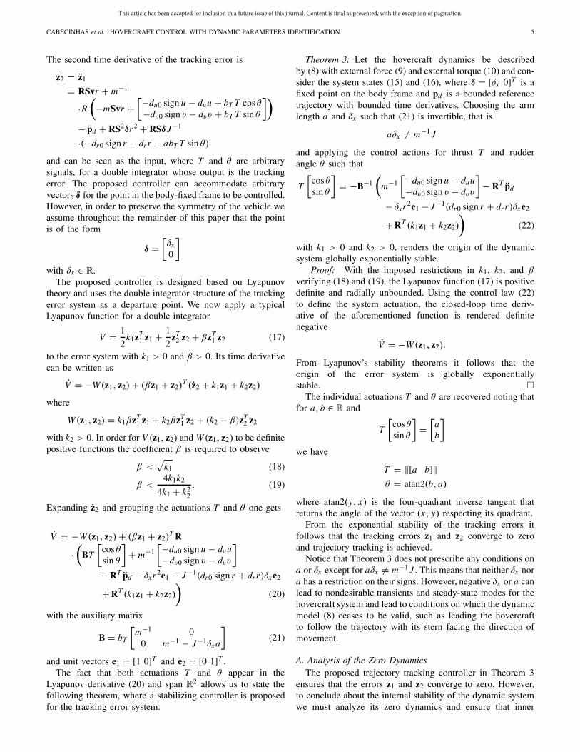
corresponding to a period of 2π s. A 2-D view of the referenceand hovercraft trajectories is shown in Fig. 2. After an initialtransient, the trajectory tracking performance is good andthe hovercraft is brought to the reference trajectory. Themodification of the simulation parameters at t = 15 s causesthe trajectory tracking error to increase and the hovercraftfollows an oval trajectory but with a larger radius than thereference, due to the mismatch between the parameters usedfor control and the actual parameters. Once the estimator isactive in closed loop, at t = 30s, the hovercraft immediatelysteers toward the desired reference trajectory, which it thenfollows closely.

V = −W (z1, z2) + (βz1 + z2)T R

[ζ−1

7 (ζ1 sign u + ζ2u)

(ζ7 − ζ8δx)−1(ζ3 sign v + ζ4v + ζ5 sign rδx + ζ6rδx)

](27)



Fig. 2. Position of the hovercraft and reference position. The initial positionsare marked with an ×.

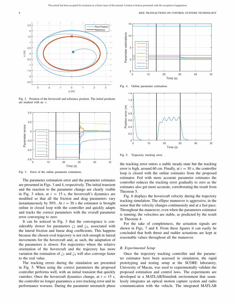
Fig. 3. Error of the online parameter estimation.

The parameter estimation error and the parameter estimatesare presented in Figs. 3 and 4, respectively. The initial transientand the reaction to the parameter change are clearly visiblein Fig. 3 when, at t = 15 s, the hovercraft’s dynamics aremodified so that all the friction and drag parameters varyinstantaneously by 50%. At t = 30 s the estimator is broughtonline in closed loop with the controller and quickly adaptsand tracks the correct parameters with the overall parametererror converging to zero.

It can be noticed in Fig. 3 that the convergence is con-siderably slower for parameters ζ3 and ζ4, associated withthe lateral friction and linear drag coefficients. This happensbecause the chosen oval trajectory is not rich enough in lateralmovements for the hovercraft and, as such, the adaptation ofthe parameters is slower. For trajectories where the relativeorientation of the hovercraft and the trajectory has morevariation the estimation of ζ3 and ζ4 will also converge fasterto the real value.

The tracking errors during the simulation are presentedin Fig. 5. When using the correct parameters the proposedcontroller performs well, with an initial transient that quicklyvanishes. Once the hovercraft dynamics change, at t = 15 s,the controller no longer guarantees a zero tracking error and itsperformance worsens. During the parameter mismatch phase

Fig. 4. Online parameter estimation.

Fig. 5. Trajectory tracking error.

the tracking error enters a stable steady-state but the trackingerror is high, around 60 cm. Finally, at t = 30 s, the controllerloop is closed with the online estimates from the proposedestimator. Fed with more accurate parameter estimates thecontroller reduces the tracking error gradually to zero as theestimates also get more accurate, corroborating the result fromTheorem 5.

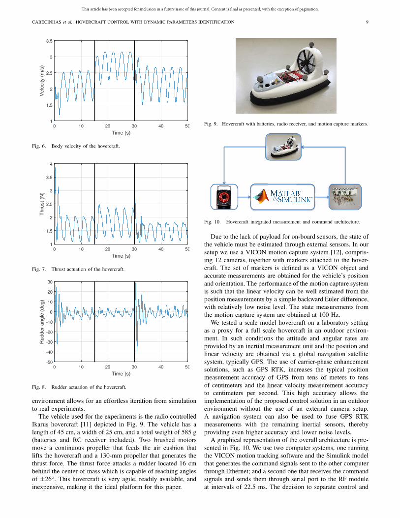
Fig. 6 displays the hovercraft velocity during the trajectorytracking simulation. The ellipse maneuver is aggressive, in thesense that the velocity changes continuously and at a fast pace.Throughout the maneuver, even when the parameters estimatoris running, the velocities are stable, as predicted by the resultin Theorem 4.

For the sake of completeness, the actuation signals areshown in Figs. 7 and 8. From these figures it can easily beconcluded that both thrust and rudder actuations are kept atreasonable values throughout all the maneuver.

B. Experimental Setup

Once the trajectory tracking controller and the parame-ter estimator have been assessed in simulation, the rapidprototyping and testing setup at the SCORE laboratory,University of Macau, was used to experimentally validate theproposed estimation and control laws. The experiments aredeveloped in a MATLAB/Simulink environment that seam-lessly integrates an optical motion capture system and radiocommunication with the vehicle. The integrated MATLAB



Fig. 6. Body velocity of the hovercraft.

Fig. 7. Thrust actuation of the hovercraft.

Fig. 8. Rudder actuation of the hovercraft.

environment allows for an effortless iteration from simulationto real experiments.

The vehicle used for the experiments is the radio controlledIkarus hovercraft [11] depicted in Fig. 9. The vehicle has alength of 45 cm, a width of 25 cm, and a total weight of 585 g(batteries and RC receiver included). Two brushed motorsmove a continuous propeller that feeds the air cushion thatlifts the hovercraft and a 130-mm propeller that generates thethrust force. The thrust force attacks a rudder located 16 cmbehind the center of mass which is capable of reaching anglesof ±26◦. This hovercraft is very agile, readily available, andinexpensive, making it the ideal platform for this paper.

Fig. 9. Hovercraft with batteries, radio receiver, and motion capture markers.

Fig. 10. Hovercraft integrated measurement and command architecture.

Due to the lack of payload for on-board sensors, the state ofthe vehicle must be estimated through external sensors. In oursetup we use a VICON motion capture system [12], compris-ing 12 cameras, together with markers attached to the hover-craft. The set of markers is defined as a VICON object andaccurate measurements are obtained for the vehicle’s positionand orientation. The performance of the motion capture systemis such that the linear velocity can be well estimated from theposition measurements by a simple backward Euler difference,with relatively low noise level. The state measurements fromthe motion capture system are obtained at 100 Hz.

We tested a scale model hovercraft on a laboratory settingas a proxy for a full scale hovercraft in an outdoor environ-ment. In such conditions the attitude and angular rates areprovided by an inertial measurement unit and the position andlinear velocity are obtained via a global navigation satellitesystem, typically GPS. The use of carrier-phase enhancementsolutions, such as GPS RTK, increases the typical positionmeasurement accuracy of GPS from tens of meters to tensof centimeters and the linear velocity measurement accuracyto centimeters per second. This high accuracy allows theimplementation of the proposed control solution in an outdoorenvironment without the use of an external camera setup.A navigation system can also be used to fuse GPS RTKmeasurements with the remaining inertial sensors, therebyproviding even higher accuracy and lower noise levels.

A graphical representation of the overall architecture is pre-sented in Fig. 10. We use two computer systems, one runningthe VICON motion tracking software and the Simulink modelthat generates the command signals sent to the other computerthrough Ethernet; and a second one that receives the commandsignals and sends them through serial port to the RF moduleat intervals of 22.5 ms. The decision to separate control and



TABLE II

PARTITION OF THE EXPERIMENTAL TEST

communications was made to avoid jitter in the transmission ofthe serial-port signals to the RF module, which occurs whenrunning all the systems in the same computer, and leads toerratic communication with the vehicle.

C. Closed-Loop Estimation and Control

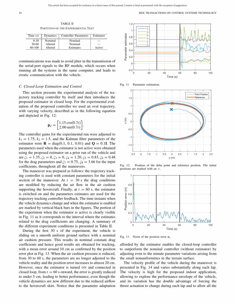
This section presents the experimental analysis of the tra-jectory tracking controller by itself and then introduces theproposed estimator in closed loop. For the experimental eval-uation of the proposed controller we used an oval trajectory,with varying velocity, described as in the following equationand depicted in Fig. 12:

pd =[

1.15 cos(0.7t)2.00 sin(0.7t)

].

The controller gains for the experimental run were adjusted tok1 = 1.75, k2 = 1.5, and the Kalman filter parameters of theestimator were R = diag(0.1, 0.1, 0.01) and Q = 0.1I. Theparameters used when the estimator is not active were obtainedusing the proposed estimator on a prior run of the vehicle andare ζ1 = 1.35, ζ2 = 0, ζ3 = 0, ζ4 = 1.20, ζ5 = 0.83, ζ6 = 0.48for the drag parameters and ζ7 = 0.75, ζ8 = 3.66 for the inputcoefficients, throughout all the maneuvers.

The maneuver was prepared as follows: the trajectory track-ing controller is used with constant parameters for the initialsection of the maneuver. At t = 30 s the drag conditionsare modified by reducing the air flow in the air cushionsupporting the hovercraft. Finally, at t = 60 s, the estimatoris switched on and the parameters estimates are used for thetrajectory tracking controller feedback. The time instants whenthe vehicle dynamics change and when the estimator is enabledare marked by vertical black bars in the figures. The portion ofthe experiment when the estimator is active is clearly visiblein Fig. 11 as it corresponds to the interval where the estimatesrelated to the drag coefficients are changing. A summary ofthe different experiment conditions is presented in Table II.

During the first 30 s of the experiment, the vehicle issliding on a smooth uniform ground surface with a nominalair cushion pressure. This results in nominal constant dragcoefficients and hence good results are obtained for tracking,with a mean error around 10 cm as confirmed by the positionerror plot in Fig. 13. When the air cushion pressure is reduced,from 30 to 60 s, the parameters are no longer adjusted to thevehicle reality and the position error increases to almost 20 cm.However, once the estimator is turned ON and connected inclosed loop, from t = 60 s onward, the error is greatly reducedto under 5 cm, leading to better performance, even though thevehicle dynamics are now different due to the reduced airflowto the hovercraft skirt. Notice that the parameter adaptation

Fig. 11. Parameter estimation.

Fig. 12. Position of the delta point and reference position. The initialpositions are marked with an ×.

Fig. 13. Norm of the position error z1.

afforded by the estimator enables the closed-loop controllerto outperform the nominal controller (without estimator) byadjusting even to the minute parameter variations arising fromthe small nonuniformities in the terrain surface.

The velocity profile of the vehicle during the maneuver ispresented in Fig. 14 and varies substantially along each lap.The velocity is high for the proposed indoor application,allowing to explore the performance envelope of the vehicle,and its variation has the double advantage of forcing thethrust actuation to change during each lap and to allow all the



Fig. 14. Velocity profile of the trajectory.

Fig. 15. Hovercraft’s yaw angle and yaw rate.

Fig. 16. Rudder actuation of the hovercraft.

parameters to be estimated since a changing velocity excitesmore of the estimator modes and makes the observabilityGrammian matrix positive definite.

The evolutions of the yaw angle and the respective rate,as well as the corresponding control actuation are shownin Figs. 15 and 16. The periodicity of the maneuver is clearlyvisible with the only exception being the initial transientwhen the vehicle is not close to the desired trajectory. Theaxis symmetry of the desired elliptical trajectory can also beobserved in Fig. 15. During a complete lap (yaw angle chang-ing by 360◦) it can be noticed that the yaw rate comes close tozero twice and has two peaks. This cyclic change correspondsto the vehicle steering along the ellipse alternating between

Fig. 17. Thrust actuation of the hovercraft.

moving along the long axis (lower curvature, lower yaw rate)and short axis (larger curvature, larger yaw rate). The evolutionof the rudder angle follows closely the yaw rate, but withopposite signs, since large changes in heading require largerudder angles. The physical rudder angle saturates at ±26◦,which is seldom attained.

The thrust command was identified by the current thepropeller motor draws when running. The current is linearlyrelated with the generated thrust force by the scaling coeffi-cient bT which is computed by the estimator. The thrust alsoevolves periodically and the commanded actuation, as seenin Fig. 17, is almost always below the physical motor limita-tion current of 6.1 A. Even in the nonideal conditions whenthe control parameters do not match reality both actuationsare reasonably within their saturation limits and do not differmuch from the nominal actuations. The higher periodic spikesin T , as well as the two outliers above 6.1 A, correspond tonoisy measurements due to the vehicle crossing a region whereit is less visible by the VICON motion capture system and themeasurements are ill-conditioned and especially noisy.

It should also be noticed that the proposed controller is ableto handle the measurement noise. The position and angle mea-surements are obtained by an optical motion capture systemresulting in noise levels that are relatively low and comparable,at the same scale, with measurement noise from RTK GPS andattitude measurements obtained from an attitude and headingreference system. However, measurement noise is noticeablein the velocity states measurements, plotted in Figs. 14 and 15,since they are determined by a finite difference approximationwherein the high frequency noise is amplified.

IX. CONCLUSION

This paper presented an integrated parameter estimator andtrajectory tracking controller for a nonholonomic hovercraft.A parameter estimator for generic time-varying systems thatare linear in the unknown parameters was devised and thenparticularized for the vehicle at hand in order to estimate theunknown parameters related to the drag forces, inputs, mass,and inertia. A trajectory tracking controller was proposedfor the hovercraft, which makes a fixed point in the bodyframe follow a predefined trajectory. The tracking error systemis exponentially stable and its zero dynamics are stable.



Furthermore, the closed-loop interconnection of the estimatorand controller was deemed to be locally asymptotically stable.The experimental results attested the stability of the intercon-nection as well as the performance and robustness of the pro-posed solution. The experimental results also corroborate thatthe introduction of the closed-loop parameter estimator greatlyreduces the trajectory tracking error in non-nominal conditionswithout any adverse side effects. This greatly increases theperformance of this kind of vehicle, which has the ability tomove on very different surfaces that can drastically change thevehicle drag profile.

REFERENCES

[1] I. Fantoni, R. Lozano, F. Mazenc, and K. Y. Pettersen, “Stabilization of anonlinear underactuated hovercraft,” in Proc. 38th IEEE Conf. DecisionControl, vol. 3. Dec. 1999, pp. 2533–2538.

[2] W. B. Dunbar, R. O. Saber, and R. M. Murray, “Nonlinear andcooperative control of multiple hovercraft with input constraints,” inProc. IEEE Eur. Control Conf., Sep. 2003, pp. 1917–1922.

[3] A. P. Aguiar, L. Cremean, and J. P. Hespanha, “Position tracking for anonlinear underactuated hovercraft: Controller design and experimentalresults,” in Proc. 42nd IEEE Conf. Decision Control, vol. 4, Dec. 2003,pp. 3858–3863.

[4] K. Tanaka, M. Iwasaki, and H. O. Wang, “Switching control of an R/Chovercraft: Stabilization and smooth switching,” IEEE Trans. Syst., Man,Cybern. B, Cybern., vol. 31, no. 6, pp. 853–863, Dec. 2001.

[5] A. Stubbs, V. Vladimerou, A. T. Fulford, D. King, J. Strick, andG. E. Dullerud, “Multivehicle systems control over networks: A hov-ercraft testbed for networked and decentralized control,” IEEE ControlSyst., vol. 26, no. 3, pp. 56–69, Jun. 2006.

[6] R. Munoz-Mansilla, D. Chaos, J. Aranda, and J. M. Diaz, “Applicationof quantitative feedback theory techniques for the control of a non-holonomic underactuated hovercraft,” IET Control Theory Appl., vol. 6,no. 14, pp. 2188–2197, Sep. 2012.

[7] P. Batista, C. Silvestre, and P. Oliveira, “Single range aided navigationand source localization: Observability and filter design,” Syst. ControlLett., vol. 60, no. 8, pp. 665–673, Aug. 2011.

[8] S. S. Sastry and C. A. Desoer, “The robustness of controllabilityand observability of linear time-varying systems,” IEEE Trans. Autom.Control, vol. 27, no. 4, pp. 933–939, Aug. 1982.

[9] A. Jazwinski, “Stochastic processes and filtering theory,” in Math-ematics in Science and Engineering. Amsterdam, The Netherlands:Elsevier, 1970. [Online]. Available: https://books.google.co.uk/books?id=nGlSNvKyY2MC

[10] H. K. Khalil, Nonlinear Systems, 2nd ed. Englewood Cliffs, NJ, USA:Prentice-Hall, 1996.

[11] Ikarus. Dragstair Hovercraft Instruction Manual and Specifications.[Online]. Available: http://www.ikarus.net/download/anleitungen/Hovercrafts/Dragstair/dragstair_anleitung_3sprachig_incl_konformitt.pdf

[12] VICON. [Online]. Available: http://www.vicon.com

David Cabecinhas received the Licenciatura andPh.D. degrees in electrical and computer engineeringfrom the Instituto Superior Técnico, Lisbon, Portu-gal, in 2006 and 2014, respectively.

He has been a Researcher with the Institute forSystems and Robotics, LarSyS, Lisbon, since 2007.He is currently a Post-Doctoral Fellow with theFaculty of Science and Technology, University ofMacau, Macau, China. His current research interestsinclude nonlinear control, sensor-based and vision-based control with applications to autonomous aerial

and surface vehicles, and the modeling and identification of aerial and surfacevehicles.

Pedro Batista (M’10) received the Licenciaturadegree in electrical and computer engineering in2005 and the Ph.D. degree from the Instituto Supe-rior Técnico (IST), Lisbon, Portugal, in 2005 and2010, respectively.

From 2004 to 2006, he was a Monitor with theDepartment of Mathematics, IST. Since 2012, hehas been with the Department of Electrical andComputer Engineering, IST, where he is currentlyan Assistant Professor. His current research interestsinclude sensor-based navigation and the control of

autonomous vehicles.Dr. Batista has received the Diploma de Mérito twice during his graduation

and his Ph.D. dissertation was awarded the Best Robotics Ph.D. Thesis Awardby the Portuguese Society of Robotics.

Paulo Oliveira (S’91–M’95–SM’11) received theLicenciatura, M.Sc., and Ph.D. degrees in electricaland computer engineering from the Instituto Supe-rior Técnico (IST), Lisbon, Portugal, in 1987, 1991,and 2002, respectively.

Since 2012, he has been an Associate Professorwith the Department of Mechanical Engineering,IST. He has authored or co-authored over 65 journalpapers and 180 conference communications. He hasparticipated in more than 30 European and Por-tuguese research projects, over the last 25 years.

His current research interests include autonomous robotic vehicles with afocus on the fields of estimation, sensor fusion, navigation, positioning, andmechatronics.

Carlos Silvestre (M’05) received the Licenciaturaand M.Sc. degrees in electrical engineering, thePh.D. degree in control science, and the Habilitationdegree in electrical engineering and computers fromthe Instituto Superior Técnico (IST), Lisbon, Portu-gal, in 1987, 1991, 2000, and 2011, respectively.

Since 2000, he has been with the Department ofElectrical Engineering, IST, where he is currentlyan Associate Professor of Control and Robotics,on leave. Since 2015, he has been a Professorwith the Department of Electrical and Computers

Engineering, Faculty of Science and Technology, University of Macau, Macau,China. Over the past years, he has conducted research on the subjects of thenavigation guidance and control of air and underwater robots. His currentresearch interests include linear and nonlinear control theory, the coordinatedcontrol of multiple vehicles, gain scheduled control, the integrated design ofguidance and control systems, inertial navigation systems, and mission controland real-time architectures for complex autonomous systems with applicationsto unmanned air and underwater vehicles.

Documents

IEEE TRANSACTIONS ON CONTROL SYSTEMS TECHNOLOGY 1 ...welcome.isr.tecnico.ulisboa.pt/wp-content/uploads/... · structure (1) we consider a hovercraft, an underactuated dynamic system,