IEEE TRANSACTIONS ON COMPUTERS, VOL.54, …cs.txstate.edu/~burtscher/papers/tc05.pdfThe VPC Trace-Compression Algorithms Martin Burtscher, Member, IEEE, Ilya Ganusov, Student Member,

The VPC Trace-Compression AlgorithmsMartin Burtscher, Member, IEEE, Ilya Ganusov, Student Member, IEEE, Sandra J. Jackson,

Jian Ke, Paruj Ratanaworabhan, and Nana B. Sam, Student Member, IEEE

Abstract—Execution traces, such as are used to study and analyze program behavior, are often so large that they need to be stored in

compressed form. This paper describes the design and implementation of four value prediction-based compression (VPC) algorithms

for traces that record the PC as well as other information about executed instructions. VPC1 directly compresses traces using value

predictors, VPC2 adds a second compression stage, and VPC3 utilizes value predictors to convert traces into streams that can be

compressed better and more quickly than the original traces. VPC4 introduces further algorithmic enhancements and is automatically

synthesized. Of the 55 SPECcpu2000 traces we evaluate, VPC4 compresses 36 better, decompresses 26 faster, and compresses 53

faster than BZIP2, MACHE, PDATS II, SBC, and SEQUITUR. It delivers the highest geometric-mean compression rate,

decompression speed, and compression speed because of the predictors’ simplicity and their ability to exploit local value locality. Most

other compression algorithms can only exploit global value locality.

Index Terms—Data compaction and compression, performance analysis and design aids.

�

1 INTRODUCTION

EXECUTION traces are widely used in industry andacademia to study the behavior of programs and

processors. The problem is that traces from interestingapplications tend to be very large. For example, collectingjust one byte of information per executed instructiongenerates on the order of a gigabyte of data per second ofCPU time on a high-end microprocessor. Moreover, tracesfrom many different programs are typically collected tocapture a wide variety of workloads. Storing the resultingmultigigabyte traces can be a challenge, even on today’slarge hard disks.

One solution is to regenerate the traces every time theyare needed instead of saving them. For example, tools likeATOM [11], [44] can create instrumented binaries thatproduce a trace every time they are executed. However,execution-driven approaches are ISA specific and, thus,hard to port, produce nonrepeatable results for nondeter-ministic programs, and are undesirable in situations wheretrace regeneration is impossible, too expensive, or too slow.

An alternative solution is to generate the traces once andto store them (in compressed form). The disadvantage ofthis approach is that it requires disk space and that thetraces must be decompressed before they can be used. TheVPC trace compression algorithms presented in this paperaim at minimizing these downsides.

To be useful, a trace compressor has to provide severalbenefits in addition to a good compression rate and a fastdecompression speed. For example, a fast compressionspeed may also be desirable. Moreover, lossless compres-sion is almost always required so that the original trace canbe reconstructed precisely. A constant memory footprintguarantees that a system can handle even the largest andmost complicated traces. Finally, a single-pass algorithm isnecessary to ensure that the large uncompressed trace never

has to exist in its entirety because it can be compressed as itis generated and decompressed as simulators or other toolsconsume it. VPC3 [4] and VPC4 [6], our most advancedalgorithms, possess all these qualities.

Many trace-compression algorithms have been proposed[2], [4], [10], [15], [16], [23], [24], [25], [28], [29], [32], [33],[38], [41], [48]. Most of them do an excellent job atcompressing program traces that record the PCs of executedinstructions (PC traces) or the addresses of memory accesses(address traces). However, extended traces that contain PCsplus additional information, such as the content of registers,values on a bus, or even filtered address sequences, areharder to compress because such data repeat less often,exhibit fewer patterns, or span larger ranges than the entriesin PC and address traces. Yet, such traces are gainingimportance as more and more researchers investigate thedynamic activities in computer systems. We designed theVPC algorithms [4], [5], [6] especially for extended traces.

A comparison with SEQUITUR [29] and SBC [33], two ofthe best trace-compression algorithms in the currentliterature, on the three types of traces we generated fromthe SPECcpu2000 programs yielded the following results.On average (geometric mean), VPC4 outperforms SBC by79 percent in compression rate, 1,133 percent in compres-sion time, and 25 percent in decompression time on PC plusstore-address traces and by 88 percent in compression rate,850 percent in compression time, and 27 percent indecompression time on PC plus load-value traces. Itoutperforms SEQUITUR on average by 1,356 percent incompression rate, 668 percent in compression time, and36 percent in decompression time on the PC plus store-address traces and by 105 percent in compression rate,535 percent in compression time, and 6 percent indecompression time on the PC plus load-value traces.Section 6 presents more results.

The VPC algorithms all have a set of value predictors attheir core. Value predictors identify patterns in valuesequences and extrapolate those patterns to forecast thelikely next value. In recent years, hardware-based valuepredictors have been researched extensively to predict thecontent of CPU registers [7], [8], [13], [14], [31], [40], [43], [45],[47]. Since these predictors are designed to make billions of

IEEE TRANSACTIONS ON COMPUTERS, VOL. 54, NO. 11, NOVEMBER 2005 1

. The authors are with the Computer Systems Laboratory, School ofElectrical and Computer Engineering, Cornell University, Ithaca, NY14853. E-mail: {burtscher, ilya, sandra, jke, paruj, besema}@csl.cornell.edu.

Manuscript received 9 Aug. 2004; revised 18 Feb. 2005; accepted 6 June 2005;published online 16 Sept. 2005.For information on obtaining reprints of this article, please send e-mail to:[email protected], and reference IEEECS Log Number TC-0265-0804.

0018-9340/05/$20.00 � 2005 IEEE Published by the IEEE Computer Society

predictions per second, they use simple and fast algorithms.Moreover, they are good at predicting the kind of valuestypically found in program traces, such as jump targets,effective addresses, etc., because such values are stored inregisters. These features make value predictors great candi-dates for our purposes. In fact, sincewe are implementing thepredictors in software,we canusemore predictors and largertables than are feasible in a hardware implementation,resulting in even more accurate predictions.

The following simple example illustrates how valuepredictors can be used to compress traces. Let us assumethat we have a set of predictors and that our trace containseight-byte entries. During compression, the current traceentry is compared with the predicted values. If at least one ofthe predictions is correct, we write only the identificationcode of one of the correct predictors to the output, encoded inaone-byte value. If noneof thepredictions are right,we emit aone-byte flag followed by the unpredictable eight-byte traceentry. Then, the predictors are updated and the procedurerepeats until all trace entries have been processed. Note thatthe output of this algorithm should be further compressed,e.g., with a general-purpose compressor.

Decompression proceeds analogously. First, one byte isread from the compressed input. If it contains the flag, thenext eight bytes are read to obtain the unpredictable traceentry. If, on the other hand, the byte contains a predictoridentification code, the value from that predictor is used.Then, the predictors are updated to ensure that their state isconsistent with the corresponding state during compres-sion. This process iterates until the entire trace has beenreconstructed.

VPC1 essentially embodies the above algorithm. It uses37 value predictors, compresses the predictor identificationcodes with a dynamic Huffman encoder, and employs aform of differential encoding to compress the unpredictabletrace entries [5]. VPC1 delivers good compression rates onhard-to-compress extended traces, but is not competitive onother kinds of traces.

As it turns out, VPC1’s output itself is quite compres-sible. Thus, VPC2 improves upon VPC1 by adding anadditional compression stage [5]. It delivers good compres-sion rates on hard-to-compress as well as simple extendedtraces. Unfortunately, VPC2’s decompression speed isalmost four times slower than that of other algorithms.

VPC3 capitalizes on the fact that extended traces aremore compressible after processing them with valuepredictors. Hence, we changed the purpose of the valuepredictors from compressing the traces to converting theminto streams that a general-purpose compressor can quicklycompress well [4]. Using the value predictors in this manneris more fruitful than using them for the actual compression,as the compression rates and speeds in Section 6 show.

VPC4 adds several algorithmic enhancements to make itfaster and to improve the compression rate. Moreover, it isnot handcrafted like its predecessors. Instead, it is synthe-sized out of a simple description of the trace format and thepredictors to be used [6].

Most data compressors are comprised of two generalcomponents, one to recognize patterns and the other toencode a representation of these patterns into a smallnumber of bits. The VPC algorithms fit this standardcompression paradigm, where the value predictors repre-sent the first component and the general-purpose compres-sor represents the second. The innovation is the use of valuepredictors as pattern recognizers, which results in a power-ful trace compressor for the following reason. Extended

traces consist of records with a PC field and at least oneextended data (ED) field. The value predictors separate thedata component of extended traces into ministreams, onefor each distinct PC (modulo the predictor size). In otherwords, the prediction of the next ED entry is not based onthe immediately preceding n trace entries, but on thepreceding n entries with the same PC. This allows VPC tocorrelate data from one instruction with data that that sameinstruction produced rather than with data from “nearby”but otherwise unrelated instructions. As a result, theministreams exhibit more value locality than the originaltrace in which the data are interleaved in complicated ways.The VPC algorithms are thus able to detect and exploitpatterns that other compressors cannot, which explainsVPC’s performance advantage on extended traces. Notethat the value predictors are essential because they caneasily handle tens of thousands of parallel ministreams.While other algorithms could also split the traces intoministreams, it would be impractical, for example, tosimultaneously run ten thousand instances of BZIP2 or toconcurrently generate ten thousand grammars in SEQUI-TUR. Nevertheless, Zhang and Gupta have been able toimprove the compression rate of SEQUITUR by taking astep in this direction. They generate a subtrace for eachfunction and then compress the subtraces individually [49].

The C source code of VPC3 is available online athttp://www.csl.cornell.edu/~burtscher/research/tracecompression/. A sample test trace and a brief descriptionof the algorithm are also included. TCgen, the tool thatgenerated VPC4, is available at http://www.csl.cornell.edu/~burtscher/research/TCgen/. The code has beensuccessfully tested on 32 and 64-bit Unix and Linux systemsusing cc and gcc as well as on Windows under cygwin [19].

The remainder of this paper is organized as follows:Section 2 summarizes related work. Section 3 introducesour trace format and the value predictors VPC uses.Section 4 describes the four VPC algorithms in detail.Section 5 presents the evaluation methods. Section 6explains the results, and Section 7 concludes the paper.

2 RELATED WORK

A large number of compression algorithms exist. Due tospace limitations, we mainly discuss lossless algorithmsthat have been specifically designed to compress traces. Thealgorithms we evaluate in the result section are described inSection 2.2.

VPC shares many ideas with the related work describedin this section. For example, it exploits sequentiality andspatiality, predicts values, separates streams, matchespreviously seen sequences, converts absolute values intooffsets, and includes a second compression stage.

2.1 Compression Approaches

Larus proposed Abstract Execution (AE) [28], a systemdesigned mainly for collecting traces of memory addressesand data. AE starts by instrumenting the program to betraced. However, instead of instrumenting it to collect a fulltrace, it only collects significant events (SE). AE thengenerates and compiles a program that creates the completetrace out of the SE data. Normally, the SE trace size is muchsmaller than the size of the full trace and the cost of runningthe program to collect the SEs is much lower than the cost ofrunning the program to collect the complete trace. The AEsystem is language and platform specific.

2 IEEE TRANSACTIONS ON COMPUTERS, VOL. 54, NO. 11, NOVEMBER 2005

PDATS [24] compresses address traces in which areference type (data read, data write, or instruction fetch)distinguishes each entry. It converts the absolute addressesinto offsets, which are the differences between successivereferences of the same type, and uses the minimum numberof bytes necessary to express each offset. Each entry in theresulting PDATS file consists of a header byte followed by avariable-length offset. The header byte includes the refer-ence type, the number of bytes in the offset, and a repeatcount. The repeat count is used to encode multiplesuccessive references of the same type and offset. Theresult is fed into a second compressor.

Pleszkun designed a two-pass algorithm to compresstraces of instruction and data addresses [38]. The first passpartially compresses the trace, generates a collection of datastructures, and records the dynamic control flow of theoriginal program. During the second pass, this informationis used to encode the dynamic basic block successors andthe data offsets using a compact representation. At the end,the output is passed through a general-purpose compressor.

To handle access pattern irregularities in address tracesdue to, for example, operating system calls or contextswitches, Hammami [15] proposes to first group theaddresses in a trace into clusters using machine-learningtechniques. Then, the “mean” of each cluster is computed.This mean forms the base address for that cluster. Finally,the addresses within each cluster are encoded as offsets tothe corresponding base address. This approach can be used,for instance, on top of PDATS, but increases the number ofpasses over the trace.

Address Trace Compression through Loop Detectionand Reduction [10] is a multipass algorithm that is gearedtoward address traces of load/store instructions. Thiscompression scheme is divided into three phases. In thefirst phase, control-flow analysis techniques are used toidentify loops in the trace. In the second phase, the addressreferences within the identified loops are grouped into threetypes: 1) constant references, which do not change from oneiteration to the next, 2) loop varying references, whichchange by a constant offset between consecutive iterations,and 3) chaotic references, which do not follow anydiscernible patterns. In the last phase, the first two typesof address references are encoded while the third type is leftunchanged.

Johnson et al. introduce the PDI technique [25], which isan extension of PDATS for compressing traces that containinstruction words in addition to addresses. In PDI,addresses are compressed using the PDATS algorithm,while the instruction words are compressed using adictionary-based approach. The PDI file contains a dic-tionary of the 256 most common instruction words found inthe trace, which is followed by variable length records thatencode the trace entries. Identifying the most frequentinstruction words requires a separate pass over the trace.PDI employs a general-purpose compressor to boost thecompression rate.

Ahola proposes RECET [1], a hardware and softwareplatform to capture and process address traces and toperform cache simulations in real-time. RECET first sendsthe traces through a small cache to filter out hits, stores theremaining data in the MACHE format, and furthercompresses them with the Lempel-Ziv method [50]. Theresulting traces can be used to simulate caches with linesizes and associativities that are equal to or larger than thatof the filter cache.

Hamou-Lhadj and Lethbridge [16] use common sub-expression elimination to compress procedure-call traces.The traces are represented as trees and subtrees that occurrepeatedly are eliminated by noting the number of timeseach subtree appears in the place of the first occurrence. Adirected acyclic graph is used to represent the order inwhich the calls occur. This method requires a preprocessingpass to remove simple loops and calls generated byrecursive functions. One benefit of this type of compressionis that it can highlight important information contained inthe trace, thus making it easier to analyze.

STEP [2] provides a standard method of encodinggeneral trace data to reduce the need for developers toconstruct specialized systems. STEP uses a definitionlanguage designed specifically to reuse records and feeddefinition objects to its adaptive encoding process, whichemploys several strategies to increase the compressibility ofthe traces. The traces are then compressed using a general-purpose compressor. STEP is targeted toward applicationand compiler developers and focuses on Java programsrunning on JVMs.

The Locality-Based Trace Compression algorithm [32]was designed to exploit the spatial and temporal locality in(physical) address traces. It is similar to PDATS except itstores all attributes that accompany each memory reference(e.g., the instruction word or the virtual address) in a cachethat is indexed by the address. When the attributes in theselected cache entry match, a hit bit is recorded in thecompressed trace. In case of a cache miss, the attributes arewritten to the compressed trace. This caching captures thetemporal locality of the memory references.

Several papers point out or exploit the close relationshipbetween prediction and compression. For example, Chenet al. [9] argue that a two-level branch predictor is anapproximation of the optimal PPM predictor and hypothe-size that data compression provides an upper limit on theperformance of correlated branch prediction. While we useprediction techniques to improve compression, Federovskyet al. [12] use compression methods to improve (branch)prediction.

2.2 Compression Algorithms

This section describes the compression schemes with whichwe compare our approach in Section 6. BZIP2 is a lossless,general-purpose algorithm that can be used to compressany kind of file. The remaining algorithms are special-purpose trace compressors that we modified to includeefficient block I/O operations and to include a secondcompression stage to improve the compression rate. Theyare all single-pass, lossless compression schemes that“know” about the PC and extended data fields in ourtraces. However, none of these algorithms separate theextended data into ministreams like VPC does.

BZIP2 [18] is quickly gaining popularity in the Unixworld. It is a general-purpose compressor that operates atbyte granularity. It implements a variant of the block-sorting algorithm described by Burrows and Wheeler [3].BZIP2 applies a reversible transformation to a block ofinputs, uses sorting to group bytes with similar contextstogether, and then compresses them with a Huffman coder.The block size is adjustable. We use the “–best” optionthroughout in this paper. According to ps, BZIP2 requiresabout 10MB of memory to compress and decompress ourtraces. We evaluate BZIP2 version 1.0.2 as a standalonecompressor and as the second stage compressor for all theother algorithms.

BURTSCHER ET AL.: THE VPC TRACE-COMPRESSION ALGORITHMS 3

MACHE [41] was primarily designed to compressaddress traces. It distinguishes between three types ofaddresses, namely, instruction fetches, memory reads, andmemory writes. A label precedes each address in the traceto indicate its type. After reading in a label and addresspair, MACHE compares the address with the current base.There is one base for each possible label. If the differencebetween the address and the base can be expressed in asingle byte, the difference is emitted directly. If thedifference is too large, the full address is emitted and thisaddress becomes the new base for the current label. Thisalgorithm repeats until the entire trace has been processed.

Our trace format is different from the standard MACHEformat. It consists of pairs of 32-bit PC and 64-bit dataentries. Since PC and data entries alternate, no labels arenecessary to identify their type. MACHE only updates thebase when the full address needs to be emitted. We retainthis policy for the PC entries. However, for the data entries,we found it better to always update the base due to thefrequently encountered stride behavior. Our implementa-tion uses 2.3MB of memory to run.

SEQUITUR [29], [35], [36], [37] is one of the mostsophisticated trace compression algorithms in the literature.It converts a trace into a context-free grammar and appliestwo constraints while constructing the grammar: Eachdigram (pair of consecutive symbols) in the grammar mustbe unique and every rule must be used more than once.SEQUITUR has the interesting feature that informationabout the trace can be derived from the compressed formatwithout having to decompress it first. The biggest drawbackof SEQUITUR is its memory usage, which depends on thedata to be compressed (it is linear in the size of thegrammar) and can exhaust the system’s resources whencompressing extended traces.

The SEQUITUR algorithm we use is a modified versionof Nevill-Manning and Witten’s implementation [17], whichwe changed as follows: We manually converted theC++ code into C, inlined the access functions, increasedthe symbol table size to 33,554,393 entries, and added codeto decompress the grammars. To accommodate 64-bit traceentries, we included a function that converts each traceentry into a unique number (in expected constant time).Moreover, we employ a split-stream approach, that is, weconstruct two separate grammars, one for the PC entriesand one for the data entries in our traces. To cap thememory usage, we start new grammars when eight millionunique symbols have been encountered or 384 megabytes ofstorage have been allocated for rule and symbol descriptors.We found these cutoff points work well on our traces andsystem. Our implementation’s memory usage never ex-ceeds 951MB, thus fitting into the 1GB of main memory inour system. To prevent SEQUITUR from becoming veryslow due to hash-table inefficiencies, we also start a newgrammar whenever the last 65,536 searches required anaverage of more than 30 trials before an entry was found.

PDATS II [23] improves upon PDATS by exploitingcommon patterns in program behavior. For example, jump-initiated sequences are often followed by sequentialsequences. PDATS encodes such patterns using one recordto specify the jump and another record to describe thesequential references. PDATS II combines the two recordsinto one. Moreover, when a program writes to a particularmemory location, it is also likely to read from that location.PDATS separates read and write references, resulting intwo large offsets whenever the location changes. To reducethe number of large offsets, PDATS II does not treat read

and write references separately. Additionally, common dataoffsets are encoded in the header byte and instructionoffsets are stored in units of the default instruction stride(e.g., four bytes per instruction on most RISC machines).Thus, PDATS II achieves about twice the compression rateof PDATS on average.

We modified PDATS II as follows: Since our traces donot include both read and write accesses, we do not need todistinguish between them in the header. This makes anextra bit available, which we use to expand the encodeddata offsets to include �16, �32, and �64. Because ourtraces contain offsets greater than 32 bits, we extendedPDATS II to also accommodate six and eight-byte offsets.Our traces do not exhibit many jump-initiated sequencesthat are followed by sequential sequences. Hence, we do notneed the corresponding PDATS II feature. Our implementa-tion uses 2.2MB of memory.

SBC (Stream-Based Compression) [33], [34] is one of thebest trace compressors in the literature. It splits traces intosegments called instruction streams. An instruction streamis a dynamic sequence of instructions from the target of ataken branch to the first taken branch in the sequence. SBCcreates a stream table that records relevant informationsuch as the starting address, the number of instructions inthe stream, and the instruction words and their types.During compression, groups of instructions in the originaltrace that belong to the same stream are replaced by thecorresponding stream table index. To compress addressesof memory references, SBC further records informationabout the strides and the number of stride repetitions. Thisinformation is attached to the instruction stream. Note thatVPC streams are unrelated to SBC streams as the formerspan the entire length of the trace.

We made the following changes to Milenkovics’ SBCcode [20]: Since our traces contain some but not allinstructions (e.g., only instructions that access the memory),we redefined the notion of an instruction stream as asequence in which each subsequent instruction has a higherPC than the previous instruction and the difference betweensubsequent PCs is less than a preset threshold. Weexperimented with different thresholds and found a thresh-old of four instructions to provide the best compression rateon our traces. SBC uses 10MB of memory to run.

3 BACKGROUND

3.1 Value Predictors

This section describes the operation of the value predictorsthat the various VPC algorithms use to predict trace entries.The exact predictor configurations are detailed in Sections 5.4and 5.5. All of the presented value predictors extrapolatetheir forecasts based on previously seen values, that is, theypredict the next trace entry based on already processedentries. Note that PC predictions are made based on globalinformation, while ED predictions are made based on localinformation, i.e., based on ministreams whose entries allhave the same PC.

Lastnvaluepredictor:The first typeof predictorVPCusesis the last n value predictor (LnV) [7], [30], [47]. It predicts themost likely value among the nmost recently seen values. Toimprove the compression rate, all n values are used (and notjust themost likely value), i.e., the predictor can be thought ofas comprising n components that make n independentpredictions. TheLnVpredictor accurately predicts sequencesof repeating and alternating values as well as repeatingsequences of no more than n arbitrary values. Since PCs


infrequently exhibit such behavior, the LnV predictor is onlyused for predicting data entries.

Stride 2-delta predictor: Stride predictors retain the mostrecently seen value along with the difference (stride)between the most recent and the second most recent values[13]. Adding this difference to the most recent value yieldsthe prediction. Stride predictors can therefore predictsequences of the following pattern:

A;AþB;Aþ 2B;Aþ 3B;Aþ 4B; . . . :

Every time a new value is seen, the difference and themost recent value in the predictor are updated. To improvethe prediction accuracy, the 2-delta method (ST2D) has beenproposed [43]. It introduces a second stride that is onlyupdated if the same stride is encountered at least twice in arow, thus providing some hysteresis before the predictorswitches to a new stride.

Finite context method predictor: The finite contextmethod predictor (FCMn) [43] computes a hash out of then most recently encountered values, where n is referred toas the order of the predictor. VPC utilizes the select-fold-shift-xor hash function [39], [40], [42]. During updates, thepredictor puts the new value into its hash table using thecurrent hash as an index. During predictions, a hash-tablelookup is performed in the hope that the next value will beequal to the value that followed last time the same sequenceof n previous values (i.e., the same hash) was encountered[42], [43]. Thus, FCMn predictors can memorize longarbitrary sequences of values and accurately predict themwhen they repeat. This trait makes FCMn predictors idealfor predicting PCs as well as EDs. Note that the hash table isshared among the ministreams, making it possible tocommunicate information from one ministream to another.

Differential finite context method predictor: The differ-ential finite context method predictor (DFCMn) [14] worksjust like the FCMnpredictor except it predicts and is updatedwith differences (strides) between consecutive values ratherthan with absolute values. To form the final prediction, thepredicted stride is added to the most recently seen value.DFCMn predictors are often superior to FCMn predictorsbecause they warm up faster, can predict never-before-seenvalues, and make better use of the hash table.

Global/local last value predictor: The global/local lastvalue predictor (GLLV) [5] works like the last-valuepredictor (i.e., like an LnV predictor with n ¼ 1), with theexception that each line contains two additional fields: anindex and a counter. The index designates which entry ofthe last-value table holds the prediction. The counterassigns a confidence to this index. Every time a correctprediction is made, the counter is set to its maximum andevery misprediction decrements it. If the counter is zero andthe indexed value incorrect, the counter is reset to themaximum and the index is incremented (modulo the tablesize) so that a different entry will be checked the next time.This way, the predictor is able to correlate any ministreamwith any other ministream without the need for multiplecomparisons per prediction or update.

3.2 Trace Format

The traces we generated for evaluating the differentcompression algorithms consist of pairs of numbers. Eachpair is comprised of a PC and an extended data (ED) field.The PC field is 32 bits wide and the data field is 64 bitswide. Thus, our traces have the following format, where thesubscripts indicate bit widths:

PC032;ED064;PC132;ED164;PC232;ED264; . . .:

This formatwas chosen for its simplicity.Weuse 64bits forthe ED fields because this is the nativeword size of theAlphasystem on which we performed our measurements. Thirty-two bits suffice to represent PCs, especially since we do notneed to store the two least significant bits, which are alwayszero because Alphas only support aligned instructions.

4 THE VPC ALGORITHMS

4.1 Prototype

The development of VPC started with a prototype of avalue-predictor-based compression algorithm that onlycompresses the extended data and works as follows. ThePC of the current PC/ED pair is copied to the output and isused to index a set of value predictors to produce 27 (notnecessarily distinct) predictions. The predicted values arethen compared to the ED. If a match is found, thecorresponding predictor identification code is written tothe output using a fixed m-bit encoding. If no prediction iscorrect, an m-bit flag is written followed by the unpredict-able 64-bit extended-data value. Then, the predictors areupdated with the true ED value. The algorithm repeats untilall PC/ED pairs in the trace have been processed.Decompression is essentially achieved by running thecompression steps in reverse.

This prototype algorithm is ineffective because it does notcompress the PCs and because m is too large. Since it uses27 predictors plus the flag, five bits are needed, i.e., m ¼ 5.Moreover, unpredictable ED entries are not compressed. Theprototype’s compression rate cannot exceed a factor of 2.6because, even assuming that every ED entry is predictable, a96-bit PC/ED pair (32-bit PC plus 64-bit ED) is merelycompressed down to 37 bits (a 32-bit PC plus a 5-bit code).

4.2 VPC1

VPC1 [5] corrects the shortcomings of the prototype. Itincludes a separate bank of 10 predictors to compress thePCs, bringing the total number of predictors to 37. It uses adynamic Huffman encoder [27], [46] to compress theidentification codes. If more than one predictor is correctsimultaneously, VPC1 selects the one with the shortestHuffman code. Moreover, it compresses the unpredictabletrace entries in the following manner: In case of PCs, onlyp bits are written, where p is provided by the user and hasto be large enough to express the largest PC in the trace. Incase of unpredictable ED entries, the flag is followed by theidentification code of the predictor whose prediction isclosest to the ED value in terms of absolute difference.VPC1 then emits the difference between the predicted valueand the actual value in compressed sign-magnitude format.

VPC1 includes several enhancements to boost thecompression rate. First, it incorporates saturating up/downcounters in the hash table of the FCMn predictors so thatonly entries that have proven useless at least twice in a rowcan be replaced. Second, it retains only distinct values in allof its predictors to maximize the number of differentpredictions and, therefore, the chance of at least one of thembeing correct. Third, it keeps the values in the predictors inleast recently used order. Due to the principle of valuelocality, sorting the values from most recent to least recentensures that components holding more recent values have ahigher probability of providing a correct prediction. Thisincreases the compression rate because it allows thedynamic Huffman encoder to assign shorter identificationcodes to the components holding more recent values and to


use them more often. Fourth, VPC1 initializes the dynamicHuffman encoder with biased, nonzero frequencies for allpredictors to allow the more sophisticated predictors, whichperform poorly in the beginning because they take longer towarm up, to stay ahead of the simpler predictors. Biasingthe frequencies guarantees that the most powerful pre-dictors are used whenever they are correct and theremaining predictors are only utilized occasionally, result-ing in shorter Huffman codes and better compression rates.

VPC1 only performs well on hard-to-compress traces [5].The problem is that its compression rate is limited to afactor of 48. Since at least one bit is needed to encode a PCand one bit to encode an extended-data entry and anuncompressed PC/ED pair requires 32þ 64 ¼ 96 bits, themaximum compression rate is 96=2 ¼ 48. We found VPC1to almost reach this theoretical maximum in several cases,showing that the dynamic Huffman encoder indeed oftenuses only one bit to encode a predictor identification code.Because the PC and ED predictor codes alternate in thecompressed traces and because at most one of the PCpredictors and one of the ED predictors can have a one-bitidentification code at any time, highly compressed VPC1traces contain long bit strings of all zeros, all ones, oralternating zeros and ones, depending on the two pre-dictors’ identification codes. As a result, compressed VPC1traces can be compressed further.

4.3 VPC2

VPC2 exploits the compressibility in VPC1’s output byadding a second compression stage. In other words, VPC2is VPC1 plus GZIP [21]. VPC2 outperforms VPC1 in allstudied cases [5]. More importantly, VPC2 also outperformsother algorithms, including SEQUITUR, on easy-to-com-press traces. Unfortunately, it is over 3.5 times slower atdecompressing traces.

4.4 VPC3

Analyzing the performance of VPC2, we noticed thatcompressing traces as much as possible with the valuepredictors often obfuscates patterns and makes the result-ing traces less amenable to the second stage compressor. Infact, we found that compressing less in the first stage canspeed up the algorithm and boost the overall compressionrate at the same time. Hence, we designed VPC3 to optimizethis interaction between the two stages, i.e., instead ofmaximizing the performance of each stage individually, wemaximized the overall performance. Thus, VPC3’s valuepredictors ended up only compressing the traces by a factorof between 1.4 to close to six (6.0 being the maximumpossible) before they are sent to the second stage.

VPC3 differs from VPC2 in the following ways: Wefound that removing infrequently used predictors decreasesthe number of distinct predictor codes and increases theregularity of the emitted identification codes, which resultsin better compression rates despite the concomitant increasein the number of emitted unpredictable values. As a result,VPC3 incorporates only 4 instead of 10 PC predictors andonly 10 instead of 27 data predictors. Similarly, wediscovered that abolishing the saturating counters andupdating with nondistinct values decreases the predictionaccuracy somewhat, but greatly accelerates the algorithm.Moreover, emitting values at byte granularity and, thus,possibly including unnecessary bits increases the amount ofdata transferred from the first to the second stage, butexposes more patterns and makes them easier to detect forthe second stage, which also operates at byte granularity.

Thus, VPC3 functions exclusively at byte granularity (andinteger multiples thereof), which further simplified andaccelerated the code. Finally, VPC3 does not use afrequency bias or a dynamic Huffman coder because thesecond stage is more effective at compressing the predictoridentification codes. For the same reason, unpredictablevalues are no longer compressed in the first stage, whichhas the pleasant side effect of eliminating the need for thenumber of bits (p) required to express the PCs in the trace.

Note that we investigated many more ideas but endedup implementing only the ones listed above because theyincrease the overall compression rate and accelerate thealgorithm. The following is a summary of some of ourexperiments that turned out to be disadvantageous. Theyare not included in VPC3.

1. The order in which the predictors are accessed andprioritized appears to have no noticeable effect onthe performance.

2. Interestingly, biasing the initial use counts of thepredictors seems to always hurt the compression rate.

3. Writing differences rather than absolute valuesdecreases the compression rate.

4. Larger predictor tables than the ones listed inSection 5.5 do not significantly improve thecompression rate (on our traces) and have anegative effect on the memory footprint.

5. Dynamically renaming the predictors such that thepredictor with the highest use count always has anidentification code of “0,” the second highest a codeof “1,” etc., lowers the compression rate.

6. Similarly, decaying the use counts with age, i.e.,weighing recent behavior more, decreases thecompression rate.

VPC3 converts PC/ED traces into four data streams inthe first stage and then compresses each stream individu-ally using BZIP2. Note that VPC3’s first stage is so muchfaster than VPC2’s that we were able to switch from thefaster GZIP to the better compressing BZIP2 in the secondstage. The four streams are generated as follows: The PC ofthe current trace entry is read and compared to the four PCpredictions (Sections 3.1 and 5.5 describe the predictors). Ifnone of the predictions are correct, the special code of “4”(one byte) representing the flag is written to the first streamand the unpredictable four-byte PC is written to the secondstream. If at least one of the PC predictions is correct, a one-byte predictor identification code (“0,” “1,” “2,” or “3”) iswritten to the first stream and nothing is written to thesecond stream. If more than one predictor is correct, VPC3selects the predictor with the highest use count. Thepredictors are prioritized to break ties. The ED of thecurrent trace entry is handled analogously. It is read andcompared to the 10 ED predictions (see Sections 3.1 and5.5). A one-byte predictor identification code (“0,” “1,” ...,“9”) is written to the third stream if at least one of the EDpredictions is correct. If none are correct, the special code of“10” representing the flag is written to the third stream andthe unpredictable eight-byte ED is written to the fourthstream. Then, all predictors are updated with the true PC orED and the algorithm repeats until all trace entries havebeen processed. Decompression reverses these steps. Notethat VPC3 does not interleave predictor codes andunpredictable values in the same stream as VPC2 does.Rather, the codes and the unpredictable values are keptseparate to improve the effectiveness of the second stage.


4.5 VPC4

VPC4 is the algorithm that is synthesized by TCgen [6]when TCgen is instructed to “regenerate” VPC3. The twoalgorithms are quite similar, but VPC4 is faster andcompresses better primarily due to the following twomodifications: First, we improved the hash function of theFCMn and DFCMn predictors and accelerated its computa-tion. Second, we enhanced the predictor’s update policy.VPC3 always updates all predictor tables, which makes itvery fast because the tables do not first have to be searchedfor a matching entry. VPC2, on the other hand, only updatesthe predictors with distinct values, which is much slower,but increases the prediction accuracy. VPC4’s update policycombines the benefits of both approaches essentially with-out their downsides. It only performs an update if thecurrent value is different from the first entry in the selectedline. This way, only one table entry needs to be checked,which makes updates fast while, at the same time,guaranteeing that at least the first two entries in each lineare distinct, which improves the prediction accuracy.

Fig. 1 illustrates VPC4’s operation. The dark arrows markthe prediction paths, while the light arrows mark the updatepaths. The left panel shows how the PC/ED pair 8196/16 ishandled assuming that PC predictor 3 and ED predictor 0make correct predictions. The right panel shows thecompression of the next PC/ED pair in the trace. This time,none of the ED predictions are correct and the unpredictableED value of 385 is written to the fourth stream.

5 EVALUATION METHODS

This section gives information about the systemand compiler(Section 5.1), the timing measurements (Section 5.2), and thetraces (Section 5.3) we used for our measurements anddetails the predictor configurations in VPC1/2 (Section 5.4)and VPC3/4 (Section 5.5).

5.1 System and Compiler

Weperformedallmeasurements for this studyonadedicated64-bit CS20 system with two 833MHz 21264B Alpha CPUs[26]. Only one of the processors was used. Each CPU hasseparate, two-way set-associative, 64kB L1 caches and an

off-chip, unified, direct-mapped 4MBL2 cache. The system isequipped with 1GB of main memory. The Seagate Cheetah10K.6Ultra320 SCSIharddrivehas a capacity of 73GB, 8MBofbuild-in cache, and spins at 10,000rpm. For maximum diskperformance,we used the advanced file system (AdvFS). Theoperating system is Tru64UNIXV5.1B. Tomake the running-time comparisons as fair as possible, we compiled allcompression algorithms with Compaq’s C compiler V6.3-025 and the same optimization flags (-O3 -arch host).

5.2 Timing Measurements

All timing measurements in this paper refer to the sum ofthe user and the system time reported by the UNIX shellcommand time. In other words, we report the CPU time andignore any idle time such as waiting for disk operations. Wecoded all compression and decompression algorithms sothat they read traces from the hard disk and write tracesback to the hard disk. While these disk operations aresubject to caching, any resulting effect should be minimalgiven the large sizes of our traces.

5.3 Traces

We used all integer and all but four of the floating-pointprograms from the SPECcpu2000 benchmark suite [22] togenerate the traces for this study. We had to exclude thefour Fortran 90 programs due to the lack of a compiler. TheC programs were compiled with Compaq’s C compilerV6.3-025 using “-O3 -arch host -non_shared” plus feedbackoptimization. The C++ and Fortran 77 programs werecompiled with g++/g77 V3.3 using “-O3 -static.” We usedstatically linked binaries to include the instructions fromlibrary functions in our traces. Only system-call code is notcaptured. We used the binary instrumentation tool-kitATOM [11], [44] to generate traces from complete runswith the SPEC-provided test inputs. Two programs, eonand vpr, require multiple runs and perlbmk executes itselfrecursively. For each of these programs, we concatenatedthe subtraces to form a single trace.

We generated three types of traces from the 22 programsto evaluate the various compression algorithms. The firsttype captures the PC and the effective address of eachexecuted store instruction. The second type contains the PC


Fig. 1. Example of the operation of the VPC4 compression algorithm.

and the effective address of all loads and stores that miss ina simulated 16kB, direct-mapped, 64-byte line, write-allocate data cache. The third type of trace holds the PCand the loaded value of every executed load instruction thatis not a prefetch, a NOP, or a load immediate.

We selected the store-effective-address traces because,historically, many trace-compression approaches havefocused on address traces. Such traces are typicallyrelatively easy to compress. We picked the cache-miss-address traces because the simulated cache acts as a filterand only lets some of the memory accesses through, whichwe expect to distort the access patterns, making the tracesharder to compress. Finally, we chose the load-value tracesbecause load values span large ranges and include floating-point numbers, addresses, integer numbers, bitmasks, etc.,which makes them difficult to compress.

Table 1 shows the program name, the programminglanguage (lang), the type (integer or floating-point), and theuncompressed size (in megabytes) of the three traces foreach SPECcpu2000 program. We had to exclude all tracesthat are larger than 12 gigabytes because they would haveexceeded the available disk space. The correspondingentries in Table 1 are crossed out. Note that we found nocorrelation between the length and the compressibility ofour traces. Hence, we do not believe that omitting thelongest traces distorts our results.

5.4 VPC1 and VPC2 Predictor Configurations

This section lists the sizes and parameters of the predictorsused in VPC1/2. They are the result of experimentationwith the load-value traces to balance the speed and thecompression rate as well as the fact that we wanted tomaximize the sharing of predictor tables.

VPC1/2 makes 10 PC predictions using an ST2D, FCM6,DFCM4ab, DFCM5abcd, and a DFCM6ab predictor, where“a,” “b,” “c,” and “d” refer to the up-to-four most recentvalues in each line of the hash table. VPC1/2 further makes

27 ED predictions using an L6V, ST2D, GLLV, FCM1,FCM2, FCM3, FCM6, DFCM1abcd, DFCM2abcd, DFCM3ab,DFCM4, and a DFCM6abcd predictor.

Since no index is available for the PC predictors, all PCpredictors areglobalpredictors.Accordingly, their first levelsare very small. The ST2D predictor requires only 24 bytes ofstorage: eight bytes for the last value plus 16 bytes for the twostride fields. The FCM6 predictor requires six two-byte fieldsto store six hash values in the first level. The second levelrequires 4.5MB to hold 524,288 lines of nine bytes each (eightbytes for the value and one byte for the saturating counter).All DFCMn predictors use a shared first-level table, whichrequires six two-byte fields for retaining hash values. Themost recent value is obtained from the ST2D predictor. TheDFCM4ab has two second-level tables of one megabyte each(131,072 lines), the DFCM5abcd has four tables of twomegabytes each (262,144 lines), and the DFCM6ab has twotables of fourmegabytes each (524,288 lines). Since we do notuse saturating counters in the DFCMn predictors, eachsecond-level entry requires eight bytes to hold a 64-bit value.Overall, 22.5megabytes are allocated for the 10PCpredictors.

The predictors for the extended data are local and use thePC modulo the table size as an index into the first-leveltable, which allows them to store information on aministream basis. The L6V predictor uses six tables of128kB (16,384 lines). The ST2D predictor requires 256kB oftable space for the strides (16,384 lines). The last-value tableis shared with the L6V predictor. The FCMn predictorsshare six first-level, 32kB tables, each of which holds 16,384two-byte hash values. Similarly, the DFCMn predictorsshare a set of six 32kB first-level tables. The second-leveltable sizes are as follows: The FCM1 uses a 144kB table(16,384 lines holding an eight-byte value plus a one-bytecounter), the FCM2 uses a 288kB table (32,768 lines), theFCM3 has a 576kB table (65,536 lines), and the FCM6requires 4.5MB (524,288 lines). The DFCM1abcd has fourtables of 128kB (16,384 lines holding an eight-byte value),the DFCM2abcd uses four 256kB tables (32,768 lines), theDFCM3ab requires two 512kB tables (65,536 lines), theDFCM4 has one 1MB table (131,072 lines), and theDFCM6abcd needs four 4MB tables (524,288 lines). Finally,the GLLV predictor uses 128kB of storage (16,384 linescontaining a four-byte index and a four-byte counter).Together, the 27 value predictors use 26.5MB of table space.

Overall, 49 megabytes are allocated for predictor tables.Including padding, code, libraries, etc., VPC1/2 requires88MBofmemory to runas reported by theUnix commandps.

5.5 VPC3 and VPC4 Predictor Configurations

This section lists the parameters and table sizes of thepredictors used in VPC3/4. These configurations have beenexperimentally determined to yield a good compressionrate and speed on the gcc load-value trace.

VPC3 uses an FCM1ab and an FCM3ab for predictingPCs, which provide a total of four predictions. For theextended data, it uses an FCM1ab, DFCM1ab, DFCM3ab,and an L4V predictor, providing a total of 10 predictions.

The four PC predictors are global and do not need anindex. The FCM3ab predictor requires three four-byteentries to store three hash values in the first level. Theseentries are shared with the FCM1ab predictor. The second-level of the FCM1ab (the hash table) has 131,072 lines, eachof which holds two four-byte PCs (1MB). The FCM3ab’ssecond-level table is four times larger (4MB). Overall, fivemegabytes are allocated to the PC predictors.


TABLE 1Uncompressed Sizes of the Studied Traces

The predictors for the extended data use the PC modulothe table size as an index. To enable maximum sharing, allfirst-level tables have the same number of lines (65,536). TheL4V predictor retains four eight-byte values per line (2MB).The FCM1ab predictor stores one four-byte hash value perline in the first level (256kB) and two eight-byte values ineach of the 524,288 lines in its second-level table (8MB). TheDFCM1ab and DFCM3ab predictors share a first-level table,which stores three four-byte hash values per line (768kB).The last value needed to compute the final prediction isobtained from the L4V predictor. The second-level table ofthe DFCM1ab has 131,072 lines, each holding two eight-bytevalues (2MB). The DFCM3ab’s second-level table is fourtimes as large (8MB). The extended data predictors use atotal of 21 megabytes of table space.

Overall, 26 megabytes are allocated for predictor tablesin VPC3. Including the code, stack, etc., it requires 27MB ofmemory to run according to ps. VPC4 uses the samepredictors and the same tables sizes as VPC3 with oneexception. Due to a restriction of TCgen, the second-leveltables of the FCM1ab and DFCM1ab have to have the samenumber of lines. Hence, VPC4’s FCM1ab predictor for theextended data has a hash table with only 131,072 lines,resulting in a size of 2MB. Overall, VPC4 allocates 20MB oftable space and has a 21MB memory footprint.

6 RESULTS

Section 6.1 discusses the performance of the four VPCalgorithms. Section 6.2 compares the compression rate,Section 6.3 the decompression speed, and Section 6.4 thecompression speed of BZIP2, MACHE, PDATS II, SBC,SEQUITUR, and VPC4. Note that we added a secondcompression stage using BZIP2 to each of these algorithmsexcept BZIP2 itself. Section 6.5 investigates GZIP as analternative second-stage compressor.

6.1 VPC Comparison

Table 2 lists the geometric-mean compression rate (c.rate),decompression time (d.time), and compression time (c.time)

of the four VPC algorithms on our three types of traces. Theresults for VPC2, VPC3, and VPC4 include the second stage.The compression and decompression times are in seconds.Higher numbers are better for the compression rates whilelower numbers are better for the compression and decom-pression times.

For the reasons explained in Section 4.2, VPC1 com-presses relatively poorly and is slow. Adding a GZIPcompression stage (VPC2) significantly increases the com-pression rate, especially on the easy-to-compress storeaddress traces. At the same time, the extra stage does notincrease the compression and decompression times much.Nevertheless, VPC2 is the slowest of the VPC algorithms.

The changes we made to VPC3 (see Section 4.4) eliminatethis weakness. It decompresses four to five times faster thanVPC2 and compresses about twice as fast while, at the sametime, boosting the compression rate by 30 to 100 percent.Clearly, it is more fruitful to use the value predictors totransform the traces rather than to compress them. Finally,the enhanced hash function and update policy of VPC4further increase the compression rate and decrease thecompression and decompression times, making VPC4 thefastest and most powerful of the VPC algorithms.

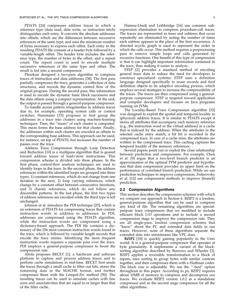
6.2 Compression Rate

Fig. 2 depicts the geometric-mean compression rates of sixalgorithms from the literature on our three types of tracesnormalized to VPC4 (higher numbers are better). For eachtrace type, the algorithms are sorted from left to right byincreasing compression rate. The darker section at the


TABLE 2Geometric-Mean Performance of the VPC Algorithms

Fig. 2. Geometric-mean compression rates normalized to VPC4.


TABLE 3Absolute Compression Rates

bottom of each bar indicates the compression rate after thefirst stage. The total bar height represents the overallcompression rate, including the second stage.

VPC4 delivers the best geometric-mean compression rateon each of the three trace types. SBC, the second bestperformer, comes within 0.2 percet of VPC4 on the cache-miss traces but only reaches slightly over half of VPC4’scompression rate on the other two types of traces. It appearsthat the cache-miss traces contain patterns that are equallyexploitable with SBC and VPC4, while the other two typesof traces include important patterns that only VPC4 cantake advantage of. This makes sense as store addressesoften correlate with the previous addresses produced by thesame store. Similarly, load values correlate with thepreviously fetched values of the same load instruction.Since the ministreams expose these correlations, VPC4 canexploit them. Filtering out some of the values, as is done inthe cache-miss traces, breaks many of these correlations andreduces VPC4’s advantage.

SEQUITUR is the next best performer, except on the store-address traces, where PDATS II and MACHE outperform it.This is probably because these two algorithmswere designedfor address traces. SEQUITUR, on the other hand, does notwork well on long strided sequences, which are common insuch traces. MACHE and BZIP2’s compression rates are inthe lower half, but they both outperform PDATS II on theload-value traces.

Looking at the geometric-mean compression rate of thefirst stage only, we see that SEQUITUR is dominant,followed by SBC. Nevertheless, high initial compressionrates do not guarantee good overall performance. In fact,with the exception of MACHE on the load-value traces (andBZIP2, which has no first stage), all algorithms have ahigher ratio of first-stage to overall compression rate thanVPC4. VPC4’s first stage provides less than 10 percent of thecompression rate on all three types of traces (only0.7 percent on the store-address traces). Note that thesecond stage (BZIP2) boosts the compression rate by morethan a factor of two in all cases.

Table 3 shows the absolute compression rate achieved bythe six algorithms on each individual trace. Only the total

compression rates over both stages are listed.Wehighlightedthe highest compression rate for each trace in bold print. Thetable further includes the harmonic, geometric, and arith-metic mean of the compression rates for each trace type.

We see that no algorithm is the best for all traces.However, VPC4 yields the highest compression rate on allload-value traces. This is most likely because many of thevalue predictors VPC4 uses were specifically designed topredict load values. Moreover, VPC4’s predictor configura-tion was tuned using one of the load-value traces (gcc).

On the cache-miss traces, SBC outperforms all otheralgorithms on six traces, SEQUITUR on two traces, andVPC4 on 10 traces. BZIP2 provides the best compressionrate on four traces, even though it is the only compressorthat has no knowledge of our trace format and all the otheralgorithms use BZIP2 in their second stage. On sixtrack,SEQUITUR outperforms VPC4 by a factor of 5.5, which isthe largest such factor we found. The cache-miss trace bzip2is the least compressible trace in our suite. No algorithmcompresses it by more than a factor of 5.8.

On the store-address traces, which are far morecompressible than the other two types of traces, VPC4yields the highest compression rate on 12 traces, SEQUITURand SBC on three traces each, and PDATS II on one trace.VPC4 surpasses the other algorithms by a factor of 9.7 onart, which it compresses by a factor 77,161, the highestcompression rate we observed.

Overall, VPC4 provides the best compression rate ontwo-thirds of our traces and delivers the highest arithmetic,geometric, and harmonic-mean compression rates on thethree types of traces, though SBC comes close on the cache-miss traces.

6.3 Decompression Time

Fig. 3 shows the geometric-mean decompression time of thesix algorithms on our three types of traces normalized toVPC4 (lower numbers are better). For each trace type, thealgorithms are sorted from left to right by decreasingdecompression time. The darker section at the bottom ofeach bar represents the time spent in the first stage. Thelighter top portion of each bar depicts the time spent in the


Fig. 3. Geometric-mean decompression time normalized to VPC4.


TABLE 4Absolute Decompression Time in Seconds

second stage. The total bar height corresponds to the overalldecompression time. Note that, during decompression, thesecond stage is invoked first.

VPC4 provides the fastest mean decompression time onour traces but SBC and SEQUITUR are close seconds. Theyare only 5 to 36 percent slower. The remaining threealgorithms are at least 60 percent slower. SEQUITUR isfaster on the load-value traces than SBC. The situation isreversed on the other two trace types. The majority of thealgorithms that use BZIP2 in their second stage are fasterthan BZIP2 alone.

Looking at the two stages separately,we find that the threefastest decompressors, VPC4, SBC, and SEQUITUR, spendalmost equal amounts of time in the two stages, except on thestore-address traces, where the second stage (BZIP2)accounts for about a third of the total decompression time.MACHE and PDATS II, on the other hand, typically spendmore time in the second stage than in the first.

Table 4 gives the absolute decompression time inseconds of the six algorithms on each individual trace.Only the total decompression time over both stages is listed.We highlighted the shortest decompression time for eachtrace in bold print. The table further includes the harmonic,geometric, and arithmetic mean of the decompression timesfor each trace type.

SEQUITUR, VPC4, and SBC deliver the fastest decom-pression times on all traces. On the store-address traces,SEQUITUR is fastest on eight and VPC4 on 11 traces. On thecache-miss traces, SBC is fastest on eight and VPC4 andSEQUITUR on seven traces each. On average (any of thethree means), VPC4 outperforms SBC, but SEQUITUR hasthe best overall harmonic-mean decompression time. Onthe load-value traces, SBC is fastest on one, SEQUITUR onfive, and VPC4 on eight traces. Again, SEQUITUR outper-forms VPC4 in the harmonic mean.

VPC4 is maximally 68 percent faster than the otheralgorithms on the load-value trace swim. SEQUITUR is125 percent faster than VPC4 on the cache-miss tracesixtrack. In other words, the range from one extreme to theother is relatively narrow, meaning that VPC4’s decom-pression time and that of the fastest other algorithm arefairly close on all traces.

6.4 Compression Time

Fig. 4 shows the geometric-mean compression time of thesix algorithms on our three types of traces normalized toVPC4 (lower numbers are better). Again, the algorithms aresorted from left to right by decreasing time. The darkersection at the bottom of each bar represents the time spentin the first stage and the lighter top portion depicts the timespent in the second stage. The total bar height correspondsto the overall compression time. On the cache-miss traces,SBC’s first stage takes 13.9 and the second stage 2.3 times aslong as VPC4’s total compression time.

VPC4’s geometric-mean compression time is over threetimes shorter than that of the other algorithms weevaluated. This is particularly surprising as VPC4 alsoachieves the highest mean compression rates (Section 6.2).Typically, one would expect longer computation times toresult in higher compression rates, but not the other wayaround. SBC, the otherwise best non-VPC algorithm, takes9.5 to 16.2 times as long as VPC4 to compress the traces. TheSBC authors verified that the current version of theiralgorithm has not been optimized to provide fast compres-sion. SEQUITUR is 3.6 to 7.7 times slower than VPC4.

SEQUITUR’s algorithm is quite asymmetric, i.e., con-structing the grammar (compression) is a much slowerprocess than recursively traversing it (decompression). Theaverage (geometric mean for the three trace types)compression over decompression time ratio for SEQUITURis 8.8 to 17.7. For BZIP2, it is 5.9 to 11.5, for MACHE, 4.0 to8.7, for PDATS II, 3.7 to 10.6, and, for SBC 19.3, to 43.4.VPC4 is the most symmetric of the six algorithms, whichexplains its fast compression speed. It basically performsthe same operations during compression and decompres-sion. The only asymmetry in VPC4 is that, duringcompression, it needs to check each predictor for a match,which makes compression 2.6 to 3.1 times slower thandecompression.

Looking at the time spent in the two stages, we notice astriking difference between SBC and SEQUITUR on the onehand and VPC4 on the other hand. Both SBC andSEQUITUR spend most of the total compression time inthe first stage. In VPC4, the first stage only contributes 18 to22 percent of the compression time, meaning that the


Fig. 4. Geometric-mean compression time normalized to VPC4.


TABLE 5Absolute Compression Time in Seconds

separation of the traces into the four streams happens veryquickly. Only SEQUITUR spends less time in the secondstage than VPC4 (on the cache-miss and the load-valuetraces). All other algorithms (and SEQUITUR on the store-address traces) spend more time in BZIP2 than VPC4 does.This is the result of our efforts to tune VPC4’s first stage toconvert the traces into a very amenable form for the secondstage (see Sections 4.4 and 4.5).

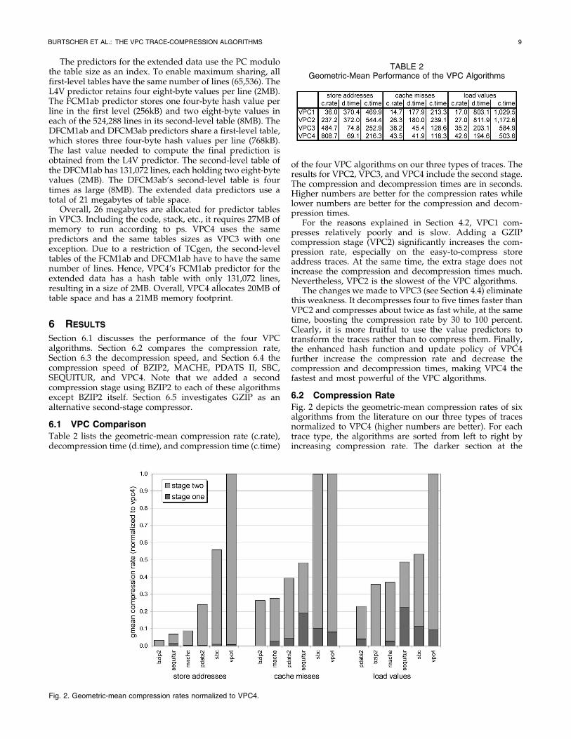
Table 5 lists the absolute compression time in seconds forthe six algorithms on each individual trace. Only the totalcompression time over both stages is included. We high-lighted the shortest compression time for each trace in boldprint. The table also shows the harmonic, geometric, and thearithmeticmean of the compression times for each trace type.

VPC4 compresses 53 of the 55 traces faster than the otherfive algorithms and is also the fastest compressor onaverage. MACHE is 13 percent faster on the mgrid cache-miss trace and PDATS II is 29 percent faster on the vprcache-miss trace. VPC4 compresses the store-address traceart 1,569 percent faster than the other algorithms do.

6.5 Second Stage Compressor

Table 6 shows the geometric-mean compression rate,decompression time, and compression time of SBC andVPC4, the two best-performing trace compressors in theprevious sections, over our three trace types when GZIP isused as the second stage instead of BZIP2. We use GZIPversion 1.3.3 with the “–best” option.

As the results show, VPC4 roughly retains its perfor-mance advantage with the GZIP stage. It is faster anddelivers a higher mean compression rate than SBC excepton the store-address traces, which SBC with GZIP com-presses 1.5 percent more than VPC4 with GZIP. Comparingthe VPC4 results from Table 6 with those from Table 2, wefind that VPC4 compresses better and faster with BZIP2, butdecompresses faster with GZIP.

7 SUMMARY AND CONCLUSIONS

This paper presents the four VPC trace-compression algo-rithms, all of which employ value predictors to compressprogram traces that comprisePCsandother information suchas register values or memory addresses. VPC4, our mostsophisticated approach, converts traces into streams that aremore compressible than the original trace and that can becompressed and decompressed faster. For example, itcompresses SPECcpu2000 traces of store-instruction PCsand effective addresses, traces of thePCs and the addresses ofloads and stores that miss in a simulated cache, and traces ofload instruction PCs and load values better and compressesand decompresses them more quickly than SEQUITUR,BZIP2, MACHE, SBC, and PDATS II. Based on these results,we believe VPC4 to be a good choice for trace databases,where good compression rates are paramount, as well astrace-based research and teaching environments, where afast decompression speed is as essential as a goodcompression rate.

VPC4 features a single-pass linear-time algorithm with afixed memory requirement. It is automatically synthesizedout of a simple user-provided description, making it easy toadapt VPC4 to other trace formats and to tune it.

ACKNOWLEDGMENTS

This work was supported in part by the US National ScienceFoundation under Grant Nos. 0208567 and 0312966. Theauthors would like to thank Metha Jeeradit for hiscontributions to VPC1 and the anonymous reviewers fortheir helpful feedback.

REFERENCES

[1] J. Ahola, “Compressing Address Traces with RECET,” Proc. 2001IEEE Int’l Workshop Workload Characterization, pp. 120-126, Dec.2001.

[2] R. Brown, K. Driesen, D. Eng, L. Hendren, J. Jorgensen, C.Verbrugge, and Q. Wang, “STEP: A Framework for the EfficientEncoding of General Trace Data,” Proc. Workshop Program Analysisfor Software Tools and Eng., pp. 27-34, Nov. 2002.

[3] M. Burrows and D.J. Wheeler, “A Block-Sorting Lossless DataCompression Algorithm,” Digital SRC Research Report 124, May1994.

[4] M. Burtscher, “VPC3: A Fast and Effective Trace-CompressionAlgorithm,” Proc. Joint Int’l Conf. Measurement and Modeling ofComputer Systems, pp. 167-176, June 2004.

[5] M. Burtscher and M. Jeeradit, “Compressing Extended ProgramTraces Using Value Predictors,” Proc. Int’l Conf. Parallel Architec-tures and Compilation Techniques, pp. 159-169, Sept. 2003.

[6] M. Burtscher and N.B. Sam, “Automatic Generation of High-Performance Trace Compressors,” Proc. 2005 Int’l Symp. CodeGeneration and Optimization, pp. 229-240, Mar. 2005.

[7] M. Burtscher and B.G. Zorn, “Exploring Last n Value Prediction,”Proc. Int’l Conf. Parallel Architectures and Compilation Techniques,pp. 66-76, Oct. 1999.

[8] M. Burtscher and B.G. Zorn, “Hybrid Load-Value Predictors,”IEEE Trans. Computers, vol. 51, no. 7, pp. 759-774, July 2002.

[9] I.K. Chen, J.T. Coffey, and T.N. Mudge, “Analysis of BranchPrediction via Data Compression,” Proc. Seventh Int’l Conf.Architectural Support for Programming Languages and OperatingSystems, pp. 128-137, Oct. 1996.

[10] E.N. Elnozahy, “Address Trace Compression through LoopDetection and Reduction,” Proc. Int’l Conf. Measurement andModeling of Computer Systems, pp. 214-215, May 1999.

[11] A. Eustace and A. Srivastava, “ATOM: A Flexible Interface forBuilding High Performance Program Analysis Tools,” WRLTechnical Note TN-44, Digital Western Research Laboratory, PaloAlto, Calif., July 1994.

[12] E. Federovsky, M. Feder, and S. Weiss, “Branch Prediction Basedon Universal Data Compression Algorithms,” Proc. 25th Int’lSymp. Computer Architecture, pp. 62-72, June 1998.

[13] F. Gabbay, “Speculative Execution Based on Value Prediction,”Electrical Eng. Dept. Technical Report #1080, Technion-Israel Inst.of Technology, Nov. 1996.

[14] B. Goeman, H. Vandierendonck, and K. Bosschere, “DifferentialFCM: Increasing Value Prediction Accuracy by Improving TableUsage Efficiency,” Proc. Seventh Int’l Symp. High PerformanceComputer Architecture, pp. 207-216, Jan. 2001.

[15] O. Hammami, “Taking into Account Access Pattern Irregularitywhen Compressing Address Traces,” Proc. Southeastcon, pp. 74-77,Mar. 1995.

[16] A. Hamou-Lhadj and T.C. Lethbridge, “Compression Techniquesto Simplify the Analysis of Large Execution Traces,” Proc. 10thInt’l Workshop Program Comprehension, pp. 159-168, June 2002.

[17] http://sequence.rutgers.edu/sequitur/sequitur.cc, 2005.[18] http://sources.redhat.com/bzip2/, 2005.[19] http://www.cygwin.com/, 2005.[20] http://www.ece.uah.edu/lacasa/sbc/sbc.html, 2005.[21] http://www.gzip.org/, 2005.[22] http://www.spec.org/osg/cpu2000/, 2005.[23] E.E. Johnson, “PDATS II: Improved Compression of Address

Traces,” Proc. Int’l Performance, Computing, and Comm. Conf., pp. 72-78, Feb. 1999.


TABLE 6Geometric-Mean Performance of SBC and VPC4 with GZIP

[24] E.E. Johnson and J. Ha, “PDATS: Lossless Address TraceCompression for Reducing File Size and Access Time,” Proc. IEEEInt’l Phoenix Conf. Computers and Comm., pp. 213-219, Apr. 1994.

[25] E.E. Johnson, J. Ha, and M.B. Zaidi, “Lossless Trace Compres-sion,” IEEE Trans. Computers, vol. 50, no. 2, pp. 158-173, Feb. 2001.

[26] R.E. Kessler, E.J. McLellan, and D.A. Webb, “The Alpha 21264Microprocessor Architecture,” Proc. Int’l Conf. Computer Design,pp. 90-95, Oct. 1998.

[27] D.E. Knuth, “Dynamic Huffman Coding,” J. Algorithms, vol. 6,pp. 163-180, 1985.

[28] J.R. Larus, “Abstract Execution: A Technique for EfficientlyTracing Programs,” Software-Practice and Experience, vol. 20,no. 12, pp. 1241-1258, Dec. 1990.

[29] J.R. Larus, “Whole Program Paths,” Proc. Conf. ProgrammingLanguage Design and Implementation, pp. 259-269, May 1999.

[30] M.H. Lipasti and J.P. Shen, “Exceeding the Dataflow Limit viaValue Prediction,” Proc. 29th Int’l Symp. Microarchitecture, pp. 226-237, Dec. 1996.

[31] M.H. Lipasti, C.B. Wilkerson, and J.P. Shen, “Value Locality andLoad Value Prediction,” Proc. Seventh Int’l Conf. ArchitecturalSupport for Programming Languages and Operating Systems, pp. 138-147, Oct. 1996.

[32] Y. Luo and L.K. John, “Locality-Based Online Trace Compres-sion,” IEEE Trans. Computers, vol. 53, no. 6, pp. 723-731, June 2004.

[33] A. Milenkovic and M. Milenkovic, “Stream-Based Trace Compres-sion,” Computer Architecture Letters, vol. 2, Sept. 2003.

[34] A. Milenkovic and M. Milenkovic, “Exploiting Streams inInstruction and Data Address Trace Compression,” Proc. SixthAnn. Workshop Workload Characterization, pp. 99-107, Oct. 2003.

[35] C.G. Nevill-Manning and I.H. Witten, “Linear-Time, IncrementalHierarchy Interference for Compression,” Proc. Data CompressionConf., pp. 3-11, Mar. 1997.

[36] C.G. Nevill-Manning and I.H. Witten, “Identifying HierarchicalStructure in Sequences: A Linear-Time Algorithm,” J. ArtificialIntelligence Research, vol. 7, pp. 67-82, Sept. 1997.

[37] C.G. Nevill-Manning and I.H. Witten, “Compression and Ex-planation Using Hierarchical Grammars,” The Computer J., vol. 40,pp. 103-116, 1997.

[38] A.R. Pleszkun, “Techniques for Compressing Program AddressTraces,” Proc. 27th Ann. IEEE/ACM Int’l Symp. Microarchitecture,pp. 32-40, Nov. 1994.

[39] G. Reinman and B. Calder, “Predictive Techniques for AggressiveLoad Speculation,” Proc. 31st Int’l Symp. Microarchitecture, pp. 127-137, Dec. 1998.

[40] B. Rychlik, J.W. Faistl, B.P. Krug, and J.P. Shen, “Efficacy andPerformance Impact of Value Prediction,” Proc. Int’l Conf. ParallelArchitectures and Compilation Techniques, pp. 148-154, Oct. 1998.

[41] A.D. Samples, “Mache: No-Loss Trace Compaction,” Proc. Int’lConf. Measurement and Modeling of Computer Systems, vol. 17, no. 1,pp. 89-97, Apr. 1989.

[42] Y. Sazeides and J.E. Smith, “Implementations of Context BasedValue Predictors,” Technical Report ECE-97-8, Univ. of Wiscon-sin-Madison, Dec. 1997.

[43] Y. Sazeides and J.E. Smith, “The Predictability of Data Values,”Proc. 30th Int’l Symp. Microarchitecture, pp. 248-258, Dec. 1997.

[44] A. Srivastava and A. Eustace, “ATOM: A System for BuildingCustomized Program Analysis Tools,” Proc. Conf. ProgrammingLanguage Design and Implementation, pp. 196-205, June 1994.

[45] D. Tullsen and J. Seng, “Storageless Value Prediction Using PriorRegister Values,” Proc. 26th Int’l Symp. Computer Architecture,pp. 270-279, May 1999.

[46] J.S. Vitter, “Design and Analysis of Dynamic Huffman Codes,”J. ACM, vol. 34, no. 4, pp. 825-845, Oct. 1987.

[47] K. Wang and M. Franklin, “Highly Accurate Data ValuePrediction Using Hybrid Predictors,” Proc. 30th Int’l Symp.Microarchitecture, pp. 281-290, Dec. 1997.

[48] T.A. Welch, “A Technique for High-Performance Data Compres-sion,” Computer, pp. 8-19, June 1984.

[49] Y. Zhang and R. Gupta, “Timestamped Whole Program PathRepresentation and Its Applications,” Proc. Conf. ProgrammingLanguage Design and Implementation, pp. 180-190, June 2001.

[50] J. Ziv and A. Lempel, “A Universal Algorithm for DataCompression,” IEEE Trans. Information Theory, vol. 23, no. 3,pp. 337-343, May 1977.

Martin Burtscher received the combined BS/MS degree in computer science from the SwissFederal Institute of Technology (ETH) Zurich in1996 and the PhD degree in computer sciencefrom the University of Colorado at Boulder in2000. He is an assistant professor in the Schoolof Electrical and Computer Engineering atCornell University, where he leads the High-Performance Microprocessor Systems Group.His current research focuses on hardware-

based prefetching, trace compression, self-tuning hardware, MPIlibraries, value-based compiler optimizations, energy and complexityefficient architectures, and brain injury simulation. He is a member of theIEEE, the IEEE Computer Society, and the ACM.

Ilya Ganusov received the Electronics Engineerdegree from Ivanovo State Power University,Russian Federation, in 2001 and the MS degreein electrical and computer engineering fromCornell University in 2005. He is currently aPhD candidate in electrical and computerengineering at Cornell University. His researchinterests focus on high-performance micropro-cessor architectures, spanning prediction andspeculation, prefetching techniques, multi-

threading, and compiler technology. He is a student member of theIEEE and the ACM.

Sandra J. Jackson received the BS degree incomputer science from Cornell University in1999. She is an MS/PhD student in electricaland computer engineering at Cornell University.Her research interests include genetic algo-rithms, value prediction, and asynchronous VLSI.

Jian Ke received the BS degree in physics fromthe University of Science and Technology ofChina in 1995. He is a PhD candidate in theSchool of Electrical and Computer Engineeringat Cornell University. His research interests arein parallel and distributed computing systemsand high-performance computer architectures.

Paruj Ratanaworabhan received the BEng andMEng degrees in electrical engineering fromKasetsart University and Cornell University,respectively. He joined the PhD program incomputer engineering at the Georgia Institute ofTechnology in the fall of 2002. His researchfocus then was on microprocessor verification.After a year at Georgia Tech, he returned toCornell University. Since then, his researchfocus has been on value prediction and its

applications to compiler optimization.

Nana B. Sam received the BSc degree inelectrical and electronic engineering from theUniversity of Science and Technology, Ghana,in 2000 and the MS degree in electrical andcomputer engineering from Cornell University in2003. She is a PhD student in electrical andcomputer engineering at Cornell University andis currently an intern at the IBM T.J. WatsonResearch Center. Her research interests includeenergy-aware microprocessor design and math-

ematical modeling for design complexity analyses. She is a studentmember of the IEEE and the IEEE Computer Society.


Documents

IEEE TRANSACTIONS ON COMPUTERS, VOL.54, …cs.txstate.edu/~burtscher/papers/tc05.pdfThe VPC Trace-Compression Algorithms Martin Burtscher, Member, IEEE, Ilya Ganusov, Student Member,