Embed Size (px)
Citation preview
IEEE Std C37.114™-2004
C37.114TM
IEEE Guide for Determining FaultLocation on AC Transmission andDistribution Lines
3 Park Avenue, New York, NY 10016-5997, USA
IEEE Power Engineering Society
Sponsored by thePower System Relaying Committee
8 June 2005
Print: SH95314PDF: SS95314

The Institute of Electrical and Electronics Engineers, Inc.3 Park Avenue, New York, NY 10016-5997, USA
Copyright © 2005 by the Institute of Electrical and Electronics Engineers, Inc.All rights reserved. Published 8 June 2005. Printed in the United States of America.
IEEE is a registered trademark in the U.S. Patent & Trademark Office, owned by the Institute of Electrical and ElectronicsEngineers, Incorporated.
Print: ISBN 0-7381-4653-6 SH95314PDF: ISBN 0-7381-4654-4 SS95314
No part of this publication may be reproduced in any form, in an electronic retrieval system or otherwise, without the priorwritten permission of the publisher.
IEEE Std C37.114™-2004
IEEE Guide for Determining Fault Location on AC Transmission and Distribution Lines
Sponsor
Power System Relaying Committeeof theIEEE Power Engineering Society
Approved 8 December 2004
IEEE-SA Standards Board
Abstract: Electrical faults on transmission and distribution lines are detected and isolated bysystem protective devices. Once the fault has been cleared, outage times can be reduced if thelocation of the fault can be determined more quickly. This guide outlines the techniques andapplication considerations for determining the location of a fault on ac transmission and distributionlines. The document reviews traditional approaches and the primary measurement techniques usedin modern devices: one-terminal and two-terminal impedance-based methods and traveling wavemethods. Application considerations include: two- and three-terminal lines, series-compensatedlines, parallel lines, untransposed lines, underground cables, fault resistance effects, and otherpower system conditions, including those unique to distribution systems.Keywords: fault location, relays, system protection, traveling waves
IEEE Standards documents are developed within the IEEE Societies and the Standards Coordinating Committees of theIEEE Standards Association (IEEE-SA) Standards Board. The IEEE develops its standards through a consensusdevelopment process, approved by the American National Standards Institute, which brings together volunteersrepresenting varied viewpoints and interests to achieve the final product. Volunteers are not necessarily members of theInstitute and serve without compensation. While the IEEE administers the process and establishes rules to promote fairnessin the consensus development process, the IEEE does not independently evaluate, test, or verify the accuracy of any of theinformation contained in its standards.
Use of an IEEE Standard is wholly voluntary. The IEEE disclaims liability for any personal injury, property or otherdamage, of any nature whatsoever, whether special, indirect, consequential, or compensatory, directly or indirectly resultingfrom the publication, use of, or reliance upon this, or any other IEEE Standard document.
The IEEE does not warrant or represent the accuracy or content of the material contained herein, and expressly disclaimsany express or implied warranty, including any implied warranty of merchantability or fitness for a specific purpose, or thatthe use of the material contained herein is free from patent infringement. IEEE Standards documents are supplied “AS IS.”
The existence of an IEEE Standard does not imply that there are no other ways to produce, test, measure, purchase, market,or provide other goods and services related to the scope of the IEEE Standard. Furthermore, the viewpoint expressed at thetime a standard is approved and issued is subject to change brought about through developments in the state of the art andcomments received from users of the standard. Every IEEE Standard is subjected to review at least every five years forrevision or reaffirmation. When a document is more than five years old and has not been reaffirmed, it is reasonable toconclude that its contents, although still of some value, do not wholly reflect the present state of the art. Users are cautionedto check to determine that they have the latest edition of any IEEE Standard.
In publishing and making this document available, the IEEE is not suggesting or rendering professional or other servicesfor, or on behalf of, any person or entity. Nor is the IEEE undertaking to perform any duty owed by any other person orentity to another. Any person utilizing this, and any other IEEE Standards document, should rely upon the advice of acompetent professional in determining the exercise of reasonable care in any given circumstances.
Interpretations: Occasionally questions may arise regarding the meaning of portions of standards as they relate to specificapplications. When the need for interpretations is brought to the attention of IEEE, the Institute will initiate action to prepareappropriate responses. Since IEEE Standards represent a consensus of concerned interests, it is important to ensure that anyinterpretation has also received the concurrence of a balance of interests. For this reason, IEEE and the members of itssocieties and Standards Coordinating Committees are not able to provide an instant response to interpretation requests exceptin those cases where the matter has previously received formal consideration. At lectures, symposia, seminars, or educationalcourses, an individual presenting information on IEEE standards shall make it clear that his or her views should be consideredthe personal views of that individual rather than the formal position, explanation, or interpretation of the IEEE.
Comments for revision of IEEE Standards are welcome from any interested party, regardless of membership affiliation withIEEE. Suggestions for changes in documents should be in the form of a proposed change of text, together with appropriatesupporting comments. Comments on standards and requests for interpretations should be addressed to:
Secretary, IEEE-SA Standards Board
445 Hoes Lane
Piscataway, NJ 08854
USA
Authorization to photocopy portions of any individual standard for internal or personal use is granted by the Institute ofElectrical and Electronics Engineers, Inc., provided that the appropriate fee is paid to Copyright Clearance Center. Toarrange for payment of licensing fee, please contact Copyright Clearance Center, Customer Service, 222 Rosewood Drive,Danvers, MA 01923 USA; +1 978 750 8400. Permission to photocopy portions of any individual standard for educationalclassroom use can also be obtained through the Copyright Clearance Center.
NOTE−Attention is called to the possibility that implementation of this standard may require use of subjectmatter covered by patent rights. By publication of this standard, no position is taken with respect to the exist-ence or validity of any patent rights in connection therewith. The IEEE shall not be responsible for identifyingpatents for which a license may be required by an IEEE standard or for conducting inquiries into the legal valid-ity or scope of those patents that are brought to its attention.
iiiCopyright © 2005 IEEE. All rights reserved.
Introduction
This guide shall outline the techniques and application considerations for determining the location of a faulton AC transmission and distribution lines. We shall review traditional approaches and the primarymeasurement techniques used in modern devices: one-terminal and two-terminal impedance-based methodsand traveling wave methods. Application considerations include: two- and three-terminal lines, series-compensated lines, parallel lines, untransposed lines, underground cables, fault resistance effects, and otherpower system conditions, including those unique to distribution systems.
Notice to users
Errata
Errata, if any, for this and all other standards can be accessed at the following URL: http://standards.ieee.org/reading/ieee/updates/errata/index.html. Users are encouraged to check this URL forerrata periodically.
Interpretations
Current interpretations can be accessed at the following URL: http://standards.ieee.org/reading/ieee/interp/index.html.
Patents
Attention is called to the possibility that implementation of this standard may require use of subject mattercovered by patent rights. By publication of this standard, no position is taken with respect to the existence orvalidity of any patent rights in connection therewith. The IEEE shall not be responsible for identifyingpatents or patent applications for which a license may be required to implement an IEEE standard or forconducting inquiries into the legal validity or scope of those patents that are brought to its attention.
This introduction in not part of IEEE Std C37.114-2004, IEEE Guide for Determining Fault Location on ACTransmission and Distribution Lines.

ivCopyright © 2005 IEEE. All rights reserved.
ParticipantsThe following is a list of participants in the Fault Location Working Group:
Karl Zimmerman, ChairD. J. Novosel, Vice-Chair
The following members of the individual balloting committee voted on this standard. Balloters may havevoted for approval, disapproval, or abstention.
When the IEEE-SA Standards Board approved this standard on 8 December 2004, it had the followingmembership:
Don Wright, ChairSteve M. Mills, Vice ChairJudith Gorman, Secretary
*Member Emeritus
Also included are the following nonvoting IEEE-SA Standards Board liaisons:
Satish K. Aggarwal, NRC RepresentativeRichard DeBlasio, DOE Representative
Alan Cookson, NIST Representative
Jennie SteinhagenIEEE Standards Project Editor
G. E. AlexanderA. ApostolovL. BudlerP. T. CarrollJ. DelareeP. Gale
B. JacksonH. JacobiM. KezunovicW. G. LoweR. MarttilaM. J. McDonaldM. S. Sachdev
T. SeegersH. M. ShuhT. S. SidhuD. TziouvarasJ. E. WaldronR. Young
William AckermanSteve AlexandersonGabriel BenmouyalKenneth BirtStuart BorlaseStuart BoucheyDaniel BrosnanGustavo BrunelloCarlos CastroJohn W. Chadwick, Jr.Stephen ConradRobert CopyakJames R CornelisonLuis CoronadoRonald DauberDouglas DawsonSantpal DhillonGuru Dutt DhingraRandall DotsonPaul Drum
Ahmed ElneweihiGary EngmannKenneth FoderoAnthony GiulianteManuel GonzalezAjit GwalRoger HeddingJames D. Huddleston IIIDavid JacksonJoseph L. KoepfingerDavid KrauseGregory LuriKeith MalmedalJesus MartinezThomas McCaffreyMichael McDonaldJeff McElrayMark McGranaghanGary MichelDean MillerBill Moncrief
Anthony NapikoskiCharles RogersJames RuggieriMohindar SachdevTony SeegersTom ShortH. Jin SimMark SimonHarinderpal SinghKevin StephanJames StonerGlenn SwiftRick TaylorJohn TengdinEric UdrenGerald VaughnCharles WagnerPhilip WinstonRay YoungKarl Zimmerman
Chuck AdamsStephen BergerMark D. BowmanJoseph A. BruderBob DavisRoberto de Marca BoissonJulian Forster*Arnold M. GreenspanMark S. Halpin
Raymond HapemanRichard J. HollemanRichard H. HulettLowell G. JohnsonJoseph L. Koepfinger*Hermann KochThomas J. McGean
Daleep C. MohlaPaul NikolichT. W. OlsenRonald C. PetersenGary S. RobinsonFrank StoneMalcolm V. ThadenDoug ToppingJoe D. Watson
Contents 1. Overview .................................................................................................................................................... 1
1.1 Scope ................................................................................................................................................... 1 1.2 How to determine line parameters ....................................................................................................... 2
2. References .................................................................................................................................................. 3
3. Definitions, acronyms, and abbreviations .................................................................................................. 3
3.1 Definitions ........................................................................................................................................... 3 3.2 Acronyms and abbreviations ............................................................................................................... 4
4. One-ended impedance-based measurement techniques.............................................................................. 4
4.1 Implementation: data and equipment required .................................................................................... 5 4.2 System parameters and main sources of error: fault resistance and load............................................. 6 4.3 Algorithms........................................................................................................................................... 8
5. Two-terminal data methods ...................................................................................................................... 10
5.1 Implementation: data and equipment required .................................................................................. 10 5.2 System parameters ............................................................................................................................. 11 5.3 Algorithms......................................................................................................................................... 11
6. Other fault location applications............................................................................................................... 12
6.1 Three-terminal lines........................................................................................................................... 12 6.2 Series-compensated lines................................................................................................................... 12 6.3 Parallel lines ...................................................................................................................................... 15 6.4 Distribution system faults .................................................................................................................. 16 6.5 Locating faults on underground cables, paralleled cable circuits ...................................................... 18 6.6 Automatic reclosing effects on fault locating .................................................................................... 20 6.7 Effect of tapped load.......................................................................................................................... 20 6.8 Phase selection, fault identification, sequential faults ....................................................................... 21 6.9 Long lines and reactor and capacitor installations ............................................................................. 21 6.10 Short duration faults ........................................................................................................................ 21 6.11 Effect of untransposed lines on accuracy of line parameters ........................................................... 22 6.12 Comparison of one-terminal and two-terminal impedance-based methods..................................... 23
7. Traveling wave techniques ....................................................................................................................... 26
7.1 Data and equipment required............................................................................................................. 27 7.2 Accuracy limitations.......................................................................................................................... 27 7.3 Traveling wave methods.................................................................................................................... 28
8. Other techniques....................................................................................................................................... 29
8.1 Methods using synchronized phasors ................................................................................................ 29 8.2 Methods requiring time-tagging of the events ................................................................................... 29
9. Conclusion................................................................................................................................................ 29
Annex A (informative) Bibliography ........................................................................................................... 31
Annex B (informative) Additional information on series-compensated lines .............................................. 34

1 Copyright © 2005 IEEE. All rights reserved.
IEEE Guide for Determining Fault Location on AC Transmission and Distribution Lines
1. Overview
1.1 Scope
This guide outlines the techniques and application considerations for determining the location of a fault on ac transmission and distribution lines. This document reviews traditional approaches and the primary measurement techniques used in modern devices: one-terminal and two-terminal impedance-based methods and traveling wave methods. Application considerations include: two- and three-terminal lines, series-compensated lines, parallel lines, untransposed lines, underground cables, fault resistance effects, and other power system conditions, including those unique to distribution systems.
This guide discusses various approaches to determine fault location, with emphasis on automatic methods performed by microprocessor devices. The following are some techniques used to determine fault location:
a) Microprocessor devices
b) Short-circuit analysis software
c) Customer calls (distribution)
d) Line inspection
A device capable of determining the physical fault location has different requirements than a fault detection device.
a) The speed to determine fault location is for human users (seconds or minutes), while relays usually need to detect fault within 10 ms to 50 ms. Consequently, additional information and more demanding and slower numerical techniques become available.
b) A best fault data window can be selected to reduce errors.
c) Communications enable transmitting data to a remote site using low-speed data communications or supervisory control and data acquisition (SCADA).
d) More accurate phasor calculations can be achieved by using digital filtering of the voltage and current samples that would introduce an unacceptable delay for the relaying applications.
e) High accuracy is needed for efficient dispatch of repair crews. Unlike protective relays, which need to detect whether faults are in the zones established by ct locations, pilot channels, and reach coordination, fault location data must be very accurate to save the time and reduce the expenses of the crews searching in bad weather and/or over rough terrain.
IEEE Std C37.114-2004 IEEE Guide for Determining Fault Location on AC Transmission and Distribution Lines
In this guide, the following are examined:
⎯ Data and equipment required
⎯ Common algorithms
⎯ Accuracy limitations of one-ended and two-ended impedance-based fault location methods
⎯ Traveling wave methods and other methods
⎯ Issues regarding distribution systems and underground cables
1.2
1.2.1
1.2.2
How to determine line parameters
Line parameters for impedance estimation
Accurate fault location based upon impedance estimation will depend on the accuracy of calculated transmission impedances. The common method of calculation is based on equations developed by J.R. Carson, et al., and published in 1926 [B1]. There are many good textbooks devoted to the topic of power system analysis that will show the development of Carson’s equations used for determining the line impedances. It is not necessary to show the development of these equations here. Relay engineers have used the equations for many years to model power systems for performing short circuit studies. A typical short circuit computer program would utilize short or medium length line impedances derived from calculations based upon the assumption of fully transposed lines over a homogeneous right-of-way. The only significant details added to the model are the effects of zero-sequence mutual coupling between parallel sections of lines. The results obtained from these impedance models for determining relay coordination and performing postmortem analysis are very good. The question that remains is whether these calculated impedances are sufficient to obtain the desired level of accuracy in the location of faults. Accuracy to within 1% of error has been claimed for the calculated impedances (Eriksson, et al. [B2]).
Another method of determining the line impedance parameters involves the direct measurement of the open circuit, and short circuit voltages and currents. The accuracy is about the same as calculations based on Carson’s equations. This method would require special equipment to set up the tests.
A third method involves the estimation of the line parameters through the solution of two-port equations based on synchronous phasor measurements obtained from direct measurements from a digital relay or a fault recorder. The use of controlled tests to obtain the data and using the higher sampling rate of a digital recorder can result in impedance parameters with a high accuracy. It should be noted that all three techniques rely on an accurate value for the length of the line.
It is suggested that the calculations for most lines can still be made using Carson’s equations. These parameters can then be verified using the synchronous phasors of method three or by experience from the calculation of the locations from faults with verifiable locations. In spite of the accuracy of the line impedance parameters, the accuracy of fault location will be dependent upon the location technique employed, the sampling rate of the data collected, and the presence of unknown variables, most notably the amount of fault resistance.
Line parameter errors introduced on lines without transpositions are described in Annex A.
Parameters required for the traveling wave fault locating
When a current-based traveling wave fault locator is commissioned, the remote units are programmed with the substation and line name, sensitivity, and default sampling settings. No specific line parameters (impedances, etc.) are required for the remote units. The host personal computer, on command, can receive the data from each of the remote units. Once the PC has the data files, the information is analyzed and the line length can be determined. The only inputs required to analyze fault data with the traveling wave fault locator are line length and wave velocity. The individual line length can be determined by energizing the
2 Copyright © 2005 IEEE. All rights reserved.
IEEE Std C37.114-2004 IEEE Guide for Determining Fault Location on AC Transmission and Distribution Lines
line. The procedure is to energize the line in a radial fashion and then measure the time the reflected wave takes to return to the source. The known line length is compared with the length determined by the timing of the reflected wave. This method may not always give accurate results due to the effects of pre-insertion resistors and the closing point on the voltage sine wave. It is not always necessary to rely solely on this method because the line length calibration can also be determined from evaluation of any faults occurring on adjacent line sections.
2.
3.
3.1
References
The following referenced documents are indispensable for the application of this standard. For dated references, only the edition cited applies. For undated references, the latest edition of the referenced document (including any amendments or corrigenda) applies.
IEEE Std C37.2™, IEEE Standard Electrical Power System Device Function Numbers and Contact Designations.1,2
IEEE Std C37.90™, IEEE Standard for Relays and Relay Systems Associated with Electric Power Apparatus.
Definitions, acronyms, and abbreviations
Definitions
For the purposes of this guide, the following terms and definitions apply. The Authoritative Dictionary of IEEE Standards Terms, [B3]3, should be referenced for terms not defined in this clause.
3.1.1 dc thumping: A procedure of applying dc voltage pulses to an underground cable with the intent of locating a cable irregularity with a listening device.
3.1.2 digital recorder: A device that can perform analog-to-digital conversions and store the information in digital form for later retrieval.
3.1.3 distributed intelligence: Gathering data from many different devices for analysis and decision making in a central device.
3.1.4 evolving fault: A fault where the phases involved change over time. For example, a phase-to-ground fault becomes a phase-to-phase-to-ground fault.
3.1.5 fault location error: Percentage error in fault location estimate based on the total line length: e (error) = (instrument reading – exact distance to the fault) / total line length.
3.1.6 GPS time synchronization: A method of using a time signal from the global positioning system (GPS) satellite system for time-synchronizing equipment.
3.1.7 homogeneous line: A transmission line where impedance is distributed uniformly on the whole length.
3.1.8 homogeneous system: A transmission system where the local and remote source impedances have the same system angle as the line impedance.
3.1.9 nomograph: A graph that plots measured fault location versus actual fault location by compensating for known system errors.
1 The IEEE standards or products referred to in this clause are trademarks of the Institute of Electrical and Electronics Engineers, Inc. 2 IEEE publications are available from the Institute of Electrical and Electronics Engineers, Inc., 445 Hoes Lane, Piscataway, NJ 08854, USA (http://standards.ieee.org/). 3 The numbers in brackets correspond to those of the bibliography in Annex A.
3 Copyright © 2005 IEEE. All rights reserved.
IEEE Std C37.114-2004 IEEE Guide for Determining Fault Location on AC Transmission and Distribution Lines
3.1.10 Peterson’s coil: A tunable reactor used for impedance grounding a distribution or transmission system that is usually tuned to the resonance of the system.
3.1.11 pre-insertion resistor: A resistor that is inserted in parallel with each set of breaker contacts during the closing stroke of the breaker.
3.1.12 series-compensated line: A transmission line with series capacitors.
3.1.13 superposition current: The summation current at any point in a linear network that results from the voltages applied at various points in the network.
3.1.14 synchronous phasor: Phasor measurements taken at some point in time that can be referenced to measurements from other locations taken at the same point in time.
3.1.15 time code stamping: Associating an accurate time with a particular event.
3.1.16 traveling wave: The resulting wave when the electric variation in a circuit takes the form of translation of energy along a conductor, such energy being always equally divided between current and potential forms.
3.2
4.
Table 1
Acronyms and abbreviations
CVT capacitive voltage transformers
DMS distribution management system
HMI human-machine interface
MOV metal oxide varistors
SCADA supervisory control and data acquisition
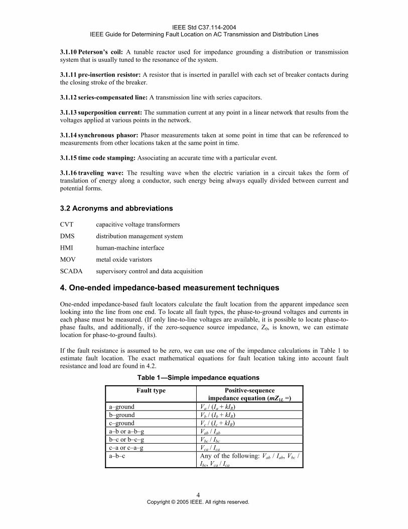
One-ended impedance-based measurement techniques
One-ended impedance-based fault locators calculate the fault location from the apparent impedance seen looking into the line from one end. To locate all fault types, the phase-to-ground voltages and currents in each phase must be measured. (If only line-to-line voltages are available, it is possible to locate phase-to-phase faults, and additionally, if the zero-sequence source impedance, Z0, is known, we can estimate location for phase-to-ground faults).
If the fault resistance is assumed to be zero, we can use one of the impedance calculations in Table 1 to estimate fault location. The exact mathematical equations for fault location taking into account fault resistance and load are found in 4.2.
—Simple impedance equations
Fault type Positive-sequence impedance equation (mZ1L =)
a–ground Va / (Ia + kIR) b–ground Vb / (Ib + kIR) c–ground Vc / (Ic + kIR) a–b or a–b–g Vab / Iab b–c or b–c–g Vbc / Ibc c–a or c–a–g Vca / Ica a–b–c Any of the following: Vab / Iab, Vbc /
Ibc, Vca / Ica
4 Copyright © 2005 IEEE. All rights reserved.
IEEE Std C37.114-2004 IEEE Guide for Determining Fault Location on AC Transmission and Distribution Lines
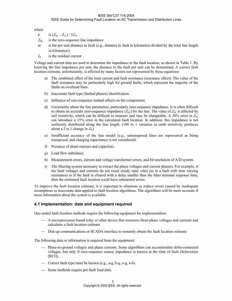
where k is (Z0L – Z1L) / 3Z1L Z0L is the zero-sequence line impedance m is the per unit distance to fault (e.g., distance to fault in kilometers divided by the total line length
in kilometers) IR is the residual current
Voltage and current data are used to determine the impedance to the fault location, as shown in Table 1. By knowing the line impedance per unit, the distance to the fault per unit can be determined. A correct fault location estimate, unfortunately, is affected by many factors not represented by these equations:
a) The combined effect of the load current and fault resistance (reactance effect). The value of the fault resistance may be particularly high for ground faults, which represent the majority of the faults on overhead lines.
b) Inaccurate fault type (faulted phases) identification.
c) Influence of zero-sequence mutual effects on the components.
d) Uncertainty about the line parameters, particularly zero-sequence impedance. It is often difficult to obtain an accurate zero-sequence impedance (Z0L) for the line. The value of Z0L is affected by soil resistivity, which can be difficult to measure and may be changeable. A 20% error in Z0L can introduce a 15% error in the calculated fault location. In addition, this impedance is not uniformly distributed along the line length. (100 to 1 variation in earth resistivity produces about a 2 to 1 change in Z0.)
e) Insufficient accuracy of the line model (e.g., untransposed lines are represented as being transposed, and charging capacitance is not considered).
f) Presence of shunt reactors and capacitors.
g) Load flow unbalance.
h) Measurement errors, current and voltage transformer errors, and bit resolution of A/D system.
i) The filtering system necessary to extract the phase voltages and current phasors. For example, if the fault voltages and currents do not reach steady state value (as in a fault with time varying resistance) or if the fault is cleared with a delay smaller than the filter nominal response time, then the estimated fault location could have substantial errors.
To improve the fault location estimate, it is important to eliminate or reduce errors caused by inadequate assumptions or inaccurate data applied to fault location algorithms. The algorithms will be more accurate if more information about the system is available.
4.1 Implementation: data and equipment required
One-ended fault location methods require the following equipment for implementation:
⎯ A microprocessor-based relay or other device that measures three-phase voltages and currents and calculates a fault location estimate
⎯ Dial-up communications or SCADA interface to remotely obtain the fault location estimate
The following data or information is required from the equipment:
⎯ Phase-to-ground voltages and phase currents. Some algorithms can accommodate delta-connected voltages, but only if zero-sequence source impedance is known at the time of fault (Schweitzer [B15]).
⎯ Correct fault type must be known (e.g., a-g, b-g, c-g, a-b).
⎯ Some methods require pre-fault load data.
5 Copyright © 2005 IEEE. All rights reserved.
IEEE Std C37.114-2004 IEEE Guide for Determining Fault Location on AC Transmission and Distribution Lines
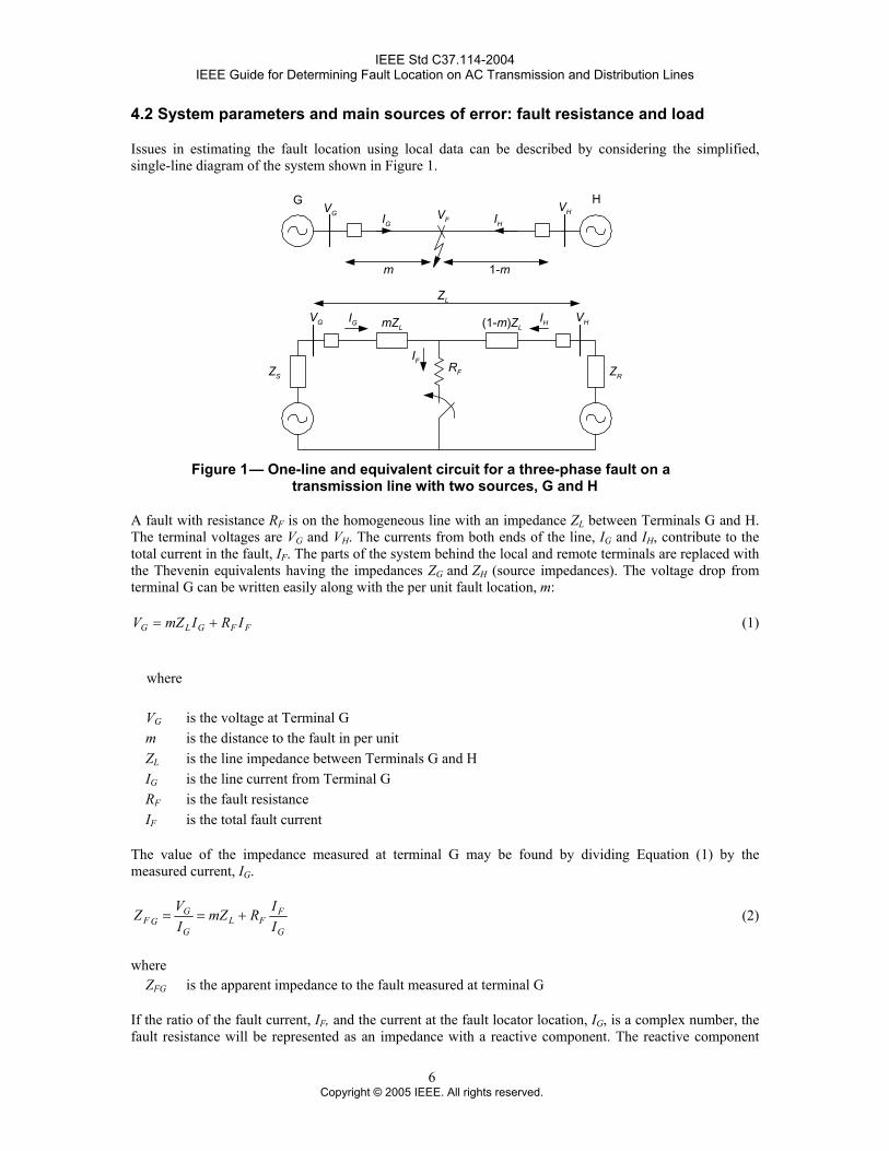
4.2 System parameters and main sources of error: fault resistance and load
Issues in estimating the fault location using local data can be described by considering the simplified, single-line diagram of the system shown in Figure 1.
G HVHVFVG IG IH
m 1-m
RF
IF
ZL
mZL (1-m)ZLIG IH
ZS ZR
VG VH
Figure 1 — One-line and equivalent circuit for a three-phase fault on a
transmission line with two sources, G and H
A fault with resistance RF is on the homogeneous line with an impedance ZL between Terminals G and H. The terminal voltages are VG and VH. The currents from both ends of the line, IG and IH, contribute to the total current in the fault, IF. The parts of the system behind the local and remote terminals are replaced with the Thevenin equivalents having the impedances ZG and ZH (source impedances). The voltage drop from terminal G can be written easily along with the per unit fault location, m:
FFGLG IRImZV += (1)
where
VG is the voltage at Terminal G m is the distance to the fault in per unit ZL is the line impedance between Terminals G and H IG is the line current from Terminal G RF is the fault resistance IF is the total fault current
The value of the impedance measured at terminal G may be found by dividing Equation (1) by the measured current, IG.
G
FFL
G
GGF I
IRmZIVZ +== (2)
where ZFG is the apparent impedance to the fault measured at terminal G
If the ratio of the fault current, IF, and the current at the fault locator location, IG, is a complex number, the fault resistance will be represented as an impedance with a reactive component. The reactive component
6 Copyright © 2005 IEEE. All rights reserved.
IEEE Std C37.114-2004 IEEE Guide for Determining Fault Location on AC Transmission and Distribution Lines
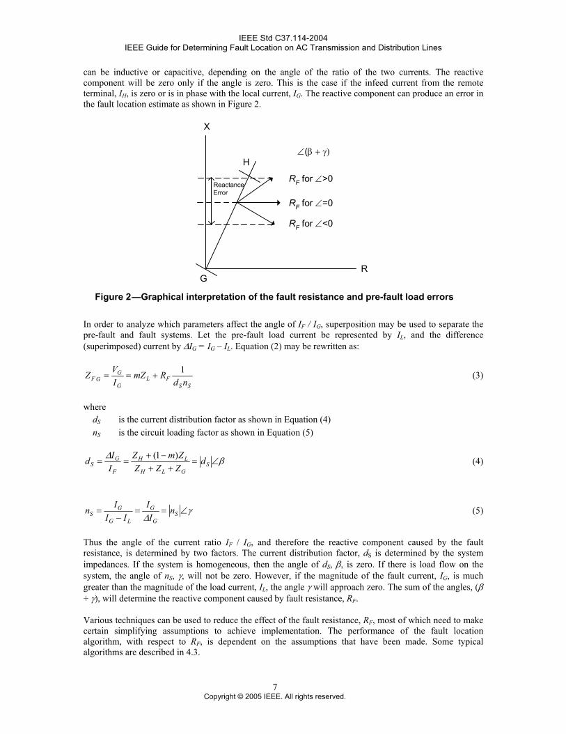
can be inductive or capacitive, depending on the angle of the ratio of the two currents. The reactive component will be zero only if the angle is zero. This is the case if the infeed current from the remote terminal, IH, is zero or is in phase with the local current, IG. The reactive component can produce an error in the fault location estimate as shown in Figure 2.
X
R
H
G
RF for ∠=0
RF for ∠>0
RF for ∠<0
ReactanceError
∠(β + γ)
Figure 2 —Graphical interpretation of the fault resistance and pre-fault load errors
In order to analyze which parameters affect the angle of IF / IG, superposition may be used to separate the pre-fault and fault systems. Let the pre-fault load current be represented by IL, and the difference (superimposed) current by ∆IG = IG – IL. Equation (2) may be rewritten as:
SSFL
G
GGF nd
RmZIVZ 1
+== (3)
where dS is the current distribution factor as shown in Equation (4) nS is the circuit loading factor as shown in Equation (5)
β∆∠=
++−+
== SGLH
LH
F
GS d
ZZZZmZ
IId )1( (4)
γ∆
∠==−
= SG
G
LG
GS n
II
IIIn (5)
Thus the angle of the current ratio IF / IG, and therefore the reactive component caused by the fault resistance, is determined by two factors. The current distribution factor, dS is determined by the system impedances. If the system is homogeneous, then the angle of dS, β, is zero. If there is load flow on the system, the angle of nS, γ, will not be zero. However, if the magnitude of the fault current, IG, is much greater than the magnitude of the load current, IL, the angle γ will approach zero. The sum of the angles, (β + γ), will determine the reactive component caused by fault resistance, RF.
Various techniques can be used to reduce the effect of the fault resistance, RF, most of which need to make certain simplifying assumptions to achieve implementation. The performance of the fault location algorithm, with respect to RF, is dependent on the assumptions that have been made. Some typical algorithms are described in 4.3.
7 Copyright © 2005 IEEE. All rights reserved.
IEEE Std C37.114-2004 IEEE Guide for Determining Fault Location on AC Transmission and Distribution Lines
4.3
4.3.1
Algorithms
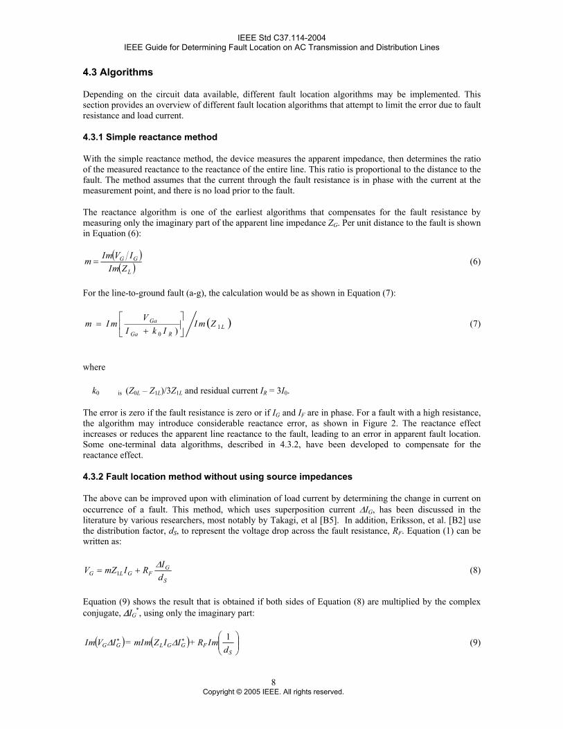
Depending on the circuit data available, different fault location algorithms may be implemented. This section provides an overview of different fault location algorithms that attempt to limit the error due to fault resistance and load current.
Simple reactance method
With the simple reactance method, the device measures the apparent impedance, then determines the ratio of the measured reactance to the reactance of the entire line. This ratio is proportional to the distance to the fault. The method assumes that the current through the fault resistance is in phase with the current at the measurement point, and there is no load prior to the fault.
The reactance algorithm is one of the earliest algorithms that compensates for the fault resistance by measuring only the imaginary part of the apparent line impedance ZG. Per unit distance to the fault is shown in Equation (6):
( )( )L
GG
ZmIIVmIm = (6)
For the line-to-ground fault (a-g), the calculation would be as shown in Equation (7):
( )LRGa
Ga ZmIIkI
VmIm 1
0 ) ⎥⎦
⎤⎢⎣
⎡+
= (7)
where
k0 is (Z0L – Z1L)/3Z1L and residual current IR = 3I0.
The error is zero if the fault resistance is zero or if IG and IF are in phase. For a fault with a high resistance, the algorithm may introduce considerable reactance error, as shown in Figure 2. The reactance effect increases or reduces the apparent line reactance to the fault, leading to an error in apparent fault location. Some one-terminal data algorithms, described in 4.3.2, have been developed to compensate for the reactance effect.
4.3.2 Fault location method without using source impedances
The above can be improved upon with elimination of load current by determining the change in current on occurrence of a fault. This method, which uses superposition current ∆IG, has been discussed in the literature by various researchers, most notably by Takagi, et al [B5]. In addition, Eriksson, et al. [B2] use the distribution factor, dS, to represent the voltage drop across the fault resistance, RF. Equation (1) can be written as:
S
GFGLG d
IRImZV ∆+= 1 (8)
Equation (9) shows the result that is obtained if both sides of Equation (8) are multiplied by the complex conjugate, ∆IG
*, using only the imaginary part:
( ) ( ) ⎟⎟⎠
⎞⎜⎜⎝
⎛
SFGGLGG d
mIR+IIZmmI=IVmI 1** ∆∆ (9)
8 Copyright © 2005 IEEE. All rights reserved.
IEEE Std C37.114-2004 IEEE Guide for Determining Fault Location on AC Transmission and Distribution Lines
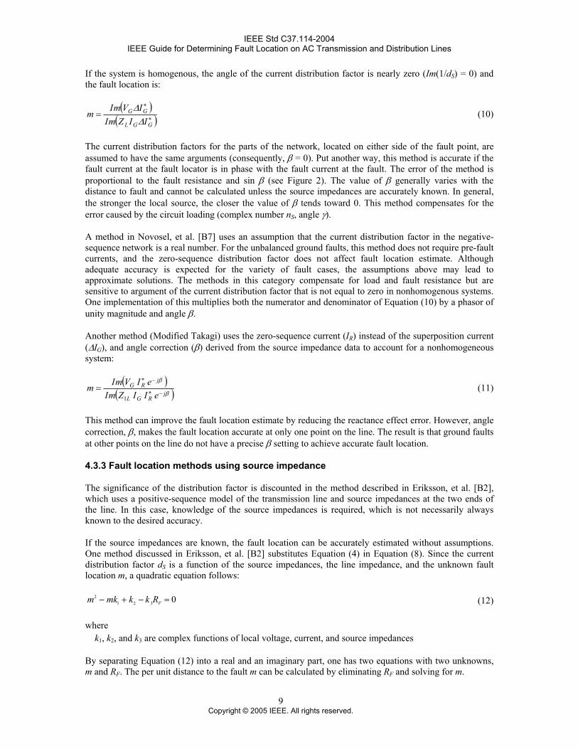
If the system is homogenous, the angle of the current distribution factor is nearly zero (Im(1/dS) = 0) and the fault location is:
( )( )*
*
GGL
GG
IIZmIIVmI
m∆
∆= (10)
The current distribution factors for the parts of the network, located on either side of the fault point, are assumed to have the same arguments (consequently, β = 0). Put another way, this method is accurate if the fault current at the fault locator is in phase with the fault current at the fault. The error of the method is proportional to the fault resistance and sin β (see Figure 2). The value of β generally varies with the distance to fault and cannot be calculated unless the source impedances are accurately known. In general, the stronger the local source, the closer the value of β tends toward 0. This method compensates for the error caused by the circuit loading (complex number nS, angle γ).
A method in Novosel, et al. [B7] uses an assumption that the current distribution factor in the negative-sequence network is a real number. For the unbalanced ground faults, this method does not require pre-fault currents, and the zero-sequence distribution factor does not affect fault location estimate. Although adequate accuracy is expected for the variety of fault cases, the assumptions above may lead to approximate solutions. The methods in this category compensate for load and fault resistance but are sensitive to argument of the current distribution factor that is not equal to zero in nonhomogenous systems. One implementation of this multiplies both the numerator and denominator of Equation (10) by a phasor of unity magnitude and angle β.
Another method (Modified Takagi) uses the zero-sequence current (IR) instead of the superposition current (∆IG), and angle correction (β) derived from the source impedance data to account for a nonhomogeneous system:
( )( )β
β
jRGL
jRG
eIIZmIeIVmIm
−
−=
*1
* (11)
This method can improve the fault location estimate by reducing the reactance effect error. However, angle correction, β, makes the fault location accurate at only one point on the line. The result is that ground faults at other points on the line do not have a precise β setting to achieve accurate fault location.
4.3.3 Fault location methods using source impedance
The significance of the distribution factor is discounted in the method described in Eriksson, et al. [B2], which uses a positive-sequence model of the transmission line and source impedances at the two ends of the line. In this case, knowledge of the source impedances is required, which is not necessarily always known to the desired accuracy.
If the source impedances are known, the fault location can be accurately estimated without assumptions. One method discussed in Eriksson, et al. [B2] substitutes Equation (4) in Equation (8). Since the current distribution factor dS is a function of the source impedances, the line impedance, and the unknown fault location m, a quadratic equation follows:
03212 =−+− FRkkmkm (12)
where k1, k2, and k3 are complex functions of local voltage, current, and source impedances
By separating Equation (12) into a real and an imaginary part, one has two equations with two unknowns, m and RF. The per unit distance to the fault m can be calculated by eliminating RF and solving for m.
9 Copyright © 2005 IEEE. All rights reserved.
IEEE Std C37.114-2004 IEEE Guide for Determining Fault Location on AC Transmission and Distribution Lines
Methods using source impedances are not sensitive to the reactance effect (compensation for load and fault resistance, and argument of current distribution factor) but require the input of the source impedances as the setting parameters. They ensure very accurate results for every network, providing the source impedances are equal to the set value. Errors can occur when the source impedances are not equal to the set values used by the fault locator.
5.
5.1
Two-terminal data methods
Present communications technology allows for use of data from both ends of the transmission line. The calculation of fault location using data from two ends is fundamentally similar to the single-ended methods except now a means exists to determine and minimize or eliminate the effect of fault resistance and other similar factors that tend to throw off the accuracy of the estimate. These factors, such as nontranspositions, strong or weak sources, loading, and others, have been discussed earlier. There have been many articles on variations of the fundamental techniques aimed at improving the accuracy in locating faults. Details of many of these variations can be found in the articles referenced in this guide (i.e., Lawrence, et al. [B10], Aldy, et al. [B11], Hart, et al. [B12], Kezunovic [B13], Novosel, et al. [B14], and Tziouvaras, et al. [B24]).
The two-terminal location methods are more accurate than one-terminal methods and are able to minimize or eliminate the effects of fault resistance, loading, and charging current. Fault type does not need to be calculated. Therefore, positive-sequence components are used rather than zero-sequence, thus eliminating adverse effects of zero-sequence components. The main drawback is the fact that data from both ends must be gathered at one location to be analyzed, whereas the one-terminal location can be done at the line terminal by the relay or other device collecting the data. Effective two-terminal fault location requires an efficient means of collecting oscillographic or phasor data from electronic devices at each end of a line following a fault and processing that data automatically. To simplify the procedure of providing the utility personnel with the proper information at the proper location (such as dispatching center) when needed, the system-wide solution is desirable (see Girgis, et al. [B11]).
This location technique, therefore, takes more time, but speed is not critical for human users. A response in seconds or minutes is adequate. The collected data must also be at least roughly synchronized from each end before analysis is performed. This can be accomplished analytically or through time code stamping. Factors incorporated in the calculations to handle specific error-causing problems may further complicate analysis. Software or other analysis tools are required to properly identify parameters for the fault and implement a two-terminal algorithm. The two-terminal technique has been tested in the field with accurate results (Novosel, et al. [B14]; Peterson, et al. [B29]).
Implementation: data and equipment required
Two-terminal fault location methods require the following equipment for implementation:
⎯ A microprocessor-based relay or other device that measures three-phase voltages and currents at each end with time code.
⎯ Modems and other communications equipment to transfer data to a central site or to the other end of the line.
⎯ Technical personnel or computer equipment at central site for collecting data, performing analysis, and calculating fault location estimate. This may include hardware or software aids.
⎯ Remote communications.
The following data or information is required from the equipment:
⎯ Phase-to-ground voltages and phase currents
⎯ Correlation of time stamps or targeting information within reasonable accuracy to perform phasor calculations on data from both ends
10 Copyright © 2005 IEEE. All rights reserved.
IEEE Std C37.114-2004 IEEE Guide for Determining Fault Location on AC Transmission and Distribution Lines
Software tools enable fault location computation at the level needed by the user (Peterson, et al. [B29]). The tool produces a single value for a location of the fault and a report in a short time after fault occurrence. All fault data are then archived for statistical analysis allowing an improved management of the electrical system. Complexity of the system is hidden to the user considering both generation and analysis of transient data through use of advanced data processing tools. Fault data are processed and analyzed in automated mode and the time required by station engineers for evaluation of each fault is strongly reduced. By using modern data-analysis tools and receiving fault location information when required, the utility personnel can, with much more ease, analyze the status of the electrical power system and reduce duration and number of outages.
Furthermore, Internet and Web-based communication technologies open new possibilities for an enhanced handling of fault data for fault location estimation. Distributed server-client applications may be used to achieve cost-effective and flexible access to fault data. As one of the examples, Web-based computing technology can be applied to access and analyze fault data and calculate fault location simply using the Web browser software on a client PC connected to the Internet. No additional software is needed on this PC.
5.2 System parameters
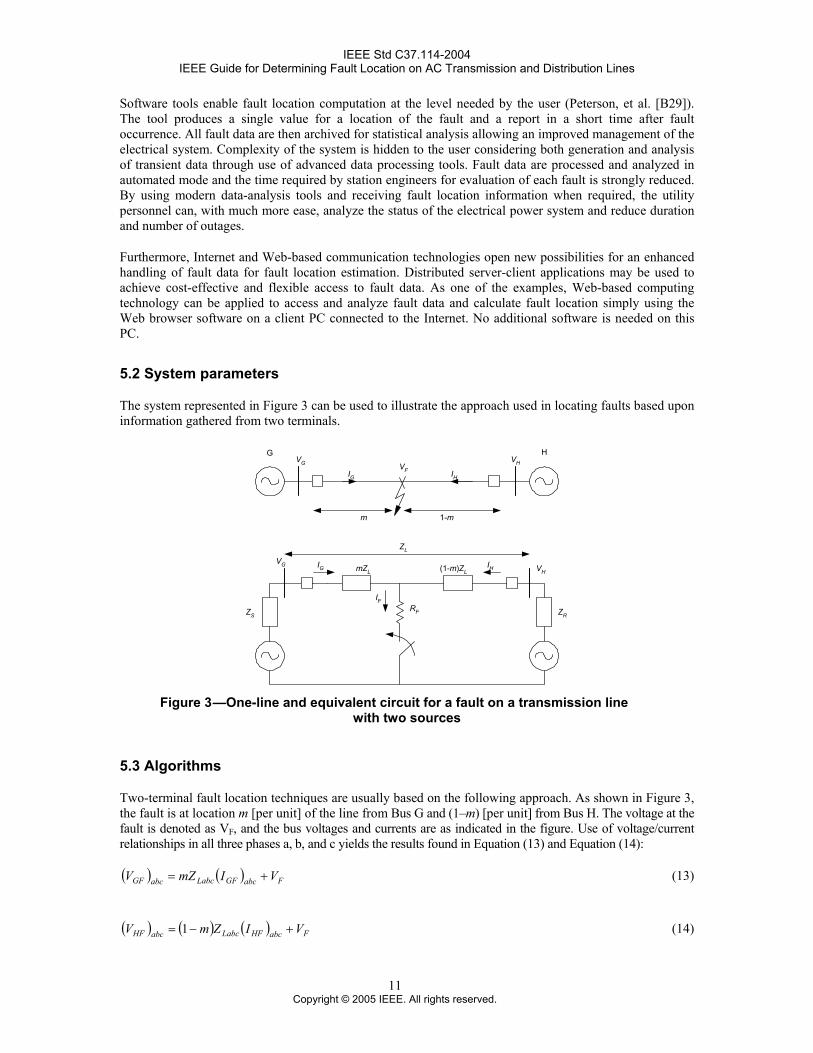
The system represented in Figure 3 can be used to illustrate the approach used in locating faults based upon information gathered from two terminals.
G HVHVF
VG
IG IH
m 1-m
RF
IF
ZL
mZL (1-m)ZLIG IH
ZS ZR
VG VH
Figure 3
5.3
—One-line and equivalent circuit for a fault on a transmission line with two sources
Algorithms
Two-terminal fault location techniques are usually based on the following approach. As shown in Figure 3, the fault is at location m [per unit] of the line from Bus G and (1–m) [per unit] from Bus H. The voltage at the fault is denoted as VF, and the bus voltages and currents are as indicated in the figure. Use of voltage/current relationships in all three phases a, b, and c yields the results found in Equation (13) and Equation (14):
( ) ( ) FabcGFLabcabcGF VImZV += (13)
( ) ( ) ( ) FabcHFLabcabcHF VIZmV +−= 1 (14)
11 Copyright © 2005 IEEE. All rights reserved.
IEEE Std C37.114-2004 IEEE Guide for Determining Fault Location on AC Transmission and Distribution Lines
Subtracting the two equations to eliminate the unknown VF results in Equation (15):
( ) ( ) ( ) ( ) ( )abcHFLabcabcGFLabcabcHFabcGF IZmImZVV 1−+=− (15)
This equation can be solved for the real m, and the phase values can be substituted with the symmetrical components.
6.
6.1
6.2
Other fault location applications
Three-terminal lines
Locating faults on three-terminal lines becomes more complicated but methods have been developed to deal with the problems associated with them (Adly, et al. [B11]), (Tziouvaras, et al. [B24]). One of the first issues to arise when trying to locate faults on three-terminal lines is the setting of the line impedance in the fault locator. The impedance directly from one terminal to either of the other two terminals is chosen. Then, the apparent impedance of the leg to the remaining terminal is determined as a percentage of the original impedance selected. It is important to keep in mind that the apparent impedance will change for different system conditions.
Any faults on the line from the fault locator terminal to the tap point for the three-terminal line should be located correctly. If there is no infeed from the third terminal, the location of faults on the portion of the line beyond the midpoint would also be located correctly. However, any faults from the midpoint to the third terminal or any faults involving infeed would yield results in the fault locator that might be confusing.
A chart or nomograph can be compiled to accommodate the known infeed conditions. If a fault occurs on one of the portions of line beyond the midpoint and the infeed currents are as expected, the fault location can be looked up on the chart or nomograph. There will be two possible locations for the fault. One of the pitfalls for this method is that if the system configuration changes, the infeed currents would be different than anticipated. Thus, the results of the fault locator would no longer correspond to the chart or nomograph and would not be accurate.
If there is a fault locator at each end of a three-terminal line, the fault locator on the section containing the fault is the most accurate of the three.
The method described above requires additional work and analysis to achieve results. Recent techniques (Tziouvaras, et al. [B24]) have been presented that use the negative-sequence network and can convert a three-terminal problem to a more conventional two-terminal one. Fault location can then be solved without any synchronizing requirement.
Series-compensated lines
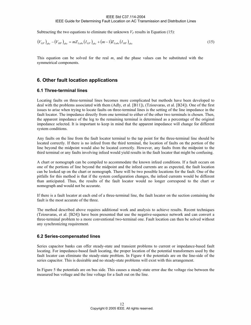
Series capacitor banks can offer steady-state and transient problems to current or impedance-based fault locating. For impedance-based fault locating, the proper location of the potential transformers used by the fault locator can eliminate the steady-state problem. In Figure 4 the potentials are on the line-side of the series capacitor. This is desirable and no steady-state problems will exist with this arrangement. In Figure 5 the potentials are on bus side. This causes a steady-state error due the voltage rise between the measured bus voltage and the line voltage for a fault out on the line.
12 Copyright © 2005 IEEE. All rights reserved.
IEEE Std C37.114-2004 IEEE Guide for Determining Fault Location on AC Transmission and Distribution Lines
FL
Figure 4 —Series-compensated line with line-side voltages
FL
V V'
Zc
Figure 5 —Series-compensated line with
bus side voltages
Consider a fictitious bus on the line side of the capacitor (V'). The voltage at this bus can be calculated using the measured phase currents, voltages, and capacitor impedance as seen in Equation (16):
IZVV C−=' (16)
ZC is a capacitive impedance, at –90 °, which will cause a voltage rise at the fictitious bus compared to the substation bus voltage for current flow out onto the line.
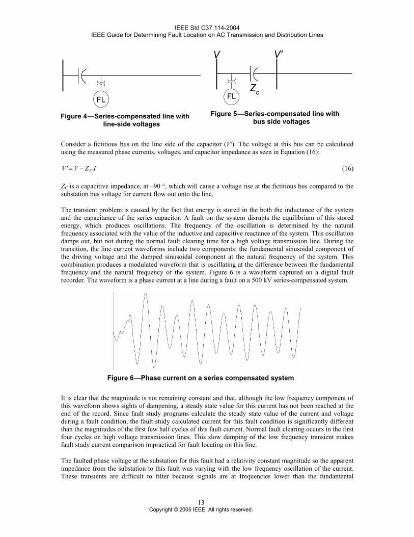
The transient problem is caused by the fact that energy is stored in the both the inductance of the system and the capacitance of the series capacitor. A fault on the system disrupts the equilibrium of this stored energy, which produces oscillations. The frequency of the oscillation is determined by the natural frequency associated with the value of the inductive and capacitive reactance of the system. This oscillation damps out, but not during the normal fault clearing time for a high voltage transmission line. During the transition, the line current waveforms include two components: the fundamental sinusoidal component of the driving voltage and the damped sinusoidal component at the natural frequency of the system. This combination produces a modulated waveform that is oscillating at the difference between the fundamental frequency and the natural frequency of the system. Figure 6 is a waveform captured on a digital fault recorder. The waveform is a phase current at a line during a fault on a 500 kV series-compensated system.
Figure 6 —Phase current on a series compensated system
It is clear that the magnitude is not remaining constant and that, although the low frequency component of this waveform shows sights of dampening, a steady state value for this current has not been reached at the end of the record. Since fault study programs calculate the steady state value of the current and voltage during a fault condition, the fault study calculated current for this fault condition is significantly different than the magnitudes of the first few half cycles of this fault current. Normal fault clearing occurs in the first four cycles on high voltage transmission lines. This slow damping of the low frequency transient makes fault study current comparison impractical for fault locating on this line.
The faulted phase voltage at the substation for this fault had a relativity constant magnitude so the apparent impedance from the substation to this fault was varying with the low frequency oscillation of the current. These transients are difficult to filter because signals are at frequencies lower than the fundamental
13 Copyright © 2005 IEEE. All rights reserved.
IEEE Std C37.114-2004 IEEE Guide for Determining Fault Location on AC Transmission and Distribution Lines
frequency of the system. The oscillation of the apparent impedance makes impedance-based fault locating for this series compensated line impractical.
If the series capacitor’s protection operates (gaps flash) for a fault, the oscillations are damped quickly and impedance or current-based fault locating will provide fault locating as accurate as for other uncompensated lines. The system from which the waveform in Figure 6 was recorded has two 67 Ω series capacitors in the line and there are large sections of the line for which faults will not cause [one or neither] of the capacitor banks’ gaps to flash.
The low frequency oscillations of the current produces peak values that are higher than the predicted steady state fault current. The higher currents cause the protection on the series capacitor bank to operate for faults in locations the steady state studies would not have predicted. If the series capacitor bank is protected with gaps, the capacitor bank would be completely shunted when the protection operates, but if it is protected with metal oxide varistors (MOVs) the capacitor bank is only shunted during the current peak values. The operation of the MOVs creates impedance for the capacitor bank that looks like a variable resistor in parallel with a capacitor. The value of the variable resistor is changing during the waveform of the current through the series capacitor bank. If the location of the fault is trying to be determined by monitoring the current that is passing through the capacitor bank, the results are disappointing.
Fault locating using current or impedance measuring methods has proven to give some degree of accuracy if the impedance of the bank is relatively small and the protection limit of the capacitor is low compared to the available fault current. The following is an example of such a case.
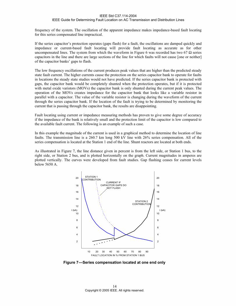
In this example the magnitude of the current is used in a graphical method to determine the location of line faults. The transmission line is a 260.7 km long 500 kV line with 26% series compensation. All of the series compensation is located at the Station 1 end of the line. Shunt reactors are located at both ends.
As illustrated in Figure 7, the line distance given in percent is from the left side, or Station 1 bus, to the right side, or Station 2 bus, and is plotted horizontally on the graph. Current magnitudes in amperes are plotted vertically. The curves were developed from fault studies. Gap flashing ceases for current levels below 5650 A.
I (kA)
2
4
6
8
10
12
14
16
18
20
2
4
6
8
10
12
14
16
18
20
40 9010 5020 30 60 70 80
STATION 1CONTRIBUTION
STATION 2CONTRIBUTION
CURRENT IFCAPACITOR GAPS DO
NOT FLASH
I (kA)
FAULT LOCATION IN % FROM STATION 1 BUS Figure 7 —Series compensation located at one end only
14 Copyright © 2005 IEEE. All rights reserved.
IEEE Std C37.114-2004 IEEE Guide for Determining Fault Location on AC Transmission and Distribution Lines
Using only a single end current contribution curve may not provide sufficient information to locate a particular fault. For example, using only fault recorder information from Station 1, it can be seen that for a 5000 A fault, two possible fault locations exist. One location could be at 32% of the line if the gaps flash and another at 53% if the gaps do not flash.
Since the location of the fault may plot at different distances, depending on which current contribution curve is used, a midpoint between the two values is chosen as the probable location. For example, using Figure 7, if the location plots at 40% of the Station 2 current contribution curve (2800 A) and the location plots at 30% on the Station 1 current contribution curve (5200 A), then the fault location is selected as at 35% of the transmission line. Ideally, the Station 2 current contribution should be 2400 A. However, error due to differences in calculated impedance from actual line impedance affects the true value.
Annex B provides additional theoretical information on series-compensated lines.
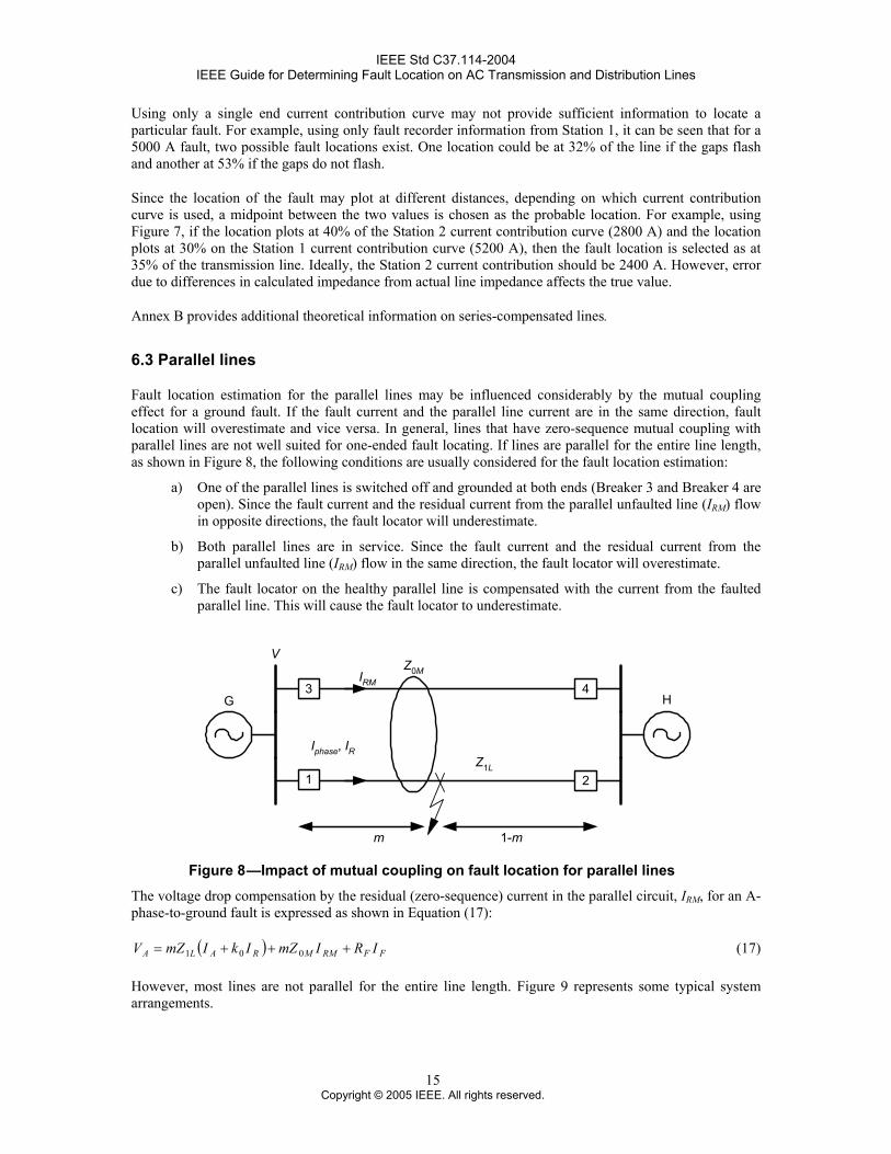
6.3 Parallel lines
Fault location estimation for the parallel lines may be influenced considerably by the mutual coupling effect for a ground fault. If the fault current and the parallel line current are in the same direction, fault location will overestimate and vice versa. In general, lines that have zero-sequence mutual coupling with parallel lines are not well suited for one-ended fault locating. If lines are parallel for the entire line length, as shown in Figure 8, the following conditions are usually considered for the fault location estimation:
a) One of the parallel lines is switched off and grounded at both ends (Breaker 3 and Breaker 4 are open). Since the fault current and the residual current from the parallel unfaulted line (IRM) flow in opposite directions, the fault locator will underestimate.
b) Both parallel lines are in service. Since the fault current and the residual current from the parallel unfaulted line (IRM) flow in the same direction, the fault locator will overestimate.
c) The fault locator on the healthy parallel line is compensated with the current from the faulted parallel line. This will cause the fault locator to underestimate.
G H
V
Iphase, IR
m 1-m
IRM
Z0M
3
Z1L1
4
2
Figure 8 —Impact of mutual coupling on fault location for parallel lines
The voltage drop compensation by the residual (zero-sequence) current in the parallel circuit, IRM, for an A-phase-to-ground fault is expressed as shown in Equation (17):
( ) FFRMMRALA IRImZIkImZV +++= 001 (17)
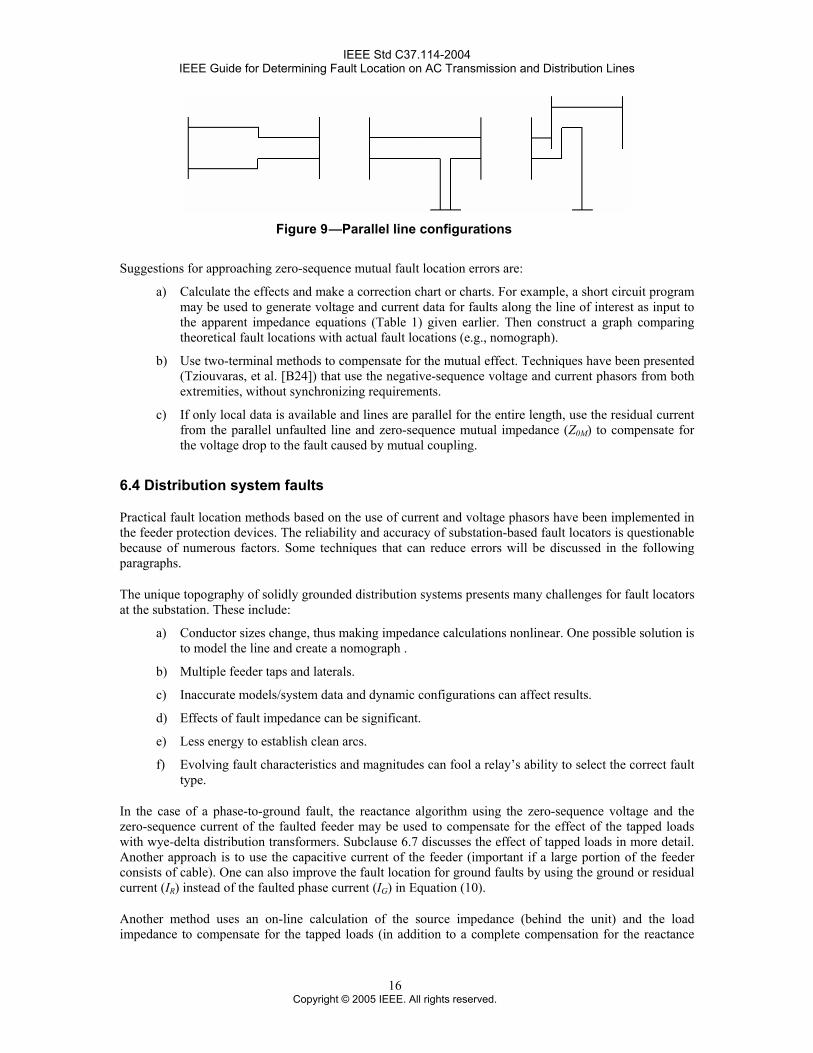
However, most lines are not parallel for the entire line length. Figure 9 represents some typical system arrangements.
15 Copyright © 2005 IEEE. All rights reserved.
IEEE Std C37.114-2004 IEEE Guide for Determining Fault Location on AC Transmission and Distribution Lines
Figure 9
6.4
—Parallel line configurations
Suggestions for approaching zero-sequence mutual fault location errors are:
a) Calculate the effects and make a correction chart or charts. For example, a short circuit program may be used to generate voltage and current data for faults along the line of interest as input to the apparent impedance equations (Table 1) given earlier. Then construct a graph comparing theoretical fault locations with actual fault locations (e.g., nomograph).
b) Use two-terminal methods to compensate for the mutual effect. Techniques have been presented (Tziouvaras, et al. [B24]) that use the negative-sequence voltage and current phasors from both extremities, without synchronizing requirements.
c) If only local data is available and lines are parallel for the entire length, use the residual current from the parallel unfaulted line and zero-sequence mutual impedance (Z0M) to compensate for the voltage drop to the fault caused by mutual coupling.
Distribution system faults
Practical fault location methods based on the use of current and voltage phasors have been implemented in the feeder protection devices. The reliability and accuracy of substation-based fault locators is questionable because of numerous factors. Some techniques that can reduce errors will be discussed in the following paragraphs.
The unique topography of solidly grounded distribution systems presents many challenges for fault locators at the substation. These include:
a) Conductor sizes change, thus making impedance calculations nonlinear. One possible solution is to model the line and create a nomograph .
b) Multiple feeder taps and laterals.
c) Inaccurate models/system data and dynamic configurations can affect results.
d) Effects of fault impedance can be significant.
e) Less energy to establish clean arcs.
f) Evolving fault characteristics and magnitudes can fool a relay’s ability to select the correct fault type.
In the case of a phase-to-ground fault, the reactance algorithm using the zero-sequence voltage and the zero-sequence current of the faulted feeder may be used to compensate for the effect of the tapped loads with wye-delta distribution transformers. Subclause 6.7 discusses the effect of tapped loads in more detail. Another approach is to use the capacitive current of the feeder (important if a large portion of the feeder consists of cable). One can also improve the fault location for ground faults by using the ground or residual current (IR) instead of the faulted phase current (IG) in Equation (10).
Another method uses an on-line calculation of the source impedance (behind the unit) and the load impedance to compensate for the tapped loads (in addition to a complete compensation for the reactance
16 Copyright © 2005 IEEE. All rights reserved.
IEEE Std C37.114-2004 IEEE Guide for Determining Fault Location on AC Transmission and Distribution Lines
effect) in a radial distribution network. The load impedance is calculated using the pre-fault data shown in Equation (18):
ll
l ZIV
Z load −= (18)
where lV and are pre-fault load voltage and current lI
Source impedance behind the fault locator is calculated from the fault and pre-fault voltages and currents at the terminal as shown in Equation (19):
G
GS I
VZ
∆∆
−= (19)
Since the system is radial, by calculating and ZS, the value of β is accurately calculated as shown in Equation (3). Once the value of β is accurately known, this method (using only local measurements) can compensate completely for the errors caused by the reactance effect without requiring input of a source impedance as a setting parameter. Compensation for tapped loads allows this method to provide accurate results for a variety of fault cases on distribution feeders, although the accuracy may degrade for faults occurring toward the end of the feeder.
lZ
Distribution networks can have different grounding principles, which affect the means to determine fault location. Grounding principles can be as follows:
a) Solidly grounded
b) Ungrounded networks
c) Peterson’s coil
d) Resistance grounded
6.4.1
6.4.1.1
Solidly grounded networks
Of the four types of grounding listed above, the solidly grounded network is the most common in North America. The ungrounded network will require grounding transformers, which are distributed around the network resulting in fewer sources of ground current. The net effect of this and of the latter two types of grounding is to reduce the magnitude of the ground current. This can be seen as an increase in zero-sequence source impedance. Techniques to locate faults on these networks will not differ from those shown for solidly grounded networks except for the reduced accuracy of the computational techniques.
Traditional methodologies
Often faults are located without the use of any measurements. Location is simply made through physical indications, field methods, and brute force methods such as:
a) Restoration through switching
b) Restoration through recloser operation
c) Indication through fuse and fault locator operation
d) Downed wires, customer calls, maps
e) Relay targets
f) DC thumping of underground circuits
g) Smelling burnt cables
17 Copyright © 2005 IEEE. All rights reserved.
IEEE Std C37.114-2004 IEEE Guide for Determining Fault Location on AC Transmission and Distribution Lines
6.4.1.2
6.4.1.3
6.5
6.5.1
Observant technologies
The ability to collect data further improves upon the success of locating faults through such techniques as:
a) Local detection with communications feedback
b) “Fault was upstream or downstream”
c) Intelligent metering with modem, cellular-based devices, LOCATE-type devices
d) Detectors sending feedback through SCADA
e) Satellite-based location or carrier packages
f) Choice of passing on information to an “interpreter” (i.e., a person) or to an “interpretive device” (i.e., a substation HMI or DMS)
g) Fault recorders
Intelligent technologies
Due to complexity, intelligent technologies are being applied for distribution fault location. These include:
a) Artificial intelligence, neural networks to “learn” system characteristics
b) Distributed intelligence in substations to pull together information for best guess, confidence factors
Although evolving, competition may arise among observant technologies dispersed throughout the system, but integrated together, and advanced intelligent technologies.
Locating faults on underground cables, paralleled cable circuits
Underground cables
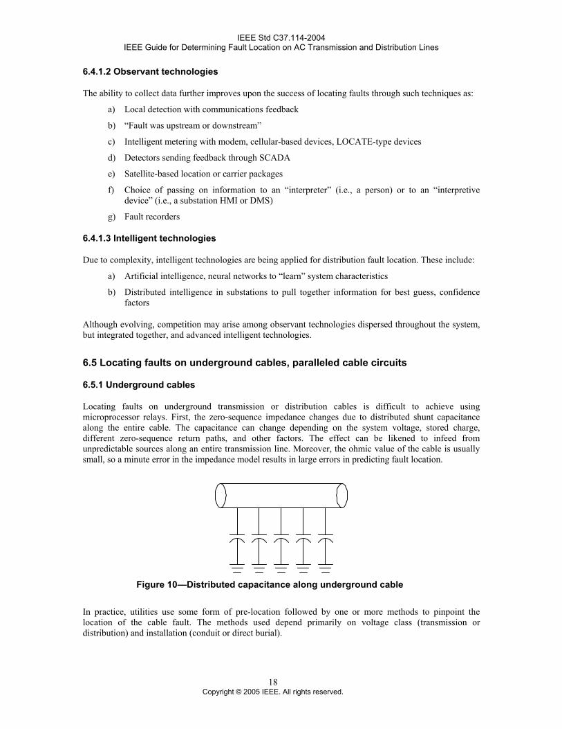
Locating faults on underground transmission or distribution cables is difficult to achieve using microprocessor relays. First, the zero-sequence impedance changes due to distributed shunt capacitance along the entire cable. The capacitance can change depending on the system voltage, stored charge, different zero-sequence return paths, and other factors. The effect can be likened to infeed from unpredictable sources along an entire transmission line. Moreover, the ohmic value of the cable is usually small, so a minute error in the impedance model results in large errors in predicting fault location.
Figure 10—Distributed capacitance along underground cable
In practice, utilities use some form of pre-location followed by one or more methods to pinpoint the location of the cable fault. The methods used depend primarily on voltage class (transmission or distribution) and installation (conduit or direct burial).
18 Copyright © 2005 IEEE. All rights reserved.
IEEE Std C37.114-2004 IEEE Guide for Determining Fault Location on AC Transmission and Distribution Lines
There are generally two categories of fault locating: terminal methods and tracer methods. These methods of fault locating usually take place after a fault has occurred and has been cleared by protective relaying.
Terminal methods measure electrical quantities at one or both ends of the cable circuit. Terminal methods are usually used to “pre-locate” the fault. The most popular terminal methods include “bridge” techniques, like the Murray Loop, and Radar/Low or High Voltage pulse methods (Bascom, et al. [B16]).
Tracer methods are most useful for “pinpointing” the location of the fault, and usually require walking the cable route in the field. The most popular tracer methods are acoustic (“thumper”) techniques and earth gradient (applying a source and measuring return current) methods, although many other methods are used (Bascom, et al. [B16]).
Recent developments in using the transient voltage and current waves during a fault have improved pinpointing cable fault location on distribution circuits. The method measures the time between transient peaks to compute a distance to fault (Wiggins [B17]).
6.5.2 Paralleled cable circuits
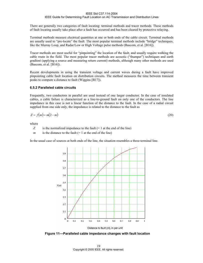
Frequently, two conductors in parallel are used instead of one larger conductor. In the case of insulated cables, a cable failure is characterized as a line-to-ground fault on only one of the conductors. The line impedance in this case is not a linear function of the distance to the fault. In the case of a radial circuit supplied from one side only, the impedance is related to the distance to the fault as
( ) ( )mmmfZ −== 2 (20)
where Z is the normalized impedance to the fault (= 1 at the end of the line) m is the distance to the fault (= 1 at the end of the line)
In the usual case of sources at both ends of the line, the situation resembles a three-terminal line.
Figure 11—Paralleled cable impedance changes with fault location
19 Copyright © 2005 IEEE. All rights reserved.
IEEE Std C37.114-2004 IEEE Guide for Determining Fault Location on AC Transmission and Distribution Lines
6.6
6.7
Automatic reclosing effects on fault locating
Automatic reclosing can affect the accuracy of fault locating, depending on the line configuration. The first fault usually provides accurate data because it usually has valid pre-fault and fault data. If reclosing into a de-energized line, the absence of load can actually help produce a more accurate fault location estimate, as long as the fault locator selects the correct data. Both two-terminal and one-terminal algorithms can be applied to locate faults. Automatic or supervisory reclose attempts into a permanent fault can (and most often do) have increased dc offset that can take several cycles to decay. This dc offset must be accounted for (e.g., filtering relay inputs) in order to accurately locate the fault.
Effect of tapped load
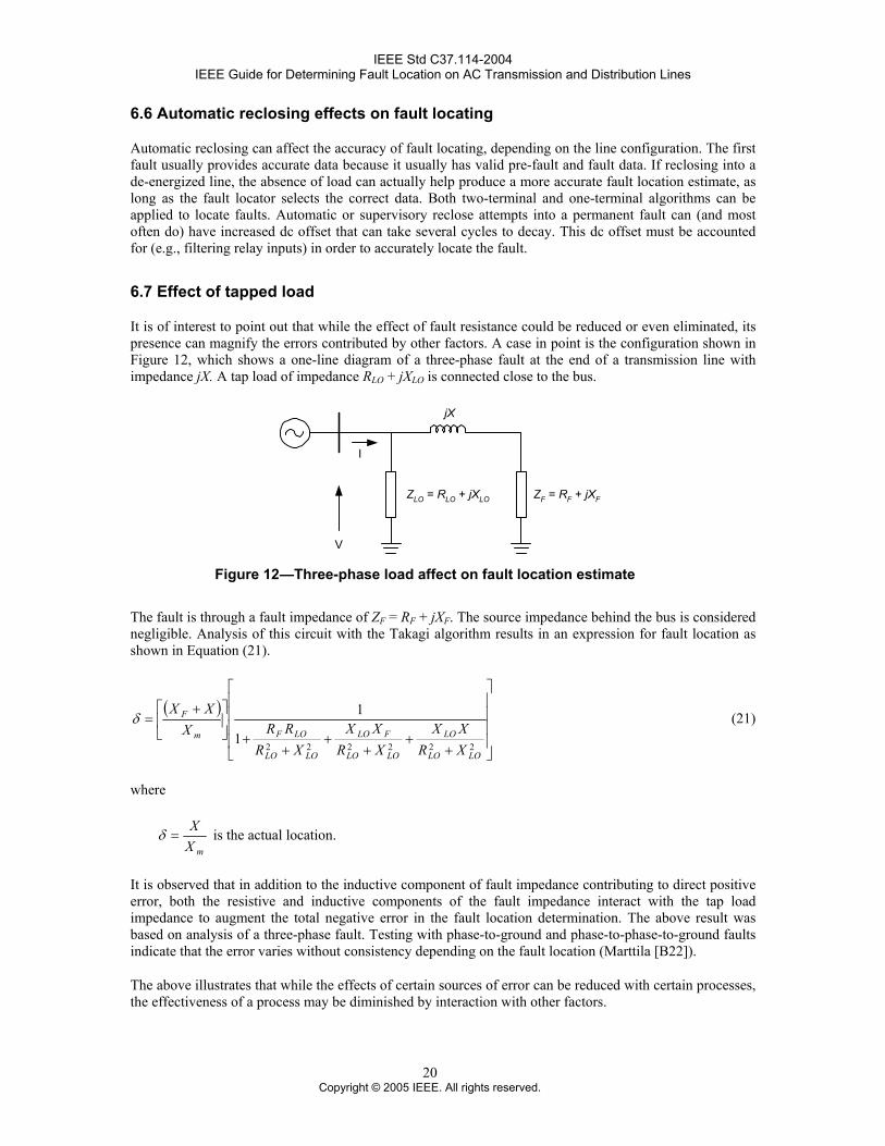
It is of interest to point out that while the effect of fault resistance could be reduced or even eliminated, its presence can magnify the errors contributed by other factors. A case in point is the configuration shown in Figure 12, which shows a one-line diagram of a three-phase fault at the end of a transmission line with impedance jX. A tap load of impedance RLO + jXLO is connected close to the bus.
jX
ZF = RF + jXFZLO = RLO + jXLO
I
V Figure 12—Three-phase load affect on fault location estimate
The fault is through a fault impedance of ZF = RF + jXF. The source impedance behind the bus is considered negligible. Analysis of this circuit with the Takagi algorithm results in an expression for fault location as shown in Equation (21).
( )
⎥⎥⎥⎥
⎦
⎤
⎢⎢⎢⎢
⎣
⎡
++
++
++
⎥⎦
⎤⎢⎣
⎡ +=
2222221
1
LOLO
LO
LOLO
FLO
LOLO
LOFm
F
XRXX
XRXX
XRRRX
XXδ (21)
where
mXX
=δ is the actual location.
It is observed that in addition to the inductive component of fault impedance contributing to direct positive error, both the resistive and inductive components of the fault impedance interact with the tap load impedance to augment the total negative error in the fault location determination. The above result was based on analysis of a three-phase fault. Testing with phase-to-ground and phase-to-phase-to-ground faults indicate that the error varies without consistency depending on the fault location (Marttila [B22]).
The above illustrates that while the effects of certain sources of error can be reduced with certain processes, the effectiveness of a process may be diminished by interaction with other factors.
20 Copyright © 2005 IEEE. All rights reserved.
IEEE Std C37.114-2004 IEEE Guide for Determining Fault Location on AC Transmission and Distribution Lines
6.8
6.9
6.10
Phase selection, fault identification, sequential faults
Fault location algorithms in protective relays typically use pre-fault and fault currents measured locally and stored in the memory of the relay. Under normal system conditions, the relay is measuring the currents and voltages for all phases and storing them in a buffer. Once the relay detects a fault condition in the zone of protection or initiates a trip of the line breaker(s), the data in the buffer are not updated any more and are used to perform the fault location calculations.
The next step in a typical algorithm is the selection of current and voltage data to be used for the fault location calculation. A different loop is selected as a function of a faulted phase selection procedure. Many algorithms make the faulted phase selection based on superimposed components, this way eliminating the effect of the load on the phase selection.
The faulted phase selection decision is very important because if the wrong loop is selected, the results from the fault location algorithm will not be accurate. It will affect the calculation also because it is used in the determination of the fault inception point. A certain number of samples before and after the fault inception will be used to calculate the voltage and current phasors. If the faulted phase and fault inception point are not correctly selected, the calculated phasors will also introduce error in the estimation of the fault location.
Evolving faults introduce an additional problem, since they will usually require a switch from a single-phase-to-ground loop to a phase-to-phase loop. Two-phase-to-ground faults are typically evaluated as phase-to-phase faults in a fault location algorithm.
A three-phase or three-phase-to-ground fault can be considered as a combination of three phase-to-phase faults. The fault location is then determined for each phase-to-phase fault, and the closest to the relay location or the average of the three can be used as the output from the fault location algorithm. Some fault location algorithms may instead use a pre-selected phase-to-phase loop (for example a-b) in case of a three-phase fault.
Some relays use the same algorithm for fault location that is used by the distance protection function, but with a higher number of samples, which results in a better accuracy. Appropriate faulted phase selection is important in this case as well, because the resistance and reactance calculation is based on a single-phase or two-phase loop.
Long lines and reactor and capacitor installations
Long transmission lines on higher voltage levels may exhibit considerable capacitance resulting in a significant charging current. Shunt reactors or capacitors may be installed in the substations. If the fault location algorithms (one-terminal and two-terminal) do not compensate for the shunt elements and the charging currents, an error may be introduced. Improvements in estimation can be accomplished by:
a) Compensation for charging currents and shunt reactors or capacitors by using a Π, Γ, or T line model
b) Compensation for long lines using a distributed line model
Short duration faults
Impedance-based fault locating methods require that the fundamental voltage and current quantities be accurately measured. This requires signal filtering and signals of long enough duration to measure. If faults clear faster than two cycles, the current may never reach its faulted steady state, and the voltage may never drop to its faulted steady-state, so the fault locator tends to estimate long. Traveling-wave approaches may provide the only solutions.
21 Copyright © 2005 IEEE. All rights reserved.
IEEE Std C37.114-2004 IEEE Guide for Determining Fault Location on AC Transmission and Distribution Lines
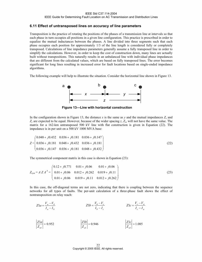
6.11 Effect of untransposed lines on accuracy of line parameters
Transposition is the practice of rotating the positions of the phases of a transmission line at intervals so that each phase in turn occupies all positions in a given line configuration. This practice is prescribed in order to equalize the mutual inductances between the phases. A line divided into three segments such that each phase occupies each position for approximately 1/3 of the line length is considered fully or completely transposed. Calculations of line impedance parameters generally assume a fully transposed line in order to simplify the calculations. However, in order to keep the cost of construction down, many lines are actually built without transpositions. This naturally results in an unbalanced line with individual phase impedances that are different from the calculated values, which are based on fully transposed lines. The error becomes significant for long lines resulting in increased error for fault locations based on single-ended impedance algorithms.
The following example will help to illustrate the situation. Consider the horizontal line shown in Figure 13.
a b c
zx y
Figure 13—Line with horizontal construction
In the configuration shown in Figure 13, the distance x is the same as y and the mutual impedances Zx and Zy are expected to be equal. However, because of the wider spacing z, Zzc will not have the same value. The matrix for a 162-km untransposed 500 kV line with flat construction is given in Equation (22). The impedance is in per unit on a 500 kV 1000 MVA base:
Z = (22) ⎟⎟⎟⎟
⎠
⎞
⎜⎜⎜⎜
⎝
⎛
+++
+++
+++
432.0048.0181.0036.0147.0036.0
181.0036.0432.0048.0181.0036.0
147.0036.0181.0036.0432.0048.0
jjj
jjj
jjj
The symmetrical component matrix in this case is shown in Equation (23):
Zsym = A Z A-1 = (23) ⎟⎟⎟⎟
⎠
⎞
⎜⎜⎜⎜
⎝
⎛
+++
+++
+++
262.0012.011.0019.006.001.0
11.0019.0262.0012.006.001.0
06.001.006.001.0771.012.0
jjj
jjj
jjj
In this case, the off-diagonal terms are not zero, indicating that there is coupling between the sequence networks for all types of faults. The per-unit calculation of a three-phase fault shows the effect of nontransposition on relay reach:
ba
ba
IIVV
aZ−−
=1 cb
cb
IIVV
bZ−−
=1 ac
ac
IIVV
cZ−−
=1
952.01
1=
aZaZ 946.01
1=
aZbZ 085.11
1=
aZcZ
22 Copyright © 2005 IEEE. All rights reserved.
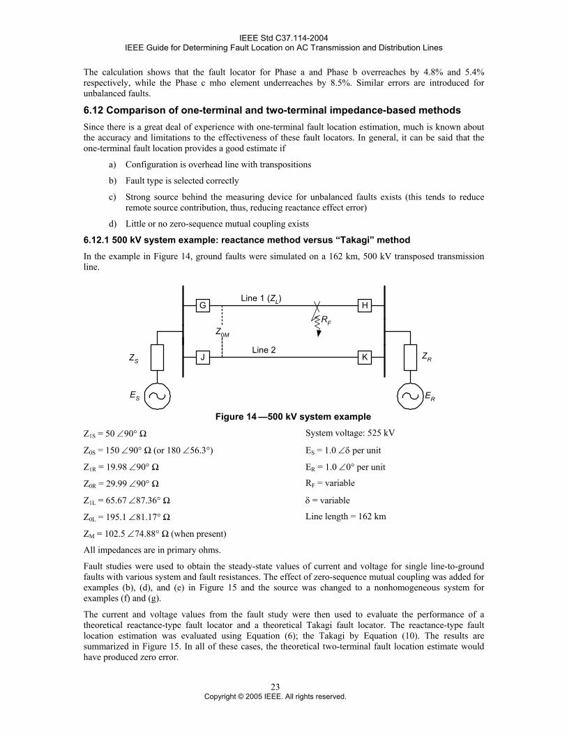
IEEE Std C37.114-2004 IEEE Guide for Determining Fault Location on AC Transmission and Distribution Lines
The calculation shows that the fault locator for Phase a and Phase b overreaches by 4.8% and 5.4% respectively, while the Phase c mho element underreaches by 8.5%. Similar errors are introduced for unbalanced faults.
6.12
6.12.1
Comparison of one-terminal and two-terminal impedance-based methods Since there is a great deal of experience with one-terminal fault location estimation, much is known about the accuracy and limitations to the effectiveness of these fault locators. In general, it can be said that the one-terminal fault location provides a good estimate if
a) Configuration is overhead line with transpositions
b) Fault type is selected correctly
c) Strong source behind the measuring device for unbalanced faults exists (this tends to reduce remote source contribution, thus, reducing reactance effect error)
d) Little or no zero-sequence mutual coupling exists
500 kV system example: reactance method versus “Takagi” method
In the example in Figure 14, ground faults were simulated on a 162 km, 500 kV transposed transmission line.
H
K
G
J
Line 1 (ZL)
Line 2
ES
ZR
ER
Z0M
RF
ZS
Figure 14 —500 kV system example
Z1S = 50 ∠90° Ω System voltage: 525 kV
Z0S = 150 ∠90° Ω (or 180 ∠56.3°) ES = 1.0 ∠δ per unit
Z1R = 19.98 ∠90° Ω ER = 1.0 ∠0° per unit
Z0R = 29.99 ∠90° Ω RF = variable
Z1L = 65.67 ∠87.36° Ω δ = variable
Z0L = 195.1 ∠81.17° Ω Line length = 162 km
ZM = 102.5 ∠74.88° Ω (when present)
All impedances are in primary ohms.
Fault studies were used to obtain the steady-state values of current and voltage for single line-to-ground faults with various system and fault resistances. The effect of zero-sequence mutual coupling was added for examples (b), (d), and (e) in Figure 15 and the source was changed to a nonhomogeneous system for examples (f) and (g).
The current and voltage values from the fault study were then used to evaluate the performance of a theoretical reactance-type fault locator and a theoretical Takagi fault locator. The reactance-type fault location estimation was evaluated using Equation (6); the Takagi by Equation (10). The results are summarized in Figure 15. In all of these cases, the theoretical two-terminal fault location estimate would have produced zero error.
23 Copyright © 2005 IEEE. All rights reserved.
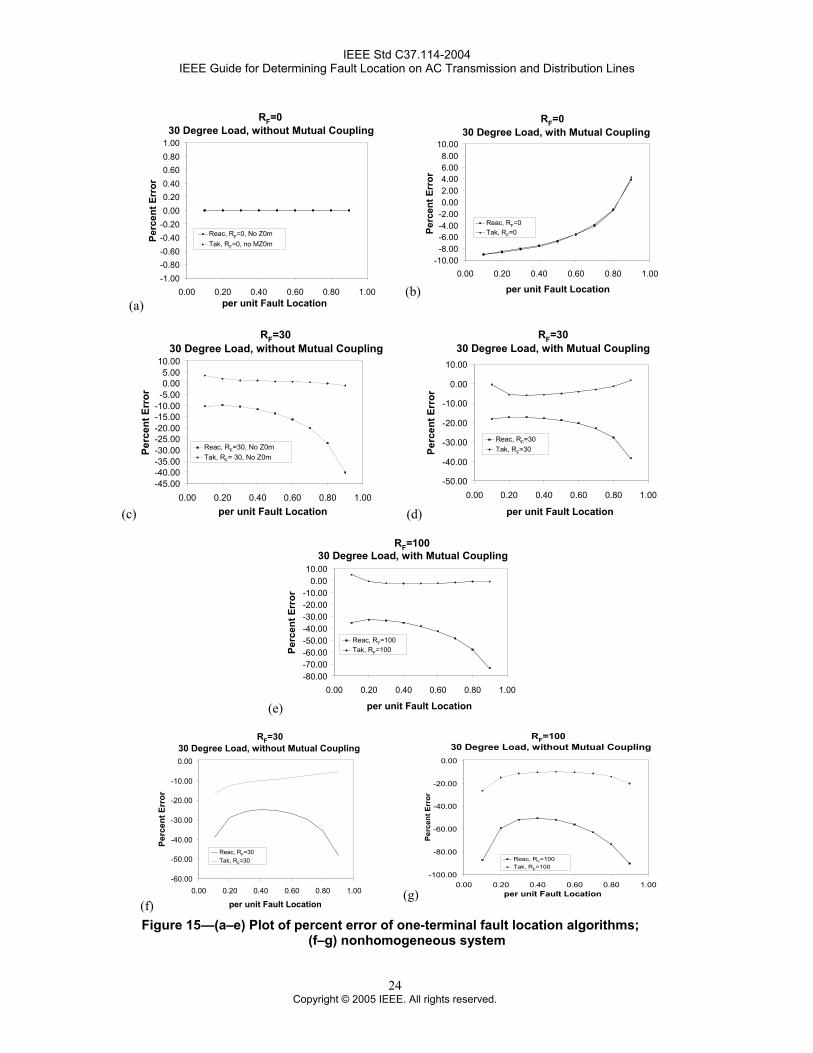
IEEE Std C37.114-2004 IEEE Guide for Determining Fault Location on AC Transmission and Distribution Lines
(a)
RF=030 Degree Load, without Mutual Coupling
-1.00-0.80-0.60-0.40-0.200.000.200.400.600.801.00
0.00 0.20 0.40 0.60 0.80 1.00per unit Fault Location
Perc
ent E
rror
Reac, RF=0, No Z0mTak, RF=0, no MZ0m
(b)
30 Degree Load, with Mutual Coupling
-10.00-8.00-6.00-4.00-2.000.002.004.006.008.00
10.00
0.00 0.20 0.40 0.60 0.80 1.00
per unit Fault Location
Perc
ent E
rror
Reac, RF=0Tak, RF=0
RF=0
(c)
RF=3030 Degree Load, without Mutual Coupling
-45.00-40.00-35.00-30.00-25.00-20.00-15.00-10.00-5.000.005.00
10.00
0.00 0.20 0.40 0.60 0.80 1.00per unit Fault Location
Perc
ent E
rror
Reac, RF=30, No Z0mTak, RF= 30, No Z0m
(d)
RF=3030 Degree Load, with Mutual Coupling
-50.00
-40.00
-30.00
-20.00
-10.00
0.00
10.00
0.00 0.20 0.40 0.60 0.80 1.00
per unit Fault Location
Perc
ent E
rror
Reac, RF=30Tak, RF=30
(e)
RF=10030 Degree Load, with Mutual Coupling
-80.00-70.00-60.00-50.00-40.00-30.00-20.00-10.00
0.0010.00
0.00 0.20 0.40 0.60 0.80 1.00
per unit Fault Location
Perc
ent E
rror
Reac, RF=100Tak, RF=100
(f)
RF=3030 Degree Load, without Mutual Coupling
-60.00
-50.00
-40.00
-30.00
-20.00
-10.00
0.00
0.00 0.20 0.40 0.60 0.80 1.00
per unit Fault Location
Perc
ent E
rror
Reac, RF=30Tak, RF=30
(g)
RF=10030 Degree Load, without Mutual Coupling
-100.00
-80.00
-60.00
-40.00
-20.00
0.00
0.00 0.20 0.40 0.60 0.80 1.00per unit Fault Location
Perc
ent E
rror
Reac, RF=100Tak, RF=100
Figure 15—(a–e) Plot of percent error of one-terminal fault location algorithms; (f–g) nonhomogeneous system
24 Copyright © 2005 IEEE. All rights reserved.
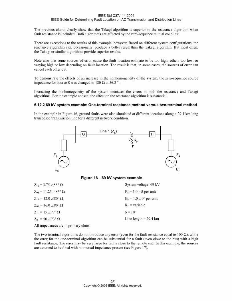
IEEE Std C37.114-2004 IEEE Guide for Determining Fault Location on AC Transmission and Distribution Lines
The previous charts clearly show that the Takagi algorithm is superior to the reactance algorithm when fault resistance is included. Both algorithms are affected by the zero-sequence mutual coupling.
There are exceptions to the results of this example, however. Based on different system configurations, the reactance algorithm can, occasionally, produce a better result than the Takagi algorithm. But most often, the Takagi or similar algorithms provide superior results.
Note also that some sources of error cause the fault location estimate to be too high, others too low, or varying high or low depending on fault location. The result is that, in some cases, the sources of error can cancel each other out.
To demonstrate the effects of an increase in the nonhomogeneity of the system, the zero-sequence source impedance for source S was changed to 180 Ω at 56.3 °.
Increasing the nonhomogeneity of the system increases the errors in both the reactance and Takagi algorithms. For the example chosen, the effect on the reactance algorithm is substantial.
6.12.2 69 kV system example: One-terminal reactance method versus two-terminal method
In the example in Figure 16, ground faults were also simulated at different locations along a 29.4 km long transposed transmission line for a different network condition.
HGLine 1 (ZL)
ES
ZR
ER
RF
ZS
Figure 16—69 kV system example
Z1S = 3.75 ∠86° Ω System voltage: 69 kV
Z0S = 11.25 ∠86° Ω ES = 1.0 ∠δ per unit
Z1R = 12.0 ∠80° Ω ER = 1.0 ∠0° per unit
Z0R = 36.0 ∠80° Ω RF = variable
Z1L = 15 ∠77° Ω δ = 10°
Z0L = 50 ∠73° Ω Line length = 29.4 km
All impedances are in primary ohms.
The two-terminal algorithms do not introduce any error (even for the fault resistance equal to 100 Ω), while the error for the one-terminal algorithm can be substantial for a fault (even close to the bus) with a high fault resistance. The error may be very large for faults close to the remote end. In this example, the sources are assumed to be fixed with no mutual impedance present (see Figure 17).
25 Copyright © 2005 IEEE. All rights reserved.
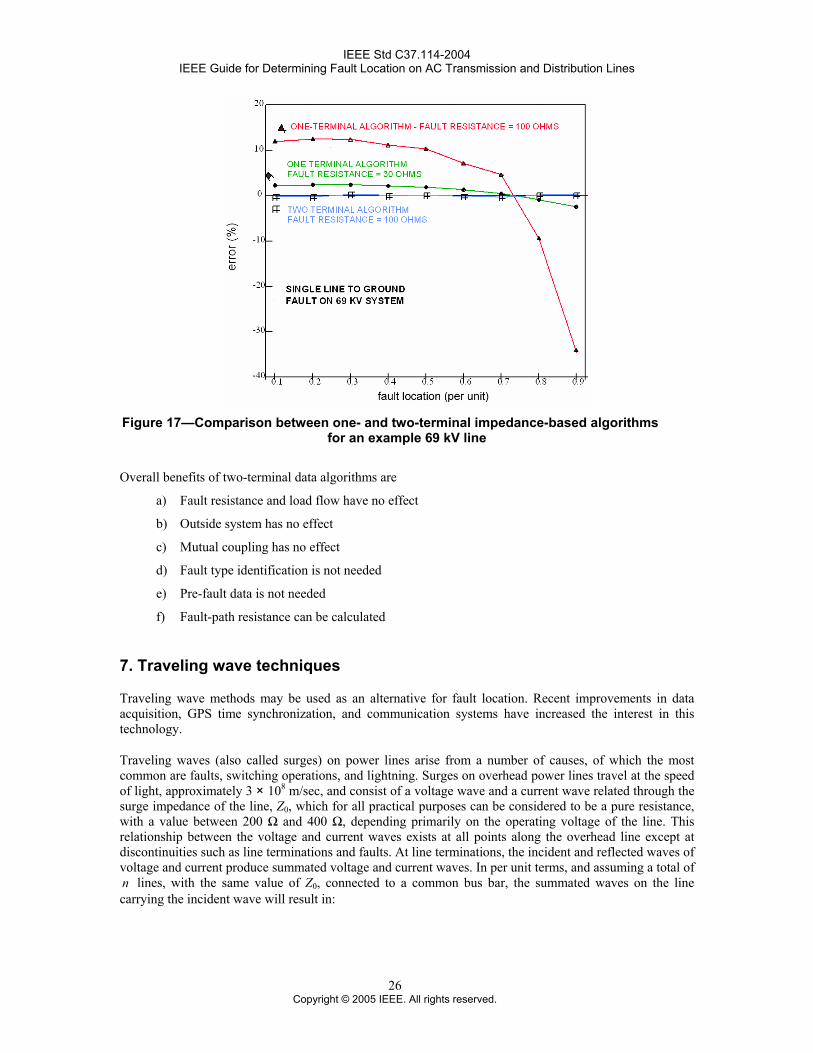
IEEE Std C37.114-2004 IEEE Guide for Determining Fault Location on AC Transmission and Distribution Lines
Figure 17
7.
n
—Comparison between one- and two-terminal impedance-based algorithms for an example 69 kV line
Overall benefits of two-terminal data algorithms are
a) Fault resistance and load flow have no effect
b) Outside system has no effect
c) Mutual coupling has no effect
d) Fault type identification is not needed
e) Pre-fault data is not needed
f) Fault-path resistance can be calculated
Traveling wave techniques
Traveling wave methods may be used as an alternative for fault location. Recent improvements in data acquisition, GPS time synchronization, and communication systems have increased the interest in this technology.
Traveling waves (also called surges) on power lines arise from a number of causes, of which the most common are faults, switching operations, and lightning. Surges on overhead power lines travel at the speed of light, approximately 3 × 10⁸ m/sec, and consist of a voltage wave and a current wave related through the surge impedance of the line, Z0, which for all practical purposes can be considered to be a pure resistance, with a value between 200 Ω and 400 Ω, depending primarily on the operating voltage of the line. This relationship between the voltage and current waves exists at all points along the overhead line except at discontinuities such as line terminations and faults. At line terminations, the incident and reflected waves of voltage and current produce summated voltage and current waves. In per unit terms, and assuming a total of
lines, with the same value of Z0, connected to a common bus bar, the summated waves on the line carrying the incident wave will result in:
26 Copyright © 2005 IEEE. All rights reserved.
IEEE Std C37.114-2004 IEEE Guide for Determining Fault Location on AC Transmission and Distribution Lines
n2 WaveVoltage Summated =
nn )22(
veCurrent Wa Summated−
= (24)
From the above, Equation (24) we can see that as the number of lines connected to a bus bar increases, the summated voltage wave will tend to zero, whereas the summated current wave will double. Also, cts reproduce current transients in secondary quantities, but capacitive voltage transformers (CVT)s, being effectively tuned networks, do not. This analysis indicates that observation of current waves may be preferable to the selection of voltage waves, but in practice, both have been applied.
7.1
7.1.1
7.1.2
7.2
Data and equipment required
Traveling wave methods typically rely on accurate timing information to provide accurate results.
Data required
The traveling wave method relies on calculation of time for the line disturbance to reach the end of the line. Essentially, when a disturbance occurs, very accurate time tagging must be done. Since the wave moves at the speed of light, by comparing the wave arrival time difference at each end, one can determine the distance to the source of the disturbance. This requires extremely accurate timing for calculation of fault location. Either voltage or current wave data can be used. The voltage portion of the traveling waveform tends to be reduced as the result of buses with lower impedance. On the other hand, the current waveform tends to double as the result of a constant current source.
The first data requirement is a standard time reference at both receiving terminals. Then some method of distinguishing which waveform must be used is required. The appropriate current waveform (or time tag in the voltage method) must be known to accurately calculate a fault location. From this point, a fault location can be calculated based on the precise wave arrival times on each end of the line. The main piece of data that must be known is the very precise time that the traveling wave reaches each end of the line. At this point, it is merely a matter of calculation.
Equipment required
The following equipment is necessary to locate faults using the traveling wave method:
a) A very accurate time stamping device (GPS) on both ends of the line.
b) An appropriate sensor to detect the voltage or current, depending on the parameter used. In the case of the current wave, normal relaying accuracy cts are used. The secondary ct circuits then have the current pulses detected by clamp-on inductive sensors. In the case of detecting voltage pulses, capacitive potential transformers are utilized.
c) A communications circuit is required to transmit the time stamped data back to a central location.
d) A computer capable of retrieving the remote data, distinguishing the appropriate waveform for the fault location calculation, and providing the appropriate calculations to the fault.
Accuracy limitations
a) Assumptions made in determining fault location
1) The traveling waveform travels at the speed of light (velocity of propagation equals 3 × 10⁸ m/sec).
2) Discontinuities in the electrical system produce wave reflections. Each discontinuity can be used as calibration for the timing of the wave arrival at the receiving end of the line. Since the velocity of propagation is constant, the distance can be calculated quite accurately.
27 Copyright © 2005 IEEE. All rights reserved.
IEEE Std C37.114-2004 IEEE Guide for Determining Fault Location on AC Transmission and Distribution Lines
3) Time stamping must be very precise to make the system work.
4) The two-terminal method allows timing from the initiation of the short circuit, hence, reflected waves are not involved.
b) Accuracy
1) GPS-based traveling wave fault locating systems where timestamp information is provided from both ends of the faulted transmission lines has proven to be very accurate. Operating results have shown accuracy on the performance of ± 300 meters, even for long lines.
2) Wave detection error due to interpretation of the transient is a major form of error. This error results from many transients and/or reflected transients appearing the same. This is especially true of lightning strikes. Lightning storms with multiple strokes can cause major confusion in terms of which transient was associated with which fault.
3) Stronger buses tend to dampen voltage transients. The result is lower fault locating accuracy.
4) The GPS system is the time measuring standard. Hence, any errors in this system are reflected into the ability to accurately locate faults. The Department of Defense intentionally builds a small amount of uncertainty into the system.
5) Current and voltage transformers provide reasonable reproduction of transients.
6) When utilizing the one-terminal form of the traveling wave method, analysis of the waveforms has to be more sophisticated. Potentially, signature analysis may be required because the transients are more complex.
7.3 Traveling wave methods
In the 1950s, overhead line fault locators were classified as Types A, B, C, and D according to their mode of operation—each type being associated with one particular implementation or design, and all being based on voltage rather than current waves. The latest traveling wave systems, which generally use current waves, operate simultaneously in Type A and Type D mode and also include a new Type E mode. Type A and Type D modes rely on the fault to produce one or more traveling wave transients from which the fault location can be determined, whereas Type E uses transients produced by circuit breaker operations.
Type A is a single-ended mode in which the flashover at the fault point launches two waves that travel in opposite directions away from the fault. The effective impedances at the line terminals are assumed to be lower than the line surge impedance so that significant reflections are produced which then travel back along the faulty line to the fault point. If the fault arc still exists, and also presents an effective resistance lower than the surge impedance of the line, then any waves arriving at the fault will be almost totally reflected back to the line terminals. Thus, if the transients appearing at either end of the line are captured, they can be analyzed to determine the fault position.
The assumptions of near total reflection at the fault point are not always satisfied, and in some instances the fault arc may extinguish prematurely, making analysis of the transients more difficult. By adopting Type D operation, in which the difference in the times of first arrival of the two fault-generated waves at both line terminals are determined, we avoid problems associated with the behavior of the fault arc. Also, reflections from other discontinuities between the two line terminals, such as branches, tapped loads, cable sections, and even intermediate substations become unimportant.
Type D requires both an accurate method of time synchronization and an easy means of bringing the measurements from the two terminals to a common point so that the fault position can be determined. Using small, nondirectional aerials, GPS now provides time synchronization accuracies of better than 1 µsec over the entire surface of the Earth, 24 hrs per day, which equates to a fault location accuracy of ±152.4 m irrespective of line length. While calculating a Type D result requires communication with the
28 Copyright © 2005 IEEE. All rights reserved.
IEEE Std C37.114-2004 IEEE Guide for Determining Fault Location on AC Transmission and Distribution Lines
29 Copyright © 2005 IEEE. All rights reserved.
data acquisition units in two or more substations, it does not have to be “on-line” and can, therefore, use any communications channel.
Type E is a single-ended mode that uses the transients created when a line is re-energized by closing a circuit breaker. The method is equivalent to the Impulse Current Method of fault location widely used on underground cables. Type E can be used to locate permanent faults, including open circuit conductors, where little or no fault current is flowing, and additionally can be used to measure the electrical length of healthy lines.
8. Other techniques
8.1 Methods using synchronized phasors
Recent interest in the use of synchronized phasors indicates that this is an area of increasing practicality. At present, these methods require the availability of GPS receivers or other equipment, and would be more costly than an unsynchronized approach. There are a number of references that suggest using synchronized phasors for two-terminal fault location (i.e., Lawrence, et al. [B10], Adly, et al. [B11], Hart, et al. [B12], and Kezunovic [B13]). The authors in Lawrence, et al. [B10] use ABCD parameters to define the transmission line and derive equations for the fault location. Different equations are derived based on the fault type and Newton’s technique for nonlinear equations is used to derive the distance to the fault. The use of both synchronized and unsynchronized phasors was suggested in reference (Adly, et al. [B11]). The algorithm modeled the line using the three-phase impedance matrix and, if present, the synchronization error. The unknown fault location and synchronization error were derived in a matrix format, and the equations were solved using the least squares technique (nonlinear least squares if the synchronization error was included). A technique that employed synchronized phasors and the positive-sequence impedance was tested in (Hart, et al. [B12]). Utilizing synchronized measurements to solve for the fault location using a time domain technique was also suggested (Kezunovic [B13]).
8.2 Methods requiring time-tagging of the events
One approach utilizes pre-fault phasor estimates for two-terminal fault location. The pre-fault phasors are compared to determine the synchronization error between the two ends. Using the synchronization error, the fault location is calculated in a straightforward manner (Schweitzer [B8]). This approach requires the user to manually specify the pre-fault data, compute the synchronization error, and then to compute the fault location. Also, this approach is not applicable for faults without pre-fault load (e.g., reclosing into a fault). Another approach utilized the post-fault phasors in solving for the fault location (Sachdev and Agarwal [B9]). The voltage drop equations are solved using Cartesian coordinates, resulting in a quadratic equation for the unknown synchronization error. After using the quadratic equation to solve for the synchronization error, the fault location equations for each fault type have been developed. Positive- or negative-sequence components can be used to reduce mutual coupling effects (Novosel, et al. [B14]). The method does not require pre-fault data and fault type selection.
It should be noted that for all of these techniques, real-time communications are not required. While some require accurately time stamped data, all analysis can be done off-line. It should be noted that the unsynchronized two-terminal algorithms can be used with synchronized data. The unsynchronized algorithm may provide improved results if there are errors due to different sampling rates or phase shifts introduced by the different recording devices and transducers.
9. Conclusion
Utilities have used many methods to help identify the correct fault location. Customer calls, line inspection, fault study data, digital fault recorders, and microprocessor-based relays are used to provide faster, more accurate results.
IEEE Std C37.114-2004 IEEE Guide for Determining Fault Location on AC Transmission and Distribution Lines
At the time this publication was produced, there was a great deal of field experience of impedance-based fault locating methods, particularly on transmission lines. One-terminal methods produce decent performance, but are subject to many sources of error, including the effect load and fault resistance; zero-sequence mutual coupling caused by parallel lines; accuracy limits of system parameters, especially Z0; incorrect fault identification; and other factors. Two-terminal methods correct many of these errors. Short duration faults and faults on lines that are not fully transposed can affect fault locating accuracy for both one-terminal and two-terminal methods. Two-terminal methods require additional data to be communicated and analysis or software to make the calculations.
Traveling wave methods show much promise where the time-synchronization and other equipment is available to implement.
Distribution fault location remains a challenge because of the broad topography of modern distribution systems, many laterals, and varying conductor sizes.
It is hoped that this document provides important guidance to engineers and operators in assisting them in determining fault locations on the power system.
30 Copyright © 2005 IEEE. All rights reserved.
IEEE Std C37.114-2004 IEEE Guide for Determining Fault Location on AC Transmission and Distribution Lines
Annex A
(informative)
Bibliography
[B1] R.D. Evans, C.F. Wagner, Symmetrical Components, McGraw-Hill, 1933.
[B2] Eriksson, L, M. Saha, and G.D. Rockfeller, “An accurate fault locator with compensation for apparent reactance in the fault resistance resulting from remote-end infeed,” IEEE Trans. Power App. Syst., Vol. PAS-104, No. 2, pp. 424–436, Feb. 1985.
[B3] IEEE 100™, The Authoritative Dictionary of IEEE Standards Terms, Seventh Edition.4,5
[B4] Philippot, L. and J.C. Maun, “An Application of Synchronous Phasor Measurement to the Estimation of the Parameters of an Overhead Transmission Line,” Fault Disturbance Analysis & Precise Measurements in Power Systems, Arlington, Virginia, Nov. 1995.
[B5] Takagi, et al.; “Development of a new fault locator using the one-terminal voltage and current data,” IEEE Trans.Power App. Syst., vol. PAS-101, no. 8, pp. 2892–2898, Aug. 1982.
[B6] Sant and Y. Paithankar, “On line digital fault locator for overhead transmission line,” IEEE Proceedings, Vol. 126, No. 11, pp. 1181–1185, Nov. 1979.
[B7] D. Novosel, D.G. Hart, E. Udren, and A. Phadke, “Accurate fault location using digital relays,” ICPST Conference, China, pp. 1120–1124, Oct. 1994.
[B8] E.O. Schweitzer III, “Evaluation and development of transmission line fault-locating techniques which use sinusoidal steady-state information,” Ninth Annual Western Protective Relay Conference, Spokane, Washington, Oct. 1982.
[B9] M. Sachdev and R. Agarwal, “A technique for estimating transmission line fault locations from digital impedance relay measurements,” IEEE Trans. Power Delivery, Vol. 3, No. 1, pp. 121–129, Jan. 1988.
[B10] D.J. Lawrence, L. Cabeza, and L. Hochberg, “Development of an advanced transmission line fault location system part II—algorithm development and simulation,” IEEE Trans. Power Delivery, Vol. 7, No. 4, Oct. 1992, pp. 1972–1983.
[B11] Adly A. Girgis, D. G. Hart, and W. Peterson, “A new fault location technique for two- and three-terminal lines,” IEEE Trans. Power Delivery, Vol. 7, No. 1, pp. 98–107, Jan. 1992.
[B12] D. Hart, D. Novosel, and E. Udren, “Application of synchronized phasors to fault location analysis,” Applications of Synchronized Phasors Conference, Washington, DC, 1993.
[B13] M. Kezunovic, “An accurate fault location using synchronized sampling at two ends of a transmission line,” Applications of Synchronized Phasors Conference, Washington, DC, 1993.
4 The IEEE standards or products referred to in this clause are trademarks of the Institute of Electrical and Electronics Engineers, Inc. 5 IEEE publications are available from the Institute of Electrical and Electronics Engineers, Inc., 445 Hoes Lane, Piscataway, NJ 08854, USA (http://standards.ieee.org/).
31 Copyright © 2005 IEEE. All rights reserved.
IEEE Std C37.114-2004 IEEE Guide for Determining Fault Location on AC Transmission and Distribution Lines
[B14] D. Novosel, D.G. Hart, E. Udren, and J. Garitty, “Unsynchronized two-terminal fault location estimation,” IEEE Winter Meeting, paper 95 WM 025-7 PWRD, New York, Jan. 1995.
[B15] E.O. Schweitzer III, “A review of impedance-based fault locating experience,” Fifteenth Annual Western Protective Relay Conference, Spokane, Washington, Oct. 24–27, 1988.
[B16] E.C. Bascom III, D.W. Von Dollen, H.W. Ng, “Computerized underground cable fault location expertise,” Proceedings of the IEEE Power Engineering Society Transmission and Distribution Conference, Chicago, IL, USA, Apr. 10–15, 1994.
[B17] C.M. Wiggins, “A novel concept for URD cable fault location,” IEEE Trans. Power Delivery, Vol. 9, pp. 591–597, Jan. 1994.
[B18] R.K. Aggarwal, D.V. Coury, A.T. Johns, A. Kalam, “A practical approach to accurate fault location on extra high voltage teed feeders,” IEEE Trans. Power Delivery, Vol. 8, No. 3, pp. 874–883, July 1993.
[B19] K. Tsuji, H. Yanagida, H. Sasaki, S. Abe, “Development of fault characterization equipment (FCAREC) for power transmission lines,” IEEE Trans. Power Delivery, Vol. 7, No. 1, pp. 133–138, Jan. 1992.
[B20] A.T. Johns, S. Jamali, “Accurate fault location technique for power transmission lines,” IEEE Proceedings C, Vol. 137, No. 6, pp. 395–402, Nov. 1990.
[B21] D.J. Fedirchuk, P. Sheedy, “Utility sponsored development of a low cost power line monitor and fault locator,” Trans. of the Engineering and Operating Division of the Canadian Electrical Association, Paper No. 89-TR-249, Report No. CEA-CE04228, vol. 28, Pts. 1–5.
[B22] R.J. Marttila, “Location of transient faults on high voltage transmission lines,” CEA Report ST-470, Aug. 1994.
[B23] S.E. Zocholl, “Symmetrical components: line transposition,” http://www.selinc.com/techpprs/ 6090.pdf, Mar. 1999.
[B24] D.A. Tziouvaras, J. Roberts, G. Benmouyal, “New multi-ended fault location design for two- or three-terminal lines,” Development in Power System Protection, Amsterdam, The Netherlands, Apr. 9–12, 2001.
[B25] T.W. Stringfield, D.J. Marihart and R.F. Stevens, “Fault location methods for overhead lines,” Transactions of the AIEE, Part III—Power Apparatus and Systems, Vol. 76, pp. 518–530, Aug. 1957.
[B26] K. Srinivasan and A. St-Jacques, “A new fault location algorithm for radial transmission line with loads,” IEEE Trans. Power Delivery, Vol. 4, No. 3, pp. 1676–1682, July 1989.
[B27] A.A. Girgis, C.M. Fallon and D.L. Lubkeman, “A fault location technique for rural distribution feeders,” IEEE Trans. Ind. Applicat., Vol. 29, No. 6, pp. 1170–1175, Nov./Dec. 1993.
[B28] M.S. Sachdev, R. Das and T.S. Sidhu, “Determining location of faults in distribution systems,” Proceedings of the IEE International Conference on Developments in Power System Protection, Nottingham, UK, pp. 188–191, Mar. 25–27, 1997.
[B29] William Peterson, Damir Novosel, David Hart, T.W.Cease, Jochen Schneider, “Tapping IEDs for transmission line fault location,” IEEE Comput. Appl. Power, Apr. 1999.
32 Copyright © 2005 IEEE. All rights reserved.
IEEE Std C37.114-2004 IEEE Guide for Determining Fault Location on AC Transmission and Distribution Lines
[B30] D. J. Novosel, B. Bachmann, D.G. Hart, Y. Hu, M.M. Saha: “Algorithms for locating faults on series compensated lines using neural network and deterministic methods,” IEEE Trans. Power Delivery, Vol. 11, No. 4, pp. 1728–1736, Oct. 1996.
[B31] D.L. Goldsworthy, “A linearized model for MOV-protected series capacitors,” IEEE Trans. Power Systems, Vol. 2, No.4, pp. 953–958, Nov. 1987.
[B32] M. M. Saha, J. Izykowski, E. Rosolowski, B. Kasztenny: “A new fault locating algorithm for series compensated lines,” IEEE Trans. Power Delivery, Vol. 14, No. 3, pp. 789–797, July 1999.
[B33] M.M. Saha, K. Wikstrom, S. Lidstrom, L. Kopari: “Implementation of new fault locating technique for series-compensated transmission lines,” CIGRE Colloquium, Florence, paper S.C. 34–212, 1999.
[B34] M.M. Saha, K. Wikstrom, J. Izykowski, E. Rosolowski: “Fault location in uncompensated and series-compensated parallel lines,” Proceedings of 2000 IEEE PES Winter Meeting, Singapore, paper 16_05_01, Jan. 23–27, 2000.
33 Copyright © 2005 IEEE. All rights reserved.
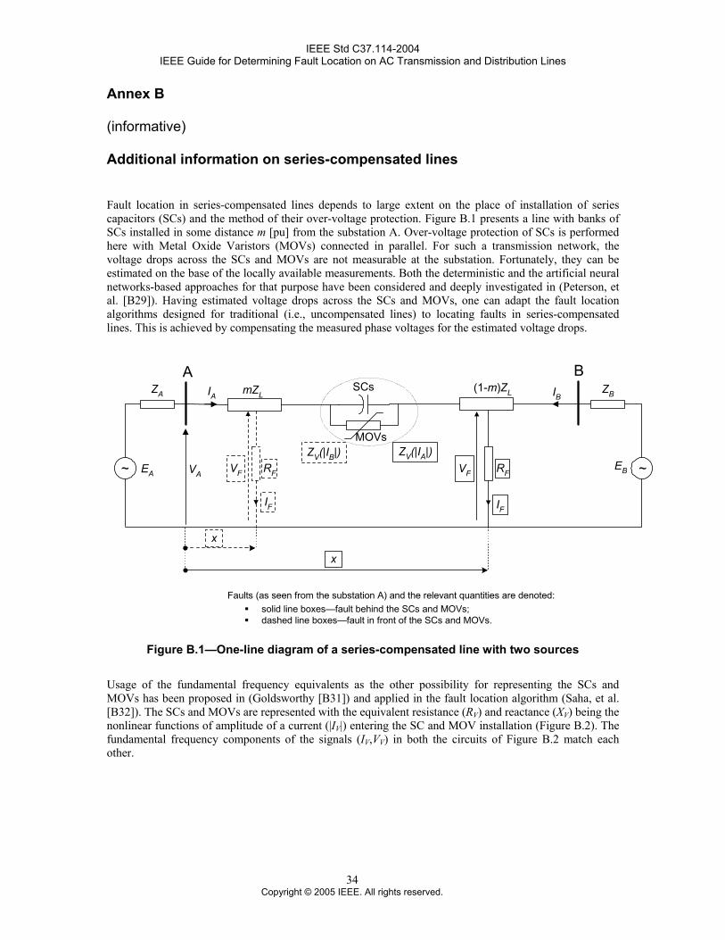
IEEE Std C37.114-2004 IEEE Guide for Determining Fault Location on AC Transmission and Distribution Lines
Annex B
(informative)
Additional information on series-compensated lines
Fault location in series-compensated lines depends to large extent on the place of installation of series capacitors (SCs) and the method of their over-voltage protection. Figure B.1 presents a line with banks of SCs installed in some distance m [pu] from the substation A. Over-voltage protection of SCs is performed here with Metal Oxide Varistors (MOVs) connected in parallel. For such a transmission network, the voltage drops across the SCs and MOVs are not measurable at the substation. Fortunately, they can be estimated on the base of the locally available measurements. Both the deterministic and the artificial neural networks-based approaches for that purpose have been considered and deeply investigated in (Peterson, et al. [B29]). Having estimated voltage drops across the SCs and MOVs, one can adapt the fault location algorithms designed for traditional (i.e., uncompensated lines) to locating faults in series-compensated lines. This is achieved by compensating the measured phase voltages for the estimated voltage drops.
EA
ZA
EB
ZB
BA
~ ~ZV(|IA|)
IA mZL
VA
(1-m)ZL
VF
IF
IB
ZV(|IB|)VF
IF
x
x
SCs
MOVs
RF RF
solid line boxes—fault behind the SCs and MOVs;dashed line boxes—fault in front of the SCs and MOVs.
Faults (as seen from the substation A) and the relevant quantities are denoted:
Figure B.1—One-line diagram of a series-compensated line with two sources
Usage of the fundamental frequency equivalents as the other possibility for representing the SCs and MOVs has been proposed in (Goldsworthy [B31]) and applied in the fault location algorithm (Saha, et al. [B32]). The SCs and MOVs are represented with the equivalent resistance (RV) and reactance (XV) being the nonlinear functions of amplitude of a current (|IV|) entering the SC and MOV installation (Figure B.2). The fundamental frequency components of the signals (IV,VV) in both the circuits of Figure B.2 match each other.
34 Copyright © 2005 IEEE. All rights reserved.
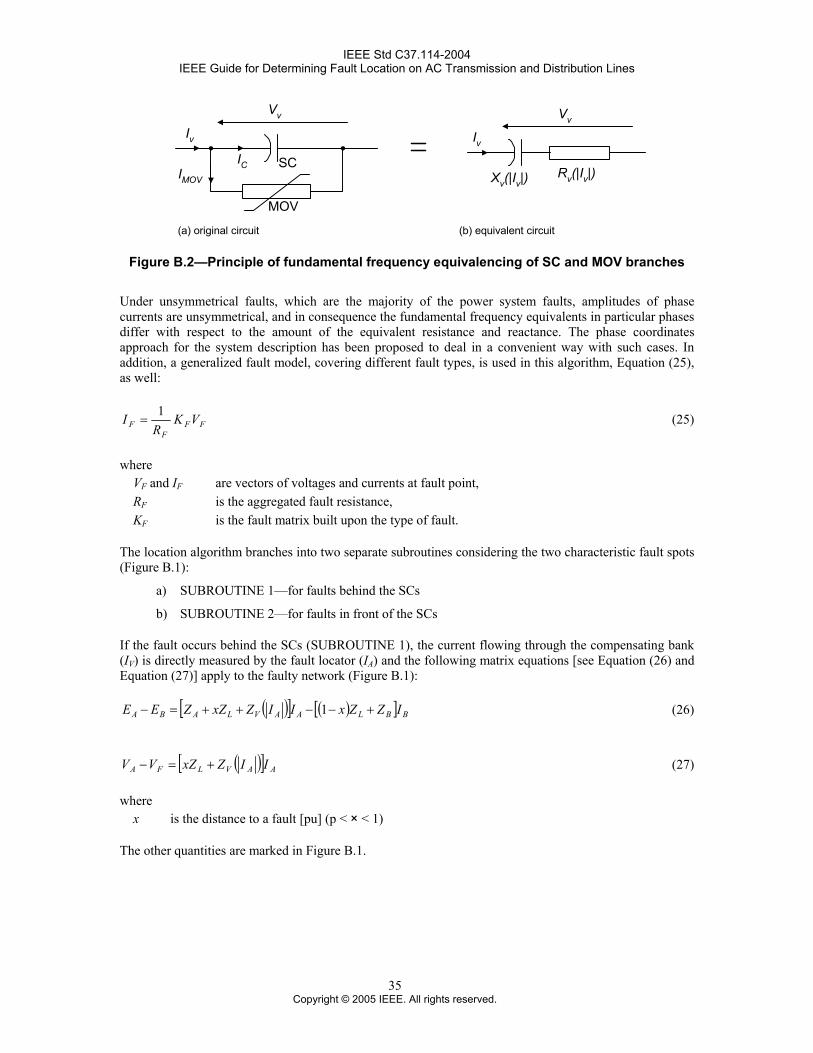
IEEE Std C37.114-2004 IEEE Guide for Determining Fault Location on AC Transmission and Distribution Lines
IMOV
Vv
Xv(|Iv|)Rv(|Iv|)
SC
MOV
Iv
Vv
IvIC
(a) original circuit (b) equivalent circuit
Figure B.2—Principle of fundamental frequency equivalencing of SC and MOV branches
Under unsymmetrical faults, which are the majority of the power system faults, amplitudes of phase currents are unsymmetrical, and in consequence the fundamental frequency equivalents in particular phases differ with respect to the amount of the equivalent resistance and reactance. The phase coordinates approach for the system description has been proposed to deal in a convenient way with such cases. In addition, a generalized fault model, covering different fault types, is used in this algorithm, Equation (25), as well:
FFF
F VKR
I 1= (25)
where VF and IF are vectors of voltages and currents at fault point, RF is the aggregated fault resistance, KF is the fault matrix built upon the type of fault.
The location algorithm branches into two separate subroutines considering the two characteristic fault spots (Figure B.1):
a) SUBROUTINE 1—for faults behind the SCs
b) SUBROUTINE 2—for faults in front of the SCs
If the fault occurs behind the SCs (SUBROUTINE 1), the current flowing through the compensating bank (IV) is directly measured by the fault locator (IA) and the following matrix equations [see Equation (26) and Equation (27)] apply to the faulty network (Figure B.1):
( )[ ] ( )[ ] BBLAAVLABA IZZxIIZxZ ZEE +−−++=− 1 (26)
( )[ ] AAVLFA IIZxZVV +=− (27)
where x is the distance to a fault [pu] (p < × < 1)
The other quantities are marked in Figure B.1.
35 Copyright © 2005 IEEE. All rights reserved.
IEEE Std C37.114-2004 IEEE Guide for Determining Fault Location on AC Transmission and Distribution Lines
For the pre-fault network (the subscript pre denotes the pre-fault values), the following, as seen in Equation (28), holds:
( )[ ] preABpreAVLABA IZIZZ ZEE __ +++=− (28)
The set of the above matrix equations is solved for x and , which yields the simple quadratic equation: FR
02 =−++ FRCBxAx (29)
where A, B, and C are the complex scalars determined with the system parameters and the local measurements
Resolving the above quadratic equation into the real and imaginary parts allows calculating the sought after fault distance (x).
On the other hand, in the case of a fault between the substation and the SCs (SUBROUTINE 2), the current flowing through the SCs and MOVs is not directly measured by the locator (IV = IB ≠ IA) and the following applies to the faulty network (Figure B.1):
( ) ( ) ( )[ ] BBBVLALABA IZIZZxIxZZEE ++−−+=− 1 (30)
( ) ALFA IxZVV =− (31)
where 0 < x < m
In consequence, one also obtains the quadratic equation as for the SUBPROCEDURE 1, but the iterative numerical solution is required because the coefficients depend on the unknown amplitudes of the phase currents from the remote Substation B.
The fault location algorithm has been implemented in one Swedish utility and is undergoing field tests on 400 kV series-compensated lines (Saha, et al. [B33]). Further extension of the algorithm for locating faults in series-compensated parallel lines is described in (Saha, et al. [B34]).
36 Copyright © 2005 IEEE. All rights reserved.