IEEE 13 Node Illustration

Radial Distribution Test Feeders

Distribution System Analysis Subcommittee Report

Abstract: Many computer programs are available forthe analysis of radial distribution feeders. In 1992 apaper was published [1] that presented the completedata for three four-wire wye and one three-wire deltaradial distribution test feeders. The purpose ofpublishing the data was to make available a commonset of data that could be used by program developersand users to verify the correctness of their solutions.

This paper presents an updated version of the same testfeeders along with a simple system that can be used totest three-phase transformer models.

Keywords: distribution system analysis, test systems,computer programs, transformer models

I. Introduction

In recent years many digital computer programs have beendeveloped for the analysis of unbalanced three-phase radialdistribution feeders. The programs use a wide variety ofiterative techniques and range from very simple with manysimplifying assumptions made for line and load models tovery sophisticated with little if any simplifyingassumptions. With so many different programs availablethere is a need for benchmark test feeders so that theresults of various programs can be compared.

This paper presents the complete data for three four-wirewye, one three-wire delta test feeders and a simple feederfor testing three-phase transformer models. Only the datafor the 13 node test feeder will be presented in this paper.The complete data and solutions for all of the test feederscan be downloaded from the Internet athttp://ewh.ieee.org/soc/pes/dsacom/testfeeders.html._______________________________________________The systems described in this paper were approved by the DistributionSystems Analysis Subcommittee during the 2000 PES Summer Meeting.The paper was written by W. H. Kersting, Professor of ElectricalEngineering at New Mexico State University.

II. Basic Data

The following data will be common for all systems:

Load Models:

Loads can be connected at a node (spot load) or assumedto be uniformly distributed along a line section (distributedload). Loads can be three-phase (balanced or unbalanced)or single-phase. Three-phase loads can be connected inwye or delta while single-phase loads can be connectedline-to-ground or line-to-line. All loads can be modeledas constant kW and kVAr (PQ), constant impedance (Z) orconstant current (I).Table 1 lists the codes that will be used to describe thevarious loads.

Table 1Load Model Codes

Code Connection ModelY-PQ Wye Constant kW and kVArY-I Wye Constant CurrentY-Z Wye Constant ImpedanceD-PQ Delta Constant kW and kVArD-I Delta Constant CurrentD-Z Delta Constant Impedance

Single-phase loads connected line-to-line will be assigneddelta connection codes regardless of whether the feeder isa four-wire wye or three-wire delta.

All of the load data will be specified in kW and kVAr orkW and power factor per phase. For constant current andconstant impedance loads the kW and kVAr should beconverted by assuming rated voltage (1.0 per-unit). Forwye connected loads, phases 1, 2 and 3 will be connecteda-g, b-g and c-g respectively and delta connected loadswill be connected a-b, b-c and c-a respectively. Only non-zero loads will be given in the various feeder load tables.All other loads are assumed to be zero.

Shunt Capacitors:

Shunt capacitor banks may be three-phase wye or deltaconnected and single-phase connected line-to-ground orline-to-line. The capacitors are modeled as constantsusceptance and specified at nameplate rated kVAr.

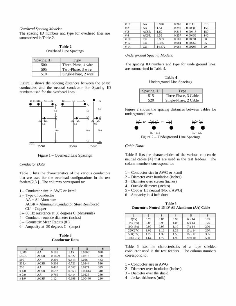
Overhead Spacing Models:The spacing ID numbers and type for overhead lines aresummarized in Table 2.

Table 2Overhead Line Spacings

Spacing ID Type 500 Three-Phase, 4 wire 505 Two-Phase, 3 wire 510 Single-Phase, 2 wire

Figure 1 shows the spacing distances between the phaseconductors and the neutral conductor for Spacing IDnumbers used for the overhead lines.

Figure 1 – Overhead Line Spacings

Conductor Data

Table 3 lists the characteristics of the various conductorsthat are used for the overhead configurations in the testfeeders[2,3 ]. The columns correspond to:

1 – Conductor size in AWG or kcmil2 – Type of conductor AA = All Aluminum ACSR = Aluminum Conductor Steel Reinforced CU = Copper3 – 60 Hz resistance at 50 degrees C (ohms/mile)4 – Conductor outside diameter (inches)5 – Geometric Mean Radius (ft.)6 – Ampacity at 50 degrees C (amps)

Table 3Conductor Data

1 2 3 4 5 61,000 AA 0.105 1.15 0.0368 698556.5 ACSR 0.1859 0.927 0.0313 730500 AA 0.206 0.813 0.026 483336.4 ACSR 0.306 0.721 0.0244 530250 AA 0.410 0.567 0.0171 329# 4/0 ACSR 0.592 0.563 0.00814 340# 2/0 AA 0.769 0.414 0.0125 230# 1/0 ACSR 1.12 0.398 0.00446 230

# 1/0 AA 0.970 0.368 0.0111 310# 2 AA 1.54 0.292 0.00883 156# 2 ACSR 1.69 0.316 0.00418 180# 4 ACSR 2.55 0.257 0.00452 140# 10 CU 5.903 0.102 0.00331 80# 12 CU 9.375 0.081 0.00262 75# 14 CU 14.872 0.064 0.00208 20

Underground Spacing Models:

The spacing ID numbers and type for underground linesare summarized in Table 4.

Table 4Underground Line Spacings

Spacing ID Type515 Three-Phase, 3 Cable520 Single-Phase, 2 Cable

Figure 2 shows the spacing distances between cables forunderground lines:

Figure 2 – Underground Line Spacings

Cable Data:

Table 5 lists the characteristics of the various concentricneutral cables [4] that are used in the test feeders. Thecolumn numbers correspond to:

1 – Conductor size in AWG or kcmil2 – Diameter over insulation (inches)3 – Diameter over screen (inches)4 – Outside diameter (inches)5 – Copper 1/3 neutral (No. x AWG)6 – Ampacity in 4 inch duct

Table 5Concentric Neutral 15 kV All Aluminum (AA) Cable

1 2 3 4 5 62(7x) 0.78 0.85 0.98 6 x 14 135

1/0(19x) 0.85 0.93 1.06 6 x 14 1752/0(19x) 0.90 0.97 1.10 7 x 14 200250(37x) 1.06 1.16 1.29 13 x 14 260500(37x) 1.29 1.39 1.56 16 x 12 385

1000(61x) 1.64 1.77 1.98 20 x 10 550

Table 6 lists the characteristics of a tape shieldedconductor used in the test feeders. The column numberscorrespond to:

1 – Conductor size in AWG2 – Diameter over insulation (inches)3 – Diameter over the shield4 – Jacket thickness (mils)

2.5 4.5

4.0

7.0

4.05.0

0.50.50.5

24.0 24.0 24.0

ID-500 ID-505 ID-510

6" 6"

ID - 515

1"

ID - 520

5 – Outside diameter (inches)6 – Ampacity in 4 inch duct (amps)

Table 6Tape Shielded 15 kV All Aluminum (AA) Cable

Tape Thickness = 5 mils

1 2 3 4 5 61/0 0.82 0.88 80 1.06 165

Configuration Codes:

Each test feeder will have a table of “ConfigurationCodes”. The configuration code is a unique numberassigned to describe the spacing model (Tables 2 and 4),the phasing (left to right) and the phase and neutralconductors used.

Line Segment Data:

Each test feeder will have a table of “Line Segment Data”.The data will consist of the node terminations of each linesegment (Node A and Node B), the length of the linesegment and a configuration code ( Config.). There is nosignificance in the order in which the data appears orwhether node A or node B is closer to the source.

Voltage Regulators:

Voltage regulators are assumed to be “step-type” and canbe connected in the substation and/or to a specified linesegment. The regulators can be three-phase or single-phase. Tap positions will be determined by thecompensator circuit settings described by:

1. Voltage Level – desired voltage (on a 120 volt base)to be held at the regulating point.

2. Bandwidth – the voltage level tolerance usuallyassumed to be 2 volts.

3. Compensator – resistance (R) and reactance (X)settings – the equivalent resistance and reactancebetween the regulator and the regulating pointcalibrated in volts.

4. PT Ratio – turns ratio of the potential transformerfeeding the compensator circuit.

5. CT Rating – the current rating on the primary of thecurrent transformer feeding the compensator circuit.

III. The Test Feeders

The data for the feeders is so extensive that only the datafor the 13 node feeder will be given in this paper. Data forall of the test feeders can be downloaded from:http://ewh.ieee.org/soc/pes/dsacom/testfeeders.html.The data is in a spreadsheet format. In addition to the dataa solution for each of the feeders can be downloaded. Thesolution consists of:1. Listing of the per mile phase impedance and

admittance matrices for each of the configurations

used in the feeder. The impedance matrix assumes aresistivity of 100 Ohm-meters and the admittancematrix assumes a relative permittivity of 2.3.

2. Radial Flow Summary –a summary of the systeminput, total load, total losses and total shunt capacitorsby phase and total three-phase.

3. Voltage Profile – voltage magnitudes and angles byphase at each node. Voltage magnitudes are given inper-unit.

4. Voltage Regulator Data – for each regulator in thesystem a summary of the settings and the final tapsettings.

5. Radial Power Flow – complete node data includingline flows in amps and degrees by phase. Line powerlosses by phase and total three-phase are also given.

The IEEE 13 Node Test Feeder

This feeder is very small and yet displays some veryinteresting characteristics.

1. Short and relatively highly loaded for a 4.16 kV feeder2. One substation voltage regulator consisting of three

single-phase units connected in wye3. Overhead and underground lines with variety of

phasing4. Shunt capacitor banks5. In-line transformer6. Unbalanced spot and distributed loads

For a small feeder this will provide a good test for the mostcommon features of distribution analysis software.

The complete data for this system is given below toillustrate the form of the data for all of the test feeders.

One Line Diagram

646 645 632 633 634

650

692 675611 684

652

671

680Underground Line Configuration Data:

Config. Phasing Cable Neutral SpaceID

606 A B C N 250,000 AA, CN None 515

607 A N 1/0 AA, TS 1/0 Cu 520

Overhead Line Configuration Data:

Config. Phasing Phase Neutral Spacing

ACSR ACSR ID

601 B A C N 556,500 26/7 4/0 6/1 500

602 C A B N 4/0 6/1 4/0 6/1 500

603 C B N 1/0 1/0 505

604 A C N 1/0 1/0 505

605 C N 1/0 1/0 510

Line Segment Data:

Node A Node B Length(ft.) Config.

632 645 500 603

632 633 500 602

633 634 0 XFM-1

645 646 300 603

650 632 2000 601

684 652 800 607

632 671 2000 601

671 684 300 604

671 680 1000 601

671 692 0 Switch

684 611 300 605

692 675 500 606

Capacitor Data:

Node Ph-A Ph-B Ph-C

kVAr kVAr kVAr

675 200 200 200

611 100

Total 200 200 300

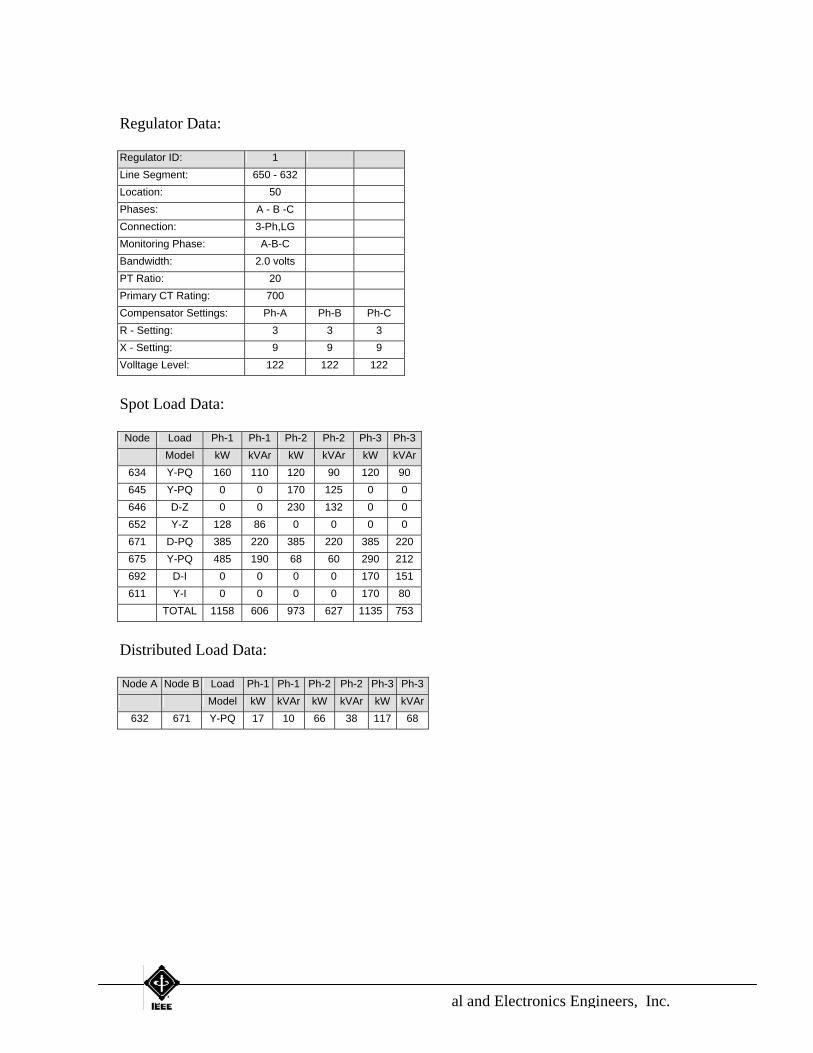
Regulator Data:

Regulator ID: 1

Line Segment: 650 - 632

Location: 650

Phases: A - B -C

Connection: 3-Ph,LG

Monitoring Phase: A-B-C

Bandwidth: 2.0 volts

PT Ratio: 20

Primary CT Rating: 700

Compensator Settings: Ph-A Ph-B Ph-C

R - Setting: 3 3 3

X - Setting: 9 9 9

Volltage Level: 122 122 122

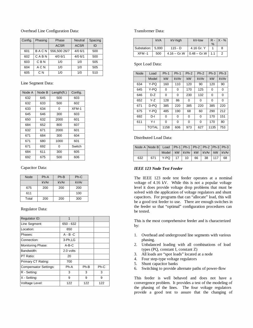
Transformer Data:

kVA kV-high kV-low R -%

X - %

Substation: 5,000 115 - D 4.16 Gr. Y 1 8

XFM -1 500 4.16 – Gr.W 0.48 – Gr.W 1.1 2

Spot Load Data:

Node Load Ph-1 Ph-1 Ph-2 Ph-2 Ph-3 Ph-3

Model kW kVAr kW kVAr kW kVAr

634 Y-PQ 160 110 120 90 120 90

645 Y-PQ 0 0 170 125 0 0

646 D-Z 0 0 230 132 0 0

652 Y-Z 128 86 0 0 0 0

671 D-PQ 385 220 385 220 385 220

675 Y-PQ 485 190 68 60 290 212

692 D-I 0 0 0 0 170 151

611 Y-I 0 0 0 0 170 80

TOTAL 1158 606 973 627 1135 753

Distributed Load Data:

Node A Node B Load Ph-1 Ph-1 Ph-2 Ph-2 Ph-3 Ph-3

Model kW kVAr kW kVAr kW kVAr

632 671 Y-PQ 17 10 66 38 117 68

IEEE 123 Node Test Feeder

The IEEE 123 node test feeder operates at a nominalvoltage of 4.16 kV. While this is not a popular voltagelevel it does provide voltage drop problems that must besolved with the application of voltage regulators and shuntcapacitors. For programs that can “allocate” load, this willbe a good test feeder to use. There are enough switches inthe feeder so that “optimal” configuration procedures canbe tested.

This is the most comprehensive feeder and is characterizedby:

1. Overhead and underground line segments with variousphasing.

2. Unbalanced loading with all combinations of loadtypes (PQ, constant I, constant Z)

3. All loads are “spot loads” located at a node4. Four step-type voltage regulators5. Shunt capacitor banks6. Switching to provide alternate paths of power-flow

This feeder is well behaved and does not have aconvergence problem. It provides a test of the modeling ofthe phasing of the lines. The four voltage regulatorsprovide a good test to assure that the changing of

individual regulator taps is coordinated with the otherregulators.


This feeder is an actual feeder located in Arizona. Thefeeder’s nominal voltage is 24.9 kV. It is characterized by:

1. Very long and lightly loaded2. Two in-line regulators required to maintain a good

voltage profile3. An in-line transformer reducing the voltage to 4.16 kV

for a short section of the feeder4. Unbalanced loading with both “spot” and

“distributed” loads. Distributed loads are assumed tobe connected at the center of the line segment

5. Shunt capacitors

Because of the length of the feeder and the unbalancedloading it can have a convergence problem.


This feeder is an actual feeder located in California. Thecharacteristics of the feeder are:

1. Three-wire delta operating at a nominal voltage of4.8 kV

2. All line segments are underground3. Substation voltage regulator consisting of two single-

phase units connected in open delta4. All loads are “spot” loads and consist of constant PQ,

constant current and constant impedance5. The loading is very unbalanced

Although there are very few three-wire delta systems inuse, there is a need to test software to assure that it canhandle this type of feeder.

The IEEE Four Node Test Feeder

This feeder was not part of the original set of test systemspublished in 1992. The primary purpose of this test feederis to provide a simple system for the testing of all possiblethree-phase transformer connections. Characteristics ofthe feeder are:

1. Two line segments with a three-phase transformerbank connected between the two segments

2. Data is specified for “closed” three-phase transformerconnections and for two transformer “open”connections

3. Transformer data is specified for step-up and step-down testing. The primary voltage is always 12.47kV while the secondary voltage can be either 4.16 kVor 24.9 kV.

4. Data is specified for balanced and unbalanced loadingat the most remote node

Test results for this feeder include the followingtransformer connections for step-down and step-upoperations and for balanced and unbalanced loading.

1. Grounded Wye – Grounded Wye2. Grounded Wye – Delta3. Ungrounded Wye – Delta4. Delta – Grounded Wye5. Delta – Delta6. Open Wye – Open Delta

IV. Summary

Data for five different test feeders has been developed.Data appearing in this paper are “common” to all of thefeeders. The total data for the 13 node test feeder isincluded to illustrate the form of the data for the other testfeeders. The data and one-line diagrams for the other testfeeders are too extensive to be included in the paper. Thedata for all five test feeders are in spreadsheet format andcan be downloaded from the Web at:

http://ewh.ieee.org/soc/pes/dsacom/testfeeders.html

The test feeders have been studied using the RadialDistribution Analysis Package of WH Power Consultants,Las Cruces, New Mexico and/or Windmil developed byMilsoft Integrated Solutions, Abilene, Texas. The resultsof these tests are included with the data for each feeder.

Software developers are encouraged to test their softwareusing these test feeders and to publish the results. Thehope is that in time there will be agreement on the resultsin the same way that there is agreement on the various testsystems used by network power-flow programs.

V. References:

1. IEEE Distribution Planning Working Group Report,“Radial distribution test feeders”, IEEE Transactioinson Power Systems,, August 1991, Volume 6, Number3, pp 975-985.

2. J.D. Glover and M. Sarma, “Power system analysisand design”, 2nd Edition, PWS Publishing Company,Boston, MA, 1994.

3. “Overhead conductor manual”, Southwire Company,Carrollton, GA, 1994.

4. “Product data”, Section 2, Sheets 10 and 30., TheOkonite Company, www.okonite.com

IEEE POWER ENGINEERING SOCIETY Power System Analysis, Computing and Economics Committee

Subcommittee Chairs

Chair MARTIN L. BAUGHMAN Professor Emeritus The University of Texas at Austin 5703 Painted Valley Drive Austin, TX 78759 Vox: 512-345-8255 Fax: 512-345-9880 [email protected]

Vice Chair CHEN-CHING LIU Dept. of Electrical Eng. University of Washington Box 352500 Seattle, WA 98195 Vox: 206-543-2198 Fax: 206-543-3842 [email protected]

Secretary ROGER C. DUGAN Sr. Consultant Electrotek Concepts, Inc. 408 N Cedar Bluff Rd Knoxville, TN 37923 Vox: 865-470-9222 Fax: 865-470-9223 [email protected] Computer & Analytical Methods

EDWIN LIU, Chair Nexant, Inc. 101, 2nd street, 11F San Francisco CA 94105 Vox: 415-369-1088 Fax: 415-369-0894 [email protected] Distribution Systems Analysis SANDOVAL CARNEIRO, JR, Chair Dept. of Electrical Engineering Federal Univ. of Rio de Janeiro Rio de Janeiro, RJ, Brazil Vox: 55-21-25628025 Fax: 55-21-25628628 [email protected] Intelligent System Applications DAGMAR NIEBUR, Chair Department of ECE Drexel University 3141 Chestnut Street Philadelphia, PA 19104 Vox: (215) 895 6749 Fax: (215) 895 1695 [email protected] Reliability, Risk & Probability Applications JAMES D. MCCALLEY, Chair Iowa State University Room 2210 Coover Hall Ames, Iowa 50011 Vox: 515-294-4844 Fax: 515-294-4263 [email protected] Systems Economics ROSS BALDICK, Chair ECE Dept. , ENS 502 The University of Texas at Austin Austin, TX 78712 Vox: 512-471-5879 Fax: 512-471-5532 [email protected] Past Chair JOANN V. STARON Nexant Inc/ PCA 1921 S. Alma School Road Suite 207 Mesa, AZ 85210 Vox: 480-345-7600 Fax: 480-345-7601 [email protected]

Distribution System Analysis Subcommittee


The Institute of Electrical and Electronics Engineers, Inc.


646 645 632 633 634

650

692 675611 684

652

671

680


Overhead Line Configuration Data: Config. Phasing Phase Neutral Spacing

ACSR ACSR ID 601 B A C N 556,500 26/7 4/0 6/1 500 602 C A B N 4/0 6/1 4/0 6/1 500 603 C B N 1/0 1/0 505 604 A C N 1/0 1/0 505 605 C N 1/0 1/0 510

Underground Line Configuration Data: Config. Phasing Cable Neutral Space

ID 606 A B C N 250,000 AA, CN None 515 607 A N 1/0 AA, TS 1/0 Cu 520

Line Segment Data: Node A Node B Length(ft.) Config.

632 645 500 603 632 633 500 602 633 634 0 XFM-1 645 646 300 603 650 632 2000 601 684 652 800 607 632 671 2000 601 671 684 300 604 671 680 1000 601 671 692 0 Switch 684 611 300 605 692 675 500 606

Transformer Data:

kVA kV-high kV-low R - %

X - %

Substation: 5,000 115 - D 4.16 Gr. Y 1 8 XFM -1 500 4.16 – Gr.W 0.48 – Gr.W 1.1 2

Capacitor Data:

Node Ph-A Ph-B Ph-C kVAr kVAr kVAr

675 200 200 200 611 100

Total 200 200 300


Regulator Data: Regulator ID: 1 Line Segment: 650 - 632 Location: 50 Phases: A - B -C Connection: 3-Ph,LG Monitoring Phase: A-B-C Bandwidth: 2.0 volts PT Ratio: 20 Primary CT Rating: 700 Compensator Settings: Ph-A Ph-B Ph-C R - Setting: 3 3 3 X - Setting: 9 9 9 Volltage Level: 122 122 122

Spot Load Data: Node Load Ph-1 Ph-1 Ph-2 Ph-2 Ph-3 Ph-3

Model kW kVAr kW kVAr kW kVAr634 Y-PQ 160 110 120 90 120 90 645 Y-PQ 0 0 170 125 0 0 646 D-Z 0 0 230 132 0 0 652 Y-Z 128 86 0 0 0 0 671 D-PQ 385 220 385 220 385 220 675 Y-PQ 485 190 68 60 290 212 692 D-I 0 0 0 0 170 151 611 Y-I 0 0 0 0 170 80

TOTAL 1158 606 973 627 1135 753

Distributed Load Data: Node A Node B Load Ph-1 Ph-1 Ph-2 Ph-2 Ph-3 Ph-3

Model kW kVAr kW kVAr kW kVAr632 671 Y-PQ 17 10 66 38 117 68


IEEE 13 NODE TEST FEEDER Impedances

Configuration 601: Z (R +jX) in ohms per mile 0.3465 1.0179 0.1560 0.5017 0.1580 0.4236 0.3375 1.0478 0.1535 0.3849 0.3414 1.0348 B in micro Siemens per mile 6.2998 -1.9958 -1.2595 5.9597 -0.7417 5.6386 Configuration 602: Z (R +jX) in ohms per mile 0.7526 1.1814 0.1580 0.4236 0.1560 0.5017 0.7475 1.1983 0.1535 0.3849 0.7436 1.2112 B in micro Siemens per mile 5.6990 -1.0817 -1.6905 5.1795 -0.6588 5.4246 Configuration 603: Z (R +jX) in ohms per mile 0.0000 0.0000 0.0000 0.0000 0.0000 0.0000 1.3294 1.3471 0.2066 0.4591 1.3238 1.3569 B in micro Siemens per mile 0.0000 0.0000 0.0000 4.7097 -0.8999 4.6658 Configuration 604: Z (R +jX) in ohms per mile 1.3238 1.3569 0.0000 0.0000 0.2066 0.4591 0.0000 0.0000 0.0000 0.0000 1.3294 1.3471 B in micro Siemens per mile 4.6658 0.0000 -0.8999 0.0000 0.0000 4.7097


Configuration 605: Z (R +jX) in ohms per mile 0.0000 0.0000 0.0000 0.0000 0.0000 0.0000 0.0000 0.0000 0.0000 0.0000 1.3292 1.3475 B in micro Siemens per mile 0.0000 0.0000 0.0000 0.0000 0.0000 4.5193 Configuration 606: Z (R +jX) in ohms per mile 0.7982 0.4463 0.3192 0.0328 0.2849 -0.0143 0.7891 0.4041 0.3192 0.0328 0.7982 0.4463 B in micro Siemens per mile 96.8897 0.0000 0.0000 96.8897 0.0000 96.8897 Configuration 607: Z (R +jX) in ohms per mile 1.3425 0.5124 0.0000 0.0000 0.0000 0.0000 0.0000 0.0000 0.0000 0.0000 0.0000 0.0000 B in micro Siemens per mile 88.9912 0.0000 0.0000 0.0000 0.0000 0.0000


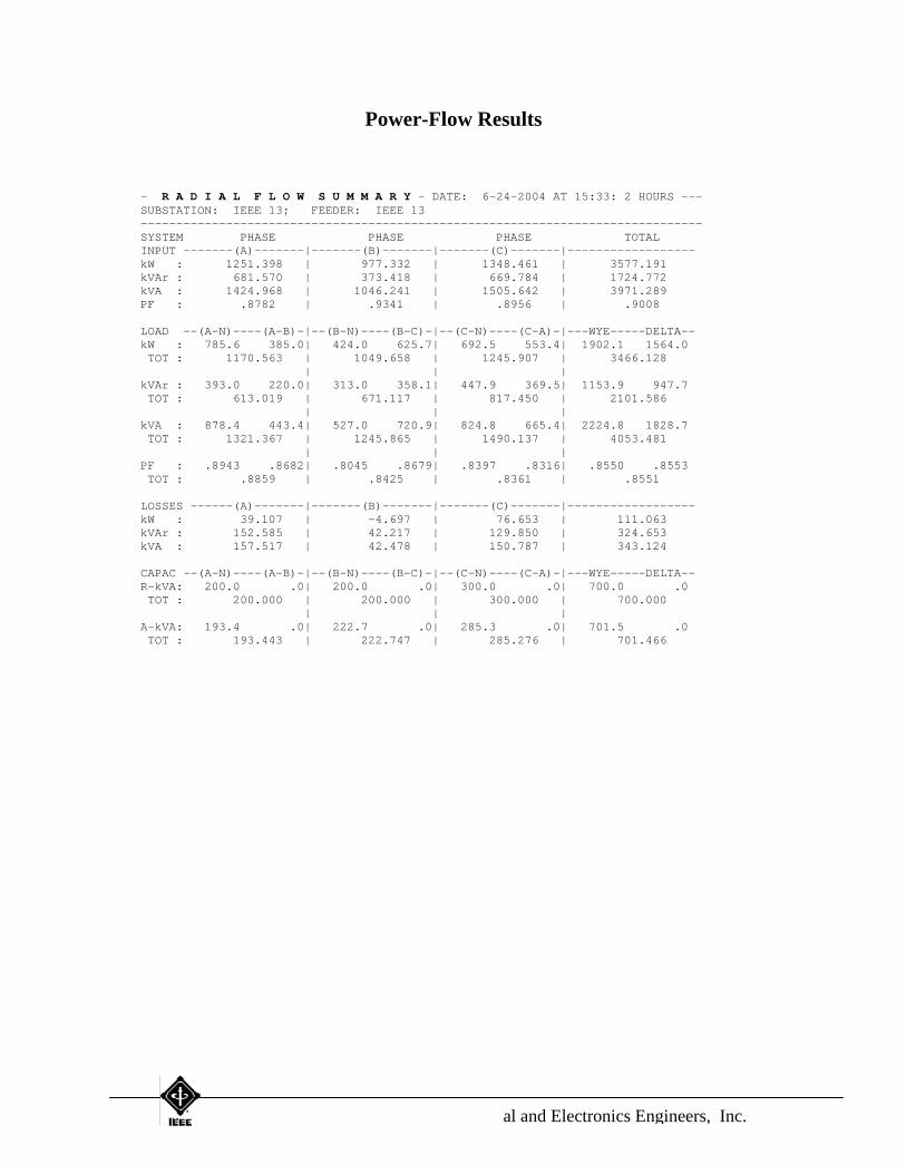
Power-Flow Results - R A D I A L F L O W S U M M A R Y - DATE: 6-24-2004 AT 15:33: 2 HOURS --- SUBSTATION: IEEE 13; FEEDER: IEEE 13 ------------------------------------------------------------------------------- SYSTEM PHASE PHASE PHASE TOTAL INPUT -------(A)-------|-------(B)-------|-------(C)-------|------------------ kW : 1251.398 | 977.332 | 1348.461 | 3577.191 kVAr : 681.570 | 373.418 | 669.784 | 1724.772 kVA : 1424.968 | 1046.241 | 1505.642 | 3971.289 PF : .8782 | .9341 | .8956 | .9008 LOAD --(A-N)----(A-B)-|--(B-N)----(B-C)-|--(C-N)----(C-A)-|---WYE-----DELTA-- kW : 785.6 385.0| 424.0 625.7| 692.5 553.4| 1902.1 1564.0 TOT : 1170.563 | 1049.658 | 1245.907 | 3466.128 | | | kVAr : 393.0 220.0| 313.0 358.1| 447.9 369.5| 1153.9 947.7 TOT : 613.019 | 671.117 | 817.450 | 2101.586 | | | kVA : 878.4 443.4| 527.0 720.9| 824.8 665.4| 2224.8 1828.7 TOT : 1321.367 | 1245.865 | 1490.137 | 4053.481 | | | PF : .8943 .8682| .8045 .8679| .8397 .8316| .8550 .8553 TOT : .8859 | .8425 | .8361 | .8551 LOSSES ------(A)-------|-------(B)-------|-------(C)-------|------------------ kW : 39.107 | -4.697 | 76.653 | 111.063 kVAr : 152.585 | 42.217 | 129.850 | 324.653 kVA : 157.517 | 42.478 | 150.787 | 343.124 CAPAC --(A-N)----(A-B)-|--(B-N)----(B-C)-|--(C-N)----(C-A)-|---WYE-----DELTA-- R-kVA: 200.0 .0| 200.0 .0| 300.0 .0| 700.0 .0 TOT : 200.000 | 200.000 | 300.000 | 700.000 | | | A-kVA: 193.4 .0| 222.7 .0| 285.3 .0| 701.5 .0 TOT : 193.443 | 222.747 | 285.276 | 701.466


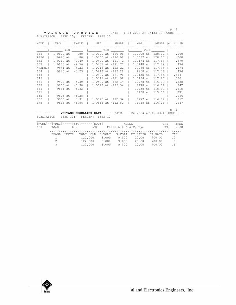
p 1 --- V O L T A G E P R O F I L E ---- DATE: 6-24-2004 AT 15:33:12 HOURS ---- SUBSTATION: IEEE 13; FEEDER: IEEE 13 ------------------------------------------------------------------------------- NODE | MAG ANGLE | MAG ANGLE | MAG ANGLE |mi.to SR ------------------------------------------------------------------------------- ______|_______ A-N ______ |_______ B-N _______ |_______ C-N _______ | 650 | 1.0000 at .00 | 1.0000 at -120.00 | 1.0000 at 120.00 | .000 RG60 | 1.0625 at .00 | 1.0500 at -120.00 | 1.0687 at 120.00 | .000 632 | 1.0210 at -2.49 | 1.0420 at -121.72 | 1.0174 at 117.83 | .379 633 | 1.0180 at -2.56 | 1.0401 at -121.77 | 1.0148 at 117.82 | .474 XFXFM1| .9941 at -3.23 | 1.0218 at -122.22 | .9960 at 117.35 | .474 634 | .9940 at -3.23 | 1.0218 at -122.22 | .9960 at 117.34 | .474 645 | | 1.0329 at -121.90 | 1.0155 at 117.86 | .474 646 | | 1.0311 at -121.98 | 1.0134 at 117.90 | .530 671 | .9900 at -5.30 | 1.0529 at -122.34 | .9778 at 116.02 | .758 680 | .9900 at -5.30 | 1.0529 at -122.34 | .9778 at 116.02 | .947 684 | .9881 at -5.32 | | .9758 at 115.92 | .815 611 | | | .9738 at 115.78 | .871 652 | .9825 at -5.25 | | | .966 692 | .9900 at -5.31 | 1.0529 at -122.34 | .9777 at 116.02 | .852 675 | .9835 at -5.56 | 1.0553 at -122.52 | .9758 at 116.03 | .947 p 1 ----------- VOLTAGE REGULATOR DATA ---- DATE: 6-24-2004 AT 15:33:16 HOURS -- SUBSTATION: IEEE 13; FEEDER: IEEE 13 _______________________________________________________________________________ [NODE]--[VREG]-----[SEG]------[NODE] MODEL OPT BNDW 650 RG60 632 632 Phase A & B & C, Wye RX 2.00 ........................................................................ PHASE LDCTR VOLT HOLD R-VOLT X-VOLT PT RATIO CT RATE TAP 1 122.000 3.000 9.000 20.00 700.00 10 2 122.000 3.000 9.000 20.00 700.00 8 3 122.000 3.000 9.000 20.00 700.00 11


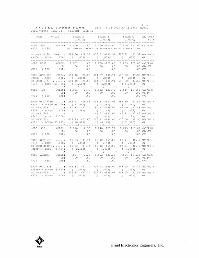
p 1 - R A D I A L P O W E R F L O W --- DATE: 6-24-2004 AT 15:33:27 HOURS --- SUBSTATION: IEEE 13; FEEDER: IEEE 13 ------------------------------------------------------------------------------- NODE VALUE PHASE A PHASE B PHASE C UNT O/L< (LINE A) (LINE B) (LINE C) 60.% ---------------------*--------A-------*-------B-------*-------C-------*-------- NODE: 650 VOLTS: 1.000 .00 1.000 -120.00 1.000 120.00 MAG/ANG kVll 4.160 NO LOAD OR CAPACITOR REPRESENTED AT SOURCE NODE TO NODE RG60 <VRG>..: 593.30 -28.58 435.61 -140.91 626.92 93.59 AMP/DG < <RG60 > LOSS= .000: ( .000) ( .000) ( .000) kW ---------------------*--------A-------*-------B-------*-------C-------*-------- NODE: RG60 VOLTS: 1.062 .00 1.050 -120.00 1.069 120.00 MAG/ANG -LD: .00 .00 .00 .00 .00 .00 kW/kVR kVll 4.160 CAP: .00 .00 .00 kVR FROM NODE 650 <VRG>: 558.40 -28.58 414.87 -140.91 586.60 93.59 AMP/DG < <RG60 > LOSS= .000: ( .000) ( .000) ( .000) kW TO NODE 632 .......: 558.40 -28.58 414.87 -140.91 586.60 93.59 AMP/DG < <632 > LOSS= 59.716: ( 21.517) ( -3.252) ( 41.451) kW ---------------------*--------A-------*-------B-------*-------C-------*-------- NODE: 632 VOLTS: 1.021 -2.49 1.042 -121.72 1.017 117.83 MAG/ANG -LD: .00 .00 .00 .00 .00 .00 kW/kVR kVll 4.160 CAP: .00 .00 .00 kVR FROM NODE RG60 .....: 558.41 -28.58 414.87 -140.91 586.60 93.59 AMP/DG < <632 > LOSS= 59.716: ( 21.517) ( -3.252) ( 41.451) kW TO NODE 633 .......: 81.33 -37.74 61.12 -159.09 62.70 80.48 AMP/DG <633 > LOSS= .808: ( .354) ( .148) ( .306) kW TO NODE 645 .......: 143.02 -142.66 65.21 57.83 AMP/DG < <645 > LOSS= 2.760: ( 2.540) ( .220) kW TO NODE 671 .......: 478.29 -27.03 215.12 -134.66 475.50 99.90 AMP/DG < <671 > LOSS= 35.897: ( 10.484) ( -6.169) ( 31.582) kW ---------------------*--------A-------*-------B-------*-------C-------*-------- NODE: 633 VOLTS: 1.018 -2.56 1.040 -121.77 1.015 117.82 MAG/ANG -LD: .00 .00 .00 .00 .00 .00 kW/kVR kVll 4.160 CAP: .00 .00 .00 kVR FROM NODE 632 .....: 81.33 -37.74 61.12 -159.09 62.71 80.47 AMP/DG <633 > LOSS= .808: ( .354) ( .148) ( .306) kW TO NODE XFXFM1.......: 81.33 -37.74 61.12 -159.09 62.71 80.47 AMP/DG < <XFXFM1> LOSS= 5.427: ( 2.513) ( 1.420) ( 1.494) kW ---------------------*--------A-------*-------B-------*-------C-------*-------- NODE: XFXFM1 VOLTS: .994 -3.23 1.022 -122.22 .996 117.35 MAG/ANG -LD: .00 .00 .00 .00 .00 .00 kW/kVR kVll .480 CAP: .00 .00 .00 kVR FROM NODE 633 .....: 704.83 -37.74 529.73 -159.09 543.45 80.47 AMP/DG < <XFXFM1> LOSS= 5.427: ( 2.513) ( 1.420) ( 1.494) kW TO NODE 634 .......: 704.83 -37.74 529.73 -159.09 543.45 80.47 AMP/DG < <634 > LOSS= .000: ( .000) ( .000) ( .000) kW


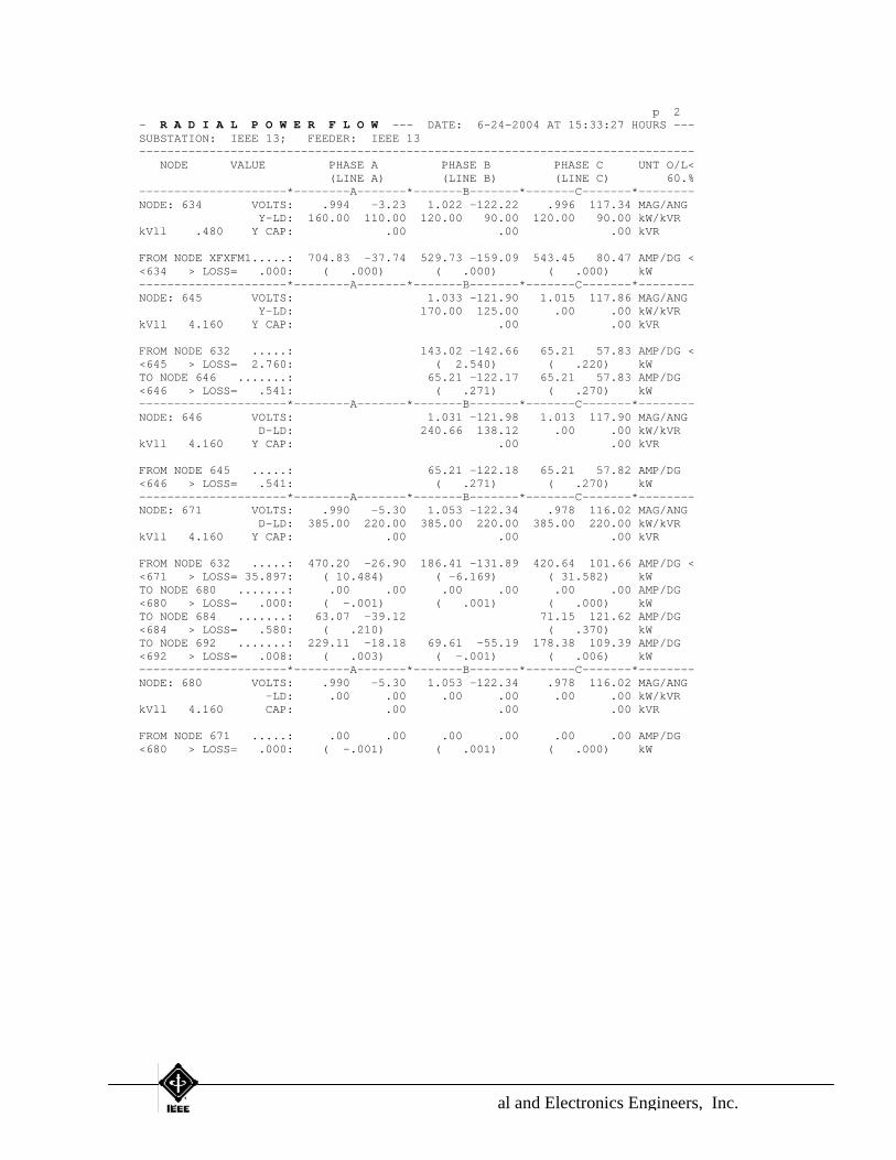
p 2 - R A D I A L P O W E R F L O W --- DATE: 6-24-2004 AT 15:33:27 HOURS --- SUBSTATION: IEEE 13; FEEDER: IEEE 13 ------------------------------------------------------------------------------- NODE VALUE PHASE A PHASE B PHASE C UNT O/L< (LINE A) (LINE B) (LINE C) 60.% ---------------------*--------A-------*-------B-------*-------C-------*-------- NODE: 634 VOLTS: .994 -3.23 1.022 -122.22 .996 117.34 MAG/ANG Y-LD: 160.00 110.00 120.00 90.00 120.00 90.00 kW/kVR kVll .480 Y CAP: .00 .00 .00 kVR FROM NODE XFXFM1.....: 704.83 -37.74 529.73 -159.09 543.45 80.47 AMP/DG < <634 > LOSS= .000: ( .000) ( .000) ( .000) kW ---------------------*--------A-------*-------B-------*-------C-------*-------- NODE: 645 VOLTS: 1.033 -121.90 1.015 117.86 MAG/ANG Y-LD: 170.00 125.00 .00 .00 kW/kVR kVll 4.160 Y CAP: .00 .00 kVR FROM NODE 632 .....: 143.02 -142.66 65.21 57.83 AMP/DG < <645 > LOSS= 2.760: ( 2.540) ( .220) kW TO NODE 646 .......: 65.21 -122.17 65.21 57.83 AMP/DG <646 > LOSS= .541: ( .271) ( .270) kW ---------------------*--------A-------*-------B-------*-------C-------*-------- NODE: 646 VOLTS: 1.031 -121.98 1.013 117.90 MAG/ANG D-LD: 240.66 138.12 .00 .00 kW/kVR kVll 4.160 Y CAP: .00 .00 kVR FROM NODE 645 .....: 65.21 -122.18 65.21 57.82 AMP/DG <646 > LOSS= .541: ( .271) ( .270) kW ---------------------*--------A-------*-------B-------*-------C-------*-------- NODE: 671 VOLTS: .990 -5.30 1.053 -122.34 .978 116.02 MAG/ANG D-LD: 385.00 220.00 385.00 220.00 385.00 220.00 kW/kVR kVll 4.160 Y CAP: .00 .00 .00 kVR FROM NODE 632 .....: 470.20 -26.90 186.41 -131.89 420.64 101.66 AMP/DG < <671 > LOSS= 35.897: ( 10.484) ( -6.169) ( 31.582) kW TO NODE 680 .......: .00 .00 .00 .00 .00 .00 AMP/DG <680 > LOSS= .000: ( -.001) ( .001) ( .000) kW TO NODE 684 .......: 63.07 -39.12 71.15 121.62 AMP/DG <684 > LOSS= .580: ( .210) ( .370) kW TO NODE 692 .......: 229.11 -18.18 69.61 -55.19 178.38 109.39 AMP/DG <692 > LOSS= .008: ( .003) ( -.001) ( .006) kW ---------------------*--------A-------*-------B-------*-------C-------*-------- NODE: 680 VOLTS: .990 -5.30 1.053 -122.34 .978 116.02 MAG/ANG -LD: .00 .00 .00 .00 .00 .00 kW/kVR kVll 4.160 CAP: .00 .00 .00 kVR FROM NODE 671 .....: .00 .00 .00 .00 .00 .00 AMP/DG <680 > LOSS= .000: ( -.001) ( .001) ( .000) kW


p 3 - R A D I A L P O W E R F L O W --- DATE: 6-24-2004 AT 15:33:27 HOURS --- SUBSTATION: IEEE 13; FEEDER: IEEE 13 ------------------------------------------------------------------------------- NODE VALUE PHASE A PHASE B PHASE C UNT O/L< (LINE A) (LINE B) (LINE C) 60.% ---------------------*--------A-------*-------B-------*-------C-------*-------- NODE: 684 VOLTS: .988 -5.32 .976 115.92 MAG/ANG -LD: .00 .00 .00 .00 kW/kVR kVll 4.160 CAP: .00 .00 kVR FROM NODE 671 .....: 63.07 -39.12 71.15 121.61 AMP/DG <684 > LOSS= .580: ( .210) ( .370) kW TO NODE 611 .......: 71.15 121.61 AMP/DG <611 > LOSS= .382: ( .382) kW TO NODE 652 .......: 63.07 -39.12 AMP/DG <652 > LOSS= .808: ( .808) kW ---------------------*--------A-------*-------B-------*-------C-------*-------- NODE: 611 VOLTS: .974 115.78 MAG/ANG Y-LD: 165.54 77.90 kW/kVR kVLL 4.160 Y CAP: 94.82 kVR FROM NODE 684 .....: 71.15 121.61 AMP/DG <611 > LOSS= .382: ( .382) kW ---------------------*--------A-------*-------B-------*-------C-------*-------- NODE: 652 VOLTS: .983 -5.25 MAG/ANG Y-LD: 123.56 83.02 kW/kVR kVll 4.160 Y CAP: .00 kVR FROM NODE 684 .....: 63.08 -39.15 AMP/DG <652 > LOSS= .808: ( .808) kW ---------------------*--------A-------*-------B-------*-------C-------*-------- NODE: 692 VOLTS: .990 -5.31 1.053 -122.34 .978 116.02 MAG/ANG D-LD: .00 .00 .00 .00 168.37 149.55 kW/kVR kVll 4.160 Y CAP: .00 .00 .00 kVR FROM NODE 671 .....: 229.11 -18.18 69.61 -55.19 178.38 109.39 AMP/DG <692 > LOSS= .008: ( .003) ( -.001) ( .006) kW TO NODE 675 .......: 205.33 -5.15 69.61 -55.19 124.07 111.79 AMP/DG < <675 > LOSS= 4.136: ( 3.218) ( .345) ( .573) kW ---------------------*--------A-------*-------B-------*-------C-------*-------- NODE: 675 VOLTS: .983 -5.56 1.055 -122.52 .976 116.03 MAG/ANG Y-LD: 485.00 190.00 68.00 60.00 290.00 212.00 kW/kVR kVll 4.160 Y CAP: 193.44 222.75 190.45 kVR FROM NODE 692 .....: 205.33 -5.15 69.59 -55.20 124.07 111.78 AMP/DG < <675 > LOSS= 4.136: ( 3.218) ( .345) ( .573) kW


Documents

IEEE 13 Node Illustration