Embed Size (px)
Citation preview

We
Loo, qt
IMPLICATIONS OF P-DELTA ANALYSIS
AND LRFD OF GABLE FRAMES
by
Eric J. Wishart
Thesis submitted to the faculty of
Virginia Polytechnic Institute and State University
in partial fulfillment of the requirements for the degree of
MASTER OF SCIENCE
IN
CIVIL ENGINEERING
APPROVED:
Thoma, D7) 72a r4te/ Ae Barks Thomas M. Murray, Chairman Richard M. Barker
(ie (Auk (eter WidenasL teks Sie d M. Holzer W. Samuel Eastertih
December 1990
Blacksburg, Virginia 24061

Ld S655 VESS
\470 Waite e .o-

IMPLICATIONS OF P-DELTA ANALYSIS
AND LRFD OF GABLE FRAMES
by
Eric J. Wishart
Chairman: Thomas M. Murray
Charles E. Via Department of Civil Engineering
(ABSTRACT)
Recent developments in the philosophy of structural steel design have led
to design specifications that incorporate second-order geometric effects. The use
of second-order elastic analysis (SOEA) in the design of structural frameworks
may lead to more economically designed structures and increased knowledge of
structural stability.
The research presented here concerns economy of design between the
available steel design specifications as they apply to the metal building industry.
Since these buildings are primarily for industrial use, their optimization suggests
the use of gabled rigid frames with tapered elements to provide the required load
Carrying capacity.
Results of the research indicate that elastic stability considering geometric
nonlinearity is not a primary concern for these types of frames. Rather, the fully-
Stressed design approach leads to the optimally designed frame.

TABLE OF CONTENTS
Page
ACKNOWIECGEMENS ou... eeeecceesseccccatsceceusscecceesseseceesseecoussesenseeeconesereess Vv
DeEGiCATION —«—-—__ has ccaeecccsescccnsecccessceaceccusecccsetcesescedececcueeeeeeereeseeers vi
List OF FIQUFES «—«—____d.aeececeseeccccseseccccescecccuseccceacscescnaeeecnaeseceneueeeeaones vii
List Of TaDI©S — eee ceeecccesscccetcecceeceeseeccesesceuseeceueeeceunseseesegteeeees ix
Chapter
P INtPOCGUCTION ooo. eee ceeccccssccccseeceetcceasscceuescccesteeseeeceteeseenscsooees 1 1.1 BACKGFOUNG oie eeececeeecceneeeeeceeeceeesenseeeeeeeseueees 1 1.2 Scope & Purpose of Research ou... eee ceeeeeseeeeeeeeees 5 T.S ASSUMPTIONS oo... eeeccesccccsecceeseeccsseeceeceseaeseeeesscoseces 6
I]. Literature REVIQW ou... eeecccesccccctssescccenseecceceteceeeeseteeseessoees 11 2.1 OVEFVIOW oo... eecccssssscetececesecsccccsceuessecceeeesteecceseeeseees 11 2.2 P-Delta MethodS ..........eeececeessseeeccecsueeseeeeeneeeseeesenes 15 2.3 Beam-Column Examples ooo... eeeeceeeeeceeeeeneeeeeee 25
Il. Rigid Frame Modeling .u.........c ce eesseecccccsseeeeecceeenssseteceneesseess 30 3.1 DESIGN LOAS oo... eee cssccnecccssccceecescecaseceeseeaeeceuees 30 3.2 Frame DISCretiZation ooo... cccccccesseseecceeaceseecesseneees 36 3.3 Elernent Models ou... eeecccccessseseccceaeeseecceseeeeeeseeees 37 3.4 SyStOEM MOCE|l oun... eeeccccesseccceeeeeceseeseccseaesseeseseseeen 42 3.5 Solution Of EQuations ou... eeccccecceceecceeeeeeeeeeneees 44
IV. Second Order Elastic Analysis & DeSIQN oo... ee eeeeeeeeee 51 A.V IMTPOGUCTION ooo. e eee ccccesscecceeeeceseeescceeessceseaeseeceeeeses 51 4.2 Allowable Stress Design, First-Order Approach .......... 51 4.3 Allowable Stress Design, Second-Order Approach..... 53 4.4 Load & Resistance Factor Design Approach .............. 55 4.5 Comparison of Specification Provisions..................006 57 4.6 Future Specification Modifications .............cccceeecceee eee 61
V. CASE StUGIES oo... ccccceccccceseeecenseeeccsnseesccecseceeeeeseasauses 66 5.1 INTPOGUCTION ooo... eeecccccseesseeceeceeeesesceesareaseceeeeuanesees 66 5.2 Method Of COMPAriSON ou... ececccsssseesseseeceeeeeneeees 66 5.3 ECOMOMIC CritePiON oo... c cece cccseseeseeseeeeeeeeeseesaeeees 68 5.4 Preliminary Data Cautions .........cceeccccccsesssseeeseeeeeeees 68 5.5 Frame DISCUSSIONS ...........cccesscccesseccescceensecceessceeceeens 70
5.5.1 Frame #1 oo... cccccccccsssccceseccceseeceneseceeecceaeeenes 71 5.5.2 Frame #2 oo... cecccecccccssccceesscceeseceeeseeneeeseuesenes 72 5.5.3 FraMe #3 oi... ccecccecccseccessccescceesecessceetenseeseees 72
1ii

TABLE OF CONTENTS (continued)
5.5.4 Frame #4 .o..ciccccccccccscscsccccccecscccccescceseseseseees 73 5.5.5 Frame #5 .u..c..cccccccccccscecsceccccecscecsceccsscesceeececs 74 5.5.6 Frame #6 oo... ccccccecececceccececsccecssscscsceveceees 75 5.5.7 Frame #7 .u...ccccececcccccsccccscscccssceccccecsccucecsceuces 75 5.5.8 Frame #8 oui... cccececccsccececececcecccscecccscucecscceuces 76 5.5.9 Frame #9 .u....ccccecccccccccccsceccccsceccucecscscceecuecess 77 5.5.10 Frame #10 oo... cecececcececcececccecceceeseevoas 78
VI. Elastic Stability Analysis of Test Frames un... eeeees 79 B.T INTFOCGUCTION oo... ec ce cececececceuecececscscesescecscvescueecs 79 6.2 Current Methodology uu... eeeeeeecceneessseeeeceeeeeeeeeeeeees 82 6.3 Second-Order Elastic Method oo... ee ceesececeeenees 83 6.4 Effective Length Study oo... eee eeeceeseeeeeseneeeeeeeees 84
VIL. RECOMMENAATIONS ou... eee cece eccececececcccccscesscecercececscecevscecs 89 7.1 ODSEPVATIONS ou.ec cece cece cecececcecsecsccesscsccsceccccecscceseceees 89 TQ AMALYSIS oo... ececessecccnssesceceusscccceusececeuceceeeasecesensseceeeees 90 7.3 Capacity Determination ......... cc eccccceecceseecceseeeeeeeeeeeees 90 7.4 Future Research NEeCdS oon... ccc cecescececcecsccececseesescees 91
REFETEMNCES «—«—-—-—-—_—_____ hii ieececsccecaccsccsscscsceccscecscuscncesceccssecuscccesacctcesesees 95
APPENICES —____n ae eeeeeccssssceeresseccenesscesnesceceeasesecsacecessneceeseeeeese 98
A. Maximum Interaction Ratios of Frames —....... ce... eee ee eee ee 98
B. Beam-Column Differential Equation Derivation .................. 129
C. Tapered Member Convergence Study .............ceceeeeeeeeeeee 133 C.1 Beam BeNavior oo... cece eccsccecscsceccscescscesceecescs 133 C.2 Beam-Column Behavior oo... ccc ccceceececnsceceseeces 135
D. Slender Member Design .................::0006 desetauessucseveraresvenees 142 D.1 Axial Capacity oe. ecccecceeeeceeceeeeeeeseenneaneenes 142 D.2 Flexural Capacity 0... ecccccccccesssseeeceeaeneeerenees 150 D.3 Beam-Column Interaction oo... eee ce eee cecc eee eeee 154
E. Program LIStinGS oo... eeecccccecsesssseeeeecceeceseesaesseseeeceeeeeueees 156 E.1 SOAPREP.C oooec eee c cece ceccecseccececcccccccscsecscccccecsccnconces 157 E.2 PDELTA.C oieececsececcccceccsccecseccccsccecceceececcescscescecescasens 167 E.3 ASDSPEGC.C oocececccccccecececcscecscncececcecucesesceccnsecnscteess 187 E.4 LRFDSPEC.C ooieee ccc ecccccsececcscsceececcscecsccscsccscuseeees 199
Vita acaececeececcececcccecsccccecserececscscecseeseuceseecseauseceees 211
iv

ACKNOWLEDGEMENTS
The writer wishes to express his sincere gratitude to Dr. Thomas M.
Murray, without whom this research would not have been possible. He would
also like to thank his academic advisory committee members, W. Samuel
Easterling, Siegfried M. Holzer, Richard M. Barker, and especially Thomas M.
Murray for their direction and guidance during the course of this research. He
would also like to thank his parents James & Teresa, and his fiancee Grace, for
their constant support and patience. Special thanks are also due to Craig S.
Young, for his programming assistance. A hearty thanks also to Ann W. Crate,
who helped with the manuscript. Last, but by no means least, the writer wishes to
thank NUCOR Metal Building Systems for funding the research project.

Dedicated to the late James L. Baldwin...
v1

Figure
1.1
1.2
1.3
1.4
2.1
2.2
2.3
2.4
2.5
3.1
3.2
3.3
3.4
3.5
3.6
3.7
3.8
3.9
3.10
3.11
3.12
4.1
LIST OF FIGURES
Typical Gable Frame .u.........cccccccccssesssecceneeeeescesseaaesceseeeaees 2
Analysis RESponse CUrveS oun... eeecccceeeecenesseeceeeeteeeueeseees 4
Second-Order EffectS ou... ceecccessceceeeecceneeesceeeereeseneees 8
Geometry Of Deformation ...........ceccceeccceeccneeccueecenessaeees 9
Subassemblage Beam-Column Model for Adams's P-Delta Method wee ececceesceccesecceceeeeeeeenserecenereeensenes 16
LOCARION Of Mya cveeeccccenecsssseccececcceceessessseeseesceseusenseeseees 19
Tangent/Secant Stiffness ............eesesseseceeccsessestesseeeeeees 23
Beam-Column Problem (NOn-Sway) ............:seeseeeeeeeeeeees 26
Beam-Column Problem (Sway) ...........::ssscsccccssssseeeeeeneees 28
Snow Load Distributions, 1988 Uniform Building Code ..31
Wind Load Distributions, 1986 MBMA Design Code ...... 32
Element GDOF Definition oo... eee ccceccccceeceeeeeseseeeeeees 39
Element LDOF Definition oo... ceccesseseseseeceeeeenenneees 39
Element Global FOrceS ou... eeececceccccccnsecssseeeceeceeeeneeneees 40
Element Local Forces ou... eee ecccccccccccccsenesssnseeeeeeseeeaneees 40
Tangent Stiffness Matrix oo... ceeescssessseeeecceseeeeeeseeees 41
Secant Stiffness Matrix oo... ccsseeeeesseeeeeeeeeeeeeneeeeeees 43
Matrix Displacement Method for Second-Order Analysis 45
Full Newton-Raphson Iteration .............cccececsssseseeeeeeeees 47
Stress-Softening, Not Converged ......... cc eeeesseeseeeeeeeees 48
Stress-Stiffening, Not Converged oon... eeeceeeeeseeeeeeees 50
Load Combinations; LRFD versus ASD oo... eee 59
vil

Figure
4.2
6.1
6.2
B.1
C.1
C.2
D.1
D.2
LIST OF FIGURES (continued)
Available Flexural StreSS ooo... eee cececcccceeceeeesessseeeeeeeeeeeees 63
Elastic Stability Modes of Rigid Frames .................::c0c008 80
K Calculation Parameters .........cccccccccccccescrnternenseeseeees 86
Differential Equation Derivation ou... eeeeeeeeceteeeeeees 130
Convergence in Lateral Displacement & Base Moment 138
Tapered Beam-Column Element ................cccccseesesseeeees 139
Reduction Factor AnalySis .u..........cccccecccccccneassssseeeeeeees 145
Plate Girder Effective SECtiON ou........eeetsessnseeeeeeeeees 152
Vili

Table
3.1
6.1
C.1
C.2
LIST OF TABLES
Load Combinations, ASD and LRFD .......... ee cceeeerteeees 34
Elastic Stability Analysis of Symmetric Gable Frames ..... 87
Error Analysis of Uniform Element Approach to Tapered Beam oun... eee ceeeccccneeseeceeneeecenneeeceneeseeeseners 134
Tapered Beam-Column Modeling with Uniform EIOMOMts uo... eececccssssecccneesccccnsecceesecseeseuesecenseesessegeeeess 137 |
1X

CHAPTER |
INTRODUCTION
1.1 Background
Tapered and Gabled Rigid Framing Systems are manufactured by the
metal building Industry primarily for light, industrial buildings. The purpose of
tapering is to optimize the frame cross-sections to develop a fully-stressed
design. Such a frame is shown in Figure 1.1. The gable is introduced in order to
slope the roof, allowing free drainage, and to provide vertical clearance where
necessary. Light industrial buildings are those buildings for which the design Live-
to-Dead Load ratio (L/D) is greater than five, which is typical with these types of
building systems. The manufacturer of the frames studied here are those of
NUCOR Metal Building Systems, hereinafter referred to as NUCOR. These
systems may be designed in the United States under the provisions of the AISC
Allowable Stress Design (ASD) Specifications (AISC, 1978 and 1989), the AISC
Load and Resistance Factor Design (LRFD) Specification (AISC, 1986), the
Uniform Building Code (UBC) (ICBO, 1988), and the Low Rise Building Systems
Manual (LRBSM) (MBMA, 19886), along with local requirements where applicable.
These structures are typically designed with unbraced frames in the in-
plane direction, and braced frames in the out-of-plane direction. The framing of
concern in this study are the repetitive primary interior unbraced frames, typically
spaced at 25 ft. intervals. Unbraced frames are those types of frames that

been
F Cbbet at
vy FA
VE
Puik
uitd
RIGI
D TRAME
» EAM
Paditivpeaty
bh
ARAL
A fat
I: EM
OWAL
L “ADE
WAL
E
Typical
Gable
Frame
Figure
1.1

depend on their own flexural stiffness for lateral stability. All of the frames involved
in this study are unbraced.
Local effects due to concentrated loads, end frames, post-buckling shear
strength, and out-of-plane behavior are not considered in this study. Rather, the
repetitive interior frames of these industrial structures are studied, since by
weight, they comprise the largest portion of the load-resisting system.
Because a linear, first-order elastic analysis of a structure under
compression loads does not account for reductions in flexural stiffness, flexural
stiffness is overestimated and therefore the lateral stability (Figure 1.2). The
reduction in flexural stiffness or stability is investigated in ASD via a stability
interaction equation. Since the ASD approach in steel design focuses on
individual member behavior rather than a system approach, this investigation is
carried out by the use of an amplification factor on the individual frame
components. The procedure involves the use of an effective length factor for
column strength (relating the buckling strength of the column to an equivalent
pinned-end Euler column). For unbraced, prismatic frames the in-plane effective
length factor is always equal to or greater than 1.0. This equation attempts to
estimate the degree of second-order effects in the design moments by an
amplification factor based on the amount of compressive axial load in the member
being designed. Similarly, investigation of structural capacity of the individual
components involves the use of a yielding interaction equation, summing stresses
on the cross-section.
By the LRFD Specification, the interaction equations are based on
combined forces vs. combined strengths, where the design forces in the
members are at their factored values. The LRFD interaction equations for

Pcr /
<4
— 0
Lateral Displacement
First Order Elastic Second Order Elastic Second Order Inelastic Actual Behavior O
OwdWrD |
Analysis Response Curves
Figure le

strength are stability-based, since the axial term of the equation is based on the
nominal compressive strength and not the nominal yield strength. Stresses are
not calculated in LRFD, since plastification is recognized for flexural design. An
elastic stress is meaningless if the section strength is above the theoretical yield
moment.
1.2 Scope and Purpose of Research
This study served many functions. First, it investigated the possible use of
an in-plane effective length factor of 1.0 in the ASD stability interaction equation
and the LRFD strength interaction equation. This is accomplished by performing
true second-order analyses under the controlling load combinations and checking
the interaction equations. Second, since the ASD procedure that the fabricator
uses was modified recently (AISC, 1989) an attempt to estimate its implications to
the metal building industry is made. Third, investigation of column and rafter
stability was performed in order to determine the effective lengths of tapered
elements, and compared with those available in the tapered column alignment
charts. Fourth, because of the added difficulties in following the slender cross-
section design provisions for column, flexural, and interaction behavior, examples
are provided in Appendix D. Fifth, it was found that critical load combinations had
not been investigated for multi-span frames. Sixth, a convergence study was
performed in order to quantify the analysis errors introduced by using prismatic
elements to model tapered framing.
The study focuses on the economy of design for two second-order elastic
formats, using a modified ASD Specification and the LRFD Specification. These
studies concern behavior and design proposals for the interaction of axial

compression and strong-axis flexure of beam-columns. It is hoped that the use of
an (in-plane) effective length factor of 1.0 for the interaction behavior can result in
increased capacities for the range of frames typically designed by NUCOR. There
are 16 recommendations regarding both the analysis and capacity sides of the
design equations and further study suggestions.
The initial proposal for this research involved only an investigation of frame
design strengths, comparing first and second-order analysis and design formats.
During the course of the investigation, a significant number of problems appeared
that warranted further investigation, including but not limited to, flexural design of
slender-web members and compression design of cross-sections with slender
elements. These problems are detailed, verified, and discussed as an integral
part of this thesis. Also, implications of a flange/web local buckling criterion in the
1989 ASD Specification are analytically discussed.
1.3 Assumptions
1.3.1 General Assumptions
- The 10 symmetric gable frames submitted by NUCOR were designed
according to the provisions of the 1978 ASD Specification, 1988 Uniform Building
Code, and 1986 Low Rise Building Systems Manual.
- Basic design wind load pressures and their distributions are taken from the
LRBSM, since the UBC provisions are currently being modified at this time by the
ICBO (ICBO, 1990).

1.3.2 Analysis Assumptions
- Material is elastic, and remains elastic throughout the loading history.
- All members are rigidly connected at the joints (ASD: Type |, LRFD Type
FR).
- Member lengths are defined by lines passing through their centers-of-
gravity.
- Only strong-axis bending is considered, i.e., no biaxial bending is
introduced from the out-of-plane direction.
- Their is no initial crookedness or out-of-plumbness in the columns or
rafters.
- Maximum moments occur at girt or purlin locations, or at element
connectivity points.
- Bernoulli-Euler beam theory (small strains).
- Static loading governs behavior.
- Second-Order Elastic Analysis (SOEA) includes both the member (P-s) and
frame (P-a) effects, under axial compression or tension (Figures 1.3 and 1.4).
- Basic loads are taken from appropriate design codes and there are no
special loads or requirements of local codes.
- Frames are unbraced in the in-plane direction.
- Frames are braced in the out-of-plane direction.
- Individual elements of the frame resist the calculated first and second-order
design moments without local buckling taking place (attainment of the design
section strength is required in order for the design moments to be correct, since
unacceptable local buckling will have the effect of load redistribution not
accounted for in the analysis.
t
Cnd Urder
Tension
First OUroder
end Urder Q
Compression
Load
Lateral Displacement
second Order Effects
Figure 1.3

P—A Effect
Geometry of Deformation
Figure 1.4

10
- Nonlinear member curvature (bowing effect) is neglected in the analyses,
i.e., the change in member length does not vary with the difference between the
flexurally bent member and the unioaded member (curvature shortening).
1.3.3 Capacity Assumptions
- First-order ASD effective-length factors are taken as 1.5 (In-Plane) and 1.0
(Out-of-Plane) for columns, and 1.95 (in-Plane) and 1.0 (Out-of-Plane) for rafters.
- Second-order ASD and LRFD effective-length factors are taken as 1.0 for
interaction behavior.
- The 1989 ASD Specification is followed. The 1989 ASD is chosen as future
NUCOR frame designs will be required to conform to this Specification.
- The 1986 LRFD Specification is followed.
- Shear deformation is negligible in the displacement analysis of the section.
- Inelastic action and the leaning column principle is neglected in the
determination of capacities.

CHAPTER Il
LITERATURE REVIEW
2.1 Overview
Since first-order elastic analysis overestimates lateral stiffness under the
action of compressive loads, it is required to assess the magnitude of this
reduced lateral stiffness. Further, a first-order elastic analysis and a design based
on a lateral drift limit does not assure adequate lateral stability, since first-order
analysis completely neglects any axial deformation and decreased bending
stiffness effects. By the first-order allowable stress design procedure, second-
order effects are assessed approximately by an amplification factor method. This
method may be unconservative, especially for unbraced frames (Salmon and
Johnson 1989).
Second-order elastic effects are those effects induced by axial loads acting
through the laterally displaced configuration of a beam-column. Second-order
elastic analysis considers the geometric changes in the structural assembly, i.e.,
how the displacements and rotations affect the structure as a system. The major
disadvantage to modeling these geometric changes is the loss of superposition of
the results.
Considering these effects results in amplification of first-order analysis
moments, since the geometric changes create further lateral displacements
which, in turn, amplify the moments, and sa on. This second-order elastic
amplification has been assessed by a number of recent researchers, and their
11

12
methods have been recognized by the industry as being accurate and
appropriate. Because of the second-order effect, equilibrium must be formulated
on the displaced structural configuration, which is not known in advance, and
continues to change under the application of the loads.
The actual response depicted in Figure 1.2 can be most closely followed
by so-called second-order inelastic analysis, which includes not only nonlinear
geometrical effects, but also material nonlinearity such as yielding and
plastification. This type of analysis is being studied at Cornell University and
Purdue University, although there is no practical method to date of performing
such an analysis, nor a design specification that recognizes the analysis results.
Its purpose is to completely eliminate the effective-length procedure of column
design.
To assess the magnitude of second-order effects and their implications to
NUCOR frames, it is necessary to study and implement a second order analysis
technique. The second-order member effect is caused by the axial loads acting
through the laterally displaced portion between the ends of the beam-column.
The second-order frame effect is caused by the axial loads acting through the
laterally displaced frame as it undergoes a relative translation between member
ends. Under compressive axial loads, these forces tend to destabilize the
response of the frame. Under tensile loads, these forces tend to stabilize the
frame. The magnitude of second-order effects is also dependent on the loading,
as they increase under proportional loading, and decrease under nonproportional
loading. As mentioned in Chapter |, in accordance with the ASD approach,
second-order effects are calculated using an amplification of the elastic first-order

13
member moments. These moments are subsequently used in the ASD stability
interaction equation (Eqn 1.6-1a, 1978 ASD or Eqn. H1-1, 1989 ASD);
fa, Gn fb Fa (- fa ) Fb (2.1)
F’p
where the amplification factor is the term
Cm a. fay (2.2)
F'e
where Crm is dependent on loading and end restraints, and F’,g = n-El / (KL)2,
divided by a factor-of-safety of 23/12.
Since there is no restriction on this quantity, it is conceivable that this
amplification factor can be less than one (1.0), attenuating the second-order
effects. The equation was developed for prismatic cross-sections, utilizing the
end moments and axial force. It is to be used to define the factor-of-safety
against buckling of the member between points of support. If used incrementally
along the length of a beam-column, the writer suggests that it provides a check of
the factor-of-safety against local buckling but not lateral buckling, especially when
slender cross-sections are present.
Note that ASD does not recognize the attenuation of the design moments
under tensile loads. Rather, only the yielding interaction check is required, based
on the first-order analysis. Though not usually the governing load combination,
there is a definite benefit for recognizing this interaction effect. For the purposes

14
of this study, attention is given primarily to the interaction with compression, as it
is the most commonly occurring state for the design of NUCOR frames.
The LRFD second-order analysis approach involves the use of dual
amplification factors, one for member effects and one for frame effects. Again,
these equations were developed for prismatic, rectangular geometry, not
necessarily applicable for use with tapered members. The LRFD method requires
two analyses to be performed for each load combination. The procedure is
outlined as follows:
- Analyze structure with fictitious floor level restraints that resist lateral
displacement of the structure;
- From this analysis, obtain the maximum member moments (Mnt) and the
lateral forces at the fictitious supports required to resist lateral translation;
- Perform an analysis applying only the lateral forces found at the fictitious
supports (in the reverse direction);
- From this second analysis, obtain the maximum member moments (Mijj);
- Calculate amplification factors for each of the moments found in Steps 2
and 4, by use of the LRFD Specification Equations for B; and Boa, respectively;
- Calculate the ultimate moments for the member design by summing the
moments times their respective amplification factors,
Mu = BiMnt + BoMit (2.3)
This procedure further assumes that the maximum design moments are
synergistic, i.e., occur at the same point, a member end. This is not always
correct, and can be overly conservative. Some of the alternate methods available

15
and their applicability are discussed here. From this information, the most
efficient and general method is chosen.
2.2 P-Delta Methods
Under the ASD Specification, recent literature (Adams 1976, Smith 1988)
states that an unbraced frame may be designed as thought it were a braced
frame if the analyst uses second order member forces in the design of the
structure. This means that effective-length factors are less than or equal to 1.0.
In order to apply the LRFD Specification, second order member forces are
required for all designs.
In order to assess the second order effects of structures, the analyst may
choose any of a number of techniques introduced over the past few years in the
available technical literature. Each of these techniques has its own advantages
and disadvantages. Some assess only frame (P-a) effects while others assess
both frame (P-4) and member (P-s) effects. Some of these second order
analyses involve modified first-order analyses, and others involve a nonlinear
Stability function approach to model the geometric changes and decrease in
frame stiffness under the design loads. A true second-order elastic analysis
considers both the member and frame effect, though for most practical cases of
low-rise buildings, the member effect is negligible (Galambos 1968).
Frame (P-a) Effect Only. The most popular model developed to assess
the frame (P-a) effect was introduced by Adams (1976). Adams’ sway
subassemblage model, Figure 2.1 utilizes a method that involves calculating
additional sway forces (applied at each story) that are calculated based on
magnitude of the vertical loads and the current lateral displacements. This

16
P A\ it+2 —~ Hi+e2
—_— — >
' Viet
h
! Vi+1 -
I —— Hi+1
Mies A " EP h Viet (ie — Ai)
y V} Hi = Vi Vi-1
tp a; Ai A
t Vi-1
h
Vie |
Ai-1 P —o Hi-s
Subassemblage Beam—Column Model for Adams’ P-A Method
Figure 2.1

17
procedure requires iteration, since the structure continues to displace laterally
under the increased lateral loads, which requires further increases in the lateral
load. The calculated lateral displacements will converge for most structures,
although Adams has recognized that his method is unreliable and unconservative
for very flexible framing. Under these circumstances, the analysis will not
converge and the structure is regarded as unstable. It should also be noted that
this model was only intended for prismatic, rectangular geometry. Its applicability
to tapered and/or non-rectangular geometry has neither been proven nor
disproven.
Under the presence of gravity loading only (no lateral loads), Adams
recommends that the structure be analyzed assuming initial imperfections due to
out-of-plumbness of the columns or .002h per story. White (1990) reports that a
statistical model developed to determine the distribution of column out-of-
plumbness in common building construction is
Aj = oo ads (2.4)
where h = story height, n = number of columns in the story, and aj = initial out-
of-plumbness for story i. This initial imperfection can be introduced into the
structural model in two ways. First, the out-of-plumbness can be used in a
computer analysis by specifying the joint coordinates as being geometrically out-
of-piumb, and then perform a second-order analysis. The second method, more
suited to hand computation, is to calculate fictitious initial sway forces caused by
the fictitious initial imperfections, and then perform first-order analysis iterations.
This procedure is suggested by Adams (1976).
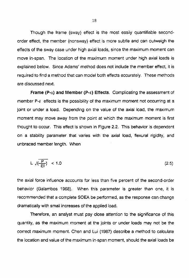
18
Though the frame (sway) effect is the most easily quantifiable second-
order effect, the member (nonsway) effect is more subtle and can outweigh the
effects of the sway case under high axial loads, since the maximum moment can
move in-span. The location of the maximum moment under high axial loads is
explained below. Since Adams’ method does not include the member effect, it is
required to find a method that can model both effects accurately. These methods
are discussed next.
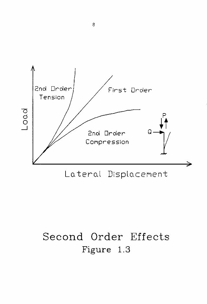
Frame (P-a) and Member (P-5) Effects. Complicating the assessment of
member P-6 effects is the possibility of the maximum moment not occurring at a
joint or under a load. Depending on the value of the axial load, the maximum
moment may move away from the point at which the maximum moment is first
thought to occur. This effect is shown in Figure 2.2. This behavior is dependent
on a Stability parameter that varies with the axial load, flexural rigidity, and
unbraced member length. When
LG) < 1.0 (2.5)
the axial force influence accounts for less than five percent of the second-order
behavior (Galambos 1968). When this parameter is greater than one, it is
recommended that a complete SOEA be performed, as the response can change
dramatically with small increases of the applied load.
Therefore, an analyst must pay close attention to the significance of this
quantity, as the maximum moment at the joints or under loads may not be the
correct maximum moment. Chen and Lui (1987) describe a method to calculate
the location and value of the maximum in-span moment, should the axial loads be

——_ le— Mmax
| — LL Mmax
j | / /
/
P P L <1 < 1 L =T > 1
First Uroder
— — Second Order
Location of Mmax
Figure 2.2

20
of such magnitude to force the maximum along the member length. For the
purposes of this study, the maximum moment is assumed to occur at preselected
joint coordinates, since NUCOR frames generally possess adequate in-plane
flexural rigidity such that the stability parameter described above is less than 1.0.
Convenient methods for assessing the frame and member second-order
effects that involve modifications to first-order analyses were developed by
LeMessurier (1977) and Lui (1988). Both are approximate in application, though
Lui’s method will converge to a correct solution with a sufficient number of
iterations.
LeMessurier’s method is an amplification factor approach that does not
require iteration, but does require lateral translation. It involves calculation of an
individual or story lateral load and a parameter that accounts for the presence of
compressive axial loads. LeMessurier accounts for compressive axial force
influence and also was also intended for prismatic, rectangular framing. It will not
assess the member effect without a lateral translation between the ends of the
member.
A limitation to both the Adams and LeMessurier methods is that
amplification of the design moments is only carried out for columns. The
subassemblage models in these procedures assume the interconnecting beams
act as rigid bodies, and therefore do not participate in the moment redistribution.
The amplification of column moments is not carried over to the connecting beams
or lateral force resisting elements of the bracing system. For these cases, Lui’s
method may be advantageous.
Lui’s method, which has no limiting assumptions (besides the normal
Bernoulli-Euler beam theory assumptions), is applicable to both ASD Types 1, 2,
21
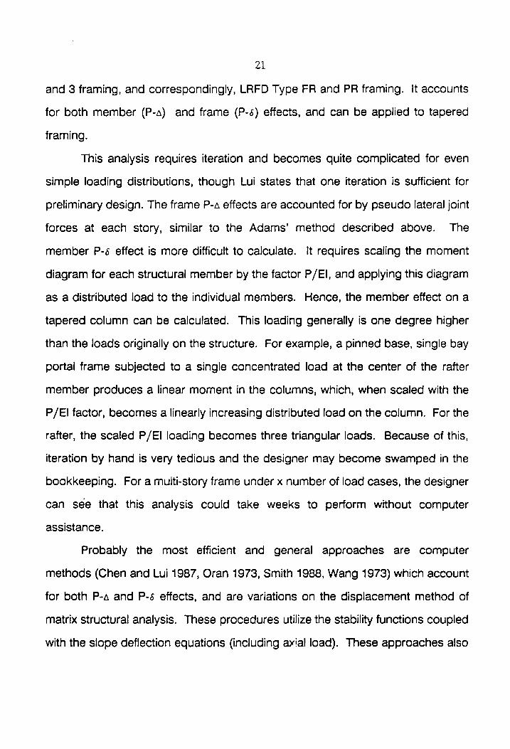
and 3 framing, and correspondingly, LRFD Type FR and PR framing. It accounts
for both member (P-a) and frame (P-6) effects, and can be applied to tapered
framing.
This analysis requires iteration and becomes quite complicated for even
simple loading distributions, though Lui states that one iteration is sufficient for
preliminary design. The frame P-a effects are accounted for by pseudo lateral joint
forces at each story, similar to the Adams’ method described above. The
member P-é effect is more difficult to calculate. It requires scaling the moment
diagram for each structural member by the factor P/El, and applying this diagram
as a distributed load to the individual members. Hence, the member effect on a
tapered column can be calculated. This loading generally is one degree higher
than the loads originally on the structure. For example, a pinned base, single bay
portal frame subjected to a single concentrated load at the center of the rafter
member produces a linear moment in the columns, which, when scaled with the
P/El factor, becomes a linearly increasing distributed load on the column. For the
rafter, the scaled P/EI loading becomes three triangular loads. Because of this,
iteration by hand is very tedious and the designer may become swamped in the
bookkeeping. For a multi-story frame under x number of load cases, the designer
can see that this analysis could take weeks to perform without computer
assistance.
Probably the most efficient and general approaches are computer
methods (Chen and Lui 1987, Oran 1973, Smith 1988, Wang 1973) which account
for both P-a and P-é effects, and are variations on the displacement method of
matrix structural analysis. These procedures utilize the stability functions coupled
with the slope deflection equations (including axial load). These approaches also
22
recognize the increase in member stiffness under the influence of tensile loads
and the decrease in member stiffness under the action of compressive loads.
These methods also require iteration for the nonlinear response, since the stability
functions are dependent on the magnitude and type of axial loads in the
members. However, they are programmable for a computer and iteration
becomes a trivial matter in the overall analysis and design.
Since a matrix-structural analysis approach yields the most efficient and
generally applicable method of analysis, it was chosen as the preferred analysis
tool. The specifics of the solution of equations and system model development
are described in Chapter lll. NUCOR currently uses a first-order elastic matrix-
displacement approach with uniform elements for the analysis of their tapered
frames. With some modifications, it could include second-order elastic analysis
results.
The method of second-order elastic analysis for this study is a two-fold
computer model approach. The structural system model is developed using
element tangent stiffness matrices developed by Oran (1973), and the internal
force-deformation response is developed using element secant stiffness matrices.
In this incremental/iterative approach, response is traced using the system
tangent stiffness as a predictor and the element secant stiffness is used as a
corrector. Figure 2.3 is a graphical description of this approach. As shown in the
figure, the tangent stiffness represents a tangent to the response curve, for the
values of the current displacements. The secant stiffness is calculated from the
initially undeformed configuration (Total-Lagrangian method) and accurately
represents the internal force-deformation response. Applying this method, the
response of the structure up to the elastic stability limit state can be traced.

23 Load
\ \ \ \ \
—--—-— Tangent Stiffness —-— Secant Stiffness
Equilibrium Path
O Current Point
-— a
_| ~~ a
e——— A —~ Displacement
Tangent/Secant Stiffness Figure 2.3

24
Further, since this method uses an exact solution to the beam-column differential
equation, the results are consistent for prismatic geometries (in accordance with
small strains and neglecting shear deformations), but approximate for the finite
element model necessary for tapered beam-columns.
Since the path is nonlinear, the structure must be loaded incrementally,
and iterations performed to converge to an equilibrium point on the response
curve. It is not recommended to apply more than one load increment for a
preliminary analysis/design, as the second-order effects may be overestimated
with the initial structural model elements (White 1990). As the design stage
progresses, the number of load increments can be increased to choose the most
efficient structural sections.
A design criterion has been suggested (Adams 1976, LeMessurier 1977,
Smith 1988) such that the in-plane effective-length factor can be taken as 1.0
when the results of second-order elastic analysis have been used in the member
selection process. Assuming that the in-plane slenderness controls stability,
additional requirements for attempting to utilize K, = 1.0 have also been
suggested:
- Under ASD, the upper limit on the ratio of fa/Fa, calculated at a first-order
effective-length, can be conservatively taken as 0.85 (White 1990). Intuitively
then, for an LRFD approach, the Pu/¢Pn ratio should be limited to approximately
0.9. Except for the lower half of the tapered columns of the frames studied, this
criterion seems to be met.
- The interaction strength as a beam-column may be computed based on an
effective-length factor of 1.0, if the ratio P,,/Py is less than 0.5 (Yura 1987). This
also seems to be met generally for typical NUCOR frames.

25
- Shear deformation is negligible for the buckling mode. Shear deformation
has the effect of lowering the buckling load, and increasing the effective-length of
the column (Galambos 1976). It is only of concern for deep beams.
2.3 Beam-Column Examples
Presented here are two beam-column examples. The first, a member
effect example, and second, a sway effect example. It is shown that the methods
described above may produce different results, supporting the writer’s choice of
using the computer solution method. The same analysis assumptions listed in the
introduction apply to these examples.
Member Effect Example. Given the beam-column shown in Figure 2.4,
which is subjected to a lateral load, Q, at midheight of the column, and
compressive axial force, P, at the top of the column. The member is rotationally
unrestrained at its ends, and not subject to lateral translation (nonsway). The
member is typical of the proportions of H-sections found in the AISC Manuals,
approximately a W14x90 section. It is desired to find the maximum second-order
elastic moments by the theories discussed above.
By inspection, the maximum moment occurs under the lateral load, Q. The
solution of this problem is given by Timoshenko and Gere (1961). The linear
analysis shows no amplification of the design moment, consistent with its theory.
However, when the applicable amplification factor (ASD stability interaction
equation factor on the moment term) is calculated, the degree of second-order
effects has been overestimated according to a correct solution. Notice that with
no sway involved, both the Adams’ and LeMessurier’s methods do not recognize
the increase in moment at center-span (LeMessurier’s model must have chord

26
P Parameters
Q/2 P = 100 kips l \ Q = <0 kips
L QF 6 E = 29000 ksi | I = £987 int
Q/2 L = 200 in
P
Analysis Method M¢ Lin-k1
Timoshenko & Gere 1011.81
Linear 1000.00
Adams P-—Delta 1000.00 LeMessurier P—Delta 1000.00
ASD Amplification 1027.88 Lui’s P—Delta 1011.64
Proposed PDELTA 1011.81 Beam-—Column Problem
(Non—Sway)
Figure 2.4
2/7
rotation). Lui’s method with one iteration (as he suggests) presents a lower
bound, and yields a correct solution. The solution afforded by the proposed
computer method developed as part of this research yields a corrects solution,
since the given problem satisfies the assumptions of the system model.
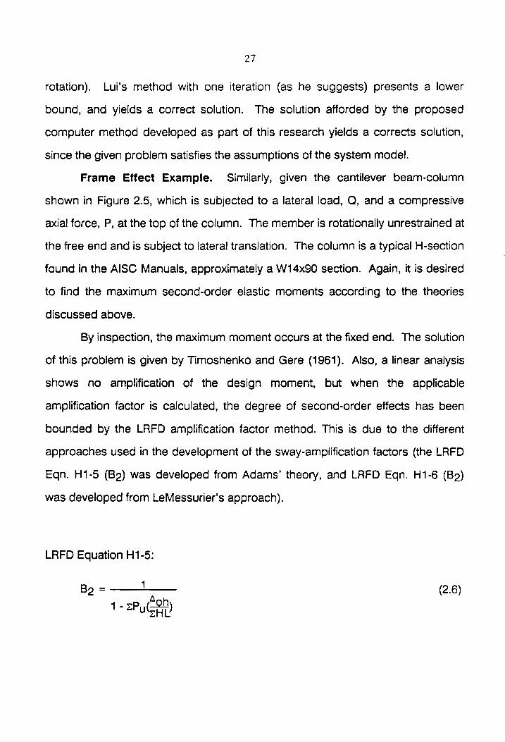
Frame Effect Example. Similarly, given the cantilever beam-column
shown in Figure 2.5, which is subjected to a lateral load, Q, and a compressive
axial force, P, at the top of the column. The member is rotationally unrestrained at
the free end and is subject to lateral translation. The column is a typical H-section
found in the AISC Manuals, approximately a W14x90 section. Again, it is desired
to find the maximum second-order elastic moments according to the theories
discussed above.
By inspection, the maximum moment occurs at the fixed end. The solution
of this problem is given by Timoshenko and Gere (1961). Also, a linear analysis
shows no amplification of the design moment, but when the applicable
amplification factor is calculated, the degree of second-order effects has been
bounded by the LRFD amplification factor method. This is due to the different
approaches used in the development of the sway-amplification factors (the LRFD
Eqn. H1-5 (Bo) was developed from Adams’ theory, and LRFD Eqn. H1-6 (Bo)
was developed from LeMessurier’s approach).
LRFD Equation H1-5:
Bo = —_— (2.6) 1- sPucoh)

28
P Parameters
/
Q—~ 4 P = 100 kips 7 Q = 20 kips
L E = 29000 ksi
| I = 995 int <Q L = 200 in
4M P
Analysis Method M Lin-k]
Timoshenko & Gere 4195.69
Linear 4000.00
Adams P-—Delta 4193.79
LeMessurier P-—Delta 4195.84
LRFD (Hi-5 4238.11
LRFD (H1i-6 4193.78
Lui’s P—Delta 4193.40
Proposed PDELTA 4195.66 Beam-—Column Problem
(Sway)
Figure <.9

29
LRFD Equation H1-6:
1 (2.7)
Lui’s solution with one iteration is close to a correct solution again, as a
lower bound. The proposed computer method developed as part of this research
yields a correct solution, since the given problem satisfies the assumptions of the
system model.
As shown in the beam-column examples, the proposed computer method
gives a correct solution, and is the most convenient and efficient method available
to solve large degree-of-freedom problems. For this reason, the proposed
computer method is employed for this research.

CHAPTER lil
RIGID FRAME MODELING
3.1 Design Loads
The basic design loads were established in order to represent the most
frequently occurring structural loadings. They represent, under a given set of
conditions dependent on geography, the expected loading conditions to which
the buildings will be subjected. To a large extent, NUCOR’s prefabricated
buildings are marketed and designed for the midwestern U.S. region. Typical
structural loads for this region can be found in ANSI A58.1, “Minimum Design
Loads for Buildings and Other Structures,” and the Uniform Building Code (ICBO
1988).
Ground snow loads for this area are typically on the order of 30 psf to 40
psf. The basic wind speed used for the design wind pressures is 80 mph. The
distribution of snow and/or wind loads on the structural frame have been
determined through statistical analysis. The distributions used for this study were
taken from the UBC and the LRBSM. For the balanced and unbalanced snow
load cases, Figure 3.1 graphically depicts the distribution of the snow load.
Tributary areas for each purlin location are computed, and the vertical projection
of the snow load is calculated as a concentrated load, and applied to the rafter.
The wind load distributions shown in Figure 3.2 are taken from the LRBSM, since
the UBC wind load exposure coefficients are currently in a process of amendment
(ICBO 1990). Similarly, the tributary areas of the purlins and girts are calculated,
30

31
a. Full Snow Load
Cq = 1.0 Cq= 0.5
b. Unbalanced Snow Load
Key: -—- Optional Column
Pr 0.7Ca Pg
Snow Load Distributions 1988 Uniform Building Code
Figure 3.1

32
Wind Direction —~—
—1.0 —0.65
0.20- 0.59
a. Wind Case #1
0.65 0.15
b. Wind Case #2
Note: q = 0.00256V* (35 a)!" [psf] H = Eave Height [ft] V = Wind Speed |[mph|
Wind Load Distributions 1986 MBMA Design Code
Figure 3.2

33
and the horizontal and vertical components of the forces are calculated and
applied to the frame components. The distribution coefficients for both snow and
wind have been established statistically.
According to the UBC and the LRBSM, critical load cases are to be
investigated, which cause maximum load effects. Under usual circumstances, the
critical load combinations for single-span, solid-webbed, gabled frames are those
of dead and snow acting together, and dead with snow and wind acting together.
The probability factors of the maximum values of loads occurring simultaneously
is better defined by the LRFD approach, but the ASD load combination factors
have been in use for decades, and are still acceptable.
Acting in combination, i.e., tabulating the loads according to the
statistically-factored load combinations (ANSI A58.1 1982), the effects of snow
and wind occurring simultaneously are developed in accordance with the UBC
provisions. The combinations shown in Table 3.1 are used in this research. The
16 LRFD combinations are shown in order to contrast them with their equivalent
ASD combinations. Notice that the magnitude of the probability factors on the
load combinations are widely different between the ASD and LRFD combinations,
but analytically, are very similar (i.e., maximum snow and half wind, maximum
wind and half snow, etc.). Each of the 16 load combinations needs to be checked
in order to safely establish where and under what combination the maximum
effects occur. The load combination most frequently governing is dead+live
though in some locations other combinations govern. In general, it is necessary
to apply all the combinations to locate the maximum interaction values. This is
true especially for tapered framing, as a frame optimized for one combination may
be unconservative under another. The 16 combinations require the frame to

34
Load Combinations
Allowable Stress Design
oe =———~
ayo
Ne vat
SSaSBER
EE EEE 7+
+ ++
ce t++++
O) w4
~
=
+tunann
SA SUPER eeaas 33
Be ++++4+
+ 00 tt tt
Toe
ttt
Wh
rrr,
Avis +uuaCRSRBae
we mee ae
Hb++hhaag
7+ tt tt
ttagtetet
CLESes
dace d dda
E Hho $++t+te+
tet+tet+ts
anraraaaaat
eT AAAAA
*e
ee eee
eee eee
ne
t uf) WL
a WW
uf)
Load & Resistance Factor Design
aes
BREE steceeenn
AG¢ennococortttttt
+aqeqn
Renee
Stet
stdtdet
att
-
+++
t+teteaaea rt
TT ++
AARAAA
ARARAAAAANAAA AAA
Key:
» n 3 ©
NJ
4990
ie §° 6
we |
i348 Ae iz
ede Pet
ey
ging
= ‘aw .
Sa8 oe
gant
es
0 Ogu
pe Ad gare s WAN
Go
agdee
Table 3.1

35
withstand a variety of structural loadings, from maximum snow to maximum wind
and all variations in-between. The critical load combination generally not known a
priori.
Since the loads to be applied to the main structural framing are given in
terms of a pressure distribution, a discretization is employed to model the load
transfer. Since the given loads are transferred to the primary frames through
simple-span purlins, the loads induced on the frames are of a concentrated type.
The concentrated loads are determined by calculating the tributary area of each
purlin, and multiplying this square-foot area by the values of the tabulated
pounds-per-square-foot basic load. These equivalent concentrated loads are
then applied to the structural model, just as they would be applied to the actual
frame. The calculations must also account for slope of the roof, in order to
determine vertical and horizontal concentrated loads at each purlin or girt. These
calculations are trivial and not repeated here, but are developed by the standard
vector transformations.
Note: The analysis program written for the study does not account for
uniform loads, since the frames studied are subjected only to concentrated loads,
provided at purlin or girt locations. Element selfweight is actually a distributed
load, but was discretized into equivalent concentrated vertical forces at the ends
of the elements. The fixed-end-moments due to the uniformly distributed
selfweight, consistent with the FEM, was neglected. This is done due to the fact
that the dead load of the structure is negligible for these types of frames, and
would only further increase the analysis time by accounting for these trivially small
moments.

36
3.2 Frame Discretization
The structural model is developed through a segmental discretization,
called elements. These elements join points that are of particular interest to the
analyst. The joints are selected in order to describe the behavior of the structure
in an overail way, as the element model does not give the continuum behavior. Of
particular interest in unbraced rigid frames, are the lateral movements of the tops
of the columns (drift), the vertical movement at the gable, the rotations at the
bases of the columns, etc. With the knowledge of behavior at specific points of
interest, the frame can be designed to withstand the structural loadings.
A prismatic, single-bay portal frame can be represented with only three
elements, one each for the columns, and one interconnecting beam, according to
the first-order elastic matrix displacement method (MDM) of structural analysis.
However, the use of these prismatic elements to model the behavior of a tapered
beam can introduce severe discretization errors (Yang 1986). This discretization
must be chosen carefully in order to minimize the potential error. The use of
uniform elements in the model of a tapered beam goes beyond the theory of the
matrix displacement method. Its roots are in the finite element method (FEM),
and should be treated as such. Note that the FEM degenerates to the MDM, for
the case of prismatic members.
In the first-order elastic analysis of prismatic structures then, not much
thought is required in developing a suitable model, once the analyst is familiar with
the process. However, for a second-order elastic prismatic beam-column
problem, selection of the proper number of elements for an accurate model is
another subject. White (1990) suggests a crite-ion for element selection, based
on the value of the expected maximum axial load and its Euler buckling load. This

37
criterion is that the quantity P/Pe is held to be below 0.4. It is suggested that a
typical beam-column of prismatic section requires a maximum number of three
elements to hold the error to less than 1%. (White 90) Since this study is to model
tapered beam-columns, the writer recommends that this upper bound be used as
a lower bound for the element selection, as discretization errors are introduced by
selecting too few elements. Appendix C discusses the reason for this suggestion.
The error introduced by the use of uniform elements can be quite
substantial, and is the subject of Appendix C. Minimization of this error can be
accomplished by using a higher number of prismatic elements, or using an
element model that was developed as possessing a taper. The use of tapered
elements can reduce the number of degrees of freedom in the analysis, thereby
reducing analysis time. The discretization of the frame into the elements
described above is the subject of the next section.
3.3 Element Models
Section 3.2 describes the discretization of a structural model through the
analysts’ identification of points of interest. These points of interest are labeled as
joints or nodes. Whether or not two or more members actually intersect at the so-
called joint is not important. A joint can be placed anywhere. In a two-
dimensional plane frame, each joint possesses three degrees of freedom (DOF)
i.e., the horizontal and lateral translational components, and a rotation.
Quantifying the amount of deformation at each of these DOFs, the behavior under
a particular load combination can be shown by drawing the displaced state of the
structure. Between each of these joints, a beam-column element must be defined

38
to store the induced flexural and axial energies introduced by the loading. These
elements are defined next.
After global degrees of freedom are selected, the elements between them
are identified and transformed into the global set of stiffness equations. Figures
3.3 and 3.4 show a typical prismatic beam-column element labeled with its
elemental degrees of freedom for both the global and member system. Once
these elements are mapped into the system of stiffness equations, and the
system is solved for the displacements at the joints, the element forces can be
determined. Figures 3.5 and 3.6 show the beam-column element labeled with its
elemental global and local force systems, which are calculated first by the joint
forces, and then rotating them with the standard transformation matrix.
It is important to remember that this research does not follow the usual
procedure of the MDM, not only because of the tapered frame behavior, but also,
and primarily, because of the required nonlinear analysis. As described above, a
tangent-stiffness was used to predict response and a secant-stiffness was used to
model the internal force-deformation behavior. Because of these differences, the
element model used to map element stiffnesses into the system model is different
from the element model used to determine the internal response.
The element tangent stiffness matrices used in this research were
developed by Oran (1973). Figure 3.7 snows an element global tangent-stiffness
matrix, in notation identical to that of Holzer (1985), except for the ¢ terms on the
rotational stiffness terms. These ¢ terms reduce(increase) the amount of stiffness
present at these terms under axially compressive(tensile) loads. If the axial load is
neglected or zero, the stiffness matrix will reduce to the standard first-order beam-
column element matrix.

39
Element GDUF Definition
Figure 3.3
S by
©
VS
‘5 S Element LDUF Definition
Figure 3.4

40
FD
F6 ord
Fe ©
F 3 F
A) Element Global Forces
Figure 3.0
NES Ps
w\3
Ne
We © Element Local Forces
Figure 3.6

41
| €,| &. |-B2 -8,/ &;
| g 6 -g 4 -£ 5 S — | . EI
K, = as L
g= AL 8, | 82 |-84 I
c, = coso _
Cc = sinQ 8 3 8 3
Symmetric g.
2, = X(Be? + 2c¥dy) Compression
g. = XC,Co( B- 2s) 6, = kL(sin(kL)—kLcos(kL))/$,
B= 2(Bc$+2c%o,) 2 = KL(kL-sin(kL))/¢ By =—AdgLC,
g, = aAdgLec, Tension
£.= ad, L? , = kL(kLcosh(kL)—sinh(kL))/$,
g., = Xoz1" bo = kL(sinh(kL)-kL)/o,
Where: 6. = 2~—2cos(kL)—kLsin(kL)
6, = 2-2cosh(kL)+kLsinh(kL)
Tangent Stiffness Matrix Figure 3.7

42
As an abstraction, it is interesting to note that the geometric stiffness matrix
for a beam-column that is usually used to represent the tangent stiffness was
compared with that of Oran’s. It was found that Oran’s tangent stiffness
converged to the solution faster than that of the usual matrix. For this reason,
Oran’s matrix was used rather than staying with usual practice.
The element secant stiffness matrices (shown in Figure 3.8) used in this
research are taken from Chen and Lui (1987), and represent the internal force-
deformation behavior of the element, consistent with the exact solution to the
differential equation. The element model was developed for end moments,
shears, and forces, with no in-span lateral loads. Again, should the effect of axial
load on the flexural stiffnmesses be neglected, the stiffness matrix will reduce to the
standard first-order beam-column element matrix.
3.4 System Model
The system model is assembled according to the usual mapping of
element stiffness terms into the global stiffness matrix. The computer program
stores the stiffness terms in a single column vector, and the locations of elements
of the main diagonal are stored in a column vector. This technique is employed in
order to optimize the solution process, taking advantage of symmetry of the
system stiffness matrix. Because of symmetry, and the fact that the system
Stiffness matrix is closely banded to the main diagonal, a solution technique called
the active column solver is utilized. This facilitates faster solution, since storing
the entire DOFxDOF system stiffness matrix would unnecessarily require the
storage of large quantities of zeroes, and mathematical operations on them. By

A _A r 0 O -F 0 O le, 6 —le, 6 me ph 0 Fate,
—6
k_= = #93 . Lees
7 0 0 T le, —6
K. =N\k g /\ 2 o, L eo,
Symmetric 4%,
Compression Tension
in (kL)> sin(kL) (kL)> sinh(kL) 1 12%¢ 12 9,
(KL)? (1-cos(kL)) (kL)* (cosh(kL)—1) 2 6D. BP
b (k1)(sin(kL)—kL(cos(kKL)) |(KL)(kLcosh(kL)—sinh(kL))
3 4Pc 49, d (kL)(kL—sin(kL)) (kL)(sinh(kL)—kL)
4 2 P- eC D+
Where: 0. = 2-2cos(kL)—klsin(kL)
O, = 2—2cosh(kL)+kLsinh(kL)
Secant Stiffness Matrix Figure 3.8

4d
this method, computer memory requirements are reduced, and the solution
progresses at a faster pace.
Probably the largest disadvantage to a nonlinear problem is the solution
effort required to solve the systems of equations. With the element stiffness
matrix coefficients dependent on the magnitude and direction of the axial load, the
loss of superposition is of a serious nature. With a second-order elastic analysis
of the type used here, the system of equations must be solved for each load
combination, load increment, and equilibrium iteration. This means that for
sixteen load combinations, three load increments/combination, and (say) five
iterations per increment is required for equilibrium, the entire system of equations
is solved 32*3*5 = 480 times. Obviously, this is best suited to computer solution.
The analysis scheme is discussed next.
3.5 Solution of System Equations
Figure 3.9 shows the differences between the requirements of a first-order
elastic analysis and a nonlinear, second-order elastic analysis technique. The
flowchart is shown in the format presented by Holzer (1985), with the
modifications required for the nonlinear analysis shown. This is done to begin to
describe the effort involved in performing a nonlinear analysis. As indicated, an
FOEA follows the dashed lines on the chart.
The response is solved by Newton-Raphson iteration. Since the
displacements are unknown initially, so are the axial forces. When the first
increment of load is applied to the system, a first-order elastic analysis is
performed. With this information, the axial loads for this level of displacement and
applied load can be determined. Then, the axial loads are used to check the

45
1. Unknowns
q
2. Element 6. Element 7. Joint
Models Forces Forces
—f=kd+f-—- — f }——~P =rF
3. System 5. Element Model Models
Kiq = Q f=kd+f
—— — First Order 4. Solution Analysis
—-4 4
8. Residual Check
No
(Q—P)=0?;}——+ Go to 2.
Yes
Stop
Note: Process identical to conventional first order analysis, with modifications to trace the nonlinear equilibrium path.
Matrix Displacement Method for Second Order Analysis
Figure 3.9

46
equilibrium of the structure, and a residual load vector, if necessary, is applied to
the structure. Essentially, the nonlinear response is solved by employing a series
of linear analyses. This procedure is sometimes called quasilinearization. The
process for locating a single equilibrium point is shown in Figure 3.10. A single
equilibrium point using the Newton-Raphson solution technique usually requires
three or four iterations to locate. Because of the nonlinear response, both
accrued load level and accrued displacements must be maintained.
Convergence of the process requires two criteria to be satisfied for this Newton-
Raphson scheme.
In order to determine if an equilibrium point has been located, two separate
criteria must be checked. In a general first-order elastic analysis utilizing the FEM,
displacement analysis is a convergence problem. Here, because of the nonlinear
equilibrium path, both displacements and the internal forces must converge. This
can be demonstrated by two diagrams.
The displacement convergence criteria is required to determine whether or
not the structure has deformed an appreciable amount, i.e., enough to warrant
applying another iteration. Bathe (1976) and Cook (1989) both recommend a
relative displacement target value of 1/1000 be a cutoff point for convergence.
This behavior may be visualized by the response of a beam-column under
compression and transverse loading. This is a stress-softening phenomenon, as
shown in Figure 3.11. It shows that even though the internal/external forces are
within a tolerable difference, the increment in displacement is not within
tolerances.
Similarly, force convergence criteria is required to determine whether or
not the load imbalance between that stored internally and that applied externally is

Load
47
Key: Ks Secant Stiffness
Kt Tangent Stiffness Q Current Load Level R Current Residual
Equilibrium Points: i — “Initial” Configuration j — Current Configuration k — Sought Configuration
Ay 42 _ _L | ss
Deformation
Newton Raphson Iteration to Load Level °Q.” Tangent and Secant Stiffnesses are formulated at the last equilibrium point found. Convergence is attained when both the increment in deformation and the value of the residual are within their respective tolerances.
Full Newton-Raphson I[teration
Figure 3.10

48
ITE end
ped1aaAuoy
JON ‘duUTUSJOS
Ssazy¢
yUuaWUIINeTdSIG
/N
vl vl
peo]

49
enough to warrant another iteration. Bathe (1976) recommends a relative force
target value of 0.1 be the cutoff point for convergence. This behavior may be
visualized by the response of a beam-column under tension and transverse
loading. This is a stress-stiffening phenomenon, as shown in Figure 3.12. This
shows that even though the increment in displacement is within a tolerable
difference, the imbalance in the load is not within tolerance.
By the above discussion then, it is necessary to satisfy both of these
convergence criteria simultaneously. The computer program developed as a part
of this study uses these criteria, with a slight change in application. Rather than
tracing and forcing convergence at each degree of freedom, those locations
accruing the largest incremental deformations or largest load imbalances were
compared with the convergence criteria. Because of the interdependence of the
displacements and forces, the technique utilized here will bring about sufficient
accuracy, such that when an equilibrium point is assumed, the residual vector is
essentially zero, and the displacement increments are likewise, zero.
Normally, the number of load increments applied to each of the structures
is also a variable, because with fewer updates of the system matrix, the solution
may drift from the theoretical solution, and result in the system stiffness being
overestimated. This situation is avoided by the tangent/secant stiffness model
employed here, because the secant stiffness matrix presented correctly models
the internal force-deformation response.
The final variable of these analyses is that of the iterations to be performed.
Again, since the loads are of practical concern, the maximum number of iterations
to find a single equilibrium point was set at 20. White (1990), states that a
practical limit of 10 can be imposed.

50
ote andy
podJOAUO)
JON ‘sUIUATIIYS
ssouys
yuaUIa0B[dsSIG
N
ey || Wy
peo'T

CHAPTER IV
SECOND ORDER ELASTIC ANALYSIS AND DESIGN
4.1 Introduction
This section of the study focuses on the development of the design
equations of the ASD and LRFD Specifications. Although the ASD Specification
was not developed formally to be used with second-order elastic analysis, the
analyst can judge by analogy the rules to follow. The LRFD Specification always
requires second-order elastic analysis of beam-column members. Because of the
difficulties of implementing Specification requirements for slender cross-sections,
example capacity determinations are provided in Appendix D.
4.2 Allowable Stress Design, First-Order Approach
The use of first-order elastic analysis with the allowable stress design
procedure is common practice. The philosophy of ASD is to design elements to
resist imposed loads by a margin of safety. This margin, known as a factor-of-
safety (FS), varies with the type of applied stress (flexural, axial, shear). For
example, the FS for shear on rolled beams is 1.44. This can be back-calculated
by using the von-Mises octahedral shear yielding criterion, which defines shear
strength to be Fy//3. AISC specifies the allowable stress to be 0.4Fy. Calculating
the ratio of (Fy//3)/0.4Fy obtains the value 1.44. In general, the format can be
described by:
51

52
—1 > 5m (4.1)
The notation of Equation 4.1 is: Rn/FS = nominal capacity / factor-of-safety, and
= Qm = sum of the service load effects. Or, essentially that the section strength,
divided by a margin of safety, must be greater than the effects caused by the
expected loads. Notice that "safety" is measured in terms of the expected service
load range.
Moving onto specifics, two interaction equations must be satisfied for a
compressive beam-column member. For tensile beam-columns, only one of the
equations need be checked. These equations are known as the stability and yield
interaction equations. Note here that the yielding equation is somewhat of a
misnomer, as the flexural term of this equation can sometimes be based on
lateral-torsional buckling or local-buckling.
The ASD Stability Interaction Equation (1978 or 1989) is
f f | 2 + Sin ees 1.0 (4.2)
a (1-—a)'P F'e
and the ASD Yielding Interaction Equation (1989) is
f, of a Ob. O6QF, * F<!” (4.3)
The stability interaction ratio (compression only) is based on the axial
Capacity and flexural strength of the section as though failure was imminent,
according to Salmon and Johnson (1989). This means that the column strength

93
used in the equation is the absolute design maximum value of stress that the
section can safely resist. This should be emphasized because of a slender
member design problem, discussed later. The effective-length of the column is
chosen by a rational method and is an inconvenient though necessary evil of first-
order elastic design. The flexural strength is developed as though the member
were subjected to purely flexural stresses.
Emphasized again, Fa is the absolute design maximum value of the
compressive strength at effective-length and _ effective-cross-section. For
prismatic, rectangular structures, the effective length factor [K] is usually
determined by the use of Julian and Lawrence’s effective-length factor
nomographs (AISC 1989). For tapered members, Lee (1972) developed the
effective-length nomographs using the Rayleigh-Ritz procedure and infinite series
solution. The development of the nomographs is beyond the scope of this study.
NUCOR assumes that the in-plane effective-length factor for tapered columns is
1.5. They also assume that the in-plane effective-length factor for tapered rafters
is 1.95. Other means are available to estimate this factor, and are considered in
Chapter VI. The factor-of-safety in the stability interaction equation is
approximately 1.67 against elastic instability.
For the yielding interaction ratio, the factor-of-safety in this equation is
approximately 1.67 against yielding of the extreme fibers of the cross-section.
4.3 Allowable Stress Design, Second-Order Approach
The philosophy of these design rules is based partly on criteria suggested
by SOEA researchers Adams (1976), LeMessurier (1977), and Smith (1988). The

54
design interaction equations are identical in format with those of the first-order
design rules, with some modifications of the terms involved.
Practically speaking, the amplification of moments in the stability interaction
equation provides an estimate of the second order effects. Logically then, if frame
and member second-order results were accounted for directly at the analysis
stage, the amplification factor could be eliminated in this equation. The extension
suggested by Adams is that the effective length factor may be taken as 1.0 for the
interaction check. White (1990) suggests that Kx = 1.0 is only applicable when
fa/Fa < 0.85, and Yura (1987) suggests that Kx = 1.0 may be applicable when
Pu/Py < 0.5, as noted previously. Assuming that these criteria are met, the
incrementally-applied second-order ASD stability interaction equation is given by:
f, f 28 + zs 1.0 (4.4)
a b
where fp and Fp are respectively, the calculated second-order moment and
allowable moment at specific locations under investigation. When used in this
format, it intuitively compares with the LRFD interaction equations, shown below
as equations (4.6) and (4.7).
The difference in the yielding interaction equation is that the second-order
elastic moment is used in the interaction check, rather than the first-order elastic
moment. Though the first-order ASD yielding interaction equation uses first-order
elastic moments, it was thought to be inconsistent with the development here, so
the calculated second-order moments are used instead of the first-order
moments.
55
The proposed benefit of an ASD second-order analysis and design
philosophy is in the stability interaction equation. The increase in the flexural term
by SOEA may be larger than the increase predicted by the first-order ASD
amplification factor, and could possibly offset the accompanying decrease in the
axial term. It is noted here that if the out-of-plane slenderness ratio controls the
column strength, there may not be a benefit in using second-order elastic
analysis, since the effective-length factor cannot be modified. If out-of-plane
slenderness controls, the only possibility of benefit is that the actual second-order
moments may be smaller than those obtained by the first-order ASD amplification
factor analysis. Under the current first-order design rules, if the yielding ratio is
governing, the use of SOEA only results in higher moments under axial
compression. Therefore, no benefit is possible. If an SOEA converges, the
structure is not unstable elastically, but may still be unstable inelastically. The
stability interaction equation is really an inelastic stability interaction equation, but
is more commonly called the stability interaction equation.
4.4 Load & Resistance Factor Design Approach
Load & Resistance Factor Design requires the use of second-order elastic
analysis results. Also, the provisions of the LRFD Specification were developed
assuming factored loading. The format of LRFD is to design structural systems to
resist maximum expected lifetime loads, hence the need for factored loads. The
load factors and material reliability factors were determined by probabilistic
analysis. Load factors were probabilistically determined according to measured
maximum values, and the probability of different types of loadings occurring at
their maximum values is considered in the load combinations. Material strength

56
reduction factors are determined based on observed statistical data on specified
versus delivered section properties. This philosophy results in a more uniform
reliability of the structure under different load combinations. The LRFD
Specification attempts to obtain a uniform reliability over the entire structural
system.
In general, the philosophy of the design approach is,
m
Rp == yQm (4.5)
Where ¢ = strength reduction factor, Ry = nominal strength, = = summation over
m, y = load factor, Q = service load effect m. Or, essentially that the nominal
section strength multiplied by a strength reduction factor must be greater than the
effects caused by the sum of the factored loads. Notice that safety here is
measured in terms of a factored load range. One stability-based bilinear
interaction equation must be satisfied for a beam-column member. The portion of
the design curve to be followed is determined according to the axial force ratio.
The 1986 LRFD Specification interaction equations are:
For Py/¢Ppy > 0.2
P M U4, 8 uu aP,, +6 3M, 1.0 (4.6)

57
For Pu/¢Pn < 0.2
p M Tu, Mu Bp * GMS 1.0 (4.7)
The significance of the first term of the interaction ratio is the same as that
of the ASD stability interaction equation. All unity strength checks are performed
with the denominators (strengths) at their nominal capacities. The nominal
Capacities are determined based on a limit-states analysis approach and
represent the strength that can be obtained, as in a laboratory experiment under
controlled conditions. This strength is then reduced by ¢ factors, which are based
on tolerances of the available section strength.
When compared with the alternate interaction equations (braced frames
only) in Appendix H of the 1986 LRFD Specification, Equations 4.7 and 4.8 seem
overly conservative for all values of column slenderness ratios. Though not
specifically stated, it is believed that the Appendix H equations are to be used only
when plastic strength is attainable.
4.5 Comparison of Specification Provisions
The following discussions concern the nominal strengths of cross-
sections, neglecting the /oad effect side of the total design equations.
4.5.1 Flexural Strengths
For the plastic region of flexural strength, LRFD utilizes the correct plastic
moment, not an assumed 10% increase from the moment which causes first-yield
on compact cross-sections. The cross-sections of NUCOR frames are rarely

58
capable of developing a fully-plastic moment, as the compact section criteria are
usually violated. Though LRFD utilizes a higher strength in this region, it is
generally unavailable to typical metal buildings.
For the lateral-torsional buckling strength region, although the strengths in
LRFD directly account for both the warping and St. Venant torsional resistance
terms, ASD permits use of the vector sum of these individual allowable flexural
stresses. A modified ry (r7 is normally the weak-axis radius of gyration of a
portion of the cross-section, comprising the compression flange and 1/3 of the
compression web area) must be calculated for this purpose. Therefore, the
difference between the two specifications has been eliminated in this respect.
The modified ry equation is shown in Chapter VU.
LRFD has separate limit state strengths for flange local buckling (FLB) and
web local buckling (WLB). However, ASD does not have a comparable WLB
provision. This is an ASD benefit, but WLB can still occur even though it is not a
recognized concern of the ASD Specifications.
LRFD was calibrated to produce similar results as a first-order ASD
produces at an L/D ratio of 3.0. However, this calibration seems to apply only
when dead and live load are involved. When wind loadings are included, LRFD
does not recognize a 1/3 strength increase.
The lower curve of Figure 4.1 describes a first-order elastic behavior
required strength comparison between ASD and LRFD for tensile or flexural
members (with noncompact section), varying the L/D ratio. Values on the graph
less than 1.0 indicate economy in favor of LRFD, and values greater than 1.0
indicate economy in favor of ASD. This plot is only for the dead+live load
combination. The lower plot describes a first-order comparison of the results to

LRFD
/ASD
Ratio
39
LOAD COMBINATIONS
LRFD vs. ASD
1.5
1.4
1.3
1.2
1.1
1.0
0.9
0.8
W/D = —1.5 [(1.2+1.6*L/D+0.8*W/D)/0.9]
[(5/3)(1.0+L/D+0.5*W/D)]*0.75
[(1.2+1.6*L/D)/0.9] [((5/3)(1.0+L/D]
0.7
L/D Ratio
Figure 4.1
10
60
be expected when comparing ASD with LRFD. Consider a tension member or a
noncompact flexural member to be the member being designed. As the graph
shows, at aL/D ratio of 5.0, LRFD requires a section with 2.2% higher strength.
However, this situation is only part of the whole story. This 2.2% required
increase is not typical, as the upper plot describes. When other ASD load
combinations are compared, such as dead+snow+wind/2, ASD allows a 1/3
stress increase, whereas LRFD does not, since it is based on a philosophy of
maximum expected lifetime loads. The second plot in Figure 4.1 shows a pure
flexure or pure tension member with dead, live, and wind loads. The wind load is
held constant here (uplift is assumed), and there are no second-order effects
considered. Notice that the curve approaches a value of 1.33, indicating that ASD
is more economical by nearly 33% over an LRFD approach for this range.
However, because of the magnitude of loads and geometry of the typical NUCOR
frame, the controlling ASD combination is usually D+L, and in LRFD it is either
1.2D+1.6L or 1.20+1.6L+0.8W.
For weak-axis flexure of H cross sections, LRFD provides a great deal of
strength compared to that of the ASD. This is due to the assumption of full
plastification about the weak-axis. Unfortunately, weak-axis bending is not utilized
for the primary load-resisting elements of these rigid frame gabled structures.
4.5.2 Axial Compressive Strengths
The equations governing compressive strength of noncompact sections in
ASD and LRFD essentially follow the same capacity curve, although LRFD
assumes a Slightly different residual stress distribution of 0.44Fy instead of
0.50Fy. This has the effect of allowing it a larger inelastic strength zone. However,
when the LRFD closed-form tapered member provisions are followed, the

61
inelastic/elastic cutoff point occurs earlier, (lower column slenderness ratios)
indicating a larger elastic zone. Whenever the elastic zone is used, the strength is
smaller than that achieved through inelastic action.
When slender cross-sections are involved, LRFD also possesses greater
strengths, especially when compared to the 1989 ASD Specification. This
situation arises from the fact that the Q, factors in the new ASD Specification drop
off sharply due to the flange/web local buckling interaction formulas.
4.6 Future Specification Modifications
As seen in Figure 4.1, inconsistencies with LRFD need to be worked out.
There are other problems with the 1986 LRFD Specification, including but not
limited to shear strength. For compact/noncompact sections compared with
ASD, the LRFD shear strength is approximately 10% lower (Wishart 1990), and
the strength equation may be changed in future editions of this Specification. The
strengths are nearly identical for slender-web sections. Other potential problems
involve the tapered member design provisions (though these are not typically
followed by the industry). It is believed that the metal building industry follows the
prismatic beam provisions, developing the section strengths at incremental
locations along tapered members. This procedure is also followed in this
research.
Further, it was recognized that research sponsored by Butler
Manufacturing concerning flange/web local buckling that found its place in the
1989 ASD Specification was not incorporated into the LRFD Specification.
Because of the omission, there exists an envelope of economy in favor of LRFD.
Under pure flexure, and an L/D ratio of 5, there is an approximate 12% increase in

62
flexural strength, depending on flange and web proportions. This can be
visualized by Figure 4.2. The writer believes that either this 1989 ASD
Specification criterion is incorrect, or the 1986 LRFD Specification is incorrect for
this range. This should be studied further for applicability.
The upper graph of Figure 4.2 represents the available allowable stresses
(ASD) and the reduced nominal capacities (LRFD) according to each of the
design equations (labelled on the graph for convenience). FLB, WLB, and PG are
abbreviations for flange local buckling, web local buckling, and plate girder,
respectively. The graphs were constructed for a beam with 7 in. x 0.3125 in.
flanges, 0.2060 in. thickness web, Fy = 50 ksi, and welded plate construction.
The depth of the section was varied in order to trace the response that a tapered
member would provide. Lateral-torsional buckling is assumed to be prevented.
According to the 1978 ASD Specification and the 1986 LRFD Specification,
the section is partially compact up to h/t = 138. By the 1989 ASD Specification
however, the flanges are partially compact up to an h/t value of 70. Past this
point, the flange slenderness local buckling limit is dependent on the web h/t
ratio. With this difference, the allowable stress then follows a transition curve from
0.63Fy to an intersection point somewhere on the plate girder design curve. The
0.63Fy is obtained from the provisions of F2 (1989 ASD), since the section
possesses a noncompact flange and compact web in this region of h/t.
An economic envelope was found to exist in the region between this new
ASD curve and the LRFD curves. As an example, assume the following:
- Live + Dead load combination controls.
- L/D = 5.
- h/t = 120.

Flex
ural
St
ress
[ksi]
Flex
ural
St
ress
[k
si]
60
50
40
30
20
10
60
30
40
30
20
10
63
Available Flexural Stress
WLB FLB
LRFD PG
FLB
\ N
TT
ASD F/W LB pe
S __I j t 1 J
40 80 120 160 200 240
Web hc/tw Ratio
LRFD Envelope 1986 Specification
ASD Envelope
- 1978 Specification
1989 Specification - oN
[70 [38
| 7 a ] : t I I
40 80 120 160 200 240
Web hc/tw Ratio
Figure 4.2

64
Design stresses from the plots are:
1978 ASD: Fh = 32ksi
1989 ASD: Fp = 27 ksi
1986 LRFD: ¢F, = 47 ksi
Comparing the design stresses (unfactoring the LRFD effect):
1986 LRFD versus 1978 ASD:
[47 ksi] /[32 ksi] /[(1.2 + 1.6(5))/(1+5)] = 0.96;
therefore ASD is economical by 4%
1986 LRFD versus 1989 ASD:
[47 ksi] /(27 ksi] /[(1.2+ 1.6(5))/(1+5)] = 1.14;
therefore LRFD is economical by 14%
This difference of 14% is applicable only under pure flexural loading. When
second-order beam-column effects are included, the economic envelope gets
smaller, but is still greater than approximately 3%.
This omission will be under study by the LRFD Specification Committee for
possible inclusion in the 279 or 3°9 Edition. However, it is not on the current
agenda for the 2nd | RFD Specification, indicating that this envelope will be
available for at least four more years. Also, the AISC had taken the position that
the flange/web local web buckling interaction would not have much affect on the
metal building industry. The writer feels that differences of approximately 10% are
a serious consequence, and that the range of applicability of the ASD equation be

65
researched further. With this current criteria, a significant portion of flexural
strengths for slender- flanged cross-sections will fall into this category.

CHAPTER V
CASE STUDIES
5.1 Introduction
This chapter focuses on the results of applying the SOEA rules to the frame
geometries submitted by the sponsor. There are three alternative design
calculations for each frame, not including first-order ASD results.
Each of the 10 frames is analyzed for 16 ASD load combinations, and the
corresponding 16 LRFD load combinations. The results of the analyses are then
input to specification checking programs and the maximum interaction ratios are
tabulated. The relative economy of each of the three alternatives is then
compared by calculating the average percent difference between the first-order
ASD ratios and each of the three alternatives.
5.2 Method of Comparison
For all the frames studied, the results are compared to the first-order
analysis results. For each element of each frame, the maximum interaction ratio
from its governing limit conditions is calculated. These limits may occur over one
or more load combinations, i.e., stability under load combination 1, yielding under
load combination 6, shear under load combination 8, etc. Generally, for
symmetric gable frames, the first-order interaction ratios are controlled by the
D+S and D+S+W/2 load combinations. Under LRFD, the governing load
66

67
combinations are 1.2D+1.6S and 1.2D+1.6S+0.8W. Summary graphs of each
frame and the design proposal interactions are found in Appendix A.
The economic comparisons are obtained by dividing the individual element
interaction ratios by their first-order interaction ratios. By this method, multiples of
the controlling first-order interaction ratios are found.
As an example, assume that a theoretical comparison is being performed
between ASD and LRFD. Further assume that the LRFD strength interaction ratio
is calculated to be 0.90. Likewise, assume that a first-order ASD is performed on
the same member, and the governing interaction ratio is calculated to be 0.95.
Normalizing the results,
LRFD/ASD = 0.90/0.95 = 0.9474
gives the multiple of the first-order interaction for LRFD vs. ASD. For this example
then, LRFD is more economical than ASD by an amount:
(1.0-0.9474)*100% = 5.26%
When comparing ASD with LRFD, there can be confusion between
strength comparisons and load effects comparisons because of the load and
strength factoring. Comparing normalized interaction ratios eliminates any
confusion.
Economy is provided by those multiples that are less than 1.0. These
multiples are then analytically assessed as to their relative economies on a
percentage basis. This was accomplished by defining a spreadsheet for each

68
frame, listing the maximum interaction values for each of the analysis types. With
this information, the multiples of the first-order ASD ratios are easily found.
Graphs were then created in order to facilitate a quick data presentation.
Specification checking computer programs written to accept the results of the
analysis program were implemented here. The maximum interaction ratio of the
selected cross-sections of each frame was extracted by these programs. The
spreadsheets were also used to develop the average increase or decrease in the
responses.
5.3 Economic Criterion
Economy, as used in this study, is defined as an available increase in
design strength of at least 3%. It was assumed that an increase in design
strength smaller than 3% would not justify the increase in analysis time required
by second-order analysis.
5.4 Preliminary Data Cautions
Originally, the frames were designed under the 1978 ASD Specification.
Due to the availability of the 1989 ASD Specification and its amendments to
slender cross-section design, this research attempted to investigate frame
integrity according to this new ASD Specification. The writer believes that there
may be some confusion in application of slender cross-section design rules. To
assist in alleviating this confusion, the provisions for slender cross-sections are
discussed in Appendix D.

69
At various locations along the frames, the first-order design interaction
ratios are considerably greater than 1.0. This is primarily due to four causes.
They are:
- The flange/web local buckling interaction formula of the 1989 ASD
Specification was included for flexural strengths;
- Compression allowable stresses were calculated for the condition of
imminent failure (Salmon and Johnson 1989), iterating with f=Fa when slender-
web cross-sections are involved;
- Inclusion of the form-factor Q in denominator of the axial term of the 1989
ASD yielding interaction formula;
- Investigation of unbalanced snow load distributions, which were not
Originally investigated.
With the intent of satisfying the research proposal requirements of
assessing P-Delta effects and critiquing LRFD of Gable Frames, three alternate
design procedures (proposals) are defined as follows:
- The first alternate is a second-order elastic analysis and design check
according to the Allowable Stress Design rules developed in Chapter 4, Section 3.
This is identified in the individual discussions by the notation ASD\so.
- The second alternate is a second-order elastic analysis and design check
according to the Load and Resistance Factor Design rules developed in Chapter
4, Section 4. This is identified in the individual discussions by the notation LRFD.
- The third alternate is a first-order elastic analysis and design check
according to the Allowable Stress Design rules developed in Chapter 4, Section 2,

70
but does not use the effective-length factors that NUCOR usually assumes.
According to elastic stability analyses and the tapered-column effective-length
factor charts found in the Commentary to the ASD Specification (AISC 1978, AISC
1989), reduced (in-plane) effective-length factors were found to be available.
They were Kx = 1.3 (columns) and Ky = 1.85 (rafters). Their development is the
subject of Chapter VI. This is identified in the individual discussions as ASD\p.
Also, ASD\fo denotes the ASD first-order design, according to the
assumed NUCOR K, values.
In Appendix A, these results of each of the alternate design checks are
plotted over their location on each of the frames. All interaction ratio multiples are
measured with respect to the ASD\fo behavior.
5.5 Frame Discussions
The designation of each of the frames has the following format:
aWIDE bEAVE ¢/12 dPSF
Where a = total width of building frame (ft.), b = vertical height of the eave (ft.), c
= roof slope from the eave to the gable point, as a function of 12 in., and d = the
value of the snow load (psf.) applied to the horizontal projection of the frame.
The horizontal axes of the graphs in Appendix A represent cross-section
locations along the frame. These locations start at the base of the left column and
traverse the frame to the right column.

71
5.5.1 Frame #1; Designation: 50WIDE 30EAVE. 2/12 30PSF
Symmetric, Clear-Span Gable Frame
Design Loads; Dead: 5 psf Snow: 30 psf Wind: 15.9 psf
A. ASD\fo Results. The stability interaction ratio controls design of the
columns up to approximately midheight. From this point, the capacity interaction
ratio becomes critical, and remains critical along the rafters. The maximum
stability interaction ratio is 1.18, and the maximum Capacity ratio is 1.19. Since
the stability interaction ratio controls only the lower half of the column, there will
be no benefit from second-order analysis rules.
B. ASD\so versus ASD\fo Results. The average increase in the stability
equation is 3%. The average increase in the capacity equation is 3%. Therefore,
no benefit is achieved using the modified second-order ASD rules.
C. LRFD versus ASD\fo Results. The average LRFD interaction equation
versus the ASD\fo stability equation results in a relative increase of the ratio of
20%. LRFD has no potential benefit here. The use of factored loads outweighs
the benefits of an in-plane Kx = 1.0.
D. ASD\p versus ASD\fo Results. For this proposal, the stability
interaction ratios decrease by 5%, and the yielding interaction ratios increase by
less than 1%. This indicates that this is a viable alternative. The 5% increase in
design strength is directly achievable, without SOEA. The slight increase in the
Capacity equation is due to the decrease in the form-factor, Q. The form-factor
decreases due to the increase in the column allowable stress.

72
5.5.2 Frame #2; Designation: (OWIDE 20EAVE 1/12 30PSF
Symmetric, Clear-Span Gable Frame
Design Loads; Dead: 5 psf Snow: 30 psf Wind: 14.2 psf
A. ASD\fo Results. The stability interaction ratio controls design of the
columns up to approximately midheight. Then, the capacity interaction ratio
becomes critical, and remains critical along the rafters. The maximum stability
interaction ratio is 1.16, and the maximum capacity ratio is 1.18. As in Frame #1,
since the stability ratio is not critical along most of the frame, there will be no
benefit in using second-order ASD rules.
B. ASD\so versus ASD\fo Results. The average increase in the stability
equation is 10%. The average increase in the capacity equation is 1%. There is
no foreseen benefit in using the modified second-order ASD rules for this frame.
C. LRFD versus ASD\fo Results. The average LRFD interaction equation
versus the ASD\fo stability equation results in a relative increase of the ratio of
4%. The use of factored loads outweighs the benefits of an in-plane Kx = 1.0.
Therefore, LRFD has no benefit here.
D. ASD\p versus ASD\fo Results. The stability interaction ratios decrease
by less than 1%, and the yielding interaction ratios increase by less than 1%.
since yielding is the governing criterion, no benefit is attainable by strength
increases in the stability equation.
5.5.3 Frame #3; Designation: GOWIDE 35EAVE .5/12 30PSF
Symmetric, Clear-Span Gable Frame
Design Loads; Dead: 5 psf Snow: 30 psf Wind: 16.7 psf
A. ASD\fo Results. The stability interaction ratio controls design of the
columns up to approximately midheight. Then, the capacity interaction ratio

73
becomes critical, and remains critical along the rafters. The maximum stability
interaction ratio is 1.05, and the maximum capacity ratio is 1.11.
B. ASD\so versus ASD\fo Results. The average increase in the stability
equation is 8%. The average increase in the capacity equation is 1%. Therefore,
no benefit in using the modified second-order ASD rules.
C. LRFD versus ASD\fo Results. The average LRFD interaction equation
versus the ASD\fo stability equation results in a relative increase of the ratio of
18%. Therefore, LRFD has no benefit here.
D. ASD\p versus ASD\fo Results. For this proposal, the stability
interaction ratios decrease by 2%, and the yielding interaction ratios increase by
less than 1%. There is no benefit obtainable with this alternative, by the cutoff
value assumed, and the fact that the capacity equations controls along most of
the structure.
5.5.4 Frame #4; Designation: 8SOWIDE 40EAVE 2/12 30PSF
Symmetric, Clear-Span Gable Frame
Design Loads; Dead: 5 psf Snow: 30 psf Wind: 17.3 psf
A. ASD\fo Results. The stability interaction ratio controls design of the
columns up to approximately midheight. Then, the capacity interaction ratio
becomes critical, and remains critical along the rafters. Tne maximum stability
interaction ratio is 1.05, and the maximum capacity ratio is 1.12.
B. ASD\so versus ASD\fo Results. The average increase in the stability
equation is 5%. The average increase in the capacity equation is 2%. Therefore,
there is no benefit in using the modified second-order ASD rules.

74
C. LRFD versus ASD\fo Results. The average LRFD interaction equation
versus the ASD\fo stability equation results in a relative increase of the ratio of
10%. Therefore, LRFD has no benefit here.
D. ASD\p versus ASD\fo Results. For this proposal, the stability
interaction ratios decrease by 3%, and the yielding interaction ratios increase by
less than 1%. This is a beneficial case, directly obtainable without second-order
elastic analysis.
5.5.5 Frame #5; Designation: 120WIDE 25EAVE 1/12 30PSF
Symmetric, Clear-Span Gable Frame
Design Loads; Dead: 5 psf Snow: 30 psf Wind: 15.3 psf
A. ASD\fo Results. The stability interaction ratio does not control design of
the columns. The capacity interaction ratio controls most of the frame, except for
isolated sections of the rafters. The maximum stability interaction ratio is 0.97,
and the maximum capacity ratio is 1.12.
B. ASD\so versus ASD\fo Results. The average increase in the stability
equation is 5%. The average increase in the capacity equation is 2%. Therefore,
there is no benefit in using the modified second-order ASD rules.
C. LRFD versus ASD\fo Results. The average LRFD interaction equation
versus the ASD\fo stability equations results in a relative decrease of the ratio of
2%. For this situation, LRFD does not support the economy criterion of at least
3%. The use of factored loads and second-order analysis outweighs the
increased flexural capacities available in LRFD.
D. ASD\p versus ASD\fo Results. For this proposal, the stability
interaction ratios decrease by 1%, and the yielding interaction ratios increase by
less than 1%. There are no potential. economic benefits with this proposal.

15
5.5.6 Frame #6; Designation: 1OOWIDE 30EAVE .25/12 30PSF
Symmetric, Multi-Span Gable Frame
Design Loads; Dead: 5 psf Snow: 30 psf Wind: 15.9 psf
A. ASD\fo Results. The stability interaction ratio controls design of the
columns up to approximately midheight. From this point on, the capacity
interaction ratio becomes critical, and remains critical along the rafters. The
maximum stability interaction ratio is 1.82, and the maximum capacity ratio is 1.95.
These are considerably greater than 1.0 primarily because of the effects of the
unbalanced snow load combinations, and to a lesser extent, the 1989 ASD
Specification slender provisions.
B. ASD\so versus ASD\fo Results. The average increase in the stability
equation is 6%. The average increase in the capacity equation is 4%. Therefore,
there is no benefit in using the modified second-order ASD rules.
C. LRFD versus ASD\fo Results. The average LRFD interaction equation
versus the ASD\fo stability equation results in a relative increase of the ratio of
35%. Therefore, LRFD has no benefit here.
D. ASD\p versus ASD\fo Results. For this proposal, the stability
interaction ratios decrease by 3%, and the yielding interaction ratios increase by
less than 1%. This is a borderline case, obtainable without second-order analysis.
5.5.7 Frame #7; Designation: 120WIDE 20EAVE .5/12 40PSF
Symmetric, Multi-Span Gable Frame
Design Loads; Dead: 5 psf Snow: 40 psf Wind: 14.2 psf
A. ASD\fo Results. The stability interaction ratio controls design of the
columns up to approximately midheight. From this point on, the capacity

76
interaction ratio becomes critical, and remains critical along the rafters. The
maximum stability interaction ratio is 1.33, and the maximum capacity ratio is 1.37.
As in Frame #6, these are considerably greater than 1.0 primarily because of the
effects of unbalanced snow load combinations, and to a lesser extent, the 1989
ASD Specification slender provisions.
B. ASD\so versus ASD\fo Results. The average increase in the stability
equation is 7%. The average increase in the capacity equation is 1%. Therefore,
there is no benefit in using the modified second-order ASD rules.
C. LRFD versus ASD\fo Results. The average LRFD interaction equation
versus the ASD\fo stability equation results in an increase of the ratio of 10%.
LRFD has no available benefit for this frame.
D. ASD\p versus ASD\fo Results. For this proposal, the stability
interaction ratios decrease by 2%, and the yielding interaction ratios increase by
less than 1%. The benefit is not above the economic cutoff value stipulated, but is
available directly without second-order analysis.
5.5.8 Frame #8; Designation: 180WIDE 35EAVE 1/12 30PSF
symmetric, Multi-Span Gable Frame
Design Loads; Dead: 5 psf Snow: 30 psf Wind: 16.7 psf
A. ASD\fo Results. The stability interaction ratio controls design of the
columns up to approximately midheight. Then, the capacity interaction ratio
becomes critical, and remains critical along the rafters. The maximum stability
interaction ratio is 1.18, and the maximum capacity ratio is 1.30.
B. ASD\so versus ASD\fo Results. The average increase in the stability
equation is 7%. The average increase in the capacity equation is 2%. Therefore,
there is no benefit in using the modified second-order ASD rules.

7/
C. LRFD versus ASD\fo Results. The average LRFD interaction equation
versus the ASD\fo stability equations results in an increase of the ratio of 26%.
LRFD has no benefit here.
D. ASD\p versus ASD\fo Results. For this proposal, the stability
interaction ratios decrease by 2%, and the yielding interaction ratios increase by
less than 1%. Again, the benefit is not greater than the cutoff value stipulated, and
the capacity equation is generally the governing ratio, but second-order analysis
need not be used to obtain the decrease in the stability interaction ratios.
5.5.9 Frame #9; Designation: 250WIDE SOEAVE .25/12 40PSF
Symmetric, Multi-Span Gable Frame
Design Loads; Dead: 5psf Snow: 40 psf Wind: 18.4 psf
A. ASD\fo Results. The stability and capacity interaction equation values
are nearly identical along the entire frame, resulting in a “balanced design"
envelope. The maximum stability interaction ratio is 1.20, and the maximum
Capacity ratio is 1.30.
B. ASD\so versus ASD\fo Results. The average increase in the stability
equation is 6%. The average increase in the capacity equation is 2%. Therefore,
there is no benefit in using the modified second-order ASD rules.
C. LRFD versus ASD\fo Results. The average LRFD interaction equation
versus the ASD\fo stability equation results in a decrease of the ratio of 2%.
Though capacities have increased, LRFD has not exceeded the designated
economic criterion.
D. ASD\p versus ASD\fo Results. For this proposal, the stability
interaction ratios decrease by 3%, and the yielding interaction ratios increase by
less than 1%.

78
5.5.10 Frame #10; Designation: 8SOWIDE 40EAVE 2/12 30PSF
Symmetric, Multi-Span Gable Frame
Design Loads; Dead: 5 psf Snow: 30 psf Wind: 17.3 psf
A. ASD\fo Results. The stability interaction ratio controls design of the
columns up to approximately midheight. Then, the capacity interaction ratio
becomes critical, and remains critical along the rafters. The maximum stability
interaction ratio is 1.05, and the maximum capacity ratio is 1.20.
B. ASD\so versus ASD\fo Results. The average increase in the stability
equation is 12%. The average increase in the capacity equation is also 12%.
Therefore, there is no benefit in using the modified second-order ASD rules.
C. LRFD versus ASD\fo Results. The average LRFD interaction equation
versus the ASD\fo stability equation results in a relative increase of the ratio of
33%. Therefore, LRFD has no benefit here. The second-order effects under
factored loads outweigh the benefits of an in-plane Kx = 1.0.
D. ASD\p versus ASD\fo Results. For this proposal, the stability
interaction ratios decrease by 2%, and the yielding interaction ratios increase by
less than 1%. No real benefit is obtained since the yielding equation controls
along most of the frame.

CHAPTER VI
ELASTIC STABILITY ANALYSIS OF TEST FRAMES
6.1 Introduction
This section describes methods available to determine the effective-lengths
of columns in braced or unbraced frames. All of these methods are accepted as
fitting the rational method described in the AISC Specifications. This study was
performed in order to find an alternative first-order effective-length factor for in-
plane stability checks under allowable stress design because the second-order
elastic analysis and design proposals failed to produce economy according to the
set criteria.
Elastic stability is esoterically defined as a point at which a small lateral
disturbance causes a large increase in displacements. This point is identified as
the elastic stability limit point. The inclusion of shear effects in stability analysis
results in lower buckling loads, but involving them in the analysis is more rigorous
than required. The shear effect is normally only pronounced when deep beams
under large shears are concerned.
From the deformational behavior in an elastic stability mode, the role
transverse deformations play in creating the second-order elastic member and
frame effects can easily be seen. Figure 6.1 shows the lowest energy level
buckling configurations of typical rectangular, prismatic frames, both braced and
unbraced. Note that for these frames, the first-order effective-length factor of
79

Sidesway Prevented
P P
es ops TSS |
Y kb
Sidesway Not Prevented
Elastic Stability Modes of Rigid Frames
Figure 6.1

81
columns in braced frames is less than or equal to 1.0, and for the unbraced
frame, the effective length factor is always greater than or equal to 1.0.
Research on the inelastic behavior of framed structures is being performed
in an attempt to eliminate the effective-length method. At this time there is no
generally accepted practical method available to replace the effective-length
method. When a column is part of a framed system, the restraint provided by the
varying end conditions and intermediate lateral bracing needs to be accounted for
in the buckling load. For this reason, the concept of effective-length was initiated.
Accounting for the translational and lateral restraint provided by the
interconnecting framework, the analyst may calculate a dimensionless effective
length factor, K. This factor is determined by equating the strength of an
equivalent length, pinned-end column, with the actual buckling load. The K-factor
is then calculated by:
(6.1) A It a o"|
U
O $3
Where Pe = Euler Buckling Load, Per = critical buckling load, and K = effective-
length factor. Simplified methods to find this factor have been published, and are
widely available. The determination of this factor can vary from using a simple
nomograph for prismatic members (Julian and Lawrence 1962) or complicated
mathematical analyses (eigenvalue, second-order elastic). Obviously, for the
purposes of design, the quickest and most practical method needs to be chosen.
The methods available and their practicality are discussed below.

82
6.2 Current Methodology
For prismatic, rectangular structures, the effective lengths of columns in
frames are normally determined using the effective-length factor nomographs
provided in the AISC steel construction manuals. The method involves calculating
approximate factors that account for rotational restraint at the column ends.
These factors are then used with the alignment charts, and the approximate K-
factor is found. There are many underlying assumptions imposed by the
nomograph method, many of which are violated for typical building frames. These
assumptions are:
1) Behavior is purely elastic,
2) All members have constant cross-section,
3) All joints are rigid,
4) For braced frames, buckling causes a symmetric, single curvature in the connecting beams,
5) For unbraced frames, buckling causes a anti- symmetric double curvature in the connecting beams,
6) The stability parameter L a of all columns are equal El
7) Joint restraint is shared by distributing the I/L
values between the columns,
8) All columns in a story buckle simultaneously.
For the symmetric NUCOR type frames, assumptions 2 and 5 are
obviously violated. Elastic behavior is usually present as they primarily store
flexural energy. The inelastic K-factor procedure developed by Yura (19771), is not
applicable. There is also the question of assumption 7, since the rafter members
are sloped and tapered.

83
Because of the violations when tapered members are considered, Lee
(1974), set out to provide effective-length alignment charts for tapered columns.
The analytical method of the calculations are quite complex and are not repeated
here. They were derived using stiffness equations and the Rayleigh-Ritz method
with tapered beam-column elements, which were solved with infinite series
summations. It is not practical to calculate the K-factors in this manner.
Other methods to determine critical buckling loads are suggested by the
finite element method. There are two such procedures most often utilized. The
first is through an eigenvalue analysis, which involves calculating the lowest
positive value of the column loads that result in a non-positive definite structure
stiffness matrix. This can be a computationally expensive tool. One method of
solving for the eigenvalues requires expanding the structure stiffness matrix by
minors, and determining the lowest root of the characteristic equation. A typical
discretized frame may have 500 degrees-of-freedom, for which there are 500
roots to be found. Another method of eigenvalue analysis is performed by a
Jacobian method. This method is performed by a computer, and the lowest
eigenvalue is extracted in the solution process. It can provide a quick answer for
individual columns, but not when they are part of a system. Both of these
methods are time-consuming, and are of little practical significance for design.
6.3 Second-Order Elastic Method
For the present research, a second-order elastic method in finding the
elastic buckling loads was employed. In this method, the same tangent/secant
Stiffness method described earlier was applied here. An upper-bound estimate of
the buckling load was calculated and applied to each of the structures
84
incrementally. As the solution progresses, the frame response is monitored until
the frame drifts to a specified amount, indicating instability.
In this research, a displacement criterion was used to determine buckling.
This type of analysis requires that the vertical loads are placed perfectly on the
columns, and a small lateral disturbance is introduced during each cycle of
calculation. This small disturbance is introduced by specifying a lateral force
applied to one of the column tops. As an estimate of the magnitudes of these
loads, a typical frame upper-bound buckling load was chosen as 200 kips. The
small disturbance (which is also applied incrementally) specified was 10 Ibs.
The response of the frame is traced using an incremental load analysis, in
order to determine whether or not any chosen DOF has accrued a value of 12 in.
in one load increment. When the frame reaches this point, the solution is
terminated. The response is traced from a load of zero up to the calculated
buckling load. The response must be traced in this manner because the first
mode of buckling must be found, which occurs at some minimum energy level.
For all the analyses, the load was applied in 0.5% increments of the assumed
upper-bound buckling load.
Results of the SOEA show the percent of the total load applied, which is
then multiplied by the value of the total load specified, obtaining the estimated
critical buckling load. This method was applied to nine of the symmetric gable
frames submitted by NUCOR.
6.4 Effective Length Study
In order to compare the critical buckling loads obtained in these analyses
with those estimated by others, a Ky-factor approach was used based on the

85
tapered-column alignment charts found in the Commentary to the ASD
Specification (AISC 1978 or 1989). The writer modified the calculation of the joint-
rotation factors by using the minimum moment of inertia for the rafters, since the
rafters are also tapered. The calculation of the joint-rotation factors in this
application were as shown in Figure 6.2. Notice that the AISC recommended
value of 10 for the restraint provided for the pinned-end is used and not the
theoretical infinity value. Using this method, the K-factors were tabulated and the
buckling loads calculated. Then, following the second-order elastic procedure
described above, buckling loads were found, and the K-factors were calculated.
Note that in the second-order elastic analysis, the theoretical critical buckling load
is calculated. The computer model developed does not recognize the practical
limitations of a pinned-support, i.e., the joint-rotation factor of an ideal pinned
support is infinity.
The results of these analyses are shown in Table 6.1. Pg is the Euler
Buckling load, assuming Ky = 1.0 (in-plane), and the column-base moment of
inertia lo is used in all calculations. Ppyck is the critical buckling load obtained
from second-order elastic analysis. Chart Ky is the K-factor determined by the
modified alignment chart approach, and Calc’d Ky is the K obtained through
second-order elastic analysis. For all the cases studied, the modified alignment
chart method was conservative, and lower relative to NUCOR’s typical
assumption of Kx, = 1.5. This indicates that NUCOR may be able to use a K,
lower than 1.5 for most of their first-order frame designs. Because of this finding,
first-order interaction checks of the ten frames were checked assuming Ky = 1.3
for the columns, and Ky = 1.85 for the rafters (though not shown, Ky = 1.85 is

86
a Symme tric
1 | f OC
Crd
K,, Calculation Parameters
Figure 6.2

87
Elastic Stability Analysis or Symmetric Gable Frames
Effective Length Study
Frame Taper Chart p P Cale’d # Ratio Ky e Buck Ky
F1 | 2.00 | 1.00 125 135 | 0.96 F2 | 2.20 | 1.12; 700 980 ; 1.10 F3 | 2.00 ); 1.00 | 240 zoo | 0.97 F4 | 2.80 | 0.85 | 220 320 | 0.83 F5 | 3.00 | 0.97 | 1670 2045 | 0.90 F6 | 2.25 | 1.15 135 110 |; 1.11 F7 | 2.00 | 1.25 | 330 270 | 1.11 F8 | 2.00 | 1.30 125 110 | 1.07 F9 | 3.30 | 1.30 145 195 | 0.86
Key:
P. = Euler Buckling Load
Pauck = cecond Order Elastic Buckling Load
Table 6.1

88
based on similar application of second-order elastic analysis to the rafter
members).
The use of Kx = 1.3 (in-plane, columns) and Ky = 1.85 (in-plane, rafters) is
available. A conservative requirement to be checked before these values are
used though, is the following, for symmetric clear-span gable frames, where the
column taper ratio is greater than or equal to 2.0:
Column Base Moment of Inertia/Eave Height . 49 (6.2) Minimum Rafter Moment of Inertia/Frame Width”
This criterion is recommended by the writer, and is satisfied for the
proportions of those frames involved in this research. This requirement can be
verified by interpolation on the tapered column effective-length charts. For sway-
permitted cases with taper ratios greater than 2.0, Gg = 10, and Gt = 0:5.
Note that the second-order elastic method calculated Ky factors of
approximately 1.0, but these were not recommended for the ASD first-order
stability interaction equation because of the errors introduced by modeling
tapered frames with uniform elements. The amount of error in the displacement
analysis is approximated by a convergence study in Appendix C.
CHAPTER VII
RECOMMENDATIONS
7.1 Observations
The following observations were made during the course of the research:
- In order for second-order elastic analysis to be a benefit, stability
interaction must control the design. Logistically, the member must be more of a
column than a beam. This is not true for the range of NUCOR frames studied
here, since yielding interaction is generally governing, according to Allowable
Stress Design.
- It has been shown that elastic stability failures of rigid-frames of the
dimensions studied in this research is not of primary concern. Rather, the fully-
stressed design approach can be continued, assuming that focal! buckling is
prevented. The directly calculated second-order effects under the ASD load
combinations are small, indicating that these frames do possess adequate lateral
stiffness to prevent a sidesway buckling mode.
- The alternate design checks using the direct application of second-
order elastic analysis for either ASD or LRFD failed to provide economy according
to the assumed economic criterion of a 3% strength increase versus an ASD first-
order elastic analysis and design. This is due primarily to the yielding interaction
equation generally governing the design of the frames, according to the ASD
rules. By these comparisons, LRFD fails to provide economy due to both the
factored load combinations and the direct inclusion of second-order effects.
89

90
Naturally, there are locations on the frames that do show marked increases in
Capacities, but the portions that do not comprise a greater influence area of the
frames.
- Though the 1989 ASD Specification provides significant strength
reductions for flexural design of slender cross-sections, it generally remains more
economical than the 1986 LRFD.
7.2 Analysis Recommendations
Since the research conducted recognized potential problems in the
structural analysis of rigid, tapered frames, the following should be recognized:
- There is approximately a 5% to 10% error in the first-order
displacement analysis of tapered beam-columns when 2.5 ft. length prismatic
elements are used (see Appendix D). A more highly refined discretization could
be employed, though it would not be as efficient as using tapered elements. A
change to tapered elements using the current discretization lengths would be
most beneficial. A suggested model is given in Appendix C.
- For multi-span symmetric gable frames, the unbalanced snow load
combination needs to be investigated as it may be critical.
7.3 Capacity Determination Recommendations
Research on the capacity side of the design equations applied to rigid,
tapered frames recognized the following:
- Economically, NUCOR should continue to utilize first-order elastic
analysis and design in accordance with the Allowable Stress Design

91
Specification. \t was shown that LRFD will not provide economy for the range of
frames and loadings commonly encountered in practice.
- Recommendations for effective-length factors given in Chapter VI
may be used in the first-order ASD stability interaction equation, if the suggested
criteria is met.
- Compressive allowable stress of slender cross-sections is
determined as though failure is imminent, i.e., the stress used to calculate
effective section properties is f = Fg. Iteration is required anytime the web is
slender. Compressive strength under LRFD is calculated similarly, except for the
substitution of f = ¢Pn/Ag in its effective-width equation for the stiffened web
element.
- Flexural allowable stress of slender cross-sections is taken as the
minimum Fp from the slender provisions (1978 ASD: Appendix C, 1989 ASD:
Appendix B), or the plate girder provisions (1978 ASD: Section 1.10.6, 1989 ASD:
Chapter G). The 1989 ASD Specification criteria for flange/web local buckling
interaction is under investigation by the AISC Specification Committees.
7.4 Future Research Needs
Due to inconsistencies with the application of prismatic design rules to
tapered members, the following should be investigated:
- The determination of the in-plane Ky, for tapered members is
suggested to be chosen as the maximum value from:
Kx = max.[ 1.5, ryC’c/H J (7.1)
or, if the frame proportions meet the suggested Chapter VI criteria,

92
Kx = max. [ 1.3, ryC’c/H ] (7.2)
Where ry = In-plane radius of gyration at the smaller end of the column,
C’c = Cc//Q (if slender cross-sections are involved), and H = the frame eave
height. This is a requirement of the true tapered member design rules of ASD, in
order to check stresses incrementally along the length of a tapered member
(1989 ASD Appendix F). This requirement assures that the frame is behaving
elastically under the application of combined stresses.
- Lateral-torsional flexural design under ASD, the Cp factor is
suggested to be calculated as:
f f Ch = 1.30 + 1.05 GP) + 0.3 Get) (7.3)
b2 b2
where
fo1 = min( M4/S4, M2/Sa)
fp2 = max( M4/S41, Mo/Sa)
This is suggested because Cp was developed for prismatic members. The
change to stresses is warranted because although Mj/Mo is identically less than
1.0, in terms of stresses, (M+/S7)/(Mo/S2) may be greater than 1.0. This also
follows from the closed-form tapered beam provisions. There, the Cp factor
appears as B, and is calculated based on stresses.
- Also for lateral-torsional flexural design under ASD, it is appropriate
to utilize the vector sum of the warping and St. Venant allowable flexural stresses,
using a modified ry equation, as the following criteria suggests (AISC, 1978):

93
28, ly
Then:
102000*C For +>/ 102000" by (7.5)
iT Fy
2 2 Fb = /(Fsy + Fy ) <= 0.60Fy (7.6)
102000* For + > / ab but less than Eqn. 7.8, (7.7)
T y
Fw = Fp from 1978 ASD 1.5-6a
Fsy = Fp from 1978 ASD 1.5-7
For J F (7.8)
Fw = Fp from 1978 ASD 1.5-6b
Fsy = Fp from 1978 ASD 1.5-7
- Assuming Fy = 50 ksi, for (70 < h/t < 138 ), Ff will most likely
come from the new flange/web local buckling criteria, if NUCOR continues to
select slender flange proportions. This will require the use of thicker webs or
flanges for future NUCOR frames. The applicability of the 1989 ASD flange/web
local buckling interaction should be verified experimentally for the range of cross-
sections proportioned by NUCOR.
- Should it be applicable, compliance with new Uniform Building Code
wind pressures should be verified upon it next publication.

94
- A study on base plate stiffening could be initiated in order to
determine a value for the actual rotational restraint provided by NUCOR column
bases, instead of the value 70, usually assumed for the Ky determination.
However, since elastic stability does not seem to be of concern, a decrease of the
in-plane effective-length factor for the tapered columns may not result in an
increase of a frames’ capacity.

REFERENCES
Adams, P. F., Wood, B. R., and Beaulieu, D., (1976) "Column Design by P-Delta Method", Journal of the Structural Division, ASCE, Vol. 102, No. ST2.
Adams, P. F., Wood, B. R., and Beaulieu, D., (1976) “Further Aspects of Design by P-Delta Method", Journal of the Structural Division, ASCE, Vol, 102, No. ST3.
AISC, (1978) Specification for the Design, Fabrication, and Erection of Structural Steel for Buildings, AISC, Chicago, Il.
AISC, (1986) “Load and Resistance Factor Design Specification for Structural Steel Buildings", AISC, Chicago, Il.
AISC, (1989) Specification for the Design, Fabrication, and Erection of Structural Stee/ for Buildings, AISC, Chicago, Il.
AISC, (1989a) "Allowable Stress Design in Steel, A New Lecture Program from AISC", AISC, Chicago, Il.
AISI, (1968) Specification for the Design of Cold-Formed Stee! Structural Members, AISI, Washington, D.C.
AISI, (1977) Specification for the Design of Cold-Formed Steel Structural Members, AlS!, Washington, D.C.
AISI, (1986) Specification for the Design of Cold-Formed Steel Structural Members, AISi, Washington, D.C.
Bathe, K. J., and Wilson, E. J., (1976) Numerical Methods in Finite Element Analysis, Prentice Hall Inc., Englewood Cliffs, NJ.
Butler, M., (1983) “Comparison of Two Models for Geometrically Nonlinear Finite Element Analysis of Plane Frames", Master of Science Thesis, Virginia Polytechnic Institute & State University.
Chen, W. F., and Lui, E. M., (1987) Structural Stability - Theory and implementation, Elsevier Press, New York, NY.
Cheong-Siat-Moy, F., et. al., (1977) "Strength of Steel Frames Under Gravity Loads", Journal of the Structural Division, ASCE, No. ST6.
Cook, R. D., et al.,(1989) Concepts and Applications of Finite Element Analysis, Third Edition, John Wiley & Sons, New York, NY.
95

96
Gaiotti, R., and Smith, B. S., (1989) "P-Delta Analysis of Building Structures", Journal of the Structural Division, ASCE, Vol. 115, No 4.
Galambos, T. V., (1968) Structural Members and Frames, Prentice-Hall Inc., Englewood Cliffs, NJ.
Galambos, T. V., Ed., (1976) ide to Stability Design Criteria for Metal Structures, John Wiley & Sons, New York, NY.
Goto, Y. and Chen, W. F. (1987) “Second Order Elastic Analysis for Frame Design", Journal of the Structural Division, ASCE, Vol. 113, No. 7.
Holzer, S. M., (1985) Computer Analysis of Structures, Elsevier Press Inc., New York, NY.
International Conference of Building Officials, (1988) Uniform Building Code, ICBO, Whittier, Ca.
International Conference of Building Officials, (1990) “Building Standards”, Part Ill, Code Change Agenda, ICBO, Whittier, Ca.
lwankiw, N. (1990) Personal Communication, letter dated August 6, 1990.
Korn, A. and Galambos, T. V., (1968) “Behavior of Elastic-Plastic Frames”, Journal of the Structural Division, ASCE, No. ST5.
Lee, G. C., et al., (1972) “Design of Tapered Members", WRC Bulletin No. 173, June.
Lee, G. C., et al., (1974) “Allowable Stress for Web-Tapered Beams with Lateral Restraints", WRC Bulletin No. 192, February.
cee G. C., et. al, (1981) Design of Single Story Rigid Frames, MBMA, Cleveland, h.
LeMessurier, W. J., (1977) "A Practical Method of Second Order Analysis / Part 2 - Rigid Frames", ASC Engineering Journal, Vol. 14, No. 2, Second Quarter.
Lui, E. M., (1988) “A Practical P-Delta Analysis Method for Type PR and FR Frames", AISC Engineering Journal, Third Quarter.
Metal Building Manufacturers Association, (1986) Low Rise Building Systems Manual, MBMA, Cleveland, Oh.
Nixon, D., Beaulieu, D., and Adams, P. F., (1975) “Simplified Second Order Frame Analysis", Canadian Journal of Civil Engineering, 2(4).
Oran, C. P., (1973) “Tangent Stiffness in Plane Frames", Journal of the Structural Division, ASCE, No. ST6.

97
Oran, C. P., (1973) "Tangent Stiffness in Space Frames’, Journal of the Structural Division, ASCE, No. ST6.
Salmon, C. G., and Johnson, J. E., (1980) Steel Structures, Design and Behavior, Second Edition, Harper & Row, New York, NY.
Salmon, C. G., and Johnson, J. E., (1989) Steel Structures, Design and Behavior, Third Edition, Harper & Row, New York, NY.
Smith, J. C., (1988) Structural Analysis, Harper & Row, Inc., New York, NY.
Spangler, D. Jr., (1989) “P-Delta And Partial Knee Stiffness Effects Of Rigid Primary Framing Systems", MS Thesis, Virginia Polytechnic Institute & State University.
Timoshenko, S. P. and Gere, J. M., (1961) Theory of Elastic Stability, McGraw-Hill Inc., New York, NY. .
Wang, C. K., (1973) Com r Meth in Advan tructural Analysis, Intext Educational Publishers, New York, NY.
White, D. W., and Hajar, J. F., (1990) “Application of Second-Order Elastic Analysis in LRFD: Research to Practice", Proceedings of the 1990 Steel Construction Conference, AISC, Kansas City, Mo., May 1990.
Wishart, Eric J. (1990) Spreadsheet Shear-Strength Provision Comparison of LRFD and ASD, Unpublished, May, 1990
Yang, T. Y., (1986) Finit lement_ Str ral_ Analysis, Prentice-Hall Inc., Englewood Cliffs, NJ.
Young, C. S., (1989) “Symmetric, Variable-Bandwidth Linear Equation Solver, C Source Code", Unpublished, December, 1989.
Yu, W. W., (1985) Cold-Form teel Design, Wiley Interscience, New York, NY.
Yura, J. A., (1971) "The Effective Length of Columns in Unbraced Frames", A/SC Engineering Journal, April.
Yura, J. A., "Elements for Teaching Load and Resistance Factor Design", AISC, Chicago, Ill. 1987.

APPENDIX A
MAXIMUM INTERACTION RATIOS OF FRAMES
98

99
ADBUG ------ ~
APD
UD serene
Ayiqoysg ——
JBQUINN 48qLUay
4 lV
9f ly
9G Le
J Lt
g |
{bof
tf t
jf ot
bt tt
aa
a a
a a
a da
a
a
ae
00°O
fF 060
+ OV'0
r O90
- O80
FOOL
SISAJDUY LUOU}
PaloD41Xq SLUNLUIXDW
Od |
SOWDY CSV
J8PsO S44
ip # ewi014
joDasju] GSV 48p4g {S44 UO}

100
G4u1 ------
d\dS¥ ——
OS\GSV =
JEQUNN ssquuayy
SV LV
OF Ie
9¢ ld
gl Lt
g |
Lobot
tf tt
ft pt
a
ad a
tat
Oo oo
oc co oa
| O8'0
- 00'1
/ OI
- OL
- O91
OBL
sjpsodoug Wood}
pajopsyxq stunuuixoy
SOHDY AJIGOIS
i] ff BluDI,
UOHSD48}U] GSY 48P4O 4S4!4 40 SICHINA

101
GV tot tf
t ft
tt
t bt tt
tf tb
td
a
a a
a dd
dd da
LV
au]
----- d\asv
——
os\asv
9¢ lg
JBQuUuNY JaqLuay
9¢ L¢
SI Lt
g |
weer”
Ohew eet
Sawer”
ee eee
me etek meee
ee ewe
060
FOOT
FOL}
FOC |
FOF |
- OF |
FOG |
FOF}
$ODABjU] QSV 48P4O 4S4!4 40 B/CHINW
sjpsodoiug WoOd}
payoo4txq SLUNLWIXDW
soupy Ajloodpy)
:,7# ewod4
OL |
UO!

102
DAYS
------- Ayjoonddy
——
Aji|qoys tacovsccnevee
JBQLUNN JaqLuay
Ov LE
Ve LE
BE GC
ce 61
GEL Ft
OF L
Fv 4
Pout
tt bt
tt
dt a
ddd dd
dd ddd
OOO
. Cop
. 020
wee ee
' : \
ren ef
. NN
; Nace eens
- Or'0
- O90
Ft O80
- 00}
T
© GN
SISAJDUY LUOJ}
PELODIIXZ SLUNLUIXDN
OV |
SOHNDY QSV
48PIO 4S4l4
+i Suds 4
4 A UONSD4aju; GSY 48P40 4s

103
OV LY
au]
----- d\asv
——
os\dsv
ve 1g 8B
C
JAQLUNY Jaquuay
Go cc
61 9}
cl Ol
L Vv
! J}
ft ¢
fj f
} f
4 [|
i ft
ft ff
f
ft tl
{i ot
f
f£ J} jot Fo
tT ft
ft ft
2 fT
, |
. ay
’ 1
7
a ie
A
, i
', ‘
t af
‘ ‘
‘ ”
', ‘
é af
' '
\'
nt i
’ ‘
al
my
{
\ '
t '
4 J
1 ,
i!
‘
‘ a
4 ’
' U
‘ ,?
1°
'
' ao
t ,
' 1
. ’
‘ ’
‘ '
‘ ,s
1 ’
' i
' 1%
’ (
' ’
’ ‘
’ '
‘ '
‘ i
' '
t '
‘ ’
t ‘a
t !
‘ t
’ '
‘ ‘
{ ’
‘ '
' ‘
’ Po
foo ,
’ i
' a
4 ;
' ,
’ ‘
\ '
: roof
om fk
Ny
ts
' t
oft ’
ay hog
‘ i
toa
; rel
‘ ,
* toy
ha
4 '
r.!
id ?
py
yor \
‘oy
sy tia
\ vost
5 Xv
‘ wi
os N
yo Nt
4d \
a
: :
7a
i rel
‘ .
, \y
ot
’ r
:
. \
: wah
¥ ‘
s ‘
ot 4%
‘ .
; +
\ J
Py rte
‘ FES
\ t
i *
‘ t
f ‘
i \
7 re
oP Vy
’ /
f -
x ~~
. L-4
fous
. Na
L :
2 i!
: L.~
~ °
’ “so
” ‘
. .
x :
y ‘
3 r
*. fo?
Meay sgnettteanaseneeettieny et q
p L
* s
o
- ‘
sf
Pa
*
rd
°
« ee
“tees
oe oaeereee
iL cool
- Olt
sjpsodoiug Wo}
pajoo4yxq SLUNWIXD|\
SONDY ALIIGDIS
:7f# SlUDI4
GI}
USIHIDAS{U] QSY 4eP4Q 4S4l4 4O aidiiNW

104
G41 -------
~d\GS¥ ——
OS\CSV
JBQLUNN 4aqLUay
Ory LE
VE IE
BE GE
ce BL
GL Fb
OL ZL
YF l
pod tb
bop bb
dad
ad
da
GROC
—~we
OD i
‘ (
t 4
a ba
at "4
° O
i i
- 0605
' vo
‘ is
it a
aod
ey
—e
’
i rt
7 4
i i
4. '
4 '
t & G60
P| a
' '
‘ '
O
‘ ‘
1 7
“an
r
~~”
' ‘
' ‘
Pe.
“4 ~
rot ; uN
, 4
Hoa
poet
ra
OQ. {
t UG
‘ e
' \
é '
' ‘
©
st
t yf
' a
i .
oY '
so '
‘ ’
~ 4
fe an
’ ve
: t
' .
t
ps
fA
NN wy
4!
eof oy
OO
| '
voy
' ms
’ “a
LAs
ee ~
” '
oo ‘
' en
psan stb OtPerseeeeeseennnsagy a)
Ha
VF smsssssvucouenavocoscucesucovsessnennsevboottevsesssaryy ‘ , if Vt
sgannemenseeeerennnttansengs, webee
\ >
eee oneer
a
: aah
Vitel
at "el cen ee
yore Wh
s t
, ‘
‘ '
‘3 CJ)
vy .
. 4
\! :
I ‘!
‘ey
os if
‘
; 7
if yt
> 4
.
i i!
if GOL
= &
'
' y
; \
@ ,
'
’ i!
it 1
a ‘
'
' ?
i" '
Q }
{ Q =
+ OLLo J
sjpsodoig Wood}
papopsyxq SuUNWIXDW
SOHDY AjlODdDy
:7# BwWDI4

105
ADBUG ------ -
AWOOAD7) ———_
APHIDS srnsrae
JEQuINY Jaquuay)
1S 9b
Ir 9F
IE 9
Ite OL
tt g
| J
it 1
i ttt
tp
bp tt tt pa
a a
a aa
a a
a a
dd
a a
OlL'O
yo
‘ \ ‘
SISAJOUY LWOd}
pafoD4tXxq SLUNWIXDW
SOHDY QSV
J8P4O 4S4l4
sof Suds;

G41 ------
d\0S¥
—— OS\CSV
JBQUINY Jsquiayy
1S 9b
Ih 9F
IE GE
Ie YL
tt 9
|
106
<= Litittdoetspaittitptitrtrttettpettettetrrtiadtitiytitititprtirits
"NC
0L£0 ©
: UO
i iL ogo
@ “e
i,
O
ion.
060
uv QOO'l
+ O Ol la (D
“yt
OC
l > Ww
\ ;
\ ,
. U
\ :
\ i
POLL
=
\ !
\ '
7? \
; ‘
! .
yo! i
FOV
IG a
\ Oo
\
\/
. =;
y +—
OG
| o -J
sjpsodoug WOd}
pajop4yxq suunwixoy
SOHDY AIIGDIS
:¢7f SLUDI,

107
G44] -------
d\dgSV¥ ——
OS\dSV
JBQUINN Jaquuay
lS 9b
Ih 9F
FE 9e
16 JL
tt g
| Ettit
t ti
ttt
tit
fb
tb bt dd a
a
ad
da
a aa
a
Ww) NH
oe
on oe
oe aoooee™
peencore ee
T oy
ee "toes,
ha TTT
TT TY)
pont?
eo mre an
- ~~ ~ mew
sjpsodoig Wood}
pejopsjxq SLUNWIXDW
soupy Ajioodpy
:¢# atupl 4
e e eo oe o e e e a o
— —=— = = = _— — —_ — _ CO
UOHODAS4U] QSV 48P4Q 4S4ly $0 SIGHINW
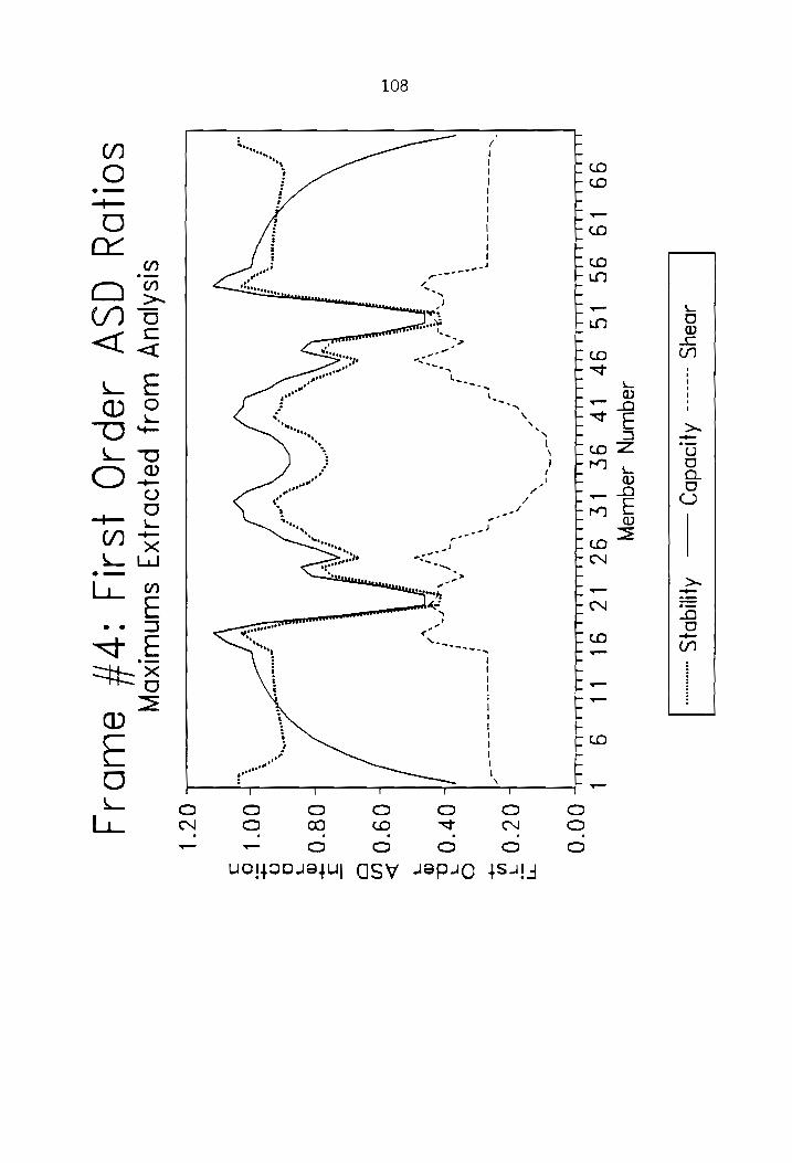
108
dpayg -------
Ayoodoy ——
Ayiiqoys
JOQLUINN Jaquuay
99 19
96 1G
OV IF
GE IE GO
te Gb
Vl G9
| Li bi tite ete tet
ee ete teed
et Eee yen
es tp
eat
pee
t eae
eee ta th
f~7
“=
¢ N
7 4
‘“
f ‘
, \
. f
s va
ae oe
~ Nn
ane eee
—-—--4
r “a
7~--r
t '
4 ’
, .
t A
‘ ‘
“
‘ ‘
‘ af
: :
a seer
ee eee a
Xs
An
\2
‘oo fy
\ 3
/ 5
\, \y
ix
. 7
‘ ‘y
‘, *
v \
‘ :
x x
e%
7:
EAX it
“2 yet
< so”
-
-
~
2
~ é
¥ :
. :
. f
. :
5 :
pitas
> “eee,
/
* ee fo
eee
moe PTA
etna seesane ~ 7
‘e _
S materemeeee “
* =
*
.
; 2
3 f
: -
~ 2
3
3
f *
.
00°0
FOC 0
F OVO
F090
- O80
Lb 00}
Oc |
SISAJOUW LUOJ}
PayoD4Xy SLUNLWIXD
SOHDY QSV
48P4Q 4S4l4
iyi eWDA44
}OD494U] QSY 48P4C 4S4l4 UO!

109
44] -------
d\GSY¥ ——
OS\CSV sm
JIQUINN JaquUay
99 19
9S 1G
9F Ih
9F IE 92
Ie
GEL G9
| Peder
t Pett
eee te
et pp
et tp ta Pt
Et
Et
T
a)
af ©
sjpsodoig Wod}
pejopsyxq SLUNWIXDW
SONDY AfIIGDS
pf SUDA 4
fo wo
Ud!I}OD 48ju| GSY 4EP4Q 4S4l4 JO S|dyiNW

110
99
Gad
------ d\GSV¥
—— OS\CSV
J8QLUNN Jaquuay\
19 99
1G 9V
Ih BY
IE YS
Le Jt
|b Y
l Litidr
ti t_itptpe
et ipee
tet tr rit
deer
td erat
etd
tt pee ett
at at t
h
tt
F x
Y “
a
. ee
4
pede
ee ne eetemmemartomensomemaneneememene mised
2 lime Sees,
i
ae
Lee
~
wf tye
t ay
"Senay .
' *
yee?
. '
\ i
\, f
y f
\ **Mimees,
.
one? |
' ‘
i '
: \
™
——
oy
' \
, t
—_-
a“ “Noe
‘ A
17
~ vn
“
‘a \
‘ Vert
8 ;
‘ ~~
AY
/ ‘
v 1
’ '
' v
N“N t
‘ —
‘ '
} '
’ .
‘ i
‘ i
' ;
‘ ‘
‘ \
‘ }
1 )
[ 4
' 4
6 ’
v
' ’
' ’
’ \
¢ t
' ’
‘ i
’ '
t ?
\ t
‘ .
' ‘
—
’ '
' ‘
t ‘
; 1
? ‘
t
4 '
' t
! '
’ ‘
1 t
' ’
, t
4 ‘
' ’
' »
9 toy
}
1 )
‘4 '
' y!
t '
‘ 5s
i J
Lt ‘
‘ +
‘ 1
( ’
' '
f '
‘ (
t '
1 th
' '
’ 4
1 ‘
; ‘
‘ '
t ‘
’ i
sjosodoug WOd}
payoo4lxy sluNWUIXDW
SOWDy Ajlopdpy)
:p# ewiD 4
06°0
OO'l
|
OC |
OF}
OV |
OSI
UOH}ID4B4U] GSY 48PAC 48414 4O ajdyINW

111
ADBUG ------ ~
AptODAOD ——
ANDY S
esrsrsra
JIQLUNN Jaquuayy
SL £9
19 GG
6h Fb
LE IE
GE 6b
Eb Z£
| PELLNETPEELE
PE)
te tet ha
tt
tt EE
a et
tah OL
O
nN
in ’
‘ ,
‘ )
7 '
‘ fr?
ON ‘A
. .
Ns ’
‘ n
OZ
Q
on "
—
fe J
\ i
a4 /
‘\ oe
te /
‘ at
. my
r ’
‘ A
te O¢g
0
ts
NN ”
—
' ~
i -~
ft .
7 ‘
- eo.
; '
if ~,
I Vv
v \
f ‘
pot ot
tr” Ve
~’ cn
poy
pe if
N\ row
“ey cy ‘Nt
° rr
3 ‘ ro
ve ’
‘
1 -- 74
P -_-—
y v
=, rz
v \
_-—
+ OS'0 + 09'0
| -OL°0
f ¥
- O80
hs bn
pent aa
: A
4
+ 060
wd wer"
“7 Lag
Fr Ol}
*Sueeseny
UOl}OD4B4U| GSY 48P4O 48414
Oc}
SISA|DUW LUOU
PaloD4LX SLUNLWIXDY\
SOHUDY GSY
4eP4Q 4S4l4
iG SUID. 4

112
O41 -------
d\GSV¥ ——
OS\SV
-
JOQUINN Jsquuayy
Fi L9
19 GS
64 Sr
LE IE
Ge 6b
Fl L£
| LUVPQEDLELDLELLILDALIT
LIED ILPIVEDLELELLILILL EP
Pet ee
Et ED Et
et Pt tht
a ta
O/'0
~
> ere oe
T
iw) ™
©
- 080 S80 - 060
‘L G60 lem SOs
ONY ws
flout
O21
JOD 4ajU] GSV 48P4O 4S4ly 4O s|dyiNW
udol
sjpsodoug WoOu}
payoo4lxy suunwuixoyp
SONDY ALIGDIS
:G# eluDI4
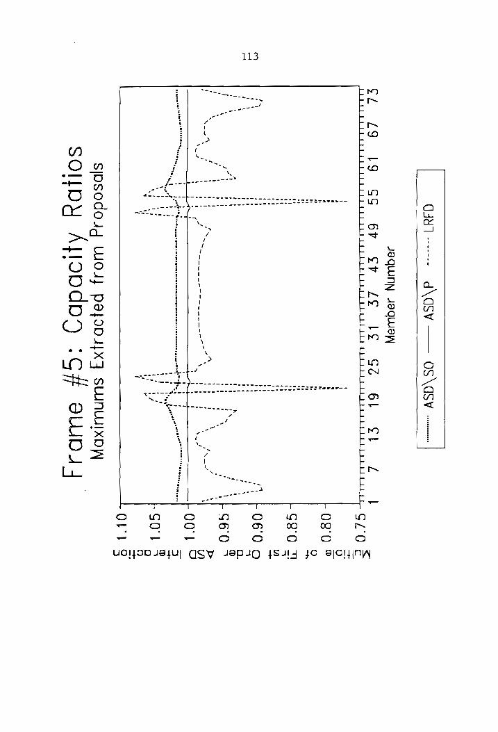
113
G447 -------
d\GS¥ ——
OS\CSV sm
JEQUINN JIquiayy
Si £9
19 GS
6
Sh LE
IE Ge
6b Ft
ZL |
PL LIE PELE Pte
tet
te tei
te dat
ea Peep tae eda reat et
th a
GL£Q
t '
1 J
’ 4
t 8
» t
a 4
u he
a "
te te
a 1
te 4a
or a)
ts te
eq t
ta oe
et "4
is Ye
ot ef
t '
vu ‘
’ rs.
ta '
' 7%
m4
4 4
» ¢
fos
a a)
, !
oy ‘ft
*4
' ‘
: ‘
' '
te ,
‘
4 4
ae i
h '
t ‘
‘ 7?
mA
an 1\
‘ }
‘ yr”
i
ba mes
/ 1
\ ’
4 4
ot :
‘ ?
t '
‘ t
' po
toe i
‘ '
:
‘ \
! '
sot m4
: \
J 1
‘ .-%
‘ '
' 1
os
vn
' '
‘ \
to ‘
‘ ~
‘ )
’ to
‘ wee
—
“77
\ tos
’ ‘
/ 7
‘ Nes
\ Bg
N ©
4 ‘
Ve
4 4
4 '
’ ak
t s
1-1
TT —
4 A
peat eseeeceem oa,
t '
‘ ‘
' '
' '
srr teM rears
seeeceeme” wer mee
' yon
Goss tecseent
os teressrede™
¢:.!
§ wee
Se mr
mewes
Tab ue
| PoP
pane ay
1 '
an |
Wegghl”
\
‘ \
‘ \
| '
}
1!
’ ‘
' vt
‘ }
0 !
' /
Yow
OF '
' ‘
(
- O80
- S80
- S60
T
©
cS
- GO|
sjposodoug Wod}
pepoo4yxqZ stunuuixow
soilpy Ajlondoy
:G# etups4
©
Udl}SD4ajuU] GSV 48p4O 4S4l4 4O SICHINW

114
ADU
------ ~ Ayyoodpy
——— Af IIQDYS
ase
JIQUNN JEquia,)
19 GS
6r Cr
¢e tE
Ge 6
Fh i
4
Libitittrpeptit
tt tart ryt
tttrertsieti
pets
ped tp
ett peepee
tt ta
a tt tt
O0'O
4 L O70
-0F'0 + 09'0 - 080 / 00°! 021 Or" 09" + 08" 002
sisAjouy WO}
pajop4lxy SLUNLWIXDW
SOHDY QSV
4eP4O fS4l4
:Q# SWI;
UOI}OD4BjU] GSY 48P4O 4Sul4

115
441 -------
d\dS¥ ——
OS\CSV
JBQLUuNN JequUUuay\
19 GS
6rh bv
¢e IE
Ge 6h
| l
| Litt tptttt
bpp
ttt
Perret
dp dete
tp
pp pe pate
ee et
tte tt
aa
1 pdt
t tpt
ft ti
Or
'O
sjpsodoig Wod}
pejop4yxq suunuIxDy
SOIMDY ALIIGDIS
:9f# aluDI4
UO!I}OD 4B}L| GSY 48P4O 4S4!4 40 SICHINA

116
G4y1 -------
d\GS¥ ——
OS\dSVv
JIQUINN Jaquuay\
19 GS
6” Sr
Le 46
Ge 6b
FI l
| LiitbbhLit
ppepditiytidr
ded pidtpetieti
tt
pri
ppp
tr titi
ts spit
id pitt
tt pt
a 060
_— — Teeter
rds Shh WT
* “
Tre ~~
we
* we
ra
‘ ‘ “4
“Seq .
te seeee
praceneseee®
may
pensemareere ness
eens get
: ‘
i ,
ay gdBOTmePeeT@trvegng,
oe
Teateseereee
as
= et’
! VoL
. “a
oF we
! 2
co '
‘ f
/ \
’ ‘
, A
' t
¢ ‘
' ’
/ \ ‘
A i
‘ A
an
' \
tay Js
A PY
, ro
1 ‘
1 ‘
\ "\
¢ '
t ‘
j x
‘
, pe
“7 /
\ 3
‘ !
\ rae
a
~ \
-~ ’
‘ ‘
‘ ¢
Le
re
ON 7
v! fof
; v
\ ’
‘, \
' ~
\ '
‘ f
‘ft vf
\ !
' ‘
' !
tu x
' ‘
' ’
' q
. ‘
! ‘
; \
' \
/ ‘
i ’
! ‘
' ‘
‘ ‘
: ’
‘ ‘
i \
! ’
U 1
4 i
i 1
J ‘
t .
? »
3 ‘
‘ sf
i!
’ '
' s
’ ‘
‘ '
‘ot
. J
t \
; 1
is rf
' ‘
Y
"4
s! Ve
‘ '
i! !
’ ‘
? if
e
1001
HOLL
- OZ)
L Ooh
L Or
LOS‘
LOSI
LOLI
UO!}OD J984U| GSY 48P4O 4S4l4 yO aidiyiNW
08}
sjpsodoig Wod}
payop4xq SlUNLUIXD)\
sOWpY Ajlopdoy)
:Q# aLluiDi 4

117
ADYS -------
Ayjopdpg ——
AyIqD4s
JIQUINN JEquay
v9 LS
OS oP
9¢ 62
CC Pitt
t pet
pt tt
pet peter
tte i ditt
a tt
peepee ete
pepe pt
te ta
lt
a tl
th
at
Gl 8
|
- r \
“A ’
‘\ 1
4 r
4 fd
‘ ’
4 ’
‘ ,
' ?
Y ’
1
i 4
r? ‘5
fos
a '
' ‘
Ln
r
uA a
! \
r J
\
Ta
_ (
‘ '
; roa
’ ‘
‘ ‘
\ !
‘ ‘
\ J
1 )
' ’
\ ’
’ ‘
’ \
' rT
' ’:
‘ ’
‘ t
s A
’ L
) ‘
r7
‘ t
- ’
’ ‘ee
\ !
\t \
A 1
‘ }
ve ‘
4K ’
a “s
. ’
x t
’ “
——
' ,
XY —~
,
'
N v
\ '
~ ‘
, at
% >
Set bEO
why =
t 4
y
Zz =
3
s e
e «
We?
i =
2 “ne
Fy .
* af
Thee -
:
é 4
00°0
- O60
-} OVO
{090
i+ 08°0
OO}
F Od}
SISAjDUW LUO}
pajoD4}xXqZ SLUNLWIXDY\
Or |
SOUDY GSV
4eP4Q fS4l4
Lf SwWDs;
UOIJOD 4ByU] GSY 48PsQ {S414
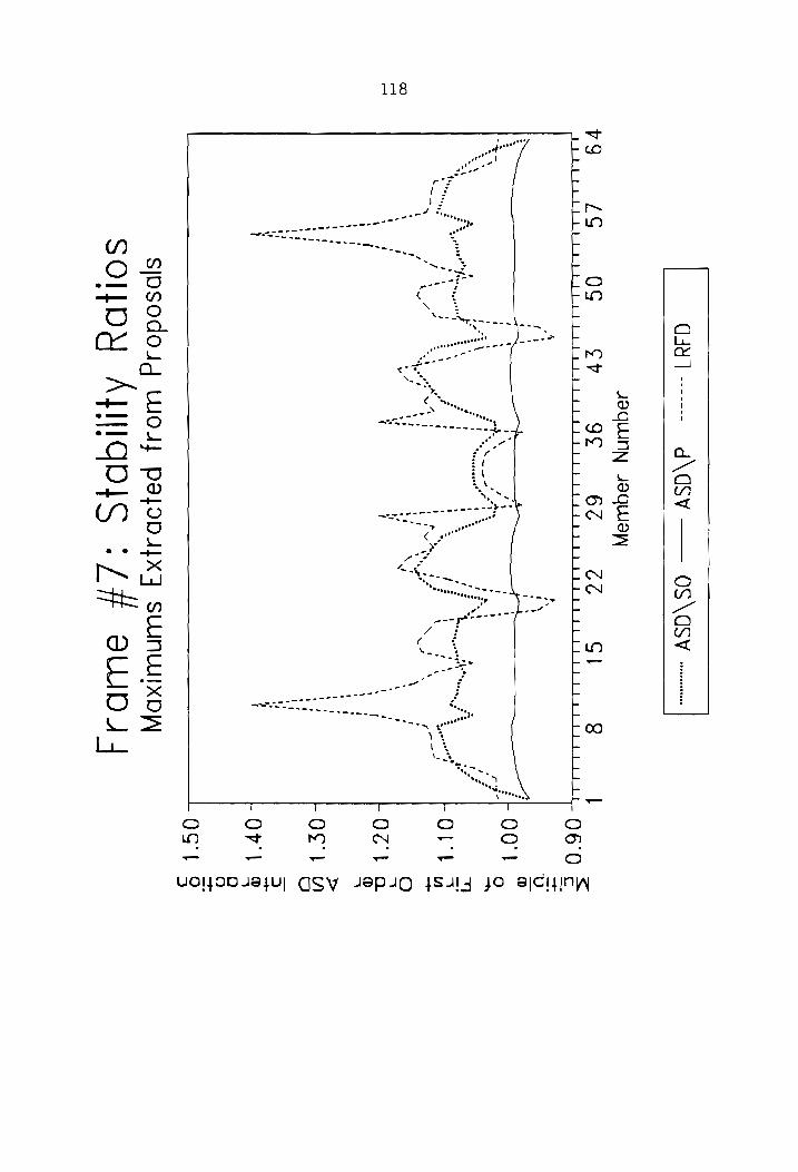
118
Q4u1 ------ -
d\agSv ——
OS\dSV
oocaeeeeeeenn
JOQUINN 4aquey—
v9 LS
OS cv
9¢ 62
GC Gl
PEtittiiett
pp apt tt
pet pt
te a tt
a at
8 |
LtLitieftet
ty
A \
fy
py
t 4
.
+ 14
'
3 t
l ‘
' 2
ro ,
/3
f :
- x"
' ‘
oh,
\ sae
' ’
c7
. \
' ‘
Fae
“ Ves
pay
a
> sy
Oy TA
paves
if
= .
, ed
- 4
Secenewese ,
' “
yo
Ms a
2 te
TAA x
ahah f
\ ft
' ;
*
Pers 3
‘, e
Fe gente
Pea
jeeeed ,
fo!
’ 3
tea eeeree
Mea FS
“ ts,
os '
2) :
i 4
1: ‘
ay ete
‘ “aye
a 8
t ‘
e
' t
Ln i:
eo See!
’ 7°
Z ‘
wy
1,
* 3
A ’
_-
“~ ’
\ ~
’ {
2 \
{ -
N
+ A
4
ae
Ww ’
’ a!
vw ta
Zs fa
4 é
~
\s’ f
, ty
vs Vv
:
' ,
vy
i? v2
‘ §
‘ ’
v ¢
.? af
sf '
‘ 3
i/ ?
d t
‘ it
? '
¥ §
{ {
t .
of ‘
| ar
t i
' ‘
4 '
' '
1 f
, 3
1 '
» ?
. rt
! '
i!
1 f
» é
i! vy
7 '
‘ é
i} My
s ,
rad r
1 i
' 4
‘ i!
} ’
060
f‘LOO'U
- Olt
- Od |
F OF}
- OF |
sjpsodoug Wod}
papod4lxXy SLUNLWIXDW
SONDY ALIGDIS
:/# auD44
oO a
UOI}SD 4ajuU| GSV 48p4O 4S4!4 4O siCyINA

119
G41 ------
— d\GS¥ ——
OS\CSV ws
JOQLUNN JaquuEW
¥9 LS
QS cP
9f 62
GC GI
8 |
DEtte_te_pteptet ype
petbpetpep ppp petpepeptete
perp ar tperititrirpiprrrtrrtritiptripitrirt
060
=
ry
oy
=
ty ‘
e
reAN /
’ s G6
0
' \
b 4
f 1
' \
“ ‘
° ’
\ ~
‘ 1
} \
O
we
Roverrwenserefoay, getter
etna,
3 t
peeengeeeeem tay,
wepteetesenenall
oe,
Q 0
| =,
teguent?
wey
r i
‘
J
i i
"
2
a
' ‘ rere
Soret
ea
| oN)
pe Ne
yee
yo _
’ ‘
—e
“cy
: \
Lv? \
| i
, ne
; '
ys
r~ GO
| ~y
f
‘ /
Lw
\ '
' '
~-
’ ;
, W
1 1
’ ‘
i ‘
§ ‘
i \
_—-
4 ‘
x e
ro ,
4 1}
i ,
4 ,
FOL }
’ ;
‘ ‘
' '
‘ ,
‘ O
’ ‘
i ’
' vy
' }
\ nN
i \
’ ot
t) ‘
‘ °
7 ;
' ’
; ‘
; ’
; 1
— G
| l
QO
5 ‘
,
' '
' 1
eH] ;
i I
’ !
{ ;
\ '
‘ “y
' ‘
} "
‘A
t '
' .
ia i
iH ti
ip OGh
p it
: ‘
‘i UV)
' ¢
. ;
; .
t !
‘ ‘
' it
G 6
| O
7 i
—_— *
: 3
aa
' .
vi 1
FOL
& VW ve
u
A
¥
2
HGS} Q —
, O
Or Q
SIDSOdoug WOd}
payoD4Xq SLUNLWIXDW
SOHWDY AJIODdD)
:/# alwiD44

120
O01
ADIYS -------
Ayooddg ——
Ajiiqoys
JIQLUNN JaquUay;
16 ¢€8
¢fL +9
GS 9F
LE 82
61 LEL
DAIL TEP TEEE
TIRE
E AEE T
EE
EE
ER EE
tt
Ol |
mv s
as fy
’ eoNL
a
1 i
ine
' +
' t
'’ Nn
' See
I ‘
; 1
' ’
1 t
Y a
’ ‘
\
4 ‘
‘ '
{ ’
1 ‘
' vA
al ’
‘ +
AN :
Vue -
ey mv!
- !
rev
‘ wot
wed
‘ 74
~ vd
, 4
) v
’ '
¢ ‘
; 1
A I
Vy
y ’
t 2
‘ ry
: ul
4 '
‘ nm
\ fu
‘ 1
No ~
or ~.
oA
‘
. n~
A '
vt t
‘
. 3 =
a at
e
2 :
e
3 : : :
i i
: :
~ i
; *,
2 6
oe ‘
3 :
= .
2 a
- ¢
2 3
. 2
.
.
$ me
Q0°0
- O2'0
-~ QF 0
~0O9'0
- 08°0
7+ 004
FOC |
SISA|DUW LUOU
palODUIXF SLUNLWIXDY\
OV}
SOHNDY GSV
4JOp4o 4S4l4
i Qy# ew 4
QSV 48P40 4{S84!4 UOIJOD J8}Ul

121
G44] -------
d\dSv¥ ——
OS\dSV =
JIQUINN JIqUay\
OOl 46
¢€8 ¢L
%¥79 GS
9
LE BE
61 OI
| LEP
TEL ERE LTE
P EPAPER TEE EE
I
ha
Or'o
~t oO ©
Oo
‘L O80
- 00°}
LOZ |
-H OVI
-
Oo oO oe = —_
sjpsodoig WOs}
papyop4xq SLUNLWIXDW
SONDY AfIIGDIS
:Q#f SUD,
UDH}SO4BjU] SY JEP4O 48414 JO siCHINW

122
G4u1
------- d\OGS¥V
——
OS\dSV -
JOQUINN JIquiayy
OOlL 16
¢é8 ¢fL
¥9 GG
9
LF BE
61 OD
| LXE
TEP EREEELP APLAR
TEVA
EE EE
A EEE
7 O60
c vo
—
=;
1 A
Ny
i :
a An
Loo ye
a
,ocoeenen Peete
TR eee,
r
‘ ‘
z pene
ee
ony, ON
, wD
eeeeps ane
\ weg n
ett?
' aoe
wes
' so’
‘ 4
“Sere
atten
2 N
qeteuet¥ag, 2
t uw
’ ‘
a
1 yee
et
5 :
were "
: \eH
1
i ‘
* '
af ’
ran
ees 3
O
° 7
‘ 1
; ‘
' ‘
4 .
¢ v7
' {
) '
Vs
‘ LOL
| >
" ‘
Vv !
, \
i Vv!
‘ i!
" ’
' 7N
' ‘
ws
' \
| ry
" i?
o\ .
fp ON
| 7
> '
’ \
' ‘
} t
; .
mo ,f
NG be
4G 1
pOChy
rho ye
he ae
+ Mt
: |
vi ty
\! \
mt 1?
, i!
r!
M4 ta
. pio
Y v4
"i y
+ Of
- OF
| O
_
' :
‘ '
4
iON prof
; i!
,ore
mo” QO
poN ta
i i!
Vt
os VL
op y
8 PoE?
ft i
Vr be
AR 5
; “A
Ne !
" a
a
‘ ;
‘ ‘J
4 i
‘- ‘
‘ >
‘LOGI W O
' ‘
—
\ .
' rh
»
© i
1 OLL
a ‘
wt Q
! o
Os!
g J
sjpsodoug Wod}
payonsyxy SLUNWIXDW
Ssollpy Ajlopdoy
:Qf# atlups4

123
ADOUG ------ ~
AptOO GD ———
AY IQ YS
ssnsesern
JBQUINN Jaquoy)
9°l béb
901 16
QL 19
9f 1g
9} |
LEAL PE
UATE PETE PEARED
DARD PP PEE EP
0
QO . QO
r
1%
, 4
ry S
\ i
. “F
02'0
- OF'0
- 09°0
iL ogo
JOD 494] GSV 48PsO 4Sul4
+ 00"!
uol
Loz
Or’) SISAJOUY
LUOJ} paloDsyxq
SLUNLUIXDW
SOUDY GSV
4eP4Q 4S4l4
:6# Stud,

124
aiy ----
d\GSV
——
OS\OSW wn
JOQLUNN JBQLUa\
9b
Leb 9Ol
L6 Lg
9V Le
9| |
-a~
' 4 ' ' ' ' ( ' ' ' ey
74
1
' \Jos
z 3
a $y
NS A
S ns
* ~
’ a,‘
. a
, ,
A
wi
wr ve
Nwte.
FA,
a” s
309"
Sea
et,
See
‘ wry
é
{4s {
’ {
’ a
. 4
’ Ve
\ r
,?
‘ Vio 0
' “
y/
v
LEER TEER R
EE
MALAI
QO Y
° O
! | O8'0
: i
Loot AL
Uf Pe ety
pooner spe
po yas
Oc |
on ; 7
r
, ow
vy
LOP'l
:4 af -
O90
UOl}DO 4B}U] GSY 4EP4C 48414 JO sidiyiny
Oo co
sjpsodoig WoO}
papoo4lxq sLuNUIXDW
SONDY ApIGDIS
:G6 7 eluDs4

125
G4u] -------
d\GS¥ ——
OS\OSV w--
JBQLUNN JEquay\
9Fb Lol
901 16
QL L9
OY Lg
9I PUTED
—
4 3
hee
/~ an
fm
' ,
oN {
‘ ;
\ ra AT
‘. i
: !
vam,
! '
‘ \
f ’
\ 3
‘oe v
\ !
‘
; i
4g yf
‘ '
} ‘
PG
We ae
Vik
' a
*®
= pene
neeeenereeen beret
/ O01 tear gfemwenes ee en aenee
anal
“A
ue
oe
"A wd ecemeee sPatenPhceem eet
t ‘
AS
4 J
a] ‘}
{ '
fn
Mo
ty, te
vs :
t oa
x
| '
ve t
‘7 1
’ \
; \
“ve “
v Fiat
y \
7 '
vA
|
ro vy
% r
\ v/
N /
wo
‘ -
+ QO'¢ oOo Co
fOD4S}U| CSV 48P4O 4S4ly 40 BjCyiny
—
© © oO ©
-OV't
-Q9't
- O81
uol
O0¢
sjpsodoug Wod}
pejop4yxq stunuixoyp)
SONUDY AjloDdDy)
:6f# elups4

126
ADBUS ------ -
ApyODAD ——
— APIQDYS onsen
JBQUINN Jaques;
19 9G
1S QF
Irv 9F
IE 96
16 9E
th
GQ St
Litisyrtrsetrp eer
pit
teria ttp tity
tp aebtetertetprrtrterts pet ppt
tae tetpppt
tsp petit
orem)
- O20
oar”
LOr'O
L990
Lago
elem!
FOC |
Or} SISAIDUY
LUO} PaLoD4LxXy
SLUNLUIXDY\
SOHDY GSV
4eP4O JS4l4
‘OL # suiD44
UOl}9D484}U] GSY 48P4O 4Su4l4

127
G4Y7 ------
d\GS¥ ——
OS\CSY
JOQUINN Jaquuay)
19 9G
IS OF
Ih 9F
IE GE
Ie GE
Fl YQ
tiddia
ttt ttt
pe tt
bt pp tt
et a
aa ht
a
at a
|
Or 0
+ 09°0
7L O80
00°!
LOZ I
a!
L09'|
Og"
00°¢
sjpsodoug Wod}
pajop4jxq slunuuixoyw
SONDY AfIIGDIS
:O) #
SWI;
UOI}OD J84U] GSY 4EPIQ 48414 JO SICIINY

128
Q4u]
------ - d\agsSv¥
——
OS\dSV
JOQLUNN JOqLUa)\
19 9S
1G 9”
Ih 9F
IE 9
12 9
th GQ
| LLit
dp ti
pete
te tad pete t
att tee
et itep
ts pete
eet
a tt
pete
tp pet
ttt tea
a a OV 0
: i .
: :
: :
: 3
3 ry
ry :
+ “
—!"
a +
. ne
‘ '
‘LU?
' r
. ws
\ {
‘ r
ia meee,
: '
A. tS,
? wae
t one
‘
’ ‘son
Sates omens
. oo
teeny }
1 amnneees
ee
‘ f
XN ome
* “sete, eeqncentettesey aveeste
CURE
TT | seecresgtt
o
Vsete Aide?
. /
}
‘ se
‘ \
i !
‘ ‘\
- a”
‘ ¢
‘ (
‘ ‘
ne
/
‘ i
i '
. >
“ :
’ w
1 ¢
’ Ui
- ’
s ‘
' ’
, ‘
! ‘
0 4
f (
‘ ‘
' i
a ‘
} \
’ e
{ '
’ ’
1 '
, ‘
( \
t '
! i
: ‘
é ’
~
’ ;
o~— OY
t ’
cr “eh
' .
7
' t
' ‘
“N !
' t
v 1
’ '
, N
\ '
\ t
' ’
‘ '
‘ '
nr) ‘
, ‘
‘ t
xf ‘
/ '
_ i"
7+ 09°0
- O80
- QO'1
- Od |}
- QV |
o ©
sjpsodoug Wood}
pajopsyxy SLuNWIxDy)\
soupy ALiopdoy
:o|,# elup43
UOHOD4B4U| GSY 48P4Q 48414 JO aidiyiny

APPENDIX B
BEAM-COLUMN DIFFERENTIAL EQUATION DERIVATION
129

130
Differential Equation Derivation
1. Beam—Column w/ Transverse Loading
p a P
3. Axial Force Influence
pix
44 P
Le— dx —e
Figure B.1
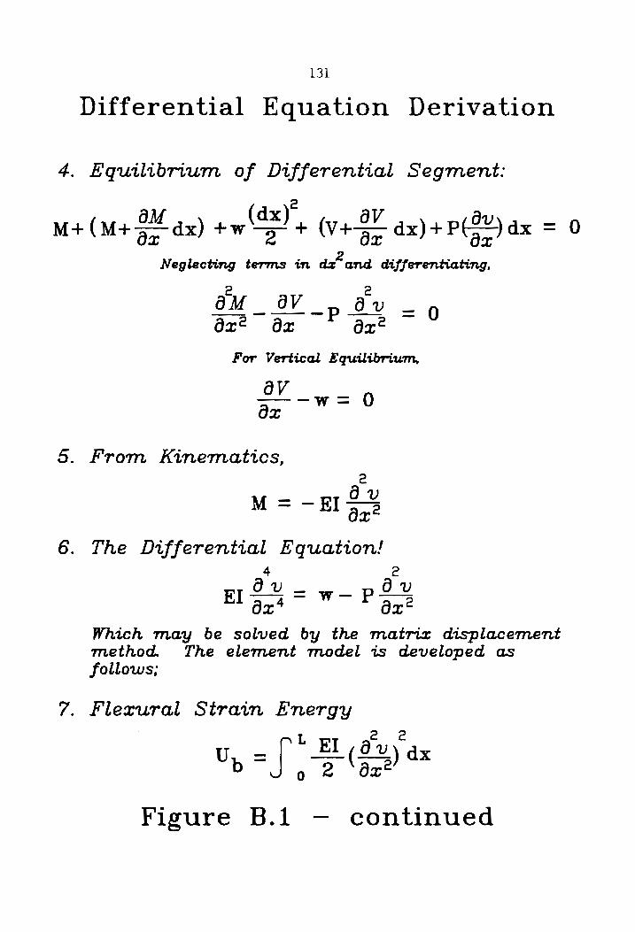
131
Differential Equation Derivation
4. Equilibrium of Differential Segment.
2 dx
M+(M+244 ax ) +w 4 (ve dx )+ PY) dx = 0
Neglecting terms in wont differentiating,
2
ax® Ox Ax*
For Vertical Equilibrium,
OV ax w= 0
5. From Kinematics, 2
—~ _p Ov M = —E] axe
6. The Differential Equation! 4 2
Ov — Ov Blg,4- © P Ax®
Which may be solved by the matriz displacement method. The element model is developed as follows;
7. Flexural Strain energy
U dx b~J, Y HL (uy
Figure B.1l — continued

132
Differential Equation Derivation
8. Solution of Equation
Neglecting the azial force, the beam solution is
5! Vv — 0
dx*
v(x) = at+axtart ax”
9. Selecting Nodal Displacements,
v(x) = f(xz)u+f(x)O+ f(x)ur+f(x)o,
e 3 99 ’
oe = £( x Ju+ f( x JO+ £( x Jus fl x }0,
Q
The influence coefficients are found by
kj = EI flz)f(x)ax ol j
Notes: 1.Neglects Axial Deformation and Second-Order Effects Z2.4f} is determined from the Element Boundary Conditions
Coefficients az are matched to Nodal DOFs to form the required Shape Functions jf}.
10. Modification for Beam—Column
To account for second-order effects, the influence of the axial load on the bending stiffness coefficients is determined by factoring the flexural stiffness coefficients (derived above) by the phi (>) factors shown in Chapter III (derived from the Stability Functions).
Figure B.1 — continued

APPENDIX C
TAPERED MEMBER CONVERGENCE STUDY
C.1 Beam Behavior
Obviously, a stepped beam analysis is an approximate estimate of the
continuum mode! of the tapered beam. Although first-order elastic analysis
does not require iteration, this application of the displacement method is
technically a convergence problem. The use of a stepped beam model is a
transition from the realm of the matrix displacement method (MDM) into the
world of finite element analysis (FEA). As a consequence of discretization,
error in analysis of the displacements is introduced. The magnitude of these
errors depends on the similitude of the model and the continuum.
The more elements that are used in the analysis, the closer to the exact
solution. However, as the number of elements increases, so does the time
required to perform the analysis. A typical tapered beam is studied in Table
C.1. This example is taken from Yang (1986). This tapered cantilever shows
that eight uniform elements were required to reduce the error in the tip
displacements to below 1%. Consequently, the error is less than 1% using
only two tapered elements. The exact solution may be converged upon by
selecting a higher degree of freedom discretization, as Table C.1 indicates.
This convergence process is known as monotonic convergence from below.
If a plot was constructed with a displacement as the vertical axis and the
number of elements as the horizontal axis, the exact solution would be
133

134
Error Analysis of Uniform Element Approach to Tapered Beam
lo
Uniform Elements
Parameters
o
Yr
1 8
Tapered Elements
Error in Tip | Error in Tip| Error in Tip|Error in Tip
Number of Deflection Slope Deflection Slope
Elements (%) (%) (%) (%)
1 30.30 10.29 —0.62 2.82 2 8.58 5.04 —0.17 0.77 3 3.92 2.99 4 2.22 1.97 6 0.98 1.02 8 0.55 0.62 12 0.24 0.30 16 0.14 0.17
Table C.1

135
approached asymptotically as the chosen number of degrees of freedom
increases. Such a graph is presented later. This can be explained by the fact
that in an FEA, the model always possesses a greater degree of stiffness than
the continuum, because of the discretization.
The NUCOR software used for analysis and design of rigid frames
generally specifies a joint or nodal coordinate every 2.5 ft. For a tapered beam
of length 20 ft., this results in eight elements for the discretization. By Yang’s
analysis, the analysis should possess a maximum error under one percent. A
positive value of the percent error signifies that the displacement has been
underestimated.
C.2 Beam-Column Behavior
A typical NUCOR beam-column has a taper ratio (7) of 3.0, and a
vertical height of 30 ft (7 = (depth of larger end - depth of smaller end)/depth
of smaller end). It also possesses representative cross-sectional dimensions
of a 12 in. depth at the base, flange widths and thicknesses of 6.0 in. and 0.25
in. respectively, and a web thickness of 0.2060 in. The ratio of the larger end
moment of inertia to that of the smaller end is approximately twelve. These
dimensions were selected to represent the type of construction normally used
by NUCOR frames. The boundary conditions were selected to maximize
errors in the analysis, as the free end is subjected to a vertical and horizontal
load and the larger end is fixed. The loads are typical to a combination case of
dead and snow loads. Though these boundary conditions are not
representative of NUCOR frame construction (an individual fix/free column),
the errors involved in a frame analysis should be of the same order. ANUCOR
beam-column would have the smaller end pinned (allowing rotation but no

136
displacement), and the larger end rigidly connected to a rafter (allowing both
rotation and displacement, but the angle between the column and rafter
remains unchanged). The analysis is performed using the proposed P-Delta
program developed in this study, and the results are shown in a form similar to
that of Yang, described above.
A NUCOR software discretization would have used approximately 30.0
ft / 2.5 ft/element = 12 elements. By Table C.2, the error in deformations at
the tip for lateral and rotational displacements would be on the order of 15%.
Correspondingly, for second-order elastic beam-column behavior, the same
discretization would also produce an error on the order of 15%. With this
amount of error in discretizations, stress calculations would be unconservative
by this same amount by first-order analysis. To obtain a solution with less than
1%, 128 elements would be required. Figure C.1 shows the convergence
study plots for this beam-column, for the tip-displacement and base moment.
Because of the discretization error, the NUCOR software should be called an
FEA program, not an MDM program.
For practical reasons, it is not recommended to model a tapered
column with a uniform element every six inches. What is recommended is that
the software use more elements than currently employed, and recognition of
the amount of error in the discretization process. This error is probably on the
order of 10%. The best recommendation is to utilize tapered elements instead
of uniform elements for the analysis. With tapered elements, the current
discretization could be held, and the accuracy of the results improved. Figure
C.2 (Galambos, 1976) could be used as a guide in the development of a

137
Tapered Beam—-Column Mocleling with Uniform Elements
d = 12’
b,= 6.0" t,= 0.25" tw= 0.2060”
—
d = 48
Convergence Study
B| | 717 Sf
First Order Analysis
Parameters
P = 30 kips Q= 6 kips
H = 30 ft
| Second Order Analysis
Error in Tip | Error in Tip| Error in Tip|Error in Tip
Number of Deflection Slope Deflection Slope
Elements (%) (%) (%) (%) 1 69.93 62.79 73.03 66.62 2 52.61 48.32 56.30 50.50 4 34.84 30.66 38.29 34.33 8 20.39 15.21 22.93 20.65 16 10.82 9.62 12.36 11.19 32 5.29 4.51 6.10 5.54 64 2.32 2.07 2.69 2.45 128 0.78 0.70 0.91 0.83
0.00 0.00 0.00 0.00 Table C.2
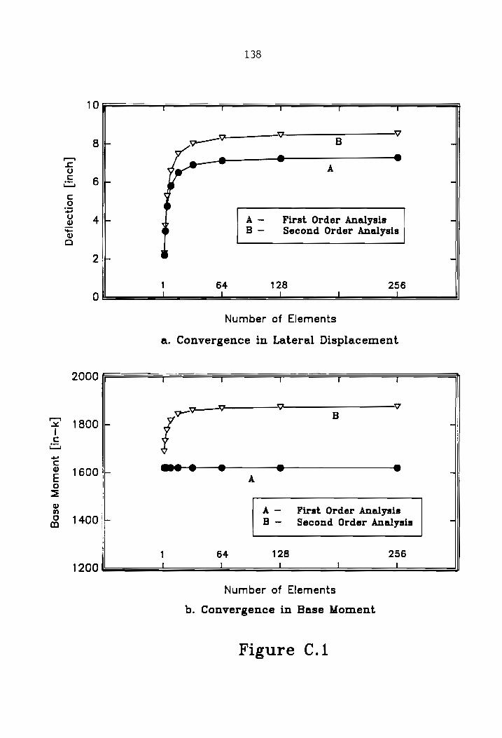
Base
Moment
[in—
k]
138
1 0 7 t I 1 r t
7 v Vv 8 7 B = ——_® ® s A
= 6 c 2
9 4 A- First Order Analysis 3 B- Second Order Analysis
a
Number of Elements
a. Convergence in Lateral Displacement
2000 -— =
1800
1600!
A -
B-
First Order Analysis
Second Order Analysis
1400: \
F
r 256 1 64 128
Number of Elements
i a
b. Convergence in Base Moment
Figure C.1

139
Sign Convention used in the following derivation;
Map CooL oor LoL Mba
Oba
Slope Deflection Equation for Tapered Members:
M,,L Mpa L Aab > Oav = EL. Oe “El, Cyt a + Oxb
M pL Moe L A 7
Onn Oba End Rotations of Tangents to the Elastic Curve
Opn Oba End Rotations of Tangents to the Elastic Curve for a Simply Supported Beam
Cij Unit Moment/Rotation Coefficients for Tapered Beam (functions of geometry and loading).
Tapered Beam—-Column Element
Figure C.2

140
a = ut m (1+7v)?
P — n°Elg n = (1+)
exo L?
1 a P= lf 77-73
y = F17do ‘ d
0 a 1 p= J 5-;
For: a/y® s 1/4
1 _ x mtn _1 Cae a 4(P mo 5)
Y 2p 1 Cop - Co. = a/1+y m-n "8
1 _ Y mtn 1
Cop a a(isy) ° m-n +3?
For: a / »* > 1/4
Y Cae - 7 2 Fees
Cap Cy. = a = Bese(B In(1+7))~
1
Tapered Beam—-Column Element
Figure C.2 — continued

141
tapered beam-column element, though there are other tapered element
models possible.
The frames that were studied in the research used the same
discretizations that NUCOR software had used. Therefore, the error in the
analysis results of the research are of the same order as originally introduced
by NUCOR.

APPENDIX D
SLENDER MEMBER DESIGN
D.1 Axial Capacity
D.1.1 General
The development of axial compressive strength for slender | cross-sections
depends on both the maximum slenderness ratio for overall buckling, and the
level of stress on the cross-section for local buckling. The AISC Specification
provisions governing axial capacity were borrowed from the 1968 AISI
Specification provisions for cold-formed steel design with some modifications.
The design equations for column strength in the 1968 AISI Specification, for load
determination analysis, are as follows:
For
C Ye KL/r < 76
_120R, 3(aF,)°(AS* Fa4 = 33 - 9 (D.1)
23n°E
For
Cc Ye KL/r < 76
120° Fay = (D.2) 23(Kj?
142

143
Where the Q form-factor is determined according to cross-section element
slenderness ratios, which establish the maximum allowable stresses to prevent a
local buckling failure before lateral buckling. This Q depends on whether the
cross-section has slender stiffened and/or unstiffened elements. These AISI
provisions form the basis of slender-cross-section design in the AISC
Specifications. Depending on whether ail or some elements of the cross-section
are slender, application of the AISC provisions results in replacing the full cross-
section with an effective cross-section.
D.1.2 Unstiffened Elements Slender Only
For unstiffened elements (e.g., the flanges of an I-shape), the AISC
provisions utilize a reduced average stress to account for softening due to local
buckling. By the 1978 ASD or 1986 LRFD Specification, the Qg factor reduces the
average stress, according to its slenderness ratio (b¢/2t-) and yield stress. By the
1989 ASD Specification, the Qs factor depends not only on the element
sienderness and yield stress, but also the web h/t ratio for a flange/web local
buckling interaction effect. The 1989 AISC ASD equations for Qs are as follows:
ke = —405 _ D.3 (r/10-46 (D.3)
_ Ds Qs = 1.293 - 0.00809 5 JFy/ke (D.4)
Qs = 26,200 ke (D5)
Fy(eLyy

144
These Qg factors are defined as the ratio of the local buckling strength to
the yield strength. This calculation is not iterative as it is not dependent on the
level of applied stress. The effect of this factor can be seen in Figure D.1a. An
example illustrating the effect on a cross-section when the unstiffened elements
are slender is provided below.
Example: Fa Calculation, 1989 AISC ASD Specification
Given Data;
KL/r = 45.0 A =5.5in@ Fy = SOQksi Cc = 107.0 be = 7 in te = 0.25 in Ne = 8in tw = 0.25 in
Table B5.1, pg. 5-36
Ae/tw = 32.0 < (253//50 = 35. 78) ; Noncompact Ne/tw = 32.0 < 70 ke = 1.0 be/2t¢ = 14.0 > ter a = 13.44) ;A/B, Qs < 1.0 bt/2te = 14.0 < (195//50 = 27.58) : Eqn’ A-B5-3
Appendix B
Qs = 1.293 - 0.00309(14.0)(7.07) = 0.9871 Qa = O. 6 (Web Noncompact)
= (0. S871 0) = 0.9871 C c= PeFQ S = 107.0//0.9871 = 107.7
Table 3, pg. 5-119
KL/rC’c = 0.4178 Ca = 0.503
Allowable Compressive Stress
Fe = CaQs QaF
= (0.503)(0.9871)(1.0)(50 ksi) = 24.83 ksi
Fa = 24.83 ksi
D.1.3 Stiffened Elements Slender Only
For stiffened elements (e.g., the web of an |I-shape), the AISC provisions
utilize an effective width concept. By the 1978, 1989 AISC ASD Specifications and

145
em Equivalent Reduction of Flange Area
Qa = 1.0 Qs < 1.0
a) Slender Unstiffened Elements
my Deducted Area
Qa < 1.0 Qs = 1.0
44.3
bp zest [1 - 7 Shee eff Jt
b) Slender Stiffened Elements
mi Deducted Area
Qa < 1.0 Qs < 1.0
c) Slender Unstiffened & Stiffened Elements
|
Reduction Factar Analysis Figure D.1.

146
the 1986 AISC LRFD Specification, the form-factor Qa modifies the cross-section
area according to the web slenderness ratio (h/ty) and the level of compression
stress considered. This Qg factor is defined as the ratio of the local buckling
strength to the yield strength. According to the 1968 AISI Specification, the stress
level used in computing the cross-section properties is the local buckling stress
of the unstiffened elements, QsFy. This is a conservative approach, and was not
adopted by the AISC. In ASD, a lower bound on the reduction in effective width is
set so that beff is not less than 253t//Fy. By the 1978 or 1989 AISC ASD
Specifications, the effective width of the stiffened element is determined from (with
a factor of safety of 1.66):
253 t betf = —— [1-44.93] (D.6)
if (b/t) /f and
253 t Minimum beft = (0.7) /Fy
where f = Fa. Since Fg is unknown initially, an assumption of 0.6Fy may be used
to obtain a lower bound on beg. Then, iterations are performed until bef and Fa
converge to a constant value.
By the 1986 AISC LRFD Specification (factor of safety is removed):
bet = oo tw py - 82.3 (0.8) it (b/tyst

147
where f = 6Pn/Ag- Since ¢Pp is unknown initially, an assumption of 0.85AgFy
may be used to obtain a lower bound on be#. Then, iterations are performed until
bet and ¢P, converge to a constant value.
In LRFD, their is no minimum be# specified. However, it is assumed
that LRFD intended to provide a minimum begf value. Logically, this value can be
assumed to be:
326 t yy
i Fy Minimum Deft = (D.9)
The effect of the Qg factor can be seen in Figure D.1b. The bef equation
shown is taken from the AISC ASD Specifications. The effective widths calculated
by this procedure are greater than those that would be obtained by directly
applying the AISI provisions, as the level of stress f used is not necessarily the
maximum level that can be applied to the unstiffened elements.
An example which illustrates the effective width concept when the stiffened
element is slender is provided below.
Example: Fa Calculation, 1989 AISC ASD Specification
Given Data;
KL/r = 45.0 A = 10.5in@ Fy = 50 ksi Cc = 107.0 bf = 6in tf = 0.375 in Ne = 24 in tw = 0.25 in
Table B5.1, pg. 5-36
No/tw = 96.0 > (253//50 = 35.78) ; Slender A/B Nc/tw = 96.0 > 70 ; Kg = 0.5663 b/2t¢ = 8.0 < (95//(50/k_) = 10.11) ; Noncompact
<< Iteration 1 >>

148
assume y= = 0.6FyQs = 0.6(50 ksi)(1.0) = 30 ksi = 10
batt = (253(.25)//30) [1-44.3/((86)/30)} = 10.57" Qa = (10.5-(24-10.57)( 25))/10.5 = 0.6802 Q'= O50a = (1.0(0-8802) = 0.6802
Cc C’c = Q = 107.0//0.6802 = 129.7 KL/rC’c = 45.0/129.7 = 0.3470 ca = 0.525 Fo = CaQs QsF
FS = (0.525)(1.0)(0.6802)(S0ksi) = 17.86 ksi < 30 ksi
< < Iteration 2 >>
Assume f = 17.86 ksi betf = (253(.25)//17.86) [1-44 3/(96/17.86)] = 13.33"
= (10.5-(24-13.98)(.25))/1 0.5 = 0.7460 = (1.0)(0.7460) = 0.7460
Gio = Seta = 107, 0//0.7460 = 123.9 KL/rC’c = 45.0/123.9 = 0.3632 Ca = 0.520 Fa >= CaQc,Q F
FS = (0.520)(1.0)(0.7460)(50ksi) = 19.40 ksi > 17.86 ksi
< < Iteration 3 >>
Assume f = 19.40 ksi bett = (253(.25)//19.40) [1-44.3/(96/19.40)] = 12.86" Qa = (10.5-(24-12.86)(25))/10.5 = 0.7348
= (1.0)(0.7348) = 0.7348 Cio = sae Say. 0//0.7348 = 124.8 KL/rC'c ='45.0/124.8 = 0.3606 va = 0.520 Fa = CaQs QaF
Fa = (0.520)(1.0)(0.7348)(50ksi) = 19.10 ksi ~ 19.40 ksi
Fa = 19.10 ksi
D.1.4 Unstiffened Slender and Stiffened Slender Elements
When the cross-section contains both unstiffened and stiffened slender
elements, the procedure is also iterative. The AISI provisions would apply the
maximum design stress in the unstiffened elements to the stiffened elements. In
this fashion, the AISI procedure would result in the web always possessing its
minimum available cross-section area. However, this is not the case by the AISC
procedure. By the AISC method the web cross-section area is greater, iterating

149
to locate the effective width of the web. The effect of both Qs and Qa factors on
the cross-section is shown in Figure D.1c. The allowable stress by this procedure
will be higher than that of the A/S! procedure, since the converged effective width
of the section will be higher than that found using the maximum level of stress in
the unstiffened elements.
It is reiterated here that the column allowable stress is not dependent on
the service load compressive stress, but the maximum level of stress that can be
applied to cause local buckling. The allowable compressive stress is determined
as though the member were a stand-alone column. This is true whether or not
the member is a column or a beam-column. The effective-length factor is still a
necessary entity, governing the overall column behavior. The column strength
should be developed independent of actual service load stress conditions. The
following example illustrates the procedure for column allowable stress when both
the flanges and web are slender.
Example: Fa Calculation, 1989 AISC ASD Specification
Given Data;
KL/r = 45.0 A = 10.5in@ Fy = 50ksi Cc = 107.0 bf = 7in t¢ = 0.25 in Ae = 24in tw = 0.25in
Table B5.1, pg. 5-36
Ne/tw = 96.0 > (253//50) = 35.78) ; Slender, Qa < 1.0 Nco/tw = 96.0 > 70.0 > ke = 0.5663 be/2t = 14.0 > (95//(50/k.) = 10.11); ‘Slender, Qs < 1.0 b/2tp = 14.0 < (195//(50/ke) = 20.75 ; Eqn. A-B5- 3
< < Iteration 1 >>

150
Qg = 1.293 - 0.00309(14.0)(9.40) = 0.8864 ee 0.70 (assumed)
= (0.8864)(0.70) = 0.6205 Assume f ~ O6E,0 = 0.6(60 ksi)(0.6205) = 18.62 ksi best = (253(.25)//18.62) (1-44.3/(96/18.62)] = 13.09" Ga = (10.5-(24-13.09)(25))/10.5 = 0.7402
= (0. 0.8864)(0 7402) = 0.6561 Cio = Bei/O © 107.6) /0.6861 = 1321 KL/rC’e = 45.0/132.1 = 0.3407 Ga = 0.527 Fa = CaQsQaF FS = (0.527)(0.8864) (0.6561)(S0ksi) = 15.32 ksi < 18.62 ksi
< < Iteration 2 >>
Assume f = 15.32 ksi Detf = (253(.25)//15.32) [1-44.3/(96/15.32)] = 14.25" Qs = as 5-(24-14.25)(.25))/10.5 = 0.7679 Q= = (0.8864) iy .7679) = 0.6807
O89 J Cc = Q = 107.0//0.6807 = 129.7 KL/rC’c = 45.0/129.7 = 0.3470 ca = 0.525 Fa = CaQF
Fa = (0.525\(0.6807)(S0ksi) = 17.87 ksi > 15.32 ksi
< < Iteration 3 >>
Assume f = 17.87 ksi Deft = (253(.25)//17.87) [1-44.3/(96/17.87)] = 13.33" Qa = te 5- -(24- -13.33)(.25))/10.5 = 0.7460 Q= = (0.8864) v .7460) = 0.6613 Cig = beta © 107.6) 06818 © 131 6 KL/rC’c = 45.0/131.6 = 0.3419 va = 0.526 Fa = CaQF
FS = (0.526\(0.6613)(50ksi) = 17.40 ksi ~ 17.87 ksi
Fa = 17.40 ksi
D.2 Flexural Capacity
By the 1978 or 1989 AISC ASD Specifications, the allowable flexural stress
of an |-shaped cross-section (when both the flanges and web are slender) is
developed as the minimum of 0.6FyQsg, or the plate girder allowable stress. The
effect of Qs on the cross-section was shown in Figure D.1a, and is not an iterative
process to determine. The 0.6FyQs (ASD) is applicable to prevent local buckling

151
of the compression flange, and is calculated as described above. When the web
h/t ratio exceeds 760//Fp, plate girder provisions apply (The 760//Fp limit may
be changed to 970//Fy (Iwankiw, 1990]). The plate girder provisions account for
bend buckling of the web, and the accompanying increased stress in the
compression flange, and are found Section 1.10.6 of the 1978 ASD Specification,
or Chapter G of the 1989 ASD Specification.
By the 1986 LRFD Specification, the flexural strength is also developed
according to the web slenderness ratio. If the flanges are slender, and the web
h/t ratio is less than 970//Fy, the provisions of Appendix F apply. Regardless of
whether or not the flanges are slender, if the web h/t ratio is greater than
970//Fy, the plate girder provisions of Appendix G apply. Appendix G directly
accounts for both lateral-torsional buckling and flange local buckling.
Application of the plate girder provisions of both ASD and LRFD has the
effect of replacing the original cross-section with an effective cross-section. This
effective cross-section results from bend buckling of the web. As the web buckles
in regions of high compressive stress and moves out-of-plane, the compression
flange receives the stress transfer. Rather than performing lengthy calculations to
obtain the effective cross-section properties for this condition, the AISC
Specifications use an equation to reduce the full section modulus to an effective
section modulus (the formula shows a reduction of the allowable bending stress,
but this is not what is really happening). This effect is shown in Figure D.2. In
ASD, the basic Fp used in the plate girder equation is selected from the lateral-
torsional buckling allowable stresses, or O0.6Fy, whichever is smaller. In LRFD, the
Critical buckling stress is developed according to the lateral-torsional buckling
strength, and the flange local buckling strength.

152
t [-— bp —=]
te | | 3 Deducted Area
he D N.A.—— # —— °
ASD Plate Girder Section Factor
R = 1 — 0.0005( =I we De an " A, ‘LV t.
LRFD Plate Girder Section Factor
A 970 h R= 1 — 0.0005( =) —— — ——
Pg A; V FY t,
Plate Girder Effective Section
Figure D.2

153
The flange local buckling (FLB) limits in the 1989 ASD Specification involve
the web h/t ratio, but the 1986 LRFD Specification FLB limits do not. This is the
reason for the economic envelope shown earlier in Figure 4.2. By the 1989 ASD
Specification, the allowable flexural stress must be selected as the minimum of the
plate girder and slender flange provisions, if applicable. Utilizing LRFD in the
range of 70 < h/t < 970//Fy, this condition can resuit in beams having flexural
strengths approximately twelve percent higher than the same cross-section by the
ASD Specification, including the load-effects side of the LRFD format equation.
The following example illustrates the calculation of the flexural allowable
stress on an I-shaped cross-section whose flanges are compact but the web is
slender.
Example: Fp Calculation, 1989 AISC ASD Specification
Given Data; Compression Flange Fully Braced
Fy = 50ksi Syo = 199.2 in? = 6in te = 0.375 in
Ac = 48 in tw = 0.25 in
Table B5.1, pg. 5-36
Assume Fp = 30 ksi No/tw = 192.0 > (760//30) = 138.8) ;C/Gor A/B Ao/tw = 192.0 > 70 ‘ke = 0.3607 by/2t = 8.0 < (95//(50/ke) = 8.07) ; Compact, C/G
Allowable Stress
Roa Fb = 30 ksi, as assumed above sea 0-0. 9.0008 (48*0. 25) /(6*0.375))(192.0-138.8) = 0.8581
Syc’ = = SEE 199.2in*3) = 170.93 in?

154
Fp = 30 ksi Syc’ = 170.93 in?
D.3 Beam-Column Interaction
As described earlier, the column allowable stress (ASD) or the column
capacity (LRFD) determined independently of service loading is utilized in the
interaction formulas. An omission in the 1978 ASD Specification, and now
appearing in the 1989 Specification, is the use of the combined form-factor Q
(Q=Qs5Qa) in the denominator of the axial term of the yielding equation. This
results in higher interaction values than with the 1978 ASD Specification. The
1989 ASD equation is as follows:
anor + Ps 1.0 (0.10)
As an example, if the form factor is 0.85, the axial term would become 1/0.85 =
1.18, or 18% higher than in the 1978 ASD. The increase in the interaction ratio is
lower, depending on the magnitude of the flexural term.
The allowable stresses (ASD) or the strengths (LRFD) calculated as though
the member was a column or a beam, respectively, are used in the interaction
equations. In other words, the denominators of the interaction equations are
independent of the applied loads, but the numerators vary according to actual
load combination effects.
The following example illustrates the difference between the 1978 and 1989
ASD Specification interaction equations.
Example: Interaction Ratios, AISC ASD Specifications

155
Given Data;
Unbraced Frame, First-Order Analysis & Design Fy = 50.0 ksi F’g = 60.0 ksi fg = 4.0ksi Fa = 16.0 ksi Q = 0.60 fh = 24.0 ksi Fr = 30.0 ksi
Stability: 1978 or 1989 ASD Specification
fa/Fa + Cm/(1-fa/F'e) (fp/Fb) £0/%6.0 + 0. Be ae 0) (24.0/30.0) = 0.9786 < 1.0
Yielding:
a) 1978 ASD Specification fa/O.6Fy + fo/Fb 4.0/30.0 + 24.0/30.0 = 0.9333 < 1.0
b) 1989 ASD Specification fa/0.6QFy + fo/Fb 4.0/(0.60*30.0) + 24.0/30.0 = 1.0222 > 1.0
Difference in Yielding Interactions:
(1.0222-0.9333) /0.9333 * 100(%) = 9.52%
OK
OK
NG

APPENDIX E
PROGRAM LISTINGS
156
157
SOAPREP.c

158 [TERRA RERERERRRIRRERAEEAREREERERERENR ERE EE EREE EERE ERE EERE EERE ERAN EER EE REE ERIE 7
/* */ /* SOAPREP .c */
/* */ /* Preprocessor for Second Order Elastic Analysis of Rigid Frame */ i* Structures. Defines the Structure Geometry and Basic Loads. */ /* */ /* Research Team: */ /* Eric J. Wishart............. pac eesenmecesenene Research Assistant */ /* Thomas M. Murray, PHD.........eeeeeeeeeessPrincipal Investigator */ /* Of The */ /* Charles Edward Via Department of Civil Engineering */
/* Virginia Polytechnic Institute & State University */ /* Blacksburg, Va. 24061 */
{* */ /* Inputfiles: RAW. dat -> Joint Coordinates, Member Properties, */ /* Member Incidences, Tributary Widths */ /* */
{* Outputfiles: COORDS.def -> Input Check File */ /* NUCOR.def -> Computer use ONLY! */
/* */ [RRARRARARRARRAERAEEREREREREERERRERREREEREREERREEREREEREREERRERERNEEREEERE REY /
/* */ /* 1. Written for an IBM PC or Compatible Personal Computer */ /* running PC-DOS 3.3 or equivalent. */ /* 2. Developed using the Microsoft Version 6.0 C Compiler «/ /* 3. Dynamic Memory Allocation accesses Expanded/Extended Memory, */ /* if present, to solve large DOF problems. */ /* 4. Alt REAL computations performed in double precision format. */ /* 5. Load Factors and Magnitude/Direction Coefficients are stored */
/* in separate, user editable files for future revision. */ /* 6. Loads are input in [psf]. Load Vectors are stored as (kip) */ /* 7. All routines expect quantities are in (kips) and/or [inches] */
® *
| atenestienesseeesseuersseuuenens INCLUDES sateenssenenssueesssennsseenssenne,
[Rarer erect e creer e eee eee r ee Microsoft Files ------+-+r-rr- crc reer eee eee- */ #include <stdio.h> /* i/o functions */ #include <stdlib.h> /* library functions */ #include <malloc.h> /* memory functions */ #include <math.h> /* math functions */ #include <memory.h> /* initialization functions */
#include <conio.h> /* console i/o */ #include <graph.h> /* screen i/o */ [RORAERARREEAAREEAEREREREERAREEREEERUEEEEEERRRETEREEEREREEEEREEEREEEREEERERE EH /
JRARARAARAARARERATEERERARRERAREREER DEFINES SRHARARTARAEEHERARENAEHENEE RAHA /
[BR weer reece eee reece n eee n cence COMStBNtS -+- errr ttt tree eee? */ Wdefine PI 3.161592653589793 {**/ ttdef ine MAXJOINTS 500 {**} [aster eect een cere renee een cance MACTOS orc c nett rete etter terete eeee */ define forget(x) € if€x) free((void *)x) ; x = NULL ; >} /**/ [AAA AAARARAERATAREARRAERERY File Pointer Declarations ARTA ARARERA AER E REE ee /
FILE *fp lf ; /* Load Factors File */ FILE *fp ds ; /* Dead/Snow Coef. File */ FILE *fp_wind ; /* Wind Coef. File */ FILE *fp ; /* Geometry and Load File */ FILE *fp_coord ; /* User Check/Coord File */ FILE *fp_caw ; /* Raw Data File */ [TARARERAAERAARRARRARRERRENEERERHEREAREE ERE RRHRREREREHERERARARREKERHEKERBERH EH /
/* Program Main */ [ AAARRRRARAREEREEERE ERATE AREAERERREREREEREGREREERERERERREEHERERRAEREREEEEREEES /
mainc) € /* -- Geometry Definition Variables -- */ double bf, tf, he, tw, Da, Db, length, theta, dx, dy, Fy,
*xcoord, *ycoord, Roof_Slope ; int nmem, njoints, ndofs, loc_vec(6], nsupports, dof, a_end, b_end,
process, i, j, k, nj, nsup(50], suptype[50], total_bc, dummy ;

159
static char “type_buf[] = { "Fixed" , "Pinned" , "Roller-X" , “Roller-Y" } ; char structure_description(80] ;
/* -- Load Vector Definition Variables -- */ double *load, dead_psf, snow_psf, wind_psf, *trib_area, DL, SL, SR, WL, WR,
ds_coef [4], bay space, trib, wi, w2, w3, wa, direction, ROL, cos_rs, sin-rs ;
int *lv_left, *lv_right, *th_left, *lh_right, nv_l, nv_r, nb_l, nhor ;
/* -- Initialize Geometry Variables -- */ nsupports = total_be = 0 ; memset( nsup, 0, S50*sizeof(int) ) >; memset( suptype, 0, 50“sizeof(int) >;
/* -- Initialize Load Variables -- */ bay_space = 0.0 ; mvt =navier=nmhil =nher =0;
/* a */
/* -- File Handles Initializations */ /* ee a a */
/* Open Load Factors File */ _Clearscreen( GCLEARSCREEN) ; if ¢ ( fp_raw = fopen("RAW.DAT™,"r#) ) == NULL ) €
/* -- Terminate On Error -- */ _clearscreen( GCLEARSCREEN) ; printf¢"\n DOS Error: Cannot Read File RAW.DAT") > exitcd) ;
)
/* Open Load Factors File */ if ( ¢ fp_if = fopen("LOADFACT.DAT™,"r") ) == WULL )
€ /* -- Terminate On Error -- */ _Clearscreen(_GCLEARSCREEN) ; printf("\n DOS Error: Cannot Read File LOADFACT.DAT") ; exit(Q) ;
>
/* Open Dead & Snow Magnitude/Direction File */ if ( € fp_ds = fopen("DSCOEF.DAT","r") ) == WULL ) €
/* -- Terminate On Error -- */ _clearscreen(_GCLEARSCREEN) ; printf("\n DOS Error: Cannot Read File DSCOEF.DAT") ; exitcQ) ;
}
/* Open Wind Magnitude/Direction File */ if ¢ ( fp_wind = fopen("WINDCOEF.DAT™,"r") ) == NULL )
€ /* -- Terminate On Error -- */ _Clearscreen( GCLEARSCREEN) ; printf("\n DOS Error: Cannot Read File WINDCOEF.DAT") ; exit(0) ;
>
/* Open Geometry File */ if ( ( fp = fopenC'"'NUCOR.DEF", "wb'') ) == NULL )
€ /* -- Terminate On Error -- */ _clearscreen(_GCLEARSCREEN) ; printf("\n DOS Error: Cannot Create File NUCOR.DEF") ; exit¢d) ;

160
}
/* Open Coordinate File */ if ¢ ( fp_coord = fopen("COORDS.DEF","w") ) == NULL )
€ /* -- Terminate On Error -- */ _Clearscreen(_GCLEARSCREEN) ; printf¢("\n DOS Error: Cannot Create File COORDS.DEF") ; exit(d) ;
}
/* eer eet ww mm emer tee metre meee eee mn ewrwee mew emer eee eee enters ew ewer ewer twee ee */
/* -- Control Variable Initializations -- */ /* meee enw een eet e mente metre mw ewer ewer we wee ew wee ewe mete ete wee ew eee eee */
_Clearscreen(_GCLEARSCREEN) ; printf("\n * * * Structure Definition Control Parameters * * * \n") ; printf("\n Title for Job: ") ; gets(structure description) ;
fprintf(fp coord, “\n TITLE: ") ; fputs( structure_description, fp_coord ) ; printfC"\n Total Number of Joints in Structure : ") ; scanf("Xd" ,&njoints) ;
printfc" Total Number of Members in Structure : ") > scanf( "4d", &rmem) ;
/* Test for Zero Joints or Members */
if ( njoints == 0 [ff mmem == 0 ) € _Clearscreen(_GCLEARSCREEN) ; exit(0) ;
}
/* Structural dofs assignment */ ndofs = 3*njoints ; if ¢( njoints > MAXJOINTS ) €
printf("\n Degrees of Freedom > Program Capacity, ") ; printf("\n Maximum Number of Joints = 500 ") ; _clearscreen(_GCLEARSCREEN) ; exit¢d) ;
>
/* Determine Fabrication Procedure for Specification Checking */ printf("\n Fabrication Process: 0 = Rolled, 1 = Welded ") ; scanf("X%d" ,&process) ;
/* Determine Steel Yield Stress */
printf("\n Steel Yield Stress, Fy [ksi] ") ; scanf("A”ALf" ,&Fy) ;
/* Tributary Area [Information */ printf ("\n Bay Spacing [FT}: ") ; scanf("4lf", &bay space) ; printf("\n Roof Slope x /12 2? x ="); scanf("Zlf", &Roof Slope ) ;
/* Save Info to User Check/Coordinate File for Backup */
fprintf(fp_coord, “\n\n Bay Spacing Roof Slope”) ; fprintf(fp_coord, "\n (ft] (Unity) ") ; fprintf(fp_coord, “\n ---------+- creer eee "7 fprintf(fp_coord, “\n %9.21f x3.2lf / 12 ", bay_space, Roof Slope ) ;
/* Write info to file */ fprintf( fp, "Md X%d Ad ALF", njoints, nmem, process, Fy ) >;

/* we wee ew ee meee emcee wt ete we ew ewe ee ee wee ee eee “fj
/* -- Joint Coordinate Generation *f /* eee twee meme ewe we weet ew te te wt eee ee we wee ewe Cee eee ¥/
/* -- Dynamic Allocation -- */ xcoord = (double *) calloc( njoints, sizeof(double) ) ; ycoord = (double *) calloc( njoints, sizeof(double) ) ;
trib_area = (double *) calloc( ndofs, sizeof(double) ) ; load = (double *) calloc( ndofs, sizeof(double) ) ; lv_left = Cint *) calloc( njoints, sizeofCint) >; tv_right = (int *) calloc( njoints, sizeof(int) >; th_left = Cint *) calloc( njoints, sizeof(int) >; th_right = (int *) calloc( njoints, sizeofCint) >;
_clearscreen(_GCLEARSCREEN) ; printf("\n * * * Structure Joint Coordinates & Element Geometry * * * \n"') ; printf("\n Reading Data File...") ;
if ( xcoord == NULL [I ycoord == NULL ) €
printf("\n Insufficient System Memory, Redefine Structure") ;
printf¢"\n with Fewer Joint Coordinates\n") ; exitcd) ;
} if ( load == NULL IT Lv_left == NULL If lv_right == NULL If [h_left == NULL ff
\h_right == NULL If trib_area == NULL ) {
printf("\n Insufficient System Memory, Redefine Structure") ; printf¢"\n with Fewer Degrees of Freedom\n") ; exit (0) ;
>
/* -+ Read Raw Data File --*/ for ¢ i = 0; i < njoints ; i++ ) €
fscanf( fp_raw, "Xd <lf X1f", &dummy, &xcoord(i], &ycoord(i] ) ; xcoord[i] *= 12.0 ; yeoord(i] *= 12.0 ;
>
/*™ -- Store Coordinates for Later Printout &/Or Visual Checking -- */ fprintf(fp_coord, "\n\n JOINT COORDINATES") ; fprintf(fp_coord, "\n --+--++rerrere eee \n") ; fprintf(fp_coord, “"\n JT# x Lin) Y Cin)") ; fprintf(fp_coord, “\n <---> cree terete terete eee "OG for ¢ i = 0; i < njoints ; i++ )
fprintf(fp coord, “\n 45d X10.41f 410.41 Ff", i+1, xcoord{i}), ycoord{i] ) ; fprintf(fp_coord, "\n\n") ;
/* Pee eee meme meer meee mec eer rere meee ere eee teen teem ete we eee ee tee ee eee */
/* -- Element Generation - */ /* Bem ecm ee ww meee me meee ee eee ee ee wee eee ete eter enw ese */
fprintf(fp_coord, "\n ELEMENT INFORMATION") ; fprintf(fp_coord, “"\n -----+++--+rere eee \n") ; fprintf(fp_coord, "\n Member bf tf he tw Length Theta Incidences");
fprintf(fp_coord, "\n No. Cin] Cin) Cin] Cin} fin] {rad} A-End B-End"); fprintf(fp coord, "\n --r er 2 creer rt rete crc ee cette terete eee teres eee
a a "):
/* -- Member Properties -- */ fscanf(fp_raw, "Xd Zif Alf “LF ALF ALF Xd Xd",
&dummy, &bf, &tf, &Da, &Db, &tw, &a end, &b end ) ;

162
/* -- Avg. Member Web Height -- */
he = 0.5*(DatDb) - 2.0*%tf ;
/* -- Member Length -- */
dx = xcoord[b_end-1] - xcoord[a_end-1) ; dy = ycoord{b end-1] - ycoord{a_end-1) ; length = sqrt( dx*dx + dy*dy ) ;
/* -- Calculate 6 Angle -- */ if ¢ fabs(dx) < 1.0e-3 )
theta = ( dy > 0.0 ) ? P1/2.0 : -PI/2.0 ; else {
theta = atan(dy/dx) ; if ¢ dx < 0.0 ) theta += PI ;
}
/* Element MCOOE Assignment */ loc_vec(0) = 3 * aend - 3; loc_vec(1] =3 * aend- 2; loc_vec({2] = 3 * aend~- 1; loc_vec(3] =3 * bend - 3; loc_vec(4] 23 * bend: 2; loc_vec(5) = 3 * bend- 1;
/* write info to file */ fprintf( fp, “ X.41f Z.41f Z.6LF X.4LF X41 F KGIF ZIFF X.6LF",
bf, tf, hc, tw, Da, Ob, length, theta ) ; for ( j = 0; j <6 3 ++j ) fprinef( fp, “ ad", loc vec(j]) ;
/* -- Store Element Information for Later Printout &/Or Visual Checking -- */ fprintf(fp_coord, “\n 45d 27.461f <S.41f &7.41F X7.41F XO.41F X B.41f Xd
Xd", (i+1), bf, tf, hc, tw, length, theta, a_end, bend ) ;
>
/* Pewee ee em me mame neers eee m ewe ese nee e nese mewn ere meaner eenvetrseeseesaaaasnan */
/* -- Boundary Condition Generation «/ ee */
REDO:
_clearscreen( GCLEARSCREEN) ; printf¢"\n * * * Structure Boundary Conditions * * * \n") ; printf("Enter Structure Joint Numbers where Supports are Provided,\n"') ; printf("Followed by the Support Type. Terminate entry with a ‘0 0'\n") ;
printf ("Fixed = 0 Pinned = 1 Roller-X = 2 Roller-Y¥ = 3\n\n") ;
do ¢
scant ("Kd 4d", &anj, &j >; // Joint #, Type nsup(nsupports) = nj - 1; // (Int) Joint # suptype(nsupports) = j ; // Hold Type
nsupports += 1; > while (nj != 0); nsupports -= 1; // Correct nsupports
/* Parse Support Conditions... */ for ( k = 0 ; k < nsupports ; k++ ) {
if ¢ suptype(k] == 0 ) total be += 3 ; /{ Fixed else if ( suptype[k) == 1) total be += 2 ; /{/ Pinned else total be += 1 ; // Roller
}
/* Error Check Boundary Conditions */
163
if ( total_be > 50 ) € _clearscreen(_GCLEARSCREEN) ; printf("\n Input Error: Fifty (50) Restrained DOFS Maximum Allowable.") ; printf("\n Please Re-enter the Boundary Conditions.") ; printf("\n\n Press Any Key to Continue...") ;
nsupports = total be = 0 ; while ( !kbhitd) ) >; // Kill Time getch() ; // Key pressed
goto REDO ; // Loop Back
)
/* -- Boundary Conditions OK, Save to Geometry File -- */ fprintf( fp, " %d", total_be ) ;
/* -- Weite 8C Information to File -- */
for ( k = 0; k < nsupports ; k++ ) €
if ( suptype(k] == 0 ) // Fixed €
for ( j = 03 j <# 2; j++ ) fprinef( fp, " Xd", 3*nsup(k]+j ) ;
) else if ( suptype[k] == 1 ) // Pinned {
for ¢( j = 0; j <# 13 j++ )
fprintf( fp, “ %d", 3*nsup(k]+j ) ; ) else if ( suptype([k) 2= 2 ) // Roller-x
fprintf( fp, “ %d", 3*nsup(k}+1 ) ;
else if ( suptype(k} == 3 ) // Roller-y fprintf( fp, " Xd", 3*nsup{k) > ;
)
/* -- Store Boundary Condition [Information for Later Printout &/Or Visual Checking oe */
fprintf(fp_coord, “\n\n\n BOUNDARY CONDITIONS") ; fprintf(fp_coord, MAN corr rece reece eee \n") ; fprintf(fp_coord, "\n Joint Support") ; fprintf(fp_coord, “\n No. Type") ;
fprintf(fp_coord, "\n ----- -+----- ");
for ( k = 0; k < nsupports ; k++ ) ¢
i = suptype(k) ; fprintf(fp_coord, “\n %d %s", nsup(k)+1, type_buffi] ) ;
/* wee m er eee ree mea ream e amr e ener eee ener eee meee ewe eer wet e ewer em ew ewe meee ence w/
/* -- Load Combination Generation */ /* we we mw ewe mem we mesma weer m ema e meer re wwe renew meee ewer mem ewe nt wr tare nse srnce a7
_clearscreen(_GCLEARSCREEN) ; printf("\n * * * Basic Load Information * * *\n ") ; printf("\n Enter Basic Load Magnitudes [psf] ") ;
printfc"\n Uniform Dead + Collateral Load: “) ; scanf("2Lf", &dead psf) ; printf(" Uniform Ground Snow Load: ") ; scanf("X1f", &snow psf) ; printf(" Wind Stagnation Pressure: ") ;
scanf("2lf", awind_psf) ; printf("\n Beginning Load Combination Generation:\n\n ") ;
/* Save Info to User Check/Coordinate File for Backup */ fprintf(fp_coord, “\n\n\n EXTERNAL BASIC LOADS") ; fprintf(fp_coord, WAM cette cece rere cere ene \n") ;
fprintf(fp coord, “"\n D+C Snow Wind "“); fprintf(fp_coord, "\n [psf] {psf {psf} ") ;

fprintf(fp_coord, "\m cere cre crete otters ") 3 fprintf(fp_coord, "\n %7.2lf &%7.21f %7.21f", dead_psf, snow_psf, wind_psf ) ; fprintf(fp_coord, "\n\n") ;
/* Close User Check/Coordinate File */
fclose ¢ fp_coord ) ;
/* Vertical Load Locations --> Left Rafter */ do €
fscanf(fp_raw, "Xd Af", nj, &trib > ; // Joint # tv_leftinv_l) = 3*nj - 2 ; // (int) DOF trib _areallv_left{nv_l]] = trib * bay_space / 1000.0 ; // sf/1000p/k nv l += 1;
} while (nj 120); nv_l -= 1; // Correct nv_l
/* Vertical Load Locations --> Right Rafter */ do €
fscanf(fp_raw, "Xd ZF", Enj, Strib ) ; // Joint # lv_right(nv_r) = 3*nj - 2 ; // (int) DOF trib area(tv_right(nv_r]) = trib * bay_space / 1000.0 ; // sf/1000p/k nvr +e 1;
> while (nj 20);
nvr -= 1; // Correct nv_r
/* Horizontal Load Locations --> Left Rafter */ do €
fscanf(fp_raw, "Xd X1f", &nj, &trib ) ; // Joint # (h_left(nh_l] = 3*nj - 3; // Cint) DOF trib area(th_left{nh_l}]] = trib * bay space / 1000.0 ; // sf/1000p/k noi +e 1;
> while ( nj !2= 0); mil -z 1; // Correct nh_l
/* Horizontal Load Locations --> Right Rafter */
do €
fscanf(fp_raw, “Xd XIf", &nj, &trib ) ; // Joint # th_right(nh_r}) = 3*nj - 3; // Clint) OOF
trib_area(lh_right{(nh_r})] = trib * bay space / 1000.0 ; // sf/1000p/k
nmhir += 1; d while (nj != 0); mhor -=1; // Correct nh_r
/* Read Dead & Snow Magnitude/Direction Factors */ printfc"\r ") ;
printf ("\r Reading Direction Factors") ; for ¢ i= 0; 1 <4; i++ ) fscanf(fp_ds, "ZF", &ds_ coef{i}) ;
/* Factors for Wind Load Application Points */ Roof Slope = atan(fabs(Roof Slope/12.0)) ; cos_rs = cos(Roof_ Slope) ; sin_rs = sin(Roof Slope) ; R_DL = 1.0/cos_rs ;
/* -- Read First Load Case Factors -- */ isi; printfc"\r "7 printf("\r Assembling Load Combination No. Xd", i) ; fscanf(fp lf, "RIF ZF ALF MIF ALF", BOL, ASL, &SR, SWL, BWR) ;

165
fscanf(fp wind, "%LF Alf XLF XLF", Bw, &w2, Bw3, Bwo) ;
/* Assemble the Load Vectors by Load Combination */ /* -- k = Internal DOF# Assigned the Concentrated Load -- */ do €
/* -- Initialize Load Vector -- */ memset( load, 0, ndofs*sizeof(double) ) ;
/* -- << Left Column >> -- */ for ¢ j =O; j <mh_l ; j++ ) €
k = (h_leftCj) ; if ( k >= 0 ) load(k) += WL*wi*trib arealk] *wind psf ;
}
/* -- << Left Rafter >> -- */ for ( j = 0; j < nv_l; j++ )
{ /* Global Direction Vertical Loads */ k = lv_leftCj) ; if ¢ k > 0 ) load{k] += R DL*DL*ds coef{i)*trib_area(k]*dead_psf +
SL*ds_coef[1]*trib_area(k]*snow_psf + WL*cos_rs*w2*trib area(k]*wind_psf ;
/* Global Direction Horizontal Loads */ direction = -1.0; // Global X <- Direction if ( k >= 0 && Wh ># 0.0 )
load(k-1] += Wi*w2*sin_rs*sin_rs*R Ol*direction*trib arealk]*wind_psf ; }
/* -- << Right Rafter >> -- */ for ( j =0; j < ner ; j++ ) €
/* Global Direction Vertical Loads */ k = lv_right(j) ; if ( k > 0 ) load(k] += R_OL*DL*ds coef (2]*trib_area(k]*dead_psf +
SR*ds_coef(2]*trib_arealk}*snow_psf + WR*cos rs*w3*trib area[k]*wind_psf ;
/* Global Direction Horizontal Loads */ direction = 1.0 ; // Global X -> Direction if (Ck > 0 && WR >= 0.0 )
Load{k-1] += WR*w3*sin_rs*sin_rs*R OL*direction*trib area(k]*wind_psf ; }
/* -- << Right Column >> -- */ for ( j = 0; j < mh_r ; j++ )
k = Uh_right{j) ; if ( k > 0 && WR > 0.0 ) load(k] += wR*we*trib arealk]*wind_psf ;
d
/* -- Save Load Vector to File -- */
for ¢ j = 0; j < mdofs ; j++ ) fprintf( fp, " % &8.4tf", load[j] ) ;
/* -- Read Next Load Case Factors -- */ i+e 1; printf("\r ") 3 if ¢ i < 33) printf("\r Assembling Load Combination No. %d", i) ; fscanf(fp_lf, “ALF Zif ALF ALF XLf", BOL, BSL, &SR, EWL, &WR) ; fscanf(fp wind, "XLf ZIf Alf MILF", Swi, Sw2, &w3, Swe) ;
} while ( DL != 0.0);
/* were ce mm mm emcee wee c renee merce mer w cca ewer seem emer em terme ete eee wee ewe eaee */
/* -- Clean-Up 77 */ /* eee wm mem ewe emer meee meme e wre wn en ee mee ea serene rare ree ew erate nerann =f

166
/*-- Close Files --*/ fcloseall() ;
/* -- Return System Memory -- */
forget ( xcoord ) ;
forget ( ycoord ) ;
forget ( load ) ; forget ( lv_left ) ;
forget ( lv_right ) ;
forget ¢ lh_left ) ; forget ( lh_right ) ;
/* -- Progress Report -- */ printf("\r Done! \n") ;
>} /* End of Main Program */ [RATARAAAAEAERERARERERRERRRERRERERREREHEREEREEREERRR WERNER ERH EHR R RENEW eee /
/* End of SOAPREP Program */ [RARER ARERAEREARRERRERRERARRERRREREREREREREREREREEEEEREREEERRENEEERRERR RHEE EH /

167
PDELTA.c

168 [ERRRERHRERRRERARRRRRERERRRREEE REET ER EERE RREREK EERE KERR EE EERE EE ERE EERE EEE /
/*
* PDELTA.h Header File for POELTA Program *
J ateathnentnensninnsaeneneinntes INCLUDES RREACKARERRREREERRERK EERE EE KARR KIRK 7
Hinclude <stdio.h> /* i/o functions */ #include <conio.h> /* keyboard functions */
#include <memory.h> /* initialization functions */ #include <math.h> /* math functions «Ys
include <stdlib.h> /* library functions */ #include <malloc.h> /* memory functions */
#include <search.h> /* sorting routine */ #include <ctype.h> /* character conversions */ [RARARAARERRARAARERERARERERERERR ED DE F I NES RAARAERAREERREREERERAREEEEREREREHERE |
define NOTPOSITIVEDEF -1 /* Error in Factorization of SS */
define ZERO STIFFNESS 1.0e-3 /* Tolerance for RIGID BODY MODE */ #define TRUE 1 /* Logical Test Value */
#define FALSE 0 /* Logical Test Value */
#def ine NO_ERROR 1 /* Error Check -> Proceed */ #define ERROR 0 /* Error Check -> Halt */
#define L_C 32 /* # Load Combinations */ #define E 29000 .0 /* Elastic Modulus of Steel */ #def ine NUMLOADSTEPS 5 /* Maximum Load Increments */ define MAXCYCLE 20 /* Maximum [terations/Increment */ #define CPFB 0.1 /* Maximum Jt. Force Imbalance */
#define CP0B 0.001 /* Displacement Tolerance Ratio */ #define DENSITY 0.283e-3 /* Steel Density, k/in*3 “/ Adefine forget(x) C if (x) free((void *)x) 3; x = NULL ; ) [ARRAAAAAARARRAERRDREREREERRERERED STRUCTURES WHRAAERERAHAEARERREEERRERREREREE RE /
typedef struct ELEMENT €
double BF, /* Flange Width «/
TF, /* Flange Thickness */ HC, /* Avg. Web Height */ TW, /* Web Thickness */ Da, /* Total Depth at A-End */ Db, /* Total Depth at B-End */ LENGTH, /* Length of Member (Element) */ cosT, /* cos & (Direction Cosine x) */ SINT, /* sin & (Direction Cosine y) */ Ag, /* Gross Area of Element */
Ix, /* X-X Moment of Inertia */ SW, /* Element Selfweight */ P; /* Axial Force (+C , -T ) */
int MCODE(6] ; /* Element MCODE (DOF Matching) */ ) ELEMENT ;
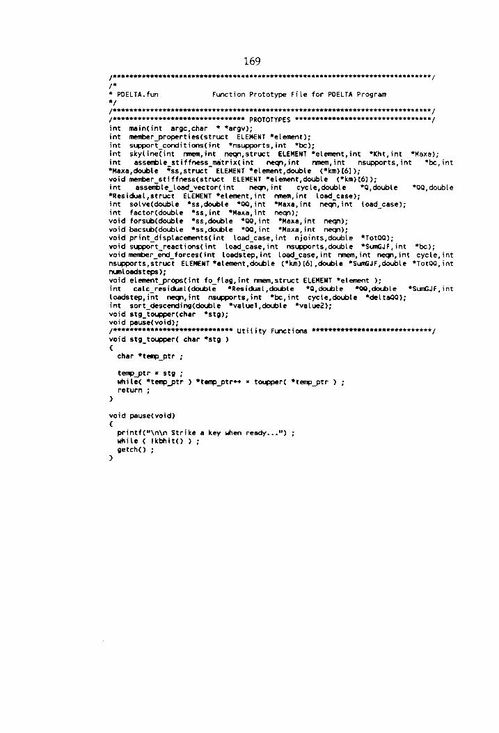
169 [RARE RREAEEEERARRERE NEARER ERERERRERREREEUERERERERREREURREEEREREERENEUREE HE KKK /
/*
* POELTA. fun Function Prototype File for POELTA Program
*/ [AARARARERERRRERERREREARERERHEREREEEREREREEEERERRRERERRRRERERERERERHEERHRHER EK /
[ARRAREARRERARAREERETRERERERHEEER PROTOTYPES PRRAERERREREERENERHEREMEREREKEEE EH f
int maincint argc,char * *argv); int member _properties(struct ELEMENT *element); int support_conditions(int “nsupports,int *bc); int skyline(int nmmem,int neqn,struct ELEMENT *element,int “Kht,int *Maxa); int assemble stiffness _matrixCint neqn,int nmnmem,int nsupports,int *be,int *Maxa,double *“ss,struct ELEMENT *element,double (*km) (61);
void member _stiffness(struct ELEMENT *element,double (*km)[6]);
int assemble_load_vector(int neqn, int cycle, double *Q, double *0Q, double *Residual,struct ELEMENT *element,int mmem,int load_case); int solve(double “ss,double *QQ,int “*Maxa,int neqn,int load_case); int factor(double *ss,int *Maxa,int nean);
void forsub(double ‘“ss,double ‘*QQ,int “Maxa,int neqn); void bacsub(double “ss,double *0Q,int ‘*Maxa,int neqn); void print_displacements(int load_case,int njoints,double *TotQQ); void support_reactions(int load_case,int nsupports,double *SumGJF,int *bc); void member_end_forces(int loadstep,int load_case,int mmem,int neqn,int cycle,int msupports, struct ELEMENT *element,double (*km)[6],double *SumGJF,double *TotQQ,int numl oads teps ) ; void element_props(int fo_flag,int nmem,struct ELEMENT “element ); int calc_residual(double ‘*Residual,double *Q,double ‘“*QQ,double ‘*SumGJF,int loadstep, int neqn,int nsupports,int “bc,int cycle,double ‘del tada); int sort_descending(double “*valuel,double *valuez); void stg toupper(char “*stg); void pause(void); [AUMAAAAAARARERTERATARRERARRER Uti { i ty Funct ions SRATERARARREA AREA RAR KKH HaH Ee /
void stg toupper( char “stg ) €
char *temp ptr ;
temp_ptr = stg; while¢ *temp_ptr ) *temp_ptr++ = toupper( *temp_ptr ) ; return ;
}
void pause( void) ¢
printfC"\n\n Strike a key when ready...') ; while ( tkbhit() ) ; getch() ;
>

170 [EERE RAREERERERARREREREREEREREREEEREREEEERNREE EERE RERERERERREEEREEREREEHEENE f
/* */ /* POELTA.c */
/* */
/* Program to Perform Second Order Elastic Analysis of Rigid Frame */
/* Frame Structures. Program follows the Matrix Displacement Method */ {* of Structural Analysis. Uses NEWTON-RHAPSON solution technique */ /* in order to solve the nonlinear problem. */ /* */ /* Research Team: */ /* Eric J. Wishart.......... ween cece esecesace .-.Research Assistant */ /* Thomas M. Murray, PhD..... pee nese eanceene Principal Investigator */ /* Of The */
/* Charles Edward Via Department of Civil Engineering */ /* Virginia Polytechnic Institute & State University «/ /* Blacksburg, Va. 24061 */
/* */ /* Input file: NUCOR _.deff ; Geometry & Loads */ /* Output files: ASO .dis : Second Order Displacements */ /* LRFD dis } Second Order Displacements */ /* ASD .tmp 3; Second Order Member Forces */ /* LRFO tmp ; Second Order Member Forces */
* *
[staenettnenettanaeteansesenenesinnsseneesttanentenenesenesssiaessetanssenenes,
/* */ /* Program Notes: */
/* */ /* 1. Written for an IBM PC or Compatible Personal Computer */ /* running PC-DOS 3.3 or equivalent. */ /* 2. Developed using the Microsoft Version 6.0 C Compiler */ /* 3. Dynamic Memory Allocation accesses Expanded/Extended Memory, */ /* if present, to solve large DOF problems. */ {* 4. All REAL computations performed in double precision format. */ /* 5. Tangent Stiffness is used for Structural Response to Loading. “/
/* 6. Secant Stiffness is used for Member Force-Deformation Response. */ * *
| ataenanenenenranenseeseretenes Local INCLUDES steteuneseueessstuaessssennsss,
#include "pdelta.h* /* constants, macros, types */ #include "“pdelta. fun" /* function prototypes */ [TAAAAAAAARAAHAATEARARENE Global Variable Declarations SRARTRAETARANENERARAH Eh /
int numloadsteps, fo_flag, ss_compe ; [TAAAAANARLATHAERREERHARHEEE File Pointer Declarations SENATE AAT AAATEREREERERKEN /
FILE *fp input /* Geometry & Loads File */ FILE *fp asd dis /* ASO Displacements file */ FILE *fp asd tmp /* ASD Spec. Check file */ FILE *fp_(rfd dis /* LRFO Displacements file */ FILE *fp trfd_tmp /* LRFD Spec. Check file */ [RRRRERAERAEERERARARREREREREREREEEERER ENO REE EARER ERE HARRERERREERTRERRRER ERK EH /
/* Program Main */ [EARAARERRAAERERAEREREEARRRERE ER ERERARREERRERRRREAEEREREDREREEEEREREERER ERE KH /
me
Me
we
Ne
te
main€ int arge, char *argv[] ) €
/* Local Variables */ double Fy, km(6](6], *ss, *Q, *0Q, *TotQQ, *deltaQQ, *SumGJF, *Residual ; int i, j, loadstep, cycle, load_case, mem, result, eqn,
process, stop, njoints, mmem, neqn, nsupports, “be, *Kht, *Maxa, status = NO ERROR, Active Load Cases ;
char *p char, *filename ; ELEMENT *element ;
/* Print Header for Program */ puts(" PDELTA - Ver. 1.00") ; puts(" Virginia Polytechnic Institute & State University") ;
puts(" Charles E. Via Department of Civil Engineering") ; puts(" Blacksburg, Va. 24061") ; puts(" Copyright 1990, ALL Rights Reserved") ;

171
printfc"\n") ;
/* Check Argument List */ if ( arge <= 2 ) €
puts(" Usage: PDELTA order filename") ; Status = ERROR ;
}
/* Begin Definition of Problem */ if ( status ) /* <<<<< begin first set of status checks >>>>>> */ {
/* Parse Command Line Arguments */ p_char = argv(1) ; // order stg toupper( p char ) ; // ORDER filename = argv({2} ; // filename stg_toupper( filename ) ; // FILENAME
/* Input File Handle */ status = ((fp_input = fopen(filename,"rb")) == NULL ) ? ERROR : NO_ERROR ; if ( !status ) printf("\n File Xs Not Found! \n", filename ) ;
/* -- Initialize Output Files -- */ status = ((fp_asd dis = fopen( "ASD.dis", “w" )) == NULL ) ? ERROR : NO_ERROR ; status = ((fp_asd tmp = fopen( “ASO.tmp", "wb")) == NULL ) ? ERROR : NO ERROR ;
if ( !fo_flag ) €
status = ((fp_irfd_dis = fopen( "LRFD.dis”, "w" )) == NULL ) ? ERROR : NO ERROR
status = ((fp_Irfd_tmp = fopen( "LRFD.tmp", “wb'')) == NULL ) 7 ERROR : NO ERROR
> if ( !status ) puts(" Unable to Open Disk Solution Files...) ;
if ( status ) €
/* Set Environment for Analysis Type */ if (istremp(p_char, "SECOND" )) €
/* -- Assign StepSize for Basic Incremental Load -- */ printf¢(™ Number of Load Increments [1-5]: ") ;
scanf("X%d", &numloadsteps ) ; fo_flag = FALSE ; Active Load Cases = LC ; // Process ASO & LRFD if ¢( mumloadsteps > NUMLOADSTEPS ) numloadsteps = NUMLOADSTEPS ; if ( mumloadsteps <= 1 ) numloadsteps = 1 ;
}
else // First Order selected or
{ // Default to FIRST ORDER
numloadsteps = 1 ; fo_flag = TRUE ; Active_Load Cases = L_C/2 ; // Process ASO
> )
>} {* «<cce< end first set of status checks >>>>>> */
if ( status ) /* <<<<<< begin second set of status checks >>>>>> */
€
/* -- Read General Structure Data -- */ fscanf( fp_input, “Xd Xd Xd “Lf”, &njoints, &mmem, Eprocess, &Fy ) ;
/* -- Degrees of Freedom for Structure (GLOBAL) -- */ neqn = njoints * 3;
/* -- Dynamic Allocation for Structural Model -- */ element (ELEMENT *) calloc( nmmem, sizeof(ELEMENT) ) ; be (int *) calloc( njoints, sizeofCint) >:

172
Q = {double *) calloc( neqn, sizeof(double) ) ; QQ = (double *) calloc( neqn, sizeof(double) ) ;
TotaQQ = (double *) calloc( neqn, sizeof(double) ) ; deltsQQ = (double *) calloc( nean, sizeof(double) ) ; SumGJF = {double *) calloc( neqn, sizeof(double) ) ;
Residual = (double *} calloc( neqn, sizeof(double) ) ; Kht = (int *) calloc( negn, sizeof (int) >; Maxa = (int *) calloc( (neqn+1), sizeof(int) 3
/* -- Check Dynamic Memory Allocations -- */ if ( element == NULL IT be == NULL ) {
puts(" GEOMETRY allocation failed...") ; Status = ERROR ;
> if ( Q@ == NULL [f O@ == NULL [{f TotOQ == NULL [1] deltaQQ == NULL )
{ puts(" LOAD/DEFORMATION allocation failed...") ; status = ERROR ;
) if ( SumGJF == NULL If Residual == NULL ) €
puts(" EQUILIBRIUM allocation failed...") ; Status = ERROR ;
> if ¢ Kht == NULL If Maxa == NULL ) €
puts(" SKYLINE allocation failed...") ; status = ERROR ;
> } /* <<<<<< end second set of status checks >>>>>> */
if ( status ) /* <<<<<< begin third set of status checks >>>>>> */ €
/* -- Set Up Models for Specification Check Post-Processors -- */ fprintf( fp_asd_ tmp, "Xd X.21f Xd", mmem, Fy, fo flag ) ; if ( !fo_flag >) fprintf( fp_Irfd_tmp, "Xd Xd X.2lf", mmem, process, Fy ) ;
/* -- Read Element Geometry Data -- */ printf("\n Reading Structure Geometry...") ;
for ¢ mem = 0 > mem < nmem ; memt+ ) Status = member_properties( &element [mem] ) ;
/* -- Read Boundary Conditions -- */
printf("\r Reading Boundary Conditions...') Status = support_conditions( &nmsupports, be ) ;
me
/* -- Calculate Skyline -- */ printf("\r Determining Skyline Profile...") ; status = skyline( nmem, neqn, element, Kht, Maxa > ;
/* -- Pointer to Structure Stiffness Matrix -- */
if ( (ss = (double *) calloc(Maxa[neqn], sizeof(double))) == NULL )
€ puts(" STIFFNESS allocation failed...") ; Status = ERROR ;
> } /*® «<<<<<< end third set of status checks >>>>>> */
if ( status ) /* <<<<<< begin fourth set of status checks >>>>>> */
< /* Report Analysis Progress */ if ( fo_flag ) printf("\r Performing First-Order Elastic Analysis...\n\n" ) ;
else printfc"\r Performing Second-Order Elastic Analysis...\n\n" ) ;
/* --- Assemble ONCE: First Order Analysis --- */

we
173
if ¢ fo_flag ) /* fo_flag == TRUE */ €
>
ss_comps = FALSE ; result = assemble _stiffness_matrix( neqn, mmem, nsupports,
be, Maxa, ss, element, km) ;
else /* fo_flag == FALSE */ SS_comps = TRUE ;
/* Begin Analysis for All Load Cases */
for ( load_case = 1 ; load_case <= Active Load Cases ; load_case++ ) €
/* -- Write Progress to Output Device -- */ printf ("\r Solving Load Combination # Xd", load case) ;
/* -- Initialize Member Parameters -- */
if ( load_case == 1 ) element_props( fo_flag, mmem, element ) ;
/* -- Initialize Load Case Parameters -- */
memset( Tot0Q, 0, neqn*sizeof(double) ) ;
/* -- Read Loads for this Load Case -- */ for ( i = 0; i < neqn; i++ ) fscanf( fp_input, “*lf", &QCi] ) ;
/* -- Perform the Requested Structural Analysis -- */ for ( loadstep = 1; loadstep <= numloadsteps ; loadstept+ ) {
for ( cycle = 1 ; cycle <= MAXCYCLE ; cycle++ ) €
/* --> Assemble EACH: Second Order Analysis --- */ if ( !fo_flag && ss_comps )
result = assemble stiffness _matrix( negqn, mmem, nsupports, be, Maxa, ss, element, km);
/* -- Assemble the Load Vector -- */ result = assembie_load_vector( neqn, cycle, 2, QQ, Residual,
element, mmem, load case ) ;
/* -- Solve the System of Equations -- */ result = solve( ss, QQ, Maxa, neqn, load case ) ;
if ¢ result == NO_ERROR ) €
/* -- Update Displacement Vector -- */ for ¢ i = 0; i < negn; i++ ) TotQQfi] += QQLi] ;
/* -- Calculate Internal Member Reactions -- */ member _end_forces( loadstep, load_case, nmem, neqn, cycle,
nsupports, element, km, SumGJF, TotQQ, numloadsteps )
/* -- Check if Equilibrium is Satified -- */ stop = calc_residual( Residual, 9, 90, SumGJF, loadstep, neqn,
nsupports, be, cycle, deltaaqQ) ; if ( stop ) €
cycle = MAXCYCLE ;
if ¢ ( loadstep == nmumloadsteps ) ) member_end_forces( loadstep, load_case, mmem, neqn, cycle,
nsupports, element, km, SumGJF, TotQQ, numloadsteps
} else
€ /* -- Print Error Message -- */

174
printf("\r Error Encountered...{SS] NOT POSITIVE DEFINITE:") ; Status = ERROR ;
>
} /* <<<<<< end loop on cycle >>>>>> */
} /* <<<<<< end loop on Loadstep >>>>>> */
/* -- Print Displacements and Reactions -- */ print_displacements( load_case, njoints, TotQaQ ) ; support_reactions( load_case, nsupports, SumGJF, be ) ;
> /* <<<<<< end loop on load case >»>>>> */
/* -- Clean - Up -- */ fcloseall() ; /* Close Input & Output Files */ forget ( element ) ; /* Structural Model Pointer */ forget ( Kht ); /* Column Height Vector */
forget ( Maxa ); /* Main Diagonal Vector */
forget (Q); /* Load Vector */ forget ¢ QQ); /* Incremental Displacements */ forget ( TotQQ ) ; /* Total Displacment Vector */ forget ( deltaQaQ ) ; /* Total Incremental Displacments */ forget ( Residual ) ; /* Residual Force Vector */
forget ( SumGJF ) ; /* Global Joint Force Vector */ forget ( ss); /* Structure Stiffness Vector */
> /* <<<<<< end fourth set of status checks »>>>>> */
/* Terminate PDOELTA */
if ¢ tstatus ) pause() ;
return ( ((status) 7? NO_ERROR : ERROR) ) ;
[ARARAAARARREARRRAREREERERRAERARRRARERERERERRRARREREERBERREERERERREREERERRERERE /
/* Function member_properties */ [RAAARAARAERERAARARERARRAERRRERERENRRRARRERRAERRA ERR RENRNERRARERERERA AREER /
int member_properties( ELEMENT *element ) { double theta ;
/* -- Read: BF, TF, HC, TW, Da, Db -- */ fscanf( fp_input, "Alf Xif Alf ALF RLF RIF ", Selement->BF, &element->TF,
&element->HC, &element->Tw, &element->0a, &element->0b ) ;
/* -- Read: LENGTH, theta -- */ fscanf( fp_input, "If Zi f", Selement->LENGTH, &theta ) ;
/* -- Read: MCODE -- */
fscanf( fp_input; "2d Xd Xd Xd Md Xd", &element->MCOOE (0), &element->MCODE [1], &element->MCODE [2], &element->MCODE (3), &element ->MCODE [4], &element->MCODE [5]) ;
/* -- Calculate and Store Required Section Properties -- */ element->Ag = 2.0*( element ->8F)*(element->TF)+(element->HC)*(element->TW) ;
element->Ix = Celement->B8F)*pow( (element->TF),3.0)/6.0 + , 0.5* (element ->BF)* (element ->TF)*pow( ( (element ->HC)+(element->TF)),2.0)
(element ->TW)*pow( (element ->HC),3.0)/12.0 ; element->SW = (element->Ag)*(element->LENGTH)*DENSITY ; element->COST = cos(theta) ; element->SINT = sin(theta) ;
/* -- Initialize Axial Force -- */ element->P = 0.0;
/* Return to Main() */
return ( NO_ERROR ) ;

175
[AERRARERRRERERAERERRERERRRRERRERERRREERERERERREEEHEREERERERREE EEE EERE RARER EEK 7
/* Function support_conditions */ [ARRRAERRRAKRREEERERRRERRERERHERRRREREREREEREE HERE EERERREREEREREE ERAN ER EERE /
/* msupports -> Number of Boundary Conditions */
/* be(nsup] -> Number of Restrained GOOF */ [RARERREAEKERERERERERRRRRERRRHEREREERERERHAEERENER /
int support_conditions¢ int *nsupports, int “be )
€ int nsup ;
/* Number of support conditions */ fscanf( fp_input, "Xd", nsupports ) ;
/* Read the Boundary Conditions */ for ( nsup = 0 ; nsup < *nsupports ; nsup++ )
fscanf( fp_input, "Xd", &bc(nsup] ) ;
/* Return to Maint) */ return( NO_ERROR ) ;
>
[AARRERARRAAERERRERRERRERERERREREERRRERENERAERREREREEEEERRERERERERHREERR EEE /
/* Function skyline */ [PARARAAHAARARARARREREERRARARRERERARER ERATE EREARARER EATER ERERAEKN AENEAN RAE /
int skyline( int mmem, int neqn, ELEMENT *element, int *Kht, int *Maxa ) € /* Local Variables */ register int i, j : int ndof, mem, dof{(6] ;
/* For all members of the structure... */ for ( mem = 0 ; mem < nmem ; memt++ ) {
/* -- Extract Current Element MCODE -- */ for ¢ ndof = 0 ; ndof < 6 ; ndof++ ) dof {ndof] = element [mem] .MCODE(ndof] ;
/* -- Parse MCOOE for OOF Differentials: Active Column Heights -- */
for¢ jf =O; j <6; j++ ) for¢ i =O; i < 63 ite )
Kht [dof(j}] = min(dof(j], max(Kht{dof(j]],dof{j]-dofli] )) ; )
/* -- Map the Main Diagonal Element Locations -- */ Maxa(0) = 0; for ¢ i = 0; i < neqn; i++ ) Maxali+1]) = Maxali) + Khtli] + 1;
/* Return to Main() */ return ( NO_ERROR ) ;
} [APARRARAERARER ARERR RARER ARREEARERRA RARER RARER HRRERRRERREREREREEEREREREERE RE 7
/* Function assemble_stiffness_ matrix */ [ THAAAARAAA AERA AERAAREERERERRARURRRRERARRARAERERARRRRREEHHAE KERNAN /
int assemble stiffness_matrix( int neqn, int mmem, int msupports, int *bc, int *Maxa, double “ss, ELEMENT *element, double (*km) [6] )
{ int i, j, k, m, dof{6) ;
/* Initialize Structure Stiffness Matrix */ memset( ss, 0, Maxa(neqn] *sizeof(double) ) ;:
/* Assemble For All Elements */
for ( m= 0 ; m < nmem ; m+ ) €
/* -- Retrieve Element MCODE for Mapping to ss(]-- */ for ( i = 0; i <6; i++ ) dofli] = element[m) .MCODE[i) ; e

176
/* -- Assemble Element->System Tangent Stiffness Matrix -- */
for ( j =O; j <6; j++ ) for (k=O; k <6; k++ ) €
if ¢ dof(k] > dof{j] ) continue ; i = Maxa(dof(j]]} + dof{j] - dof{k] ; ss{i] += km(j) (k] ;
) }
/* Invoke Boundary Conditions by PENALTY Method */ for ¢ i = 0 ; i < nsupports ; i++ ) ss(Maxa(be(i}]]] += 1.0e50 ;
/* Return to Main() */ return( NO_ ERROR ) ;
> [EMR ARARURARRRAERRRRURERRERARAERENERERERERRREREARERERRERREREHRERERERERE EERE /
/* Function member stiffness [TANGENT STIFFNESS] */ [PRRRRARRERRARAAAAR AAA RERAERARAERERREARERERRER ERE ER ERED EEE RAA EERE RENEE EER ERNE /
void member_stiffness( ELEMENT *element, double (*km)[6] )
€ /* Local Variables */ double L, alpha, beta, cost, sint, GD(6], GF(6], LF{6],
gi, g2, 93, 94, 95, 96, 97, phi, phic, phit, cl, c2, c3, cos 2t, sin_2t ;
int i, j, axial_ind ;
/* -- Common Factors for Stiffness Coefficients -- */
L = element->LENGTH ; alpha = E*(element->1x)/L/L/L ;
beta = (element->Ag)*L*L/Celement->Ix) ;
/* -- Factor Rotational Stiffness for P-Delta Analysis -- */ if ( fabs(element->P) <= ZERO_STIFFNESS ) axial_ind = 0 ; else if ¢ element->P > 0.0 ) axial_ind = 1 ; else axial_ind = 2 ; switch ¢ axial_ind ) €
case 0: /* No Axial Force, First Order */ €
c1 = 4.0; c2 = 2.0 ; c3 = 6.0;
> break ;
case 1: /* Axial Compression, Second-Order */
€ phi = L*sqrt(Celement->P/(E*element->Ix)) ; phic = 2.0*(1.0-cos(phi))-phi*sin(phi) ; ci = phi*(sin(phi)-phitcos(phi))/phic § ; c2 = phi*(phi-sin(phi))/phic ; cS =cl+c2 :
} break ;
case 2: /* Axial Tension, Second-Order */ €
phi = L*sqrt(-element->P/(E*element->Ix)) phit = 2.0*(1.0-cosh(phi))+phi*sinh(phi) cl = phi*(phi*cosh(phi)-sinh(phi))/phit c2 = _ phi*(sinh(phi)-phi)/phit cS = ci + c2
Bee
Me
Me
Me
we
)
/* Element Direction Cosines */ cost = element->COST ; sint = element->SINT ; cos_2t = cost*cost ;

177
sin_2t = sint*sint ;
/* Tangent Stiffness Elements Computations */
/* -- References */ {* -- Holzer... ccc cee wee w ecw cceeees p. 126 */ [™ => OFAN. cee cece cence cee verennes p. 973 */ gl = alpha * ( beta*cos 2t + 2.0*sin_2t*c3 ) ; g2 = alpha * cost*sint * ( beta - 2.0*c3 ) ; g3 = alpha * ( beta*sin_2t + 2.0*%cos 2t*c3 ) ; g4 = -alpha * c3*L*sint : g5 = alpha * c3*L*cost ; g6 = alpha * c1*L*i : g7 = alpha * c2*L*L :
/* - Upper Triangular Elements - */ /* -- Row. -- */ km(0](0] = gi; km(GJ(1] = g2 ; km(Ol(2] = 94; km(0] [3] = -gl ; km(O} (4) = -g2 ; km(O](5] = 94 ; {*™ -- Row 2 -- */
km{1} 1} = g3 ; km{4) (2) = g5 ; km{[1) [3] = -g2 ; km(i} [4] = -g3 ; km(1](5} = g5 ; /* -- Row 3 -- */ km(27[2) = 96 ; km(2](3] = -g4 ; km(2)(4] = -g5 ; km(2)(5] = g7 ; /* -- Row 4 -- */ km(3J(3] = 91 ; km(31(4] = g2 ; km(3][5] = -94 ; /* -- Row 5 -- */ km(41 (4) = g3 ; km(4)(5] = -95 /* -- Row 6 -- */ km(51(5] = 96;
me
/* Exploit Symmetry of [km] */ for (i =0; i <5 3 it* )
for ( j = Ci*1) 7 j <6 FG j++ ) kmCjI Ci) = kmlil Cj] ;
/* Return to Assemble Stiffness Matrix() */ return ;
) [RAARRRARENARAARARRREEREARRENRREREAERERRDEERERRARRERREREERERRREREERRERERREHEEH /
/* Function assemble load vector */ [BEAARARRAEARAARRARERERERRERAARERRREREURERERRRERRAER ARERR ERERRERREREREREREKEKHE f
/* QQ{row] -> Value of Load at GDOF {row} */ /* or, when cycle != 1 the Residual load */ /* Q- F is reapplied to the structure. */ / ARARARAERARERRERERERRETERRERARRARERAR TROON EEE TEE /
int assemble_load_vector( int neqn, int cycle, double *@, double *QdQ, double *Residual, ELEMENT *element, int nmem, int load.case )
€ int row, mem ;
if ¢( cycle == 1 ) €
double inc, load_fact, node_fact ;
/* Calculate Incremental Load Vector */
ine = 1.0/((double)numloadsteps) ;
/* -- Externally Applied Load -- */ for ¢ row = 0 ; row < neqn ; row++ ) QQ[row] = inc*Q[row] ;
/* -- Selfweight Nodal Loads -- */ switch ( load_case ) €
case 1: case 2: C
load_fact = -1.0 ;

178
} break ; case 3
case 4
case 5
case 6:
case 7
case 8
case 9
case 1
case 11:
case 12:
case 13: case 14:
case 15: case 16:
load_fact = -0.75 ; ) break ; default: {
load_fact = -1.2 ; d
) node_fact = 0.5*inc*load_fact ;
for ( mem = 0 >; mem < mmem >; ment+ ) {
QQ [element [mem] .MCODE(1]] += node_fact*element [mem] .SW ; QQ (element (mem) .MCODE [4]] += node_fact*element [mem] .SW ;
} )
else
€ /* -+ Residual Load Vector -- */ for ( row = 0 ; row < neqn ; rowt+ ) QQ[row] = Residual {row] ;
>
/* Return to Main() */
return ( NO_ERROR ) ;
LRAAAAARAREARARAAAERAURAARARER REET ERATE EEEREREEEAEERERERERHRENEE REET RHEE /
/* Function solve af [RREAREREAREAAARARERRERERERER ERR AE TERA ERA RRENRERREEHEHAERHHEREEKE KKK /
int solve( double *ss, double *QQ, int *Maxa, int neqn, int load case )
¢ /* Local Variables */ int status ;
if ¢ fo_flag ) // FOEA
{ if ¢ load case z= 1 )
Status = ( factor(ss, Maxa, neqn ) == NOTPOSITIVEDEF ) ? NOTPOSITIVEDEF : NO_ERROR ;
else /* 1 < load_case < Active Load Cases */ status = NO_ ERROR ;
} else // SOEA
status = ( factor(ss, Maxa, nmeqn ) == NOTPOSITIVEDEF ) ? WOTPOSITIVEDEF : NO_ERROR ;
if ( status == NO_ERROR )
€ forsub(ss, QQ, Maxa, neqn)
bacsub(ss, QQ, Maxa, neqn) }
we Me

179
/* Return to Main() */ return( status ) ;
[BEAKRAKAHRRERRERERERREEREREREREEEREREREREER ERE EERE REE RRERERER ERE EE EEE KEKE /
/* Function factor */ [EAE RARRRERRRERERREREERREREREREEEERERERERERERRERE HERE RENEE ERE RHEE RERERERER ERE /
int factor( double “ss, int *Maxa, int neqn ) € /* Local Variables */ register int counter1, counter2, counter3; int ic, k, kh, ki, kk, kl, klt, kn, ku, nd; double b, c ;
for ( counterl = 0 ; counter! < neqn ; counteri++ )
{ kn kl ku kh
MaxaCcounter1!) ; kn+1;
Maxa(counter! + 1) - 1; ku > kl;
if (kh < 0)
if ( fabs(ss(kn]) <= ZERO STIFFNESS )
‘ return(NOTPOSITIVEDEF) ; ) }
else if ( tkh )
goto Zero ;
k = counter! - kh ;
ic = 0; klt = ku; for ( counter2 = 0 ; counter2 < kh ; counter2++ ) €
ict++ ; kit-- ; ki = Maxafk) ; nd = Maxa(ik + 1) - ki - 1; if (nd>0)
€ kk = (ic < nd? ic : nd);
c = 0.0; for ( counter3 = 1 ; counter3 <= kk ; counter3++ )
c += ss(ki+counter3] * ( ss(klt+¢counter3) ) ; ss(klt} -=c¢;
> k++ ;
)
Zero:
k = counter! ;
b= 0.0; for ¢ kk = kl ; kk <* ku > kke+ ) {
i = Maxa(k] ; ss(kk] / ss{ki] ;
=c * ss{kk) ; kk] =c;
TO KK
+ ss[
} ss{kn] -=b;
>
/* Return to solve() */

180
return( NO_ERROR ) ; }
[ERRRRERRREREAREERRERERRRERERERERREREERER AREER EREERERREMRER EAH EEE NER EERE MEER /
/* Function forsub */ [ AAARARRARERERARRAREERRAERERRRERREREEEEERAEAEEREREEHRREEREUR EERE RERREERERRKE KE /
void forsub(double *ss, double *0Q, int *Maxa, int neqn) € /* Local Variables */ double c ; int count, kl, ku, kh, kk, k, i;
for ¢ count = 0 ; count < neqn ; count++ )
{ kl = Maxafcount] + 1 ; ku = Maxafcount + 1] - 1; kh = ku- kl; if ( kh >= 0 ) {
k = count ; c= 0.0; for ¢( kk = kl os kk <= ku; kke+ ) ¢
k--3 c +3 ss(kk] * QQ{k] ;
) QQ{count] -=c;
> >
/* Return to solve() */ return ;
LRARRRRERER RATA ERARERAREARAREAEEDEERRERERAHRERRRERERREERRERERREREREREEHEENR EHH /
/* Function bacsub */ [MEARE RA AERA AAA RARER RERAEAAEEE AREER RRARERERERRAREHREREEREERREREEEREEER EEK 7
void bacsub( double "ss, double *QQ, int *Maxa, int neqn ) € /* Local Variables */ int count!, count2, k, kl, ku, kk, kh, i ;
for € count! = 0 ; count! < neqn ; counti++ ) €
k = Maxa[count?) ; QQ{count1] /= ss(k] ;
>
if ¢( neqn == 1) return ;
count! = neqn:- 1;
for ¢ count2 = 1 ; count2 < neqn ; count2++ ) €
kl = Maxa[count!] + 1; ku = Maxa[countl + 1} - 1 kh = ku - kl ; if ¢ kh ># 0 ) €
k = counti ; for ¢ kk = kl ; kk <= ku ; kk++ )
{ k-- 5 QQ{k} -= ss{kk}) * QQ[count1) ;
> > counti-- ;

181
/* Return to solve */ return ;
} [ARRRRRE RRR ARR ER ERRRERERERAEREREREEREREEREEEERREEERRERRURERRERERERRE NEHER EK /
/* Function print_displacements */ [RAAERARARAERRERAAREERAREREERERAERERREEEREEEEREERERREREEEEREREEREEURA HERRERA EH /
void print_displacements( int load_case, int njoints, double *TotaQQ )
€ /* Local Variables */ int jt, dof ;
/* -- Adjust "Zero" Displacements -- */ for ( dof = 0; dof < 3*njoints ; dof++ ) €
if ( fabs(TotQ@{[dof]) < 1.0e-6 ) TotQQ{(dof) = 0.0 ;
>
/* Print to Appropriate File */ if ( load_case <= 16 ) €
fprintf( fp_asd_ dis, "\n ASO Load Case No. %d\n", load case ) ; fprintf( fp_asd dis, "\n Jt Global Displacements") ; fprintf( fp_asd_dis, "\n # Xin] Yin) Zirad]") ;
for ¢ jt = 0 > jt < njoints ; jt++ )
fprintf( fp_asd dis, "\n %Ad", jt+l ) ; for ( dof = 0 ; dof <3; dof++ )
fprintf( fp_asd_dis, "% 10.61f", *(TotQQ+dof+3*jt) ) ; >
fprintf( fp_asd dis, "\n" ) ;
) else €
fprintf( fp_lrfd_dis, “\n LRFO Load Case No. Xd\n", (load_case-16) ) ; fprintf( fp_irfd_dis, “\n Jt Global Displacements") ; fprintf( fp_Irfd_dis, "\n # XCin) YCin) Z{rad}]") ;
for ( jt 20; jt < njoints ; jr++ ) €
fprintf( fp_irfd_dis, "\n 4d", jt+l > ; for ( dof = 0; dof <3; dofe+ )
fprintf( fo_lrfd_dis, "% 10.6Lf", *(TotQQ+dof+3*jt) ) ; >
fprintf( fp_(rfd_dis, "\n" ) ; d
/* Return to Main(€) */
return ;
[MPRREREE AREER RARER ARRAREE RARE ERA EREEREREERERRRERERARERRRERRRREREERRRRERREE RED /
/* Function support_reactions * 7 [REAR AREE EEE RREAAER ARERR REREREERRREEERAEEREREKEERERRURRREREREERRRE HER EK H /
void support_reactions( int load case, int nsupports, double *SumGJF, int *be ) { int row ;
/* -- ASD Load Cases -- */ if ( load_case <z 16 ) €
fprintf( fp_asd_dis, "\n OdOF Support Reactions") ; fprintf( fp_asd_dis, “\n #") > for ( row = 0 ; row < nsupports ; row++ )
fprintf( fp_asd_dis, "\n *4d % 10.41", *(be+row)+1, SumGJF [bc {row]] ) ; fprintf¢ fp_asd_dis, "\n\n* ) ;
> /* -- LRFD Load Cases -- */ else €
fprintf( fp_irfd_dis, “\n DOF Support Reactions") ;

182
fprintf( fp_lrfd_dis, "\n #") ; for ( row = 0 5 row < msupports ; row++ )
fprintf( fp_irfd_dis, "\n Xd % 10.41f", *(be+row)+1, SumGJF (be(row]] ) ; fprintf( fp_lrfd_dis, "\n\n" ) ;
}
/* Return to Main() */ return ;
} [RAAARRARARRRAREREEREREERERRERERARRERRERARRURRRRER EERE ARERERRERHURERHERERREE EE /
/* Function member end forces [SECANT STIFFNESS] */ [PRREARARTREREERRERERRERA RRR ERARREREEER AREER EERE REEEEER ERED EERE ER EEEREE RENE /
void member _end_forces( int loadstep, int load_case, int nmem, int neqn, int cycle, int nsupports, ELEMENT *element, double (*km) (61, double *SumGJF, double *Totdaa, int numloadsteps )
{ /* Local Variables */ double L, alpha, beta, cost, sint, GO(6], GF{6], LF{6],
91, 92, 93, 94, 95, 96, 97, phi, phic, phit, phil, phi2, phi3, phi4, load_fact, factor, node_fact, cos _2t, sin_et, half_self_weight, sign ;
int mem, i, j, axial_ind ;
/* -- Initialize Joint Forces -- */ memset( SumGJF, 0, neaqn*sizeof(double) ) ;
/* +> Load Factors for Structure Selfweight -- */ factor = ((double)loadstep)/( (double )numloadsteps) ; switch ( load case ) €
case 1: // ASO Load Cases +0 inc.
case 2:
load_fact = -1.0 ; > break ; case 3: // ASD Load Cases +1/3 inc.
oo
Ge
se
88
case 16:
load_fact = -0.75 ; } break ; default: // LRFD Load Cases {
load_fact = -1.2; d
> node_fact = 0.5*factor*load fact ;
/* -- Loop For ALl Members -- */ for ( mem = 0 ; mem < mmem ; mem+ ) €
/* -- Common Factors for Stiffness Coefficients -- */ L = element [mem) .LENGTH ;

183
alpha = E*(element [mem] .Ix)/L/L/L ; beta = (element [mem] .Ag)*L*L/(element [mem] .Ix) ; half_self_weight = node_fact*element [mem] .SW ;
/* -- Factor Rotational Stiffness for P-Delta Analysis -- */
if ( fabsCelement (mem) .P) <= ZERO STIFFMESS ) axial _ind else if ( element [mem] .P > 0.0 ) axial_ind else axial_ind switch ( axial_ind ) €
case 0: /* No Axial Force, First Order */ €
phil = phi2 = phi3 = phi4 = 1.0; > break ;
case 1: /* Axial Compression, Second-Order */ {
phi = L*sqrt(Celement [mem] .P)/(E*element (mem) .1x)) phic = 2.0*(1.0-cos(phi))-phi*sin(phi) phil = phi*phi*phi*sin(phi)/(12.0*phic) phi2 = phi*phi*(1.0-cos(phi))/(6.0*phic) phi3 = phi*(sin(phi)-phi*cos(phi))/(4.0*phic) phi4 = phi*(phi-sin(phi))/(2.0*phic)
) break ;
case 2: /* Axial Tension, Second-Order */ €
phi = L*sqrt((-element (mem) .P)/(E*%el ement (mem) .1x)> phit = 2.0*(1.0-cosh(phi))+phi*sinh(phi) phil = phi*phi*phi*sinh(phi)/(12.0*phit) phi2 = phi*phi*(cosh(phi)-1.0)/(6.0*phit) phi3 = phi*(phi*cosh(phi)-sinh(phi))/(4.0*%phit) phi4é = phi*(sinh(phi)-phi)/(2.0*phit)
nou
Nu =o
~e
Ma
we
we
fa
Se
we
TE
He
me
wh
Be
Me
BE
Ne
}
/* Element Direction Cosines */ cost = element (mem] .COST ; sint = element (mem] .SINT ; cos _2t = cost*cost ; sin_2t = sint*sint ;
/* Secant Stiffness Elements Computations */ /* -- References */
| hol .(°) © 5 | a p. 126 */ /* -- Chen & Lui... ew eee p. 257 */ gi = alpha * ( beta*cos 2t + 12.0*sin_2t*phil ) ; ge = alpha * cost*sint * ( beta - 12.0*%phil ) ; g3 = alpha * ( beta*sin_2t + 12.0%cos_2t*phil ) ; g&4 = -alpha * 6.0*L*sint*phi2 :
g5 = alpha * 6.0*L*cost*phi2 ; g6 = alpha * 4.0*L*L*phi3 ; 97 = alpha * 2.0*L*L*phié :
/* Upper Triangular Elements */ /* -+ Row 1 -- */ km(O} {0} = gt; km(0)(1]) = g2 ; km[0](2] = g4; km(O} (3) = -g1 ; km(0) (4) = -g2 ; km(0) (5) g4 /* -- Row 2 -- */ kmCVW £1] = g3 3 km€1)(2) = 95 ; km(1] [3] = -g2 ; km{1} (4) 3 -g3 ; km{1)[5]) = g5 ;
km(2}(2] = 96 km(2} {5} = 97 ; {* -- Row 4 -- */ km({3] (3) = g1 ; km{3)[4] = g2 ; km[3](5] = -g4 ; [* -- Row 5S -- */ km(4) (4) = g3 ; km[4)(5) = -g5 ;
s* =» Row 3 -- */ : km(2)(3) = -g4 ; km[2) (4) = -g5 ;

184
/* -- Row 6 -- */ km(5] (5) = 96;
/* Exploit Symmetry of {km) */ for ¢ i =0; 1<S 35 i++ )
for ¢ j = Ci*t1) 5 jf < 6 3 j++ ) kmCj) Cid = kmfiy tj) ;
/* Extract Global Displacements a Active Joints */ for (1 =0; i <6; i++ ) GOCi] = TotQQ[element [mem] .MCODE[I]] ;
/* Calculate Global Member End_Forces */ for ¢ i = 0; i <6; i++ )
GFCi] = 0.0;
for( j = 0; j < & | j++ ) GFLi) += kmCi) (j]*GOCj) ; )
/* -- Global Joint Forces -> ( (f+fp> = [k]{d} ) -- */ for ¢ 1 =0; i <6 3 i++ ) SumGJF( element [mem] .MCODE[i] ] += GFL] ;
/* -- Global Joint Forces -> ( (f} = (k](d) - (fp) ) -- */ /* -<- Selfweight, applied Vertically at End Nodes ->- */ SumGJF [element [mem] .MCODE[1]] -= half_self_weight ; SumGJF element [mem] .MCODE [4}] -= half_self_weight ;
/* Calculate Axial Force for next SOA Cycle: (f} = [k]{(d} - (fp) */ if ( I!ss_comps ) element [mem] .P = 0.0 ; else C
Gouble P1, P2 ; PI cost*GF(0] + sint*(GF[1] -half_self_weight) ; Pe cost*GF(3] + sint*(GF(4]-half_self_weight) ; if ¢ P1>Q) sign= 1.0; else sign = -1.0; element [mem] .P = sign * max( (fabs(P1)) , (fabs(P2)) ) ;
}
/* Save Forces to Files on Completion */ if ( cycle == MAXCYCLE && loadstep == numloadsteps ) €
int index ; FILE *fp_ tmp ;
/* -- Local Forces -> €f)} = [k]{d} - (fp) -- */ LF(O} = cost*GF(0] + sint*(GF[1)-half_self_ weight) ;
LFC1] = -sint*GF(O} + cost*(GF[1]-half_self_weight) ; LF(2] = GF(2] ; LF(3] = cost*GF(3] + sint*(GF(4]-half_self_weight) ; LF([4] = -sint*GF(3] + cost*(GF(4]-half_self_weight) ; LFCS) = GF{(5} ;
/* -- Store -- */ fp_tmp = ( load_case <= 16 ) ? fp_asd_tmp : fp_Irfd_tmp ; for ( index = 0; index <6; index++ ) €
if ( fabs(LF [index] ) < ZERO_STIFFNESS ) LF{index] = 0.0 ; fprintf( fp tmp, “ %.41f", LFLindex) ) ;
}
>
} /* <<<<<< end loop on mem >>>>>> */
/* Return to Maint) */ return ;
)
[AAAARARTRARAARERARRERAERAAREAREH EERE RREREERERRERERERREEHRERUURRUEE REED eakee /

185
/* Function element_props */ [RAR RAE REE ERA RERRERERKEREREERRE REE EEE AEREREH EERE EER AER REE RE EHR EEN HK /
void element_props( int fo_flag, int nmmem, ELEMENT “element ) { double bf, tf, tw, hea, heb, Aga, Agb, Sxa, Sxb, Zxa, Zxb, Ixa, Ixb, ly ; int mem ;
/* -- Calculations of Section Properties for Specification Checking -- */ /* -- Store Properties at A-End & B-End for Proper Interaction Sums -- */ for ¢( mem = 0 ; mem < nmem ; mem++ )
€ bf = element (mem) .BF ; tf = element [mem] .TF ;
tw = element [mem] .TW ; hea = element (mem] .Da - 2.0*tf ; hcb = element [mem] .Db - 2.0*tf ; Aga = 2.0*bf*tf+hca*tw ; Agb = 2.0*bf*tf+hcb*tw ; Ixa = (bf*pow(tf,3.0)/6.0)+(bf*tf*(hcastf)*(hcat+tf)/2.0)+( tw* pow (hca,3.0)/12.0); Ixb = (bf*pow(tf,3.0)/6.0)+(bf*tf*(hcbetf)*(hcbetf)/2.0)+( tw*pow(hceb,3.0)/12.0); Sxa = 2.0*Ixa/element [mem] .Da ; Sxb = 2.0*Ixb/element [mem] .0b ; Ty = tf*pow(bf,3.0)/6.0 ;
/*** -- Store im ASO temporary file -- ***/ fprintf( fp_asd_tmp, " X.41f K.41f X41 Ff", bf, tf, tw) ; fprintf( fp_asd_tmp, “ %.41f Z.3Lf Z.3Lf X.3Lf", hea, Aga, Ixa, Sxa ) ;
fprintf( fp_asd_tmp, " X.41f %.31f X.3If 31 Ff", heb, Agb, Ixb, Sxb ) ; fprintf( fp_asd_tmp, " %.31f", ly ) ;
if ¢ tfo_flag ) /*** -- Store im LRFD temporary file -- ***/ €
Zxa = bf*tf*(hcattf) + hca*hca*tw/4.0 ; zZxb = bf*tf*(hcbetf) + hceb*hcb*tw/4.0 ; fprintf(fp_lrfd_tmp,” %.4lf X.41f Z.4lf", bf, tf, tw); fprintf(fp_lrfd_tmp,” Z.4lf Z.31f RSF SSF Z.31f", hea, Aga, Ixa,Sxa,Z2xa) ; fprintf( fp (rfd_tmp," Z.41f Z.31f Z.31f Z.3UF X31 fF", heb, Agb, Ixb,Sxb,Z2xb) ; fprintf(fp_lrfd_tmp,” *.31f", ly ) ;
>
>} /** next [mem] ber **/
/* -- Return to maint) -- */ return ;
} /*** end of element_props ***/ [RARAAAARSAAERAERAARAAE AREA ERAERARERATERERERARER REAR EERERRRERRERERER AREER /
/* Function cale_residual */ | hakahniatehaiahehaiatalatabehaictahaiahainiabahahatahahaiatehsatehatatahehabataiateheiataihatehaishabehaiaheiahaheiaiateietatateiatehalateletahettaheled |
int calc_residual( double *Residual, double *Q, double *0Q,
double *SumGJF, int loadstep, int neqn, int nsupports, int *be, int cycle, double *delraaa }
€ /* Local Variables */ double factor, num_d, den_d, disp_check, force_check ; int k, flag;
/* Second Order Anatysis - Calculate Convergence Parameters */
if ( ss_comps ) €
/* Initialize Steps - Sum Increment */ if ( cycle == 1 )
memcpy( deltaQ@, QQ, neqn*sizeof(double) ) ; else
for ( k = 0; k < neqn ; kt+ ) deltaQa{k] += QQ(k] ;

186
/* Displacement Convergence Parameters */ qsort¢( QQ , neqn, sizeof(double), sort_descending ) ;
qsort( deltaQQ, neqn, sizeof(double), sort_descending ) ; num_d = fabs¢*QQ) ; // Maximum Increment this Cycle den_d = fabs(*deltaQaQ) ; // Maximum Displacement this Step den_d = max(den_d, CPOB) ; // Trap Division by Zero disp_check = (num_d/den_d/CPDB) ; // Normalized Displacement Check
/* -- Calculate External Load, Form the Residual -- */ factor = ((double)loadstep)/((double)numloadsteps) ; for (kk =0; k < neqn ; k++ ) {
QQ[k) = factor * Q[(k] ; //a Residual {k) = QQ{k] - SumGJF{k] ; 4/Q-F
>
/* Absorb Residuals at Boundaries */ for « k = 0; k < nsupports ; k++ ) Residual [be(k]] = 0.0 ;
/* Force Convergence Parameters */
memcpy( SumGJF, Residual, neqn*sizeof(double) ) ; qsort( SumGJF, neqn, sizeof(double), sort_descending) ; force check = fabs(*SumGJF)/CPFB ; // Normalized Force Check
} else /* First Order Analysis Was Requested */
€ disp check = force check = 1.0 ;
>
/* -- Equilibrium Check -- */ flag = ¢ (disp check <= 1.0) && (force_check <= 1.0) ) ? TRUE : FALSE ;
/* Return to Maint) */
return( flag ) ;
d [LAAARARAAAREREARARRACRERARRERERAERERRERERRARRRRERERREREEREHRERARERERRAREHER ER /
/* Function sort_descending (called by qsort in calc_residual) */ [ARAHAARAAAAAAAERARARARRERRRERRERETEEEHREERAEREERERRRERTANERERREREEHREREHREE /
int sort_descending( double *valuel, double *value2 ) { int result ;
/* Define qsort Ordering Rules */ if ( fabs(*valuel) > fabs(*value2) ) result = -1; // Larger else if ¢( fabs(*valuel) < fabs(*value2) >) result = 1; // Smaller else result = QO; /f Equal
return(result) ; > [ARRAAAARAAARERERARRREARREREREREREEREEREREARERERERERRERERERRERRERERRRER HE /
/* End POELTA Program */ [RARAARTRRARARARAERERERERRRRRREREHERERHRARHERARRERRERRRRRRARARRERARREREHRERRENY /

187
ASDSPEC.c

188 [REMRRRRERARRRRRRER AREER EERE ARERR ER ARR RREEREEEREERE REE AREER EER ERE EERE ERE REE /
/*
* ASDSPEC.h Header File for ASOSPEC Program
*/ [RARER AERENERAREEREREERREREREEEEE CONSTANTS RARER ARERERREREERERENREREREERE /
#define E 29000 .0
#define PI 3.161592653589793
#define TRUE 1
#define FALSE 0 [AAARARRERERRERRERERERERRERERREREE MACROS SAAERARAARRRERAEREREERRRREAHRREREKRE EE /
#define forget(x) { if (x) free((void *)x) ; x = NULL ; } [J REAAAARARA RARER RRRERERRRRRR TEER STRUCTURES RARARRARERRERRERREEEEHAEREREREREKE /
typedef struct ELEMENT €
double 8F, /* Flange Width */ TF, /* Flange Thickness */
TW, /* Web Thickness */ HCA, /* Web Height, A-End */ AGA, /* Area of Element A-End */
IXA, /* X-X Moment of Inertia A-End § */ SXA, /* Elastic Section Modulus A-End */ HCB, /* Web Height, 8-End */ AGB, {* Area of Element 8-End */ 1X8, /* X-X Moment of Inertia 8-End = */ SXB, /* Elastic Section Modulus B-End */ ly; /* Y-Y Moment of Inertia */
> ELEMENT ; [PATRARRERARARRERRRERRERRAREREREER FUNCTIONS RREAHARARARRRRRAERERERERERRERERE NH /
extern int main (void); extern void read_input(int i); extern void code_check(int i); extern double axial _capacity(int i); extern double shear_capacity(void); extern double moment_capacity(int i); extern void combined stress(double Pa,double Va,double Ma, int 1); extern void critical _ratiosCint i,double stability,double capacity,double shear); extern int member _properties(ELEMENT *element); extern void pause(void); J MAAHORAARANAARRRARRERERERRERE Character Strings SARA RTAEAAREARAARARRRAEEAREN ED /
/*
* Load Combination Titles for ASO Analysis\Design */ static char *str(] = ¢ "1.00 * ( D+ SL + SR)",
"1.00 * (0D + SL + SR/2 }" ,
"0.75 * (0 + WLLI1 + WLRI DD" ,
"0.75 * (D+ WLL2 + WLR2 >" ,
"0.75 * ( D + SL + SR + WLLI/2 + WLRI/2 )” ,
"0.75 * (0D + SL + SR + WLL2/2 + WLR2/2 " ,
"0,75 * ( D + SL + SR/2 + WLLI/2 + WLRI/2 )" , "0.75 * (D+ SL + SR/2 + WLL2/2 + WLR2/2 )" ,
"0.75 * ( D + SL + SR/2 + WRL1/2 + WRRI/2 )" , "0.75 * ( D + SL + SR/2 + WRL2/2 + WRR2/2 )" ,
"0.75 * ( D + SL/2 + SR/2 + WLL1 + WLRI )" ,
"0.75 * ¢ 0 + SL/2 + SR/2 + WLL2 + WLR2 >* ,
"0.75 * (0 + SL/2 + SR/4 + WLL1 + WLRT )" ,
"0.75 * ( D + SL/2 + SR/& + WLL2 + WLR2 )" ,
“0.75 * ( D + SL/2 + SR/4 + WRL1 + WRRI D>" ,
"0.75 * ( 0 + SL/2 + SR/4 + WRL2 + WRR2 )" );

189 [AREER ERERARARERERERRREE RAE RRERRERENENRRENEHENEREREREREREREUEEKKEERKKE HERE MERE /
/* */ /* ASDSPEC.c */
/* */ /* Copyright 1990, PC Structural Engineers */
/* Blacksburg, Virginia 24060 */ /* */ /* Research Team: */ /™ Eric J. Wishart... . ccc cece ccc wceccceeee Research Investigator */ /* Thomas M. Murray, PhD....... eseene eeeees Principal Investigator */ /* Of The */
/* Charies E. Via, Jr. Department of Civil Engineering */ /* Virginia Polytechnic Institute & State University */
/* Blacksburg, Virginia 24061 */
/* */ /* Sponsor: NUCOR Metal Building Products «/ /* Waterloo, Indiana */ /* */ /* Performs Code Checking of Beams, Columns, and */
/* Beam-Columns according to the AISC 9th Edition ASO Specification. */
/* Second Order Analysis Results NOT REQUIRED. */ /* */ /* Only error recognized at this point, is the calculation of Cb. By */ /* definition, it is calculated using the moments at the ends of the */ /* umbraced length (unless larger in-between). This program assumes */
/* the “end” moments are located at each discretized element “end". */
/* The error in the calculation will be a conservative one. */ /* */ /* InputFile: ASO. tmp */ /* OQutputFile: ASO .chk */
/* */ [SAAAREERERRARREREERE RARER RERERREEEERERERERERAERRERERERE HERRERA ERERER HR ERE RAE HE /
/* INCLUDE files */
#include <stdio.h> /* Microsoft Library */
#include <math.h> #include <fcntl .h>
#include <stdlib.h>
#inctude <conio.h> #include <malloc.h>
#include <conio.h> #include "ASOSPEC.h® /* ASDSPEC header file */
/* DEFINE constants */
#define ERROR 0
Bdefine NO_ERROR 1
/* Global Variables */ double P,V,M,M1,M2,Sx,bf,tf,hc,tw,Ix,ly,Ag,
KLx [200] ,KLy (200) ,Fy,Fa,Fv,Fo,rx,ry,KL_rx,KL_ry,KLmax,FS,
kc, lambda_FL8, lambda WLB,(p FLB,lr_FLB,lp_WLB,lr_WLB, Sx, Ix, AQ, “SR, *CR, "VR, Q, FORCE[6] ;
int nmem,i,load_case, fo_flag, *Stab_Case, *Cap Case, *Shear Case ; ELEMENT *element ; FILE *in, *in2, *out, *max_ratios ;
/* Main Program */
main() € int status = NO_ERROR ;
/* Open Output File for Writing */ out = fopen("ASO.chk", “wit) ; max_catios = fopen("ASO.sum","wit) ; if ¢ out == NULL If max_ratios == NULL ) €
printf("\n CANNOT OPEN FILES ASD.chk or ASO.sum'') ;
status = ERROR ;
pause() ;

190
>
/* Open Input Files for Reading */
in = fopen("ASD.tmp","rb") ; ind = fopen("KL.fct","r") ;
if ¢€ im == NULL f2 im2 == NULL )
€ printf("\n CANNOT OPEN FILES, ASO.tmp or KL.tmp") ;
status = ERROR ;
pause() ; >
if ( status )
€ /* Report and Progress With Solution */ printf("\n ASO 9th Edition Specification Check In Progress...\n\n") ; fscanf(in, "Xd XLf Xd", &rmem, &Fy, &fo_flag );
/* Dynamic Memory Allocation */ element = (ELEMENT *) calloc( mmem, sizeof(ELEMENT) ) ; SR = (double *) calloc¢ mmem, sizeof(double) ) ;
CR = (double *) calloc( nmmem, sizeof(double) ) ; VR =z {double *> calloc( nmmem, sizeof(double) ) ; Stab Case = (int *) caltoc( nmem, sizeof(int) ) ; Cap Case = (int *) calloc( nmem, sizeof(int) ); Shear Case = (int *) calloc( nmem, sizeof(int) );
/* -- Check Dynamic Memory Allocations -- */ if ¢ (element == (ELEMENT *) NULL) )
status = ERROR ;
if ( (SR == NULL) IT (CR == NULL) IT (VR == NULL) ) status = ERROR ;
if ( ¢Stab_Case == NULL) If (Cap_Case == NULL) ff cvR == NULL) )
Status = ERROR ; if ( !status )
€ fcloseall() ; return(€ ERROR ) ;
>
/* Read in Member Properties & Bracing Factors */ for ( i = 0; i < nmem; i++ ) €
status = member_properties( &element(i] ) ; fscanf(ind, "%lf Lf", &KLx{[i], &KLyli] ) ;
) fclose( ing ) ;
/* Process All Load Combinations */ for ( load_case = 0 ; load case < 16 ; load_caset+ ) {
/* -- Report Progress -- */ printf("\r ASO Load Combination No. %d", load_case+1 ) ;
/* -- Title to OutputFile -- */ fprintf(out, “\n ASO Load Combination No. %d", load case+! ) ;
fprintf(out, “\n = z= ze\n\n" ) ; fprintfCout,"\t%s\n", str(load_ case] ) ; fprintfCout, "\n Mem P v M Pa Va Ma
Stability Capacity” ); fprintfCout, "\n # (k] (k) (kft) {k} {k) {kft)
(Unityl] (Unity]" ); fprintfCout, M\N mere creer cert rere t ere rete e er creer secre
/* -- Process All Members -- */
for ¢ i = 0; i < mem; i++ ) €

191
read_input(i) ;
/** -- Process a-end -- *¥*/ fprintf(out, ""\n %3da",i+1) ; he = element(i].HCA ; Ag = element[i].AGA ; Sx = element[i] .SXA ; Ix = element[i] .IXA ; P = FORCE(O] ; V = FORCE[1] ;
M = FORCE(2) ;
code_check(i) ;
/** -- Process b-end -- **/ fprintfcout,"\n %3db",1+1) ; he = element(i].#CB ; Ag = element[i].AGB ; Sx = element(i].SxB ;
Ix = element[i].1xB ; P = -FORCE[3] ;
V = FORCE[4] ;
M = FORCE(5] ; code_check(i) ;
> fprintfcout, "\n" >) ;
)
/* -- Save Summary File -- */
// Check A-End
// Check B-End
fprintf(max_ratios,"\n\t Summary of 9th Edition ASD Specification Checking\n") ; fprintf(max_ratios,"\n\t Table of Maximum Design Ratio Locations\n") ; fprintf(max_ratios,"\n\t Member Stability Stability Capacity Capacity Shear
Shear") ;
fprintf(max_ratios,"\n\t = No. Case# Ratio") ;
fprintf(max_ratios,"\M\t ------ correo: eeeee ") >;
for ( i = 0; i < mmem; i++ )
Ratio Case# Ratio Case#
ee ee ae
fprintf(max_ratios,"“\n\t 6d 29d Z9.41f XBd MB.41f XSd X5.41f", (i+1), (Stab Case[ij+1),
/* -- Close ifo Fites -- */
fcloseall() ;
> /*** end status check ***/
/* Completed */ printf¢("\n") ;
return( status ) >
> /*** end maint) ***/
void read_input(int i) € int index ;
/* -- Read Member Reactions -- */ for ¢ index = 0; index < 6 >; index++ )
fscanf(in, “%Lf", &FORCELindex) ) >
/* -+ Assign Element Properties -- */ bf = element(i].BF ; tf = element{i].TF >; tw ly = element{i].1Y >
/* -- Rotational Moments for Cbd Computation Mi =
M2 =
/*® Return to Main() */
SR(i],(Cap Caseli]+1), CRLi]),(Shear_Case(i]+1),VR{i) > ;
= element[i).TW ;
=< wy
( fabs(FORCE(2]) <= fabs(FORCE(5]) ) ? FORCE [2) ( fabs(FORCE(2}]) >= fabs(FORCE(S]) ) ? FORCE [2)
: FORCE(S? ;
: FORCE(S] ;

192 return ;
> /*** end read_input ***/
/* Code Check Subprogram */ void code_check(int i) { double Pa, Va, Ma;
Pa
Va
Ma
axial _capacity¢i) ; shear_capacity() ; moment _capacityci) ;
fprintfCout, " X+#7.21f Xe7.21f Xe. .21 Ff XAe7.2LF A7.2F AO.21 Ff", P, V, M/12.0, Pa, Va, Ma/t2.0 ) ;
combined _stress(Pa,Va,Ma,i) ;
/* Return to Maint) */ return ;
)
double axial _capacitycint i) € double Pa, Qs, Qa, f, f_new, beff, C_c, Ca, inc ; int convergence ;
/* Initialize Parameters */ rx = sqrtcIx/Ag) ; ry = sqrt(ly/Ag) ; KL_cx = KLxCil/ex ; // In-Plane Slenderness KL_ry = KLylil/ry ; // Qut-Of-Plane Slenderness Kimax = max( Kiorx, KlLiry ) ; // Maximum Slenderness Ratio Pa = 0.0; // Allowable Axial Load a2=1.0; // Section Efficiency convergence = FALSE ; // Used with Slender Sections inc = ( load_case <= 1) 71.0 : 0.75 ; // 1/3 Stress Increase
/* Local Buckling Parameters */
Lambda _FLB = bf/(2.0*tf) ; // Flange Slenderness
lambda_WLB = hc/tw ; // Web Slenderness
/* -+- 9th Edition Update -- */ /** Reflects Research by Butler Manufacturing Co. **/ /** on Local Flange/Web Buckling interaction. "kc" **/
/** is a plate buckling coefficient for h/t > 70 ‘**/ ke = ( (he/tw) > 70.0 ) ? 4.05/pow( lambda _WLB, 0.46) : 1.0 ;
/* Tension or Compression? */ /** Analysis Passes Axial forces as +C and -T **/
if ¢ P <= 0.0 ) €
/* Allowable Tensile Stress: Gross Section */ Fa = -0.60*Fy ; Pa = Ag*Fa ;
)} /*** end tensile allowable force ***/
else €
/* Compression Capacity */ C_c = sqrt(2.0*PI*PI*E/Fy) ;
/* Local Buckling Limits, Table 85.1 */
lr_FLB = 95.0/sqrt(Fy/ke) ; // Flange Noncompact Limit ir_WLB = 253.0/sqrt(Fy) ; // Web Noncompact Limit

193
if ( lambda _FLB <= Ur_FLB && lambda WLB <= tr_WLB ) /* Section Composed of (Non)Compact Element(s) */ /** Chapter E **/ {
if ¢ KLmax <= Cc )
Ca = KLmax/C_c ; FS = 5.0/3.0 + 0.375*Ca - 0.125*Ca*Ca*Ca ; /* Allowable Compressive Stress: Compact, Inelastic */ Fa = ( 1.0 - 0.5*Ca*Ca )*Fy / FS ; Pa = Ag*Fa ;
} else if ¢ KLmax > Cc ) {
FS = 23.0/12.0 ;
Fa = PI*PI*E/(KLmax*Kimax) / FS ; Pa = Ag*Fa ;
} }
/* Allowable Compressive Stress: Compact, Elastic */
else /* Section Composed of Slender Element(s) */ /** Section Composed of Slender Element(s) **/ {
if ¢ lambda_FLB > Ir_FLB ) // Unstiffened Elements
/* Flanges Slender */ if ¢ lambda FLB < (195.0/sqrt(Fy/kc)) )
Qs = 1.293 - 0.00309*lambda FLB*sqrt(Fy/ke) ; else
Qs = 26200.0*kc/(Fy*lambda_FLB* lambda FLB) ; ) else €
Qs = 1.0 ; > Qs = min ( Qs, 1.0 ) ; // Error Check
ITERATE:
if (lambda _WLB > (r_WLB) // Stiffened Elements €
/* Web Slender */ Pa = ( Pa ) 7? Pa: 0.60*Fy*Ag ; f = sqrtCince*Pa/Ag) ; if ( f ) // Effective Width of Web? ¢
beff = (253.0*tw/f)*(1.0-44.3/( lambda WLB*f)) ; if ( beff >= he ) beff = he ; if ¢ (beff/tw) < l[r_WLB ) beff = min( (ir_WLB*tw), he ) ; Qa = (Ag-C(he-beff)*tw)/Ag ;
> else // Reduction Insignificant
{ Qa = 1.0;
> > else // (Non) compact €
Qa = 1.0;
>
/* -- Q@ = Efficiency Factor, or Reduced Section Factor -- */ /** -- Theoretically, the ratio of Fer/Fy -- **/ Q = Qs*Qa ; C_e = sqrt¢(2.0*PI*PI*E/Fy/Q) ; // Elastic Limit ( Cte )

194 if (KLmax < Cc) // Inelastic Cutoff at C'c €
Ca = KLmax/C_c ; FS = 5.0/3.0 + 0.375*Ca - 0.125*Ca*Ca*Ca ; /* Allowable Compressive Stress: Slender, Inelastic */ Fa = Q*¢ 1.0 - 0.5*Ca*Ca )*Fy / FS ; Pa = Ag*Fa ;
> else €
FS = 23.0/12.0 ; /* Allowable Compressive Stress: Slender, Elastic */ Fa = PI*PI*E/(KLmax*Kimax) / FS ; Pa = Ag*Fa ;
>
/* Check for convergence of slender compression allowable */ f_new = sqrt(inc*Pa/Ag) ; convergence 2 ( fabs(f_new-f) <= 0.10 ) ? TRUE : FALSE ;
if ( !convergence ) goto ITERATE ;
)
> /*** end compressive allowable force ***/
/* Return to Code_check() */ return(Pa) ;
> /*** end axial_capacity ***/
double shear_capacity() € double Va, kv = 5.34, Cv, Aw;
/* Parameters */
Aw = (2.0*tfthe)*tw >
if ¢ lambda WLB <2 380.0/sqrt(Fy) >) Fy = 0.40*Fy ;
else
€ Cv = 45000.0*kv/(Fy*lambda WLB*lambda WLB) ; Cv = ( Cv >= 0.8 ) 7? Cv: (190.0/lambda WLB)*saqrt(kw/Fy) ; Fy = (Fy/2.89)*Cv ; Fy = ¢ Fy <= 0.40*Fy ) 7? Fy : 0.40*Fy ;
}
/* Allowable Shear Force */
Va = Aw*Fy ;
/* Return to Code _check() */ return(Va) ;
}
double moment _capacity(int i) € double Ma, Cb, Io, AT, rT, Lb, te, Lu, Lr, Fol, Fb2, Fb old, Qs, Rpg ; int convergence ;
/* Initialize Parameters */ /** Cb is usually calculated from the moments b/w supports. **/ /** Here, it is calculated at the ends b/w each element end **/ if ¢ fabs(M2) < 1.0e-3) Cb = 1.75 ; else
{€ Cb = 1.75+1.057(M1/M2)+0.3*(M1/M2)*(M1/M2) ; Cb = (Cb <= 2.3 7 Cb: 2.3);
)

195 Io = tf*bf*bf*bf/12.0 ; AT = bf*tfthc*tw/6.0 ; rT = sqrt¢lo/AT) ; Lb = KLy(li] ; // Unbraced Length = KLy
/* Local Buckling Limits of Beams & Beam-Columns */ /** -- Flanges -- **/ tp FLB = 65.0/sqrt(Fy) ; // Flange Compact Limit (r_FLB = 95.0/sqrt(Fy/ke) ; // Flange Noncompact Limit /** es Webs o- way
if ¢ P > 0.0 ) €
ip_WLB = (P/Ag/Fy < 0.16) ? {/ Web Compact Limit 640.0/sqrt(Fy)*(1.0-3.74*P/Ag/Fy) : 257.0/sqrt(Fy) ;
> else
€ ip WLB = 640.0/sqrt(Fy) ; // Web Compact Limit
} lr_WLB = 970.0/sqrt(Fy) ; // Web Noncompact Limit
/* Vertical Buckling Check */ if ( lambda_WLB > (14000.0/sqrt(Fy*(Fy+16.5))) If lambda _WLB > 260.0 )
fprintfcout,""\n Bend Buckling...Ma incorrect") ;
/* Slender Flange Check: Qs */ if ( lambda_FLB > (r_FLB ) {
/* Flanges Slender */
if ( lambda_FLB < (195.0/sqrt(Fy/kc)) ) Qs = 1.293 - 0.00309* lambda FLB*sqrt(Fy/kc) ;
else
Qs = 26200.0*kc / (Fy*lambda_FLB*lambda FLB) ;
> else
€ /* Flanges (Non)Compact */ Qs = 1.0;
) Qs = min ( Qs, 1.0); // Error Check
/* Compact, Inelastic Length Limit */ Le = min¢ 20000.0/((hce+2.0*tf)/(bf*tf))/Fy, 76.0*bf/saqrt(Fy) ) ;
/* Inelastic LTB Limit */ Lu = rt*sqrt¢(102000.0*Cb/Fy) ;
/* Elastic LTB Limit */
Lr = rT*sqrt(510000.0*Cb/Fy) ;
/* Evaluate Moment Capacity Based on Section Properties */ /* -- Chapter F, Section 1 -- */
if ¢ (lambda FLB <= ([p FLB) && (lambda _WLB <= lp WLB) && (Lb <= Lu) ) €
if ¢ Lb <= Le ) €
/* Fully Compact, Plastic */ Fb = 0.66*Fy ; Ma = Sx*Fb ;
> else /* Lb <= Lu */ €
/* Partially Compact, Inelastic */ Fb = 0.60*Fy ; Ma = Sx*Fb >
d
196
return( Ma ) ;
}
/* -- Chapter F, Section 2 -- */ if ¢ (lambda_FLB <= [r_FLB) && (lambda _WLB <= |r_WLB) && (Lb <= Lc) ) {
/* Flanges Partially Compact, Web (Non)Compact, Lb Compact */ Fb = Fy*(0.79-0.002* lambda FLB*sqrt(Fy/kc)) ; Ma = Sx*Fb ; return(Ma) ;
}
/**** Woncompact, Slender or Plate Girder Provisions ****/ Fb_old = Fb = 0.60*fy ; // Assume Fb Value convergence = TRUE ; // Initialize Value TRUE
lr_WLB = 760.0/sqrt(Fb) ;
ITERATE:
/* -- Chapter F, Section 3 -- */ if ( Clambda_FLB <= Ir_FLB) && (lambda WLB <= lr_WLB) ) {
if ( Lb <= Lu ) /* Flanges & Web Noncompact, Lb Compact */ Fb = 0.60*Fy ;
else if ¢ (Lb > Lu) & (Lb <= Lr) ) €
/* Flanges & Web Noncompact, Lb Noncompact */
double Fbo2a, Fo2b ; Fo2a = ( 2.0/3.0 - Fy*pow((Lb/rt),2.0)/¢€1530000.0*Cb) )*Fy ;
Fb2b = 12000.0*Cb/(Lb*(hc+2.0*tf)/(bf*tf)) ; Fb = max( Fb2a, Fb2b ) ; /f Select Maximum
) elise /* ( Lb> Lr ) */ {
/* Flanges & Web Noncompact, Lb Elastic */ double Fo2a, Foeb ; Fo2a = 170000.0*Cb/pow((tb/rT),2.0) ; Fb2b = 12000.0*Cb/(Lb*(he+2.0*tf)/(bf*tf)) ; Fb = max( Fo2a , Fbeb >) ; // Select Maximum
} /* -- Select Minimum -- */ Fb = ¢ Fb <= 0.60*Fy >) ? Fb : O.60*Fy :
(r_WLB = 760.0/sqrt(Fb) ; >
/* Chapter G */ if ¢ (lambda FLB > tr_FLB) ff (lambda WLB > tr_WLB) >) ¢
/* Plate Girder BASIC Allowable Bending */
/* Stress From Chapter F, Section 3 */
if ¢ Lb <= Lu )
¢ Fb = 0.60*Fy ;
)
else if ( Lb <= Lr )
€ Fo1 = ( 2.0/3.0 - Fy*pow((Lb/rT),2.0)/(1530000.0*Cb) )*Fy ; Fo2 = 12000.0*Cb/(Lb*(hc+2.0*tf>/(bf*tf)) ; Fb = max( Fol, Fo2 ) ; /* Select Maximum */
> else /* ( Lb > Lr ) */ €
Fo? = 170000.0*Cb/pow((Lb/rT),2.0) ; Fb2 = 12000.0*Cb/(Lb*(hc+2.0*tf)/(bf*tf)) ; Fb = max( Fol , Fbe ) ;
}

197
/* -- Reduced Plate Girder Bending Stress -- */ Fb = ( Fb <= 0.60*Fy ) ? Fb : 0.60*Fy ; lr_WLB = 760.0/sqrt(Fb) ; Rpg = 1.0 - 0.0005*(hce*tw)/(bf*tf)*( lambda WLB - |r_WLB) ; Rpg = ( Rpg < 1.0 ) 7? Rpg: 1.0; Fb *= Rpg ; /* Chapter G */
)
/* Check for Convergence */ convergence = ( fabs(Fb old-Fb) <= 0.5 ) ? TRUE : FALSE ; if € convergence )
€ /* Compare with Appendix 8, if Applicable */ if ( lambda _FLB > I[r_FLB ) Fb = min¢ Fb, 0.60*Fy*Qs ) ; Ma = Sx*fb ; return( Ma ) ;
> else {
Fo old = Fb ; goto ITERATE ;
>
>
void combined_stress( double Pa, double Va, double Ma, int i ) € double air, mir, Cm, fa, Fe, Ampfact, stability, capacity, shear ;
/* P-Delta Amplification (First Order ONLY!) */ if ¢ (P > 0.0) && fo flag ) €
Cm 2 0.85 ; fa = P/Ag ; // Axial Stress Fe = 149331.0 / KL_rx / KL_rx ; // Euler Stress Fe = ( Fe > fa ) ? Fe: 1.1*fa ; // Error Trap AmpFact = Cm / (1.0 - fa / Fe);
> else /* Tension and/or Second Order Chosen */
AmpFact = 1.0;
/* ASOD Eqn. Hi-1: Stability Interaction Equation */ if ¢ P > 0.0 ) €
ar = P/Pa; // Axial Term mir = Ampfact*fabs(M/Sx/Fb) ; // Moment Term stability = ar+mer ; // Stability Ratio
> else {
stability = 0.0; // Tension or Pure Bending > fprintf(out," *9.31f"*, stability ) ;
/* ASD Eqn. H1-2: Capacity Equation */ /** Q Parameter now recognized for Combined Stresses **/
/** when Slender elements are part of the X-Section **/ air = fabs(P/Ag/0.6/Fy/Q) ; // Axial Term mr /= AmpFact ; // Moment Term capacity =ar+mer ; // Capacity Ratio fprintf(out,* <9.31f", capacity ) ;
/* ASO Chapter F: Shear */ shear = fabs(V/Va) ; // Shear Ratio
/* Check for Maximums */ critical ratios( i, stability, capacity, shear ) ;

198
/* Return to code_check() */ return ;
)
void critical _ratios( int mem, double stability, double capacity, double shear )
€ if € stability > SR[mem] ) // Extract Stability Ratio
€ SR{mem] = stability ; Stab_Case[mem] = load case ;
> if € capacity > CR[mem] ) // Extract Capacity Ratio
€ CR{mem)] = capacity ; Cap _Case[mem] = load_case ;
) if ( shear > VR{mem]) ) // Extract Shear Ratio
€ VR (mem] = shear ; Shear_Case(mem] = load case ;
>
/* Next... */
return ;
> /*** end critical_ratios() ***/
int member_properties( ELEMENT *element ) €
/* -- Read: BF, TF, TW -- */ fscanf( in, "RLF ALF XLF", Selement->BF, &element->TF, &element->TW ) ;
/* -- Read: HCA, AGA, IXA, SXA -- */
fscanf( in, “ALF ALF ALF XL fF", Belement->HCA, &element->AGA, &element->I1XA, &element->SXA ) me
/* -- Read: HCB, AGS, IXB, SXB -- */
fscanf( in, "Lf XLf <ZLf ALF", Selement->HCB, &element->AGB, &element->IXB, &element->SXB ) ;
/* -- Read: ly -- */ fscanf( in, "4Lf", Belement->I1Y ) ;
/* Return to Main() */ return ( NO_ERROR ) ;
} /*** end member _properties() ***/
void pause(void) {
printf("\n\n Strike a key when ready...) ;
while ¢( Ikbhitd) >; getch() ; return ;
[AAAARAAARERAERERERRERDEARARARRERREERENERRRERERERRERAREERERAREREERE REE HEE wane /
/* End of ASDSPEC Program */ [PAAAAAAAAREAARRERARREERERER ERAT ERERERRAREREREREREEERREERRERERRERERERRRRRERENE /

199
LRFDSPEC.c

200
[RRMRARRRRERREREREREERERRERREREEREREEREREREERENEERRREREEEENE RENE RERUN KEENER IEK E /
/*
* LRFDSPEC.h Header File for LRFDSPEC Program
*/ [ERRARRERAREREERERRERREEEREEREREER CONSTANTS RARER ERRERERAERERUHEREEREEKERERKER f
#define E 29000 .0
#define G 11154.0
#define Pl 3.141592653589793
#define TRUE 1
define FALSE 0 [AAARARRERRARRRERRERRRERERERREREEE MACROS WARRRAERRREREEEREERURRERERERERRERE EE /
#define forget(x) € if(x) free((void *)x) : x = NULL ; } [AARARRERRARARRERERRRUEERERREREEE STRUCTURES REAR RRERERERERAREREEKERE RE KRE RK /
typedef struct ELEMENT {
double BF, /* Flange Width */ TF, /* Flange Thickness */ TW, /* Web Thickness */ HCA, /* Web Height, A-End /
AGA, /* Area of Element A-End */ IXA, /* X-X Moment of Inertia A-End */
SXA, /* Elastic Section Modulus A-End */ 2XA, /* Plastic Section Modulus A-End */
HCB, /* Web Height, B-End */
AGB, /* Area of Element 8-End */ 1x8, /* X-XK Moment of Inertia B-End = */
SXxB, /* Elastic Section Modulus B-End */ 2x8, /* Plastic Section Modulus B-End */
IY; /* Y-Y¥ Moment of Inertia */ > ELEMENT ; LS ATAAAHRARAEAERRRAARTAETERARNARRHRARD FUNCTIONS RARAEREAARRANARRERAERERERERERERAHE /
extern int main(void); extern void read_input(int i); extern void code_check(int i); extern double axial capacity(int i); extern double shear_capacity(void); extern double moment_capacity(int i); extern void combined_stress(double oPn,double oVn,double oMn,int i); extern void critical_ratios(int i,double capacity,double shear); extern int member _properties(ELEMENT *element); void pause(void); [AAEAAARAAAAERRERAATAREEEHEREE Character Strings niahaliahalabnishehahehshehahehahehahehsbehshsiaielaleialel |
/*
* Load Combination Titles for LRFO Analysis\Design Output
*/ static char *str(]) = € "1.20 + 1.6SL + 1.6SR" ,
"1.20 + 1.6SL + O.5SR" , "1,20 + 1.3WLL1 + 1.3WLRI" , "1.20 + 1.3WwilL2 + 1.3WLRO" , "1.20 + 1.6SL + 1.6SR + O.8WLL1 + O.8WLRI" , "71.20 + 1.6SL + 1.6SR + O.8WLL2 + O.8WLR2" , “1.20 + 1.6SL + 0.5SR + O.B8WLL1 + O.8WLRI" , "1.20 + 1.6SL + O.5SR + O.8WLL2 + O.8WLR2" , "1.20 + 1.6SL + 0.5SR + 0.8WRL1 + O.8wRRI" , "1.2D + 1.6SL + O.5SR + O.8WRL2 + O.8wRR2" , "1.20 + 1.3WLL1 + 1.3WLR1 + O.5SL + O.5SR" ,
"1,20 + T.3WLL2 + 1.3WLR2 + O.55SL + O.5SR" ,
“1.2D + 1.3WLL1 + 1.3WLR1 + O.SSL + O0.25SR" , “1.20 + T.3WLL2 + 1.3WLR2 + O.5SL + 0.25SR" , "1.20 + 1.3WRL1 + 1.3WRR1 + O.5SL + 0.25SR" , “1,20 + 1.3WRL2 + 1.3WRR2 + O.SSL + O.25SR" ) ;

201
[ARERRRERARRREERRERERERREREREERRREREERREERRERE EER EERERERE ERE RREREHREREERERE EE /
/* */ /* LRFOSPEC.c */
/* */ /* Copyright 1990, PC Structural Engineers */ /* Blacksburg, Virginia 24060 */ /* */ /* Research Team: */ /* Eric J. Wishart........ ence eacececeee Research Investigator «/
/* Thomas M. Murray, PAD........-.eeee5 Principal Investigator */ /* Of The */
/* Charles E€. Via, Jr. Department of Civil Engineering */
i* Virginia Polytechnic Institute & State University */
/* Blacksburg, Virginia 24061 */
/* */ /* Sponsor: NUCOR Metal Building Products */
/* Waterloo, Indiana */ /* */ /* Performs Code Checking of Beams, Columns, and */
/* Beam-Columns according to the AISC 1st Edition LRFD Specification. */ /* Second Order Analysis Results REQUIRED. */ /* */ /* Only error recognized at this point, is the calculation of Cb. By */ {* definition, it is calculated using the moments at the ends of the */
/* unbraced length (unless larger in-between). This program assumes */
/* the “end” moments are located at each discretized element “end". */
/* The error in the calculation will be a conservative one. */
/* */ /* Inputfile: LRFD. tmp */ /* Outputfile: LRFD.chk */ /* *
[AAAAAARARRAAERRAERARAEREARERRRERRARERERRERERRRAERERERERRRRERERRREREREREHKE HEHE /
/* INCLUDE Files */ #include <stdio.h> /* Microsoft Library */ #include <math.h> #include <fcentl.h>
#include <stdlib.h>
#include <conio.h> #include <malloc.h> #include <conio.h> #include "LRFDSPEC.h" /* LRFDSPEC header file */
/* DEFINE constants */
#define ERROR 0
tdef ine NO_ERROR 1
/* Global Variables */ double Pu, Vu,Mu,M1,M2,2x,Sx,bf, tf, hc, tw, Ix, ly,Ag,KLx [200] ,KLy[{200] ,Fy,Fr,
rx,ry,KL_rx,KL_ry,Klmax, lambda FLB, lambda WLB, lambda LTB, lambda C,
(p_FL8,(p WLB,lr_FLB,ir_WLB, *CR, *VR, FORCE (6) ; int process,nmem,i,load case, *Cap Case, *Shear_Case ;
ELEMENT *element ; FILE *in, *in2, *out, *max_ratios ;
/* Main Program */
main()
€ int status = NO_ERROR ;
/* Open Output File for writing */ out = fopen("LRFO.chk™, "w") ; max_ratios = fopen("LRFD.sum","w'') ; if ( out == NULL IT max_ratios == NULL } €
printf("\n CANNOT OPEN FILES, LRFD.chk or LRFO.sum') ; Status = ERROR ;
pause() ; >

202
/* Open Input Files for reading */ in = fopen("LRFD.tmo","rb") ;
in2 = fopen("KL.fet","r") ; if ¢ im == NULL IT in2 == NULL )
{ printf¢("\n Cannot open Input Files, LRFD.tmp & KL.tmp") ; Status = ERROR ;
pause() ; >
if ¢ status ) €
/* Print Progress Report */ printf("\n LRFD ist Edition Specification Check In Progress...\n\n") ; fscanfCin, "Xd Xd Xf", &mmem, Eprocess, &Fy);
/* Dynamic Memory Allocation */ element = (ELEMENT *) calloc( nmem, sizeof(CELEMENT) ); CR = (double *) calloc( mmem, sizeof(double) ) ; VR = (double *) calloc( nmem, sizeof(double) ) ; Cap Case = (int *) calloc( nmem, sizeofCint) ) ;
Shear Case = (int *) cailoc( nmem, sizeof(int) ) ;
/* -- Check Dynamic Memory Allocations -- */ if ¢ Celement == (ELEMENT *) NULL) )
status = ERROR ; if ( (CR == NULL) If (VR == NULL) )
status = ERROR ;
if ( (Cap Case == NULL) If (Shear_Case == NULL) ) Status = ERROR ;
if ( Istatus ) €
fcloseall¢) ; return( ERROR ) ;
})
/* Assume Magnitudes of Residual Stresses */
/* Process = 0: Rolled, Process = 1: Welded */ Fr = ( process ) ? 16.5 : 10.0 ;
/* Read in Member Properties & Bracing Factors */ for (1 =0; i < nmem; itt ) €
Status = member_properties( &element(i] ) ; fscanfCind, "ALF ALF", BKLX{i], &KLy({i] ) ;
> fclose( in2 ) ;
/* Process All Load Combinations */ for ( load case = 0 ; load_case < 16 ; load_caset+ )
€ /* -- Report Progress -- */ printf("\r LRFO Load Combination No. %d", load case+! ) ;
/* -- Title to OutputFile -- */ fprintfCout, "\n LRFO Load Combination No. %d", load _caset+1 ) ; fprintf(out, “"\n s2==s2= == \n\n* ) ; fprintfCout,"\tis\n", str[load_case] ) ; fprintfCout,"\n Mem Pu Vu Mu oPn ovn
Capacity Shear” ); fprintftout,"\n # Ck] Ck) (kft} Ck] Ck)
(Unity) (Unity) "); FprintfCout, 4AM snr terre tte rte tet re ee cece tee tee eeee
wee mee ese ewe ee ww ee “);
/* -- Process All Members -- */ for ( i = 0; i < mmem; i++ ) €
s

203
read_input(i) ;
/** -- Process a-end -- **/ fprintf(out,"\n <3da",i+1) ; he = element(i] .HCA ; Ag = element[i].AGA ; Sx = element(i].SXA ; zx = element [i] .Z2XA ; Ix = element{i] .IXA ; // (+) (+) Pu = FORCE[O] ; en ee <-- P Vu = FORCE[1] ; Mu = FORCE[2] ; code check(i) ; // Check A-End
/** -- Process b-end -- **/ fprintfCout,"\n %3db",i+1) ; he = element[i] .HCB ; Ag = element[i]).AGB ; Sx = element [i] .SXB ;
Zx = element(li].2Xx68 ; Ix = element [i] .1XB ; ff (+) (+) Pu = -FORCE(3] ; [fh Powe> sseeee a<-- P
Vu = FORCE[4] ; Mu = FORCE(S] ; code_check(i) ; // Check 8-End
> fprintfcout, "An" ) ;
)
/* -- Save Summary File -- */
fprintf(max_ratios,"\n\t Summary of Ist Edition LRFD Specification Checking\n")
fprintf(max_ratios,"\n\t Table of Maximum Design Ratio Locations\n") ; fprintf(max_ratios,"\n\t Member Capacity Capacity Shear Shear") ; fprintf(max_ratios,"\n\t = No. Case# Ratio Case# Ratio") ; fprintf(max_ratios,"\M\t ---5- + creer ttre r te rete etre ") 3 for ¢( i = 0; i < mem; i++ )
fprintf(max_ratios,"\n\t 46d %8d 8.41 f Sd “S.41f", Ci+1), (Cap Caseli]+1), CRCi},(Shear_Case({iJ+1),VR(i] ) ;
/* -- Close i/o Files -- */ fcloseall¢) ;
> /*** end status check ***/
/* Completed */ printfc"\n") ; return( status ) ;
} /*** end maind) wen
void read_input(int i) { int index ;
/* Read Member Reactions */ for ¢ index = 0 ; index < 6 ; indext+ )
fscanf(in, "lf", &FORCELindex) ) ;
/* Extract Element Properties */ bf = element(i]).BF ; tf = element{i].TF ; tw = element[i] .TW ; ly = element(i].1Y ;
/* -- Rotational Moments for Cb Computation -- */ M1 = ( fabs(FORCE[2]) <= fabs(FORCE[5]) ) ? FORCE (2] M2 = ( fabs(FORCE([2]) >= fabs(FORCE(5]) ) ? FORCE [2]
/* Return to Main() */
: FORCE [5] : FORCE [5]
. f

204
return ;
> /*** end read_input ***/
/* Code Check Subprogram */ void code _check(int i) € double oPn, oVn, oMn ;
oPn = axial _capacity(i) ; oVn = shear_capacity() ; oMn = moment_capacity(i) ; fprintf(out," X*7.2lf Xe7.21f %e9.21F Xe7.20f A7.21f MIO.2LF", Pu,Vu,Mu/12.0,
oPn,oVn,oMn/12.0 ): combined_stress(oPn,oVn,oMn,i) ;
/* Return to Code check */ return ;
) /*** end code_check() ***/
double axial _capacity(Cint 1)
€ double oPn, Qs, Qa, Q, f, f_new, beff ; int convergence ;
/* Initialize Parameters */
rx = sqrt(Ix/Ag) ; ry = sart(ly/Ag) ; KL_ex = KLxCil/rx ; // In-Plane Slenderness KL_ry = KLylil/ry ; // Out-of-Plane Slenderness
KLmax = max( KL_ex , KL_ry ) ; // Maximum Slenderness oPn = 0.0 ; // Axial Capacity convergence = 0 ; // Used for Slender Elements
/* Slenderness Ratios for Colums */
lambda _FLB = bf/(2.0*tf) ; // Fiange Slenderness Lambda_WLB = he/tw ; // Web Slenderness lambda _C = (KLmax/PI)*sqrt(Fy/E) ; // Column Slenderness
/* Tension or Compression? */ /** Program stores axial forces as +C, -T **/ if (Pu <= 0.0) {
/* Tension Capacity: Gross Section; LRFD Ref. 01-1 */ oPn = -0.90*Ag*Fy ;
} /*** end tension nominal resistance ***/
else
€ /* Compressive Capacity */ (r_FLB = 95.0/sqrt(Fy) ; // Flange Noncompact Limit lr_WLB = 253.0/sqrt(Fy) ; // \Web Noncompact Limit
/* -- Chapter — -- */
if (lambda_FLB <= |r_FLB && lambda WLB <= (r_WLB) €
if (lambda _C <= 1.5) {
/* Compact, Inelastic; LRFD Ref. E2-1 & E2-2 */ oPn = 0.85*(pow(0.658, lambda _C*lambda C))*Ag*Fy ;
> if (lambda_C > 1.5) {
/* Compact, Elastic; LRFD Ref. E2-1 & E2-3 */ oPn = 0.85*(0.877/( lambda_C*lambda_C))*Ag*Fy ;
> >

205
else /** Section Composed of Slender Element(s) **/ €
if (lambda_FLB > (r_FLB) // Unstiffened Elements
€ /* Flanges Slender */
if ( lambda _FLB <= (176.0/sqrt(Fy)) ) Qs = 1.415 - 0.00437*lambda FLB*sqrt(Fy) ;
else
Qs = 20000.0/(Fy*lambda_FLB* lambda _FLB) ; > else {
Qs = 1.0; } Qs = min ( Qs, 1.0 ) ; // Error Check
ITERATE:
if (lambda _WLB > |r _WLB) // Stiffened Elements €
/* Web Slender */ oPn = ( OPn ) 7? OPnm : 0.85*Fy*Ag ; f = sqrtCoPn/Ag) ; if ( f ) // Effective Width of Web? {
beff = (326.0*tw/f)*(1.0-57.2/( lambda _WLB*f)) ; if ( beff >= hc ) beff = he ; if ¢ (beff/tw) < lr_WLB ) beff = min( (lr_WLB*tw), he ) ; Qa = (Ag-Che-beff)*tw)/Ag ;
> else // Reduction Insignificant
{ Qa = 1.0;
> } else // (Non)compact €
Qa = 1.0; )
/* -- Q = Efficiency Factor, or Reduced Section Factor -- */ /** -- Theoretically, the ratio of Fer/Fy -- **/ Q = Qs*Qa ;
if (lambda _C*sqrt(Q) < 1.5) // Inelastic Cutoff a1.5 €
/* Inelastic; LRFD Ref. A-B5-11 */
oPn = 0.85*Q*pow(0.658,Q* lambda C*lambda C)*Ag*Fy ; } else {
/* Elastic; LRFO Ref. A-B5-13 */
oPn = 0.85*(0.877/( lambda _C*lambda C))*Ag*Fy ;
}
/* Check for convergence of slender compression resistance */ f_ new = sqrt(CoPn/Ag) ; convergence = ( fabs(f_new-f) <= 0.10 ) ? TRUE : FALSE ;
if ( lconvergence ) goto ITERATE ;
)
>} /*** end compression nominal resistance ****/
/* Return to Code check */ return (oPn) ;
> /*** end axial capacity ***/

206
double shear_capacity() { double oVn, Aw , sqrt , web _ratio ;
/* Parameters */ Aw = Che+2.0*tf)*tw ; sqirt = sqrt(5.0/Fy) ; web ratio = hc/tw ;
if ( web_ratio <= 187.0*%sq rt ) oVn = 0.9*0.6*Fy*Aw ;
else if ( web_ratio <= 234.0*%sq rt ) oVn = 0.9%0.6*Fy*Aw*187*sq rt/(he/tw) ;
else oVn = 0.9*0.6*Aw*44000.0*5 .0*tw*tw/hc/he ;
/* Return to Code_check */ return(tovn) ;
} /*** end shear_capacity ***/
double moment_capacity(int i) { double X1,X2,Cw,J,Cb,Lr,Mp,Mr,Mcr,Mn,oPy,Lp,Lb ; double oMn,oMn1, oMn2,oMn3,oMn_LTB8,oMn_FLB,Cpg,Rpg,Fer,Sxc,rT,Re,Qs ; double lambda, lambda_p, lambda_r ;
/* Initialize Parameters */ Mp = Fy*2Zx ; Mr = (Fy-Fr)*Sx ; Cw = (1.0/24.0)*pow(bf ,3.0)*tf*pow( (he+tf),2.0) ; J = (1.0/3.0)*(hce*pow( tw, 3.0)+2.0*bf*pow(tf,3.0)) ; /** Cb is usually calculated from the moments b/w supports. **/ /** Here, it is calculated at the ends b/w each element end **/ if ¢ fabs(M2) < 1.0e-3) Cb = 1.75 ; else
{ Cb = 1.75+1.05*(M1/M2)+0.3*(M1/M2)*(M1/M2) ; Cb = (Cb <x 2.3 7? Co: 2.3) ;
> X1 = (PI/Sx)*sqrt(E*G*J*Ag/2.0) ; X2 = (4.0*Cw/ly)*pow((Sx/(G*J)),2.0) ; Lr = (ry*X1/(Fy-Fe))*sqrt(1.0¢sqrt(1.0+x2*(Fy-Fro*(Fy-Fr))) ; Lp = 300.0*ry/sqrt(Fy) ; Lb = KLy(i] ; // Unbraced Length = KLy lambda LTB = Lb/ry ;
/* Local Buckling Limits for Beams & Beam-Columns */ if (Fr == 10.0) {
/* Rolled Sections: Lambda r */ (r_FLB = 141.0/sqrt(Fy-Fr) ; tr_WLB = 970.0/sqrt(Fy) ;
> else
€ /* Welded Sections: Lambda_r */ lr_FLB = 106.0/sqrt(Fy-Fr) ; tr_WLB = 970.0/sqrt(Fy) ;
>
/* Weided or Rolled Sections: Lambda p */ (p_FLB = 65.0/sqrt(Fy) ; if (Pu <= 0.0) {
/* Tensile Axial Force */ Ip WLB = 640.0/sart(Fy) ;
>

207
else €
/* Compressive Axial Force */ oPy = 0.9*Fy*Ag ;
if (Pu/oPy <= 0.125) lp _WLB = (640.0/sqrt(Fy))*(1.0-2.75*Pu/oPy) ;
else
€ (Ip_WLB = (191.0/sqrt(Fy))*(2.33-Pu/oPy) ; if (lp_WLB < 253.0/sqrt(Fy)) lp_WLB = 253.0/sqrt(Fy) ;
> >
/* Check for Slender Flanges under Appendix 85 */ if ( lambda FLB > (r_FLB ) €
/* Flanges Slender */ if (lambda FLB <= (176.0/sqrt(Fy)) )
Qs = 1.415 - 0.00437*lambda FLB*sqrt(Fy) ; else
Qs = 20000.0/(Fy*lambda_ FLB*lambda FLB) ; > else €
/* Flanges (Non)Compact */ Qs = 1.0;
> Qs = min ( Qs, 1.0); // Error Check
/* Evaluate Moment Capacity based on Section Properties */ if ¢ (lambda_FLB <= (p FLB8) && (lambda _WLB <= lp WLB) ) €
/* Compact, Plastic or Inelastic Transition Zone */ if (Lb <= Lr) {
/* LRFD Ref. F1-3 */
oMn = 0.90*Cb*(Mp-(Mp-Mr)*(Lb-Lp)/(Lr-Lp)) ; if CoMm > 0.90*Mp) oMn = 0.90*Mp ; return ¢ oMn ) ;
) else /* Compact, Lb > Lr */ {
/* LRFO Ref. F1-12 */ Mcr = Cb*(PI/Lb)*sqrt(E*l y*G*J+pow( (PI*E/Lb),2.0)"ly*Cw) ; if (Mer > Cb*Mr)
{ oMn = 0.90*Mcr ;
) else
€ oMn = 0.90*Cb*Mr ;
}) return( oMn ) ;
} }
/* -- Appendix F -- */ if (¢ (lambda_FLB <= L[r_FLB) && (lambda _WLB <= Ir_WLB) ) €
if (lambda_LTB <= Lp/ry ) €
/* Compact Unbraced Length */ oMni = 0.90*Mp ;
} else
{ /* Lateral Torsional Buckling */ oMnt = 0.90*Cb*(Mp- (Mp-Mr)*( lambda LTB-Lp/ry)/(Lr/ry-Lp/ry)) ;

208
oMni = min€ oMni , 0.90*Mp ) ; }
/* Flange Local Buckling */
Mr = (Fy-Fr)*Sx ; oMn2 = 0.90*(Mp-(Mp-Mr)*( lambda _FLB-lp FLB)/(ir_FLB-lp FLB)) ;
/* Web Local Buckling */
Mr = Fy*Sx ; oMn3 = 0.90*(Mp-(Mp-Mr)*( lambda WLB-lp WLB)/(lr_WLB-lp WLB)) ;
/* Select lowest value of LTB, FLB, & WLB */ oMn = ming oMnmi , oMn2 ) ; /* on = AF1-1 or A-F1-2 */ oMn = ming oMm , oMn3 ) ; /* oMn = oMnm or A-F1-3 */
return ¢( OMn ) ;
)
/* -- Appendix G, Plate Girders -- */ /*** -- << Slender Elements >> -- ***/ if ( lambda WLB <= 260.0 If lambda_WLB <= (14000/sqrt(Fy*sqrt(Fy+Fr))) ) €
/* Capacity as Plate Girder, Slender Web Limit: hc/tw <= 260.0 */ /* oMn = oSxcRpgReFer */ /* where: */ /* o 602 0.9, Resistance factor for flexure */ /* Sxe = Section modulus to compression flange «/ /* Rpg = 1.0 - 0.0005ar¢ he/tw - 970/saqrt(Fer) ) <= 1.0 */
/* Re = 1.0 (Not hybrid) */ /* Fer = Fy : i <lp “/
/* Fer = CbFy(1-1/2¢l-lp)/clr-lp)] <= Fy :ip<t< Mr */ /* Fer = Cpg/l*2 : tl > Ir «/ /* Cpg = 286,000Cb : LTB */ /* Ch = 1.75+1.05(M1/M2)+0.3(M1/M2)“2 : */ /* Cpg = 11,200 : FLB */ /* Cb = 1.0 : */ /* */ /* Catculate Independent Quantities */ Sxce = Sx ;
Re = 1.0;
/* Lateral Torsional Buckling Nominal Resistance */
rT = sare c(tf*bf*bf*bf/12.0)/(bf*tf+hc*tw/6.0)) ; lambda = Lb/rT ; lambda _p = 300/sqrt(Fy) ; lambda_r = 756.0/sqrt(Fy) ; Cpg = 286000.0*Cb ; if ( lambda <= lambda p )
€ Fer = Fy ;
) else if ¢ lambda <= lambda r ) {
Fer = Cb*Fy*¢(1.0-0.5*( | ambda- lambda _p)/( lambda _r-lambda_p)) ; Fer = min¢ Fer , Fy ) ;
> else €
Fer = Cpg/(lambda* lambda) ; > Rpg = 1.0-0.0005*(hc*tw)/(bf*tf)*( lambda WLB-970.0/sqrt(Fer)) ; OMn_LTB = 0.9*Sxc*Rpg*Re*Fer ;
/* Flange Local Buckling Nominal Resistance */ lambda = lambda FLB ;
= lp_FLB ; lambda _r = 150.0/sqrt(Fy) ; Cpg = 11200.0 ;

209
Ch = 1.0; if ¢ lambda <= lambda_p ) €
Fer = Fy ;
> else if (¢ lambda <= lambda_r )
€ Fer = Cb*Fy*(1.0-0.5*( lambda- lambda _p)/(lambda_r-lambda_p)) ; Fer = min€ Fer , Fy ) ;
d else {
Fer = Cpg/(lambda* lambda) ; > Rpg = 1.0-0.0005*(hc*tw)/(bf*tf)*( lambda WLB-970.0/sqrt(Fer)) ; oMn_FLB = 0.9*Sxc*Rpg*Re*Fer ;
/* -- Select on as minium of LTB and FLB -- */
oMn = min( oMn_LTB , oMn_FLB ) ;
return ( oMn ) ;
}
/* Very Slender Element(s) and Cases In Error; */
if ¢ (lambda WLB > 260.0) I! lambda WLB <= (14000/sqrt(Fy*saqrt(Fy+Fr))) ) fprintfcout,"\n\t he/tw Limit Exceeded...) ;0 /* Default Moment Capacity */ fprintf(out,"\n\t Moment may be incorrect: based on A-B5:FLB") ; oMn = Fy*Qs*Sx ;
return ( oMn ) ;
> /*** end moment_capacity ***/
void combined_stress( double oPn, double oVn, double oMn, int i ) { double air, mr, &, m, capacity, shear ;
/* Initialize Axial Ratio & Moment Ratio */
air = Pu/oPn ; // Axial Term mir = fabs(Mu/oMn) ; // Moment Term if ¢ ar > 0.2) {
/* LRFO Eqn.: Hi-la */ azar; m= 8.0/9.0°%_r ;
} else €
/* LRFD Eqn.: H1-1b */ azar/2.0;m=mr;
}
/* Print Interaction Formulae */ capacity =a+¢m:; shear = fabs(Vu/oVn) ; // Shear Ratio fprintfcout, " %9.31f", capacity ) ; fprintfCout, “" %*9.3lf", shear ) ;
/* Check for Maximums */ critical ratios( i, capacity, shear ) ;
/* Return to Code check */ return ;
} /*** end combined_stress() ***/
void critical_ratios( int mem, double capacity, double shear ) €
if ( capacity > CR[mem] ) // Extract Capacity Ratio

210
€ CR{mem] = capacity ; Cap_Case[mem] = load_case ;
> if ¢ shear > VR[mem] ) // Extract Shear Ratio
€ VR (mem] = shear Shear_Case [mem]
> return ;
> /*** end critical_ratios() ***/
load _case ;
int member_properties( ELEMENT *element ) {
/* -- Read: BF, TF, TW -- */ fscanf( in, "SIF Alf SLf", &Selement->BF, Selement->TF, &element->TW ) ;
/* -- Read: HCA, AGA, IXA, SXA, 2XA -- */ fscanf( in, "Alf ALF ALF ALF ALF", Belement->HCA, &element->AGA,
&element->IXA, &element->SXA, &element->ZXA ) ;
/* -- Read: HCB, AGB, IXB8, SXB, Z2XB -- */ fscanf( in, "ALF ALF ALF ALF RLF", Selement->HCB, &element->AGB,
&element->I1XB, &element->SXB,
&element->ZXB ) ;
/* ++ Read: ly -- */
fscanf( in, “Slf", &element->1Y ) ;
/* Return to Main() */ return ¢ NO_ERROR ) ;
> /*** end member_properties ***/
void pause( void) {
printf("\n\n Strike a key when ready...") ;
while ¢ Ikbhit() ) ; getch() ; return ;
[REAR RAARAAREREERAREREREEARERREREERARERRARERERERRENERERREAERERREEEREREREREKER EE /
/* End of LRFDSPEC Program */ [RAARARA AAA ERAA AERA A RARER AE REAR ERARERRRARAEE AREER ERER ERE REEREREREREER REE Ef

VITA
Eric J. Wishart was born on February 28, 1963 in Providence, RI. After
changing majors twice, including two years of Music Production & Engineering at
Berklee College of Music, he finally received a Bachelor of Science in Civil &
Environmental Engineering from the University of Rnode Island in May, 1989. He
is currently completing requirements for a Master of Science degree in Civil
Engineering from Virginia Polytechnic Institute & State University. He plans to
return to New England upon graduation.
4"
211


![Guidelines: Search, export and visualize ETER dataEuropean Tertiary Education Register (ETER) [Contract No. EAC-2015-080] Guidelines: Search, export and visualize ETER data Disclaimer:](https://img.pdfslide.us/doc/110x75/60dd4903027aed14361ef17c/guidelines-search-export-and-visualize-eter-data-european-tertiary-education-register.jpg)