Many people have observed that computer systemsspend much of their time idle, and various schemeshave been proposed to use this idle time productively.We have used this approach to improve overallperformance in storage systems. The most commonapproach is to off-load activity from busy periods toless-busy ones in order to improve systemresponsiveness. In addition, speculative work can beperformed in idle periods in the hope that it will beneeded later at times of higher utilization, or a non-renewable resource power can be conserved bydisabling unused resources during idle periods.Much existing work in scheduling for idle periods usesad hoc mechanisms. The work presented here includesa taxonomy of idle-time detection and predictionalgorithms that encompasses the prior approaches andalso suggests a number of others. We identify metricsthat can be used to evaluate all these idle-timedetection algorithms and demonstrate the utility ofboth the metrics and the taxonomy by providing aquantitative evaluation.

Idleness is not sloth

Richard Golding, Peter Bosch, and John Wilkes

idleness,storage systems,detecting idle periods,predicting idle periods

This paper is a revised, extended version of a paper presented atthe 1995 Winter Usenix conference.

Internal Accession Date Only

1 IntroductionResource usage in computer systems is often bursty: periods of high utilization alternate withperiods when there is little external load. If work can be delayed from the busy periods to the less-busy ones, resource contention during the busy periods can be reduced, and perceived systemperformance can be improved. The low-utilization periods can also be exploited for otherpurposes—for example, eagerly performing work that might be needed in the future, or shuttingdown parts of a system to conserve power, reduce wear, or lower thermal load.

The three main contributions of the work described in this paper are: a taxonomy of mechanismsthat can be used to detect and predict low-utilization (idle) periods, a survey of a wide range ofsuch mechanisms being used on some sample problems drawn from our storage systems work,and an analysis of why the approach worked well. The taxonomy makes it easy to describe suchmechanisms and invent new ones; the survey and analysis provide concrete suggestions forappropriate algorithm choices in a range of circumstances.

We call periods of sufficiently-low resource utilization idle periods. The definition of “sufficientlylow” is application specific; we use the term “idle” even if the value is non-zero. During thesetimes the system can execute an idle task without using resources that will affect time-critical worktoo much.

Our approach is to detect when idle periods occur, to predict how long they will last, and then touse this information to schedule the idle task. When a sufficiently-long idle period is predicted,the idle task begins running. The idle task executes until it completes, or until it is signalled tostop—typically when new foreground work arrives.

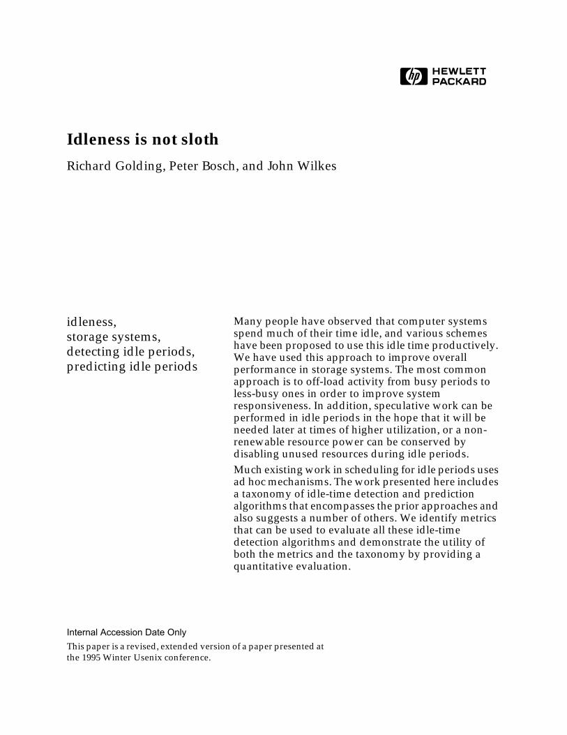
Figure 1 shows the overall structure of the framework of the idle detection system we haveinvestigated. Foreground work requests arrive and are executed, requiring resources. Potentiallyuseful idle tasks also consume the same resources. An idleness detector monitors the foreground-work arrivals and the state of the scheduler, and many detector algorithms use the recent historyof these events to guide their predictions of idle time. The detector can also considerenvironmental factors such as time of day. The idleness detector gives its predictions to theactuator, which schedules the background idle work.

Figure 1: the idle-time processing framework.

foregroundwork

idlenessdetector resource

predictions

scheduler

background idle work

environment

actuator

load

1

The goal of the idleness detector is to make sufficiently good predictions that the net effect to thesystem of running the idle task is positive. The best predictions exploit all the idle time and makeno mistaken predictions.

There are two basic ways to measure how good an idle-time processing system is. Externalmeasures quantify the interference between the idle task and an outside application, and thebenefit from running the idle task. They use units such as additional foreground operation latencyor power consumption. Internal measures are based solely on how accurate the detector’spredictions are. The external measures are what really matter, but internal measures are easy toobtain and can be useful for guiding the choice of detection mechanism.

The rest of this paper is organized as follows. The rest of this section discusses some of thecharacteristics of the idle periods in storage systems we have investigated. The following sectionlooks at several aspects of the problem of making good predictions about this idle time, includinga discussion of how they can be measured. We then present an architecture and taxonomy foridleness detectors, use this taxonomy as a tool to generate a suite of idleness detectors, andevaluate their effectiveness under realistic, measured workloads. An analysis of the effectivenessof the taxonomy and an investigation of how one can choose an idleness detector follow. Somethoughts about opportunities for future work and our conclusions wrap up the paper.

1.1 The nature of idle timeIn our research, we have analyzed traces of storage operations taken from a number of systems,including file systems, databases, and RAID arrays. We will be presenting results from tracestaken from file system disks attached to HP-UX systems. Details on most of these traces can befound in our earlier paper on modeling disk systems [Ruemmler93].

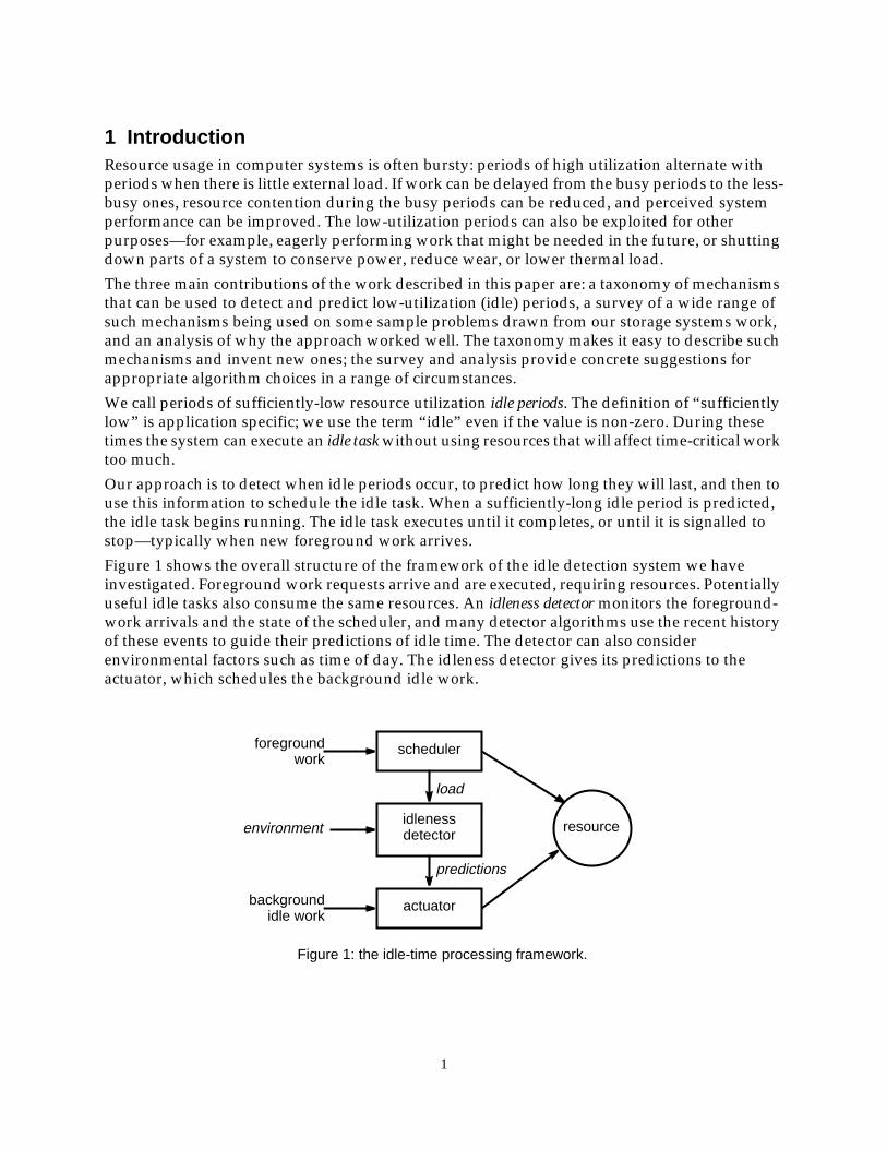
Most idle periods in these traces are very short—on the order of milliseconds—but the bulk of idletime comes from a few very long periods. (Figure 2 shows one such distribution.) This means that

0.0001 0.001 0.01 0.1 1 10 100 1000

Duration (seconds)

0.0

0.2

0.4

0.6

0.8

1.0

Cum

ulat

ive

frac

tion

TimeCount

Figure 2: cumulative distribution of idle time as a function of idle periodduration, for the cello-disk6 trace. The upper curve shows the fraction of thenumber of idle periods; the lower curve shows the fraction of total idle time.

2

a system that uses idle time can get most of the benefit by doing a good job of finding the long idleperiods.

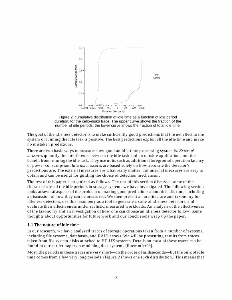
Idle periods also exhibit predictable patterns. To determine this, we computed the autocorrelationfor the sequence of idle period lengths. Figure 3 shows the results: for most of the traces weinvestigated, how long the system stays idle is strongly related to how long it has recently beenidle. The figure shows the three patterns we observed among the traces.

• hplajw-disk0: this trace was taken on a quiet personal workstation. Most of the idle periodswere very long, and there was strong correlation between the length of one period and thelengths of the preceding periods.

• cello-disk6: this trace is from a disk holding the Usenet news partition on a time-sharingsystem. The length of time the system stayed idle depended only on the four previousperiods, and there appeared to be little longer-term correlation.

• database-disk0: this disk held part of a large production database system that exhibited atransaction-processing-like workload. As with the cello-disk6 trace, the lengths of theprevious few idle periods are strongly correlated with the length of the current one, butthere are also long-term correlations at lags of more than forty periods.

Other researchers have indicated that file system traffic exhibits self-similar behavior [Gribble96].In particular, they have shown that there is substantial long-term dependence between thedurations of idle periods.

These results suggest that idleness is a predictable phenomenon: by observing recent behavior,and using the dependence between recent and future events, one can make good predictionsabout future behavior.

2 An overview of idle-time processingIdle-time processing consists, first, of detecting an idle period, then using that knowledge toexecute idle tasks to benefit overall system performance. In this section we explain what we meanby each of these things.

0 10 20 30 40 50

lag (periods)

0.2

0.4

0.6

0.8

1.0

auto

corre

latio

n

hplajw-disk0

0 10 20 30 40 50

lag (periods)

0.0

0.5

1.0

auto

corre

latio

n

cello-disk6

0 10 20 30 40 50

lag (periods)

0.0

0.5

1.0

auto

corre

latio

n

database-disk0

Figure 3: autocorrelation at different lags of the sequence of idle period duration, for threeworkloads. Dark bars indicate significant correlation at 95% confidence level.

3

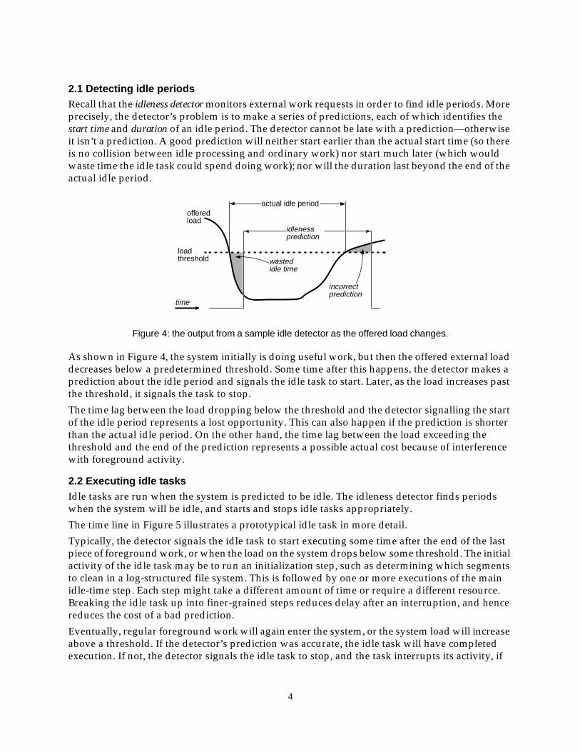
2.1 Detecting idle periodsRecall that the idleness detector monitors external work requests in order to find idle periods. Moreprecisely, the detector’s problem is to make a series of predictions, each of which identifies thestart time and duration of an idle period. The detector cannot be late with a prediction—otherwiseit isn’t a prediction. A good prediction will neither start earlier than the actual start time (so thereis no collision between idle processing and ordinary work) nor start much later (which wouldwaste time the idle task could spend doing work); nor will the duration last beyond the end of theactual idle period.

As shown in Figure 4, the system initially is doing useful work, but then the offered external loaddecreases below a predetermined threshold. Some time after this happens, the detector makes aprediction about the idle period and signals the idle task to start. Later, as the load increases pastthe threshold, it signals the task to stop.

The time lag between the load dropping below the threshold and the detector signalling the startof the idle period represents a lost opportunity. This can also happen if the prediction is shorterthan the actual idle period. On the other hand, the time lag between the load exceeding thethreshold and the end of the prediction represents a possible actual cost because of interferencewith foreground activity.

2.2 Executing idle tasksIdle tasks are run when the system is predicted to be idle. The idleness detector finds periodswhen the system will be idle, and starts and stops idle tasks appropriately.

The time line in Figure 5 illustrates a prototypical idle task in more detail.

Typically, the detector signals the idle task to start executing some time after the end of the lastpiece of foreground work, or when the load on the system drops below some threshold. The initialactivity of the idle task may be to run an initialization step, such as determining which segmentsto clean in a log-structured file system. This is followed by one or more executions of the mainidle-time step. Each step might take a different amount of time or require a different resource.Breaking the idle task up into finer-grained steps reduces delay after an interruption, and hencereduces the cost of a bad prediction.

Eventually, regular foreground work will again enter the system, or the system load will increaseabove a threshold. If the detector’s prediction was accurate, the idle task will have completedexecution. If not, the detector signals the idle task to stop, and the task interrupts its activity, if

time

Figure 4: the output from a sample idle detector as the offered load changes.

offeredload

loadthreshold

actual idle period

incorrectprediction

wastedidle time

idlenessprediction

4

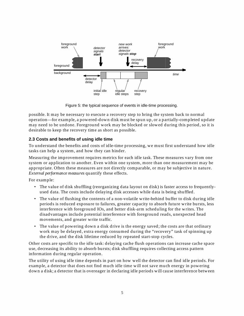
possible. It may be necessary to execute a recovery step to bring the system back to normaloperation—for example, a powered-down disk must be spun up, or a partially-completed updatemay need to be undone. Foreground work may be blocked or slowed during this period, so it isdesirable to keep the recovery time as short as possible.

2.3 Costs and benefits of using idle timeTo understand the benefits and costs of idle-time processing, we must first understand how idletasks can help a system, and how they can hinder.

Measuring the improvement requires metrics for each idle task. These measures vary from onesystem or application to another. Even within one system, more than one measurement may beappropriate. Often these measures are not directly comparable, or may be subjective in nature.External performance measures quantify these effects.

For example:

• The value of disk shuffling (reorganizing data layout on disk) is faster access to frequently-used data. The costs include delaying disk accesses while data is being shuffled.

• The value of flushing the contents of a non-volatile write-behind buffer to disk during idleperiods is reduced exposure to failures, greater capacity to absorb future write bursts, lessinterference with foreground IOs, and better disk-arm scheduling for the writes. Thedisadvantages include potential interference with foreground reads, unexpected headmovements, and greater write traffic.

• The value of powering down a disk drive is the energy saved; the costs are that ordinarywork may be delayed, extra energy consumed during the “recovery” task of spinning upthe drive, and the disk lifetime reduced by repeated start-stop cycles.

Other costs are specific to the idle task: delaying cache flush operations can increase cache spaceuse, decreasing its ability to absorb bursts; disk shuffling requires collecting access patterninformation during regular operation.

The utility of using idle time depends in part on how well the detector can find idle periods. Forexample, a detector that does not find much idle time will not save much energy in poweringdown a disk; a detector that is overeager in declaring idle periods will cause interference between

foregroundwork

Figure 5: the typical sequence of events in idle-time processing.

detectordelay

detectorsignalsstart

new workarrives:detectorsignals stop

recoverydelay

foregroundwork

regularidle steps

initial idlestep

recoverystep

time

foreground

background

5

background and foreground work. Thus the internal measures of detector performance can helpexplain why one detector works better than another for some systems.

2.4 Characterizing idle tasksThere are many different uses for idle time, but they mostly fall into four different categories:

• Required work that can be delayed, such as delayed cache writes, migrating objects in a storagehierarchy, rebuilding a RAID array after a failure, cleaning a log-structured file system.

• Work that will probably be requested later, such as disk readahead, eager function evaluation,collapsing chains of forwarding addresses for mobile objects, eager make [Bubenik89].

• Work that is not necessary, but will improve system behavior, such as rearranging data layout ondisk, shutting down parts of a system to conserve power, checking system integrity,compressing unused data.

• Shifting work from a busy to an idle resource, such as choosing the least-loaded network path,compressing data to reduce disk or network traffic.

Idle tasks can also be characterized by how they react to being stopped and started (we call thesegranularity properties):

• Interruptability: some idle tasks can be interrupted at any time, and will stop immediately.Others must complete a fixed granule of work before they can relinquish the systemresources they are consuming. (For example, a disk write operation must run to completion,while a powered-down device can be restarted at any time.)

• Work loss: when some idle tasks are interrupted, they will lose or must discard some of thework that they have performed. (For example a log-structured file system cleaner may haveto abandon work on the current segment.) This cleanup process itself may need resources,and some idle tasks have to be followed by a recovery task to put the system back to aconsistent state.

• Resource use: most idle tasks block foreground work from making progress to some degree.In the extreme, they may completely deny foreground-work access to a resource (e.g., a diskthat has been spun down); in other cases, foreground activity simply slows down while theidle task is executing.

Each of these properties affects applications in different ways. For example, high degrees ofmultiprogramming will probably make a workload more resilient to an idle task that blocksaccess to a single resource, since there is probably something else useful that can be done whilethe idle task has the resource.

2.5 Idle task examplesThere are many possible uses for idle time. Storage, compilation, user interfaces, and distributedsystems all exhibit highly variable workloads—a clue that a system could benefit from idle-timeprocessing. We surveyed a number of them in an earlier paper [Golding95]. Here we present threeexamples that we will use throughout this paper, together with how our taxonomy classifiesthem.

2.5.1 Disk power-downSeveral people have investigated powering down disk drives on portable computers to conserveenergy (e.g., [Cáceres93, Douglis95, Greenawalt94, Marsh93, Wilkes92b]). Using the taxonomy

6

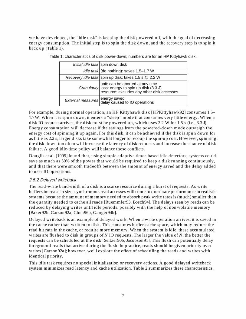
we have developed, the “idle task” is keeping the disk powered off, with the goal of decreasingenergy consumption. The initial step is to spin the disk down, and the recovery step is to spin itback up (Table 1).

For example, during normal operation, an HP Kittyhawk disk [HPKittyhawk92] consumes 1.5–1.7W. When it is spun down, it enters a “sleep” mode that consumes very little energy. When adisk IO request arrives, the disk must be powered up, which uses 2.2 W for 1.5 s (i.e., 3.3 J).Energy consumption will decrease if the savings from the powered-down mode outweigh theenergy cost of spinning it up again. For this disk, it can be achieved if the disk is spun down foras little as 2.2 s; larger disks take somewhat longer to recoup the spin-up cost. However, spinningthe disk down too often will increase the latency of disk requests and increase the chance of diskfailure. A good idle-time policy will balance these conflicts.

Douglis et al. [1995] found that, using simple adaptive timer-based idle detectors, systems couldsave as much as 50% of the power that would be required to keep a disk running continuously,and that there were smooth tradeoffs between the amount of energy saved and the delay addedto user IO operations.

2.5.2 Delayed writebackThe read-write bandwidth of a disk is a scarce resource during a burst of requests. As writebuffers increase in size, synchronous read accesses will come to dominate performance in realisticsystems because the amount of memory needed to absorb peak write rates is (much) smaller thanthe quantity needed to cache all reads [Ruemmler93, Bosch94]. The delays seen by reads can bereduced by delaying writes until idle periods, possibly with the help of non-volatile memory[Baker92b, Carson92a, Chen96b, Ganger94b].

Delayed writeback is an example of delayed work. When a write operation arrives, it is saved inthe cache rather than written to disk. This consumes buffer-cache space, which may reduce theread hit rate in the cache, or require more memory. When the system is idle, these accumulatedwrites are flushed to disk in groups of N IO requests. The larger the value of N, the better therequests can be scheduled at the disk [Seltzer90b, Jacobson91]. This flush can potentially delayforeground reads that arrive during the flush. In practice, reads should be given priority overwrites [Carson92a]; however, we’ll explore the effect of scheduling the reads and writes withidentical priority.

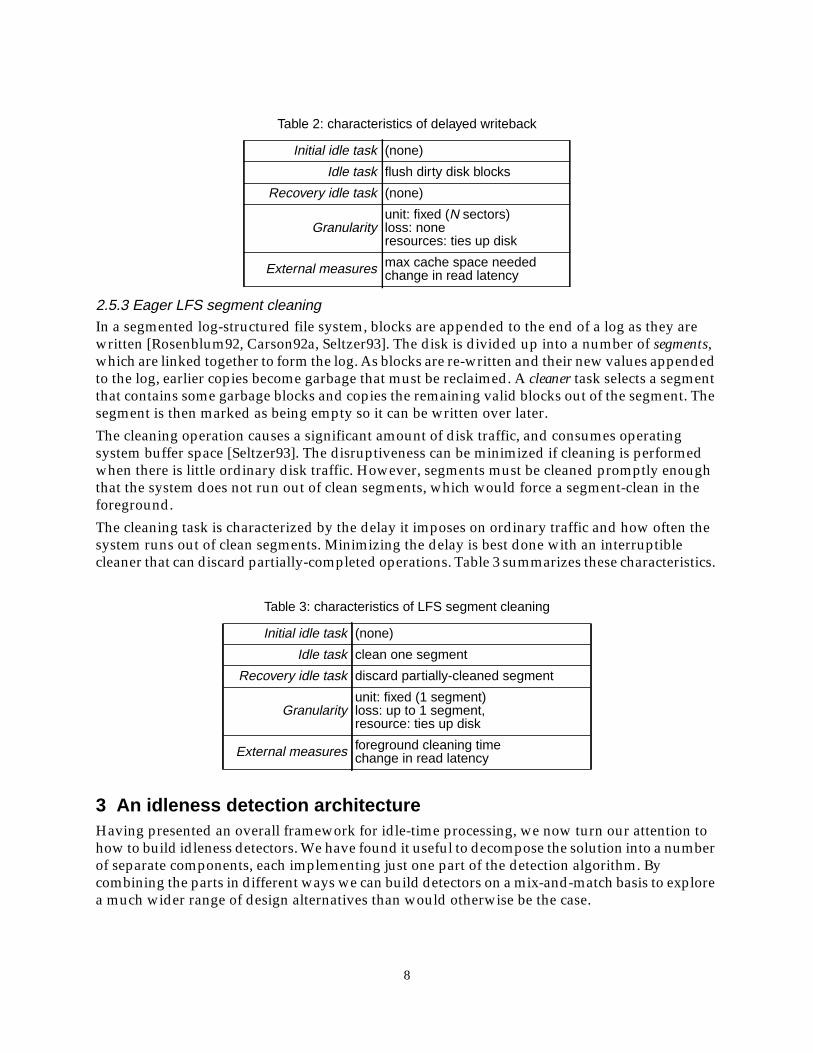
This idle task requires no special initialization or recovery actions. A good delayed writebacksystem minimizes read latency and cache utilization. Table 2 summarizes these characteristics.

Table 1: characteristics of disk power-down; numbers are for an HP Kittyhawk disk.

Initial idle task spin down disk

Idle task (do nothing): saves 1.5–1.7 W

Recovery idle task spin up disk: takes 1.5 s @ 2.2 W

Granularityunit: can be aborted at any timeloss: energy to spin up disk (3.3 J)resource: excludes any other disk accesses

External measures energy saveddelay caused to IO operations

7

2.5.3 Eager LFS segment cleaningIn a segmented log-structured file system, blocks are appended to the end of a log as they arewritten [Rosenblum92, Carson92a, Seltzer93]. The disk is divided up into a number of segments,which are linked together to form the log. As blocks are re-written and their new values appendedto the log, earlier copies become garbage that must be reclaimed. A cleaner task selects a segmentthat contains some garbage blocks and copies the remaining valid blocks out of the segment. Thesegment is then marked as being empty so it can be written over later.

The cleaning operation causes a significant amount of disk traffic, and consumes operatingsystem buffer space [Seltzer93]. The disruptiveness can be minimized if cleaning is performedwhen there is little ordinary disk traffic. However, segments must be cleaned promptly enoughthat the system does not run out of clean segments, which would force a segment-clean in theforeground.

The cleaning task is characterized by the delay it imposes on ordinary traffic and how often thesystem runs out of clean segments. Minimizing the delay is best done with an interruptiblecleaner that can discard partially-completed operations. Table 3 summarizes these characteristics.

3 An idleness detection architectureHaving presented an overall framework for idle-time processing, we now turn our attention tohow to build idleness detectors. We have found it useful to decompose the solution into a numberof separate components, each implementing just one part of the detection algorithm. Bycombining the parts in different ways we can build detectors on a mix-and-match basis to explorea much wider range of design alternatives than would otherwise be the case.

Table 2: characteristics of delayed writeback

Initial idle task (none)

Idle task flush dirty disk blocks

Recovery idle task (none)

Granularityunit: fixed (N sectors)loss: noneresources: ties up disk

External measures max cache space neededchange in read latency

Table 3: characteristics of LFS segment cleaning

Initial idle task (none)

Idle task clean one segment

Recovery idle task discard partially-cleaned segment

Granularityunit: fixed (1 segment)loss: up to 1 segment,resource: ties up disk

External measures foreground cleaning timechange in read latency

8

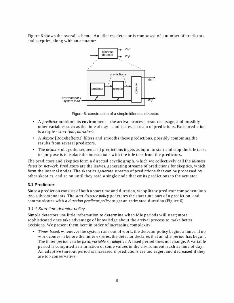
Figure 6 shows the overall scheme. An idleness detector is composed of a number of predictorsand skeptics, along with an actuator:

• A predictor monitors its environment—the arrival process, resource usage, and possiblyother variables such as the time of day—and issues a stream of predictions. Each predictionis a tuple <start time, duration>.

• A skeptic [Rodeheffer91] filters and smooths these predictions, possibly combining theresults from several predictors.

• The actuator obeys the sequence of predictions it gets as input to start and stop the idle task;its purpose is to isolate the interactions with the idle task from the predictors.

The predictors and skeptics form a directed acyclic graph, which we collectively call the idlenessdetection network. Predictors are the leaves, generating streams of predictions for skeptics, whichform the internal nodes. The skeptics generate streams of predictions that can be processed byother skeptics, and so on until they read a single node that emits predictions to the actuator.

3.1 PredictorsSince a prediction consists of both a start time and duration, we split the predictor component intotwo subcomponents. The start detector policy generates the start time part of a prediction, andcommunicates with a duration predictor policy to get an estimated duration (Figure 6).

3.1.1 Start time detector policySimple detectors use little information to determine when idle periods will start; moresophisticated ones take advantage of knowledge about the arrival process to make betterdecisions. We present them here in order of increasing complexity.

• Timer-based: whenever the system runs out of work, the detector policy begins a timer. If nowork comes in before the timer expires, the detector declares that an idle period has begun.The timer period can be fixed, variable, or adaptive. A fixed period does not change. A variableperiod is computed as a function of some values in the environment, such as time of day.An adaptive timeout period is increased if predictions are too eager, and decreased if theyare too conservative.

Figure 6: construction of a simple idleness detector.

idlenessdetector

start

stop

environment +system load

start

stopactuator

skepticpredictor

predictions

9

• Rate-based: the detector policy maintains an estimate of the rate at which work is arriving,and declares an idle period when its rate estimate falls below a threshold. Differentthreshold rates can be used for “start of idle period” and “end of idle period” to providesome hysteresis. Methods for maintaining the estimate include:– moving average: the rate is periodically sampled, and the detector computes a moving

average of the samples.– event window: the detector maintains the times of the last n arrivals, and estimates the rate

as n divided by the age of the oldest arrival. This is similar to leaky bucket rate-controlschemes for high-speed networks [Cruz92].

– time window: the predictor maintains a list of arrival times more recent than t seconds,and estimates the rate as the length of the list divided by t. This is a variation on the eventwindow method.

– adaptive: like the other rate-based policies, but the threshold rates are adapted based onthe accuracy of recent predictions in order to meet an accuracy goal.

• Rate-change-based: these predictors maintain an estimate of the first derivative of the arrivalrate to predict in advance when the arrival rate will fall below a threshold.

• Periodic: if the workload contains work that repeats with a nearly constant period, a digitalphase locked loop or DPLL [Lindsey81, Massalin89a] can be used to synchronize predictionsto these periodic events in the workload. By knowing when work will arrive, such as a file-system daemon that does periodic buffer-cache flushes, the idle periods can also bepredicted.

3.1.2 Duration prediction policyA wide range of techniques can be used to adapt an estimate of how long an idle period will lastto a changing workload. We list them here according to the amount of information they use aboutthe arrival process.

• No duration: no prediction is made (alternately, the prediction is “forever”). Variants on thisapproach include policies that merely detect the end of an idle period when it happens,rather than making a prediction beforehand. These are most useful when the definition of“idle” allows some residual foreground work.

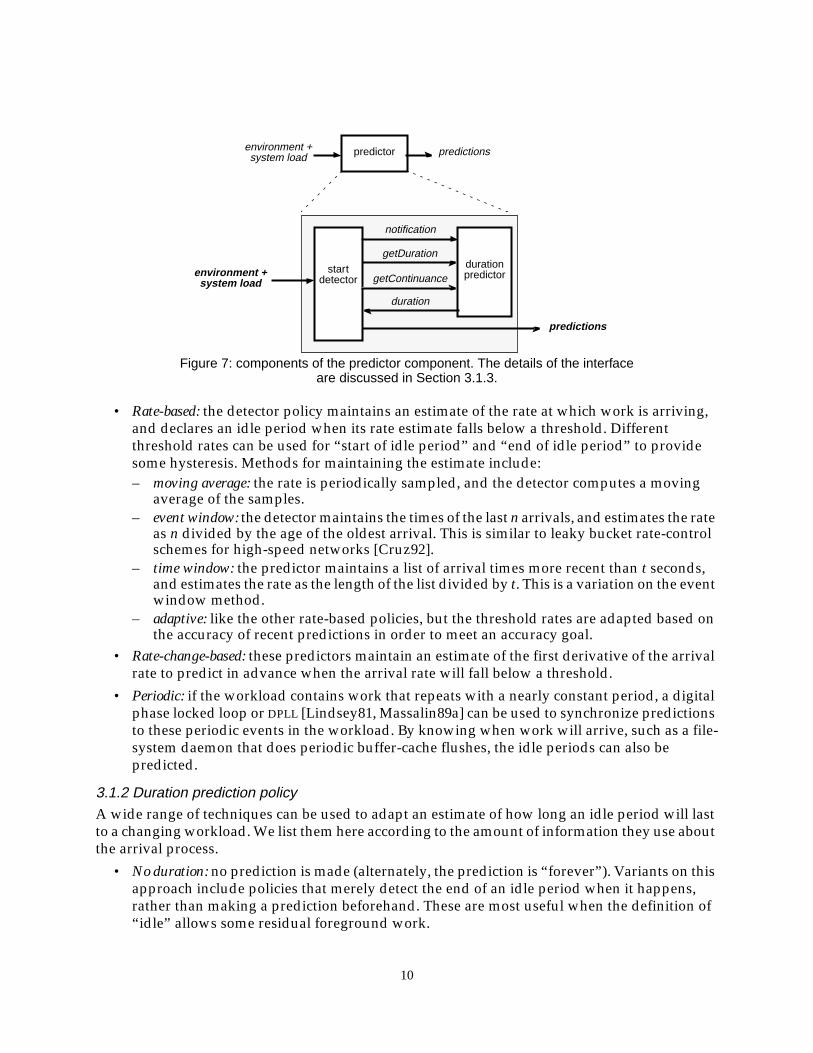
Figure 7: components of the predictor component. The details of the interfaceare discussed in Section 3.1.3.

predictorenvironment +system load

startdetector

predictions

predictions

durationpredictorenvironment +

system load getContinuance

duration

notification

getDuration

10

• Fixed duration: a fixed duration is predicted. The simplest form of this is “enough time to runthe idle task once”.

• Moving average: the duration prediction policy keeps a moving (possibly weighted) averageof the actual durations. The usual average is the mean, but a geometric average or mediancan also be used. (More generally, the predictor can treat idle periods as an ARIMA process[Box94].)

• Filtered moving average: like moving average, but only idle periods greater than some lower-bound are considered during the averaging process, so that the presence of many very shortidle periods that cannot be used does not bias the results for longer, useful periods.

• Backoff: after each prediction is used, the duration predictor uses the feedback to determinewhether the actual duration was longer or shorter than predicted. If it was longer, the nextprediction is increased; if it was shorter, the next prediction is decreased. The increases can

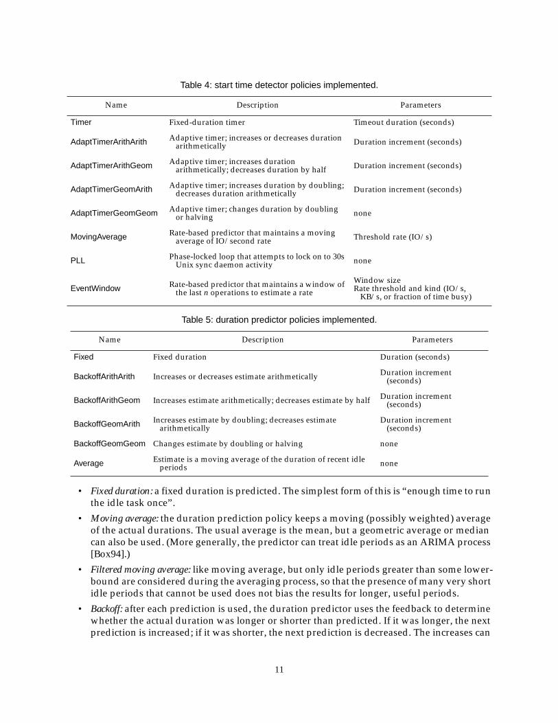
Table 4: start time detector policies implemented.

Name Description Parameters

Timer Fixed-duration timer Timeout duration (seconds)

AdaptTimerArithArith Adaptive timer; increases or decreases durationarithmetically Duration increment (seconds)

AdaptTimerArithGeom Adaptive timer; increases durationarithmetically; decreases duration by half Duration increment (seconds)

AdaptTimerGeomArith Adaptive timer; increases duration by doubling;decreases duration arithmetically Duration increment (seconds)

AdaptTimerGeomGeom Adaptive timer; changes duration by doublingor halving none

MovingAverage Rate-based predictor that maintains a movingaverage of IO/second rate Threshold rate (IO/s)

PLL Phase-locked loop that attempts to lock on to 30sUnix sync daemon activity none

EventWindow Rate-based predictor that maintains a window ofthe last n operations to estimate a rate

Window sizeRate threshold and kind (IO/s,

KB/s, or fraction of time busy)

Table 5: duration predictor policies implemented.

Name Description Parameters

Fixed Fixed duration Duration (seconds)

BackoffArithArith Increases or decreases estimate arithmetically Duration increment(seconds)

BackoffArithGeom Increases estimate arithmetically; decreases estimate by half Duration increment(seconds)

BackoffGeomArith Increases estimate by doubling; decreases estimatearithmetically

Duration increment(seconds)

BackoffGeomGeom Changes estimate by doubling or halving none

Average Estimate is a moving average of the duration of recent idleperiods none

11

be arithmetic, increasing by a constant each time, or geometric, increasing by a constantfactor. The skeptic in Autonet [Rodeheffer91] and round-trip timers in TCP [Postel80a,Comer91, Karn91] used geometric increase and arithmetic decrease to maintain a predictionslightly longer than the actual, while a duration predictor works to keep its predictionsslightly shorter.

The backoff algorithm can be applied either at the end of the prediction period or at the endof the idle period. The first gives a chance for the algorithm to be much more aggressive inextending its estimates; the latter provides more information, but potentially causes theperiod to be adjusted much less often.

• Filtered backoff: backoff policies that only consider actual idle periods longer than a givenlower-bound during their backoff calculations.

• Autocorrelation: the autocorrelation on the work arrival process gives the probability of anevent arriving or the rate of arrival as a function of time into the future. The predictedduration is the period during which the probability of arrival is below some threshold. Theautocorrelation is somewhat expensive to compute, so it might be recomputed periodicallyrather than continuously. It might also be used to predict the beginning of multiple idleperiods.

• Conditional autocorrelation: like a simple autocorrelation, except that multipleautocorrelation functions are computed based on some property of arriving events. Forexample, the expected future might be different following read requests or write requests.

• Ad-hoc rules: finally, as with predicting the beginning of an idle period, many systems cantake advantage of other specific features of the arrival process, such as periodicity.

3.1.3 Interface between start time and duration prediction policiesIn our evaluations, we separated the implementation of the start detector policy from that ofduration prediction policy, as shown in Figure 6.

The interface between the two policies required a few revisions to get right. The final versionconsisted of three parts:

1. Notifications of the beginning and ending of actual idle periods sent from the start detectorto the duration predictor.

2. Requests from the start detector for a duration prediction at the beginning of an idle period.We called this operation getDuration.

3. Requests for a duration prediction in the middle of an idle period, called getContinuance.

Predicting duration of an idle period that is in progress is necessary because many periods runmuch longer than initially predicted, and it can be useful to get a prediction of how much longerit will likely continue, given that it has already lasted at least as long as the original prediction.

3.1.4 Offline predictorsAs with so many problems of this type, optimal idleness detection requires off-line analysis thathas knowledge of future events. While this approach is often not useful for building a system, inthose cases where usage patterns are stable a one-time analysis may provide a useful prediction.For example, “weekends from 1–6 a.m.” is a common time to perform system maintenance.

In practice, however, we have concentrated on on-line detectors for our work.

12

3.2 SkepticsA skeptic takes in one or more prediction streams, and emits a new one. Skeptics are used to filterout bad predictions and to combine the results from several predictors into a single predictionstream.

Single-stream (filtering) skeptics include:

• low-pass: discards predicted periods that are shorter than some threshold (e.g., the durationof the idle task).

• quality: discards predictions from a predictor that is consistently wrong. The skeptic cancompute a measure of the predictor’s accuracy, perhaps filtered to remove short-termvariations, and pass along predictions when the accuracy is above some threshold.

• environmental: discards or modifies predictions according to some external event (such astime of day). This can allow idleness predictions to be restricted to times when nobody isaround, for example. The time-of-day input can be derived from moving averages ofworkloads over long periods of time, so this skeptic can be made adaptive.

Perhaps the most important use for skeptics is to combine several prediction streams. Forexample, a periodic-work detector will not handle non-periodic bursts, while another predictormight. A skeptic could combine the two, only reporting a prediction when both agree.

More generally, a skeptic can combine a number of input streams by weighted voting. Eachstream is given a weight, and the skeptic produces a prediction only when the combined weightsare greater than some threshold. When the weights are equal and fixed, this becomes simplevoting. Alternately, the weights can be varied according to the accuracy of each predictor. Thisapproach has been shown to yield near-optimal prediction in many cases [CesaBianchi94].

3.3 ActuatorThe actuator uses the stream of predictions provided by the network of predictors and skeptics tosignal idle tasks to start and stop. When the actuator signals an idle task to start running, it canpass along an indication of how long the prediction network expects the system to stay idle. Someof the idle tasks we evaluated used the prediction to scale the amount of work they tried to do.

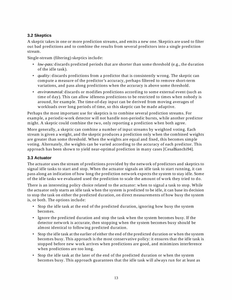
There is an interesting policy choice related to the actuator: when to signal a task to stop. Whilethe actuator only starts an idle task when the system is predicted to be idle, it can base its decisionto stop the task on either the predicted duration, on direct measurements of how busy the systemis, or both. The options include:

• Stop the idle task at the end of the predicted duration, ignoring how busy the systembecomes.

• Ignore the predicted duration and stop the task when the system becomes busy. If thedetector network is accurate, then stopping when the system becomes busy should bealmost identical to following predicted duration.

• Stop the idle task at the earlier of either the end of the predicted duration or when the systembecomes busy. This approach is the most conservative policy: it ensures that the idle task isstopped before new work arrives when predictions are good, and minimizes interferencewhen predictions are too long.

• Stop the idle task at the later of the end of the predicted duration or when the systembecomes busy. This approach guarantees that the idle task will always run for at least as

13

long as it was told in the prediction, and longer if possible. It is, however, the leastconservative, and we have not yet found a use for it.

4 Experimental resultsTo get quantitative measures of the effectiveness of idle-time processing, we used the taxonomypresented in Section 3 to design and implement a large number of possible idleness detectionnetwork components and networks composed from them, whose performance we thenevaluated.

We used three idle tasks, as detailed in Section 2.5. They were:

• disk power-down: spin down an idle disk drive to save power;

• delayed writeback: delay disk write operations to idle periods; and

• eager segment cleaning: perform LFS segment cleaning when there is little other traffic.

We begin this section with a discussion of the methods we used in the evaluation, and then studyeach of the three idle tasks in turn.

4.1 MethodologyWe implemented our idle processing architecture in the Pantheon simulation system [Wilkes95].In particular, we simulated a host system issuing read and write requests to a set of disks. Weused calibrated disk models [Ruemmler94], and exercised our detectors using week-long IOaccess traces taken from three real systems [Ruemmler93] to avoid making simplifyingassumptions about access rates or patterns:

• hplajw: a trace of a single-user HP 9000/845 workstation with two 300MB disks.

• snake: a trace of a HP 9000/720 file server at UC Berkeley with three disks—one 500MB andtwo 1.35GB.

• cello: a trace of the eight disks on an HP 9000/877 cluster server. We often report on cello-disk6, which held the /news partition and accounted for about half the IO traffic in thesystem.

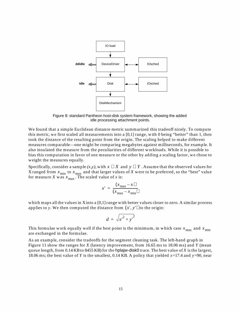
The Pantheon simulator uses the system model shown in Figure 8. We used an open queuingmodel, where IO events were replayed according to the times recorded in the trace. To providesupport for idleness detection, we modified the DeviceDriver and Disk classes to let us connectidleness detector networks. The delayed writeback and segment cleaning tasks used events fromthe device driver level, while the powerdown task used events from the disk controller.

4.1.1 Measures used for evaluationWe used two analytical techniques in our evaluation that bear discussion. The first summarizesthe tradeoff between two otherwise incomparable measures. The second measures theconsistency of a measure across multiple workloads.

All three of the idle tasks we modeled present tradeoffs among multiple measures. The segmentcleaning task, for example, balanced aggressive cleaning to keep the amount of unprocessed datalow against conservative cleaning to minimize the interference with foreground operations. Theideal was to minimize both the amount of unprocessed data and the interference: a policy thatyielded moderately good performance at both measures is better than a policy that yields lowunprocessed data at the cost of very high interference.

14

We found that a simple Euclidean distance metric summarized this tradeoff nicely. To computethis metric, we first scaled all measurements into a [0,1] range, with 0 being “better” than 1, thentook the distance of the resulting point from the origin. The scaling helped to make differentmeasures comparable—one might be comparing megabytes against milliseconds, for example. Italso insulated the measure from the peculiarities of different workloads. While it is possible tobias this computation in favor of one measure or the other by adding a scaling factor, we chose toweight the measures equally.

Specifically, consider a sample (x,y), with and . Assume that the observed values forX ranged from to and that larger values of X were to be preferred, so the “best” valuefor measure X was . The scaled value of x is:

which maps all the values in X into a [0,1] range with better values closer to zero. A similar processapplies to y. We then computed the distance from to the origin:

This formulae work equally well if the best point is the minimum, in which case andare exchanged in the formulae.

As an example, consider the tradeoffs for the segment cleaning task. The left-hand graph inFigure 11 show the ranges for X (latency improvement, from 16.65 ms to 18.06 ms) and Y (meanqueue length, from 0.14 KB to 8455 KB) for the hplajw-disk0 trace. The best value of X is the largest,18.06 ms; the best value of Y is the smallest, 0.14 KB. A policy that yielded x=17.4 and y=90, near

IO load

Figure 8: standard Pantheon host-disk system framework, showing the addedidle processing attachment points.

ddidle

idle

DeviceDriver

DiskMechanism

IOsched

IOsched

Disk

x X∈ y Y∈xmin xmax

xmax

x'xmax x–( )

xmax xmin–( )--------------------------------=

x' y',( )

d x'2 y+ '

2=

xmax xmin

15

the center of the graph, would be scaled to and. The distance metric is

We also wanted to determine how consistently various policies performed across differentworkloads. A measure of consistency should indicate whether one policy consistently yieldedbetter results than another policy across several workloads. It should also indicate whether asingle policy produced equally good results across workloads. We used these indications tosuggest policies that are generally safe choices over a wide range of conditions.

Our approach to defining a consistency metric was to use the mean and variance of how well eachpolicy did across the workloads. We first scaled all the results for a particular workload into a (0,1)range just as we did for the distance metric. The mean of this measure for one detector acrossmultiple workloads indicates how close to the best value the detector was, on average, and thevariance of the measure indicates how consistent the results were.

More formally, consider a set of measurements taken by using a set of policies P witha set of workloads W. For each workload , we can find the best and worst values for eachworkload w, and , and compute range of values . Foreach policy , the scaled measure is

This scaled measure can be thought of as the fraction that policy p produced of the best result forworkload w. The mean,

gives the overall “goodness”, and allows us to compare two policies; the variance of this measureindicates whether the policy performance varied across different workloads or not.

4.2 Disk power-downThe first idle task we looked at was disk power-down, which tries to save energy by turning offa disk drive when it is not being used, as discussed in Section 2.5.1.

There were two external measures we used to evaluate the disk power-down idle task: the energysaved, and the number of operations that had to be delayed because the disk wasn’t ready whenthe operation was issued. These are similar to the measures that have been considered in otherstudies on this problem [Douglis95].

In our model, the idleness detection network monitored activity inside the disk controller. Eachdisk was augmented to include an idleness detection network and an idle task. The idle taskinitiated a spindown whenever it received a prediction from the detection network, and waitedto spin the disk back up until a disk IO request arrived.

Real disks have a great many different power-management systems. We used a simple,representative power management system derived from typical 2.5” disks. We assumed that thedisk would require 1 s to spin down and 1.5 s to spin up. It would consume 1.6 W during normal

x' 18.06 17.4–( ) 18.06 16.65–( )⁄ 0.46= =y 0.14 90–( ) 0.14 8455–( )⁄ 0.0106= =

d 0.46( )2 0.0106( )2+ 0.46012= =

mp w, M∈w W∈

mbest w, mworst w, rw mbest w, mworst w,–=p P∈

m'p w,mbest w, mp w,–( )

rw-----------------------------------------=

m'p1W-------- m'p w,

w W∈∑=

16

operation; 0.4 W while sleeping; and 2.4 W while spinning up. For these parameters, the break-even point, where the energy saved while being spun down equals the energy cost of spinningback up, is 3 s.

For the idle detection networks, we evaluated each of our start time detectors combined with aFixed 10 s duration predictor—this being what we considered a reasonable minimum duration.The fixed duration predictor provided a target for the adaptive start time detectors: whenworking properly, they adapted their detection policy to only declare idleness when it was likelythat the system would stay idle for at least long enough to save a little power.

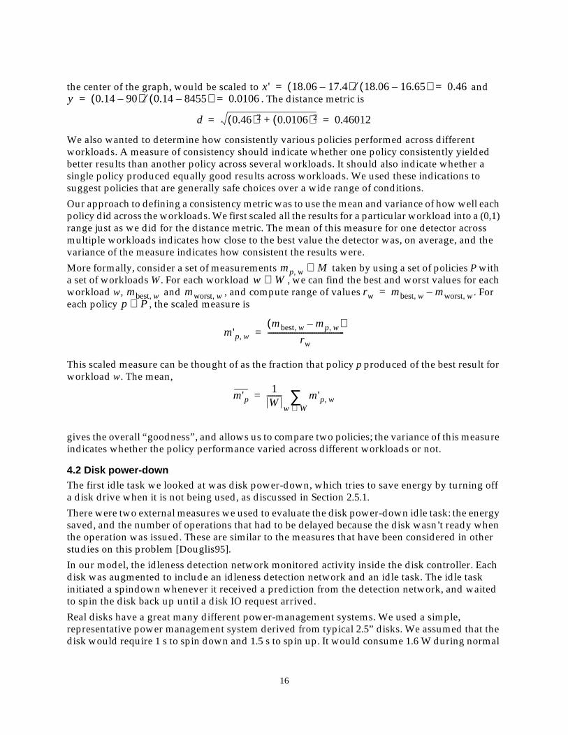
Figure 9 shows the detailed results for two of the disk traces we evaluated, comparing the powersaved against the number of delayed operations. Note that higher power savings and fewerdelayed operations is to be preferred, which is to the lower right in the graph. The small graphsshow how each family of start time detection policies performed compared to the overall picture.

There is a clear tradeoff between the two measures. In our implementation, at least one operationwas delayed every time the disk was powered up because the disk never tried to anticipate whenfuture requests might arrive. Detectors that powered down the disk more often therefore delayedthe most operations, and indeed for all but three disks in the traces the two measures arecorrelated at a 95% likelihood. The three exceptions came from disks where the PLL detectorsaved relatively little power but still delayed many operations. (The sample in the lower left ofboth graphs in Figure 9 is from a PLL detector.)

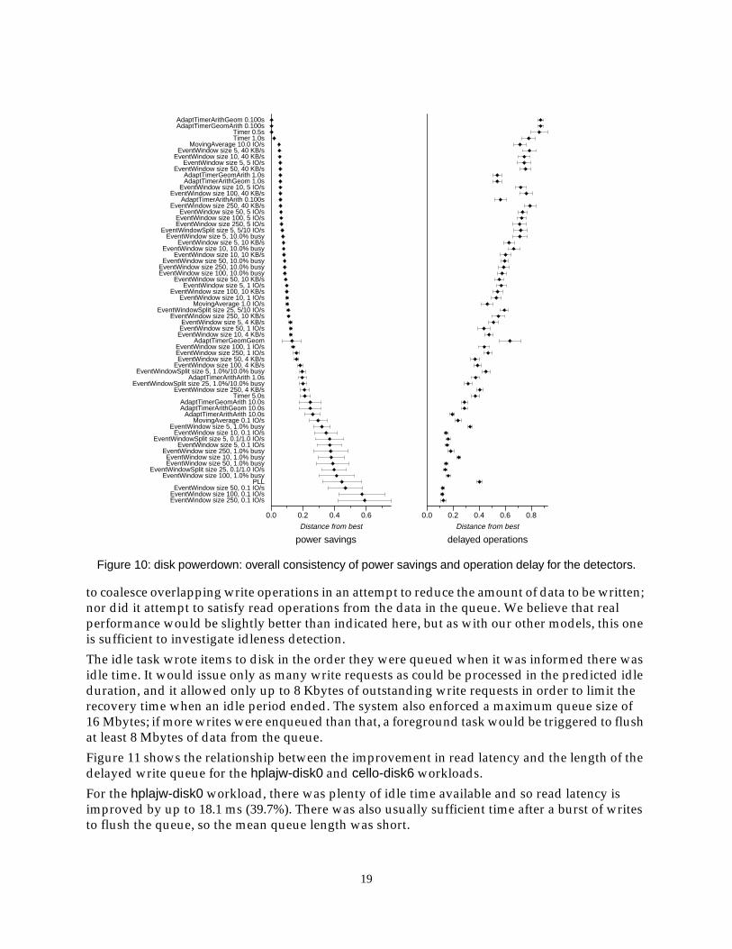
For power savings, a few start detectors consistently did the best over the 13 disks in ourworkload traces, as shown in on the left-hand side of Figure 10. The AdaptTimerArithGeom 0.1sand 1.0s and Timer 0.5s and 1.0s appear to be the four safest choices: they get within 2% of thebest power savings for all of the workloads. They are our recommended choices when powersavings are most important.

The rate-based (EventWindow and MovingAverage) detectors produced better than anticipatedresults for this idle task. We expected them to do poorly because they were intended to findperiods of low traffic, while disk powerdown requires periods of no traffic. In practice, it appearsthat the EventWindow detectors with small windows and lenient thresholds do fairly well.

The detectors that delayed the fewest operations, as shown on the right-hand side of Figure 10,were the most conservative: rate-based detectors with low rate thresholds and large windows.These detectors delayed between a tenth and a third as many operations as did the detectors thatyielded the best power savings.

4.3 Delayed writebackThe next idle task we looked at was delayed writeback. The overall performance of a disk systemcan be improved by processing read operations immediately, since processes are waiting for theircompletion, while delaying write operations a bit—in particular, delaying them to times whenthere is no read traffic occurring. If this is successful, it will the latency of read operations will besmaller, since they will be able to proceed without interference from write traffic. The cost is thatthe data to be written consumes memory resources while it is waiting. A good idleness detectorfor delayed writeback will minimize the interference between read and write operations whilekeeping the amount of unwritten data at a minimum. Thus the two measures we used to evaluatethe delayed writeback task were the improvement in read latency and the length of the writequeue.

17

We implemented this idle task by inserting a special “write delay” device driver between the hostworkload source and the normal device driver. The write delay device driver sent read operationsdirectly to the normal device driver for immediate service. It placed write operations on a FIFOqueue, from which they were removed when the idle task was informed that there was enoughtime to do some writes. This was a simplistic model of delayed write operations: it did not attempt

0.015160.1 0.2 0.3 0.4 0.5 0.6

0.6796

Fraction of power saved

515

20002000

4000

6000

8000

10000

10460

Del

ayed

ope

ratio

n co

unt

cello-disk6

0.16510.2 0.3 0.4 0.5 0.6 0.7

0.7419

Fraction of power saved

312

10001000

2000

3000

3261

Del

ayed

ope

ratio

n co

unt

hplajw-disk0

0.16510.2 0.4 0.6

0.7419

Timer

312

10001000

2000

30003261

0.16510.2 0.4 0.6

0.7419

AdaptTimerArithArith

312

10001000

2000

30003261

0.16510.2 0.4 0.6

0.7419

AdaptTimerArithGeom

312

10001000

2000

30003261

0.16510.2 0.4 0.6

0.7419

AdaptTimerGeomArith

312

10001000

2000

30003261

0.16510.2 0.4 0.6

0.7419

AdaptTimerGeomGeom

312

10001000

2000

30003261

0.16510.2 0.4 0.6

0.7419

EventWindow-IOperSec

312

10001000

2000

30003261

0.16510.2 0.4 0.6

0.7419

EventWindow-BusyPerSec

312

10001000

2000

30003261

0.16510.2 0.4 0.6

0.7419

EventWindow-KBperSec

312

10001000

2000

30003261

0.16510.2 0.4 0.6

0.7419

MovingAverage

312

10001000

2000

30003261

0.16510.2 0.4 0.6

0.7419

PLL

312

10001000

2000

30003261

0.015160.2 0.4 0.6

0.6796

Timer

51520002000

4000

6000

8000

1000010460

0.015160.2 0.4 0.6

0.6796

AdaptTimerArithArith

51520002000

4000

6000

8000

1000010460

0.015160.2 0.4 0.6

0.6796

AdaptTimerArithGeom

51520002000

4000

6000

8000

1000010460

0.015160.2 0.4 0.6

0.6796

AdaptTimerGeomArith

51520002000

4000

6000

8000

1000010460

0.015160.2 0.4 0.6

0.6796

AdaptTimerGeomGeom

51520002000

4000

6000

8000

1000010460

0.015160.2 0.4 0.6

0.6796

EventWindow-IOperSec

51520002000

4000

6000

8000

1000010460

0.015160.2 0.4 0.6

0.6796

EventWindow-BusyPerSec

51520002000

4000

6000

8000

1000010460

0.015160.2 0.4 0.6

0.6796

EventWindow-KBperSec

51520002000

4000

6000

8000

1000010460

0.015160.2 0.4 0.6

0.6796

MovingAverage

51520002000

4000

6000

8000

1000010460

0.015160.2 0.4 0.6

0.6796

PLL

51520002000

4000

6000

8000

1000010460

Figure 9: disk powerdown: power savings versus number of delayed operations. Better is lower andto the right.

18

to coalesce overlapping write operations in an attempt to reduce the amount of data to be written;nor did it attempt to satisfy read operations from the data in the queue. We believe that realperformance would be slightly better than indicated here, but as with our other models, this oneis sufficient to investigate idleness detection.

The idle task wrote items to disk in the order they were queued when it was informed there wasidle time. It would issue only as many write requests as could be processed in the predicted idleduration, and it allowed only up to 8 Kbytes of outstanding write requests in order to limit therecovery time when an idle period ended. The system also enforced a maximum queue size of16 Mbytes; if more writes were enqueued than that, a foreground task would be triggered to flushat least 8 Mbytes of data from the queue.

Figure 11 shows the relationship between the improvement in read latency and the length of thedelayed write queue for the hplajw-disk0 and cello-disk6 workloads.

For the hplajw-disk0 workload, there was plenty of idle time available and so read latency isimproved by up to 18.1 ms (39.7%). There was also usually sufficient time after a burst of writesto flush the queue, so the mean queue length was short.

0.0 0.2 0.4 0.6

Distance from best

EventWindow size 250, 0.1 IO/sEventWindow size 100, 0.1 IO/s

EventWindow size 50, 0.1 IO/sPLL

EventWindow size 100, 1.0% busyEventWindowSplit size 25, 0.1/1.0 IO/s

EventWindow size 50, 1.0% busyEventWindow size 10, 1.0% busy

EventWindow size 250, 1.0% busyEventWindow size 5, 0.1 IO/s

EventWindowSplit size 5, 0.1/1.0 IO/sEventWindow size 10, 0.1 IO/s

EventWindow size 5, 1.0% busyMovingAverage 0.1 IO/s

AdaptTimerArithArith 10.0sAdaptTimerArithGeom 10.0sAdaptTimerGeomArith 10.0s

Timer 5.0sEventWindow size 250, 4 KB/s

EventWindowSplit size 25, 1.0%/10.0% busyAdaptTimerArithArith 1.0s

EventWindowSplit size 5, 1.0%/10.0% busyEventWindow size 100, 4 KB/s

EventWindow size 50, 4 KB/sEventWindow size 250, 1 IO/sEventWindow size 100, 1 IO/s

AdaptTimerGeomGeomEventWindow size 10, 4 KB/sEventWindow size 50, 1 IO/sEventWindow size 5, 4 KB/s

EventWindow size 250, 10 KB/sEventWindowSplit size 25, 5/10 IO/s

MovingAverage 1.0 IO/sEventWindow size 10, 1 IO/s

EventWindow size 100, 10 KB/sEventWindow size 5, 1 IO/s

EventWindow size 50, 10 KB/sEventWindow size 100, 10.0% busyEventWindow size 250, 10.0% busy

EventWindow size 50, 10.0% busyEventWindow size 10, 10 KB/s

EventWindow size 10, 10.0% busyEventWindow size 5, 10 KB/s

EventWindow size 5, 10.0% busyEventWindowSplit size 5, 5/10 IO/s

EventWindow size 250, 5 IO/sEventWindow size 100, 5 IO/s

EventWindow size 50, 5 IO/sEventWindow size 250, 40 KB/s

AdaptTimerArithArith 0.100sEventWindow size 100, 40 KB/s

EventWindow size 10, 5 IO/sAdaptTimerArithGeom 1.0sAdaptTimerGeomArith 1.0s

EventWindow size 50, 40 KB/sEventWindow size 5, 5 IO/s

EventWindow size 10, 40 KB/sEventWindow size 5, 40 KB/s

MovingAverage 10.0 IO/sTimer 1.0sTimer 0.5s

AdaptTimerGeomArith 0.100sAdaptTimerArithGeom 0.100s

0.0 0.2 0.4 0.6 0.8

Distance from best

Figure 10: disk powerdown: overall consistency of power savings and operation delay for the detectors.

power savings delayed operations

19

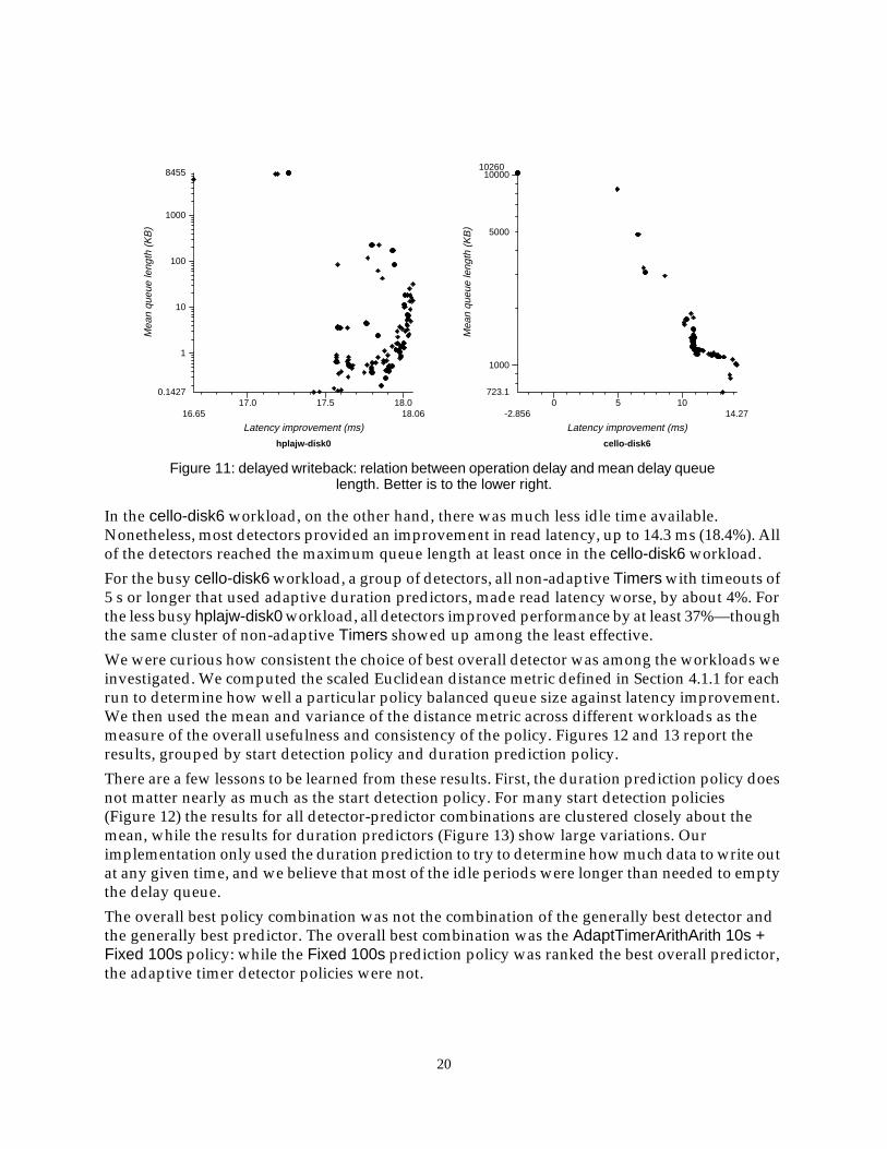
In the cello-disk6 workload, on the other hand, there was much less idle time available.Nonetheless, most detectors provided an improvement in read latency, up to 14.3 ms (18.4%). Allof the detectors reached the maximum queue length at least once in the cello-disk6 workload.

For the busy cello-disk6 workload, a group of detectors, all non-adaptive Timers with timeouts of5 s or longer that used adaptive duration predictors, made read latency worse, by about 4%. Forthe less busy hplajw-disk0 workload, all detectors improved performance by at least 37%—thoughthe same cluster of non-adaptive Timers showed up among the least effective.

We were curious how consistent the choice of best overall detector was among the workloads weinvestigated. We computed the scaled Euclidean distance metric defined in Section 4.1.1 for eachrun to determine how well a particular policy balanced queue size against latency improvement.We then used the mean and variance of the distance metric across different workloads as themeasure of the overall usefulness and consistency of the policy. Figures 12 and 13 report theresults, grouped by start detection policy and duration prediction policy.

There are a few lessons to be learned from these results. First, the duration prediction policy doesnot matter nearly as much as the start detection policy. For many start detection policies(Figure 12) the results for all detector-predictor combinations are clustered closely about themean, while the results for duration predictors (Figure 13) show large variations. Ourimplementation only used the duration prediction to try to determine how much data to write outat any given time, and we believe that most of the idle periods were longer than needed to emptythe delay queue.

The overall best policy combination was not the combination of the generally best detector andthe generally best predictor. The overall best combination was the AdaptTimerArithArith 10s +Fixed 100s policy: while the Fixed 100s prediction policy was ranked the best overall predictor,the adaptive timer detector policies were not.

16.6517.0 17.5 18.0

18.06

Latency improvement (ms)

0.1427

1

10

100

1000

8455

Mea

n qu

eue

leng

th (

KB

)

hplajw-disk0

-2.8560 5 10

14.27

Latency improvement (ms)

723.1

1000

5000

1000010260

Mea

n qu

eue

leng

th (

KB

)

cello-disk6

Figure 11: delayed writeback: relation between operation delay and mean delay queuelength. Better is to the lower right.

20

Overall, however, the rate-based (EventWindow and MovingAverage) start detector policiesshowed less variance than the adaptive timer policies. Our conclusion is that a rate-based policycombined with a simple fixed-duration predictor is a good choice for the write delay idle task.

4.4 Eager LFS segment cleaningOur final idle task was designed to model segment cleaning in a log-structured file system: thesystem must periodically perform garbage-collection operations to compact all the active datatogether [Rosenblum92]. This workload introduces extra housekeeping work into the disksubsystem, beyond the work required for ordinary foreground reads and writes. The goal ofusing idle time is to perform these housekeeping operations at times when there are fewforeground operations. However, the housekeeping has to be performed often enough to avoidrunning out of free space into which new data can be written.

We did not model segment cleaning per se, since we were using traces recorded from systems thatdid not use a log-structured file system. Instead, we constructed an additional workload thatperiodically introduced a burst of read and write traffic similar to a cleaner reading a segment into

0.0 0.5 1.0

Distance from best

PLLTimer 50.0sTimer 10.0sTimer 1.0sTimer 5.0sTimer 0.5s

EventWindow size 100, 0.1 IO/sEventWindow size 250, 0.1 IO/s

AdaptTimerArithGeom 0.100sEventWindow size 250, 1 IO/s

EventWindow size 50, 0.1 IO/sEventWindow size 250, 5 IO/sEventWindow size 100, 5 IO/sEventWindow size 100, 1 IO/sEventWindow size 50, 5 IO/sEventWindow size 50, 1 IO/sAdaptTimerArithArith 0.100sEventWindow size 10, 1 IO/sEventWindow size 10, 5 IO/s

EventWindow size 10, 0.1 IO/sAdaptTimerArithGeom 1.0s

AdaptTimerArithGeom 10.0sMovingAverage 1.0 IO/s

AdaptTimerArithArith 10.0sMovingAverage 10.0 IO/s

EventWindow size 5, 1 IO/sAdaptTimerArithArith 1.0s

EventWindow size 5, 0.1 IO/sMovingAverage 0.1 IO/s

EventWindow size 5, 5 IO/s

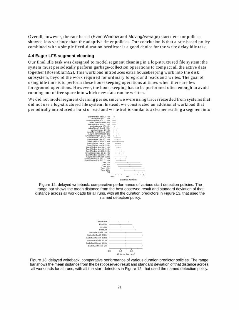
Figure 12: delayed writeback: comparative performance of various start detection policies. Therange bar shows the mean distance from the best observed result and standard deviation of that

distance across all workloads for all runs, with all the duration predictors in Figure 13, that used thenamed detection policy.

0.0 0.2 0.4

Distance from best

BackoffArithGeom 1.0sBackoffArithGeom 0.010s

BackoffArithArith 0.010sBackoffArithGeom 0.100s

BackoffArithArith 0.100sBackoffArithArith 1.0s

Fixed 10sAverage

Fixed 20sFixed 100s

Figure 13: delayed writeback: comparative performance of various duration predictor policies. The rangebar shows the mean distance from the best observed result and standard deviation of that distance acrossall workloads for all runs, with all the start detectors in Figure 12, that used the named detection policy.

21

memory, then writing it out elsewhere. We modeled the amount of data that needed to be copiedby assuming that the file system was in a steady state, so that each byte written created one byteof data that must be copied. While this is not strictly what an LFS cleaner does, we believe that theresulting workload was sufficiently like an LFS cleaner to evaluate idle detector performance.

Specifically, the cleaner task repeatedly executed a cleaning cycle whenever the system was idle.In one cleaning cycle, the task read up to 1MB of data consecutively from one location on the disk,then wrote the data to another location on the disk and advanced the read and write locations forthe next cycle. The cleaner task used the duration prediction from the idleness detection networkto compute how much data could be processed in one cycle without interfering with foregroundwork, and set the amount read in the cycle accordingly. The task would only begin a cycle if itexpected that it could process at least 64KB without interruption. If the cleaner was told by theactuator to stop, it immediately wrote out as much as it had read and then stopped. Interruptionsduring the write portion of the cycle were ignored.

The interference between cleaning and foreground operations was measured by the delayimposed on the foreground operations. This should, of course, be minimized. Most studies on LFSsegment cleaning policies have compared the overall service times using different policies—forexample, comparing background cleaning with cleaning on demand in the foreground[Seltzer93]. For this study, however, we were not modeling an entire log-structured file systemand instead measured interference by the difference in mean service time between the systemwithout cleaning and background cleaning with various idleness detection policies.

Whether housekeeping is being performed often enough was measured by the amount ofunprocessed data. Since we were not modeling garbage collection per se, we instead measuredthe amount of unprocessed data. The lower this amount, the more space was ready to absorb aburst of writes, and hence the less likely it was that a real LFS would have to perform garbagecollection in the foreground.

We report results from the hplajw and cello traces. Since hplajw was lightly used, the amount ofunprocessed data stayed low and the cleaner task had ample opportunity to run. The cello systemwas much busier, so the cleaner had both more work to do and the idle periods were shorter. Wevaried both the start detection and the duration prediction algorithms since this idle task wassensitive to duration predictions.

For both workloads, most idle detectors worked well enough to cause a negligible increase inmean operation delay. For cello-disk6—the busier and thus more difficult system—the worstdetector delayed user operations by an average of 5.2 ms, which was only 1.4% of the originalmean operation service time. (In this trace, many write operations were part of large bursts andthe operation service time included the time spent waiting for preceding operations to complete.)For hplajw-disk0, a lightly used disk, the delay due to the worst detector was slightly less good:6.6 ms, or 6.2% of the original service time.

For the busy cello-disk6 workload, the mean amount of unprocessed data ranged from 3.6 MB to84 MB; a few detectors never declared idleness and thus cause unbounded accumulation. A realLFS would have had to perform foreground cleaning in those cases. For the hplajw-disk0workload, unprocessed data ranged from 0.42 MB to 2.0 MB, with about half the detectorsyielding a mean of less than 0.5 MB. The start detectors that never found idle time were all fixedtimers. Some had too long a timeout value; others used an adaptive duration predictor that didnot receive enough accurate detections to provide usefully-long duration predictions.

22

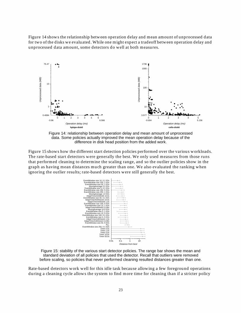
Figure 14 shows the relationship between operation delay and mean amount of unprocessed datafor two of the disks we evaluated. While one might expect a tradeoff between operation delay andunprocessed data amount, some detectors do well at both measures.

Figure 15 shows how the different start detection policies performed over the various workloads.The rate-based start detectors were generally the best. We only used measures from those runsthat performed cleaning to determine the scaling range, and so the outlier policies show in thegraph as having mean distances much greater than one. We also evaluated the ranking whenignoring the outlier results; rate-based detectors were still generally the best.

Rate-based detectors work well for this idle task because allowing a few foreground operationsduring a cleaning cycle allows the system to find more time for cleaning than if a stricter policy

-0.960 1 2 3 4 5 6

6.566

Operation delay (ms)

0.4084

1

10

75.47

Unp

roce

ssed

dat

a (M

B)

hplajw-disk0

-0.0040 1 2 3 4 5

5.156

Operation delay (ms)

3.577

10

100

1000

1736

Unp

roce

ssed

dat

a (M

B)

cello-disk6

Figure 14: relationship between operation delay and mean amount of unprocesseddata. Some policies actually improved the mean operation delay because of the

difference in disk head position from the added work.

0.01 0.1 1 10

Distance from best

Timer 50.0sTimer 10.0sTimer 5.0sTimer 1.0sTimer 0.5s

EventWindow size 250, 0.1 IO/sPLL

EventWindow size 50, 5 IO/sAdaptTimerArithGeom 0.100s

AdaptTimerArithGeom 1.0sEventWindow size 5, 5 IO/s

EventWindow size 100, 0.1 IO/sEventWindow size 10, 5 IO/sEventWindow size 5, 1 IO/s

MovingAverage 10.0 IO/sAdaptTimerArithArith 0.100sEventWindow size 10, 1 IO/s

EventWindow size 100, 5 IO/sAdaptTimerArithArith 1.0s

AdaptTimerArithGeom 10.0sEventWindow size 50, 0.1 IO/s

AdaptTimerArithArith 10.0sMovingAverage 1.0 IO/s

EventWindow size 250, 1 IO/sEventWindow size 250, 5 IO/sEventWindow size 5, 0.1 IO/s

MovingAverage 0.1 IO/sEventWindow size 50, 1 IO/s

EventWindow size 100, 1 IO/sEventWindow size 10, 0.1 IO/s

Figure 15: stability of the various start detector policies. The range bar shows the mean andstandard deviation of all policies that used the detector. Recall that outliers were removed

before scaling, so policies that never performed cleaning resulted distances greater than one.

23

were used—such as a Timer-based policy, which requires absolute idleness in the system. At thesame time, by requiring the IO rate to drop below a fairly low threshold (0.1 or 1 IO/s), the policyensures that few foreground operations will be affected.

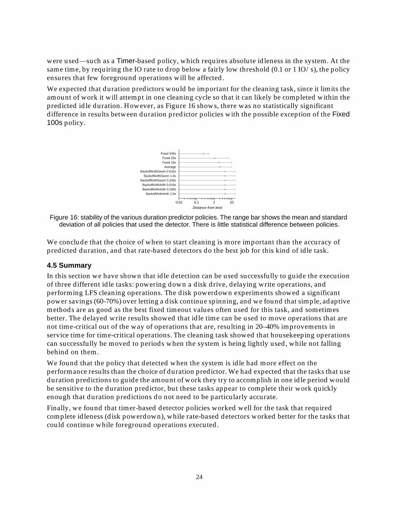
We expected that duration predictors would be important for the cleaning task, since it limits theamount of work it will attempt in one cleaning cycle so that it can likely be completed within thepredicted idle duration. However, as Figure 16 shows, there was no statistically significantdifference in results between duration predictor policies with the possible exception of the Fixed100s policy.

We conclude that the choice of when to start cleaning is more important than the accuracy ofpredicted duration, and that rate-based detectors do the best job for this kind of idle task.

4.5 SummaryIn this section we have shown that idle detection can be used successfully to guide the executionof three different idle tasks: powering down a disk drive, delaying write operations, andperforming LFS cleaning operations. The disk powerdown experiments showed a significantpower savings (60-70%) over letting a disk continue spinning, and we found that simple, adaptivemethods are as good as the best fixed timeout values often used for this task, and sometimesbetter. The delayed write results showed that idle time can be used to move operations that arenot time-critical out of the way of operations that are, resulting in 20–40% improvements inservice time for time-critical operations. The cleaning task showed that housekeeping operationscan successfully be moved to periods when the system is being lightly used, while not fallingbehind on them.

We found that the policy that detected when the system is idle had more effect on theperformance results than the choice of duration predictor. We had expected that the tasks that useduration predictions to guide the amount of work they try to accomplish in one idle period wouldbe sensitive to the duration predictor, but these tasks appear to complete their work quicklyenough that duration predictions do not need to be particularly accurate.

Finally, we found that timer-based detector policies worked well for the task that requiredcomplete idleness (disk powerdown), while rate-based detectors worked better for the tasks thatcould continue while foreground operations executed.

0.01 0.1 1 10

Distance from best

BackoffArithArith 1.0sBackoffArithArith 0.100sBackoffArithArith 0.010s

BackoffArithGeom 0.100sBackoffArithGeom 1.0s

BackoffArithGeom 0.010sAverage

Fixed 10sFixed 20s

Fixed 100s

Figure 16: stability of the various duration predictor policies. The range bar shows the mean and standarddeviation of all policies that used the detector. There is little statistical difference between policies.

24

5 AnalysisThe taxonomic approach we have taken is different from most previous investigations into usingidle time. Most of the policies that the taxonomy describes adapt in some way to system behavior,and most have one or more tuning parameters. In this section we investigate why a taxonomicapproach was beneficial, and why adaptivity was important. We show that performance was notvery sensitive to tuning parameters, suggesting that making a somewhat wrong tuning choice isnot usually catastrophic.

We also investigated how the performance of an idle task using a particular idleness detectionpolicy is related to internal measures of how well that policy can find and predict idle time. Theresults suggest that external performance measures correlate with internal measures only wheneither idle time is difficult to find, as in a busy workload, or when the penalties of an incorrectprediction are high. For other cases, the external performance of the idle tasks is usually very goodand so the choice of policy does not matter so much.

We have one negative result: we investigated whether skeptics (Section 3.2) could improveperformance. The skeptics we investigated did not.

5.1 Effectiveness of the taxonomyTaking a taxonomic approach to analyzing idleness detection was worth the effort. We saw twocosts: the time spent developing the taxonomy, and the computing time spent evaluating the largenumber of detection policies we generated using the taxonomy. The benefits came from thecoverage of the problem space that the taxonomy provided, and the software-engineeringbenefits of a module design guided by the taxonomy.

The cost involved in determining the components was small—a few days discussion among twopeople, spread out over half a month. The implementation effort was also low: one personcompleted the first version of the entire idle processing code except the PLL detectors in abouttwo weeks, including the time spent learning the Pantheon simulator system. The final codeevolved over the next few months, overlapped with other work. The final version of the entiresystem, including the implementation of the three idle tasks, consists of slightly more than 11klines of C++ code and 600 lines of Tcl code.

As a benefit, the taxonomy adequately covers the kinds of idleness detection we have seen usedin practice. We have been pleased to find that all of the work that we are aware of that has beenpublished since our first paper [Golding95] has fallen neatly into this taxonomic structure. Forexample, Douglis et al. [1995], while developing adaptive disk power-down policies, investigatedthe use of adaptive timers with either arithmetic or geometric adjustment. The primarydifferences between their policies and our AdaptTimer policies are that they considered usingdifferent increment values for increase and decrease; they limit the smallest and largest timervalues; and the decision to adjust the timer depends on an application-specific condition (whetherrecent spindown activity has met a user goal or not). Likewise, Helmbold et al. [Helmbold96]have investigated using a skeptic based on machine learning techniques to choose the best fromamong a family of fixed timer detectors. In both these examples, we found that having ataxonomy helps identify the essential characteristics of their work, separate from the specificproblem that they were investigating, and suggest ways that the ideas can be generalized or usedfor other problems.

Dividing the problem into smaller components made implementation easier. The usual softwareengineering arguments for modularity applied to this problem: the individual start detection,

25

duration prediction, and skeptic objects are quite simple, often consisting of less than twenty linesof non-boilerplate code. Being able to combine different policies at runtime meant we couldinvestigate a large policy space with a small implementation effort.

Using a taxonomic approach helped us to find better policies than we might otherwise havefound. Consider how different the ranking of idleness detection policies is among the threesample idle tasks. If we had considered only, say, the adaptive timer detectors—which are bestfor disk powerdown and delayed writeback—we would not have found any of the overall bestdetectors for segment cleaning, which are all rate-based. Moreover, the absolute best idlenessdetection policy combination for delayed writeback across all the workloads did not use the bestoverall detector start detection policy, which indicates that it was necessary to look at all the startdetector/duration predictor combinations.

The taxonomy also generated some surprises. For example, we had previously believed that theEventWindow detectors would work better with long windows, in order to remove the effects oftransient burst behavior. The measured results differed from our expectations, and on furtherinvestigation we found that a long window did not allow the detector to react quickly enoughwhen the system stopped being idle.

5.2 The importance of adaptationMany of the idleness detection and prediction policies we have investigated try to adapt to thesystem they monitor. Such adaptation has two purposes: it reduces the sensitivity of an initialdesign to later deployments, and it allows a running system to adapt to changing requirements.

To illustrate the importance of adaptation, we performed a simple analysis on our traces.Consider a system where the “benefit” b of using an idle period of duration d is quantifiable as

, which is a simplification of the energy savings in Joules from the disk power-downidle task. If a fixed timeout policy of length t is used to detect the start of an idle period, then theoverall benefit becomes . We performed an offline analysis to find the timeoutperiod that maximized this benefit, using traces from four systems: the three systems we used forevaluating idle tasks in Section 4, plus a one-hour trace of a very busy transaction-processingsystem. We considered both the timeout value that maximized the benefit over each entire trace(the trace-optimal timeout), and the optimum values for each hour subset of the traces (the hourly-optimal timeout).

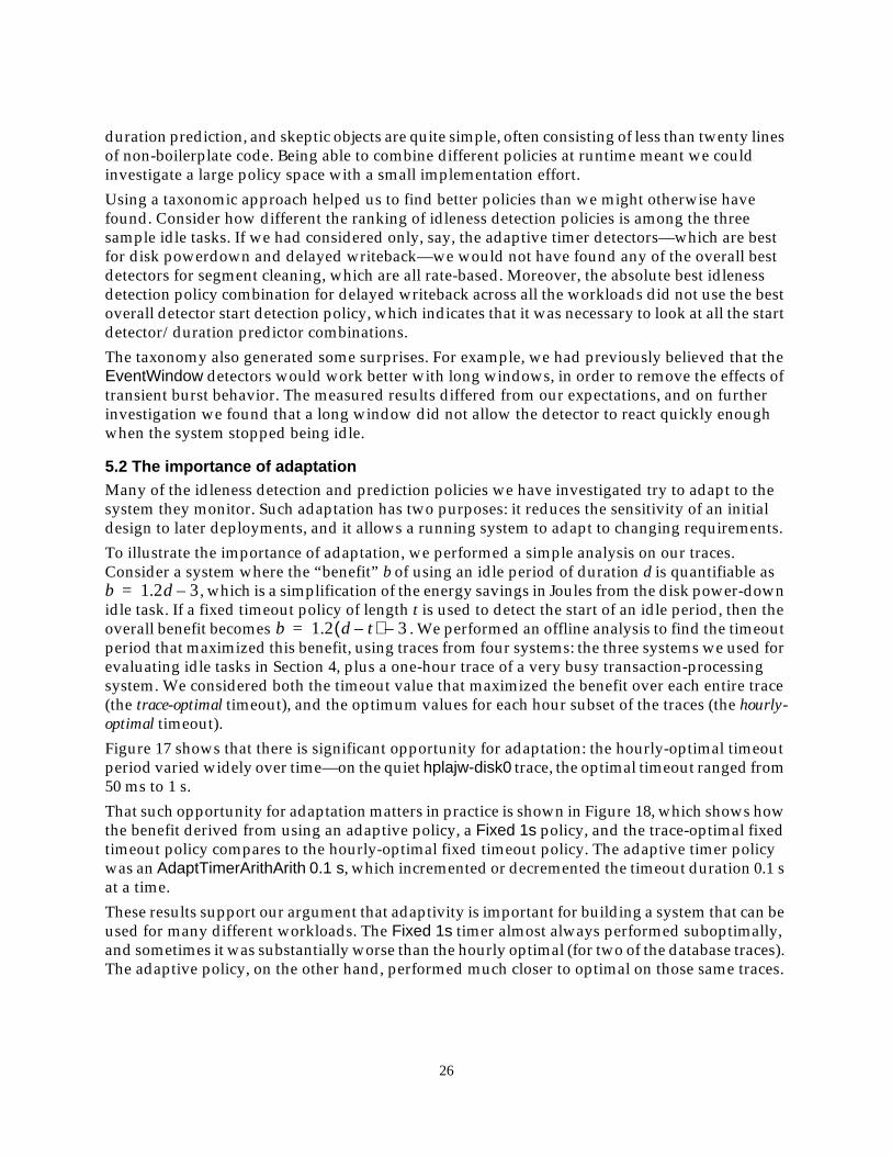
Figure 17 shows that there is significant opportunity for adaptation: the hourly-optimal timeoutperiod varied widely over time—on the quiet hplajw-disk0 trace, the optimal timeout ranged from50 ms to 1 s.

That such opportunity for adaptation matters in practice is shown in Figure 18, which shows howthe benefit derived from using an adaptive policy, a Fixed 1s policy, and the trace-optimal fixedtimeout policy compares to the hourly-optimal fixed timeout policy. The adaptive timer policywas an AdaptTimerArithArith 0.1 s, which incremented or decremented the timeout duration 0.1 sat a time.

These results support our argument that adaptivity is important for building a system that can beused for many different workloads. The Fixed 1s timer almost always performed suboptimally,and sometimes it was substantially worse than the hourly optimal (for two of the database traces).The adaptive policy, on the other hand, performed much closer to optimal on those same traces.

b 1.2d 3–=

b 1.2 d t–( ) 3–=

26

Adaptivity is also useful in tracking short-term changes within a workload, and an hourlygranularity is too coarse. The adaptive policy almost always did as well or better than the hourly-optimal fixed timeout policy, which in turn did better than the trace-optimal fixed timeout.

When we changed the benefit formula so that the break-even point was much longer than in ourprevious formula, , the differences become more pronounced, as shown inthe lower graph in Figure 18. While the Fixed 1 s timer policy sometimes got equal or higherbenefit than the adaptive timer, the adaptive timer was more consistent. In two of the databasetraces, the best benefit came from never using idle time. These bars are omitted from the graph.

Our conclusion is that adaptivity helps to make idleness detection resilient to differences inworkloads and to changing workloads, in many cases yielding results close to optimal.

5.3 Relations between internal and external measuresWhen building a system, one would like to find a good idleness detector without performing theexhaustive evaluation we did for our three example idle tasks. Ideally, one could make aprediction of which detectors will work well based on their internal measures when measuredagainst a similar workload.

In the following sections we will first define a number of internal measures, then look at how theexternal measures for our example idle tasks were related to them. The results from ourinvestigation are mixed: we found correlation between internal and external measures for someof our applications, but not for others.

5.3.1 Internal performance measuresInternal measures quantify how well a particular detector finds idle periods, and are independentof a particular idle task.

Taking the internal measurements depends on an application-specified level of acceptableidleness. The simplest definition was that the system should be considered idle whenever therewere no requests active. We used this definition because it is trivial to detect on-line. A more

hplajw-disk0

00 50 100 150

167

Time (hours)

0 0.00.0

0.5

1

Opt

imal

tim

eout

(se

cond

s)

hplajw-disk0

hourlyoverall

cello-disk6

00 50 100 150

167

Time (hours)

0 00

1

2

2.25

Opt

imal

tim

eout

(se

cond

s)

cello-disk6

hourlyoverall

Figure 17: optimal fixed timeout values for two traces.

b 1.2 d t–( ) 15–=

27

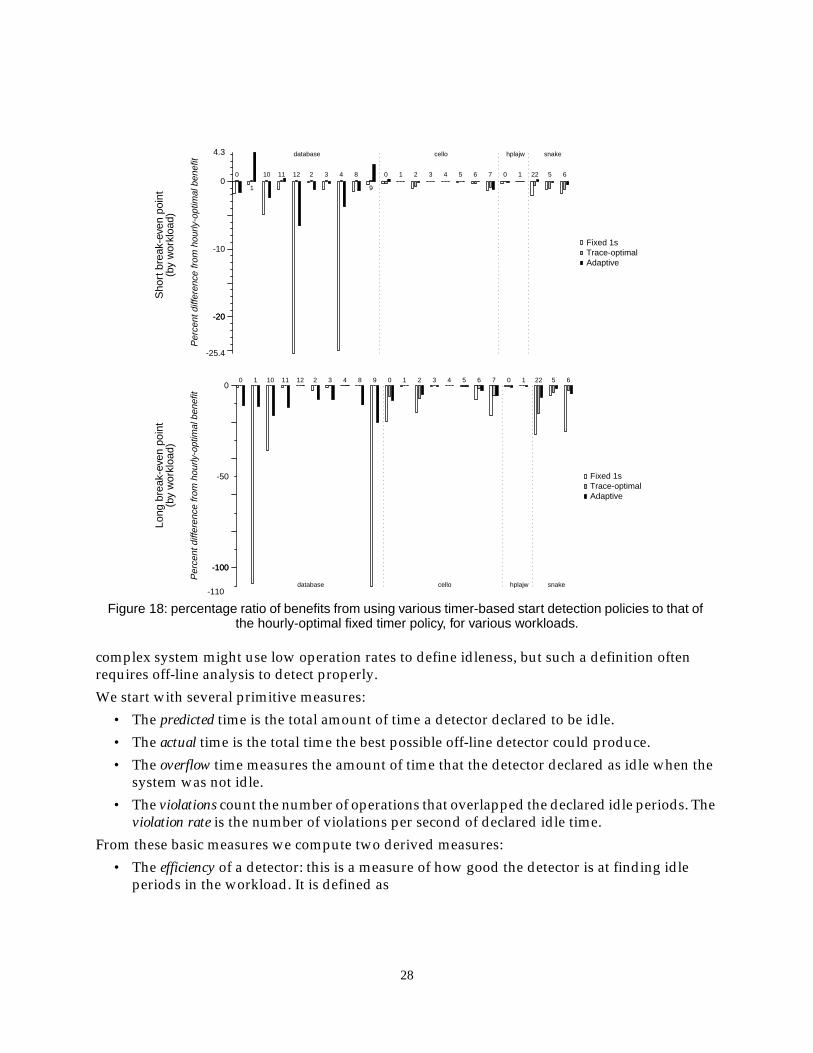
complex system might use low operation rates to define idleness, but such a definition oftenrequires off-line analysis to detect properly.

We start with several primitive measures:

• The predicted time is the total amount of time a detector declared to be idle.

• The actual time is the total time the best possible off-line detector could produce.

• The overflow time measures the amount of time that the detector declared as idle when thesystem was not idle.

• The violations count the number of operations that overlapped the declared idle periods. Theviolation rate is the number of violations per second of declared idle time.

From these basic measures we compute two derived measures:

• The efficiency of a detector: this is a measure of how good the detector is at finding idleperiods in the workload. It is defined as

-25.4

-20-20

-10

0

4.3

Per

cent

diff

eren

ce fr

om h

ourly

-opt

imal

ben

efit

Fixed 1sTrace-optimalAdaptive

database snakehplajwcello

0

1

10 11 12 2 3 4 8

9

0 1 2 3 4 5 6 7 0 1 22 5 6

-110

-100-100

-50

0

Per

cent

diff

eren

ce fr

om h

ourly

-opt

imal

ben

efit

Fixed 1sTrace-optimalAdaptive

database snakehplajwcello

0 1 10 11 12 2 3 4 8 9 0 1 2 3 4 5 6 7 0 1 22 5 6

Figure 18: percentage ratio of benefits from using various timer-based start detection policies to that ofthe hourly-optimal fixed timer policy, for various workloads.

Sho

rt b

reak

-eve

n po

int

(by

wor

kloa

d)Lo

ng b

reak

-eve

n po

int

(by

wor

kloa

d)

28

efficiency = (predicted - overflow) / actualThat is, it is the fraction of actual idle time that was declared idle.

• A detector’s incompetence evaluates how much of the predicted idle time is not idle,penalizing over-eager detectors. It is defined as

incompetence = overflow / actualA good idleness detector will have a high efficiency and a low incompetence.

5.3.2 RelationsWe investigated the relationship between internal and external measures by measuring theefficiency and violation rate produced by each idleness detection policy, then determiningwhether the results for that policy correlated with the external performance measures for thethree different idle tasks.Table 6 summarizes the results. We measured the relationships betweenmeasures by looking for correlation at a 95% confidence level.

• Disk power-down: we found close correlations between the two external measures—powersavings and the number of delayed operations—and both efficiency and violation rate.There was one exception: the PLL detectors simply did the wrong thing most of the time.Efficiency is correlated with power savings because an efficient detector is finding most ofthe opportunities to have the disk powered down. Violation rate is correlated with powersavings because the length of time spent powered down in any one idle period wasdetermined by the time until the next operation arrives, which is on average the inverse ofthe violation rate.

Table 6: relations between internal and external performance measures.

External measure Efficiency Violation rate

Powerdown:

Energy yes yes, except forPLL detectors

Operation delay yes, except forPLL detectors yes

Delayed writeback:

Mean queue length yes no

Latency improvementyes

(only busyworkloads)

no

Distance metricyes

(only busyworkloads)

no

LFS segment cleaning:

Mean unprocessed data yes no

Operation delay yes no

Distance metricyes, except for

some Fixedtimers

no

29

• Delayed writeback: the violation rate does not appear to be related to any of the externalmeasures we took. Delayed writeback is relatively insensitive to occasional overlappedforeground and background operations. We could not establish correlations with efficiencyfor the traces from quiet disks, because nearly all idleness detection policies yieldedefficiency greater than 90%. For the busy cello-disk6 workload, however, efficiency clearlycorrelated with all three external measures. This is because an efficient idleness detectionpolicy will find more time to flush the delay queue than an inefficient detection policy.

• Eager LFS segment cleaning: once again, the violation rate was not related to the externalmeasures because it was rare for a cleaning cycle to run long enough be interrupted by newwork arriving—for most idleness detection policies, less than 5% of cleaning cycles for thebusy cello-disk6 workload, and much lower for quiet disks. Efficiency, on the other hand,was correlated with all three external measures, with the exception noted in Section 4.4 of agroup of fixed Timer detectors that did especially poorly.

These results suggest that internal measures are correlated with external one only when there islittle idle time available or when the penalty of getting a poor prediction is high. Our conclusionis that internal measures may be helpful in finding a good detector for heavily-loaded orpathological situations, but that most of the time the problems are undemanding, the results areuniformly good and hence there is little guidance to be had from the internal measures.

5.4 Sensitivity of internal measures to policy parametersMost families of idle detection mechanisms in our taxonomy can be tuned to provide differentbehaviors. We investigated two example policies—one start detector and one durationpredictor—to determine how sensitive their internal performance measures are to their tuningparameters. We found that they were generally well behaved: while there usually is an optimumparameter setting, the results from nearby settings were not much worse. We also found that theresults, when they matter, are similar between busy and quiet workloads.

5.4.1 Start detection policy parametersWe investigated tuning the EventWindow+IO rate threshold detector because its externalperformance varied depending on its parameter settings. For example, at low rate thresholds thedetector yielded good power savings for disk powerdown, but high rate thresholds did poorly.

The detector is parameterized by rate threshold and window size. The rate threshold governshow quiet the system must be before being declared idle. We expected a low threshold to give lowefficiency, because it would take some time for the mean IO rate to drop below the threshold, andthe waiting period could have been used profitably. A low threshold should, however, give a lowviolation rate. The window size governs responsiveness: a small window means the detectorreacts quickly to changes, but it may prematurely declare idleness. A large window may cause thedetector react too slowly to start of idleness and to the start of a burst of requests.

To measure the effects of tuning a detector, we set up an experiment to take internal measureswith a no-op idle task and a Fixed 10 s duration predictor. The actuator was parameterized tofollow the predictions exactly: when it received a prediction, the idle task ran for 10 s, whethernew work arrived or not. We took measurements from a quiet disk (hplajw-disk0) and a busy one(cello-disk6).

On the quiet disk, the violation rate was relatively insensitive to the window size. Bursts ofrequests were small and infrequent, so there was plenty of time for the average rate to drop below

30

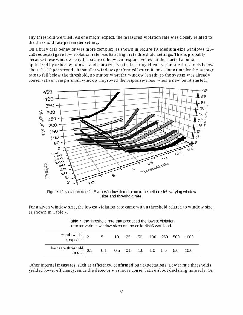
any threshold we tried. As one might expect, the measured violation rate was closely related tothe threshold rate parameter setting.

On a busy disk behavior was more complex, as shown in Figure 19. Medium-size windows (25–250 requests) gave low violation rate results at high rate threshold settings. This is probablybecause these window lengths balanced between responsiveness at the start of a burst—optimized by a short window—and conservatism in declaring idleness. For rate thresholds belowabout 0.1 IO per second, the smaller windows performed better. It took a long time for the averagerate to fall below the threshold, no matter what the window length, so the system was alreadyconservative; using a small window improved the responsiveness when a new burst started.

For a given window size, the lowest violation rate came with a threshold related to window size,as shown in Table 7.

Other internal measures, such as efficiency, confirmed our expectations. Lower rate thresholdsyielded lower efficiency, since the detector was more conservative about declaring time idle. On

Table 7: the threshold rate that produced the lowest violationrate for various window sizes on the cello-disk6 workload.

window size(requests) 2 5 10 25 50 100 250 500 1000

best rate threshold(IO/s) 0.1 0.1 0.5 0.5 1.0 1.0 5.0 5.0 10.0

450

400

350

300

250

200

150

100

50

0

Vio

latio

n ra

te

Violation rateWindow size

Threshold rate

050

100150200250300350400450

25

102550

1002505001000

0.010.05

0.1

0.5

1

5

10

Figure 19: violation rate for EventWindow detector on trace cello-disk6, varying windowsize and threshold rate.

31

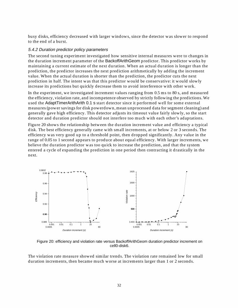
busy disks, efficiency decreased with larger windows, since the detector was slower to respondto the end of a burst.

5.4.2 Duration predictor policy parametersThe second tuning experiment investigated how sensitive internal measures were to changes inthe duration increment parameter of the BackoffArithGeom predictor. This predictor works bymaintaining a current estimate of the next duration. When an actual duration is longer than theprediction, the predictor increases the next prediction arithmetically by adding the incrementvalue. When the actual duration is shorter than the prediction, the predictor cuts the nextprediction in half. The intent was that this predictor would be conservative: it would slowlyincrease its predictions but quickly decrease them to avoid interference with other work.

In the experiment, we investigated increment values ranging from 0.5 ms to 80 s, and measuredthe efficiency, violation rate, and incompetence observed by strictly following the predictions. Weused the AdaptTimerArithArith 0.1 s start detector since it performed well for some externalmeasures (power savings for disk powerdown, mean unprocessed data for segment cleaning) andgenerally gave high efficiency. This detector adjusts its timeout value fairly slowly, so the startdetector and duration predictor should not interfere too much with each other’s adaptations.

Figure 20 shows the relationship between the duration increment value and efficiency a typicaldisk. The best efficiency generally came with small increments, at or below 2 or 3 seconds. Theefficiency was very good up to a threshold point, then dropped significantly. Any value in therange of 0.05 to 1 second appears to produce about equal efficiency. With larger increments, webelieve the duration predictor was too quick to increase the prediction, and that the systementered a cycle of expanding the prediction in one period then contracting it drastically in thenext.

The violation rate measure showed similar trends. The violation rate remained low for smallduration increments, then became much worse at increments larger than 1 or 2 seconds.

0.00050.001 0.01 0.1 1 10

80

Duration increment (s)

0.885

0.900.90

0.92

0.94

0.96

0.980.9832

Effi

cien

cy

0.00050.001 0.01 0.1 1 10

80

Duration increment (s)

3.403

500500

1000

1500

1925

Vio

latio

n ra

te

Figure 20: efficiency and violation rate versus BackoffArithGeom duration predictor increment oncell0-disk6.

32

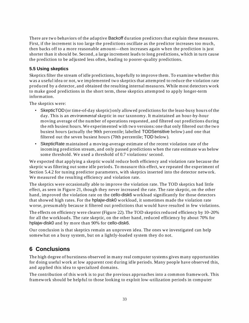
There are two behaviors of the adaptive Backoff duration predictors that explain these measures.First, if the increment is too large the predictions oscillate as the predictor increases too much,then backs off to a more reasonable amount—then increases again when the prediction is justshorter than it should be. Second, a large increment leads to long predictions, which in turn causethe prediction to be adjusted less often, leading to poorer-quality predictions.

5.5 Using skepticsSkeptics filter the stream of idle predictions, hopefully to improve them. To examine whether thiswas a useful idea or not, we implemented two skeptics that attempted to reduce the violation rateproduced by a detector, and obtained the resulting internal measures. While most detectors workto make good predictions in the short term, these skeptics attempted to apply longer-terminformation.

The skeptics were:

• SkepticTOD (or time-of-day skeptic) only allowed predictions for the least-busy hours of theday. This is an environmental skeptic in our taxonomy. It maintained an hour-by-hourmoving average of the number of operations requested, and filtered out predictions duringthe nth busiest hours. We experimented with two versions: one that only filtered out the twobusiest hours (actually the 90th percentile; labelled TODSensitive below) and one thatfiltered out the seven busiest hours (70th percentile; TOD below).

• SkepticRate maintained a moving-average estimate of the recent violation rate of theincoming prediction stream, and only passed predictions when the rate estimate was belowsome threshold. We used a threshold of 0.7 violations/second.

We expected that applying a skeptic would reduce both efficiency and violation rate because theskeptic was filtering out some idle periods. To measure this effect, we repeated the experiment ofSection 5.4.2 for tuning predictor parameters, with skeptics inserted into the detector network.We measured the resulting efficiency and violation rate.

The skeptics were occasionally able to improve the violation rate. The TOD skeptics had littleeffect, as seen in Figure 21, though they never increased the rate. The rate skeptic, on the otherhand, improved the violation rate on the cello-disk6 workload significantly for those detectorsthat showed high rates. For the hplajw-disk0 workload, it sometimes made the violation rateworse, presumably because it filtered out predictions that would have resulted in few violations.

The effects on efficiency were clearer (Figure 22). The TOD skeptics reduced efficiency by 10–20%for all the workloads. The rate skeptic, on the other hand, reduced efficiency by about 70% forhplajw-disk0 and by more than 90% for cello-disk6.

Our conclusion is that skeptics remain an unproven idea. The ones we investigated can helpsomewhat on a busy system, but on a lightly-loaded system they do not.

6 ConclusionsThe high degree of burstiness observed in many real computer systems gives many opportunitiesfor doing useful work at low apparent cost during idle periods. Many people have observed this,and applied this idea to specialized domains.

The contribution of this work is to put the previous approaches into a common framework. Thisframework should be helpful to those looking to exploit low-utilization periods in computer

33

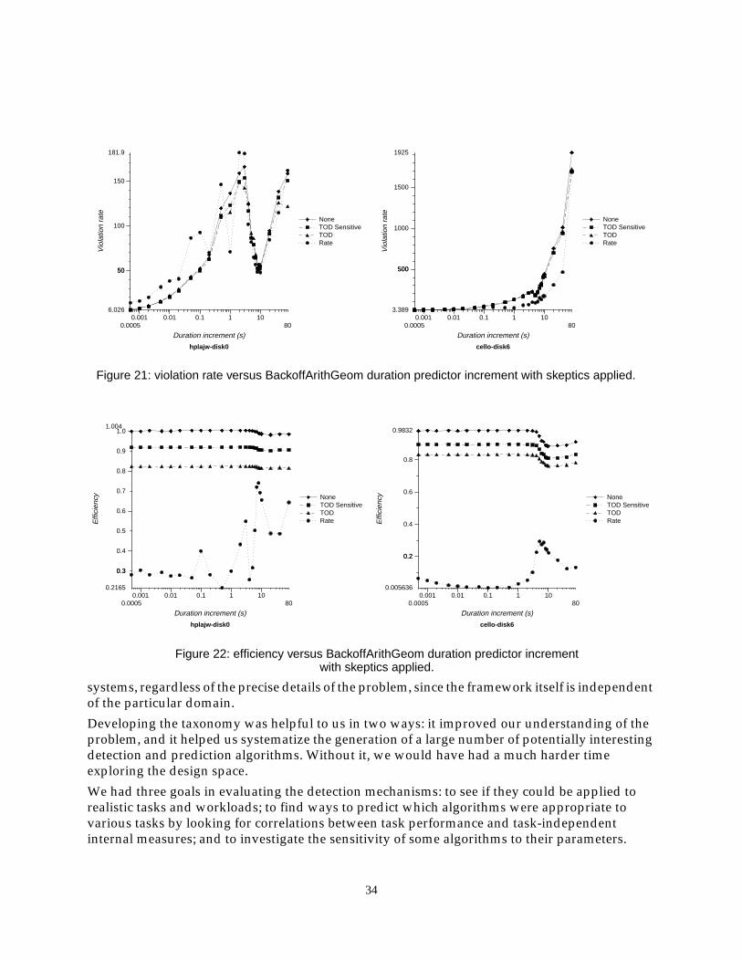
systems, regardless of the precise details of the problem, since the framework itself is independentof the particular domain.

Developing the taxonomy was helpful to us in two ways: it improved our understanding of theproblem, and it helped us systematize the generation of a large number of potentially interestingdetection and prediction algorithms. Without it, we would have had a much harder timeexploring the design space.

We had three goals in evaluating the detection mechanisms: to see if they could be applied torealistic tasks and workloads; to find ways to predict which algorithms were appropriate tovarious tasks by looking for correlations between task performance and task-independentinternal measures; and to investigate the sensitivity of some algorithms to their parameters.

0.00050.001 0.01 0.1 1 10

80

Duration increment (s)

6.026

5050

100

150

181.9

Vio

latio

n ra

te

hplajw-disk0

NoneTOD SensitiveTODRate

0.00050.001 0.01 0.1 1 10

80

Duration increment (s)

3.389

500500

1000

1500

1925

Vio

latio

n ra

te

cello-disk6

NoneTOD SensitiveTODRate

Figure 21: violation rate versus BackoffArithGeom duration predictor increment with skeptics applied.

0.00050.001 0.01 0.1 1 10

80

Duration increment (s)

0.2165

0.30.3

0.4

0.5

0.6

0.7

0.8

0.9

1.01.004

Effi

cien

cy

hplajw-disk0

NoneTOD SensitiveTODRate

0.00050.001 0.01 0.1 1 10

80

Duration increment (s)

0.005636

0.20.2

0.4

0.6

0.8

0.9832

Effi

cien

cy

cello-disk6

NoneTOD SensitiveTODRate

Figure 22: efficiency versus BackoffArithGeom duration predictor incrementwith skeptics applied.

34

We were gratified to learn that simple predictors work remarkably well at our idle tasks. This isgood news: it means that these techniques can be applied successfully in the real world with onlymoderate effort. Rate-based detectors, in particular, work well for idle tasks that can beoverlapped with while regular work.

Some detectors and predictors were quite sensitive to their parameters. The quickness with whichan EventWindow detector reacted, for example, depended both on the threshold rate and windowsize.

The self-adapting nature of some of the idleness detectors proved useful, and the adaptivealgorithms were often among the best. For some algorithms, the best parameterization valuesdepended on the workload—which could change over time. Rather than have users manuallyestimate the best value, adaptive mechanisms can automatically adjust to the workload.

The external measures specific to the idle tasks were sometimes related to basic internal measures.For most of the tasks we started with suspicions about how the idle detectors should behave toproduce a good result; for example, we were pretty sure that efficiency was important for savingpower in the disk spindown task. For the segment cleaning task, on the other hand, while weexpected that a low violation rate was important, we did not have intuition about the tradeoffbetween finding short idle periods often versus long periods more rarely. We discussed the actualrelations in Section 5.3.

The implementation of idleness detectors proved straightforward, though we learned a fewlessons along the way. We learned that we needed to be sure that adaptive algorithms were ableto update their state often to react quickly to changes. We discovered that the notion of continuinga prediction (Section 3.1.3) was useful.

If the foreground work is similar to the storage system traces we used, we can make some generalrecommendations for picking the best detectors for a task:

• if the idle task completely blocks regular work, or if the cost of interrupting the task is high,then a low violation rate is important. Various kinds of Timer and AdaptTimer detectorswork well for this, though the adaptive versions may be more resilient to a wide range ofworkloads.

• if regular work can continue while the idle task is executing, albeit with some interference,then rate-based detectors, such as the EventWindow and MovingAverage policies, are oftena good choice.

• if the granularity of the idle task is large, or the cost of using an inaccurate prediction is high,then prediction duration is important. The adaptive BackoffArithArith andBackoffArithGeom predictors, using a duration increment parameter in the range 0.1 to 1.0 s,often work well.

• the selection of the absolute best tuning parameters isn’t usually important, becauseperformance often appears to be stable within a range of parameter values.

6.1 Future directionsWe limited our investigation to simple policies, so there are many additions that could be madeto this work. Idleness detection is closely related to the general problem of predicting futureevents, given a series of recent past events. More sophisticated time series analytic approachescould be used for this purpose. There are machine learning techniques that could potentially doeven better. We also have wondered about, but did not investigate, the effect of having policies

35

use application-specific feedback, such as how much housekeeping got done during onepredicted period.

Our investigation of skeptics was at best cursory, and could easily be extended.

AcknowledgmentsGeorge Neville-Neil suggested predictors based on the first derivative of arrival rate, and readseveral early drafts of this work. Fred Douglis’s interest in disk power conservation spurred muchof our early thinking. Darrell Long and David Helmbold, at U. C. Santa Cruz, suggested thepossibility of using machine learning techniques. The feedback from reviewers and readers of ourearlier paper on this subject helped to clarify our thinking and analysis. The other members of theStorage Systems Program at Hewlett-Packard Labs have provided support, encouragement, andcomments all during this project.

References[Baker92b] Mary Baker, Satoshi Asami, Etienne Deprit, John Ousterhout, and Margo Seltzer. Non-

volatile memory for fast, reliable file systems. Proceedings of 5th International Conference onArchitectural Support for Programming Languages and Operating Systems (Boston, MA, 12–15October 1992). Published as Computer Architecture News, 20(special issue):10–22, October 1992.

[Bosch94] Peter Bosch. A cache odyssey. M.Sc. thesis, published as Technical Report SPA–94–10.Faculty of Computer Science/SPA, Universiteit Twente, Netherlands, 23 June 1994.

[Box94] George E. P. Box, Gwilym M. Jenkins, and Gregory C. Reinsel. Time series analysis:forecasting and control, third edition. Prentice-Hall, Englewood Cliffs, NJ, 1994.

[Bubenik89] Rick Bubenik and Willy Zwaenepoel. Performance of optimistic make. Proceedings of1989 ACM SIGMETRICS and Performance ’89 International Conference on Measurement andModeling of Computer Systems (Berkeley, CA). Published as Performance Evaluation Review,17(1):39–48, May 1989.

[Cáceres93] Ramón Cáceres, Fred Douglis, Kai Li, and Brian Marsh. Operating system implicationsof solid-state mobile computers. Technical report MITL–TR–56–93. Matsushita InformationTechnology Laboratory, Princeton, NJ, May 1993.

[Carson92a] Scott Carson and Sanjeev Setia. Optimal write batch size in log-structured filesystems. USENIX Workshop on File Systems (Ann Arbor, MI), pages 79–91, 21–22 May 1992.

[CesaBianchi94] N. Cesa-Bianchi, Y. Freund, D. P. Helmbold, and M. Warmuth. On-line predictionand conversion strategies. Technical report UCSC–CRL–94–28. Computer and InformationSciences Board, University of California at Santa Cruz, August 1994.

[Chen96b] Peter M. Chen. Optimizing delay in delayed-write file systems. Technical report CSE–TR–293–96. University Michigan, May 1996.

[Comer91] Douglas E. Comer and David L. Stevens. Internetworking with TCP/IP: design,implementation, and internals, volume II. Prentice-Hall, 1991.

[Cruz92] Rene L. Cruz. Service burstiness and dynamic burstiness measures: a framework.Journal of High Speed Networks, 2:105–27. IOS press, Amsterdam, 1992.

[Douglis95] Fred Douglis, P. Krishnan, and Brian Bershad. Adaptive disk spin-down policies formobile computers. Proceedings of Second Usenix Symposium on Mobile and Location-IndependentComputing (Ann Arbor, MI). Usenix Association, 10–11 April 1995.

36

[Ganger94b] Gregory R. Ganger and Yale N. Patt. Metadata update performance in file systems.Proceedings of 1st OSDI. (Monterey, CA), pages 49–60. Usenix Association, 14–17 November1994.

[Golding95] Richard Golding, Peter Bosch, Carl Staelin, Tim Sullivan, and John Wilkes. Idlenessis not sloth. Proceedings of Winter USENIX 1995 Technical Conference (New Orleans, LA), pages201–12. Usenix Association, Berkeley, CA, 16–20 January 1995.

[Greenawalt94] Paul M. Greenawalt. Modeling power management for hard disks. 2ndInternational Workshop on Modeling, Analysis and Simulation of Computer and TelecommunicationsSystems (MASCOTS ’94) (Durham, NC), pages 62–6. IEEE Computer Society Press, LosAlamitos, CA, 31 January–2 February 1994.

[Gribble96] Steven D. Gribble, Gurmeet Singh Manku, and Eric A. Brewer. Self-similarity in filesystems: measurement and applications, 1996. Available athttp://www.cs.berkeley.edu/ gribble/cs262/project/project.html.

[Helmbold96] David P. Helmbold, Darrell D. E. Long, and Bruce Sherrod. A dynamic disk spin-down technique for mobile computing. Proceedings of 2nd Annual International Conference onMobile Computing and Networking (MOBICOM) (Rye, NY), 10–12 November 1996.

[HPKittyhawk92] Hewlett-Packard Company, Boise, Idaho. HP Kittyhawk Personal StorageModule: product brief, Part number 5091–4760E, 1992.

[Jacobson91] David M. Jacobson and John Wilkes. Disk scheduling algorithms based on rotationalposition. Technical report HPL–CSP–91–7. Hewlett-Packard Laboratories, 24 February 1991,revised 1 March 1991.

[Karn91] Phil Karn and Craig Partridge. Improving round-trip time estimates in reliable transportprotocols. ACM Transactions on Computer Systems, 9(4):364–73, November 1991.

[Lindsey81] William C. Lindsey and Chak Ming Chie. A survey of digital phase-locked loops. InWilliam C. Lindsey, editor, Phase Locked Loops, pages 296–317. Institute of Electrical andElectronics Engineers, April 1981.

[Marsh93] Brian Marsh, Fred Douglis, and P. Krishnan. Flash memory file caching for mobilecomputers. Technical report MITL–TR–59–93. Matsushita Information Technology Laboratory,Princeton, NJ, 18 June 1993.

[Massalin89a] Henry Massalin and Calton Pu. Fine-grain scheduling. Proceedings of Workshop onExperience in Building Distributed and Multiprocessor Systems (Ft. Lauderdale, FL), pages 91–104.USENIX Association, October 1989.

[Postel80a] J. Postel. Transmission Control Protocol, Technical report RFC–761. USC InformationSciences Institute, January 1980.

[Rodeheffer91] Thomas L. Rodeheffer and Michael D. Schroeder. Automatic reconfiguration inAutonet. Proceedings of 13th ACM Symposium on Operating Systems Principles (Asilomar, PacificGrove, CA). Published as Operating Systems Review, 25(5):183–97, 13–16 October 1991.

[Rosenblum92] Mendel Rosenblum and John K. Ousterhout. The design and implementation of alog-structured file system. ACM Transactions on Computer Systems, 10(1):26–52, February 1992.

[Ruemmler93] Chris Ruemmler and John Wilkes. UNIX disk access patterns. Proceedings of Winter1993 USENIX (San Diego, CA), pages 405–20, 25–29 January 1993.

[Ruemmler94] Chris Ruemmler and John Wilkes. An introduction to disk drive modeling. IEEEComputer, 27(3):17–28, March 1994.

37

[Seltzer90b] Margo Seltzer, Peter Chen, and John Ousterhout. Disk scheduling revisited.Proceedings of Winter 1990 USENIX Conference (Washington, D.C.), pages 313–23, 22–26January 1990.

[Seltzer93] Margo Seltzer, Keith Bostic, Marshall Kirk McKusick, and Carl Staelin. Animplementation of a log-structured file system for UNIX. Proceedings of Winter 1993 USENIX(San Diego, CA, 25–29 January 1993), pages 307–26, January 1993.

[Wilkes92b] John Wilkes. Predictive power conservation. Technical report HPL–CSP–92–5.Concurrent Systems Project, Hewlett-Packard Laboratories, 14 February 1992.

[Wilkes95] John Wilkes. The Pantheon storage-system simulator. Technical Report HPL–SSP–95–14.Storage Systems Program, Hewlett-Packard Laboratories, Palo Alto, CA, 29 December 1995.

38