Deutsches Institut für Wirtschaftsforschung

www.diw.de

Frank M. Fossen • Daniela Glocker

Berlin, October 2009

Expected Future Earnings, Taxation, and University Enrollment: A Microeconometric Model with Uncertainty

934

Discussion Papers

Opinions expressed in this paper are those of the author and do not necessarily reflect views of the institute. IMPRESSUM © DIW Berlin, 2009 DIW Berlin German Institute for Economic Research Mohrenstr. 58 10117 Berlin Tel. +49 (30) 897 89-0 Fax +49 (30) 897 89-200 http://www.diw.de ISSN print edition 1433-0210 ISSN electronic edition 1619-4535 Available for free downloading from the DIW Berlin website. Discussion Papers of DIW Berlin are indexed in RePEc and SSRN. Papers can be downloaded free of charge from the following websites: http://www.diw.de/english/products/publications/discussion_papers/27539.html http://ideas.repec.org/s/diw/diwwpp.html http://papers.ssrn.com/sol3/JELJOUR_Results.cfm?form_name=journalbrowse&journal_id=1079991

Expected Future Earnings, Taxation, and University

Enrollment: A Microeconometric Model with

Uncertainty∗

Frank M. Fossen† Daniela Glocker‡

DIW Berlin

October 2009

Abstract

Taxation changes the expectations of prospective university students about theirfuture level and uncertainty of after-tax income. To estimate the impact of taxeson university enrollment, we develop and estimate a structural microeconometricmodel, in which a high-school graduate decides to enter university studies if expectedlifetime utility from this choice is greater than that anticipated from starting to workright away. We estimate the ex-ante future paths of the expectation and variance ofnet income for German high-school graduates, using only information available tothose graduates at the time of the enrollment decision, accounting for multiple non-random selection and employing a microsimulation model to account for taxation. Inaddition to income uncertainty, the enrollment model takes into account universitydropout and unemployment risks, as well as potential credit constraints. The esti-mation results are consistent with expectations. First, higher risk-adjusted returnsto an academic education increase the probability of university enrollment. Second,high-school graduates are moderately risk averse, as indicated by the Arrow-Prattcoefficient of risk aversion estimated within the model. Thus, higher uncertaintyamong academics decreases enrollment rates. A simulation based on the estimatedstructural model indicates that a revenue-neutral, flat-rate tax reform with an un-changed basic tax allowance would increase enrollment rates for men in Germanybecause of the higher expected net income in the higher income range.

Keywords: University Enrollment, Income Taxation, Flat Tax, Income Risk, RiskAversionJEL: H24, I20, I28.

∗We thank Viktor Steiner and participants of the Economic Policy Seminar, which is held jointlyby the DIW Berlin and the Freie Universitat Berlin, for helpful comments. Financial support by theGerman Science Foundation (DFG) under the project STE 681/6-2 is gratefully acknowledged. Theusual disclaimer applies.

†German Institut for Economic Research (DIW Berlin), 10108 Berlin, Germany, ffossen@diw.de.‡German Institut for Economic Research (DIW Berlin), 10108 Berlin, Germany, dglocker@diw.de.

1 Introduction

When high-school graduates decide between enrolling in a university and starting to

work right away, they likely consider both the returns to a higher education and income

uncertainty associated with both alternatives. Consequently, taxation should be expected

to play a role in the university enrollment decision, in that it influences both net income

levels and risk.

To estimate the impact of tax policy on enrollment rates, we develop and estimate a

structural microeconometric model of the university enrollment decision. A high-school

graduate chooses to study if her expected lifetime utility from an academic career exceeds

that anticipated from an alternative career. Utility in this model therefore depends on

the ex-ante expectation and variance of net income; we estimate both values for each

high-school graduate for the two alternative career paths, based on information available

at the time of the enrollment decision. This approach avoids a reliance on ex-post income

realizations to explain education decisions, as in some prior literature, which has prompted

some criticisms (Cunha et al., 2005; Cunha and Heckman, 2007). We take into account

non-random selection based on multiple correlated criteria. The structural parameters

that we estimate include the Arrow-Pratt coefficient of constant relative risk aversion.

Germany provides an interesting context in which to study the interaction of taxes and

university enrollment, because the enrollment rates in Germany are considerably lower

than those in other developed countries, and the environment is marked by comparably

high and progressive taxes. According to the OECD (2008), 35% of young Germans will

enter tertiary education (university or university of applied science), compared with an

OECD-average of 56%.1 Are the low enrollment rates a consequence of too low after-tax

returns to education and an income risk which is still considerably high?

In contrast with the existing literature on education and income uncertainty, we ex-

plicitly model taxation by integrating a microsimulation model of the German tax and

1No standardized system for job qualification exists in the OECD countries, so the same job maydemand a different form of training (e.g., apprenticeship, university degree) in different countries, thusthese numbers should be interpreted with care.

1

social security legislation. After having estimated the structural model of university en-

rollment, this allows us to simulate the effect of changes in the tax policy on the decision

to take up higher education.

Although the focus of this study is income risk, we also include two other important

sources of risk in the model: the risk of dropping out of university, and unemployment

risk, which is much higher for non-academics in Germany. Furthermore, we control for

the possibility that would-be university students may face credit constraints by including

information about their financial and social backgrounds. To conduct our analysis, we

use a large, representative, panel data survey, the German Socio-Economic Panel Study

(SOEP), which not only provides detailed information on the working-age population, but

also on financial resources, social background, and high-school achievements of high-school

graduates.

The results from the estimation of our proposed enrollment model are consistent with

expectations: Higher expected risk-adjusted returns from an academic career path in

comparison with a non-academic career path increase high-school graduates’ probability

of enrolling in a university. Furthermore, young people are moderately risk averse when

deciding to enroll in higher education. Consequently, higher income risk associated with

an academic career path discourages potential students from enrolling.

We also apply the estimated microeconometric model to simulate the effects of two

hypothetical flat-rate tax reform scenarios on enrollment rates in Germany. The simu-

lation results indicate that a revenue-neutral flat tax scenario with an unchanged basic

tax allowance would significantly increase the cumulative probability of university en-

rollment for male high-school graduates by 1.8 percentage points (five years after their

high-school graduation), which corresponds to a relative increase of 3.1%. The incentive

effect, which arises because a flat tax increases the expected net income of academics with

higher income, outweighs the reduced insurance effect, which is caused by an increase of

the net income variance. Because of their lower expected wages, the incentive effect of

the revenue-neutral flat tax is weaker for women. Consequently, the flat tax scenario

2

with an unchanged basic allowance would not have a significant effect on the cumulative

enrollment probability of female high-school graduates.

Heckman et al. (1998) analyze the effect of similar policies on human capital accumu-

lation in the United States but without considering wage risk. They find that switching

from a progressive tax legislation to a flat tax system increases college attendance, an

effect they ascribe to the lower marginal tax rate for higher income in a flat tax scenario

compared with a progressive tax system. Recent theoretical literature on income tax-

ation and education also notes the role of wage uncertainty. For example, Hogan and

Walker (2003), Anderberg and Andersson (2003), and Anderberg (2009) develop models

of education and public policy, including tax policy, which as a key feature consider that

education may change the wage risk. To the best of our knowledge though, this paper

represents the first empirical study of taxation, wage risk, and education.

Literature pertaining to the effect of uncertainty on the decision to pursue a tertiary

education, without an explicit consideration of taxes, dates back to Levhari and Weiss

(1974). They introduce a two-period model, where in the first period the choice between

getting schooling or going to work is made, and in period 2 there is only work. The

payoff for time spent in school is ex-ante uncertain but revealed at the beginning of

the second period. These authors find that increasing risk, i.e. the variance in the

payoff for education, reduces investments in education. Subsequent studies by Eaton

and Rosen (1980) and Kodde (1986) build on this model and similarly conclude that

uncertainty is a main determinant of the decision to invest in education. Hartog and

Serrano (2007) analyze the effect of stochastic post-school earnings on the desired length

of schooling and find that greater post-schooling earnings risk requires higher expected

returns. Explicitly modeling the choice for college enrollment, Carneiro et al. (2003)

reanalyze a model introduced by Willis and Rosen (1979) by accounting for uncertainty

in the returns to education. They reveal that reducing uncertainty in returns increases

college enrollment. Although these models differ somewhat in their conceptualization of

risk, they all essentially consider the effect of changes in the variance of the post-school

3

wages and find that more risk in the returns reduces the investment.

A related stream of literature investigates the strong correlation of higher education

with parental income. One explanation posits that the possible presence of credit con-

straints, such as in form of short-run liquidity constraints, prevents children from a poor

financial background from covering the expenses of higher education (e.g., Shea, 2000;

Kane, 2003). Other studies argue that it is not credit constraints but rather other factors,

partly captured by measures of credit constraints (e.g., parental income and education),

that determine university enrollment (Carneiro and Heckman, 2002; Keane and Wolpin,

2001). They assert that it is the effect of long-term factors that may promote cognitive

and noncognitive ability of students, such as parental time or the purchase of market

goods that are complementary to learning, that promote academic success in school and

ultimately university enrollment. An ongoing political debate also stresses the importance

of credit constraints as a possible explanation for low university enrollment rates. There-

fore, most policies designed to increase enrollment work to overcome credit constraints

such as through student aid programs.

The remainder of this article is structured as follows: In Section 2, we introduce our

model for the university enrollment decision, followed by a description of the data in

Section 3. Section 4 describes the wage and variance estimation, before we describe the

econometrically estimated results of the structural enrollment model in Section 5. In

Section 6, we present the simulation results for the flat-rate tax scenarios, then conclude

in Section 7.

2 Modeling the University Enrollment Decision

The university enrollment decision can be modeled econometrically in a discrete time haz-

ard rate framework. The sample ‘at risk of enrollment’ consists of high-school graduates

who left school with a university entrance qualification (Abitur or Fachabitur)2, have not

2In Germany, leaving high school with the degree Abitur (or Fachabitur) is the only means to qualifyfor enrollment at a university (or university of applied science, respectively). In the following, we do notdistinguish between general universities and universities of applied science.

4

yet started studying, and are between 18 and 25 years of age, which is the usual age

range for university enrollment in Germany. We model spells in yearly steps, such that

the enrollment decision is made every year. A hazard rate model has the advantage of

consistently taking into account censored spells, which refer to people not fully observed

in the relevant period of their lives.3

We establish the model as follows: After obtaining an Abitur or Fachabitur, a high-

school graduate rationally chooses to enroll at a university to pursue an academic career

or to start working right away. In the latter case it is assumed she will first take an

apprenticeship, if she has not already finished one. Our model captures the choice of 97%

of all German high-school graduates, because only 3% choose to neither go to college nor

take up an apprenticeship (see Heine et al., 2008). When making the decision between

studying and working, a person is forward looking, i.e. she calculates her future utility

gains of a university degree. Individual i in observation year t decides to undertake tertiary

education (δit = 1) if the expected utility of lifetime earnings is higher with a university

degree (lifetime utility V1it) than without (lifetime utility V2it):

δit =

1, if E(V1it) > E(V2it).

0, otherwise.

(1)

Lifetime utility Vsit in both states s ∈ {1; 2} depends on the discounted sum of the period-

specific utilities U(ysiτ ) in each future period τ over the lifecycle, which are determined by

future income ysiτ , which is ex-ante forecasted by the high-school graduate. In addition,

Vsit is a function of the current characteristics xit of the high-school graduate at the time

of the enrollment decision as well as of the duration since her high-school graduation

dit. These variables may shift tastes or costs with respect to university enrollment. The

3Left-censored spells can be taken into account consistently, because retrospective biographical datareveal the spell duration.

5

lifetime utility thus can be written as

Vsit =T∑

τ=0

1

γτU(ysiτ ) + x′itβ1 + ϕs(dit) + ǫsit, (2)

where ϕs(dit) is a function of the duration since graduation (baseline hazard)4, γ > 1 is

the time discount factor for utility, and ǫsit captures preferences for enrollment known to

the members in the sample but unobservable to the researcher, such that they are treated

as a random variable.

We also recognize y1iτ and y2iτ as random variables from the perspectives of both the

high-school graduates and the researcher, because future income is uncertain. In this

model, we assume that people know the probability distribution of their future income

for both career options but not the future realizations.

The vector xit notably controls for credit constraints, specifically, student aid eligibility

to directly control for credit constraints, and parental education and parental net income

to capture long- and short-term credit constraints indirectly. We simulate the eligibility

of a high-school graduate for student aid, according to German legislation, by taking her

financial resources into account. If a potential student cannot cover at least her living

expenses by drawing money from her own wealth or through support from her parents,

she is eligible for student aid. In addition, xit includes the age at which the person finished

high school, whether she has no, one, or more than one siblings, if she has finished an

apprenticeship, her high school grades in math and German, and her individual intention

to pursue a university degree at age 17 years. Furthermore, the explanatory variables

include gender, regional, and time dummies.

Beyond income risk, we assume that high-school graduates are aware of the risks of

unemployment and dropping out of the university. Unemployment risk varies by state

s. When unemployed, a person receives unemployment benefits at the unemployment

benefit rate (UBR) set at 60% (67% for parents) of the net wage the person would

4In the estimation, ϕs(dit) is specified flexibly by dummy variables that capture the time since high-school graduation.

6

otherwise receive. This value represents a moderately simplified model of the German

legislation for temporary unemployment.5 The assumption is that agents expect potential

unemployment to last no longer than the period during which the unemployment benefit

can be received, usually one year.6 Drawing on figures reported in Hummel and Reinberg

(2007), we assume university graduates in Germany face a yearly unemployment risk of

risku1 = 4%, whereas those without a university degree have a higher risk of risku

2 = 9%.

Taking unemployment risk into account reduces expected wages in both alternatives,

but more so for the non-academic career path because of the higher unemployment risk.

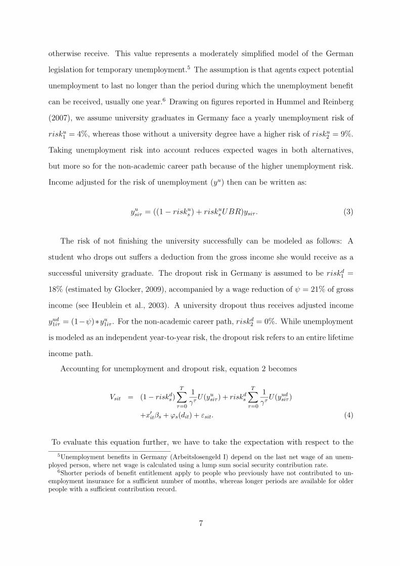
Income adjusted for the risk of unemployment (yu) then can be written as:

yusiτ = ((1 − risku

s ) + riskusUBR)ysiτ . (3)

The risk of not finishing the university successfully can be modeled as follows: A

student who drops out suffers a deduction from the gross income she would receive as a

successful university graduate. The dropout risk in Germany is assumed to be riskd1 =

18% (estimated by Glocker, 2009), accompanied by a wage reduction of ψ = 21% of gross

income (see Heublein et al., 2003). A university dropout thus receives adjusted income

yud1iτ = (1−ψ)∗yu

1iτ . For the non-academic career path, riskd2 = 0%. While unemployment

is modeled as an independent year-to-year risk, the dropout risk refers to an entire lifetime

income path.

Accounting for unemployment and dropout risk, equation 2 becomes

Vsit = (1 − riskds )

T∑

τ=0

1

γτU(yu

siτ ) + riskds

T∑

τ=0

1

γτU(yud

siτ )

+x′itβs + ϕs(dit) + εsit. (4)

To evaluate this equation further, we have to take the expectation with respect to the

5Unemployment benefits in Germany (Arbeitslosengeld I) depend on the last net wage of an unem-ployed person, where net wage is calculated using a lump sum social security contribution rate.

6Shorter periods of benefit entitlement apply to people who previously have not contributed to un-employment insurance for a sufficient number of months, whereas longer periods are available for olderpeople with a sufficient contribution record.

7

random variables ysiτ :

E(Vsit) = (1 − riskds )

T∑

τ=0

1

γτEτ [U(yu

siτ )] + riskds

T∑

τ=0

1

γτEτ

[

U(yudsiτ )]

+x′itβs + ϕs(dit) + εsit. (5)

The expectation of U(ysiτ ) can be approximated by a second-order Taylor series expansion

around µsiτ = E(ysiτ ):

E(U(ysiτ )) ≈ U(µsiτ ) + U ′(µsiτ )E(ysiτ − µsiτ ) +1

2U ′′(µsiτ )E((ysiτ − µsiτ )

2)

= U(µsiτ ) +1

2U ′′(µsiτ )σ

2siτ , (6)

where σ2siτ = V ar(ysiτ ). We must specify a functional form for U(.). In the following,

we assume a constant relative risk aversion (CRRA), as in Hartog and Vijverberg (2007),

which implies that the utility function must satisfy

−yU′′(y)

U ′(y)= ρ, (7)

where the parameter ρ is the coefficient of CRRA (Pratt, 1964).7 The utility function we

choose satisfies the CRRA condition and is increasing in the money (U ′(ysiτ ) > 0):

U(ysiτ ) =

αy1−ρsiτ

1−ρ, if ρ 6= 1.

α ln ysiτ , if ρ = 1.

(8)

This specification therefore implies a risk preference for ρ < 0, risk neutrality for ρ = 0,

and risk aversion for ρ > 0. The structural risk preference parameter ρ will be estimated

econometrically, along with the coefficients of risk-adjusted income α and the control

variables using the maximum likelihood method.

7Alternatively we could assume constant absolute risk aversion (CARA). The advantage of the CARAutility is that a closed-form representation of expected utility exists if y is normally distributed, and noTaylor approximation is needed. Prior literature prefers CRRA though as the more realistic specification,as exemplified by Keane and Wolpin (2001), Sauer (2004), Belzil and Hansen (2004), and Brodaty et al.(2006).

8

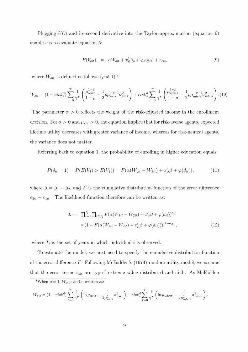
Plugging U(.) and its second derivative into the Taylor approximation (equation 6)

enables us to evaluate equation 5:

E(Vsit) = αWsit + x′itβs + ϕs(dit) + εsit, (9)

where Wsit is defined as follows (ρ 6= 1):8

Wsit = (1 − riskds )

T∑

τ=0

1

γτ

(

µ1−ρusiτ

1 − ρ− 1

2ρµ

−ρ−1usiτ σ2

usiτ

)

+ riskds

T∑

τ=0

1

γτ

(

µ1−ρudsiτ

1 − ρ− 1

2ρµ

−ρ−1udsiτ σ2

udsiτ

)

.(10)

The parameter α > 0 reflects the weight of the risk-adjusted income in the enrollment

decision. For α > 0 and µsiτ > 0, the equation implies that for risk-averse agents, expected

lifetime utility decreases with greater variance of income, whereas for risk-neutral agents,

the variance does not matter.

Referring back to equation 1, the probability of enrolling in higher education equals:

P (δit = 1) = P (E(V1) > E(V2)) = F (α(W1it −W2it) + x′itβ + ϕ(dit)), (11)

where β = β1 − β2, and F is the cumulative distribution function of the error difference

ε2it − ε1it . The likelihood function therefore can be written as:

L =∏N

i=1

∏

t∈TiF (α(W1it − W2it) + x′

itβ + ϕ(dit))δit

× (1 − F (α(W1it − W2it) + x′itβ + ϕ(dit)))

(1−δit) , (12)

where Ti is the set of years in which individual i is observed.

To estimate the model, we next need to specify the cumulative distribution function

of the error difference F . Following McFadden’s (1974) random utility model, we assume

that the error terms εsit are type-I extreme value distributed and i.i.d.. As McFadden

8When ρ = 1, Wsit can be written as:

Wsit = (1 − riskd

s)

T∑

τ=0

1

γτ

(

lnµusiτ − 1

2µ2

usiτ

σ2

usiτ

)

+ riskd

s

T∑

τ=0

1

γτ

(

lnµudsiτ − 1

2µ2

udsiτ

σ2

udsiτ

)

.

9

shows, F is therefore the cumulative logistic probability distribution function.

To predict the future wages, we make several additional assumptions about the two

different career paths. The first assumption relates to income while studying at a uni-

versity. We assume that it takes five years to graduate, which is the approximate mean

in Germany. Because students generally receive monetary transfers, whether from their

parents or as student aid from the government, assuming no income during university at-

tendance would be unrealistic. Instead, we assume that these transfers equal the officially

announced minimum cost of living, which each student is entitled to receive according

to German legislation. During the observation period, these costs were 565 EUR per

month (e.g., Deutscher Bundestag, 2007). We distinguish between students who receive

this income from their own or their parents’ wealth and students who rely on student aid.

Although the amount of income remains the same, transfers from parents versus student

aid are subject to different repayment rules. We therefore assume no repayments if the

income is drawn from the students’ own or their parents’ wealth, whereas students who

draw money from student aid must consider repayment obligations when calculating their

expected lifetime utility. The German Federal Training Assistance Scheme states that

half of the amount of student aid received must be repaid (interest free) as soon as the

borrower’s monthly net income exceeds 1040 EUR. The other half is a subsidy. We model

the eligibility and repayment rules for student aid accordingly. Furthermore, we realize

that many university students work in some kind of part-time job. As university students

already “work” full-time on their education and additional moonlighting further reduces

leasure time, we assume the additional utility from this moonlighting is small and can be

neglected when comparing lifetime utility between the academic and non-academic career

paths.

3 Data

This analysis is based on the German Socio-Economic Panel (SOEP) which is provided by

the German Institute for Economic Research (DIW Berlin). The SOEP is a representative

10

yearly panel survey that gathers detailed information about the socio-economic situation

of (currently) more than 21,000 persons living in approximately 12,000 households in

Germany. Wagner et al. (2007) provide a detailed description of the SOEP. This analysis

draws on the most recent waves (2002 to 20079). One of the advantages of the SOEP is that

in addition to the information collected in the annual interviews, it provides retrospective

information about the respondents’ youth and socialization period, such as school grades,

which are important control variables in the university enrollment model.

We estimate the university enrollment model for the subsample of secondary school

graduates who have obtained a university admission qualification (Abitur/Fachabitur)

and are between 18 and 25 years of age (1,144 observations). Table B1 in the Appendix

lists the descriptive statistics about these potential university entrants, and Table B2

shows descriptive statistics for the full sample used to estimate earnings. We estimate

level and variance of wages separately for men and women because of the well-documented

differences in male and female wage equations. All monetary variables, and therefore all

monetary results, are deflated by the Consumer Price Index (2000 = 100).

4 Estimation of Expectation and Variance of

Earnings

The first step in our analysis of the enrollment decision is to predict individual wage

profiles and the variance of wages over lifetime in the alternative states, with and without

university degrees. In this section, we present the wage and variance estimations, which

are based on the full sample of working-age people.

4.1 Selection

To control for selection effects in the earnings regressions, we apply the Heckman-Lee

method of estimating simultaneous equations with multiple sample selection. The first

9The 2007 wave is used to obtain retrospective income information for 2006 only.

11

selection equation is based on each person’s educational attainment, since we want to

estimate wages separately for academic and non-academic careers. The second selection

occurs because we only observe wages for people who are working. Ignoring these two

selection processes would lead to a selectivity bias in the wage equation (e.g. Fishe

et al., 1981). The first selection equation captures the individual choice to be a university

graduate:

I∗1it = z1itη1 + v1it, (13)

with

I1it =

1, if I∗1it > 0.

0, else.

(14)

The second selection equation models the person’s decision to work:

I∗2it = z2itη2 + I1itι+ v2it, (15)

with

I2it =

1, if I∗2it > 0,

0, else.

(16)

The vector z1it includes only information that is available to the person at the time

of the enrollment decision, such as most recent high-school grades in German and math,

the degree to which parents showed interest in the graduate’s school performance, size of

the city in which the person grew up, parents’ high-school degree and employment status,

and whether the parents were born in Germany. The vector z2it in the work participa-

tion equations features relevant contemporaneous information: age and unemployment

experience (level and square terms), region, education, unemployment rate in the region,

year fixed effects, and whether the individual is married, has young children, was born in

Germany, or is physically handicapped.

We allow the two selection processes to correlate, as is reflected in the error terms

12

(cov(v1it, v2it) = ρv1itv2it6= 0).

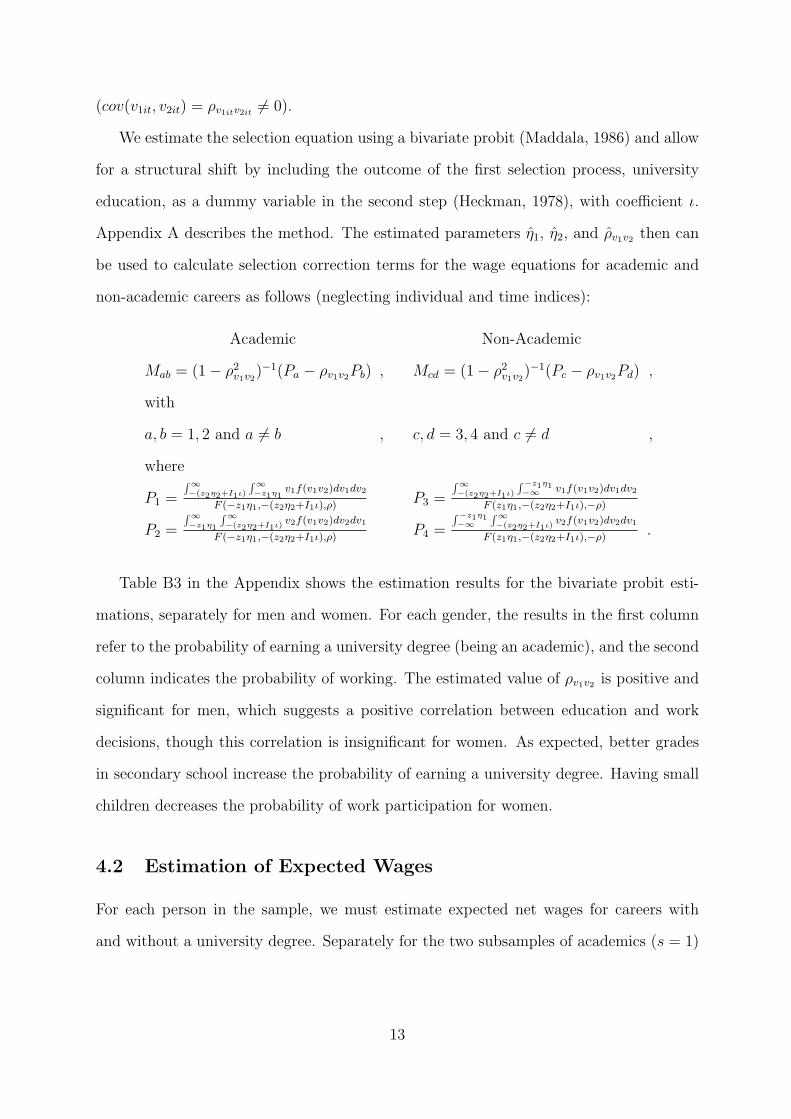
We estimate the selection equation using a bivariate probit (Maddala, 1986) and allow

for a structural shift by including the outcome of the first selection process, university

education, as a dummy variable in the second step (Heckman, 1978), with coefficient ι.

Appendix A describes the method. The estimated parameters η1, η2, and ρv1v2 then can

be used to calculate selection correction terms for the wage equations for academic and

non-academic careers as follows (neglecting individual and time indices):

Academic Non-Academic

Mab = (1 − ρ2v1v2

)−1(Pa − ρv1v2Pb) , Mcd = (1 − ρ2v1v2

)−1(Pc − ρv1v2Pd) ,

with

a, b = 1, 2 and a 6= b , c, d = 3, 4 and c 6= d ,

where

P1 =∫∞

−(z2η2+I1ι)

∫∞

−z1η1v1f(v1v2)dv1dv2

F (−z1η1,−(z2η2+I1ι),ρ)P3 =

∫∞

−(z2η2+I1ι)

∫ −z1η1−∞ v1f(v1v2)dv1dv2

F (z1η1,−(z2η2+I1ι),−ρ)

P2 =∫∞

−z1η1

∫∞

−(z2η2+I1ι) v2f(v1v2)dv2dv1

F (−z1η1,−(z2η2+I1ι),ρ)P4 =

∫ −z1η1−∞

∫∞

−(z2η2+I1ι) v2f(v1v2)dv2dv1

F (z1η1,−(z2η2+I1ι),−ρ).

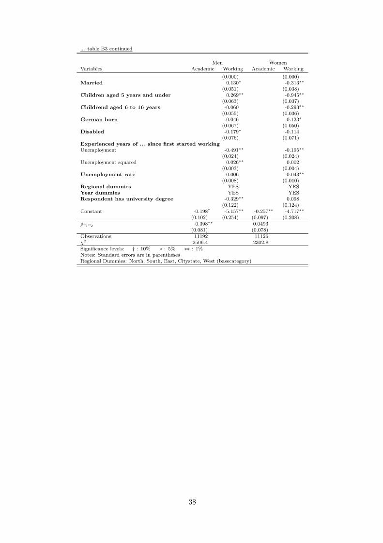
Table B3 in the Appendix shows the estimation results for the bivariate probit esti-

mations, separately for men and women. For each gender, the results in the first column

refer to the probability of earning a university degree (being an academic), and the second

column indicates the probability of working. The estimated value of ρv1v2 is positive and

significant for men, which suggests a positive correlation between education and work

decisions, though this correlation is insignificant for women. As expected, better grades

in secondary school increase the probability of earning a university degree. Having small

children decreases the probability of work participation for women.

4.2 Estimation of Expected Wages

For each person in the sample, we must estimate expected net wages for careers with

and without a university degree. Separately for the two subsamples of academics (s = 1)

13

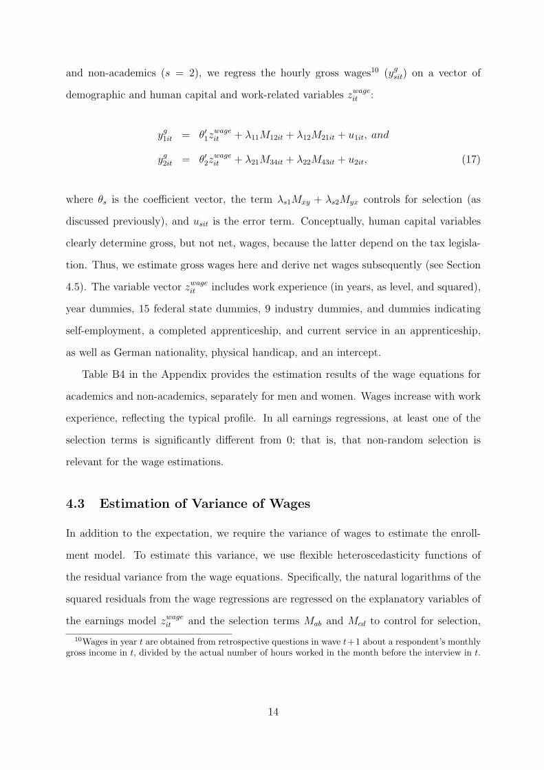
and non-academics (s = 2), we regress the hourly gross wages10 (ygsit) on a vector of

demographic and human capital and work-related variables zwageit :

yg1it = θ′1z

wageit + λ11M12it + λ12M21it + u1it, and

yg2it = θ′2z

wageit + λ21M34it + λ22M43it + u2it, (17)

where θs is the coefficient vector, the term λs1Mxy + λs2Myx controls for selection (as

discussed previously), and usit is the error term. Conceptually, human capital variables

clearly determine gross, but not net, wages, because the latter depend on the tax legisla-

tion. Thus, we estimate gross wages here and derive net wages subsequently (see Section

4.5). The variable vector zwageit includes work experience (in years, as level, and squared),

year dummies, 15 federal state dummies, 9 industry dummies, and dummies indicating

self-employment, a completed apprenticeship, and current service in an apprenticeship,

as well as German nationality, physical handicap, and an intercept.

Table B4 in the Appendix provides the estimation results of the wage equations for

academics and non-academics, separately for men and women. Wages increase with work

experience, reflecting the typical profile. In all earnings regressions, at least one of the

selection terms is significantly different from 0; that is, that non-random selection is

relevant for the wage estimations.

4.3 Estimation of Variance of Wages

In addition to the expectation, we require the variance of wages to estimate the enroll-

ment model. To estimate this variance, we use flexible heteroscedasticity functions of

the residual variance from the wage equations. Specifically, the natural logarithms of the

squared residuals from the wage regressions are regressed on the explanatory variables of

the earnings model zwageit and the selection terms Mab and Mcd to control for selection,

10Wages in year t are obtained from retrospective questions in wave t+1 about a respondent’s monthlygross income in t, divided by the actual number of hours worked in the month before the interview in t.

14

separately for academics and non-academics:

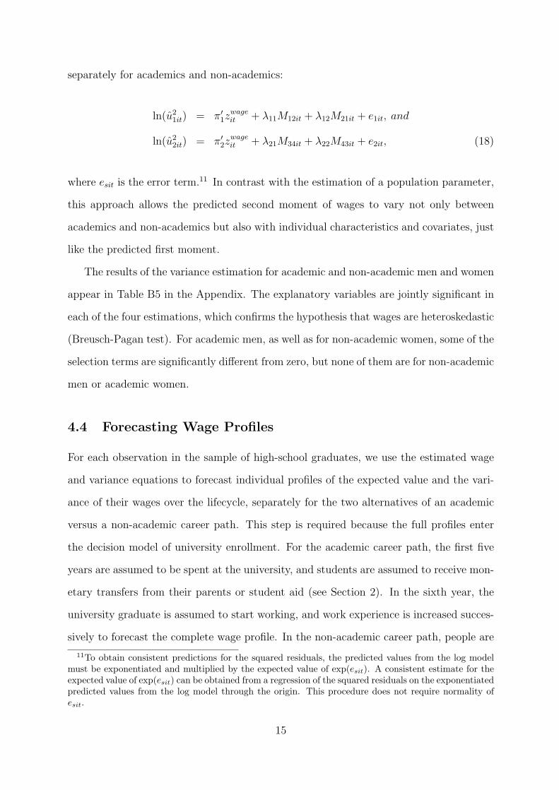
ln(u21it) = π′

1zwageit + λ11M12it + λ12M21it + e1it, and

ln(u22it) = π′

2zwageit + λ21M34it + λ22M43it + e2it, (18)

where esit is the error term.11 In contrast with the estimation of a population parameter,

this approach allows the predicted second moment of wages to vary not only between

academics and non-academics but also with individual characteristics and covariates, just

like the predicted first moment.

The results of the variance estimation for academic and non-academic men and women

appear in Table B5 in the Appendix. The explanatory variables are jointly significant in

each of the four estimations, which confirms the hypothesis that wages are heteroskedastic

(Breusch-Pagan test). For academic men, as well as for non-academic women, some of the

selection terms are significantly different from zero, but none of them are for non-academic

men or academic women.

4.4 Forecasting Wage Profiles

For each observation in the sample of high-school graduates, we use the estimated wage

and variance equations to forecast individual profiles of the expected value and the vari-

ance of their wages over the lifecycle, separately for the two alternatives of an academic

versus a non-academic career path. This step is required because the full profiles enter

the decision model of university enrollment. For the academic career path, the first five

years are assumed to be spent at the university, and students are assumed to receive mon-

etary transfers from their parents or student aid (see Section 2). In the sixth year, the

university graduate is assumed to start working, and work experience is increased succes-

sively to forecast the complete wage profile. In the non-academic career path, people are

11To obtain consistent predictions for the squared residuals, the predicted values from the log modelmust be exponentiated and multiplied by the expected value of exp(esit). A consistent estimate for theexpected value of exp(esit) can be obtained from a regression of the squared residuals on the exponentiatedpredicted values from the log model through the origin. This procedure does not require normality ofesit.

15

assumed to start working right away, and work experience is increased from the first year

on. We assume that those who have not yet finished an apprenticeship plan to pursue an

apprenticeship during the first two years of their non-academic career path. In the wage

and variance equations, we capture lower wages during the apprenticeship with a dummy

variable indicating that someone is currently an apprentice (This variable is negative and

significant in the wage equation; see Table B4). After two years, we assume the appren-

ticeship is finished. When forecasting the wage profiles, in addition to increasing each

person’s work experience and adjusting the information about apprenticeships, we assign

the marital status and number of children information, as well as industry sectors and

self-employment, according to the aggregate distributions, conditional on age and gender.

The end of the individual time horizon occurs at the age of 65 years, the legal retirement

age in Germany during the observation period.

4.5 Microsimulation Model of Income Taxation

Because individual utility depends on net (after-tax) income, the relevant variables in the

enrollment model refer to the expected value and the variance of net wages. To derive

the net from the gross wages, we use a microsimulation model of the German income tax

and social security system. Based on a taxpayer’s gross income, age, region of residence

(there are some regional specifics in the relevant laws), and the legislation in the year of

observation, the tax model calculates the income tax according to the progressive German

income tax schedule, the solidarity surcharge, the social security contributions (i.e., con-

tributions to statutory pension, health, long-term care, and unemployment insurance),

and finally net income.12 The flat tax reform scenarios can be simulated by changing the

parameters of the income tax schedule.

Because we predict gross incomes for the future of current high-school graduates, the

household context (marital status, spouse’s income, number of children) and other relevant

12We convert estimated real hourly gross wages into nominal yearly gross earnings for these calculations,and the resulting nominal yearly net earnings are converted back to real hourly net wages, using theaverage number of hours worked in the sample and the Consumer Price Index.

16

information, such as extraordinary future expenses at the time when gross incomes will be

earned and taxed, are unknown. In this respect, this application of microsimulation differs

from others where the full information available in a dataset about the actual current

household context, incomes, and expenses, can be used for a full household-specific tax-

benefit simulation, as in the tax-benefit model STSM (Steiner et al., 2008). Here, instead,

for simplicity, we assume that the net incomes are calculated for an unmarried person

without children, who does not receive one-off payments and does not pay church tax.

The assumption of being unmarried has the same tax implications as the assumption of

being married to a spouse at the same income level. Net income is then derived exactly

equal to the net income paid to an employee after the deduction of the wage withholding

tax, which is equivalent to assuming that someone does not file an income tax report. This

procedure takes into account the provisional allowance and the allowance for professional

expenses, assuming that actual expenses do not exceed these lump sum allowances. It

seems plausible that high-school graduates, who are usually unmarried and in most cases

do not yet have children, make similar simplifying assumptions when they calculate their

future taxes and social security contributions.

5 Estimation Results of the Enrollment Decision

Model

Table 1 provides the estimation results of the structural enrollment decision model. The

four columns provide the results from different specifications of the discount parameter

γ, which is set at 1.02, 1.05, 1.08, and 1.1, respectively. In general, the results are not

sensitive to the choice of γ.

The point estimate for the structural parameter of constant relative risk aversion ρ is

approximately 0.1 for all γ. It is significant at the 10% level except for γ = 1.02. The

positive ρ indicates risk-averse agents, though the degree of risk aversion is low. Holt

and Laury (2002) estimate a higher degree of risk aversion, that is, around 0.3-0.5. The

17

agents in our sample may be less risk averse than the population at large because of their

particularly young age at the time of their decision about university enrollment; Dohmen

et al. (forthcoming) provide some evidence that risk aversion increases with age.

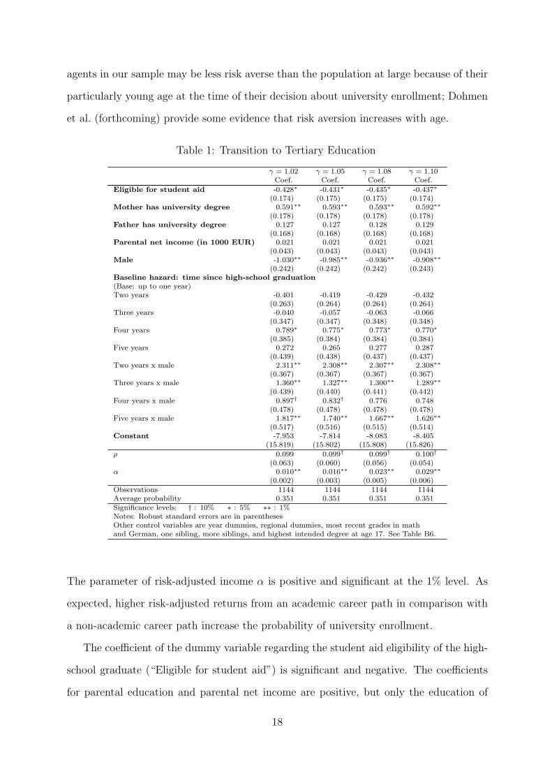
Table 1: Transition to Tertiary Education

γ = 1.02 γ = 1.05 γ = 1.08 γ = 1.10Coef. Coef. Coef. Coef.

Eligible for student aid -0.428∗ -0.431∗ -0.435∗ -0.437∗

(0.174) (0.175) (0.175) (0.174)Mother has university degree 0.591∗∗ 0.593∗∗ 0.593∗∗ 0.592∗∗

(0.178) (0.178) (0.178) (0.178)Father has university degree 0.127 0.127 0.128 0.129

(0.168) (0.168) (0.168) (0.168)Parental net income (in 1000 EUR) 0.021 0.021 0.021 0.021

(0.043) (0.043) (0.043) (0.043)Male -1.030∗∗ -0.985∗∗ -0.936∗∗ -0.908∗∗

(0.242) (0.242) (0.242) (0.243)Baseline hazard: time since high-school graduation(Base: up to one year)Two years -0.401 -0.419 -0.429 -0.432

(0.263) (0.264) (0.264) (0.264)Three years -0.040 -0.057 -0.063 -0.066

(0.347) (0.347) (0.348) (0.348)Four years 0.789∗ 0.775∗ 0.773∗ 0.770∗

(0.385) (0.384) (0.384) (0.384)Five years 0.272 0.265 0.277 0.287

(0.439) (0.438) (0.437) (0.437)Two years x male 2.311∗∗ 2.308∗∗ 2.307∗∗ 2.308∗∗

(0.367) (0.367) (0.367) (0.367)Three years x male 1.360∗∗ 1.327∗∗ 1.300∗∗ 1.289∗∗

(0.439) (0.440) (0.441) (0.442)Four years x male 0.897† 0.832† 0.776 0.748

(0.478) (0.478) (0.478) (0.478)Five years x male 1.817∗∗ 1.740∗∗ 1.667∗∗ 1.626∗∗

(0.517) (0.516) (0.515) (0.514)Constant -7.953 -7.814 -8.083 -8.405

(15.819) (15.802) (15.808) (15.826)

ρ 0.099 0.099† 0.099† 0.100†

(0.063) (0.060) (0.056) (0.054)α 0.010∗∗ 0.016∗∗ 0.023∗∗ 0.029∗∗

(0.002) (0.003) (0.005) (0.006)Observations 1144 1144 1144 1144Average probability 0.351 0.351 0.351 0.351Significance levels: † : 10% ∗ : 5% ∗∗ : 1%Notes: Robust standard errors are in parenthesesOther control variables are year dummies, regional dummies, most recent grades in mathand German, one sibling, more siblings, and highest intended degree at age 17. See Table B6.

The parameter of risk-adjusted income α is positive and significant at the 1% level. As

expected, higher risk-adjusted returns from an academic career path in comparison with

a non-academic career path increase the probability of university enrollment.

The coefficient of the dummy variable regarding the student aid eligibility of the high-

school graduate (“Eligible for student aid”) is significant and negative. The coefficients

for parental education and parental net income are positive, but only the education of

18

the mother is significantly different from zero. All these variables capture the social back-

ground of a person and are hard to interpret separately. Student aid eligibility depends

mostly on parental income and wealth, which in turn is highly correlated with education.

Together, the results indicate that children from a socially disadvantaged background

(i.e., eligible for student aid, low parental income and education) are less likely to enroll

at a university. This assertion is consistent with the existence of credit constraints, but

it could also indicate that better educated and richer parents are able to provide more

immaterial support, encouragement, and insurance to their children.

Gender differences are captured by the “male” dummy, as well as its interaction with

the dummy variables indicating the time elapsed since high-school graduation. The results

show that men exhibit a lower enrollment probability in the first year after high-school

graduation but a higher one in the following years, which reflects that German young men

often serve a mandatory military or alternative civil service term immediately after their

high-school graduation.

The estimated coefficients of the additional control variables, in Table B6, indicate that

good grades at the age of 17 years have a positive effect on the probability of university

enrollment. The same holds for the variable indicatig if a future high-school graduate

had the intention at the age of 17 years to obtain a university degree in the future. This

variable might capture preferences for certain career choices that form at an earlier age.

Because our estimates are not sensitive to the choice of γ, in the following we focus

on the estimates derived using the specification for which γ is 1.05. We conducted all the

calculations and simulations for the other choices of γ as well and consistently find very

similar results, which are available from the authors upon request.

At the mean values of the explanatory variables, the estimated hazard of university

enrollment for a high-school graduate in the sample in a given year is 35.1%. The cumu-

lative probability of enrollment after five years is estimated to be 70%. These numbers

do not significantly differ from official statistics, which report an average yearly univer-

sity enrollment rate of 37% of a German high-school graduate and reveal that 75% of

19

the graduates enroll within five years of leaving high-school (Statistisches Bundesamt,

2007). Steiner and Wrohlich (2008) estimate very similar probabilities on the basis of a

non-structural model of university enrollment, also using SOEP data.

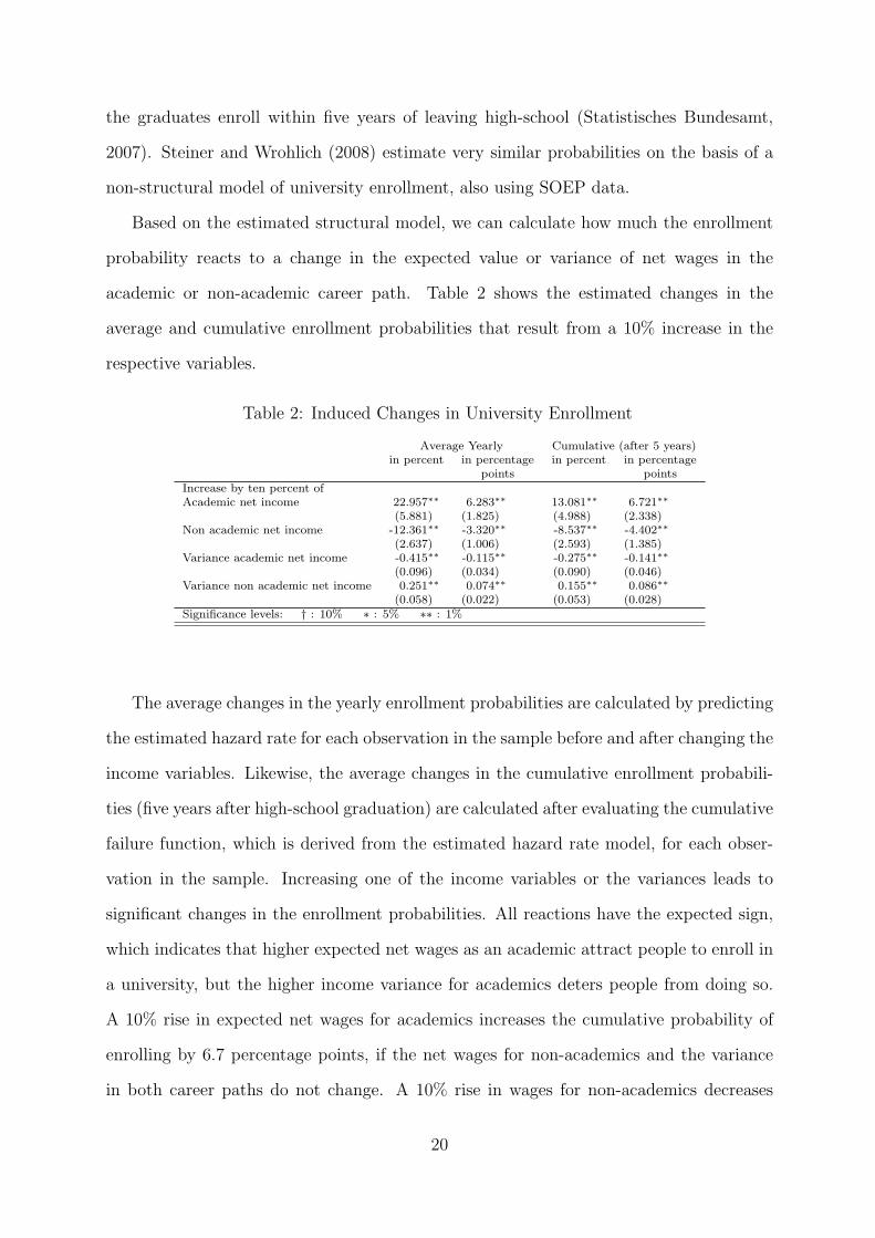
Based on the estimated structural model, we can calculate how much the enrollment

probability reacts to a change in the expected value or variance of net wages in the

academic or non-academic career path. Table 2 shows the estimated changes in the

average and cumulative enrollment probabilities that result from a 10% increase in the

respective variables.

Table 2: Induced Changes in University Enrollment

Average Yearly Cumulative (after 5 years)in percent in percentage in percent in percentage

points pointsIncrease by ten percent ofAcademic net income 22.957∗∗ 6.283∗∗ 13.081∗∗ 6.721∗∗

(5.881) (1.825) (4.988) (2.338)Non academic net income -12.361∗∗ -3.320∗∗ -8.537∗∗ -4.402∗∗

(2.637) (1.006) (2.593) (1.385)Variance academic net income -0.415∗∗ -0.115∗∗ -0.275∗∗ -0.141∗∗

(0.096) (0.034) (0.090) (0.046)Variance non academic net income 0.251∗∗ 0.074∗∗ 0.155∗∗ 0.086∗∗

(0.058) (0.022) (0.053) (0.028)Significance levels: † : 10% ∗ : 5% ∗∗ : 1%

The average changes in the yearly enrollment probabilities are calculated by predicting

the estimated hazard rate for each observation in the sample before and after changing the

income variables. Likewise, the average changes in the cumulative enrollment probabili-

ties (five years after high-school graduation) are calculated after evaluating the cumulative

failure function, which is derived from the estimated hazard rate model, for each obser-

vation in the sample. Increasing one of the income variables or the variances leads to

significant changes in the enrollment probabilities. All reactions have the expected sign,

which indicates that higher expected net wages as an academic attract people to enroll in

a university, but the higher income variance for academics deters people from doing so.

A 10% rise in expected net wages for academics increases the cumulative probability of

enrolling by 6.7 percentage points, if the net wages for non-academics and the variance

in both career paths do not change. A 10% rise in wages for non-academics decreases

20

the probability by 4.4 percentage points, ceteris paribus. The elasticities are not equal

in absolute terms because of the different mean variances in the two career paths. If

the wage variance in the academic path increases by 10%, the enrollment probability de-

creases by 0.14 percentage points, everything else being equal. An increase in the wage

variance in the non-academic path leads to an increase in the enrollment probability by

0.09 percentage points.

6 Simulation of Flat-Rate Tax Reform

As shown in the previous section, expectations about future net income influence the

university enrollment decision. Therefore the estimated structural model can be applied

to simulate the effects of tax policy scenarios on university enrollment. As an illustrative

example, we analyze the effects of two revenue-neutral flat-rate tax scenarios. Flat-rate

taxes have been widely discussed in Germany; Kirchhoff (2003), Mitschke (2004), and

the Council of Economic Advisors to the Ministry of Finance (2004) all have presented

proposals for tax policy reforms with (almost) flat-rate schedules.

In the strictest sense, a flat tax is a uniform tax rate on the total tax base. In practice,

a flat income tax rate is usually combined with a basic tax allowance, which leads to an

implicitly progressive tax schedule. Thus, if the tax base is left unchanged, a flat-rate tax

policy can be defined by two parameters, the uniform tax rate and the basic allowance.

Fuest et al. (2008) analyze the distributional and labor supply effects of two flat tax

scenarios for Germany using a microsimulation model. The first policy is defined by a low

tax rate and a low basic allowance (scenario “Low-Low”), whereas the second features

higher values for the two parameters (scenario “High-High”). These authors balance the

parameters of each scenario to establish revenue neutrality in their simulation for 2007,

assuming that there are no behavioral responses such as labor supply reactions. In the

scenario “Low-Low” (LL), the basic allowance remains unchanged at 7,664 EUR, and the

tax rate that establishes revenue neutrality is 26.9%. In the scenario “High-High” (HH),

a higher basic allowance of 10,700 EUR and a higher revenue neutral flat tax rate of

21

31.9% are chosen.13 Scenario HH is implicitly more progressive than scenario LL because

of its high basic allowance. Thus, it is more similar to Germany’s current progressive tax

schedule, whereas in scenario LL effective tax rates are significantly flatter.

The aim of this section is to estimate the effects of the two flat tax policies defined by

Fuest et al. (2008) on university enrollment. The baseline scenario is the actual German

tax legislation of 2005 and 2006.14 Correspondingly, we use the high-school graduates

observed in 2005 or 2006 to simulate the effects of the reforms. Using our microsimulation

model, we calculate the first and second moment of net (after-tax) income in the baseline

and the two alternative policy scenarios, based on our estimates of gross income, and then

apply the estimated structural model of university enrollment to simulate the effects of

the changes in the expectation and variance of net income.

The results are presented in Table 3 along with the tax parameters that define the

scenarios. In the baseline scenario (first row), the average yearly probability of university

enrollment is estimated to be 32.0% for female and 31.6% for male high-school graduates.15

The model accounts for gender differences by employing gender-specific baseline hazards,

and the other explanatory variables control for different endowments.

We focus on the simulation results for the flat tax scenario LL first, which leaves the

basic tax allowance unchanged. The results indicate that scenario LL makes university

education more attractive for male high-school graduates. The average yearly probability

of enrollment for young men significantly increases from 31.6% to 33.1% (+1.4 percentage

points). The cumulative probability of enrollment five years after high-school graduation

also increases significantly by 1.8 percentage points, which corresponds to a relative in-

13The distinctive feature of scenario HH is that it does not change the Gini index of inequality comparedwith a situation without the reform, according to the simulations of Fuest et al. (2008), again withoutbehavioral responses. This is explained by the high basic allowance, which reduces taxes for low incomepeople. The Council of Economic Advisors to the Ministry of Finance (2004) suggested a similar (butnot revenue-neutral) flat tax with a basic allowance of 10,000 EUR and a tax rate of 30%.

14This is after the full implementation of the Tax Reform 2000, which reduced the general statutoryincome tax rates and simultaneously increased the basic tax allowance in three steps between 1 January2001 and 1 January 2005. The top marginal income tax rate dropped from 51% in 2000 to 42% in 2005,the lowest marginal tax rate from 22.9% to 15%, and the basic allowance increased from 6,902 EUR to7,664 EUR (for an unmarried individual); see also Fossen (2009).

15This estimate, which is based on the pooled sample of 2005 and 2006, is somewhat lower than theestimate based on 2002-2006, which was reported in section 5.

22

crease in the cumulative enrollment probability by 3.1%. The change in the cumulative

probability is directly relevant to policy, because it indicates how much the share of men

who decide to study at all would increase (very few people enter university later than

after five years after their high-school graduation).

Table 3: Simulated Changes in the Probability of University Enrollment

Male High-School Graduates Female High-School Graduates Tax ParametersAverage Cumulative Average Cumulative Basic Marginal

Probability Probability Probability Probability Allowance Tax Rate1

(yearly) (after 5 years) (yearly) (after 5 years) (EUR) (percent)

Baseline ScenarioEnrollment Probability 31.635∗∗ 58.880∗∗ 31.952∗∗ 75.092∗∗ 7,664 15-42

(8.788) (12.020) (9.072) (9.585)

Low-LowEnrollment Probability 33.078∗∗ 60.728∗∗ 31.118∗∗ 74.543∗∗ 7,664 26.9

(9.010) (11.889) (8.964) (9.800)Difference in percentage 1.443∗ 1.848∗ -0.835∗∗ -0.549points (effect of reform) (0.612) (0.875) (0.323) (0.401)

High-HighEnrollment Probability 31.281∗∗ 58.400∗∗ 31.523∗∗ 74.548∗∗ 10,700 31.9

(8.734) (12.047) (8.978) (9.662)Difference in percentage -0.354 -0.480 -0.430∗ -0.544∗

points (effect of reform) (0.238) (0.343) (0.199) (0.262)Significance levels: † : 10% ∗ : 5% ∗∗ : 1%Standard errors in parentheses1 plus solidarity surcharge in all scenarios

The simulated effect of scenario LL on young men contrasts with the effect on young

women. The flat tax scenario significantly decreases womens’ average yearly probability

of university enrollment by 0.8 percentage points. There is no significant effect on the

female cumulative enrollment probability, however. Scenario LL may thus induce female

high-school graduates to enter university less quickly, but would not significantly decrease

the number of female university students in the long run.

What explains the different effects of the flat tax scenario on male and female high-

school graduates? The revenue-neutral flat tax reform has two opposing effects. First, the

tax burden decreases for higher and increases for lower incomes (above the allowance), so

an academic career path becomes more attractive (incentive effect of taxation). Second,

the variance of net income increases with a flat tax, which is especially relevant for aca-

demics, who face higher income risk. This effect discourages potential students from an

23

academic career, as it becomes more risky (risk-sharing aspect of progressive taxation).

The simulation results indicate that for men, the positive incentive effect of the flat tax

outweighs the negative risk-sharing effect. For women, it is the other way round. This is

explained by men’s higher wages, especially in the academic career path. The spread be-

tween academic and non-academic average predicted gross wages is 9.11 EUR for men but

only 5.93 EUR for women (see the bottom of Table B4). Because the flat tax reduces the

tax rates for higher incomes, for men, incentives for an academic versus a non-academic

path increase more than for women. In contrast, the spread between the log(variance)

of gross wages in the alternative career paths is 0.89 for women and only 0.76 for men

(Table B5). The flat tax increases the variance of net wages, and this discouraging effect

is stronger for women.

Scenario HH combines a flat tax rate with a basic tax allowance that is almost 40%

higher than in the baseline scenario. It thus not only decreases the tax burden for high

income people, but also for low income people who benefit from the higher allowance. As

the reform scenario is revenue-neutral, people at intermediate income ranges pay more

taxes than in the baseline scenario. The simulation results indicate that scenario HH

has no significant effect on young men’s university enrollment, whereas for young women,

enrollment decreases somewhat, and the decrease is statistically significant. The average

yearly enrollment probability of female high-school graduates decreases by 0.4 percentage

points, and the cumulative enrollment probability after five years by 5.4 percentage points,

which corresponds to a relative decrease by 0.7%. In this scenario, the disadvantage of

the flat tax in terms of higher income risk offsets or even outweighs the incentive effect.

Especially for women, who have lower wages than men, the high basic tax allowance in

this scenario makes the non-academic career path relatively more attractive. The different

results for the two flat tax scenarios highlight the importance of clear definitions when

talking about a flat tax.

To illustrate the simulation results, we use Figure 1 to depict the development of

the cumulative enrollment probabilities in the different tax scenarios during the first five

24

years after high-school graduation, separately for men and women with average observed

characteristics.

7 Conclusion

We estimate a structural microeconometric model of university enrollment, in which high-

school graduates decide to enroll according to their comparison of the present value of the

discounted utility from career paths with and without a university degree. Utility in each

future period depends on not only expected income but also income risk. The expected

value and the variance of wages in the two alternative career paths are estimated individ-

ually, taking into account non-random selection based on multiple correlated criteria.

The estimation results are consistent with expectations. Higher risk-adjusted expected

wages as a university graduate, relative to the alternative, increase the probability of en-

rollment. The Arrow-Pratt coefficient of constant relative risk aversion, which is included

in the structural model as a parameter, is econometrically estimated to be approximately

0.1 and statistically significant. Thus, high-school graduates are risk averse, though to

a low degree, potentially because of their young age. Consequently, a higher variance of

net wages for academics, ceteris paribus, discourages high-school graduates from pursuing

tertiary education.

In contrast to the existing literature considering earnings risk, this analysis acknowl-

edges that after-tax income is relevant for the decision to acquire tertiary education and

takes taxation explicitly into account. Both the incentive effect of taxation – through its

impact on the earnings differential between academic and non-academic career paths –

and the risk-sharing effect – through its impact on earnings risk in the two alternatives –

can be analyzed simultaneously. This method allows us to apply the estimated structural

model to simulate the effect of tax policy reforms on university enrollment.

We apply the estimated model to simulate the effects of two hypothetical revenue-

neutral, flat-rate tax scenarios on university enrollment in Germany. The simulation

results indicate that a revenue-neutral, flat tax scenario with an unchanged basic tax

25

allowance would significantly increase the cumulative probability of university enrollment

for male high-school graduates by 1.8 percentage points (five years after high-school grad-

uation), which corresponds to a relative increase of 3.1%. For men, the positive incentive

effect of the flat tax reform thus outweighs the negative insurance effect. Because of

women’s lower expected wages though, the simulated flat tax scenario with an unchanged

basic allowance would not have a significant effect on the cumulative enrollment proba-

bility of female high-school graduates.

The policy debate about taxation and tertiary education focuses primarily on the

effect of relative levels of net income on incentives for education. However, the findings

from this study suggest that it may be just as important to consider the relative after-tax

income risk associated with academic and non-academic career paths.

26

References

Anderberg, D. (2009): “Optimal policy and the risk properties of human capital recon-

sidered”. Journal of Public Economics, 93:1017–1026.

Anderberg, D. and Andersson, F. (2003): “Investments in human capital, wage uncer-

tainty, and public policy”. Journal of Public Economics, 87:1521–1537.

Belzil, C. and Hansen, J. (2004): “Earnings Dispersion, Risk Aversion and Education”.

Working Papers 0406, Groupe d’Analyse et de Thorie Economique (GATE), Centre na-

tional de la recherche scientifique (CNRS), Universit Lyon 2, Ecole Normale Suprieure.

Brodaty, T., Gary-Bobo, R.J., and Prieto, A. (2006): “Risk Aversion and Human Cap-

ital Investment: A Structural Econometric Model”. CEPR Discussion Papers 5694,

C.E.P.R. Discussion Papers.

Carneiro, P., Hansen, K., and Heckman, J. (2003): “Estimating distributions of treatment

effects with an application to the returns to schooling and measurement of the effects

of uncertainty on college choice”. International Economic Review, 44(2):361–422.

Carneiro, P. and Heckman, J.J. (2002): “The Evidence on Credit Constraints in Post-

Secondary Schooling”. The Economic Journal, 112(482):705–734.

Council of Economic Advisors to the Ministry of Finance (2004): “Flat Tax oder

Duale Einkommensteuer? Zwei Entwurfe zur Reform der deutschen Einkommens-

besteuerung”.

Cunha, F., Heckman, J., and Navarro, S. (2005): “Separating uncertainty from hetero-

geneity in life cycle earnings”. Oxford Economic Papers, 57(2):191–261.

Cunha, F. and Heckman, J.J. (2007): “Identifying and Estimating the Distributions of Ex

Post and Ex Ante Returns to Schooling”. Labour Economics, 14(6):870–893. Education

and Risk - Education and Risk S.I.

27

Deutscher Bundestag (2007): “Siebzehnter Bericht nach 35 des Bundesaus-

bildungsforderungsgesetztes zur Uberprufung der Bedarfssatze, Freibetrage sowie

Vomhundertsatze und Hochstbetrage nach 21 Abs.2.” Deutscher Bundestag, Druck-

sache 16/4123.

Dohmen, T., Falk, A., Huffman, D., Schupp, J., Sunde, U., and Wagner, G.G. (forthcom-

ing): “Individual Risk Attitudes: Measurement, Determinants and Behavioral Conse-

quences”. Forthcoming in: Journal of the European Economic Association.

Eaton, J. and Rosen, H. (1980): “Taxation, human capital and uncertainty”. American

Economic Review, 70(4):705–715.

Fishe, R.P., Trost, R., and Lurie, P.M. (1981): “Labor Force Earnings and College Choice

of Young Women: An Exammination of Selectivity Bias and Comparative Advantage”.

Economics of Education Review, 1(2):169–191.

Fossen, F.M. (2009): “Would a Flat-Rate Tax Stimulate Entrepreneurship in Germany?

A Behavioural Microsimulation Analysis Allowing for Risk”. Fiscal Studies, 30(2):179–

218.

Fuest, C., Peichl, A., and Schaefer, T. (2008): “Is a Flat Tax Reform Feasible in a Grown-

up Democracy of Western Europe? A Simulation Study for Germany”. International

Tax and Public Finance, 15(5):620–636.

Glocker, D. (2009): “The Effect of Student Aid on the Duration of Study”. DIW Discus-

sion Paper 893, German Institute for Economic Research.

Hartog, J. and Serrano, L.D. (2007): “Earnings Risk and Demand for Higher Education:

A Cross-Section Test for Spain”. Journal of Applied Economics, X(1):1–28.

Hartog, J. and Vijverberg, W.P. (2007): “On compensation for risk aversion and skewness

affection in wages”. Labour Economics, 14(6):938–956.

28

Heckman, J.J. (1978): “Dummy Endogenous Variables in a Simultaneous Equation Sys-

tem”. Econometrica, 46(4):931–59.

Heckman, J.J., Lochner, L., and Taber, C. (1998): “Tax Policy and Human-Capital

Formation”. American Economic Review, 88(2):293–97.

Heine, C., Spangenberg, H., and Willich, J. (2008): “Studienberechtigte 2006 ein halbes

Jahr nach Schulabschluss - bergang in Studium, Beruf und Ausbildung”. HIS: Forum

Hochschule.

Heublein, U., Spangenberg, H., and Sommer, D. (2003): “Ursachen des Studienabbruchs-

Analyse 2002”. Technical report, HIS.

Hogan, V. and Walker, I. (2003): “Education Choice under Uncertainty and Public Pol-

icy”. Working Papers 200302, School Of Economics, University College Dublin.

Holt, C.A. and Laury, S.K. (2002): “Risk Aversion and Incentive Effects”. The American

Economic Review, 92(5):1644–1655.

Hummel, M. and Reinberg, A. (2007): “Qualifikationsspezifische Arbeitslosigkeit im Jahr

2005 und die Einfhrung der Hartz-IV-Reform - Empirische Befunde und methodische

Probleme”. IAB Forschungsbericht.

Kane, T.J. (2003): “A Quasi-Experimental Estimate of the Impact of Financial Aid on

College-Going”. Working Paper Series 9703, NBER Working Paper.

Keane, M.P. and Wolpin, K.I. (2001): “The Effect of Parental Transfers and Borrowing

Constraints on Educational Attainment”. International Economic Review, 42(4):1051–

1103.

Kirchhoff, P. (2003): Einkommensteuergesetzbuch Ein Vorschlag zur Reform der

Einkommen− und Korperschaftsteuer. C. F. Muller Verlag, Heidelberg.

Kodde, D. (1986): “Uncertainty and the demand for education”. Review of Economics

and Statistics, 68:460–467.

29

Levhari, D. and Weiss, Y. (1974): “The Effect of Risk on the Investment in Human

Capital”. American Economic Review, 64(6):950–63.

Maddala, G.S. (1986): Limited-dependent and qualitative variables in econometrics.

Number 3 in Econometric Society Monographs. Cambridge University Press.

McFadden, D. (1974): “Conditional Logit Analysis of Qualitative Choice Behavior”. In

P. Zarembka, editor, “Frontiers in Econometrics”, pages 105–142. Academic Press, New

York.

Mitschke, J. (2004): Erneuerung des deutschen Einkommensteuerrechts:

Gesetzestextentwurf und Begrundung. Verlag Otto Schmidt, Cologne.

OECD (2008): Education at a glance 2008. OECD, Paris.

Pratt, J.W. (1964): “Risk Aversion in the Small and in the Large”. Econometrica,

32(1/2):122–136.

Rosenbaum, S. (1961): “Moments of a Truncated Bivariate Normal Distribution”. Journal

of the Royal Statistical Society. Series B (Methodological), 23(2):405–408.

Sauer, R.M. (2004): “Educational Financing and Lifetime Earnings”. Review of Economic

Studies, 71(4):1189–1216.

Shea, J. (2000): “Does parents’ money matter?” Journal of Public Economics, 77(2):155–

184.

Statistisches Bundesamt (2007): Hochschulen auf einen Blick. Wiesbaden.

Steiner, V., Geyer, J., Haan, P., and Wrohlich, K. (2008): “Documentation of the Tax-

Benefit Microsimulation Model STSM: Version 2008”. DIW Data Documentation 31,

German Institute for Economic Research.

Steiner, V. and Wrohlich, K. (2008): “Financial Student Aid and Enrollment into Higher

Education: New Evidence from Germany”. DIW Discussion Paper 805, German Insti-

tute for Economic Research.

30

Wagner, G.G., Frick, J.R., and Schupp, J. (2007): “The German Socio-Economic

Panel Study (SOEP) - Scope, Evolution and Enhancements”. Schmollers Jahrbuch,

127(1):139–169.

Willis, R.J. and Rosen, S. (1979): “Education and Self-Selection”. The Journal of Political

Economy, 87(5):S7–S36.

31

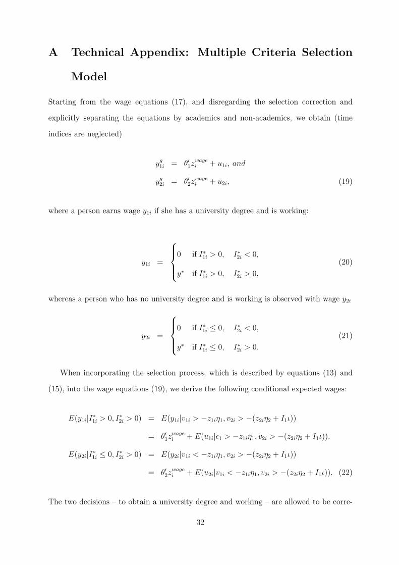
A Technical Appendix: Multiple Criteria Selection

Model

Starting from the wage equations (17), and disregarding the selection correction and

explicitly separating the equations by academics and non-academics, we obtain (time

indices are neglected)

yg1i = θ′1z

wagei + u1i, and

yg2i = θ′2z

wagei + u2i, (19)

where a person earns wage y1i if she has a university degree and is working:

y1i =

0 if I∗1i > 0, I∗2i < 0,

y∗ if I∗1i > 0, I∗2i > 0,

(20)

whereas a person who has no university degree and is working is observed with wage y2i

y2i =

0 if I∗1i ≤ 0, I∗2i < 0,

y∗ if I∗1i ≤ 0, I∗2i > 0.

(21)

When incorporating the selection process, which is described by equations (13) and

(15), into the wage equations (19), we derive the following conditional expected wages:

E(y1i|I∗1i > 0, I∗2i > 0) = E(y1i|v1i > −z1iη1, v2i > −(z2iη2 + I1ι))

= θ′1zwagei + E(u1i|ǫ1 > −z1iη1, v2i > −(z2iη2 + I1ι)).

E(y2i|I∗1i ≤ 0, I∗2i > 0) = E(y2i|v1i < −z1iη1, v2i > −(z2iη2 + I1ι))

= θ′2zwagei + E(u2i|v1i < −z1iη1, v2i > −(z2iη2 + I1ι)). (22)

The two decisions – to obtain a university degree and working – are allowed to be corre-

32

lated. The correlation is reflected in the error terms (cov(v1, v2) = ρv1v2 6= 0). The error

terms are assumed to have a normal distribution with zero mean and var(v1) = var(v2) =

1 (in addition, person indices will be neglected in the following),

u1

u2

v1

v2

∼ N

0,

∑

uu∑

uv

∑

vu∑

vv

Following Maddala (1986), the second term on the right-hand side of equation (22)

can be expressed as:

E(u1|v1 > −z1η1, v2 > −(z2η2 + I1ι)) = λ11M12 + λ12M21

E(u2|v1 < −z1η1, v2 > −(z2η2 + I1ι)) = λ21M34 + λ22M43, (23)

where

λsj = cov(us, vj)

cov(v1, v2) = ρ

Mab = (1 − ρ2)−1(Pa − ρPb)

with a, b = 1, 2 and a 6= b

Mcd = (1 − ρ2)−1(Pc − ρPd)

with c, d = 3, 4 and c 6= d

33

with

P1 =

∫∞

−(z2η2+I1ι)

∫∞

−z1η1v1f(v1v2)dv1dv2

F (−z1η1,−(z2η2 + I1ι), ρ)

P2 =

∫∞

−z1η1

∫∞

−(z2η2+I1ι)v2f(v1v2)dv2dv1

F (−z1η1,−(z2η2 + I1ι), ρ)

P3 =

∫∞

−(z2η2+I1ι)

∫ −z1η1

−∞v1f(v1v2)dv1dv2

F (z1η1,−(z2η2 + I1ι),−ρ)

P4 =

∫ −z1η1

−∞

∫∞

−(z2η2+I1ι)v2f(v1v2)dv2dv1

F (z1η1,−(z2η2 + I1ι),−ρ)

According to Rosenbaum (1961) the truncated bivariate normal distribution can be

solved numerically, which leads to:

M12 =

φ(z1η1)Φ

(

(z2η2+I1ι)−ρ(z1η1)√1−ρ2

)

Φ2(z1η1, z2η2 + I1ι, ρ)

M21 =

φ(z2η2 + I1ι)Φ

(

z1η1−ρ(z2η2+I1ι)√1−ρ2

)

Φ2(z1η1, z2η2 + I1ι, ρ)

M34 =

φ(−z1η1)Φ

(

(z2η2+I1ι)−ρ(−z1η1)√1−ρ2

)

Φ2(−z1η1, z2η2 + I1ι,−ρ)

M43 =

φ(z2η2 + I1ι)Φ

(

−z1η1−ρ(z2η2+I1ι)√1−ρ2

)

Φ2(−z1η1, z2η2 + I1ι,−ρ)

where φ is the standard normal density function, Φ denotes the standard, and Φ2 is the

bivariate normal cumulative distribution. Controlling for the selection terms, the wage

equations can now be expressed in the form of equation (17).

34

B Additional Tables

Table B1: Descriptive Statistics, High-school Graduates

Variable Names Mean Standard Dev.

Eligible for student aid 0.36 0.48Age when finished high school 19.42 1.01Mother holds university degree 0.27 0.44Father holds university degree 0.40 0.49Parental net income (in 1000 EUR) 2.75 1.83Intended a university degree at age 17 0.27 0.44Intended degree at age 17 n.a. 0.59 0.49Respondent has one sibling 0.32 0.47Respondent has more than one sibling 0.09 0.28Finished apprenticeship 0.13 0.33Male 0.49 0.50School grades in German at age 17n.a. 0.36 0.48Very good (1) 0.03 0.17Good (2)) 0.27 0.44Satisfactory (3) 0.26 0.44Poor (4-6) 0.08 0.27School grades in math at age 17n.a. 0.36 0.48Very good (1) 0.06 0.25Good (2) 0.20 0.40Satisfactory (3) 0.22 0.41Poor (4-6) 0.15 0.36Years since high-school graduationOne year 0.42 0.49Two years 0.24 0.43Three years 0.16 0.36Four years 0.11 0.32Five years 0.08 0.27

Observations 1144

35

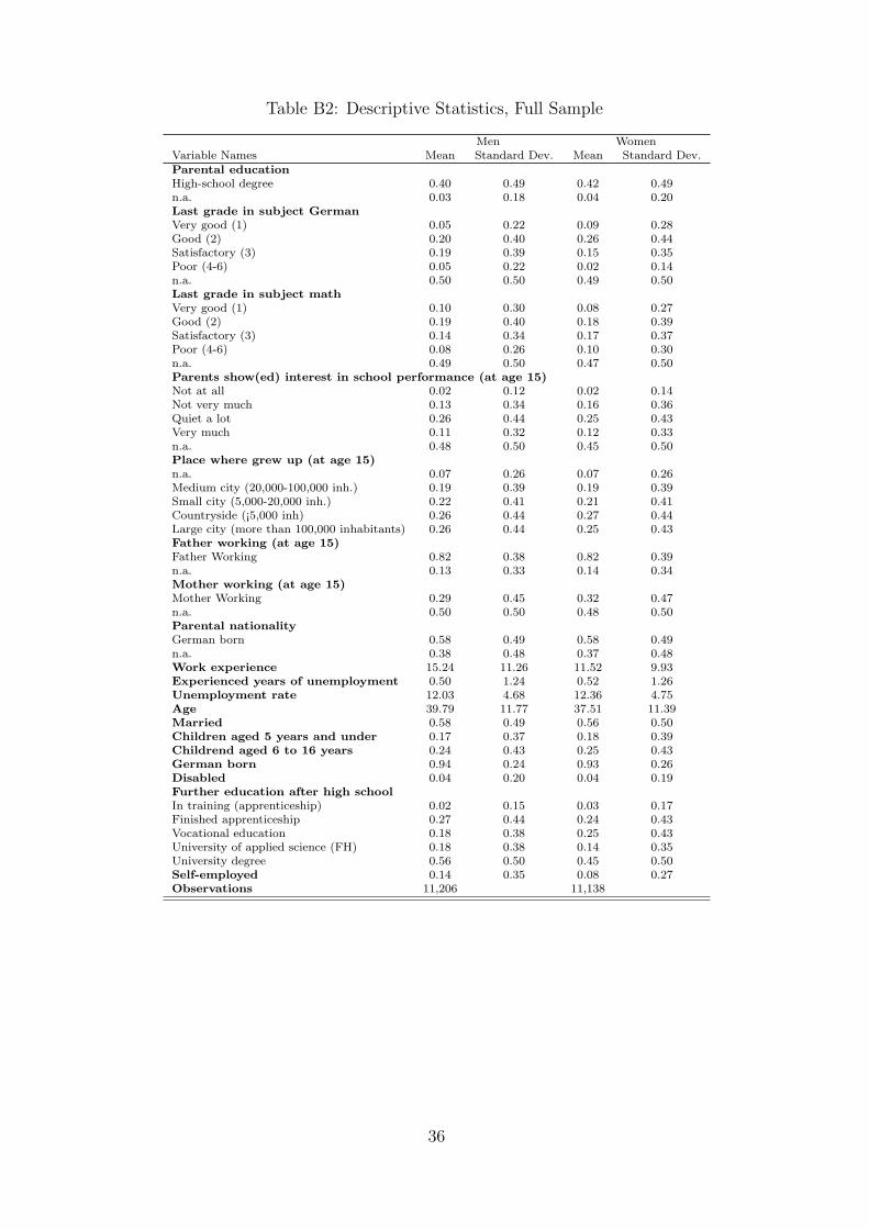
Table B2: Descriptive Statistics, Full Sample

Men WomenVariable Names Mean Standard Dev. Mean Standard Dev.Parental educationHigh-school degree 0.40 0.49 0.42 0.49n.a. 0.03 0.18 0.04 0.20Last grade in subject GermanVery good (1) 0.05 0.22 0.09 0.28Good (2) 0.20 0.40 0.26 0.44Satisfactory (3) 0.19 0.39 0.15 0.35Poor (4-6) 0.05 0.22 0.02 0.14n.a. 0.50 0.50 0.49 0.50Last grade in subject mathVery good (1) 0.10 0.30 0.08 0.27Good (2) 0.19 0.40 0.18 0.39Satisfactory (3) 0.14 0.34 0.17 0.37Poor (4-6) 0.08 0.26 0.10 0.30n.a. 0.49 0.50 0.47 0.50Parents show(ed) interest in school performance (at age 15)Not at all 0.02 0.12 0.02 0.14Not very much 0.13 0.34 0.16 0.36Quiet a lot 0.26 0.44 0.25 0.43Very much 0.11 0.32 0.12 0.33n.a. 0.48 0.50 0.45 0.50Place where grew up (at age 15)n.a. 0.07 0.26 0.07 0.26Medium city (20,000-100,000 inh.) 0.19 0.39 0.19 0.39Small city (5,000-20,000 inh.) 0.22 0.41 0.21 0.41Countryside (¡5,000 inh) 0.26 0.44 0.27 0.44Large city (more than 100,000 inhabitants) 0.26 0.44 0.25 0.43Father working (at age 15)Father Working 0.82 0.38 0.82 0.39n.a. 0.13 0.33 0.14 0.34Mother working (at age 15)Mother Working 0.29 0.45 0.32 0.47n.a. 0.50 0.50 0.48 0.50Parental nationalityGerman born 0.58 0.49 0.58 0.49n.a. 0.38 0.48 0.37 0.48Work experience 15.24 11.26 11.52 9.93Experienced years of unemployment 0.50 1.24 0.52 1.26Unemployment rate 12.03 4.68 12.36 4.75Age 39.79 11.77 37.51 11.39Married 0.58 0.49 0.56 0.50Children aged 5 years and under 0.17 0.37 0.18 0.39Childrend aged 6 to 16 years 0.24 0.43 0.25 0.43German born 0.94 0.24 0.93 0.26Disabled 0.04 0.20 0.04 0.19Further education after high schoolIn training (apprenticeship) 0.02 0.15 0.03 0.17Finished apprenticeship 0.27 0.44 0.24 0.43Vocational education 0.18 0.38 0.25 0.43University of applied science (FH) 0.18 0.38 0.14 0.35University degree 0.56 0.50 0.45 0.50Self-employed 0.14 0.35 0.08 0.27Observations 11,206 11,138

36

Table B3: 1st Step Bivariate Probit Estimation, SOEP 2002-2007

Men WomenVariables Academic Working Academic Working

Parental educationHigh-school degree 0.063∗ 0.123∗∗

(0.026) (0.027)n.a. -0.544∗∗ -0.262∗∗

(0.076) (0.071)Last grade in subject German(Base: Good (2))Very good (1) 0.234∗∗ 0.375∗∗

(0.064) (0.050)Satisfactory (3) -0.025 -0.155∗∗

(0.039) (0.040)Poor (4-6) -0.217∗∗ -0.604∗∗

(0.061) (0.097)n.a. 0.367∗∗ 0.037

(0.108) (0.085)Last grade in subject math(Base: Good (2))Very good (1) 0.241∗∗ 0.256∗∗

(0.050) (0.053)Satisfactory (3) -0.281∗∗ -0.174∗∗

(0.042) (0.042)Poor (4-6) -0.413∗∗ -0.190∗∗

(0.052) (0.049)n.a. -0.139 -0.219†

(0.138) (0.112)Parents show(ed) interest in school performance (at age 15)(Base: Very much)Not at all -0.003 -0.128

(0.102) (0.091)Not very much 0.137∗∗ 0.036

(0.049) (0.047)Quiet a lot -0.020 -0.208∗∗

(0.043) (0.043)n.a. -0.680∗∗ -0.130

(0.119) (0.111)Place where grew up (at age 15)(Base: Large city (more than 100,000 inh))Medium city (20,000-100,000 inh.) -0.082∗ -0.128∗∗

(0.036) (0.037)Small city (5,000-20,000 inh.) -0.040 -0.029

(0.035) (0.036)Countryside (¡5,000 inh) -0.096∗∗ -0.185∗∗

(0.034) (0.034)n.a. 0.099† -0.091

(0.055) (0.056)Father working (at age 15)(Base: not working)Working 0.600∗∗ 0.651∗∗

(0.063) (0.068)n.a. 0.629∗∗ 0.448∗∗

(0.073) (0.077)Mother working (at age 15)(Base: not working)Working -0.442∗∗ -0.249∗∗

(0.036) (0.037)n.a. -0.470∗∗ -0.371∗∗

(0.055) (0.055)Parents nationalityGerman born 0.196∗∗ -0.162∗∗

(0.067) (0.060)n.a. 0.786∗∗ 0.382∗∗

(0.072) (0.066)Age 0.321∗∗ 0.300∗∗

(0.012) (0.010)Age squared -0.003∗∗ -0.003∗∗

Continued on next page...

37

... table B3 continued

Men WomenVariables Academic Working Academic Working

(0.000) (0.000)Married 0.130∗ -0.313∗∗

(0.051) (0.038)Children aged 5 years and under 0.269∗∗ -0.945∗∗

(0.063) (0.037)Childrend aged 6 to 16 years -0.060 -0.293∗∗

(0.055) (0.036)German born -0.046 0.123∗

(0.067) (0.050)Disabled -0.179∗ -0.114

(0.076) (0.071)Experienced years of ... since first started workingUnemployment -0.491∗∗ -0.195∗∗

(0.024) (0.024)Unemployment squared 0.026∗∗ 0.002

(0.003) (0.004)Unemployment rate -0.006 -0.043∗∗

(0.008) (0.010)Regional dummies YES YESYear dummies YES YESRespondent has university degree -0.329∗∗ 0.098

(0.122) (0.124)Constant -0.198† -5.157∗∗ -0.257∗∗ -4.717∗∗

(0.102) (0.254) (0.097) (0.208)ρv1v2

0.398∗∗ 0.0493(0.081) (0.078)

Observations 11192 11126χ2 2506.4 2302.8Significance levels: † : 10% ∗ : 5% ∗∗ : 1%Notes: Standard errors are in parenthesesRegional Dummies: North, South, East, Citystate, West (basecategory)

38

Table B4: 2nd Step Regression of Wages Per Hour, SOEP 2002-2007

Men WomenVariables Academic Non-Academic Academic Non-Academic

Work experience 0.533∗∗ 0.327∗∗ 0.257∗ 0.216∗∗

(0.077) (0.071) (0.117) (0.051)Work experience squared -0.007∗∗ -0.003† -0.003 -0.004∗∗

(0.002) (0.002) (0.003) (0.001)Education(Base: no further education after high-school)In training (apprenticeship) 0.000 -5.190∗∗ 0.000 -3.830∗∗

(.) (0.603) (.) (0.361)Finished apprenticeship -1.186∗ 0.072 -0.783 2.134∗∗

(0.547) (0.606) (0.481) (0.320)Vocational education -1.776∗ 1.633∗ -2.499∗∗ 1.975∗∗

(0.874) (0.727) (0.450) (0.375)German born 3.241∗∗ 2.773∗∗ 3.096∗∗ 1.188∗∗

(0.904) (0.602) (0.997) (0.398)Disabled -1.458 -0.139 0.854 0.623

(1.441) (0.594) (1.423) (0.557)Self-employed 4.970∗∗ 2.131∗ 5.508∗∗ 3.005∗∗

(0.888) (0.933) (1.163) (0.975)Fed. state dummies YES YES YES YESYear dummies YES YES YES YESIndustry dummies YES YES YES YESConstant 19.951∗∗ 11.858∗∗ 19.560∗∗ 8.930∗∗

(1.522) (1.166) (2.073) (1.178)Selection-termsM12 -1.115 -3.784∗∗

(1.137) (1.208)M21 -15.580∗∗ -3.249†

(1.384) (1.802)M34 -0.570 0.985

(0.484) (0.779)M43 -2.339∗∗ -1.959∗∗

(0.467) (0.554)Observations 5800 3415 3773 3706R2 0.124 0.191 0.0758 0.178Mean(wage) 24.12 15.01 17.46 11.53Significance levels: † : 10% ∗ : 5% ∗∗ : 1%Note: Robust standard errors are in parentheses

39

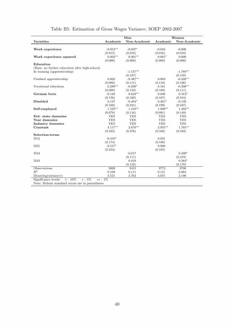
Table B5: Estimation of Gross Wages Variance, SOEP 2002-2007

Men WomenVariables Academic Non-Academic Academic Non-Academic

Work experience -0.053∗∗ -0.037∗ -0.016 -0.006(0.013) (0.016) (0.016) (0.016)

Work experience squared 0.002∗∗ 0.001∗∗ 0.001† 0.000(0.000) (0.000) (0.000) (0.000)

Education(Base: no further education after high-school)In training (apprenticeship) -1.557∗∗ -1.789∗∗

(0.187) (0.158)Finished apprenticeship 0.002 -0.487∗∗ 0.003 -0.328∗∗

(0.080) (0.111) (0.110) (0.106)Vocational education 0.288∗∗ -0.298∗ 0.161 -0.306∗∗

(0.099) (0.122) (0.109) (0.111)German born -0.129 0.624∗∗ 0.040 0.312†

(0.136) (0.160) (0.167) (0.164)Disabled 0.137 -0.494∗ 0.361† -0.139

(0.160) (0.221) (0.199) (0.247)Self-employed 1.525∗∗ 1.419∗∗ 1.899∗∗ 1.402∗∗

(0.078) (0.116) (0.091) (0.149)Fed. state dummies YES YES YES YESYear dummies YES YES YES YESIndustry dummies YES YES YES YESConstant 4.117∗∗ 2.678∗∗ 2.955∗∗ 1.785∗∗

(0.242) (0.276) (0.348) (0.349)Selection-termsM12 -0.410∗ 0.021

(0.174) (0.186)M21 -0.517∗ 0.068

(0.234) (0.185)M34 -0.017 0.499∗

(0.111) (0.219)M43 0.019 0.384∗

(0.122) (0.170)Observations 5800 3415 3773 3706R2 0.109 0.111 0.151 0.084Mean(log(variance)) 3.521 2.763 3.075 2.190Significance levels: † : 10% ∗ : 5% ∗∗ : 1%Note: Robust standard errors are in parentheses

40

Table B6: Transition to Tertiary Education: Full Results

γ = 1.02 γ = 1.05 γ = 1.08 γ = 1.10Coef. Coef. Coef. Coef.

Eligible for student aid -0.428∗ -0.431∗ -0.435∗ -0.437∗

(0.174) (0.175) (0.175) (0.174)Age when finished highschool 0.108 0.122 0.173 0.221

(1.627) (1.625) (1.625) (1.627)Age when finished highschool squared 0.008 0.007 0.006 0.005

(0.042) (0.042) (0.042) (0.042)Mother holds university degree 0.591∗∗ 0.593∗∗ 0.593∗∗ 0.592∗∗

(0.178) (0.178) (0.178) (0.178)Father holds university degree 0.127 0.127 0.128 0.129

(0.168) (0.168) (0.168) (0.168)Parental net income (in 1000 EUR) 0.021 0.021 0.021 0.021

(0.043) (0.043) (0.043) (0.043)At age 17 the highest degree intended wasUniversity degree 0.719∗∗ 0.727∗∗ 0.735∗∗ 0.742∗∗

(0.271) (0.271) (0.270) (0.269)n.a. 0.242 0.248 0.254 0.258

(0.308) (0.308) (0.307) (0.307)Respondent has one sibling -0.371∗ -0.369∗ -0.366∗ -0.363∗

(0.163) (0.163) (0.163) (0.162)Respondent has more than one sibling 0.138 0.139 0.143 0.146

(0.277) (0.277) (0.277) (0.277)Finished apprenticeship 0.653† 0.663† 0.646† 0.621†

(0.354) (0.357) (0.356) (0.354)School grades in German at age 17(Base: Good (2))n.a. 1.116 1.098 1.074 1.055

(1.050) (1.046) (1.041) (1.038)Very good (1) 1.596∗∗ 1.590∗∗ 1.583∗∗ 1.578∗∗

(0.464) (0.464) (0.465) (0.465)Satisfactory (3) -0.112 -0.113 -0.113 -0.114

(0.203) (0.203) (0.203) (0.203)Poor (4-6) -0.271 -0.269 -0.265 -0.260

(0.334) (0.334) (0.334) (0.334)School grades in math at age 17(Base: Good (2))n.a. -0.905 -0.885 -0.857 -0.836

(1.039) (1.035) (1.031) (1.028)Very good (1) 0.675∗ 0.666∗ 0.655∗ 0.647∗

(0.326) (0.326) (0.326) (0.326)Satisfactory (3) 0.179 0.183 0.187 0.190

(0.225) (0.225) (0.225) (0.225)Poor (4-6) -0.471† -0.463† -0.455† -0.449

(0.276) (0.276) (0.276) (0.276)Male -1.030∗∗ -0.985∗∗ -0.936∗∗ -0.908∗∗

(0.242) (0.242) (0.242) (0.243)Baseline hazard: time since high-school graduation(Base: up to one year)Two years -0.401 -0.419 -0.429 -0.432

(0.263) (0.264) (0.264) (0.264)Three years -0.040 -0.057 -0.063 -0.066

(0.347) (0.347) (0.348) (0.348)Four years 0.789∗ 0.775∗ 0.773∗ 0.770∗

(0.385) (0.384) (0.384) (0.384)Five years 0.272 0.265 0.277 0.287

(0.439) (0.438) (0.437) (0.437)Two years x male 2.311∗∗ 2.308∗∗ 2.307∗∗ 2.308∗∗

(0.367) (0.367) (0.367) (0.367)Three years x male 1.360∗∗ 1.327∗∗ 1.300∗∗ 1.289∗∗

(0.439) (0.440) (0.441) (0.442)Four years x male 0.897† 0.832† 0.776 0.748

(0.478) (0.478) (0.478) (0.478)Five years x male 1.817∗∗ 1.740∗∗ 1.667∗∗ 1.626∗∗

(0.517) (0.516) (0.515) (0.514)Regional dummies(Base: West)East 0.528∗ 0.458∗ 0.378† 0.324

Continued on next page...

41

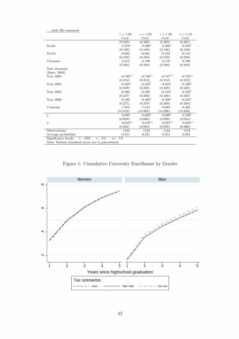
... table B6 continuedγ = 1.02 γ = 1.05 γ = 1.08 γ = 1.10

Coef. Coef. Coef. Coef.(0.209) (0.206) (0.203) (0.201)

South 0.378∗ 0.386∗ 0.392∗ 0.395∗

(0.189) (0.189) (0.188) (0.188)North -0.062 -0.081 -0.103 -0.118

(0.259) (0.259) (0.259) (0.259)Citystate 0.212 0.196 0.179 0.169

(0.394) (0.394) (0.394) (0.394)Year dummies(Base: 2002)Year 2003 -0.730∗∗ -0.740∗∗ -0.747∗∗ -0.752∗∗

(0.212) (0.212) (0.212) (0.212)Year 2004 -0.433† -0.433† -0.434† -0.436†

(0.229) (0.229) (0.228) (0.228)Year 2005 -0.380 -0.392 -0.410† -0.423†

(0.247) (0.246) (0.246) (0.245)Year 2006 -0.430 -0.466† -0.500† -0.523†

(0.271) (0.270) (0.269) (0.268)Constant -7.953 -7.814 -8.083 -8.405

(15.819) (15.802) (15.808) (15.826)

ρ 0.099 0.099† 0.099† 0.100†

(0.063) (0.060) (0.056) (0.054)α 0.010∗∗ 0.016∗∗ 0.023∗∗ 0.029∗∗

(0.002) (0.003) (0.005) (0.006)Observations 1144 1144 1144 1144Average probability 0.351 0.351 0.351 0.351Significance levels: † : 10% ∗ : 5% ∗∗ : 1%Note: Robust standard errors are in parentheses

Figure 1: Cumulative University Enrollment by Gender

.2.4

.6.8

1 2 3 4 5 1 2 3 4 5

Women Men

base high−high low−low

Tax scenarios:

Years since highschool graduation

42