Identifying Exporterâ€™s Relative Product Quality Variation from

Identifying Exporter’s Relative Product Quality Variation from ExportUnit Values Using Revealed Preference Analysis∗

Juan Carlos Hallak†

University of Michigan & NBER

Peter K. Schott‡

Yale School of Management & NBER

INCOMPLETE DRAFT

February 2005

Abstract

This paper develops a methodology for decomposing cross-country variation in export unit valuesinto quality versus real price components. The methodology is based on revealed preferences inan environment where consumers have a taste for variety. We derive conditions under which theunobserved export quality ratio of any two exporters is bounded by the observed Paasche andLaspeyres price indexes defined over their common exports to a third country. We then showthat price variation not associated with variation in export product quality can be identified usinginformation on countries’ trade balance, and introduce a technique for adjusting the bounds toincorporate this information. Finally, we use our methodology to estimate the evolution of U.S.trading parter export quality from 1974 to 2001.

Keywords: Import Prices; Export Quality; Revealed Preferences; Paasche; Laspeyres

JEL classification: F1; F2; F4

∗We thank Keith Chen, Alan Deardorff and Ben Polak for their generosity with comments and insight.†611 Tappan Street, Ann Arbor, MI 48109, tel : (734) 763-9619, fax : (734) 764-2769, email : hal-

[email protected]‡135 Prospect Street, New Haven, CT 06520, tel : (203) 436-4260, fax : (203) 432-6974, email : pe-

[email protected]

Identifying Relative Export Quality 2

1. Introduction

A growing body of empirical research suggests that variation in product quality is animportant determinant of international trade patterns and a crucial dimension for economicdevelopment.1 Failure to account for this variation can result in erroneous conclusions aboutboth the usefulness of trade theory and the effectiveness of trade policy. Unfortunately,reliable data on export product quality are unavailable for most countries, industries andyears. We address this need by developing a methodology to identify exporters’ unobservedexport quality from observed variation in readily available export unit values and quantities.

Export unit values vary considerably across countries even within narrowly defined prod-uct categories. It is often assumed that this variation is driven by vertical differentiationin quality or other hedonic attributes. Shirt varieties from Italy that are four times asexpensive as shirt varieties from China, for example, might be considered four times as“fashionable”. (We use the term “variety” to refer to one country’s particular exportwithin a product category; we use the terms “good” and “product” interchangeably to referto product categories. “Sectors” and “industries” are aggregations of product categories.)Similar assumptions are made in the study of intra-industry trade, where horizontal andvertical trade flows are differentiated according to whether unit value ratios are within oroutside a 0.85 to 1.15 interval, respectively.2 Estimates of countries’ “quality competitive-ness” are also often recovered from export unit values.3

Cross-country variation in export prices, however, may be influenced by other factors,in particular “pure” price variation induced by comparative advantage, i.e. variation inexporters’ relative production efficiency or factor costs. As a result, an ability to distinguishbetween quality and comparative advantage is critical.

Our methodology decomposes cross-country variation in export unit values within sec-

1Recent research suggests that export quality is influential in determining the direction of trade (Hallak2004), the skill premium in developing countries (Verhoogen 2004), and export success among firms (Brooks2003, Verhoogen 2004). Data aggregation that obscures cross-country variation in product quality alsohelps explain previous poor empirical support for the Heckscher-Ohlin model (Schott 2003, 2004). Withrespect to economic development, countries doubling their per worker GDP export 34% higher quantities at9% higher prices within a typical export category (Hummels and Klenow 2004).

2This rule of thumb is suggested by Abed-el-Rahman (1991). Aturupane et al. (1999), for example,find a positive association between vertical intra-industry trade and product differentiation, economies ofscale, the labor intensity of production and foreign direct investment. Aiginger (1997) proposes furtherdifferentiating vertical intra-industry trade flows according to whether they are accompanied by a tradesurplus or deficit.

3See, for example, Aiginger (OECD 1998), Verma (ICRIER 2002) and Ianchovichina et al. (IADB/WorldBank 2003).


tors into quality versus pure price components. The analysis extracts information abouteach country’s export quality from the full set of bilateral comparisons across trading part-ners. We show conditions under which the unobserved ratio of export quality between anytwo exporters is bounded by the observed Paasche and Laspeyres price indexes defined overtheir common exports to a third country. We assume that export quality is constant acrossproducts within a sector for each exporter.

The theoretical framework is based on revealed preferences in an environment whereconsumers have a taste for variety, and where products are not only vertically but also hor-izontally differentiated.4 In particular, a country that exports in a given product categorymay export an unobservable number of horizontally differentiated varieties in that category.This flexibility, while desirable as a feature of the theoretical framework, complicates theanalysis considerably because it introduces an additional factor besides quality that mayinfluence the relationship between export price and quantity. All else equal, countriesexporting a larger number of varieties will export larger quantities at any given price. Fail-ure to consider the influence of this greater number of varieties may result in the spuriousconclusion that these countries’ larger exported quantities are the result of higher productquality. Our methodology accounts for this potential influence explicitly.

A key aspect of our analysis is the use of “conditional expenditure functions”. Thesefunctions identify the minimum expenditure on a subset of varieties imported from one coun-try that is necessary to attain a certain level of utility, conditional on the actual quantitiesof varieties imported from that and other countries.

We link unobserved quality and observed export prices and quantities in two steps.First, we use revealed preference to show that the Paasche and Laspeyres price indexesare, respectively, smaller and greater than (unobserved) minimum conditional expenditurechanges that occur in response to price changes. Second, we demonstrate that the ex-porter quality ratio lies between these minimum conditional expenditure changes under theassumption of constant elasticity of substitution (CES) preferences. This yields the resultthat relative export quality is bounded by the Paasche and Laspeyres price indexes. Aconvenient property of this approach is that, even though it assumes CES preferences inthe second step, it does not require knowledge of the elasticity of substitution parameter.

The Paasche and Laspeyres indexes bound quality under a strong condition: a “pure”price index, which is a summary measure of comparative advantage, must be equal across

4A large body of theoretical and empirical research in international trade emphasizes the importance ofhorizontal differentiation in determining bilateral trade flows, the evolution of countries terms of trade, andexchange rates. Seminal theoretical contributions include Krugman (1980, 1981), Helpman and Krugman(1985) and Krugman (1989).


countries. Some form of this condition is implicit in usual inferences of quality from exportunit values. We interpret this condition as a requirement that every country has balancedtrade. While this assumption is plausible for a country’s aggregate trade, it may not be truefor trade in the particular sector for which export quality is being estimated. Fortunately,the theoretical framework developed in this paper permits relaxing this condition. We showthat, by exploiting additional information on countries’ trade flows (in particular, sectoraltrade balance) we can identify variation in “pure” price indexes. This variation is then usedto adjust the Paasche and Laspeyres bounds on quality.

Though substantively situated in international economics, this paper also contributesto the very large literature on index number theory. A key focus of that literature is theconstruction of price indexes that control for changes in product quality over time. Here, wehave a different aim: rather than measure quality changes in bundles of products purchasedover time, we seek to identify quality variation over simultaneously purchased bundles fromdifferent sources of supply.5 We also operate under different information constraints. Inparticular, we have no knowledge of export products’ underlying attributes, or the numberof horizontal varieties each exporter sells in each product category. As a result, we areunable to make use of standard strategies — such as hedonic pricing — that use additionalinformation on product characteristics to adjust price indexes for quality.6 Data constraintsalso prevent us from adopting the approach of the International Price Program of the U.S.Bureau of Labor Statistics, which constructs import and export price indexes by combiningsurvey data on firm prices with firms’ assessments about changes in their products’ qualityover time.7 Our methodology complements such efforts, however, because its use of widelyavailable trade data permits estimation of exporter quality across a broad range of countriesand products for which survey data may be unavailable or prohibitively expensive.

Another promising and related application of our methodology is the measurement ofnational accounts aggregates at internationally comparable prices. Current estimates of“real GDP”, such as the Penn World Tables, deflate nominal GDP using a purchasingpower parity (PPP) deflator based on final expenditure data. This measure of real GDPmay not be optimal for capturing changes in countries’ production over time. A recentcontribution to the literature suggests using a PPP deflator constructed from output prices

5Aw and Roberts (1986) and Feenstra (1988) identify quality upgrading over time — defined as an across-product shift from lower- to higher-priced exports — in response to quantitative trade restrictions. Inaddition to focusing on time-series changes, that conceptualization of quality change differs from ours inthat it does not take into account potential within-product changes in product quality.

6Feenstra (1995), for example, demonstrates how information on product attributes can be used toestablish bounds on the exact hedonic price index.

7See www.bls.gov/mxp/ for more detail.


rather than expenditure prices (Feenstra et al. 2004). This new deflator would includea terms-of-trade correction estimated from import and export price indexes based on unitvalues. An ability to net quality out of these indexes before performing the terms-of-tradecorrection would enhance their accuracy.

The remainder of the paper is structured as follows. Section 2 defines notation. Section3 outlines our framework. Section 4 implements our framework using U.S. import data.Section 5 concludes.

2. Definitions and Notation

Export product categories are indexed z = 1, ...,Ω.8 Countries are indexed k = 1, ..., C.A country is “active” in product z if it reports positive exports to the United States in thatcategory. Define nkz as the (unobserved) number of varieties of product z that countryk exports to the United States. We assume that all varieties of product z exported bycountry k are horizontally differentiated in the sense that preferences over them, as well astheir prices, are symmetric. As a result, each variety is consumed in the same quantity.Let pkz be the price of a typical variety of product z produced in country z, xkz be thequantity consumed per variety, λkz be the quality level, and ξkz be a demand shifter. Thetotal quantity of country k exports of product z to the United States is then qkz = nkzx

kz .

Categories z are grouped into sectors s = 1, ..., S. Let Is be the set of categories zin sector s, and Iks be the set of “active” categories in country k. In the data, s maycorrespond to one-digit SITC industries or some other level of aggregation. Let vectorps include the U.S. import prices of all active categories in sector s from all countries.9

Analogously, define vectors qs,ns,λs, and ξs. Finally, stack these vectors across sectors toform vectors p, q, n, λ, and ξ.

Since our methodology is based on comparing export prices (as measured by unit values)across pairs of U.S. trading partners, we need to develop additional notation specific tocountry pairs. Index the two countries in a pair of U.S. trading partners by c and d.Denote by Icds the set of active categories common to c and d in sector s. Similarly, Ic,−ds isthe set of products in which c is active but not d, Id,−cs is the set of products in which d isactive but not c, and U cd

s is the union of these two sets. Finally, ∅cds is the set of products

in which neither of the two countries is active. The set Is can then be partitioned into

8 In the data to which we apply our methodology, these categories correspond to seven-digit Tariff Systemof the United States (TSUSA) and ten-digit Harmonized System (HS) categories.

9Non-active categories could also be included in this vector; as we note in Section 3.3.2. below, we assumetheir prices, pkz , are infinite.


Icds , Ucds , and ∅cd

s . We can use Icds to break each of p and q into two components. First,

alternatively for each i = c, d, pis and qis include prices and quantities of exports by i in

products z ∈ Icds , respectively. The remaining parts of p and q are denoted by p−is andq−is . These vectors include categories z ∈ Icds exported by all countries other than i, andalso categories z /∈ Icds exported by all countries (including i).

3. Bounds on bilateral relative quality

In this section we demonstrate the assumptions required for estimating bounds on un-observable country export quality using observable export prices and quantities.

3.1. The Conditional Expenditure Function

For a country pair including countries c and d, define the conditional expenditure (orimport) function mc

s(pis,q

−cs ,n,λ, ξ,U) as the minimum U.S. expenditure on varieties ex-

ported by country c in categories z ∈ Icds required to attain utility level U , conditionalon q−cs ,n,λ, ξ, when import prices of those varieties are pis (per-variety consumption x isimplicitly defined by q and n). The conditional expenditure function is the solution to theproblem

minqcs

pisqcs s.t. U(qcs,q

−cs ,n,λ, ξ) = U, (1)

where U(.) is the representative consumer utility function for the U.S. This function canbe defined directly over categories z instead of over varieties j as a result of our symmetryassumptions.

By revealed preference, the minimum (conditional) import expenditure on productsproduced by c in categories z ∈ Icds , when import prices of those products are p

cs, is the

actual import value,

mcs(p

cs,q

−cs ,n,λ, ξ,U) = pcsq

cs. (2)

However, the minimum import expenditure when prices are pds rather than pcs is equal to

or lower than pdsqcs. This is because the expenditure p

dsq

cs is sufficient for attaining utility

U but qcs is not necessarily optimal given pds. Hence

mcs(p

ds,q

−cs ,n,λ, ξ,U) ≤ pdsqcs. (3)

Taking the ratio of (2) over (3), we obtain

∆mcs ≡

mcs(p

cs,q

−cs ,n,λ, ξ,U)

mcs(p

ds,q

−cs ,n,λ, ξ,U)

≥ pcsq

cs

pdsqcs

≡ ecds . (4)


The left hand side of (4), ∆mcs, captures the increase in minimum expenditure on country

c’s varieties (in categories z ∈ Icds ) that would be necessary to maintain utility U , if importprices of those varieties changed from pds to p

cs, conditional on holding constant the number

and characteristics (including quality) of these varieties, and the number, characteristicsand quantity consumed of all other goods. Note that the right hand side of (4) is a Paascheimport price index defined over the country pair’s common exports in sector s.

Similarly, we can focus on imports from country d to obtain

∆mds ≡

mds(p

cs,q

−ds ,n,λ, ξ,U)

mds(p

ds,q

−ds ,n,λ, ξ,U)

≤ pcsq

ds

pdsqds

≡ 1

edcs, (5)

where 1/edcs is a Laspeyres import price index defined over the country pair’s commonexports in industry s.

3.2. The Conditional Expenditure Function Assuming CES Preferences

Exploiting the information contained in ∆mcs and ∆m

ds in equations 4 and 5 requires

an assumption about preferences. Assume that consumers’ utility function has two tiers.The upper tier is separable into sectoral sub-utility indexes us, which are defined over thecharacteristics and quantity consumed of varieties in the sector. The constraint in problem(1) can then be rewritten as:

U(qcs,q−cs ,n,λ, ξ) = U [u1, ..., us(q

cs,q

−cs ,n,λs, ξs), ..., uS] = U (6)

As already defined, vector qcs includes the consumption of varieties produced in i in cate-gories z ∈ Icds , while vector q

−cs includes both the consumption of varieties produced in c in

categories z /∈ Icds and the consumption of varieties produced in all other countries in anycategory z ∈ Is. Since the arguments of all the sub-utility indexes for sectors other thans are held constant in problem (1), the value of those sub-utility indexes is also constant.Denote by U the set of all (constant) sub-utility levels in those sectors. Then, we canrewrite (6) as

us(qcs,q

−cs ,n,λs, ξs) = g(U,U) (7)

where g(.) results from inverting U(.).Assume that sub-utility us is a constant elasticity of substitution aggregator,

us =

"Xk

Xz∈Is

nkz

³ξzλ

ksx

kz

´α#1/αα (0, 1) (8)


In equation (8), the demand shifter ξz captures differences in consumer valuation of goodsthat belong to different categories (e.g. tables versus chairs). The demand shifter is assumedto be product-specific and constant across countries for the same category: ξkz = ξz,∀k =1, ..., C. Quality is also modeled as a demand shifter, but is allowed to vary across countriesand is assumed constant across categories in sector s: λkz = λks ,∀z Is. Since we focus onexpenditure (imports) only on varieties produced by c in categories z ∈ Icds , it is convenientto rewrite (8) as:

us =

⎡⎣Xz∈Icds

niz¡ξzλ

izx

iz

¢α+ u∗s

⎤⎦1/α (9)

whereu∗s =

Xz /∈Icds

niz¡ξzλ

izx

iz

¢α+Xk 6=i

Xz∈Is

nkz

³ξzλ

kzx

kz

´α.

Substituting (9) into (7), and after some algebra, we obtain⎡⎣Xz∈Icds

niz¡ξzλ

izx

iz

¢α⎤⎦1/α = [g(U,U)α − u∗s]1α = U.

We can then rewrite the problem that defines the conditional expenditure function as

minxcz

Xz∈Icds

nczpizx

cz s.t

⎡⎣Xz∈Icds

ncz (ξzλczx

cz)α

⎤⎦1/α = U.

This problem is now very simple, as the solution is the product between the well-knownideal price index for a CES — the cost of obtaining one unit of utility — and the target levelof utility,

mcs(p

is,q

−cs ,λ, ξ,U) =

⎡⎣Xz∈Icds

ncz¡epicz ¢1−σ

⎤⎦ 11−σ

U, (10)

where σ = 11−α is the elasticity of substitution and

epicz = pizξzλ

cs

, (11)


is the “pure” price of product z, which adjusts the observed price of z in country i with thecharacteristics of products in that category in country c.10 In other words, epicz indicates thepure price that a variety in category z produced in country c would command if its pricewere replaced by the price of varieties in the same category produced in country i. Forexample, epccz is the pure price of country c’s exports.

Using (10) and (11) for i = c, d, we can obtain an explicit expression for∆mcs in equation

(4):

∆mcs =

mcs(p

cs,q

−cs ,n,λ, ξ,U)

mcs(p

ds,q

−cs ,n,λ, ξ,U)

=

⎡⎢⎢⎣P

z∈Icdsncz (epccz )1−σP

z∈Icdsncz (epdcz )1−σ

⎤⎥⎥⎦1

1−σ

(12)

It is straightforward to show that epdcz = λdsλcsepddz and that epcdz = λcs

λdsepccz . Thus, taking logarithms

on both sides of (12) and combining that equation with (4), we have

ln ecds ≤ ln∆mcs = ln

λcsλds+ ln

⎡⎢⎢⎣P


z∈Icdsncz (epddz )1−σ

⎤⎥⎥⎦1

1−σ

. (13)

Analogously, imposing the CES structure on (5), we can obtain an explicit expression for∆md

s:

ln1

edcs≥ ln∆md

s = lnλcsλds+ ln

⎡⎢⎢⎣P

z∈Icdsndz (epccz )1−σP

z∈Icdsndz (epddz )1−σ

⎤⎥⎥⎦1

1−σ

. (14)

Equations (13) and (14) relate the implications of consumer minimization to cross-sectional Paasche and Laspeyres price indexes. Though ∆mc

s and ∆mds both capture the

change in minimum expenditure induced by changing prices from pcs to pds, their magnitudes

typically will be different as the number of varieties from each trading partner, ncz and ndz,are likely to vary. The fact that ∆mc

s is unlikely to equal ∆mds highlights an important

10We could alternatively define “pure” price as epicz =pizλcz, i.e. not including the demand shifter. This

definition would be more directly linked to the the idea of a quality-adjusted price. We follow the definitionin (11) only for notational simplicity, noting that this is merely a notational choice.


difference between the “conditional expenditure function” approach developed here and asimilar analysis performed in a competitive environment using (unconditional) expenditurefunctions.11 While the “conditional expenditure function” approach is consistent with adifferentiated-product environment, it requires restrictions on the relationship between thenumber of varieties and “pure” prices.

If the last term in (13) is negative and if the last term in (14) is positive, then unob-servable relative trading partner quality could be bounded by the observable Paasche andLaspeyres indexes noted above, i.e.,

ecds ≤ ∆mcs ≤

λcsλds≤ ∆md

s ≤1

edcs. (15)

We demonstrate the conditions necessary for this result after introducing additional notationin the next section.

3.3. Additional Notation

3.3.1. Defining a Trading Partner’s “Excess” Varieties

This section develops notation related to the number of varieties exported by eachcountry. These quantities are used to identify product categories in which a country exports“excess” (i.e., above-average) varieties.

Let Zs be the total number of product categories in sector s, Zks be the total number

of product categories in which country k is active, and Zcds be the total number of product

categories common to exporters c and d. Define the average number of varieties exportedby country k across product categories in sector s, nks , to be

nks ≡1

Zs

Xz∈Is

nkz ∀k = 1, ...C. (16)

Define the “k-normalized” multilateral average number of varieties across trading partnersin sector z to be

nkz ≡1

C

CXl=1

nlznk

nl∀k = 1, ...C.

Note that this normalization re-scales, for each trading partner k, the number of varietiesfrom other trading partners l into common, country-k units according to the ratio of average

11See, for example, Appendix 1 of Feenstra (2003).


varieties in s from k and l. As a result, averages based on different normalizing countriesare proportional,

nkz = nlznk

nl∀k = 1, ...C. (17)

For each pair of countries c and d, define the pair’s “normalized” average number ofvarieties in sector z to be

bncz ≡ 12µncz + ndz

nc

nd

¶and bndz ≡ 12

µndz + ncz

nd

nc

¶,

where the two averages alternately reflect the use of a different country in the pair to bethe normalizing country. Here, too, the averages are proportional,

bndz = bncz ndnc . (18)

Finally, for i = c, d, define eniz = niz−bniz to be i’s “bilateral excess varieties” in product zrelative to the country-pair average, and eeniz = bniz−niz to be the country pair’s “multilateralexcess varieties” in product z relative to the world average. These excess varieties possessthree convenient properties:

Xz∈Is

eniz = 0 (19)

Xz∈Is

eeniz = 0 (20)

encz = −bncbnd endz. (21)

The first and second properties indicate that across product categories within country i,both bilateral and multilateral excess varieties sum to zero. The third property reveals thattwo countries cannot both have positive bilateral excess varieties in the same category.12

12Equation (19) is straightforward to obtain using the definitions of eniz, bniz, and ni. Equation (20) usesthe fact that ncz = 2bncz − ndz

nc

nd.


3.3.2. Defining Trading Partners’ (Quality-) “Unadjusted” Bilateral Price Indexes

This section introduces aggregate price indexes defined over all of an exporter’s productsin a sector. Below, we associate variation in these indexes with comparative advantage.

Choose country b as numeraire, or “base” country. Let eP ks be a variety-weighted “pure”

price index defined over product categories in sector s:13

eP ks =

"Xz∈Is

nbz

³epkkz ´1−σ# 11−σ

, ∀k. (22)

Note that each price in this index is weighted by the “b-normalized” multilateral averagenumber of varieties in each sector, so that sectors with a higher number of varieties receivegreater weight.

The “pure” price index eP ks is an aggregator of quality-adjusted prices. We can similarly

define a (quality-) “unadjusted” price index, which aggregates over observed prices, to be

P ks =

"Xz∈Is

nbzξσ−1z

³pkkz

´1−σ# 11−σ

, ∀k. (23)

In contrast to (22), the “unadjusted” price index (23) aggregates over prices that are con-taminated by quality. The “unadjusted” price index can be easily decomposed into qualityand “pure” price components, P k

s = λcs eP ks .

Let ∆ eP cds = eP c

s / eP ds and ∆P

cds = P c

s /Pds be the ratios of a country pair’s pure and

unadjusted price indexes, respectively.14 A similar decomposition then follows for the“unadjusted” price index ratio, ∆P cd

s = λcsλds∆ eP cd

s .Finally, let the bilateral difference in two countries’ pure prices in product category z

relative to their countries’ pure price index be

∆epcdz =

ÃepcczeP cs

!1−σ−ÃepddzeP d

s

!1−σ. (24)

A positive ∆epcdz indicates that country c has a lower pure price of z (relative to its averagepure price) than country d. Such differences may arise due to comparative advantage, i.e.,variation in exporters’ relative production efficiency or factor costs.13The range of products spanned by this index can be restricted to country k´s active categories.

Since¡epkkz ¢1−σ = 0 for non-active categories - as epkkz is infinite - this alternative formulation is equivalent to

(22).14∆ eP cd

s and ∆P cds are invariant to the choice of base country used to normalize the average number of

varieties in each product category.


3.4. Main Result: Bounding Relative Quality

In this section we lay out a set of sufficient conditions for unobserved quality to bebounded by observable Paasche and Laspeyres price indexes.

Proposition 1 For any two countries c and d, (unobserved) relative export quality in sectors, λcs/λ

ds, is bounded by the observable Paasche and Laspeyres indexes

ln ecds ≤ lnλcsλds≤ 1

ln edcs

if:(i) “Bilateral excess varieties” are negatively correlated with bilateral differences in

“pure” relative prices:covIcds

³encz,∆epcdz ´ ≥ 0(ii) Country-pair “multilateral excess varieties” are uncorrelated with bilateral differ-

ences in “pure” relative prices:

covIs

³eencz,∆epcdz ´ = 0(iii) Countries c and d are “similarly active” in export product markets:

δcds = δdcs = 0

(iv) The “pure” aggregate price ratio is equal for both countries:

∆ eP cds = 1,

where covIj (x, y) ≡Pz∈Ij

(xz − x) (yz − y) ,

δcds =1

1− σln

⎡⎢⎢⎢⎣1−P

z∈Ucds

encz 1Zcds

Pz∈Icds

∆epcdz + Pz∈Ucd

s

bncz∆epcdzP

z∈Icdsncz

³epddzePds

´1−σ⎤⎥⎥⎥⎦ , (25)

and δdcs is defined symmetrically.


Proof. See Appendix A.Assumption i states that “bilateral excess varieties” are negatively correlated with dif-

ferences in “pure” relative prices. International trade models with product differentiationthat do not assume factor price equalization (e.g., Romalis 2004, Bernard et al. 2004) findthat the relative number of varieties between two countries in a given industry is a negativefunction of industry relative prices. It is possible to reformulate these models in termsof efficiency-adjusted variables. Thus reinterpreted, these models predict that the relativenumber of varieties is a negative function of their relative “pure” prices. Assumption iis based on these results. However, it requires a substantially weaker condition, as it onlyimposes a negative correlation between excess varieties and relative “pure” price differences.

Assumption ii imposes no correlation between the country-pair’s “multilateral excessvarieties” and bilateral differences in “pure” relative prices. This is not a strong assumption,as there is no obvious connection between the country pair’s “excess” varieties relative tothe world average and relative comparative advantage among countries within the pair.

The magnitude of the terms δcds and δdcs relates both to the extent to which countries cand d are active in the same categories and to which they are active in a similar number ofcategories. Assumption iii requires that these terms are zero. A sufficient condition thatimplies assumption iii is that the two countries are active in the same categories. In thatcase, the numerator in equation (25) is zero, as it sums over elements of U cd

s , which becomesan empty set. However, it is still possible that the numerator is zero even if U cd

s is non-empty.More generally, both δcds and δdcs will tend to become smaller (in absolute magnitude) asthe number of mismatched active categories (in the numerator of (25)) decreases relative tothe number of matched active categories (in the denominator of 25). Also, since ∆epcdz > 0

and encz > 0 for z ∈ Ic,−ds , and ∆epcdz < 0 and encz < 0 for z ∈ Id,−cs , these terms will tend tobecome smaller when the number of products in Ic,−ds is similar to those in Id,−cs .

The terms δcds and δdcs capture a wedge in the relationship between “pure” price indexesand “pure” prices for individual products. Conditional on the “pure” price index, eP k

s , the“pure” price of an individual category, epkkz , tends to be higher the larger is the number ofactive categories. This is clearly seen by inverting (22) when “pure” prices are symmetric.In that case,

epkkz =

⎛⎜⎜⎜⎝³ eP k

s

´1−σXz∈Iks

nbz

⎞⎟⎟⎟⎠1

1−σ

, (26)


where the denominator of this expression - and hence epkkz - increases with the number ofactive categories. When the value of the denominator is the same for both c and d (e.g.when the overlap between active categories in c and d is perfect), the denominator is thesame for both countries. In that case, differences in “pure” price indexes between countriesmap directly into differences in “pure” prices of individual categories. In contrast, whenthe value of the denominator is different for the two countries, an adjustment is required toinfer differences between them in “pure” prices at the product level (and hence quality asa residual) from information on “pure” price indexes, which we have by assumption iv.

Assumption iv imposes the equality of “pure” price indexes between c and d. Thisassumption can be interpreted as a trade balance restriction. A country’s comparative ad-vantage in a product manifests as a relatively low “pure” price in that product. eP k

s is anindex of pure prices. As such, it can be thought of as a summary measure of country k’scomparative advantage in sector s. The lower is eP k

s , for example, the more one might ex-pect country i to have an overall trade surplus in that sector. eP k

s is a good indicator of tradebalance because the particular form of the index (equation 22) is able to capture appropri-ately the relative influence of each product’s pure price on trade volumes. There are threereasons for this. First, products with higher demand shifters (ξz), which are more likely tobe influential in determining trade balance, are given more weight.15 Second, conditionalon observed prices, quality and demand shifters, product categories encompassing a greaternumber of varieties (bncz), which are also more likely to be influential in determining tradebalance, also receive higher weights. Finally, the elasticity of substitution, σ, also plays arole. When σ is high, low prices have greater influence in the index, and this matches theirrole in determining trade balance.

Further intuition for assumption iv can be derived from considering a country pair inwhich country c (e.g. Bangladesh) has lower observed prices in all common products insector s (e.g. Apparel). In that case, both the Paasche and Laspeyres indexes would besmaller than unity. The relatively low prices of country c in sector s could be due to thatcountry’s lower quality. But they could also reflect its comparative advantage in all of theproducts in that sector, i.e. its lower “pure” prices. Without further information, we cannotdistinguish between the two possibilities. Only in the special case in which “pure” priceindexes do not differ between countries, as postulated by assumption iv, do the Paascheand Laspeyres indexes bound relative quality.

Assumption iv is strong. While we expect a trade balance restriction to bind at theaggregate level (at least in the long run), persistent trade imbalances at the sectoral level are

15Recall that the pure price epccz embeds the effect of the demand shifter ξz. If this shifter were removedfrom epccz , the weight on product z in (22) would be bncz (ξz)σ−1, which is increasing in ξz.


certainly possible, as countries might have a long-run comparative advantage in particularsectors (e.g. Bangladesh in Apparel). Proposition (1) does not allow for these imbalances.Moreover, without assumption iv, relative quality between two countries could not be iden-tified: depending upon which country has the comparative advantage, and its strength,either country’s good might be of higher quality.16 We note that, despite its disturbingimplications, some form of assumption iv is implicit in all inferences about export qualityderived solely from the comparison of unit values.

Our framework accommodates relaxing assumption iv, rendering possible identificationof relative export quality even in the presence of “pure” price index differences acrosscountries. Relaxing assumption iv, the derivation of Proposition (1) yields

ln ecds − ln∆ eP cds ≤ ln∆λcds ≤ − ln edcs − ln∆ eP cd

s . (27)

where ln∆λcds = lnλcs/λds . This equation indicates that relative quality can be identified

only when variation in “pure” prices is taken into account. If this is not done, then it canbe easily seen using ln∆P cd

s = ln∆ eP cds + ln∆λcds that the Paasche and Laspeyres indexes

do not bound relative quality but the (unobserved) “unadjusted” price index ratio

ln ecds ≤ ln∆P cds ≤ − ln edcs . (28)

As discussed above, information about countries’ sectoral trade balances can be exploitedto identify cross-country variation in “pure” prices. Here, we formalize the connection be-tween countries’ “pure” price index and their trade balance via a modification of assumptioniv,

Assumption iv0 : ln∆ eP cds = γ

³T cs /Y

c − T ds /Y

d´,

where T is/Y

i, i = c, d is country i’s trade balance (i.e., net exports) to GDP ratio in sectors.17 Since trade balances are observable, substituting assumption iv into (27) reveals thatknowledge of γ permits identification of relative export quality from observables,

ln ecds − γ∆Bcds ≤ ln∆λcds ≤ − ln edcs − γ∆Bcd

s , (29)

where ∆Bcds =

¡T cs /Y

c − T ds /Y

d¢.

16On the on hand, country d´s comparative advantage could be so strong that its observed lower pricesmask a substantially higher relative quality. On the other hand, the quality dominance of country c mightbe understated if all of its pure prices are relatively lower than those of country d.17Assumption iv0 implicitly defines eP k

s = ePs exp ¡γ ¡T ks /Y

k¢¢, where ePs is common across countries.


The next section discusses an estimation strategy for identifying relative export qualitybased on Proposition 1. Before concluding this section, we note that a convenient advantageof our approach is that, even though CES preferences are assumed to derive the minimumexpenditure functions, the bounds do not depend on the specific value that the substitutionparameter σ might take. Therefore, neither knowledge nor estimates of the value of thisparameter is required.

4. Estimating U.S. Trading Partners’ Relative Export Quality

In this section we use the bounds identified in Proposition 1 to estimate a ranking of theUnited States’ top 50 trading partners’ export quality over time. We begin by outliningour estimation strategy. We then describe our dataset and the results of implementing ourmethodology upon it.

4.1. Estimation Strategy

Our estimation proceeds in two stages. In the first stage we use data on export unit val-ues and quantities to estimate each country’s “unadjusted” price index relative to numeraire

country b, \ln∆P kbs , or more succinctly,

cP ks .18 In the second stage, this “unadjusted” price

is decomposed into pure-price and quality components via estimation of γ.For C trading partners, estimation of C − 1 “unadjusted” price indexes cP k

s requireschoosing the set of P k

s that satisfies the C(C − 1) pairs of inequalities in (28). To do that,we assume that the true Paasche and Laspeyres price ratios are observed with error.19

Denote the “true” and observed Paasche and Laspeyres indexes by e∗cds and 1/e∗dcs , andecds and 1/edcs , respectively. Then, ln ecds = ln e∗cds + ηcds and ln edcs = ln e∗dcs + ηdcs , whereηcds ∼ N(0, σ/wcd

s ) and ηdcs ∼ N(0, σ/wcds ) are assumed independent of each other and of

error terms for other bilateral pairs, and wcds is a weight.20 In the results presented below,

we set wcds equal to the square root of the number of active categories countries c and d have

in common relative to the minimum number of common categories in each year. Satisfying

18The choice of numeraire country is made without loss of generality.19For information on the extent of measurement error in the import unit values, see General Accounting

Office (1995).20Some error terms are mechanically correlated, as they are constructed from the same information on

export value and quantity. This is more strongly so for ηcds and ηdcs . While we are considering the feasibilityof allowing for the implied correlation between error terms, at this stage we are performing the estimationunder the assumption that they are independent.


the inequality constraints then implies that

ln∆P cds ≥ ln e∗cds =⇒ ηcds ≥ ln ecds − ln∆P cd

s

ln∆P cds ≤ − ln e∗dcs =⇒ ηdcs ≤ ln∆P cd

s − ln edcs . (30)

The first stage of the estimation strategy involves finding the set of cP ks (for every k 6= b)

and bσ that maximizes the likelihood that the “true” bounds contain all “unadjusted” priceindex ratios. This implies maximizing the sum of log-likelihood functions of the form

lcds = lnΦ

µln∆P cd

s − ln ecdsσ/wcd

s

¶+ lnΦ

µln∆P cd

s − ln edcsσ/wcd

s

¶(31)

over C(C − 1) country pairs, where Φ(·) is the standard normal cumulative distributionfunction. In the results presented below, we use Germany as the numeraire country, b =DEU .

The second stage of our estimation yields an estimate of γ that can be used to decomposethe first stage estimates of the unadjusted price indexes, cP k

s , into pure-price and quality

components. This estimation relies on variation in cP ks over time. Express the path of

country k’s quality relative to the numeraire country over time as a quadratic trend plus adisturbance,

ln∆λkbst = ln∆λkbs + αkb1 t+ αkb2 t

2 + εkbst , (32)

where t indexes years. Since a country’ unadjusted price index is the product of its pureprice index and export quality, P k

s = eP ks λ

ks , it can be divided by a similar expression for

the numeraire country. Taking logs of these expressions and incorporating trade balanceassumption iv0 yields

ln\∆P kbst = γ∆Bkb

st + αk0 ln∆λkbs + αk1t+ αk2t

2 + εkst. (33)

If the disturbances to the left hand side variable were uncorrelated with the regressors, wecould estimate (33) by OLS. However, such orthogonality is unlikely. Suppose that thereis a deviation of quality above the trend in a particular year (εkst > 0). This deviation maybe accompanied by an increase in prices that leaves the “pure” price index - and hencethe trade balance - unchanged. However, the increase in quality may also decrease “pure”prices, in which case the error term will be correlated with the trade balance. To dealwith this endogeneity problem, we use two instruments: the real exchange rate and thenon-manufacturing trade balance.


4.2. Data

Product-level U.S. import data available from the U.S. Census and compiled by Feenstraet al. (2002) record the customs value of all U.S. imports by source country from 1972 to2001. Imports are recorded according to thousands of finely detailed seven-digit TariffSystem of the United States (TSUSA) categories (1974 to 1988) and ten-digit HarmonizedSystem (HS) categories (1989 to 2001). Here, we focus exclusively on manufacturingproducts (i.e., products in SITC aggregates 5 through 8).21

The product-level trade data include information on both quantity and value for manygoods and countries, rendering possible the calculation of product unit values. We computethe unit value, or “price”, of product z from country c, pcz, by dividing import value (v

cz) by

import quantity (qcz), pcz = vcz/q

cz.22 Examples of the units employed to classify products

include dozens of shirts in apparel, square meters of carpet in textiles and pounds of folicacid in chemicals.

Product-level trade data are noisy due to within-product category heterogeneity as wellas the measurement error noted above. We therefore trim the data along two dimensionsbefore computing Paasche and Laspeyres indexes. The first trim involves dropping country-year-product observations with value less than $10,000 or quantity equal to 1. The secondtrim eliminates country-pair-year-product observations when the relative quantity or therelative price of the country-pair-product is either below the 1st percentile or above the99th percentile of all country-pair-product observations in that year. The first trim getsrid of unusual and apparently unrealistic imports while the second trim discards unreliablecountry comparisons.23

Data on countries trade balance to GDP ratios at the sector level are constructed bymerging nominal dollar-denominated trade flow and GDP data available in the Feenstraet al. (2004) World Trade Flows database and the World Bank’s Development Indicatorsdatabase, respectively. Estimates of countries real exchange rates are derived from theversion 6.1 of the Penn World Tables.24

21Use of U.S. trade data to compare countries assumes that countries’ exports to the U.S. accuratelyreflect the prices they would receive in alternate markets.22Availability of unit values ranges from 77 percent of product-country observations in 1972 to 84 percent

of observations in 2001.23We are currently refining this trimming methodology.24A country’s real exchange rate is found by dividing its purchasing-power-parity relative to the United

States (PPP) into its local currency per U.S. dollar exchange rate (XRAT).


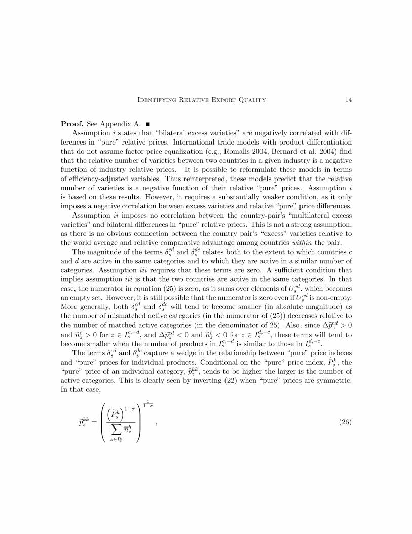
4.3. Estimation Results

Table 1 summarizes the results of the first stage maximum likelihood results. The loglikelihood and point estimates for bσ are reported for each year. The log likelihood declineswith time while bσ rises.25 Table 1 also displays the average number of common productsacross country pairs in each year. The maximum number of products in common rangesfrom 1340 in 1974 to 4737 in 2001.

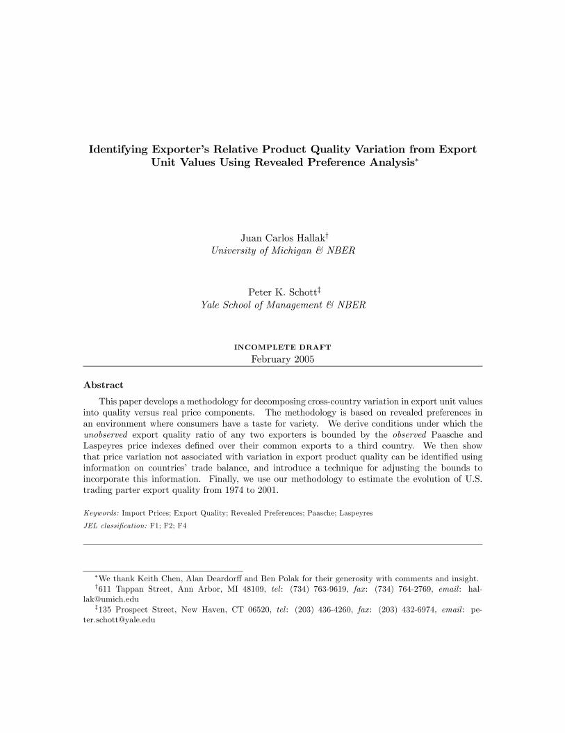
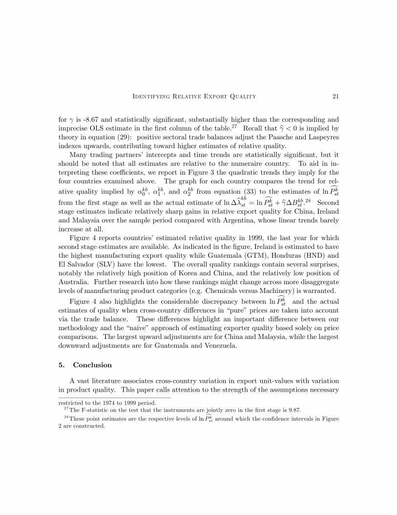
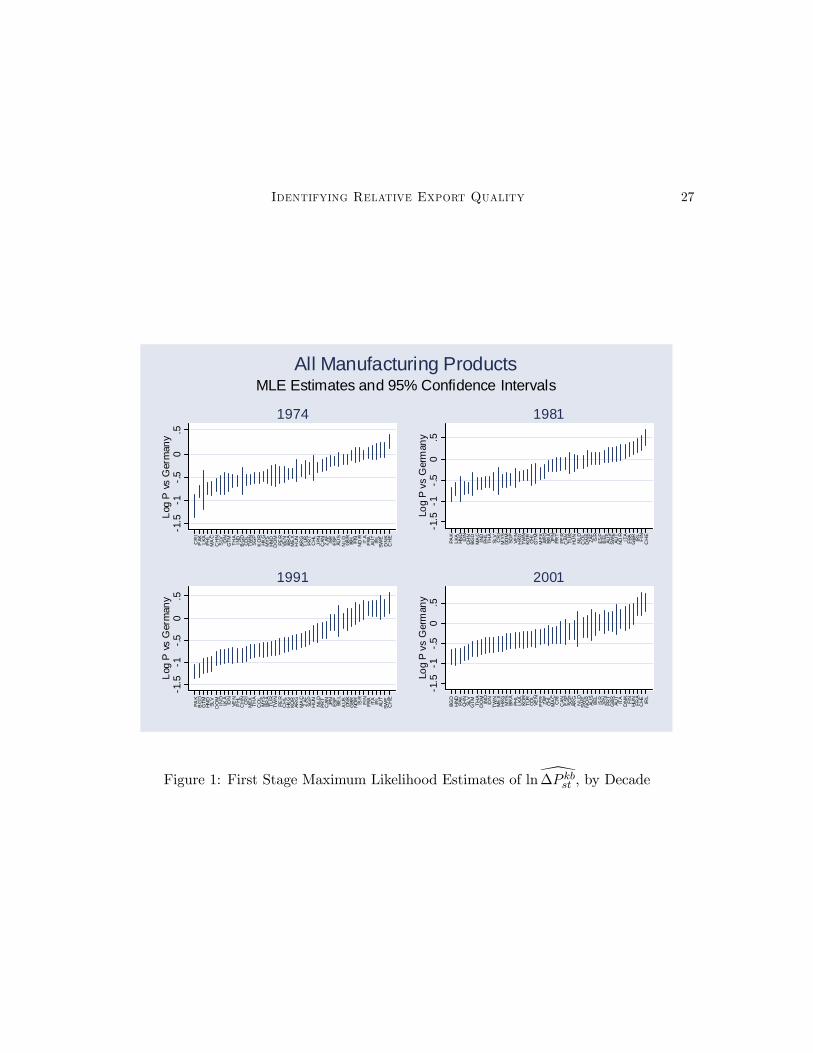
Figure 1 reports first stage estimates of lndP kbst for each trading partner along with their

associated 95 percent confidence intervals for four years, 1974, 1981, 1991 and 2001. Theseresults, at roughly ten year intervals, are representative of the variation observed more gen-erally in the estimates over time, and we report just these four years to conserve space. Thehorizontal axis sorts countries from low to high while the vertical axis reports each coun-

try’s ln cP kst relative to Germany, where lnP

DEUst = 0. The ordering of countries generally

accords with level of development, with higher-income countries generally having relativelyhigher unadjusted price indexes than lower-income developing countries. Pakistan (PAK)is among the lowest ranked countries in every year, with unadjusted prices roughly halfthose of Germany, while Switzerland (CHE) is among the highest. Somewhat surprisingly,

Ireland (IRL) is relatively highly ranked in all years, with ln\P IRLst significantly above the

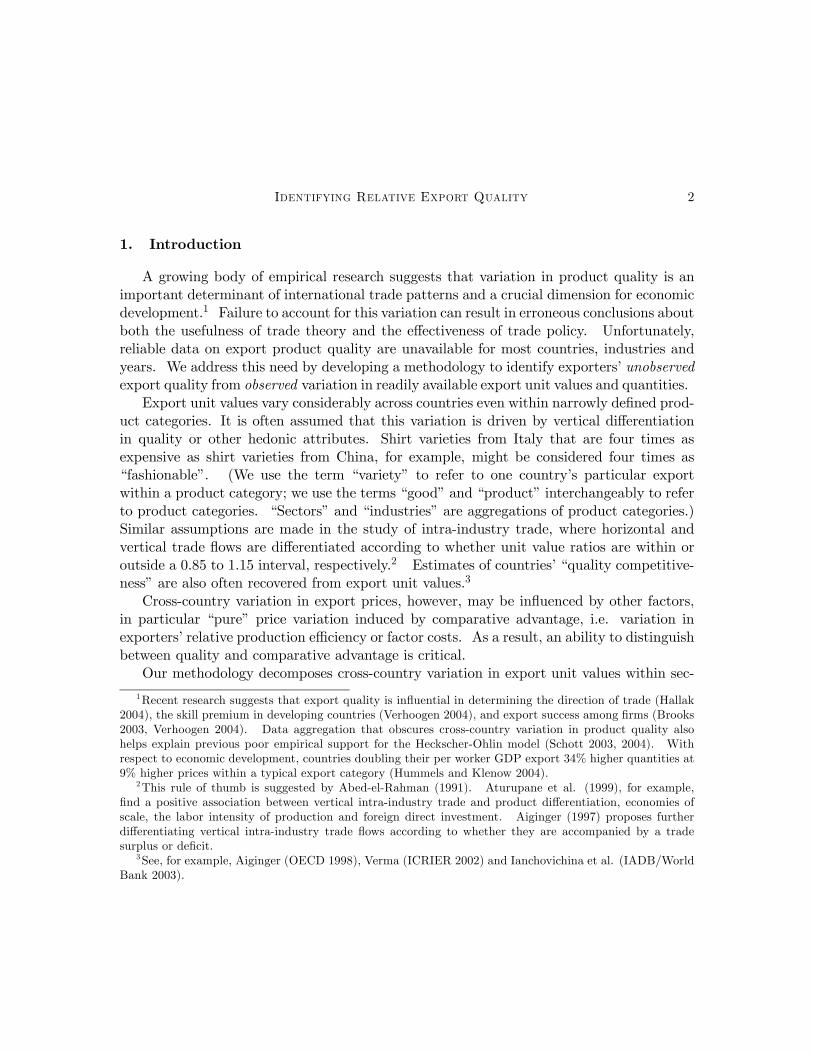
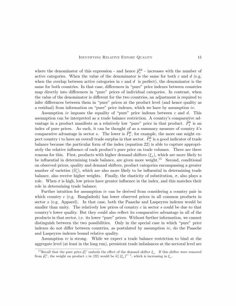
base country Germany in the last three years.Figure 2 provides an alternate view of the first stage results by tracing four countries’

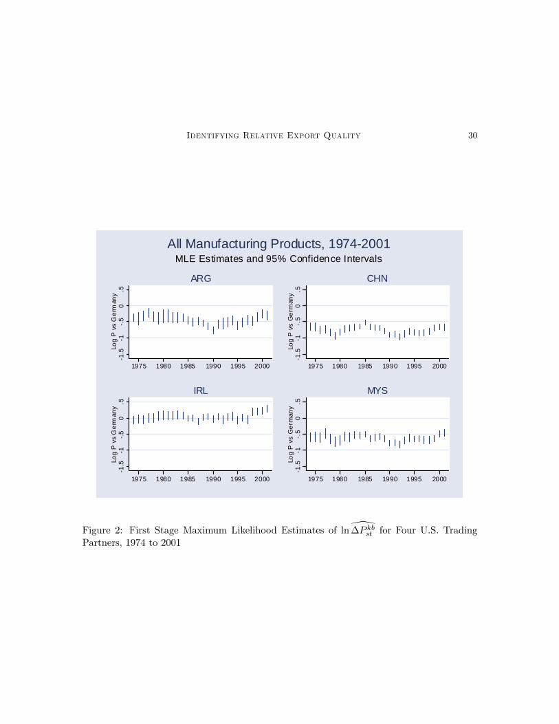
ln cP kst across the entire sample period. The four countries are Argentina (ARG), China

(CHN), Ireland (IRL), and Malaysia (MYS). Estimated unadjusted price indexes are rela-tively high for Ireland and relatively low for Argentina, China and Malaysia. All countries

exhibit cycles in their ln cP kst over time. These cycles are induced by various factors, in-

cluding movement in countries’ manufacturing trade balances as well as movement in theunadjusted price index of the numeraire base country. As is clear from equation (27), a

generally rising or falling trend in ln cP kst over time cannot be attributed to quality until

variation in pure prices ln eP kst, are netted out.

Tables 2 and 3 report the second-stage 2SLS estimates of γ from equation (33), where thereal exchange rate and the non-manufacturing trade balance are used to instrument for themanufacturing trade balance.26 As noted in Table 2, the instrumental variables estimate

25Recall that observations are weighted by 1/wcds , the square root of the number of products in which

countries c and d are active. As indicated in Table 1, this overlap — as well as the number of productcategories — increases with time.26Results for the first-stage of the 2SLS estimation are omitted to conserve space. Real exchange rate

data from the Penn World Tables is not availble after 1999. As a result, the second stage estimation is


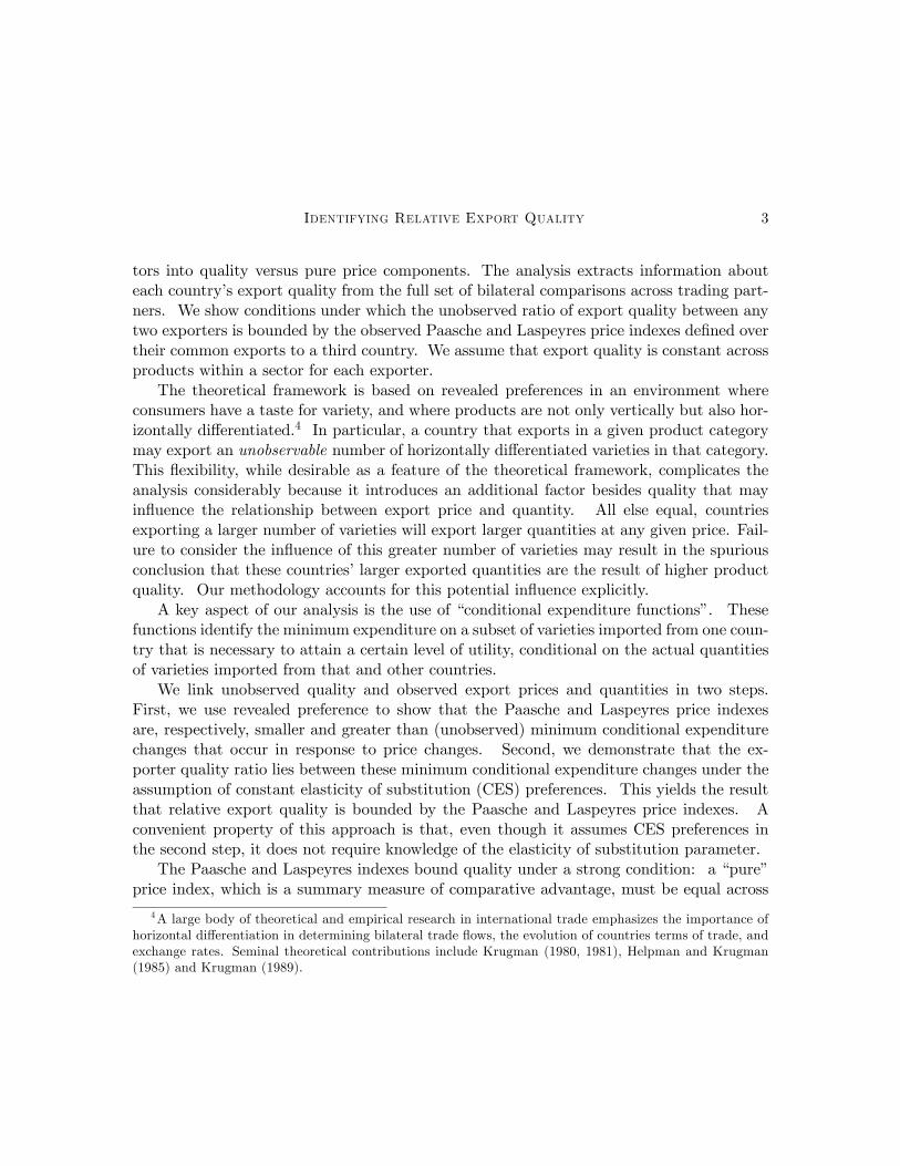
for γ is -8.67 and statistically significant, substantially higher than the corresponding andimprecise OLS estimate in the first column of the table.27 Recall that bγ < 0 is implied bytheory in equation (29): positive sectoral trade balances adjust the Paasche and Laspeyresindexes upwards, contributing toward higher estimates of relative quality.

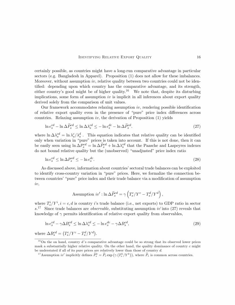
Many trading partners’ intercepts and time trends are statistically significant, but itshould be noted that all estimates are relative to the numeraire country. To aid in in-terpreting these coefficients, we report in Figure 3 the quadratic trends they imply for thefour countries examined above. The graph for each country compares the trend for rel-

ative quality implied by αkb0 , αkb1 , and αkb2 from equation (33) to the estimates of ln cP k

st

from the first stage as well as the actual estimate of ln∆bλkbst = ln cP kst + bγ∆Bkb

st .28 Second

stage estimates indicate relatively sharp gains in relative export quality for China, Irelandand Malaysia over the sample period compared with Argentina, whose linear trends barelyincrease at all.

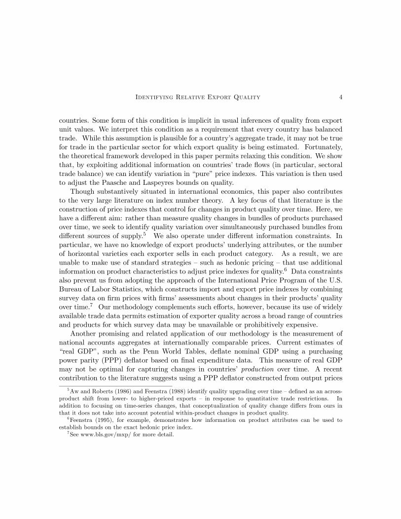
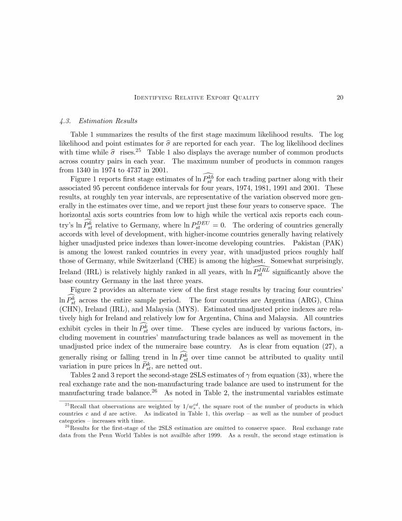
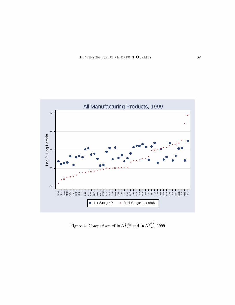
Figure 4 reports countries’ estimated relative quality in 1999, the last year for whichsecond stage estimates are available. As indicated in the figure, Ireland is estimated to havethe highest manufacturing export quality while Guatemala (GTM), Honduras (HND) andEl Salvador (SLV) have the lowest. The overall quality rankings contain several surprises,notably the relatively high position of Korea and China, and the relatively low position ofAustralia. Further research into how these rankings might change across more disaggregatelevels of manufacturing product categories (e.g. Chemicals versus Machinery) is warranted.

Figure 4 also highlights the considerable discrepancy between ln cP kst and the actual

estimates of quality when cross-country differences in “pure” prices are taken into accountvia the trade balance. These differences highlight an important difference between ourmethodology and the “naive” approach of estimating exporter quality based solely on pricecomparisons. The largest upward adjustments are for China and Malaysia, while the largestdownward adjustments are for Guatemala and Venezuela.

5. Conclusion

A vast literature associates cross-country variation in export unit-values with variationin product quality. This paper calls attention to the strength of the assumptions necessary

restricted to the 1974 to 1999 period.27The F-statistic on the test that the instruments are jointly zero in the first stage is 9.87.28These point estimates are the respective levels of ln cP k

st around which the confidence intervals in Figure2 are constructed.


to justify this approach and develops a methodology for exploiting information on countries’sectoral trade balance to identify pure price variation not associated with quality.


6. References

References

Abed-el-Rahman, K., 1991. Firms’ Competitive and National Comparative Advantages asJoint Determinants of Trade Composition. Weltwirtschaftliches Archiv, 127:83-97.

Aiginger, Karl, 1998. Unit Values to Signal the Quality Position of CEECs. In The Com-petitiveness of Transition Economies. OECD Proceedings, 1998(10):1-234.

Aiginger, Karl, 1997. The Use of Unit Values to Discriminate Between Price and QualityCompetition. Cambridge Journal of Economics, 21(5):571-592.

Aturupane, Chonira, Simeon Djankov and Bernard Hoekman, 1999. Horizontal and VerticalIntra-Industry Trade Between Eastern Europe and the EU. Weltwirtschaftliches Archiv,135(1):62-81.

Aw, Bee Yan and Mark J. Roberts, 1986. Measuring Quality Change in Quota-ConstrainedImport Markets. Journal of International Economics, 21(1): 45-60.

Bernard, Andrew B., Eaton, Jonathan, Jensen, J. Bradford and Samuel S. Kortum,2003. Plants and Productivity in International Trade. American Economic Review, 93(4):1268-1290.

Bernard, Andrew B., Stephen Redding and Peter K. Schott, 2004. Heterogenous Firms andComparative Advantage. NBER Working Paper 10668.

Brooks, Eileen, 2003. Why Don’t Firms Export More? Product Quality and ColombianPlants. UC Santa Cruz, mimeo.

Feenstra, Robert C., 1988. Quality Change Under Trade Restraints in Japanese Autos.Quarterly Journal of Economics, 103:131-146.

Feenstra, Robert C., 1995. Exact Hedonic Price Indexes. Review of Economics and Sta-tistics, 77:634-653.

Feenstra, Robert C., 2004. Advanced International Trade, Princeton University Press,Princeton, NJ.

Feenstra, Robert C., John Romalis and Peter K. Schott, 2002. U.S. Imports, Exports, andTariff Data, 1989-2001, NBER Working Paper 9387.


Feenstra, Robert C, Alan Heston, Marcel Timmer and Haiyan Deng, 2004. EstimatingReal Production and Expenditures Across Nations: A Proposal for Improving ExistingPractice. UC Davis, mimeo.

General Accounting Office, 1995. US Imports: Unit Values Vary Widely for IdenticallyClassified Commodities. Report GAO/GGD-95-90.

Hallak, Juan C., 2004. Product Quality, Linder and the Direction of Trade. NBERWorkingPaper 10877.

Helpman, Elhanan and Paul Krugman, 1985. Market Structure and Foreign Trade: In-creasing Returns, Imperfect Competition and the International Economy, MIT Press,Cambridge, MA.

Hummels, David and Peter Klenow, 2004. The Variety and Quality of a Nation’s Exports.Forthcoming in American Economic Review.

Ianchovichina, Elena, Sethaput Suthiwart-Narueput and Min Zhao, 2003. Regional Impactof China’s WTO Accession. In Krumm, Kathie and Homi Kharas (eds), East Asia Inte-grates: A Trade Policy Agenda for Shared Growth (Washington DC: The InternationalBank for Reconstruction and Development / The World Bank).

Krugman, Paul R., 1979. Increasing Returns, Monopolistic Competition, and InternationalTrade. Journal of International Economics IX:469-479.

Krugman, Paul R., 1980. Scale Economies, Product Differentiation and the Pattern ofTrade. American Economic Review LXX:950-959.

Krugman, Paul R., 1989. Differences in Income Elasticities and Trends in Real ExchangeRates. European Economic Review 33:1055-85.

Romalis, John, 2004. Factor Proportions and the Structure of Commodity Trade. AmericanEconomic Review, 94: 67-97.

Schott, Peter K, 2003. One Size Fits All? Heckscher-Ohlin Specialization in Global Pro-duction. American Economic Review, 93: 686-708.

Schott, Peter K, 2004. Across-Product versus Within-Product Specialization in Interna-tional Trade. Quarterly Journal of Economics, 119(2): 647-678.


Verhoogen, Eric, 2004. Trade, Quality Upgrading, and Wage Inequality in the MexicanManufacturing Sector: Theory and Evidence from an Exchange-Rate Shock. UC Berke-ley, mimeo.

Verma, Samar, 2002. Export Competitiveness of Indian Textile and Garment Industry.Indian Council for Research on International Economic Relations, Working Paper 94.

7. Appendix A: Proof of Proposition 1

Proof. We use extensively the fact thatPz∈Ij

xzyz = covIj (x, y) + Zjxy.

We first need to show that ln ecds − δcds ≤ lnλcsλds+ ln∆ eP cd

s . As a starting point, we show

thatP

z∈Icdsncz∆epcdz ≥ − P

z∈Ucds

encz 1Zcds

Pz∈Icds

∆epcdz − Pz∈Ucd

s

bncz∆epcdz :

Xz∈Icds

ncz∆epcdz =Xz∈Icds

encz∆epcdz +Xz∈Is

bncz∆epcdz − Xz∈Ucd

s

bncz∆epcdz =

= Zcds covIcds

³encz,∆epcdz ´+ Xz∈Ucd

s

encz 1

Zcds

Xz∈Icds

∆epcdz + (34)

covIs

³eencz,∆epcdz ´+Xz∈Is

ncz∆epcdz − Xz∈Ucd

s

bncz∆epcdz≥ −

Xz∈Ucd

s

encz 1

Zcds

Xz∈Icds

∆epcdz − Xz∈Ucd

s

bncz∆epcdzThe first equality uses ncz = encz + bncz and P

z∈Icdsncz∆epcdz =

Pz∈Is

bncz∆epcdz − Pz∈Ucd

s

bncz∆epcdz . Thesecond equality uses the definition of covariance and bncz = eencz + ncz. The inequality usesassumptions i and ii, and also the definition of eP k

s in (22), which implies thatPz∈Is

ncz∆epcdz =

0.Decomposing ∆epcdz according to its definition in (24), taking the second term to the

right hand side, and dividing both sides by this term, we obtainPz∈Icds

ncz

³ epcczeP cs

´1−σP

z∈Icdsncz

³epddzePds

´1−σ ≥ 1− δ0cds (35)


where δ0cds ≡

Pz∈Ucds

encz 1

Zcds

Pz∈Icds

∆epcdz + Pz∈Ucds

bncz∆epcdzP

z∈Icds

ncz

µ epddzePds¶1−σ .

Elevating both sides of (35) to the (negative) exponent of 1− σ, and performing basicalgebra manipulation:

ln

⎛⎜⎜⎝P


z∈Icdsncz (epddz )1−σ

⎞⎟⎟⎠1

1−σ

≤ ln∆ eP cds + δcds (36)

where δcds ≡ 11−σ ln(1− δ0cds ). Then, combining (13) with (36), we obtain

ln ecds − δcds ≤ lnλcsλds+ ln∆ eP cd

s . (37)

Symmetrically, it can be shown that ln λcsλds+ln∆ eP cd

s ≤ 1ln edcs −δdcs

. Therefore, the productof relative quality and relative pure price indexes is bounded by the Laspeyres and Paascheindexes, respectively adjusted by δcds and δ

dcs . Since assumption iii imposes that these terms

are zero, we obtain

ln ecds ≤ lnλcsλds+ ln∆ eP cd

s ≤1

ln edcs(38)

Finally, assumption iv reduces this expression to bound on relative quality

ln ecds ≤ lnλcsλds≤ 1

ln edcs


-1.5

-1-.5

0.5

Log

P v

s G

erm

any

CR

I P

AK L

KA P

HL

MA

C C

HN

SLV

IDN

GTM

TH

A IN

D B

GD

CO

L T

WN

SG

P K

OR

HK

G M

YS H

ND

DO

M P

ER

VE

N B

RA

ME

X H

UN A

RG

TUR

PR

T C

HL J

PN C

AN Z

AF IS

R E

SP A

US

NLD

GB

R B

EL F

IN N

OR

ITA

FRA

AU

T IR

L S

WE

DN

K C

HE

1974-1

.5-1

-.50

.5Lo

g P

vs

Ger

man

y

PA

K L

KA H

ND

IDN

CH

N B

GD

MA

C IN

D P

HL

TH

A S

LV CR

I M

YS D

OM

SG

P V

EN

HKG

TW

N K

OR

CH

L G

TM M

EX A

RG

BR

A J

PN

PR

T P

ER

CAN

TU

R H

UN

NLD

CO

L D

NK

ZAF

ISR

ES

P B

EL A

US

SW

E A

UT

NO

R IT

A F

RA G

BR IRL

FIN

CH

E

1981

-1.5

-1-.5

0.5

Log

P v

s G

erm

any

PA

K B

GD

GTM

HN

D S

LV D

OM

IND

LK

A ID

N V

EN

PHL

CH

N C

RI

MEX

TH

A C

OL

MYS

BR

A T

UR

TW

N P

ER

CH

L H

KG

KO

R A

RG

MA

C Z

AF S

GP

HUN

NLD

PR

T C

AN J

PN E

SP B

EL

AUS

DN

K G

BR N

OR

ISR

FIN

FRA IT

A IR

L A

UT

SW

E C

HE

1991

-1.5

-1-.5

0.5

Log

P v

s G

erm

any

BG

D H

ND P

AK C

HN

SLV

GTM TH

A D

OM

IND

IDN

TW

N M

EX

HKG

MYS

BR

A P

HL

LKA

KO

R T

UR C

OL

VE

N P

ER Z

AF C

HL

MA

C C

RI C

AN E

SP S

GP

AR

G N

LD S

WE

NO

R A

US

BEL

ISR

JPN

PR

T G

BR A

UT

ITA

DN

K F

IN H

UN

FR

A C

HE IRL

2001

MLE Estimates and 95% Confidence IntervalsAll Manufacturing Products

Figure 1: First Stage Maximum Likelihood Estimates of ln\∆P kbst , by Decade


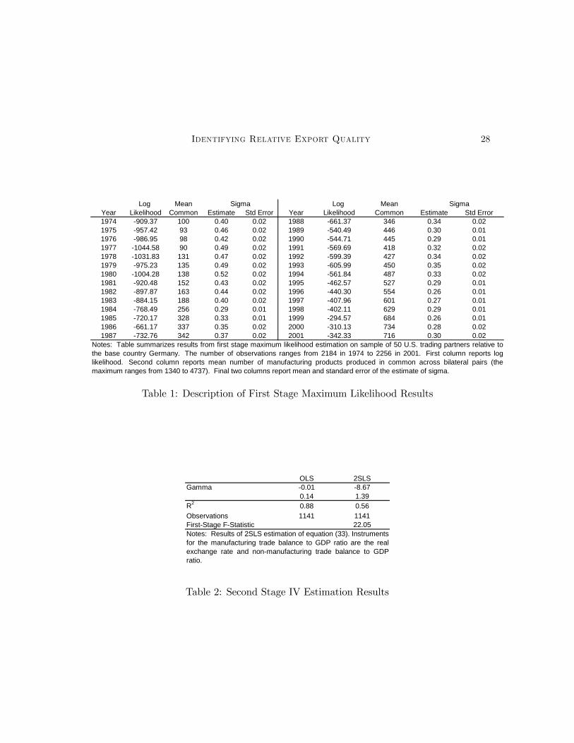
Log Mean Log MeanYear Likelihood Common Estimate Std Error Year Likelihood Common Estimate Std Error1974 -909.37 100 0.40 0.02 1988 -661.37 346 0.34 0.021975 -957.42 93 0.46 0.02 1989 -540.49 446 0.30 0.011976 -986.95 98 0.42 0.02 1990 -544.71 445 0.29 0.011977 -1044.58 90 0.49 0.02 1991 -569.69 418 0.32 0.021978 -1031.83 131 0.47 0.02 1992 -599.39 427 0.34 0.021979 -975.23 135 0.49 0.02 1993 -605.99 450 0.35 0.021980 -1004.28 138 0.52 0.02 1994 -561.84 487 0.33 0.021981 -920.48 152 0.43 0.02 1995 -462.57 527 0.29 0.011982 -897.87 163 0.44 0.02 1996 -440.30 554 0.26 0.011983 -884.15 188 0.40 0.02 1997 -407.96 601 0.27 0.011984 -768.49 256 0.29 0.01 1998 -402.11 629 0.29 0.011985 -720.17 328 0.33 0.01 1999 -294.57 684 0.26 0.011986 -661.17 337 0.35 0.02 2000 -310.13 734 0.28 0.021987 -732.76 342 0.37 0.02 2001 -342.33 716 0.30 0.02

Sigma Sigma

Notes: Table summarizes results from first stage maximum likelihood estimation on sample of 50 U.S. trading partners relative tothe base country Germany. The number of observations ranges from 2184 in 1974 to 2256 in 2001. First column reports loglikelihood. Second column reports mean number of manufacturing products produced in common across bilateral pairs (themaximum ranges from 1340 to 4737). Final two columns report mean and standard error of the estimate of sigma.

Table 1: Description of First Stage Maximum Likelihood Results

OLS 2SLSGamma -0.01 -8.67

0.14 1.39R2 0.88 0.56Observations 1141 1141First-Stage F-Statistic 22.05Notes: Results of 2SLS estimation of equation (33). Instrumentsfor the manufacturing trade balance to GDP ratio are the realexchange rate and non-manufacturing trade balance to GDPratio.

Table 2: Second Stage IV Estimation Results


Coefficient Std Err Coefficient Std Err Coefficient Std ErrCanada (CAN) 0.2532 0.1715 0.0005 0.0282 0.0003 0.0010Argentina (ARG) 0.0035 0.1744 0.0128 0.0294 -0.0003 0.0010Brazil (BRA) -0.3404 0.1865 0.1013 0.0354 -0.0033 0.0012Chile (CHL) 0.5744 0.1800 -0.0464 0.0280 0.0006 0.0010Colombia (COL) -0.3890 0.1896 0.0427 0.0294 -0.0017 0.0010Mexico (MEX) -0.1463 0.1751 0.0354 0.0300 -0.0013 0.0010Peru (PER) -0.2063 0.1799 0.0640 0.0316 -0.0024 0.0011Venezuela (VEN) -1.1943 0.2531 0.0672 0.0327 -0.0012 0.0011Costa Rica (CRI) -2.1499 0.3344 0.0972 0.0328 -0.0009 0.0010El Salvador (SLV) -1.1049 0.2482 0.0051 0.0300 0.0007 0.0010Guatemala (GTM) -0.8340 0.2149 0.0273 0.0304 -0.0010 0.0010Honduras (HND) -2.0060 0.3488 0.0412 0.0321 0.0005 0.0010Dominican Rep (DOM) -0.7042 0.2040 0.0281 0.0302 -0.0002 0.0010Israel (ISR) -0.7630 0.2251 0.1305 0.0329 -0.0030 0.0011Japan (JPN) 0.9224 0.2258 0.0428 0.0283 -0.0010 0.0010Turkey (TUR) -0.0909 0.1806 0.0081 0.0295 -0.0004 0.0010Bangladesh (BGD) 0.2049 0.1741 -0.0975 0.0282 0.0036 0.0011Sri Lanka (LKA) -0.9248 0.1892 -0.0311 0.0281 0.0036 0.0011India (IND) 0.0499 0.1759 -0.0206 0.0280 0.0013 0.0010Indonesia (IDN) -0.5125 0.1857 -0.0818 0.0285 0.0056 0.0012Korea (KOR) 0.2868 0.1877 0.0544 0.0289 -0.0007 0.0010Malaysia (MYS) -0.1356 0.1717 -0.2088 0.0408 0.0114 0.0020Pakistan (PAK) -0.6054 0.1739 -0.0410 0.0280 0.0030 0.0010Philippines (PHL) -1.1121 0.2107 0.1044 0.0322 -0.0018 0.0010Thailand (THA) -0.6280 0.1817 -0.0609 0.0292 0.0039 0.0012Taiwan (TWN) 0.5062 0.2193 0.2600 0.0480 -0.0098 0.0017China (CHN) -0.2115 0.1737 -0.0106 0.0280 0.0031 0.0011Belgium (BEL) 0.6296 0.1754 0.0989 0.0342 -0.0037 0.0012Denmark (DNK) -0.0213 0.1911 0.0530 0.0311 -0.0008 0.0010France (FRA) 0.8411 0.1845 -0.0084 0.0280 0.0012 0.0010Ireland (IRL) -0.6399 0.2544 0.0540 0.0298 0.0030 0.0011Italy (ITA) 1.1092 0.2152 0.0081 0.0280 0.0002 0.0010Netherlands (NLD) 0.6089 0.1773 -0.0176 0.0280 0.0010 0.0010Portugal (PRT) -0.2581 0.1826 0.0457 0.0297 -0.0012 0.0010Spain (ESP) 0.3719 0.1732 0.0372 0.0286 -0.0014 0.0010United Kingdom (GBR) 0.8741 0.1972 -0.0357 0.0291 0.0013 0.0010Austria (AUT) 0.2906 0.1719 0.0455 0.0288 -0.0010 0.0010Finland (FIN) 0.7365 0.1801 0.0423 0.0284 0.0000 0.0010Norway (NOR) -0.0193 0.1932 0.0203 0.0290 -0.0003 0.0010Sweden (SWE) 0.8581 0.1841 0.0118 0.0280 0.0008 0.0010Switzerland (CHE) 1.2534 0.1928 -0.0238 0.0280 0.0016 0.0010Hungary (HUN) 0.8522 0.1879 -0.1391 0.0294 0.0053 0.0011Notes: Table reports intercept, linear and quadratic time trends from estimation of equation (33), by country. nstruments for the manufacturing trade balance to GDP ratio are the real exchange rate and non-manufacturing trade balance to GDP ratio.

Intercept Linear Term Quadratic Term

Table 3: Time Trends for Exporter Quality from Second Stage IV Estimation Results


-1.5

-1-.5

0.5

Log

P vs

Ger

man

y

1975 1980 1985 1990 1995 2000

ARG

-1.5

-1-.

50

.5Lo

g P

vs

Ger

man

y

1975 1980 1985 1990 1995 2000

CHN

-1.5

-1-.5

0.5

Log

P vs

Ger

man

y

1975 1980 1985 1990 1995 2000

IRL

-1.5

-1-.

50

.5Lo

g P

vs

Ger

man

y

1975 1980 1985 1990 1995 2000

MYS

MLE Estimates and 95% Confidence IntervalsAll Manufacturing Products, 1974-2001

Figure 2: First Stage Maximum Likelihood Estimates of ln\∆P kbst for Four U.S. Trading

Partners, 1974 to 2001

Identifying Relative Export Quality 31-4-4

-2-200

22-4-4

-2-200

22

19741974 19791979 19841984 19891989 19941994 19991999 19741974 19791979 19841984 19891989 19941994 19991999

ARGARG CHNCHN

IRLIRL MYSMYS

1st Stage P1st Stage P 2nd Stage Lambda2nd Stage Lambda 2nd Stage Lamda (Trend)2nd Stage Lamda (Trend)

Log

P, L

og L

amda

Log

P, L

og L

amda

Graphs by WB CodeGraphs by WB Code

Figure 3: 2SLS Estimates of ln bλkbst for Four U.S. Trading Partners, 1974 to 1999


-2-1

01

2Lo

g P

, Log

Lam

da

GT

M S

LV D

OM

ME

X V

EN H

ND

CO

L C

HL

TU

R P

RT

AU

S P

ER

AR

G B

RA

BG

D P

AK

ESP

NO

R C

RI

BE

L Z

AF

CA

N IN

D L

KA

NLD

GB

R A

UT

DN

K H

UN

ISR

TH

A IT

A F

RA

CH

N JP

N T

WN

PH

L C

HE

IDN

KO

R S

WE

FIN

MYS IRL

1st Stage P 2nd Stage Lambda

All Manufacturing Products, 1999

Figure 4: Comparison of ln∆ bP kbst and ln∆bλkbst , 1999

Documents

Identifying Exporterâ€™s Relative Product Quality Variation from