Identification of volcanic rootless cones, ice mounds, and

Identification of volcanic rootless cones, ice mounds, and impact

craters on Earth and Mars: Using spatial distribution as a remote

sensing tool

B. C. Bruno,1 S. A. Fagents,1 C. W. Hamilton,1 D. M. Burr,2 and S. M. Baloga3

Received 16 June 2005; revised 29 March 2006; accepted 10 April 2006; published 27 June 2006.

[1] This study aims to quantify the spatial distribution of terrestrial volcanic rootlesscones and ice mounds for the purpose of identifying analogous Martian features. Using anearest neighbor (NN) methodology, we use the statistics R (ratio of the mean NN distanceto that expected from a random distribution) and c (a measure of departure fromrandomness). We interpret R as a measure of clustering and as a diagnostic fordiscriminating feature types. All terrestrial groups of rootless cones and ice mounds areclustered (R: 0.51–0.94) relative to a random distribution. Applying this samemethodology to Martian feature fields of unknown origin similarly yields R of 0.57–0.93,indicating that their spatial distributions are consistent with both ice mound or rootlesscone origins, but not impact craters. Each Martian impact crater group has R � 1.00 (i.e.,the craters are spaced at least as far apart as expected at random). Similar degrees ofclustering preclude discrimination between rootless cones and ice mounds based solely onR values. However, the distribution of pairwise NN distances in each feature fieldshows marked differences between these two feature types in skewness and kurtosis.Terrestrial ice mounds (skewness: 1.17–1.99, kurtosis: 0.80–4.91) tend to have moreskewed and leptokurtic distributions than those of rootless cones (skewness: 0.54–1.35,kurtosis: �0.53–1.13). Thus NN analysis can be a powerful tool for distinguishinggeological features such as rootless cones, ice mounds, and impact craters, particularlywhen degradation or modification precludes identification based on morphology alone.

Citation: Bruno, B. C., S. A. Fagents, C. W. Hamilton, D. M. Burr, and S. M. Baloga (2006), Identification of volcanic rootless

cones, ice mounds, and impact craters on Earth and Mars: Using spatial distribution as a remote sensing tool, J. Geophys. Res., 111,

E06017, doi:10.1029/2005JE002510.

1. Introduction

[2] The objective of this research is to refine and applythe nearest neighbor (NN) technique used by Bruno et al.[2004] to distinguish among different origins for small(less than a few km), circular to elongate, positive-reliefmounds and cones, for the purposes of understanding thelocal geology and, ultimately, constructing a historicalvolatile inventory for our study sites on Mars. Geologicfeatures that form in the presence of water or ice are ofkey interest because they provide information about theabundance and spatial distribution of volatiles on Mars atthe time of feature formation. Such features includevolcanic rootless cones, subglacial volcanoes, rampartcraters, pingos, and other types of ice mounds [Carr etal., 1977; Allen, 1979a, 1979b; Frey et al., 1979;Lucchitta, 1981; Frey and Jarosewich, 1982; Mouginis-

Mark, 1987; Cabrol et al., 2000; Chapman and Tanaka,2001]. Water-rich localities on Mars not only representpotential niches for past biological development, but theyare also prospective sources of water for future Marsmissions.[3] Rootless volcanic cones are an important diagnostic

of ice distribution in the near-surface regolith [Greeley andFagents, 2001; Lanagan et al., 2001; Fagents et al., 2002;Fagents and Thordarson, 2006]. They were first identifiedin Viking Orbiter imagery [Allen, 1979a; Frey et al., 1979;Frey and Jarosewich, 1982], and more recently from dataacquired by both the Thermal Emission Imaging System(THEMIS) on Mars Odyssey and the high-resolution (Nar-row-Angle) Mars Orbiter Camera (MOC-NA) aboard MarsGlobal Surveyor. Rootless cones, found in abundance inIceland, form when lava flowing in an inflating pahoehoeflow field interacts explosively with water or ice containedwithin the substrate [Thorarinsson, 1951, 1953]. Successiveexplosive pulses eject fragments of lava and substrate fromthe explosion site to build a cratered cone of ash, scoria,spatter, and clastic substrate sediments. Once activity at agiven explosion site wanes (due to volatile depletion or acessation of lava supply), explosive interactions typicallyinitiate nearby. The result is a group containing tens to

JOURNAL OF GEOPHYSICAL RESEARCH, VOL. 111, E06017, doi:10.1029/2005JE002510, 2006

1Hawai i Institute of Geophysics and Planetology, University of Hawaii,Honolulu, Hawaii, USA.

2SETI Institute, Mountain View, California, USA.3Proxemy Research, Bowie, Maryland, USA.

Copyright 2006 by the American Geophysical Union.0148-0227/06/2005JE002510

E06017 1 of 16

hundreds of cones [Thordarson et al., 1998; Thordarson,2000].[4] Rootless volcanic cones are distinct from primary

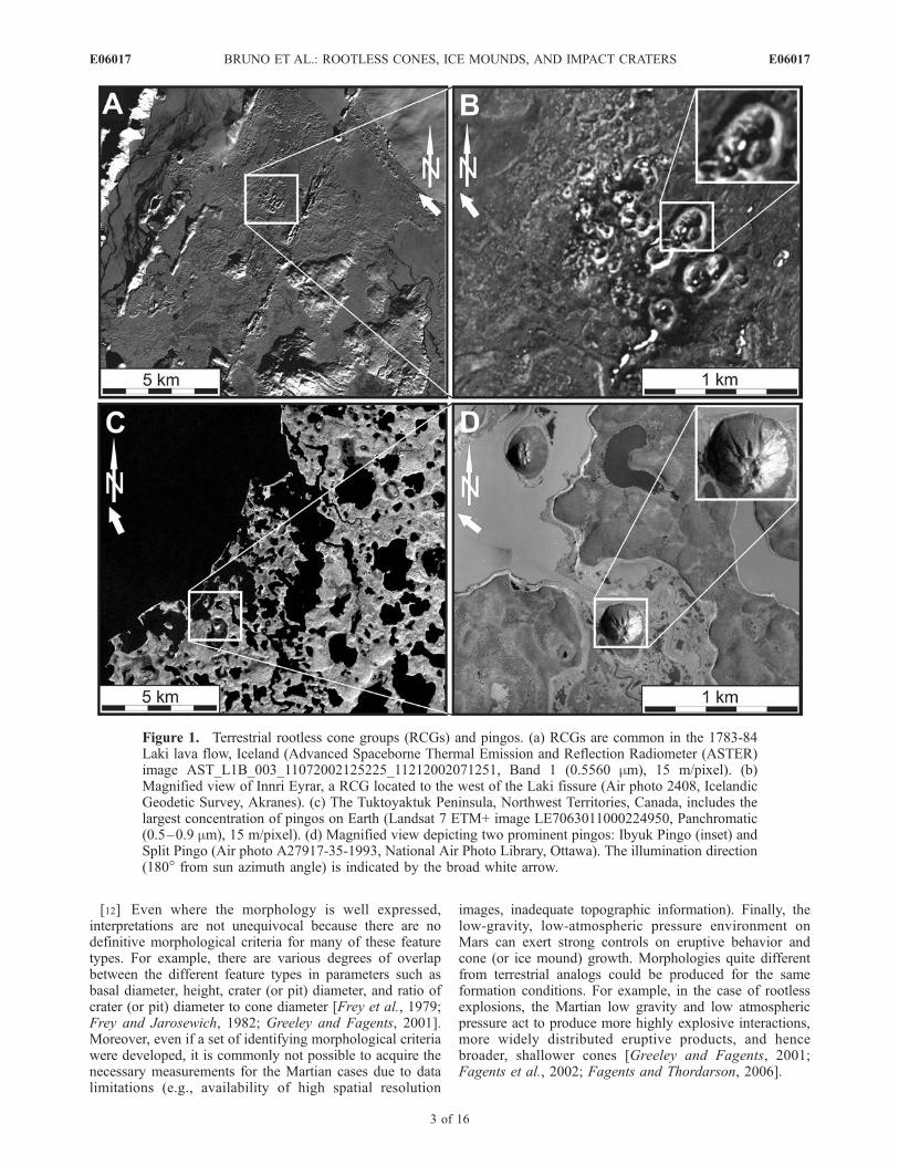
scoria cones, which form over a volcanic conduit moredeeply rooted in the crust to a magma source. Unlikeprimary cones, rootless cones are not the source of lavaflows (although they can feed rheomorphic flows that canbe difficult to distinguish from primary lava flows).Figures 1a and 1b show a typical rootless cone group withinthe 1783-84 Laki lava flow in Iceland. The morphology andspatial density of rootless cones provide an indication of thequantity and location of water in the substrate at the time ofcone formation; modeling the dynamics of cone-formingexplosions permits assessment of the vapor mass andpressure required to produce cones of the observed numbersand sizes [Greeley and Fagents, 2001]. If rootless cones canbe unequivocally identified on Mars, we will have apowerful means to gauge the amount, distribution, andevolution of near-surface volatiles in the regolith.[5] Similarly, the putative identification of pingos and

other ice mounds on Mars implies the presence of volatilesin the Martian regolith [Lucchitta, 1981; Parker et al., 1993;Cabrol et al., 2000; Burr et al., 2005; Soare et al., 2005]. Apingo is a type of ice cored mound, common in periglacialenvironments within Alaska, Canada, and Russia. Likerootless cones, pingos can grow up to several hundreds ofmeters in basal diameter and up to tens of meters in height[Washburn, 1973].[6] In general, pingos form when the overburden is

domed above a segregated ice body that grows either by(1) intrusion and subsequent freezing of liquid waterinjected into permafrost; (2) progressive underplating ofan ice cored mound as an underlying water reservoirfreezes; or (3) a combination of both these processes[Washburn, 1973; Mackay, 1987]. Depending on theirformation mechanism, pingos are divided into two maincategories: hydrostatic and hydraulic.[7] The majority of terrestrial pingos are hydrostatic

(‘‘closed-system’’) pingos and form in response to thedraining of ephemeral ponds and lakes which exposes theunfrozen basin to subfreezing temperatures [Porsild, 1938;Muller, 1959; Mackay, 1962, 1973, 1979, 1998; Washburn,1973]. Progradation of the freezing front both from theground surface downward and the underlying permafrostupward pressurizes the residual pore water. In transmissivesediments, this pore water flows ahead of the freezing fronttoward the basin center, the usual site of minimal permafrostgrowth. Continued flow and freezing of this expelled porewater, in addition to a small effect from volumetric expan-sion, domes up the overlying permafrost layer to form amound [Mackay, 1998; Burr et al., 2005]. Continuedgrowth can produce radial tension fractures from the sum-mit and circumferential compression fractures at the mar-gins. Pingo collapse may occur when the summit rupturesand the remaining liquid water below the ice moundescapes. Collapsed pingos typically form a depressionsurrounded by a raised ring of residual sediment.Figures 1c and 1d show hydrostatic pingos from theTuktoyaktuk Peninsula, Canada.[8] Hydraulic (‘‘open-system’’) pingos tend to form in

narrow valleys or on slopes in areas of discontinuous (orlocally thinner) permafrost. In these cases, artesian pressure

forces water to intrude into shallow permafrost. Uponfreezing, the water ice uplifts the overburden to formmounds [Washburn, 1973]. Hydraulic pingos may alsogrow as a result of hydraulic lift, where low artesianpressure is amplified through confinement under a pingo[Muller, 1959; Holmes et al., 1968]. When discussing icecored mounds of uncertain origin, we use the general term‘‘ice mound’’ (rather than the specific term ‘‘pingo’’) toinclude other segregated ice bodies such as palsas, hydro-laccoliths, icings, and ice hummocks. (SeeWashburn [1973]for a comprehensive description of these features.) Wereserve the term ‘‘pingo’’ for ice cored mounds of knownhydraulic or hydrostatic origin.[9] On Mars, potential rootless volcanic cones have been

identified in the northern lowland plains (Figure 2a),including Acidalia, Amazonis, Isidis, and Elysium Planitiae[Allen, 1979a; Frey and Jarosewich, 1982; Greeley andFagents, 2001; Lanagan et al., 2001; Fagents et al., 2002].Possible Martian ice mounds have been identified in GusevCrater, Athabasca Valles and the Cerberus Plains (Figure 2b)as defined by Plescia [1990], and Chryse, Acidalia, andUtopia Planitiae [Lucchitta, 1981; Parker et al., 1993;Cabrol et al., 2000; Burr et al., 2005; Soare et al., 2005;Page and Murray, 2006].[10] Historically, Martian pingos have been difficult to

identify on the basis of Viking Orbiter data, in part becauseof limited availability of high-resolution images, but alsobecause only the most mature pingos exhibit distinctivemorphologies. Younger and/or smaller pingos are typicallyexpressed as low-relief mounds. Only once the mound issufficiently upheaved does its surface begin to rupture,thereby exposing the interior ice, which melts or sublimesto form crevices and pits at or near the summit [Washburn,1973;Mackay, 1979]. Moreover, these morphologies are aptto be confused with those of rootless cones, and thepresence of pingos or other ice mounds on Mars remainsequivocal [Theilig and Greeley, 1979; Lucchitta, 1981;Rossbacher and Judson, 1981; Squyres et al., 1992; Parkeret al., 1993; Cabrol et al., 2000].[11] Geological context is therefore of key importance in

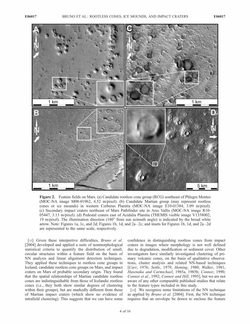
identifying rootless cones and ice mounds. Interpretation ofa volcanic origin is relatively straightforward for pristinecones lying on surfaces with clear textural indications oflava flow morphology [Lanagan et al., 2001]. However, inareas where the cones and/or the underlying surface aredegraded or mantled by dust, or for which image resolutionis a limiting factor, it becomes harder to identify the originson the basis of morphology alone. Ambiguities arise be-cause, under these adverse conditions, other small, circular,pitted cones or mounds can resemble rootless cones. Inaddition to the ice mound hypothesis, other possibilitiesinclude (1) secondary (Figure 2c) or pedestal (Figure 2d)impact craters, the latter having resistant ejecta armoring amore easily eroded substrate; (2) mud volcanoes producedby gas- or water-charged eruptions of clastic sediments[Tanaka, 1997; Farrand et al., 2005]; (3) primary scoriacones; (4) gravity craters, produced when blocks of icetransported by jokulhlaups (glacial outburst floods) settleinto soft sediments [Gaidos and Marion, 2003]; and (5)kettle holes, which are formed when sediment-laden iceblocks are partially buried and subsequently melted [Gaidosand Marion, 2003].

E06017 BRUNO ET AL.: ROOTLESS CONES, ICE MOUNDS, AND IMPACT CRATERS

2 of 16

E06017

[12] Even where the morphology is well expressed,interpretations are not unequivocal because there are nodefinitive morphological criteria for many of these featuretypes. For example, there are various degrees of overlapbetween the different feature types in parameters such asbasal diameter, height, crater (or pit) diameter, and ratio ofcrater (or pit) diameter to cone diameter [Frey et al., 1979;Frey and Jarosewich, 1982; Greeley and Fagents, 2001].Moreover, even if a set of identifying morphological criteriawere developed, it is commonly not possible to acquire thenecessary measurements for the Martian cases due to datalimitations (e.g., availability of high spatial resolution

images, inadequate topographic information). Finally, thelow-gravity, low-atmospheric pressure environment onMars can exert strong controls on eruptive behavior andcone (or ice mound) growth. Morphologies quite differentfrom terrestrial analogs could be produced for the sameformation conditions. For example, in the case of rootlessexplosions, the Martian low gravity and low atmosphericpressure act to produce more highly explosive interactions,more widely distributed eruptive products, and hencebroader, shallower cones [Greeley and Fagents, 2001;Fagents et al., 2002; Fagents and Thordarson, 2006].

Figure 1. Terrestrial rootless cone groups (RCGs) and pingos. (a) RCGs are common in the 1783-84Laki lava flow, Iceland (Advanced Spaceborne Thermal Emission and Reflection Radiometer (ASTER)image AST_L1B_003_11072002125225_11212002071251, Band 1 (0.5560 mm), 15 m/pixel). (b)Magnified view of Innri Eyrar, a RCG located to the west of the Laki fissure (Air photo 2408, IcelandicGeodetic Survey, Akranes). (c) The Tuktoyaktuk Peninsula, Northwest Territories, Canada, includes thelargest concentration of pingos on Earth (Landsat 7 ETM+ image LE7063011000224950, Panchromatic(0.5–0.9 mm), 15 m/pixel). (d) Magnified view depicting two prominent pingos: Ibyuk Pingo (inset) andSplit Pingo (Air photo A27917-35-1993, National Air Photo Library, Ottawa). The illumination direction(180� from sun azimuth angle) is indicated by the broad white arrow.


3 of 16

E06017

[13] Given these interpretive difficulties, Bruno et al.[2004] developed and applied a suite of nonmorphologicalstatistical criteria to quantify the distribution of small,circular structures within a feature field on the basis ofNN analysis and linear alignment detection techniques.They applied these techniques to rootless cone groups inIceland, candidate rootless cone groups on Mars, and impactcraters on Mars of probable secondary origin. They foundthat the spatial relationships of Martian candidate rootlesscones are indistinguishable from those of Icelandic rootlesscones (i.e., they both show similar degrees of clusteringwithin their groups), but are markedly different from thoseof Martian impact craters (which show no evidence ofintrafield clustering). This suggests that we can have some

confidence in distinguishing rootless cones from impactcraters in images where morphology is not well defineddue to degradation, modification or sediment cover. Otherinvestigators have similarly investigated clustering of pri-mary volcanic cones, on the basis of qualitative observa-tions, cluster analysis and related NN-based techniques[Carr, 1976; Settle, 1979; Heming, 1980; Walker, 1981;Hasenaka and Carmichael, 1985a, 1985b; Connor, 1990;Connor et al., 1992; Connor and Hill, 1995], but we are notaware of any other comparable published studies that relateto the feature types included in this study.[14] We recognize some limitations of the NN technique

as applied by Bruno et al. [2004]. First, the NN techniquerequires that an envelope be drawn to enclose the feature

Figure 2. Feature fields on Mars. (a) Candidate rootless cone group (RCG) southeast of Phlegra Montes(MOC-NA image M08-01962, 4.52 m/pixel). (b) Candidate Martian group (may represent rootlesscones or ice mounds) in western Cerberus Planitia (MOC-NA image E10-01384, 3.09 m/pixel).(c) Secondary impact craters northeast of Mars Pathfinder site in Ares Vallis (MOC-NA image R10-05447, 3.13 m/pixel). (d) Pedestal craters east of Acidalia Planitia (THEMIS visible image V1358002,19 m/pixel). The illumination direction (180� from sun azimuth angle) is indicated by the broad whitearrow. Note: Figures 1a, 1c, and 2d; Figures 1b, 1d, and 2a–2c; and insets for Figures 1b, 1d, and 2a–2dare represented to the same scale, respectively.


4 of 16

E06017

field. Bruno et al. [2004] used the best fitting rectangle toenclose all cones or craters in a given group, but there are anumber of reasons why this is not the best approach (asdiscussed below). Second, features which occur along theborder of an image were fully included as members of thegroup. However, our inability to assess their nearest neigh-bors (which might be beyond the edge of the image)suggests that they should be selectively excluded from theanalysis. The third issue is group definition. Several featurefields contain subclusters within them, and treating allfeatures as a single group can considerably affect NNresults. Finally, and perhaps most important, standard NNmethodology reduces all the information of a feature field totwo statistics (R and c), and much important information islost in this process.[15] In this paper we present refinements to standard NN

methodology in the areas outlined above, and this leads to amore objective assessment of spatial distribution. We applyour methodology to the same data set studied by Bruno etal. [2004], as well as to terrestrial ice mounds, candidateMartian ice mounds, and Martian pedestal craters for thefirst time. Finally, we outline a skewness-kurtosis analysiswhich, when combined with the standard NN statistics Rand c, proves useful in separating feature types.[16] Throughout this paper, we use the term ‘‘random.’’

Spatial randomness is defined for a set of points on a givenarea as follows: ‘‘any point has had the same chance ofoccurring on any subarea as any other point; that anysubarea of specified size has had the same chance ofreceiving a point as any other subarea of that size, and thatthe placement of each point has not been influenced by thatof any other point’’ [Clark and Evans, 1954]. Thus spatialrandomness is intimately connected with a Poisson proba-bility distribution of points in a plane of infinite extent. Inthis work, we are concerned only with spatial randomnessresulting from an underlying Poisson distribution and itscorresponding probability distribution of nearest neighbordistances. Therefore we use the term ‘‘random’’ as aconvenient shorthand for these concepts.

2. Data

2.1. Icelandic Rootless Cones (8 Groups)

[17] For our first data set, we apply our refined NNmethodology to the same three Icelandic lava flow fields

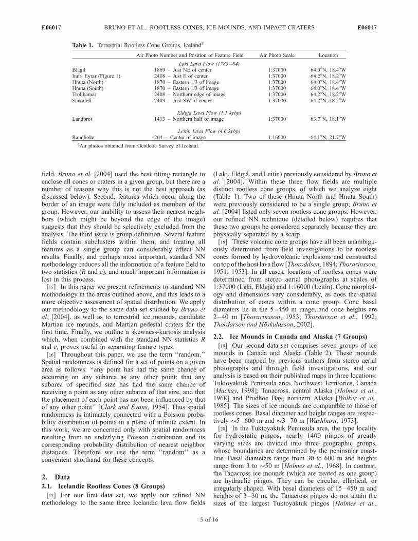
(Laki, Eldgja, and Leitin) previously considered by Bruno etal. [2004]. Within these three flow fields are multipledistinct rootless cone groups, of which we analyze eight(Table 1). Two of these (Hnuta North and Hnuta South)were previously considered to be a single group; Bruno etal. [2004] listed only seven rootless cone groups. However,our refined NN technique (detailed below) requires thatthese two groups be considered separately because they arephysically separated by a scarp.[18] These volcanic cone groups have all been unambigu-

ously determined from field investigations to be rootlesscones formed by hydrovolcanic explosions and constructedon top of the host lava flow [Thoroddsen, 1894;Thorarinsson,1951; 1953]. In all cases, locations of rootless cones weredetermined from stereo aerial photographs at scales of1:37000 (Laki, Eldgja) and 1:16000 (Leitin). Cone morphol-ogy and dimensions vary considerably, as does the spatialdistribution of cones within a cone group. Cone basaldiameters lie in the 5–450 m range, and cone heights are2–40 m [Thorarinsson, 1953; Thordarson et al., 1992;Thordarson and Hoskuldsson, 2002].

2.2. Ice Mounds in Canada and Alaska (7 Groups)

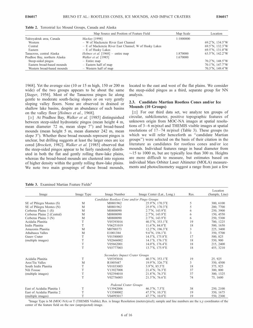
[19] Our second data set comprises seven groups of icemounds in Canada and Alaska (Table 2). These moundshave been mapped by previous authors from stereo aerialphotographs and through field investigations, and ouranalysis is based on their published maps in three locations:Tuktoyaktuk Peninsula area, Northwest Territories, Canada[Mackay, 1998]; Tanacross, central Alaska [Holmes et al.,1968] and Prudhoe Bay, northern Alaska [Walker et al.,1985]. The sizes of ice mounds are comparable to those ofrootless cones. Basal diameter and height ranges are respec-tively �5–600 m and �3–70 m [Washburn, 1973].[20] In the Tuktoyaktuk Peninsula area, the type locality

for hydrostatic pingos, nearly 1400 pingos of greatlyvarying sizes are divided into three geographic groups,whose boundaries are determined by the peninsular coast-line. Basal diameters range from 30 to 600 m and heightsrange from 3 to �50 m [Holmes et al., 1968]. In contrast,the Tanacross ice mounds (which are treated as one group)are hydraulic pingos. They can be circular, elliptical, orirregularly shaped. With basal diameters of 15–450 m andheights of 3–30 m, the Tanacross pingos do not attain thesizes of the largest Tuktoyaktuk pingos [Holmes et al.,

Table 1. Terrestrial Rootless Cone Groups, Icelanda

Air Photo Number and Position of Feature Field Air Photo Scale Location

Laki Lava Flow (1783–84)Blagil 1869 – Just NE of center 1:37000 64.0�N, 18.4�WInnri Eyrar (Figure 1) 2408 – Just E of center 1:37000 64.2�N, 18.2�WHnuta (North) 1870 – Eastern 1/3 of image 1:37000 64.0�N, 18.4�WHnuta (South) 1870 – Eastern 1/3 of image 1:37000 64.0�N, 18.4�WTrollhamar 2408 – Northern edge of image 1:37000 64.2�N, 18.2�WStakafell 2409 – Just SW of center 1:37000 64.2�N, 18.2�W

Eldgja Lava Flow (1.1 kybp)Landbrot 1413 – Northern half of image 1:37000 63.7�N, 18.1�W

Leitin Lava Flow (4.6 kybp)Raudholar 264 – Center of image 1:16000 64.1�N, 21.7�W

aAir photos obtained from Geodetic Survey of Iceland.


5 of 16

E06017

1968]. Yet the average size (10 or 15 m high, 150 or 200 mwide) of the two groups appears to be about the same[Stager, 1956]. Most of the Tanacross pingos lie alonggentle to moderate south-facing slopes or on very gentlysloping valley floors. None are observed in drained orshallow lake basins, despite an abundance of such basinson the valley floor [Holmes et al., 1968].[21] At Prudhoe Bay, Walker et al. [1985] distinguished

between steep-sided hydrostatic pingos (mean height 4 m,mean diameter 72 m, mean slope 7�) and broad-basedmounds (mean height 5 m, mean diameter 242 m, meanslope 3�). Whether these broad mounds represent pingos isunclear, but drilling suggests at least the larger ones are icecored [Brockett, 1982]. Walker et al. [1985] observed thatthe steep-sided pingos appear to be fairly randomly distrib-uted in both the flat and gently rolling thaw-lake plains,whereas the broad-based mounds are clustered into regionsof higher density within the gently rolling thaw-lake plains.We note two main groupings of these broad mounds,

located to the east and west of the flat plains. We considerthe steep-sided pingos as a third, separate group for NNanalysis.

2.3. Candidate Martian Rootless Cones and/or IceMounds (10 Groups)

[22] For our third data set, we analyze ten groups ofcircular, subkilometer, positive topographic features ofunknown origin from MOC-NA images at spatial resolu-tions of 3–6 m/pixel and THEMIS visible images at spatialresolutions of 17–74 m/pixel (Table 3). These groups (towhich we will refer henceforth as ‘‘candidate Martiangroups’’) were selected on the basis of their citation in theliterature as candidates for rootless cones and/or icemounds. Individual features range in basal diameter from�15 to 1000 m, but are typically less than 300 m. Heightsare more difficult to measure, but estimates based onindividual Mars Orbiter Laser Altimeter (MOLA) measure-ments and photoclinometry suggest a range from just a few

Table 2. Terrestrial Ice Mound Groups, Canada and Alaska

Map Source and Position of Feature Field Map Scale Location

Tuktoyaktuk area, Canada Mackay [1998] 1:1000000Western – W of Mackenzie River East Channel 69.2�N, 134.5�WCentral – E of Mackenzie River East Channel; W of Husky Lakes 69.5�N, 132.3�WEastern – E of Husky Lakes 69.5�N, 131.0�W

Tanacross, central Alaska Holmes et al. [1968] – entire map 1:870000 63.5�N, 142.2�WPrudhoe Bay, northern Alaska Walker et al. [1985] 1:670000

Steep-sided pingos – Entire map 70.2�N, 148.5�WEastern broad-based mounds – Eastern half of map 70.1�N, 147.7�WWestern broad-based mounds – Western half of map 70.3�N, 149.4�W

Table 3. Examined Martian Feature Fieldsa

Image Image Type Image Number Image Center (Lat., Long.) Res.Location

(Sample, Line)

Candidate Rootless Cone and/or Pingo GroupsSE of Phlegra Montes (S) M M0801962 25.9�N, 170.3�E 5 300, 6100SE of Phlegra Montes (N) M M0801962 25.9�N, 170.3�E 5 200, 7700Cerberus Plains 1 (S) M M0800090 2.7�N, 143.9�E 6 250, 3900Cerberus Plains 2 (Central) M M0800090 2.7�N, 143.9�E 6 150, 4550Cerberus Plains 3 (N) M M0800090 2.7�N, 143.9�E 6 250, 5300Acidalia Planitia T V05393016 40.3�N, 353.1�E 19 700, 1225Isidis Planitia T V06251019 11.6�N, 84.8�E 18 500, 1650Amazonis Planitia M M0700373 12.2�N, 196.3�E 3 225, 3400Athabasca Valles M E1001384 9.6�N, 156.1�E 3 350, 5700Gusev Crater T V01580003 14.5�S, 175.8�E 17 500, 825(multiple images) T V02666002 14.1�S, 176.1�E 18 550, 900

T V05662001 14.0�S, 176.4�E 18 215, 2400T V03777003 13.7�S, 175.9�E 18 455, 3210

Secondary Impact Crater GroupsAcidalia Planitia T V05393016 40.3�N, 353.1�E 19 25, 925Ares/Tiu Valles M R1005447 19.9�N, 326.7�E 3 350, 4500South Isidis Planitia T V01033003 3.9�N, 85.5�E 18 375, 925Nili Fossae T V13927008 21.4�N, 76.3�E 37 300, 800(multiple images) T V02394010 21.8�N, 76.3�E 37 300, 1325

T V02756003 21.3�N, 76.6�E 74 75, 1600

Pedestal Crater GroupsEast of Acidalia Planitia 1 T V13942006 46.3�N, 7.5�E 38 250, 2100East of Acidalia Planitia 2 T V13580002 47.5�N, 10.3�E 19 350, 1675(multiple images) T V04993017 47.7�N, 10.0�E 19 550, 2300

aImage Type is M (MOC-NA) or T (THEMIS Visible); Res. is Image Resolution (meters/pixel); sample and line numbers are the x,y coordinates of thecenter of the feature field on the raw (unprojected) image.


6 of 16

E06017

meters at Athabasca Valles to close to 100 m at GusevCrater [Cabrol et al., 2000; Burr et al., 2005; Soare et al.,2005].[23] Two of these candidate Martian groups are located

southeast of Phlegra Montes and west of Amazonis Planitia(MOC-NA image M0801962). Here, features have beeninterpreted as rootless cones on the basis of a variety ofcriteria, including distinct conical morphology and welldefined summit craters, stratigraphic position atop a lavaflow having a pristine platy-ridged surface texture, the lackof association with eruptive fissures, and an absence of lavaflows issuing from the cones [Greeley and Fagents, 2001;Lanagan et al., 2001]. Three candidate Martian groups arelocated in the region Plescia [1990, 1993, 2003] called theCerberus plains (MOC-NA image M0800090). These fea-tures have similarly been interpreted as rootless cones onthe basis of distinctive morphologies and geologic relations[Lanagan et al., 2001].[24] The morphologies of cone-like features in the Cydo-

nia region of Acidalia Planitia (THEMIS imageV05393016) and within Isidis Planitia (THEMIS imageV06251019) are less pristine. These two groups containdegraded, positive-relief, conical features with subduedsummit craters (e.g., Figure 2a) that are quite distinct fromthe impact craters located within the same images. Conesand mounds in these areas were interpreted as rootless coneson the basis of Viking Orbiter imagery [Frey et al., 1979;Frey and Jarosewich, 1982]. The surfaces on which thefeatures reside appear considerably older than those inMOC-NA images M0800090 and M0801962, as evidencedby the higher density of impact craters. One possibility isthat the cones formed on a sedimentary surface, in whichcase they could not be volcanic, let alone rootless. Alterna-tively, the original surface prior to mantling may have beenlava that, in combination with a volatile-rich substrate,would admit the possibility of rootless cone formation.The Isidis cones have also been interpreted as pingos; theircratered expression has been attributed to ablation of icecores within ice mounds [Rossbacher and Judson, 1981;Grizzaffi and Schultz, 1989]. However, the influx into thebasin of voluminous flows from Syrtis Major (immediatelyto the west) suggests that significant lava resurfacing oncetook place and may have provided conditions favorable forrootless cone formation.[25] In Amazonis Planitia, the confluence of recent vol-

canism and recent fluvial activity allows for the possibilityof both pingo growth and rootless cone formation [Burr etal., 2002a, 2002b]. MOC-NA image M0700373 shows agroup of mounds and cones lying on an older, degradedsurface. Lanagan et al. [2001] interpreted these mounds tobe rootless cones.[26] Recently acquired high-resolution MOC-NA images

have revealed possible pingo forms in great detail. Oneparticular group of features in Athabasca Valles (Figure 2b)has been imaged at resolutions as high as 1.5–3 m/pixel.Basal diameters lie in the range 15–128 m; heights are inthe range 1.5–24 m [Burr et al., 2005]. The continuum ofmorphologies exhibited in this image, ranging from circularmounds and pitted cones to irregularly shaped depressionswith positive relief margins, is less characteristic of rootlessvolcanic cones. Furthermore, the association of these fea-tures with a sedimentary substrate in an outflow channel has

been cited as corroborating evidence that these features arepingos, collapsing pingos, and residual pingo scars [Burr etal., 2005]. An alternate interpretation for the low, rimmeddepressions is that they are kettle holes or gravity craters[Gaidos and Marion, 2003].[27] The final candidate Martian group is located along

the margins of Thira Crater, located to the east of the MarsExploration Rover, Spirit, landing site within Gusev Crater(Figure 3). On the basis of geomorphological interpretationof Viking Orbiter imagery, Cabrol et al. [2000] proposedthese enigmatic mounds are pingos that formed shortly afterthe impact that created Thira Crater. Using higher resolutionTHEMIS visible imagery (V01580003; V02666002;V05662001; V03777003), we are able to identify 93 suchmounds, almost three times the number originally identifiedby Cabrol et al. [2000].

2.4. Martian Impact Craters (6 Groups)

2.4.1. Martian Secondary Impact Craters (4 Groups)[28] Of the six groups of Martian impact craters in our

analysis, four represent probable secondary impact crateringevents: Ares/Tiu Valles (imaged by MOC-NA at a resolu-tion of 13 m/pixel), Acidalia Planitia, Nili Fossae, and southIsidis Planitia (all imaged by THEMIS at resolutions of 17–74 m/pixel) (Table 3). The largest craters are found at NiliFossae, with diameters ranging up to 1.5 km. In the otherthree groups, craters are subkilometer in diameter. Thesefeatures have been identified as probable secondary impactcraters on the basis of their impact morphologies, occur-rence in tight groupings and a qualitative inspection of theirsize-frequency distributions.2.4.2. Martian Pedestal Craters (2 Groups)[29] The final two groups of Martian impact craters

included in this analysis have been previously identifiedas pedestal craters by other investigators [e.g., Carr, 1981].Both groups are located just east of Acidalia Planitia, andwere analyzed from THEMIS images at resolutions of 19–38 m/pixel (Table 3). Pedestal craters are believed to take ona highstanding expression when the surrounding surfaceundergoes substantial eolian erosion: the crater ejectaarmors the underlying material, thereby protecting it fromerosion. In some cases, pedestal crater ejecta take onbroad, pancake-like morphologies. However, smaller exam-ples with less extensive ejecta blankets are more conical,and hence more apt to be confused with volcanic conestructures.[30] The six secondary and pedestal crater groups are

included in this study to determine whether the spatialdistributions of either or both impact crater types can beremotely distinguished from rootless cones and/or icemounds. If the spatial distributions of these impact cratertypes are found to be statistically different from those ofrootless cones and/or ice mounds, then NN analysis can beused to distinguish rootless cones and/or ice mounds fromimpact craters in images where morphology is not welldefined due to degradation, modification or sediment cover.This assumes, however, that any such modification wouldnot completely obliterate any feature or cause crater satu-ration, which would likely affect the spatial statistics. (SeeSquyres et al. [1997] for a discussion of the effect of cratersaturation and obliteration on spatial statistics.)


7 of 16

E06017

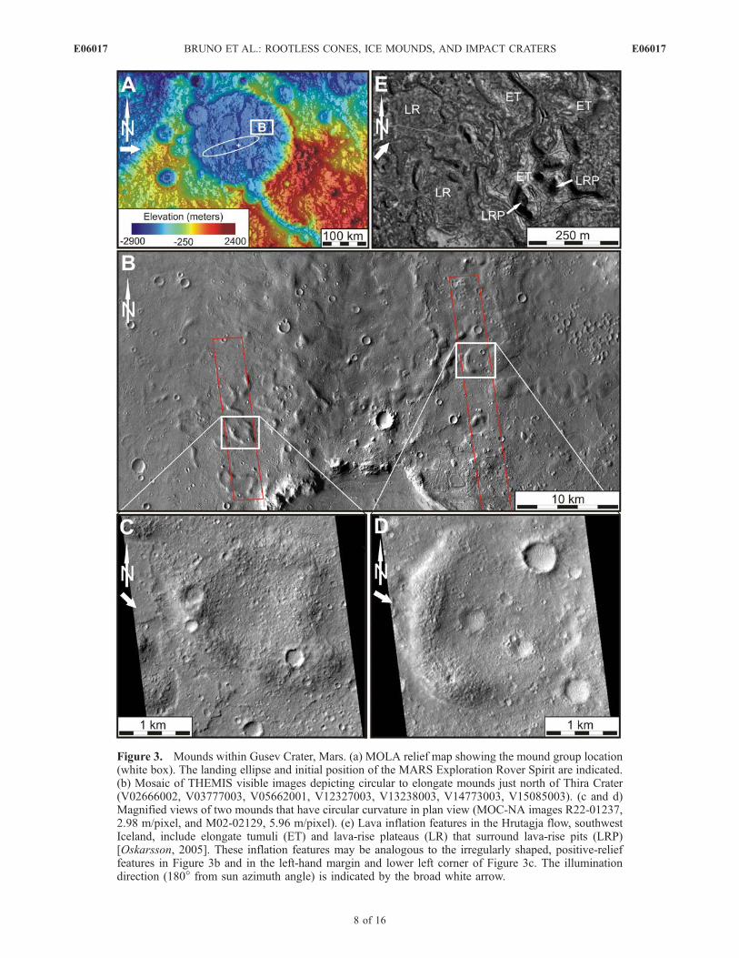
Figure 3. Mounds within Gusev Crater, Mars. (a) MOLA relief map showing the mound group location(white box). The landing ellipse and initial position of the MARS Exploration Rover Spirit are indicated.(b) Mosaic of THEMIS visible images depicting circular to elongate mounds just north of Thira Crater(V02666002, V03777003, V05662001, V12327003, V13238003, V14773003, V15085003). (c and d)Magnified views of two mounds that have circular curvature in plan view (MOC-NA images R22-01237,2.98 m/pixel, and M02-02129, 5.96 m/pixel). (e) Lava inflation features in the Hrutagja flow, southwestIceland, include elongate tumuli (ET) and lava-rise plateaus (LR) that surround lava-rise pits (LRP)[Oskarsson, 2005]. These inflation features may be analogous to the irregularly shaped, positive-relieffeatures in Figure 3b and in the left-hand margin and lower left corner of Figure 3c. The illuminationdirection (180� from sun azimuth angle) is indicated by the broad white arrow.


8 of 16

E06017

[31] We note that other layered ejecta craters (e.g., single-layer, double-layer, or multiple-layer ejecta craters) [Barlowet al., 2000], which are thought to form by emplacement offluidized ejecta flows due to the presence of volatiles in thesubstrate [Carr et al., 1977; Gault and Greeley, 1978;Mouginis-Mark, 1987] or through atmospheric effects[Schultz and Gault, 1979; Schultz, 1992; Barnouin-Jhaand Schultz, 1996, 1998], typically exceed 4 km in diameterand exhibit quite distinctive morphologies. These craters aretherefore unlikely to be mistaken for the subkilometer scaleof rootless cones, pingos, and other ice mounds, and are notincluded in our analysis.

3. Methodology

3.1. Review of Standard Nearest NeighborMethodology

[32] The NN technique quantifies the degree of spatialrandomness of features within a plane and provides a meansfor evaluating the statistical significance of deviations frompurely random. For detailed information on this method,including the underlying equations and derivations, refer toClark and Evans [1954]. This technique can readily beapplied to any feature type (e.g., primary or rootlessvolcanic cones, ice mounds, impact craters, lakes, kettleholes): it simply requires a map or image in which eachfeature is represented by a point. This methodologyinvolves first measuring r, the distance between each pointand its NN. In cases where cones contain multiple craters,each crater is considered to be a separate feature. We thenaverage these distances together to arrive at Ra, the averageactual distance between each pair of NNs:

Ra ¼Srn

ð1Þ

where n is the number of features in the group. (Allequations are from Clark and Evans [1954].) Next, wecalculate Re, the average NN spacing that would beexpected if the same number of features were distributedat random throughout the given field area:

Re ¼1

2ffiffiffir

p ð2Þ

where r is the density of the feature field (i.e., number offeatures divided by field area). The ratio of Ra and Re yieldsthe dimensionless statistic R, which quantifies any departurefrom the expected random spacing of nearest neighbors, i.e.,

R ¼ Ra

Re

ð3Þ

By definition, randomly distributed cones would beexpected to have Ra � Re, yielding R � 1. Large valuesof R (R > 1) indicate that features are spaced further apartthan would be expected from a Poisson NN distribution(i.e., Ra > Re), as exemplified, in the limit, by a distributionof evenly spaced features. Small values of R (R < 1) reflectintragroup clustering: within a given group, features tend tooccur more closely than would be expected at random (i.e.,Ra < Re).

[33] The key test statistic for evaluating whether anobserved distribution is consistent with a random Poissondistribution is c:

c ¼ Ra � Re

sRe

ð4Þ

where sReis the standard error of the mean of the NN

distances in a randomly distributed population. At the 0.05significance level, the critical value of c is 1.96: jcj > 1.96indicates statistically significant nonrandomness.

3.2. Field Area Selection

3.2.1. Convex Hull Methodology and Treatmentof Border Features[34] In their study of rootless cone groups, Bruno et al.

[2004] defined the field area as the smallest externalrectangle containing all cones in the field. However, byrequiring the area to be rectangular, some degree of ‘‘emptyspace’’ was inherently added to each cone field. Moreover,field shape had an unintended influence on the final result,with rectangular fields having less dead space (and thereforetending to appear less clustered) than other field shapes.[35] In this paper, we use the ‘‘convex hull’’ to define the

natural boundary of a feature field [Graham, 1972]. Thisprovides an improvement over prior analysis by diminishingareas in images that can distort statistical testing of spatialrandomness. Here, the field area is defined as a convexpolygon (i.e., a polygon with each interior angle measuringless than 180�), whose vertices are determined by theoutermost features in the field. The convex hull is thereforethe smallest convex polygon containing all features within afield and its perimeter will be the shortest path enclosing allpoints [Graham, 1972].[36] Features which occur along the external edges of the

group (i.e., lie on the convex hull) are selectively excludedfrom the analysis due to our inability to confidently locatetheir NN, which might lie beyond the edge of the image.These border features may serve as a NN to an interiorfeature, but they are excluded from the set of points thatselect a NN. For consistency, we apply this treatment to allborder features for all feature fields, even in those caseswhere we are confident that all features are contained in theimage. Figure 4 illustrates the convex hull methodology andtreatment of border features on sample synthetic and naturaldata.3.2.2. Spatial Subsets and Cluster Definition[37] Depending on the distribution, the NN methodology

can be highly sensitive to choice of spatial subset (Figure 4,Table 4). For self-similar (e.g., Poisson and evenly spaced)distributions, choosing a subset of the feature field shouldhave little effect on NN results provided there are asufficiently large number of features. Exactly how manyfeatures are required for a robust analysis is unclear. Table 4suggests that 30 or 40 features may be sufficient, providedthat the spatial distribution of the subset is representative ofthe feature field as a whole. However, if only a spatialsubset of the feature field is available for analysis (e.g., dueto limited imaging or mapping), it is impossible to discernwhether the available data constitutes a representativesubset so NN results cannot be generalized to the entirefeature field.


9 of 16

E06017

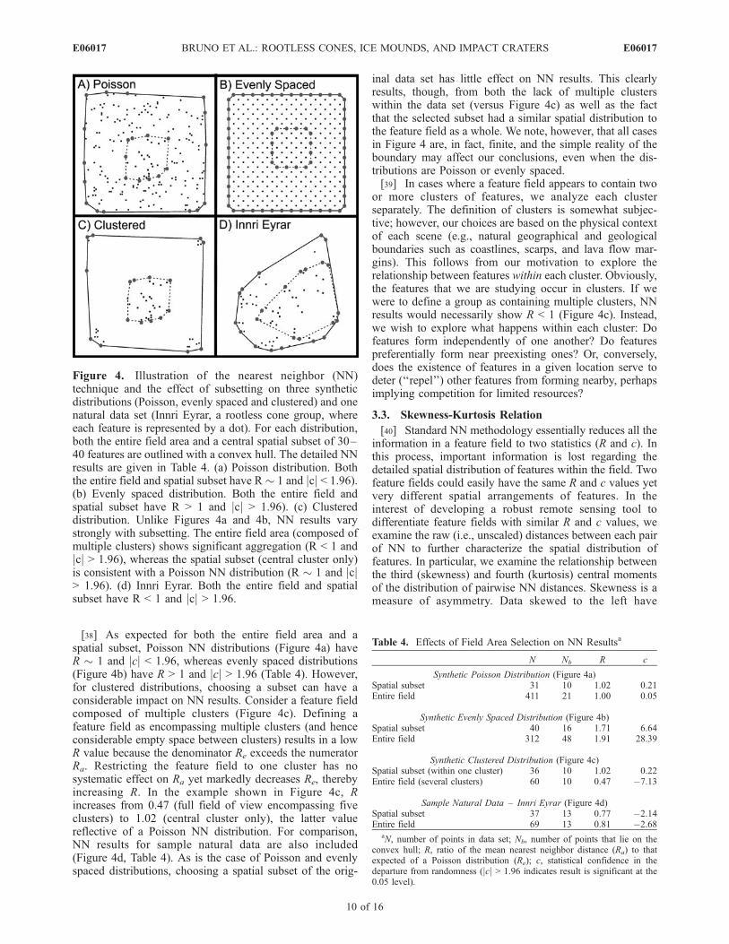
[38] As expected for both the entire field area and aspatial subset, Poisson NN distributions (Figure 4a) haveR � 1 and jcj < 1.96, whereas evenly spaced distributions(Figure 4b) have R > 1 and jcj > 1.96 (Table 4). However,for clustered distributions, choosing a subset can have aconsiderable impact on NN results. Consider a feature fieldcomposed of multiple clusters (Figure 4c). Defining afeature field as encompassing multiple clusters (and henceconsiderable empty space between clusters) results in a lowR value because the denominator Re exceeds the numeratorRa. Restricting the feature field to one cluster has nosystematic effect on Ra yet markedly decreases Re, therebyincreasing R. In the example shown in Figure 4c, Rincreases from 0.47 (full field of view encompassing fiveclusters) to 1.02 (central cluster only), the latter valuereflective of a Poisson NN distribution. For comparison,NN results for sample natural data are also included(Figure 4d, Table 4). As is the case of Poisson and evenlyspaced distributions, choosing a spatial subset of the orig-

inal data set has little effect on NN results. This clearlyresults, though, from both the lack of multiple clusterswithin the data set (versus Figure 4c) as well as the factthat the selected subset had a similar spatial distribution tothe feature field as a whole. We note, however, that all casesin Figure 4 are, in fact, finite, and the simple reality of theboundary may affect our conclusions, even when the dis-tributions are Poisson or evenly spaced.[39] In cases where a feature field appears to contain two

or more clusters of features, we analyze each clusterseparately. The definition of clusters is somewhat subjec-tive; however, our choices are based on the physical contextof each scene (e.g., natural geographical and geologicalboundaries such as coastlines, scarps, and lava flow mar-gins). This follows from our motivation to explore therelationship between features within each cluster. Obviously,the features that we are studying occur in clusters. If wewere to define a group as containing multiple clusters, NNresults would necessarily show R < 1 (Figure 4c). Instead,we wish to explore what happens within each cluster: Dofeatures form independently of one another? Do featurespreferentially form near preexisting ones? Or, conversely,does the existence of features in a given location serve todeter (‘‘repel’’) other features from forming nearby, perhapsimplying competition for limited resources?

3.3. Skewness-Kurtosis Relation

[40] Standard NN methodology essentially reduces all theinformation in a feature field to two statistics (R and c). Inthis process, important information is lost regarding thedetailed spatial distribution of features within the field. Twofeature fields could easily have the same R and c values yetvery different spatial arrangements of features. In theinterest of developing a robust remote sensing tool todifferentiate feature fields with similar R and c values, weexamine the raw (i.e., unscaled) distances between each pairof NN to further characterize the spatial distribution offeatures. In particular, we examine the relationship betweenthe third (skewness) and fourth (kurtosis) central momentsof the distribution of pairwise NN distances. Skewness is ameasure of asymmetry. Data skewed to the left have

Table 4. Effects of Field Area Selection on NN Resultsa

N Nb R c

Synthetic Poisson Distribution (Figure 4a)Spatial subset 31 10 1.02 0.21Entire field 411 21 1.00 0.05

Synthetic Evenly Spaced Distribution (Figure 4b)Spatial subset 40 16 1.71 6.64Entire field 312 48 1.91 28.39

Synthetic Clustered Distribution (Figure 4c)Spatial subset (within one cluster) 36 10 1.02 0.22Entire field (several clusters) 60 10 0.47 �7.13

Sample Natural Data – Innri Eyrar (Figure 4d)Spatial subset 37 13 0.77 �2.14Entire field 69 13 0.81 �2.68

aN, number of points in data set; Nb, number of points that lie on theconvex hull; R, ratio of the mean nearest neighbor distance (Ra) to thatexpected of a Poisson distribution (Re); c, statistical confidence in thedeparture from randomness (jcj > 1.96 indicates result is significant at the0.05 level).

Figure 4. Illustration of the nearest neighbor (NN)technique and the effect of subsetting on three syntheticdistributions (Poisson, evenly spaced and clustered) and onenatural data set (Innri Eyrar, a rootless cone group, whereeach feature is represented by a dot). For each distribution,both the entire field area and a central spatial subset of 30–40 features are outlined with a convex hull. The detailed NNresults are given in Table 4. (a) Poisson distribution. Boththe entire field and spatial subset have R � 1 and jcj < 1.96).(b) Evenly spaced distribution. Both the entire field andspatial subset have R > 1 and jcj > 1.96). (c) Clustereddistribution. Unlike Figures 4a and 4b, NN results varystrongly with subsetting. The entire field area (composed ofmultiple clusters) shows significant aggregation (R < 1 andjcj > 1.96), whereas the spatial subset (central cluster only)is consistent with a Poisson NN distribution (R � 1 and jcj> 1.96). (d) Innri Eyrar. Both the entire field and spatialsubset have R < 1 and jcj > 1.96.


10 of 16

E06017

negative skewness, whereas data skewed to the right havepositive values. Kurtosis is the degree of peakedness of adistribution; higher values indicate distributions with simul-taneously sharper peaks and fatter tails. As these momentsdistinguish standard distributions from each other, thisaspect of the methodology is designed to rapidly differen-tiate the NN distributions from each other without adetailed analysis of the full histogram of NN distances.There are a variety of formulae to estimate the skewnessand kurtosis of distributions. We use the following fairlystandard formulations:

Skewnessn

n� 1ð Þ n� 2ð ÞXni¼1

ri � Ra

s

� �3

ð5Þ

Kurtosis

n nþ 1ð Þn� 1ð Þ n� 2ð Þ n� 3ð Þ

Xni¼1

ri � Ra

s

� �4" #

� 3 n� 1ð Þ2

n� 2ð Þ n� 3ð Þ ð6Þ

where ri is the pairwise NN distance (computed for eachfeature in the field), Ra is the average NN distance in thefeature field and s is the sample standard deviation. Usingthese definitions, a Gaussian distribution has skewness = 0(i.e., is symmetric) and kurtosis = 0 (the peakedness of abell-shaped curve). Before applying these formulae, pair-wise NN data are trimmed by 5%, to minimize the influenceof extreme high-end values, as discussed below.

4. Results

[41] Nearest neighbor results are summarized in Table 5for terrestrial data sets and Table 6 for Martian data sets andare detailed below.

4.1. Terrestrial Data Sets

[42] Nearest neighbor analysis of the eight Icelandicrootless cone groups (Table 5) yields R values between0.59 and 0.94 (mean �R = 0.78; standard deviation s = 0.12).In all cases, R < 1.00, indicating aggregation of cones withineach group. All but two jcj values exceed 1.96, whichimplies a significant departure from randomness at the 0.05level for most groups. On average, the distance between acone and its nearest neighbor is only 78% of that expectedfrom a random spatial distribution. Blagil and Raudholarshow lesser degrees of clustering (R = 0.90 and R = 0.94,respectively), which cannot be statistically distinguishedfrom randomness. This does not necessarily imply thatfundamentally different processes controlled the spatialdistribution of features within these two feature fields;instead, it may simply represent the natural variationexpected in natural data sets. Importantly, none of theIcelandic rootless cone groups show any evidence of‘‘repulsion.’’[43] Nearest neighbor analysis of the seven groups of ice

mounds in Canada and Alaska gives R values ranging from0.51 to 0.85 (�R = 0.75; s = 0.12), again indicating intragroupaggregation. High jcj values (all > 1.96) attest that thisclustering is statistically significant at the 0.05 level. AtPrudhoe Bay, the two clusters of broad-based mounds (each

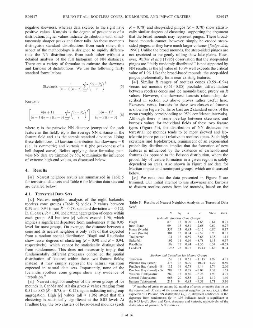
R = 0.78) and steep-sided pingos (R = 0.70) show statisti-cally similar degrees of clustering, supporting the argumentthat the broad mounds may represent pingos. These broad-based mounds cannot, however, simply be eroded steep-sided pingos, as they have much larger volumes [Sedgewick,1990]. Unlike the broad mounds, the steep-sided pingos arenot restricted to the gently rolling thaw-lake plains. How-ever, Walker et al.’s [1985] observation that the steep-sidedpingos are ‘‘fairly randomly distributed’’ is not supported byNN results, as the jcj value of 10.94 well exceeds the criticalvalue of 1.96. Like the broad-based mounds, the steep-sidedpingos preferentially form near existing features.[44] Similar R ranges of rootless cones (0.59–0.94)

versus ice mounds (0.51–0.85) precludes differentiationbetween rootless cones and ice mounds based purely on Rvalues. However, the skewness-kurtosis relationship de-scribed in section 3.3 above proves rather useful here.Skewness versus kurtosis for these two classes of featuresis shown in Figure 5a. Error bars are 2 standard errors of themean (roughly corresponding to 95% confidence intervals).Although there is some overlap between skewness andkurtosis values for individual fields of these two featuretypes (Figure 5b), the distribution of NN distances forterrestrial ice mounds tends to be more skewed and lep-tokurtic (more peaked) relative to rootless cones. Such highskewness and leptokurtosis, reminiscent of an exponentialprobability distribution, implies that the formation of newfeatures is influenced by the existence of earlier-formedfeatures (as opposed to the Poisson distribution, where theprobability of feature formation in a given region is solelydependent on area). Also shown in Figure 5 are data forMartian impact and nonimpact groups, which are discussedbelow.[45] We note that the data presented in Figure 5 are

trimmed. Our initial attempt to use skewness and kurtosisto discern rootless cones from ice mounds, based on the

Table 5. Results of Nearest Neighbor Analysis on Terrestrial Data

Setsa

N Nb R c Skew Kurt

Icelandic Rootless Cone GroupsBlagil 87 13 0.90 �1.68 0.64 0.21Innri Eyrar 69 13 0.81 �2.68 0.60 �0.27Hnuta (North) 357 13 0.83 �6.15 0.86 0.17Hnuta (South) 301 12 0.74 �8.52 0.90 0.31Trollhamar 131 12 0.59 �8.66 1.35 1.13Stakafell 192 11 0.66 �8.78 1.13 0.37Raudholar 198 17 0.94 �1.56 0.54 �0.53Landbrot 1282 23 0.77 �15.43 0.68 �0.04

Alaskan and Canadian Ice Mound GroupsTanacross 152 11 0.51 �11.15 1.99 4.31Prudhoe Bay (steep) 376 16 0.70 �10.94 1.22 0.80Prudhoe Bay (broad) - E 112 16 0.78 �4.14 1.74 2.90Prudhoe Bay (broad) - W 287 12 0.78 �7.02 1.32 1.63Western Tuktoyaktuk 282 13 0.80 �6.28 1.90 4.91Central Tuktoyaktuk 665 20 0.85 �7.31 1.17 1.60Eastern Tuktoyaktuk 213 9 0.83 �4.53 1.71 3.10

aN, number of cones or craters; Nb, number of cones or craters that lie onthe convex hull; R, ratio of the mean nearest neighbor distance (Ra) to thatexpected of a Poisson NN distribution (Re); c, statistical confidence in thedeparture from randomness (jcj > 1.96 indicates result is significant atthe 0.05 level); Skew and Kurt, skewness and kurtosis, respectively, of thedistribution of pairwise NN distances.


11 of 16

E06017

entire (i.e., untrimmed) NN distribution, yielded ambiguousresults. For rootless cones, kurtosis ranged from 2.89 to60.36 (mean kurtosis = 14.32; s = 19.39) and skewnessranged from 1.35 to 5.20 (mean skewness = 2.52, s = 1.20).The respective ranges for ice mounds are 3.49 to 39.85(mean kurtosis = 19.19, s = 14.85) and 1.82 to 5.31 (meanskewness = 3.56, s = 1.40). As the statistical distribution ofgeologic features reflects the physical processes that influ-enced feature formation [Bruno et al., 2004; Glaze et al.,2005], the NN distribution should bear some resemblance to

classical probability distributions such as those associatedwith random processes, population growth and resourceutilization. For comparison, the normal distribution hasskewness and kurtosis values each of zero; the exponentialdistribution has corresponding values of two and six,respectively. Other classical probability distributions gener-ally have similarly modest values of skewness and kurtosis.However, many of the feature fields included in thisanalysis have anomalously high values of skewness andkurtosis due to the influence of extreme high-end values.[46] Extreme values suggest that features have been

included in the data sets that belong to different statisticalpopulations and/or were formed under different physicalconditions. Visual inspection of the extreme values in thefeature fields included in this analysis suggests they tend tobe larger than average, and therefore may have caused amore pronounced depletion of local resources required forfeature formation. Alternatively, they may have formedduring different time periods, different ambient settings orby different physical processes that cannot be determined bya statistical analysis. Regardless, including extreme valuesinhibits our ability to distinguish feature types on the basisof skewness and kurtosis, as reflected in similar meanvalues and high standard deviations for rootless cones andice mounds. Consequently, we have investigated thesestatistics using trimmed NN distributions. Statistical trim-ming is a standard technique [e.g., Hoaglin et al., 1983] andis particularly useful in applications where influential fac-tors have not been completely eliminated or controlled, as isclearly the case in the spatial distribution of geologicalfeatures. We have found that excluding the highest 5% ofvalues yields a remarkable separation between terrestrial icemounds and rootless cones, and thus provides an importanttool for interpreting the Martian data sets.

4.2. Martian Impact Crater Groups

[47] Nearest neighbor results for the four Martian sec-ondary impact crater groups studied (Table 6) show Rvalues in the 1.04–1.20 range (�R = 1.12; s = 0.07). Theseresults indicate that the spacing between craters within thesecrater groups is, on average, 12% greater than would beexpected from a random distribution. Values of jcj rangefrom 0.65 to 4.49, with two of the four exceeding 1.96.Thus the spacing between craters, while always greater thanrandom, can only be significantly discerned from random-ness in two of the four cases.[48] Similarly, the two Martian pedestal crater groups

analyzed have R values of 1.00 and 1.07 (�R = 1.04; s =0.05). Both values of jcj are less than 1.96, so neither of thetwo spatial distributions can be statistically distinguishedfrom the Poisson NN distribution. Thus four of the siximpact crater groups have random distributions, as might beexpected from impact cratering processes. For the twogroups with greater-than-random NN separations, it isunclear whether the craters formed preferentially away fromexisting features, or whether subsequent modification (suchas crater obliteration) served to increase R.[49] Critically, none of the six crater impact groups

studied show any evidence of aggregation within a cratercluster (i.e., in all cases R � 1.00). Therefore they can beremotely distinguished from rootless cones and ice moundspurely on the basis of their degree of clustering (Figure 6).

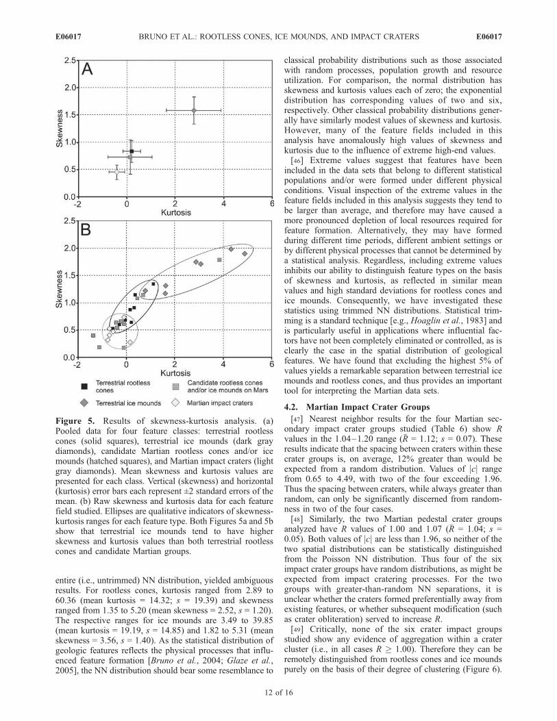
Figure 5. Results of skewness-kurtosis analysis. (a)Pooled data for four feature classes: terrestrial rootlesscones (solid squares), terrestrial ice mounds (dark graydiamonds), candidate Martian rootless cones and/or icemounds (hatched squares), and Martian impact craters (lightgray diamonds). Mean skewness and kurtosis values arepresented for each class. Vertical (skewness) and horizontal(kurtosis) error bars each represent ±2 standard errors of themean. (b) Raw skewness and kurtosis data for each featurefield studied. Ellipses are qualitative indicators of skewness-kurtosis ranges for each feature type. Both Figures 5a and 5bshow that terrestrial ice mounds tend to have higherskewness and kurtosis values than both terrestrial rootlesscones and candidate Martian groups.


12 of 16

E06017

This would be particularly useful for feature fields wheremorphology is not well-defined due to degradation, modi-fication, or sediment cover.

4.3. Martian Candidate Rootless Cone and/or IceMound Groups

[50] The ten candidate Martian groups studied have Rranging from 0.57 to 1.18 (�R = 0.81; s = 0.17). The onlyfeature field with R > 1.00 is found within Gusev Crater.Nearest neighbor results for these Gusev mounds (R = 1.18,c = 3.31) are markedly different from those of all othercandidate Martian groups, as well as from the terrestrialgroups of rootless cones and ice mounds. Unlike therootless cones and ice mounds, which tend to cluster neareach other, the Gusev mounds tend to form preferentiallyaway from preexisting features. This ‘‘repulsion’’ is signif-icantly different from random, as jcj exceeds 1.96. Nearestneighbor results for the Gusev mounds fall within the rangeof the Martian impact crater groups studied in terms of bothR (1.00–1.20) and c (0.07–4.49).[51] Excluding the Gusev mounds leaves an R range of

0.57–0.93 (�R = 0.77; s = 0.11), with all but one jcj valueexceeding 1.96. These values are nearly identical to thoseobtained for both the Icelandic rootless cones (�R = 0.78; s =0.12) and the terrestrial ice mounds (�R = 0.75; s = 0.12), yetshow no overlap with the R range of the Martian impactcrater groups studied (1.00–1.20). These NN results, sum-marized in Figure 6, lend support to the argument that thecandidate Martian groups (except the Gusev mounds) maybe rootless cones and/or ice mounds, but R and c valuesalone cannot be used to discriminate between these twopossible origins. Thus, as in section 4.1 above, we examinethe relationship between skewness and kurtosis.[52] Skewness and kurtosis values for both individual

feature fields and Mars candidate groups as a feature type

are shown in Figure 5, alongside the terrestrial data.Immediately apparent from Figure 5a is the strong overlapin the skewness-kurtosis relationship between the candidateMartian groups and the terrestrial rootless cones, althoughthe Martian data have more variance. The near coincidenceof the mean skewness and kurtosis values of these twogroups suggests they are drawing from the same population(i.e., that the candidate Martian groups are rootless cones).Detailed examination of the skewness-kurtosis relation ofindividual candidate Martian groups (Figure 5b; Table 6)reveals a somewhat more complex picture. One candidateMartian group (Cerberus Plains 1) has skewness and kur-tosis values falling well within the range of terrestrial icemounds. Two others (Cerberus Plains 2 and Isidis Planitia)have values intermediate between terrestrial rootless conesand ice mounds. Four groups (SE of Phlegra Montes N,Cerberus Plains 3, Athabasca Valles, and Acidalia Planitia)have skewness and kurtosis values well within the rootlesscone range. This result, together with the R and c values ofTable 6, suggests these four groups represent rootless cones.The same argument may hold for Amazonis Planitia and SEof Phlegra Montes (S), as their low skewness and kurtosisvalues suggest an ice mound origin is unlikely; howevertheir skewness and kurtosis values are lower than anyterrestrial rootless cone group. The final group (Gusev)has skewness and kurtosis values comparable to those ofMartian impact craters, which further suggests that thesemounds may represent modified impact craters (as dis-cussed below).

5. Discussion

5.1. Improved Methodology

[53] Using an improved NN methodology, we haveexamined the spatial distribution of rootless cones in Ice-

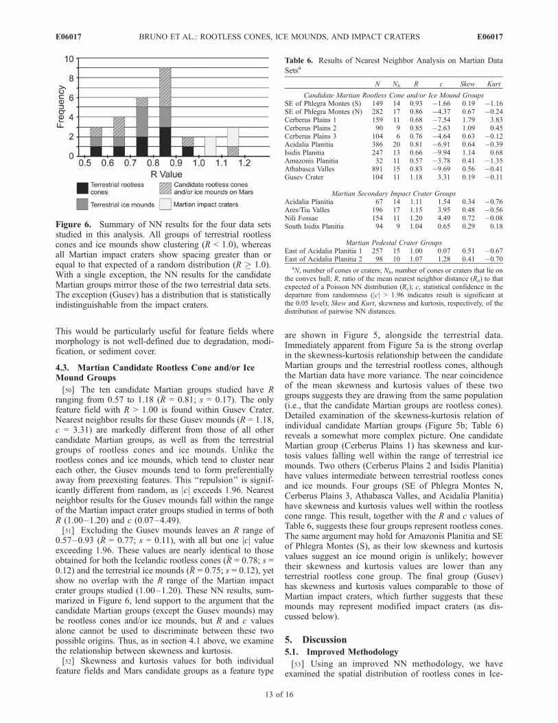
Figure 6. Summary of NN results for the four data setsstudied in this analysis. All groups of terrestrial rootlesscones and ice mounds show clustering (R < 1.0), whereasall Martian impact craters show spacing greater than orequal to that expected of a random distribution (R � 1.0).With a single exception, the NN results for the candidateMartian groups mirror those of the two terrestrial data sets.The exception (Gusev) has a distribution that is statisticallyindistinguishable from the impact craters.

Table 6. Results of Nearest Neighbor Analysis on Martian Data

Setsa

N Nb R c Skew Kurt

Candidate Martian Rootless Cone and/or Ice Mound GroupsSE of Phlegra Montes (S) 149 14 0.93 �1.66 0.19 �1.16SE of Phlegra Montes (N) 282 17 0.86 �4.37 0.67 �0.24Cerberus Plains 1 159 11 0.68 �7.54 1.79 3.83Cerberus Plains 2 90 9 0.85 �2.63 1.09 0.45Cerberus Plains 3 104 6 0.76 �4.64 0.63 �0.12Acidalia Planitia 386 20 0.81 �6.91 0.64 �0.39Isidis Planitia 247 13 0.66 �9.94 1.14 0.68Amazonis Planitia 32 11 0.57 �3.78 0.41 �1.35Athabasca Valles 891 15 0.83 �9.69 0.56 �0.41Gusev Crater 104 11 1.18 3.31 0.19 �0.11

Martian Secondary Impact Crater GroupsAcidalia Planitia 67 14 1.11 1.54 0.34 �0.76Ares/Tiu Valles 196 17 1.15 3.95 0.48 �0.56Nili Fossae 154 11 1.20 4.49 0.72 �0.08South Isidis Planitia 94 9 1.04 0.65 0.29 0.18

Martian Pedestal Crater GroupsEast of Acidalia Planitia 1 257 15 1.00 0.07 0.51 �0.67East of Acidalia Planitia 2 98 10 1.07 1.28 0.41 �0.70

aN, number of cones or craters; Nb, number of cones or craters that lie onthe convex hull; R, ratio of the mean nearest neighbor distance (Ra) to thatexpected of a Poisson NN distribution (Re); c, statistical confidence in thedeparture from randomness (jcj > 1.96 indicates result is significant atthe 0.05 level); Skew and Kurt, skewness and kurtosis, respectively, of thedistribution of pairwise NN distances.


13 of 16

E06017

land, ice mounds in Canada and Alaska, candidate rootlesscones and ice mounds on Mars, and pedestal and secondaryimpact craters on Mars. Our approach invokes four spatialstatistics (R, c, skewness, and kurtosis) and provides sys-tematic methods for defining the cluster boundary (i.e.,choosing a logical area and then constructing a convexhull) and treating border features (i.e., selectively excludingthose features that lie on the hull boundary). We have shownthat R and c values (the standard NN statistics) separateimpact craters from rootless cones and ice mounds, butsimilar degrees of clustering preclude differentiation be-tween the latter two feature types (Figure 6). This is wherethe skewness-kurtosis relation proves useful. The skewnessand kurtosis of the NN distribution provides a remarkablesegregation and grouping of terrestrial and Martian featuresfor a trivial amount of computation. What is most signifi-cant is that this segregation and grouping emerges withoutthe need for the postulation of an underlying probabilitydistribution.[54] The R values presented in this paper, on the basis of

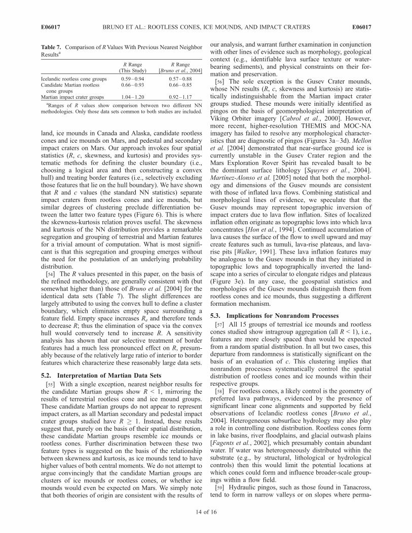
the refined methodology, are generally consistent with (butsomewhat higher than) those of Bruno et al. [2004] for theidentical data sets (Table 7). The slight differences arelargely attributed to using the convex hull to define a clusterboundary, which eliminates empty space surrounding afeature field. Empty space increases Re and therefore tendsto decrease R; thus the elimination of space via the convexhull would conversely tend to increase R. A sensitivityanalysis has shown that our selective treatment of borderfeatures had a much less pronounced effect on R, presum-ably because of the relatively large ratio of interior to borderfeatures which characterize these reasonably large data sets.

5.2. Interpretation of Martian Data Sets

[55] With a single exception, nearest neighbor results forthe candidate Martian groups show R < 1, mirroring theresults of terrestrial rootless cone and ice mound groups.These candidate Martian groups do not appear to representimpact craters, as all Martian secondary and pedestal impactcrater groups studied have R � 1. Instead, these resultssuggest that, purely on the basis of their spatial distribution,these candidate Martian groups resemble ice mounds orrootless cones. Further discrimination between these twofeature types is suggested on the basis of the relationshipbetween skewness and kurtosis, as ice mounds tend to havehigher values of both central moments. We do not attempt toargue convincingly that the candidate Martian groups areclusters of ice mounds or rootless cones, or whether icemounds would even be expected on Mars. We simply notethat both theories of origin are consistent with the results of

our analysis, and warrant further examination in conjunctionwith other lines of evidence such as morphology, geologicalcontext (e.g., identifiable lava surface texture or water-bearing sediments), and physical constraints on their for-mation and preservation.[56] The sole exception is the Gusev Crater mounds,

whose NN results (R, c, skewness and kurtosis) are statis-tically indistinguishable from the Martian impact cratergroups studied. These mounds were initially identified aspingos on the basis of geomorphological interpretation ofViking Orbiter imagery [Cabrol et al., 2000]. However,more recent, higher-resolution THEMIS and MOC-NAimagery has failed to resolve any morphological character-istics that are diagnostic of pingos (Figures 3a–3d). Mellonet al. [2004] demonstrated that near-surface ground ice iscurrently unstable in the Gusev Crater region and theMars Exploration Rover Spirit has revealed basalt to bethe dominant surface lithology [Squyres et al., 2004].Martınez-Alonso et al. [2005] noted that both the morphol-ogy and dimensions of the Gusev mounds are consistentwith those of inflated lava flows. Combining statistical andmorphological lines of evidence, we speculate that theGusev mounds may represent topographic inversion ofimpact craters due to lava flow inflation. Sites of localizedinflation often originate as topographic lows into which lavaconcentrates [Hon et al., 1994]. Continued accumulation oflava causes the surface of the flow to swell upward and maycreate features such as tumuli, lava-rise plateaus, and lava-rise pits [Walker, 1991]. These lava inflation features maybe analogous to the Gusev mounds in that they initiated intopographic lows and topographically inverted the land-scape into a series of circular to elongate ridges and plateaus(Figure 3e). In any case, the geospatial statistics andmorphologies of the Gusev mounds distinguish them fromrootless cones and ice mounds, thus suggesting a differentformation mechanism.

5.3. Implications for Nonrandom Processes

[57] All 15 groups of terrestrial ice mounds and rootlesscones studied show intragroup aggregation (all R < 1), i.e.,features are more closely spaced than would be expectedfrom a random spatial distribution. In all but two cases, thisdeparture from randomness is statistically significant on thebasis of an evaluation of c. This clustering implies thatnonrandom processes systematically control the spatialdistribution of rootless cones and ice mounds within theirrespective groups.[58] For rootless cones, a likely control is the geometry of

preferred lava pathways, evidenced by the presence ofsignificant linear cone alignments and supported by fieldobservations of Icelandic rootless cones [Bruno et al.,2004]. Heterogeneous subsurface hydrology may also playa role in controlling cone distribution. Rootless cones formin lake basins, river floodplains, and glacial outwash plains[Fagents et al., 2002], which presumably contain abundantwater. If water was heterogeneously distributed within thesubstrate (e.g., by structural, lithological or hydrologicalcontrols) then this would limit the potential locations atwhich cones could form and influence broader-scale group-ings within a flow field.[59] Hydraulic pingos, such as those found in Tanacross,

tend to form in narrow valleys or on slopes where perma-

Table 7. Comparison of RValues With Previous Nearest Neighbor

Resultsa

R Range(This Study)

R Range[Bruno et al., 2004]

Icelandic rootless cone groups 0.59–0.94 0.57–0.88Candidate Martian rootlesscone groups

0.66–0.93 0.66–0.85

Martian impact crater groups 1.04–1.20 0.92–1.17aRanges of R values show comparison between two different NN

methodologies. Only those data sets common to both studies are included.


14 of 16

E06017

frost is discontinuous or locally thinner. Thus a clustereddistribution may simply reflect preferred locations of dis-continuous or locally thinner permafrost. For hydrostaticpingos (e.g., Prudhoe Bay and Tuktoyaktuk Peninsula)which form following rapid drainage of lakes, a clustereddistribution could either reflect (1) a nonrandom distributionof thaw-lake basins (e.g., thaw-lake locations could becontrolled by the presence of drainage networks and drain-age barriers) and/or (2) a nonrandom process that affectswhich thaw-lakes are capable of generating pingos (e.g.,variable basin substrates may locally favor or prohibit thehydrological conditions required for pingo growth).

6. Conclusions

[60] We have shown that the spatial statistics of geologicfeatures can be an effective supplement to geologic contextand morphologic diagnostics to remotely differentiate be-tween feature types such as rootless cones, ice mounds, andimpact craters. Our method is based in part on the twostatistics of the conventional nearest neighbor approach, Rand c, which alone distinguish impact craters from the othertwo feature types. With a single exception, the R and cvalues of candidate Martian groups mirror those of terres-trial rootless cones and ice mounds. To further differentiatebetween these two feature types, we invoke the skewness-kurtosis relation, as ice mounds tend to have higher valuesof both central moments.[61] The skewness-kurtosis statistic generally favors a

rootless cone origin for the candidate Martian groups,although ice mounds remain a viable possibility forseveral groups. On the basis of NN results (as well asmorphology), these Martian groups are clearly not clustersof impact craters: impact craters have distinctly differentspatial distributions. The sole exception is the GusevCrater mounds, which have R, c, skewness, and kurtosisvalues that are indistinguishable from those of Martianimpact craters.[62] In summary, we have developed an improved method

for characterizing the spatial distribution of candidate root-less cones and ice mounds on Mars and quantitativelycomparing them with terrestrial analogs. These results pro-vide a basis for detailed physical modeling of the processesthat form fields of these features and wider systematicapplications may provide improvements in our understand-ing of the volatile inventory and evolution on Mars.

Notation

c statistical measure of confidence in the departure fromrandomness.

n number of features in the feature field.r distance between a feature and its nearest neighbor,

[L].R statistical measure of departure from randomness of

spatial distribution, = Ra/Re.�R average R value (for multiple feature fields).Ra average distance between nearest neighbors, [L].Re average nearest neighbor spacing expected for a

spatially random distribution [L].s sample standard deviation [L].r spatial density of features within a field, [L�2].

sRestandard error of the mean of nearest neighbordistances in a randomly distributed population [L].

[63] Acknowledgments. We thank all those who shared their knowl-edge and provided insights, including T. Thordarson (rootless cones andlava inflation), E. Pilger (programming), and S. Still (clustering). Thoroughreviews by L. Glaze and P. Lanagan led to significant improvements in thismanuscript. This work was supported in part by NASA Mars Data AnalysisProgram grant NAG5-13458 to S.A.F. This paper is HIGP contribution1436 and SOEST contribution 6774.

ReferencesAllen, C. C. (1979a), Volcano-ice interactions on Mars, J. Geophys. Res.,84, 8048–8059.

Allen, C. C. (1979b), Volcano-ice interactions on the Earth and Mars, Ph.D.thesis, 131 pp, Univ. of Arizona, Tucson.

Barlow, N. G., J. M. Boyce, F. M. Costard, R. A. Craddock, J. B. Garvin,S. E. H. Sakimoto, R. O. Kuzmin, D. J. Roddy, and L. A. Soderblom(2000), Standardizing the nomenclature of Martian impact cratermorphologies, J. Geophys. Res., 105, 26,733–26,738.

Barnouin-Jha, O. S., and P. H. Schultz (1996), Ejecta entrainment by im-pact-generated ring vortices: Theory and experiments, J. Geophys. Res.,101, 21,099–21,115.

Barnouin-Jha, O. S., and P. H. Schultz (1998), Lobateness of impact ejectadeposits from atmospheric interactions, J. Geophys. Res., 103, 25,739–25,756.

Brockett, B. E. (1982), Modification of and experience with a portable drill,Prudhoe Bay, Alaska, spring 1982, 14 pp., memorandum, Cold RegionsRes. and Eng. Lab., U.S. Army Corps of Eng., Hanover, N. H.

Bruno, B. C., S. A. Fagents, T. Thordarson, S. M. Baloga, and E. Pilger(2004), Clustering within rootless cone groups on Iceland and Mars:Effect of nonrandom processes, J. Geophys. Res., 109, E07009,doi:10.1029/2004JE002273.

Burr, D. M., J. A. Grier, A. S. McEwen, and L. P. Keszthelyi (2002a),Repeated aqueous flooding from the Cerberus Fossae: Evidence for veryrecently extant, deep groundwater on Mars, Icarus, 159, 53–73.

Burr, D. M., A. S. McEwen, and S. E. H. Sakimoto (2002b), Recent aqu-eous floods from the Cerberus Fossae, Mars, Geophys. Res. Lett., 29(1),1013, doi:10.1029/2001GL013345.

Burr, D. M., R. J. Soare, and J.-M. Wan Bun Tseung (2005), Young (lateAmazonian), near surface, ground ice features near the equator, Athabas-ca Valles, Mars, Icarus, 178, 56–73.

Cabrol, N. A., E. A. Grin, and W. H. Pollard (2000), Possible frost moundsin an ancient Martian lake bed, Icarus, 145, 91–107.

Carr, M. H. (1981), The Surface of Mars, 232 pp., Yale Univ. Press, NewHaven, Conn.

Carr, M. H., L. S. Crumpler, J. A. Cutts, R. Greeley, J. E. Guest, andH. Masursky (1977), Martian impact craters and emplacement of ejectaby surface flow, J. Geophys. Res., 82, 4055–4065.

Carr, M. J. (1976), Underthrusting and Quaternary faulting in northernCentral America, Geol. Soc. Am. Bull., 87, 825–829.

Chapman, M. G., and K. L. Tanaka (2001), Interior trough deposits onMars: Subice volcanoes?, J. Geophys. Res., 106, 10,087–10,100.

Clark, P. J., and F. C. Evans (1954), Distance to nearest neighbor as ameasure of spatial relationships in populations, Ecology, 35, 445–453.

Connor, C. B. (1990), Cinder cone clustering in the TransMexican volcanicbelt: Implications for structural and petrologic models, J. Geophys. Res.,95, 19,395–19,405.

Connor, C. B., and B. E. Hill (1995), Three nonhomogeneous Poissonmodels for the probability of basaltic volcanism: Application to the YuccaMountain region, Nevada, J. Geophys. Res., 100, 10,107–10,125.

Connor, C. B., C. D. Condit, L. S. Crumpler, and J. C. Aubele (1992),Evidence of regional structural controls on vent distribution: Springer-ville Volcanic Field, Arizona, J. Geophys. Res., 97, 12,349–12,359.

Fagents, S. A., and T. Thordarson (2006), Rootless volcanic cones in Ice-land and on Mars, in The Geology of Mars: Evidence From Earth-BasedAnalogues, edited by M. G. Chapman and I. P. Skilling, Cambridge Univ.Press, New York, in press.

Fagents, S. A., P. D. Lanagan, and R. Greeley (2002), Rootless coneson Mars: A consequence of lava-ground ice interaction, in Volcano-IceInteraction on Earth and Mars, edited by J. L. Smellie and M. G.Chapman, Geol. Soc. Spec. Publ., 202, 295–317.

Farrand, W. H., L. R. Gaddis, and L. Keszthelyi (2005), Pitted cones anddomes on Mars: Observations in Acidalia Planitia and Cydonia Mensaeusing MOC, THEMIS, and TES data, J. Geophys. Res., 110, E05005,doi:10.1029/2004JE002297.

Frey, H., and M. Jarosewich (1982), Subkilometer Martian volcanoes:Properties and possible terrestrial analogs, J. Geophys. Res., 87, 9867–9879.


15 of 16

E06017

Frey, H., B. L. Lowry, and S. A. Chase (1979), Pseudocraters on Mars,J. Geophys. Res., 84, 8075–8086.

Gaidos, E., and G. Marion (2003), Geological and geochemical legacy of acold early Mars, J. Geophys. Res., 108(E6), 5055, doi:10.1029/2002JE002000.

Gault, D. E., and R. Greeley (1978), Exploratory experiments of impactcraters formed in viscous-liquid targets: Analogs for Martian rampartcraters?, Icarus, 34, 486–495.

Glaze, L. S., S. W. Anderson, E. R. Stofan, S. Baloga, and S. E. Smrekar(2005), Statistical distribution of tumuli on pahoehoe flow surfaces:Analysis of examples in Hawaii and Iceland and potential applicationsto lava flows on Mars, J. Geophys. Res., 110, B08202, doi:10.1029/2004JB003564.

Graham, R. (1972), An efficient algorithm for determining the convex hullof a finite planar point set, Info. Proc. Lett., 1, 132–133.

Greeley, R., and S. A. Fagents (2001), Icelandic pseudocraters as analogsto some volcanic cones on Mars, J. Geophys. Res., 106, 20,527–20,546.

Grizzaffi, P., and P. H. Schultz (1989), Isidis Basin: Site of ancient volatile-rich debris layer, Icarus, 77, 358–381.

Hasenaka, T., and I. S. E. Carmichael (1985a), The cinder cones ofMichoacan-Guanajuato, central Mexico: Their age, volume, distributionand magma discharge rate, J. Volcanol. Geotherm. Res., 25, 105–124.

Hasenaka, T., and I. S. E. Carmichael (1985b), A compilation of location,size and geomorphological parameters of volcanoes in the Michoacan-Guanajuato volcanic field, Mexico, Geofis. Int., 24, 577–608.

Heming, R. F. (1980), Patterns of Quaternary basaltic volcanism in thenorthern North Island, New Zealand, N. Z. J. Geol. Geophys., 23,335–344.

Hoaglin, D. C., F. Mosteller, and J. W. Tukey (1983), UnderstandingRobust and Exploratory Data Analysis, 447 pp., John Wiley, Hoboken,N. J.

Holmes, G., D. Hopkins, and H. Foster (1968), Pingos in Central Alaska,40 pp., Geol, Surv. Bull. 1241-H, U.S. Dept. of the Interior, Washington,D. C.

Hon, K., J. Kauahikaua, R. Denlinger, and K. Mackay (1994), Emplace-ment and inflation of pahoehoe sheet flows: Observations and measure-ments of active lava flows on Kilauea Volcano, Hawaii, Geol. Soc. Am.Bull., 106, 351–370.

Lanagan, P. D., A. S. McEwen, L. P. Keszthelyi, and T. Thordarson (2001),Rootless cones on Mars indicating the presence of shallow equatorialground ice in recent times, Geophys. Res. Lett., 28, 2365–2368.

Lucchitta, B. K. (1981), Mars and Earth: Comparison of cold climatefeatures, Icarus, 45, 264–303.

Mackay, J. R. (1962), Pingos of the Pleistocene Mackenzie Delta area,Geogr. Bull. 18, pp. 21–63, Geogr. Branch, Mines and Tech. Surv.,Ottawa, Canada.

Mackay, J. R. (1973), The growth of pingos, western Arctic coast, Canada,Can. J. Earth Sci., 10, 979–1004.

Mackay, J. R. (1979), Pingos of the Tuktoyaktuk Peninsula area, NorthwestTerritories, Geogr. Phys. Quat., 33, 3–61.

Mackay, J. R. (1987), Some mechanical aspects of pingo growth and fail-ure, western Arctic coast, Canada, Can. J. Earth Sci., 24, 1108–1119.

Mackay, J. R. (1998), Pingo growth and collapse, Tuktoyaktuk PeninsulaArea, western Arctic coast, Canada: A long-term field study, Geogr. Phys.Quat., 52, 271–323.

Martınez-Alonso, S., B. M. Jakosky, M. T. Mellon, and N. E. Putzig (2005),A volcanic interpretation of Gusev Crater surface materials from thermo-physical, spectral, and morphological evidence, J. Geophys. Res., 110,E01003, doi:10.1029/2004JE002327.

Mellon, M. T., W. C. Feldman, and T. H. Prettyman (2004), The presenceand stability of ground ice in the southern hemisphere of Mars, Icarus,169, 324–340.

Mouginis-Mark, P. J. (1987), Water or ice in the Martian regolith?: Cluesfrom rampart craters seen at very high resolution, Icarus, 71, 268–286.

Muller, F. (1959), Meddeleser on Grønland (in German), 153(3), 127 pp.(translated by D. A. Sinclair, Natl. Res. Counc. of Can, Ottawa, Ont., 117pp., 1963).

Oskarsson, B. V. (2005), Lava-rise structures in pahoehoe and aa: Examplesfrom the Hrutagja lava shield and Kapelluhraun aa flow field on theReykjanes Peninsula, B.Sc. thesis, Univ. of Iceland, Reykjavik.

Page, D. P., and J. B. Murray (2006), Stratigraphic and morphologicalevidence for pingo genesis in the Cerberus plains, Icarus, doi:10.1016/j.icarus.2006.01.017, in press.

Parker, T. J., D. S. Gorsline, R. S. Saunders, D. C. Pieri, and D. M.Schneeberger (1993), Coastal geomorphology of the Martian northernplains, J. Geophys. Res., 98, 11,061–11,078.

Plescia, J. B. (1990), Recent flood lavas in the Elysium region of Mars,Icarus, 88, 465–490.

Plescia, J. B. (1993), An assessment of volatile release from recent volcan-ism in Elysium, Mars, Icarus, 104, 20–32.

Plescia, J. B. (2003), Cerbereus Fossae, Elysium, Mars: A source of lavaand water, Icarus, 164, 79–95.

Porsild, A. E. (1938), Earth mounds in unglaciated Arctic northwesternAmerica, Geogr. Rev., 28, 46–58.

Rossbacher, L. A., and S. Judson (1981), Ground ice on Mars; inventory,distribution, and resulting landforms, Icarus, 45, 39–59.

Schultz, P. H. (1992), Atmospheric effects on ejecta emplacement, J. Geo-phys. Res., 97, 11,623–11,662.

Schultz, P. H., and D. E. Gault (1979), Atmospheric effects on Martianejecta emplacement, J. Geophys. Res., 84, 7669–7687.

Sedgewick, R. (1990), Algorithms in C, 657 pp., Addison-Wesley Long-man, Boston, Mass.

Settle, M. (1979), The structure and emplacement of cinder cone fields, Am.J. Sci., 279, 1089–1107.

Soare, R. J., D. M. Burr, and J.-M. Wan Bun Tseung (2005), Possiblepingos and a periglacial landscape in northwest Utopia Planitia, Icarus,174, 373–382, doi:310.1016/j.icarus.2004.1011.1013.

Squyres, S. W., S. M. Clifford, R. O. Kuzmin, J. R. Zimbelman, and F. M.Costard (1992), Ice in the Martian regolith, in Mars, edited by H. H.Kieffer et al., pp. 523–554, Univ. of Ariz. Press, Tucson.

Squyres, S. W., C. Howell, M. C. Liu, and J. J. Lissauer (1997), Investiga-tion of crater ‘saturation’ using spatial statistics, Icarus, 125, 67–82.

Squyres, S. W., et al. (2004), The Spirit Rover’s Athena science investiga-tion at Gusev crater, Mars, Science, 305, 794–799.

Stager, J. K. (1956), Progress report on the analysis of the characteristicsand distribution of pingos east of the Mackenzie delta, Can. Geogr., 7,13–20.

Tanaka, K. L. (1997), Sedimentary history and mass flow structures ofChryse and Acidalia Planitiae, Mars, J. Geophys. Res., 102, 4131–4419.

Theilig, E., and R. Greeley (1979), Plains and channels in the Lunae Pla-num–Chryse Planitia region of Mars, J. Geophys. Res., 84, 7994–8010.

Thorarinsson, S. (1951), Laxargljufur and Laxarhraun. A tephrochronolo-gical study, Geogr. Ann., H1–2, 1–89.

Thorarinsson, S. (1953), The crater groups in Iceland, Bull. Volcanol., 14,3–44.

Thordarson, T. (2000), Rootless eruptions and cone groups in Iceland:Products of authentic explosive water to magma interactions, in Volca-no/Ice Interactions on Earth and Mars, Abstract Volume, edited by V. C.Gulick and M. T. Gudmundsson, p. 48, Univ. of Iceland, Reykjavik.

Thordarson, T., and A. Hoskuldsson (2002), Iceland, Terra, Harpenden,Hertfordshire, U. K.

Thordarson, T., D. J. Miller, and G. Larsen (1998), New data on theLeidolfsfell cone group on south Iceland, Jokull, 46, 3–15.

Thordarson, T., M. M. Morrissey, G. Larsen, and H. Cyrusson (1992),Origins of rootless cone complexes in S. Iceland, in The 20th NordicGeological Winter Meeting, edited by A. Geirsdottir, H. Norddahl, andG. Helgadottir, p. 169, Icelandic Geol. Soc., Reykjavik.

Thoroddsen, T. (1894), Ferd un Vestur Skaftafellssyslu sumarid 1893 (Tra-velogue from Western Skaftafellshire in the summer of 1893), Andvari,19, 44–161.

Walker, D., M. Walker, K. Everett, and P. Webber (1985), Pingos of thePrudhoe Bay Region, Alaska, Arctic Alpine Res., 17, 321–336.

Walker, G. P. L. (1991), Structure, and origin by injection of lava undersurface crust, of tumuli, ‘‘lava rises’’, ‘‘lava rise pits’’, and lava inflationclefts in Hawaii, Bull. Volcanol., 53, 546–558.

Walker, J. (1981), Petrogenesis of lavas from cinder cone fields behind thevolcanic front of Central America, J. Geol., 89, 721–739.

Washburn, A. L. (1973), Periglacial Processes and Environments, 320 pp.,Edward Arnold, London.

��S. M. Baloga, Proxemy Research, 20528 Farcroft Lane, Bowie, MD

20882, USA.B. C. Bruno, S. A. Fagents, and C. W. Hamilton, Hawai i Institute of

Geophysics and Planetology, University of Hawai`i, 1680 East WestRoad,POST 504, Honolulu, HI 96822, USA. ([email protected])D. M. Burr, SETI Institute, 515 North Whisman Road, Mountain View,

CA 94043, USA.


16 of 16

E06017

Documents

Identification of volcanic rootless cones, ice mounds, and