DESY 17-096

Enabling rootless Linux Containers in multi-user

environments: the udocker tool

Jorge Gomes1, Emanuele Bagnaschi2, Isabel Campos3,Mario David1, Luıs Alves1, Joao Martins1, Joao Pina1, Alvaro Lopez-Garcıa3, and

Pablo Orviz3

1Laboratorio de Instrumentacao e Fısica Experimental de Partıculas (LIP), Lisboa,Portugal

2Deutsches Elektronen-Synchrotron (DESY), 22607 Hamburg, Germany3IFCA, Consejo Superior de Investigaciones Cientıficas-CSIC, Santander, Spain

November 7, 2017

Abstract

Containers are increasingly used as means to distribute and run Linuxservices and applications. In this paper we describe the architecturaldesign and implementation of udocker a tool to execute Linux containersin user mode and we describe a few practical applications for a range ofscientific codes meeting different requirements: from single core executionto MPI parallel execution and execution on GPGPUs.

1 Introduction

Technologies based on Linux containers have become very popular among soft-ware developers and system administrators. The main reason behind this suc-cess is the flexibility and efficiency that containers offer when it comes to pack,deploy and run software. A containerized version of a given software can be cre-ated including all its dependencies, so that can be executed seamlessly regardlessof the Linux distribution in the target hosts.

From the point of view of virtualization itself containers provide a lightweightoperating-system-level virtualization. This is achieved by using advanced fea-tures of modern Linux kernels [1], namely control groups and namespaces isola-tion [2, 3]. Using both features a group of processes can be contained in a fullyisolated environment (using namespace isolation), with a fixed/defined amountof resources such as CPU or RAM allocated to them (using control groups).This encapsulated group of processes is what we call container.

Since containers run using the kernel of the host machine, they do not needto boot their own operating system. Therefore they can be seen as a lightweightapproach to virtualization, when compared with conventional Virtual Machines

1

arX

iv:1

711.

0175

8v1

[cs

.SE

] 6

Nov

201

7

(VM) such as the ones provided using para-virtualization or hardware virtualmachines.

In particular a given machine may host many more containers than virtualmachines, as the first ones occupy less hardware resources (notably memory).Also, transferring, starting and shutting down containers is usually much fasterthan performing the same operations on a conventional virtual machine.

The idea of operating-system-level virtualization is not new. The first at-tempts can be traced back to the chroot system call (introduced in 1979), whichenables changing the root directory for a given process and its children. Theconcept was later extended in the jailed systems of BSD [4] (released in 1998).However the developments needed at the level of the Linux kernel to make ithappen in a consistent and robust way have taken a few years to crystallise.The Control groups technology, also known as cgroups, is present in the Linuxkernels since version 2.6.24 (released in 2008). Support for namespaces wasfirst introduced in the Linux kernel 2.4.19 (released in 2002), with additionalnamespaces and enhancements being added since.

On the side of the tools needed to implement containers, the LXC [5] tool-kit (initially released in 2008) was the first comprehensive implementation totake advantage of cgroups and namespaces to provide isolated execution envi-ronments in Linux. Still the use of LXC requires considerable knowledge and itwas with Docker [6] that Linux Containers gained wide adoption.

Docker introduced a simple interface to create, distribute and execute Linuxcontainers. The first versions of Docker made use of LXC as a means to setupand execute containers. Using Docker is possible to provide multiple, isolatedLinux environments, running on the same host machine, in a very flexible anduser friendly manner. In this respect Docker is being very successful in enablingnot only containerized services but also applications. Besides providing thetools to build the images and execute them, it provides a high-level API whichallows interacting in a simple way with a catalogue of pre-defined or self-madecontainers (the Dockerhub [7]). Docker makes use of a layered filesystem whichprovides the advantage of saving storage space and minimize downloads bysharing common layers across containers. The usage of a layered filesystemmakes containers more robust in front of data losses, and less prone to writingmistakes on the underlying layers.

However Docker presents limitations specially when it comes to deploy con-tainers in multi-user systems. In Docker, processes within the container arenormally executed as root below the Docker daemon process tree, thus escapingto the resource usage policies, accounting controls, and process controls thatare imposed to normal users. Docker is usually unavailable in multi-user sys-tems due both to these limitations and to security concerns of allowing users tocontrol Docker and through it achieve privileged access to the host system.

Unfortunately most scientific computing resources such as High PerformanceComputing (HPC) systems, Linux clusters or grid infrastructures are multi-user systems and fall in this category. Therefore the adoption of Docker inthis type of infrastructures has been limited. This fact seriously hampers theapplicability of Docker for scientific computing and has lead to the development

2

of other solutions such as Singularity [8] or Shifter [9]. These solutions are notcompatible with Docker, require installation by the system administrator andprivileges to setup or execute also limiting their adoption.

Another limitation of Docker is support for execution of parallel applicationsthat require network communication across multiple hosts. For security reasonsDocker containers are executed with network namespaces making direct com-munication between containers across hosts more difficult. The use of networknamespaces can be disabled but creates security concerns as processes withinthe container running as root may access the host sockets. Similarly access tohost devices from within the container can also raise security issues.

The performance of the Docker layered filesystem is in general slower thanaccessing the host filesystem directly. Also any write operation in the layeredfilesystem can only happen by adding another layer on top of the existing ones.As layers are immutable files in underlying layers can be hidden but cannotbe deleted making the container images grow in time. Containers build forcomplex scientific applications like the ones we describe as example grow up toa few Gigabytes, therefore the question of accessibility and disk space becomesalso a point of concern. Therefore containers need to be constantly regeneratedfrom scratch to keep their size manageable.

In this work we address the problematic of executing Docker containers inuser space, i.e. without installing additional system software, without requiringany administrative privileges and in a way that respects resource usage policies,accounting and process controls. Our aim is to empower users to execute appli-cations encapsulated in Docker containers easily in any Linux system includingcomputing clusters regardless of Docker being locally available.

In section 2 we will describe the architectural elements of the tool we havedeveloped to address the above mentioned problems and shortfalls. The re-maining of the paper is devoted to describe the practical applicability of thismiddleware. We describe how such solution can be applied by users of threevery different use cases which we believe are representative enough of the currentscientific computing landscape.

The first use case describes an application highly complex in the sense oflibrary dependences, legacy code, and software dependencies. The second caseaddresses the usage of containers in MPI parallel applications using Infinibandand/or TCP/IP. Finally we also show how to target specialized hardware accel-erators such as GPGPUs.

All the tools presented here are open-source and may be downloaded fromour public repository [10].

2 Architectural design

To overcome the limitations mentioned in section 1 we have explored the possi-bilities available to run applications encapsulated in Docker containers in userspace in a portable way. Our technical analysis is as follows.

3

2.1 Technical Analysis

Most scientific applications do not require the full set of Docker features. Theseapplications are usually developed to be executed in multi-user shared environ-ments by unprivileged users. Therefore features such as isolation are not strictlyneeded as long as the applications are executed without privileges. The funda-mental features that make Docker appealing as a means to execute scientificapplications are thus the following:

• the ability to provide a separate directory tree where the application withall its dependencies can execute independently from the target host;

• possibility of mounting host directories inside the container directory tree,which is convenient for data access;

• easy software packaging with Dockerfiles;

• reuse of previously created images;

• easy sharing and distribution of images via Docker repositories such asDocker Hub and many others;

• simple command line and REST interfaces.

Several of these features such as creating containers and pushing them intorepositories can be accomplished from the user desktop or portable computerusing Docker directly. Therefore we assume that Docker can be used to preparethe containers and that the focus should rather be put on enabling the executionof the created containers in systems where Docker is unavailable.

The most complex aspect is to provide a chroot-like functionality so thatDocker containers can be executed without conflicting with the host operatingsystem environment. The chroot system call requires privileges and thereforewould collide with our objective of having a tool that would not require privilegesor installation by the system administrator. Three alternative approaches toimplement chroot-like functionality without privileges were identified:

• use unprivileged User Namespaces;

• use PTRACE to intercept calls that handle pathnames;

• use LD PRELOAD to intercept calls that handle pathnames.

The use of unprivileged User Namespaces allows a non-privileged user totake advantage of the Linux namespaces mechanism. This approach is onlyusable since kernel 3.19. Unfortunately the implementation of unprivileged User

Namespaces exposes the processes running inside the container to limitationsespecially in terms of mappings of group identifiers. Furthermore this approachdoes not work on certain distributions such as CentOS 6 and CentOS 7, whichdo not provide kernels having the necessary features. Due to these limitationsthis approach was initially discarded.

4

The PTRACE mechanism enables tracing of system calls making possible tochange their calling parameters in run time. System calls that use pathnamescan be traced and dynamically changed so that references to pathnames withinthe container can be dynamically expanded into host pathnames prior to thesystem calls and upon their return. The biggest drawback of using PTRACE toimplement chroot-like functionality is the impact on performance. An externalprocess needs to trace the execution of the application, stop it before each systemcall, change its parameters when they reference pathnames, and continue fromthe same point. If the system call returns pathnames a second stop must beperformed when the call returns to perform the required changes. In olderkernels (such as in CentOS 6) all system calls need to be traced. In morerecent kernels is possible to use PTRACE with SECCOMP filtering to performselective system call tracing thus allowing to restrict interception only to theset of calls that manipulate pathnames. The impact of using PTRACE dependson the availability of SECCOMP and on how frequently the application invokessystem calls.

The LD PRELOAD mechanism allows overriding of shared libraries. Inpractice this approach allows to call wrapping functions where the pathnamescan be changed before and after invoking the actual system functions. TheLD PRELOAD mechanism is implemented by the dynamic loader ld.so. Thedynamic loader is an executable that finds and loads shared libraries and pre-pares programs for execution. The dynamic loader also provides a set of callsthat enable applications to load further dynamic libraries in run time. When ashared library pathname does not contain a slash the dynamic loader searchesfor the library in the directory locations provided by:

• DT RPATH dynamic section attribute of the ELF executable;

• LD LIBRARY PATH environment variable;

• DT RUNPATH dynamic section attribute of the ELF executable;

• cache file /etc/ld.so.cache;

• default paths such as /lib64, /usr/lib64, /lib, /usr/lib.

Due to this behaviour, libraries from the host system may end-up beingloaded instead of the libraries within the chroot-environment. Furthermore thefollowing limitations apply:

• this approach depends on dynamic linking and does not work with stati-cally linked executables;

• the absolute pathname to the dynamic loader is encoded in the executa-bles, leading to the invocation of the host dynamic loader instead of thedynamic loader provided in the container;

• dynamic executables and shared libraries may also reference other sharedlibraries, if they have absolute pathnames then they may be loaded fromlocations outside of the container.

5

2.2 The udocker tool

To validate the concept we developed a tool called udocker that combinesthe pulling, extraction and execution of Docker containers without privileges.udocker is an integration tool that incorporates several execution methods giv-ing the user the best possible options to execute their containers according to thetarget host capabilities. udocker is written in Python and aims to be portable.udocker has eight main blocks:

• user command line interface;

• self installation;

• interface with Docker Hub repositories;

• local repository of images;

• creation of containers from images;

• local repository of containers;

• containers execution;

• specific execution methods.

udocker provides a command line interface similar to Docker and provides asubset of its commands aimed at searching, pulling and executing containers ina Docker like manner.

The self installation allows a user to transfer the udocker Python scriptand upon the first invocation pull any additional required tools and librarieswhich are then stored in the user directory. This allows udocker to be easilydeployed and upgraded by the user himself. udocker can also be installed froma previously downloaded tarball.

The Docker images are composed of filesystem layers. Each layer has meta-data and a directory tree that must be stacked by the layered filesystem toobtain the complete image. The Docker layered filesystem is based on UnionFS[11]. In UnionFS file deletion is implemented by signalling the hiding of files inthe lower layers via additional files that act as markers white-outs. We thereforeimplemented the pulling of images by downloading the corresponding layers andmetadata using the Docker Hub REST API. A simple repository has been im-plemented where layers and metadata are stored. Layers are shared across theimages to save space. The repository is by default placed in the user home di-rectory. To prepare a container directory tree, the several layers are sequentiallyextracted over the previous ones respecting the white-outs. File protections arethen adjusted so that the user can access all container files and directories. Thecontainer directory tree is also stored in the local repository. The containerexecution is achieved with a chroot-like operation using the previously preparedcontainer directory tree.

6

udocker implements the parsing of Docker container metadata and supportsa subset of metadata options namely: the command to be invoked when thecontainer is started, mount of host directories, setting of environment variables,and the initial working directory.

The PTRACE execution method was implemented using PRoot [12], a toolthat provides chroot-like functionality using PTRACE. PRoot also providesmapping of host files and directories into the container enabling access fromthe container to host locations. We had to develop fixes for PROOT to makeSECCOMP filtering work together with PTRACE due to changes introducedin the Linux kernel 3.8 and above. A fix for proper clean-up of temporary fileswas also added.

The LD PRELOAD method is based on Fakechroot [13] a library that pro-vides chroot-like functionality using this mechanism, and is commonly used inDebian to install a base system in a subdirectory. Fakechroot provides mostof the wrapping functions that are needed. However due to the previously de-scribed behaviour of the dynamic loader, applications running under Fakechrootmay unwillingly load shared libraries from the host. udocker implements severalstrategies to address these shortcomings.

• Replacement of the dynamic loader pathname in the executables header,thus forcing the execution of the loader provided with the container.

• Replacement of DT RPATH and DT RUNPATH in the executables, forc-ing the search paths to container locations.

• Replacement of shared library names within the headers of executablesand libraries, forcing them to container locations.

• Extraction of shared libraries pathnames from ld.so.cache which are thenmodified and added to LD LIBRARY PATH.

• Interception of changes to LD LIBRARY PATH forcing the paths to con-tainer locations.

• Prevent the dynamic loader from accessing the host ld.so.cache

• Prevent the dynamic loader from loading libraries from the host /lib64,/usr/lib64, /lib, /usr/lib.

Changes to executables and libraries are performed using PatchELF [14].PatchELF was enhanced to manage the pathname prefixes of: the dynamicloader within executables, library dependencies and their paths in executablesand shared libraries. The ld.so executable within the container can also bemodified by udocker to prevent the loading of shared libraries from the host.All the above changes are performed automatically by udocker depending onthe execution mode selected. The Fakechroot library was heavily modified toaddress multiple limitations, change executables and libraries in run time, andto provide better mapping of host directories and files inside the container.

7

The support for unprivileged User Namespaces and rootless containers wasimplemented using runC [15], a tool for spawning and running containers accord-ing to the Open Containers Initiative OCI [16] specification. udocker translatesDocker metadata and the command line arguments to build a matching OCIconfiguration spec that enables the container execution in unprivileged mode.

All external tools including PRoot, PatchELF, runC and Fakechroot areprovided together with udocker. The binary executables are statically com-piled to be used across multiple Linux distributions unchanged and increasingportability. udocker itself has a minimal set of Python dependencies and canbe executed in a wide range of Linux systems. udocker can be either deployedand managed entirely by the end-user or centrally deployed by a system admin-istrator. The udocker execution takes place under the regular userid withoutrequiring any additional privilege.

3 Description of Basic Capabilities

In this section we provide a description of the main capabilities of udocker.As previously stated, it mimics a subset of the Docker syntax to facilitate itsadoption and use by those already familiar with Docker tools. As pointed outin sections 1 and 2, it does not make use of Docker nor requires its presence.The current implementation is limited to the pulling and execution of Dockercontainers. The actual containers should be built using Docker and Dockerfiles.udocker does not provide all the Docker features since it’s not intended as aDocker replacement but oriented to providing a run-time environment for con-tainers execution in user space. The following is a list of examples, see [10] fora complete list.

• Pulling containers from Docker Hub or from private Docker repositories.

udocker pull docker.io/repo_name/container_name

The image of the container with its layers is downloaded to the directoryspecified by the user. The location of that directory is controlled by anenvironment variable $UDOCKER DIR that can be defined by the user. Itshould point to a directory in a filesystem where there is enough capacityto unroll the image. The default location is $HOME/.udocker.

• Once the image is downloaded, the container directory tree can be ob-tained from the container layers using the option create.

Upon exit udocker displays the identifier of the newly created container,a more understandable name can be associated to the container identifierusing the option name. In the example below, the content of the ROOT

directory of a given container is shown. The ROOT is a subdirectory belowthe container directory.

8

$shell> udocker create docker.io/repo_name/container_name

95c22b84-1868-332b-9bf0-2e056beafb00

$shell> udocker name 95c22b84-1868-332b-9bf0-2e056beafb00 \

my_container

$shell> ls $HOME/.udocker

bin containers layers lib repos

$shell> ls .udocker/containers/my_container/ROOT/

bin dev home lib64 media opt root sbin sys usr

boot etc lib lost+found mnt proc run srv tmp var

• Install software inside the container.

udocker run --user=root container_name \

yum install -y firefox pulseaudio gnash-plugin

In this example we used the capability to partially emulate root in order touse yum to install software packages in the container. No root privileges areinvolved in this operation. Other tools that make use of user namespacesare not capable of installing software in this way.

• Share hosts directories, files and devices with the container.

Execute making host directories visible inside the container.

udocker run -v /var -v /tmp -v /home/x/user:/mnt \

container_name /bin/bash

In this example we executed a container with the host directories /var and/tmp visible inside the container. The host directory /home/x/user is alsomapped into the container directory /mnt. Existing files in the containerdirectories acting as mount points will be obfuscated by the content of thehost directories.

• Accessing the network as a host application. Contrary to the defaultDocker behaviour udocker does not deploy an additional network environ-ment, and uses the host network environment unchanged.

udocker run container_name /usr/sbin/ifconfig

• Run graphics natively accessing the desktop X-Windows server directly.

udocker run --bindhome --hostauth --hostenv \

-v /sys -v /proc -v /var/run -v /dev --user=jorge \

--dri container_name /usr/bin/xeyes

9

Since udocker is running inside the user environment it can transparentlyaccess devices and functionality available to the parent user process suchas the X Windows System.

3.1 Execution modes

Several execution modes are described in table 1 corresponding to the differ-ent approaches that were implemented using PRoot, Fakechroot and runC. Allmodes are interchangeable, the execution mode of a given container can bechanged after its creation as needed.

The P modes are the most interoperable they support older and newer Linuxkernels. Due to the way the chroot-like environment is implemented in the P

execution modes debugging inside these modes will not work.The F modes can be faster than P if the application makes heavy use of

system calls. The F modes require libraries that are provided with udocker forspecific distributions such as CentOS 6 and 7, Ubuntu 14 and 16 among others.

The R mode requires a recent Linux kernel and currently only offers accessto a very limited set of host devices which unfortunately prevents its usage withGPGPUs and low latency interconnects.

Mode Engine CharacteristicsP1 PRoot uses SECCOMP filtering (default mode)P2 PRoot without SECCOMP filteringF1 Fakechroot uses loader as 1st argument and LD LIBRARY PATHF2 Fakechroot uses modified loader to prevent loading from hostF3 Fakechroot ELF headers of executables and libraries are modifiedF4 Fakechroot ELF headers are modified dynamically if neededR1 runC uses namespaces

Table 1: Execution modes.

The selection of a given execution mode is accomplished with the setup

command as in the following example.

udocker setup --execmode=F3 container_name

udocker run container_name

3.2 Security

Since root privileges are not involved, any operation that requires such privilegeswill not be possible. The following are examples of operations that are notpossible:

• Accessing host protected devices and files.

• Listening on TCP/IP privileged ports (range below 1024).

10

• Mount file-systems.

• Change userid or groupid.

• Change the system time.

• Change routing tables, firewall rules, or network interfaces.

The P and F modes do not provide isolation features such as the ones offeredby Docker. If the containers content is not trusted then they should not beexecuted with these modes, as they will be executed inside the user environ-ment and can easily access host files and devices. The mode R1 provides betterisolation by using namespaces.

The containers data is unpacked and stored in the user home directory orother location of choice. Therefore the containers data will be subjected tothe same filesystem protections as other files owned by the user. If the con-tainers have sensitive information the files and directories should be adequatelyprotected by the user.

In the following sections we describe three advanced scientific applications,widely used by the respective communities, in which the applicability of thedeveloped solution is demonstrated.

4 Complex library dependencies: MasterCode

The current pattern of research activity in particle physics requires in many casesthe use of complex computational frameworks, often characterized by beingcomposed of different programs and libraries developed by independent groups.

Moreover, in the past twenty years the average complexity of the standalonecomputational tools, which are part of these frameworks, has increased signif-icantly and nowadays they usually depend on a complex network of externallibraries and dependencies.

At the same time, the computational resources required by physics studieshave noticeably increased in comparison with the past and the use of computerclusters composed of hundreds, if not thousands, of nodes is now common. Toaddress this issue, scientific collaborations split the computational load acrossdifferent sites, whose operating system and software environment usually differs.

As such, we investigate how the use of udocker could ease the deployment ofcomplex scientific applications, allowing for an easy and fast setup across het-erogeneous systems. As an added value, we also observe that the use of exactlythe same execution environment, where the application has supposedly beenvalidated, protects against possible unexpected issues when moving betweendifferent sites with different compilers and libraries.

A prime example of modern complex applications is given by the frameworksused to perform global studies of particle physics models. The role of theseapplications, is to compare the theoretical predictions from hypothetical modelswith the observations performed by experiments, through probabilistic studies

11

(either frequentist or Bayesian), of the parameters that enter in the definitionof these new models.

All should be done by thoroughly covering as many different measurementsand observations as possible. Since new physics can manifest itself with differenteffects according to the specific experiment (or observation), it is not consistentto perform independent studies for each one separately.

On the computational side, this translates in the practical requirement ofinterfacing a plethora of different codes, each usually developed with the aim ofcomputing the theoretical prediction of at most a few observables, with a frame-work that performs the comparison with experimental data and that managesthe sampling of the parameter space.

Several groups in the particle physics community have developed their ownindependent frameworks [17, 18, 19, 20]. As a concrete example, for our studies,we consider MasterCode [17].

4.1 Code structure

As explained in the previous section, MasterCode depends on a wide range ofexternal tools and libraries, which are tightly integrated into the main code-base.The full list of direct dependencies is the following:

• GNU autotools and GNU make.

• GNU toolchain (C/C++, Fortran77/90 compiler, linker, assembler).

• wget, tar, find, patch.

• Python 2.7 or Python ≥ 3.3.

• Cython ≥ 0.23 [21].

• ROOT ≥ 5 [22] and its dependencies.

• numpy and its dependencies [23].

• Matplotlib [24] and its dependencies.

• SQLite3.

• SLHAlib [25].

• MultiNest [26].

Moreover, it includes the following codes and their dependencies:

• SoftSUSY [27].

• FeynWZ [28].

• FeynHiggs [29], HiggsBounds [30] and HiggsSignals [31].

12

OS Fedora 23CPU Intel Core i5 650RAM 8 GBFile System ext4

Table 2: Test machine specifica-tions.

gcc Red Hat 5.3.1-6Python 3.4.3Cython 0.23.4ROOT 5.34/36

Table 3: Software version of themost important tools and librariesused in our MasterCode bench-marks.

• micrOMEGAs [32].

• SSDARD [33].

• SDECAY [34].

• SuFla [35].

The GNU toolchain is required not only at compile-time but at run-time aswell. Some of the applications used to compute the theoretical predictions aremeta–codes that generate new code to be compiled and executed according tothe parameter space point under analysis.

The capability of udocker in easing the use of MasterCode was tested, bybuilding a Docker image based on Fedora 23, with all required libraries andtools installed. After, the image was deployed successfully at three differentsites, where the physics analyses are usually run. We also successfully interfacedthe execution of udocker with the local batch-systems.

To evaluate the performance impact of using udocker, we compared thecompilation time of MasterCode with different setups, on a local workstation(see table 2 for the specifications).

4.2 Execution flow

The execution of a full analysis in MasterCode consists of three different differentstages.

The first – and most complex – is the sampling of the parameter space ofthe model. In this phase of the execution, the MultiNest algorithm is usedto sample the parameter space of the model. For each point in the parameterspace, a call is made to each of the external codes used to compute the theo-retical predictions. The predictions are then compared with the experimentalconstraints and the likelihood of the point under analysis is computed. All thecomputed information is stored on the disk in an SQLite database for furtheranalysis.

The main executable consists of a Python script that loads, through thectypes interface, the MultiNest library, while Cython interfaces are used to

13

Sampling start

MultiNest selects a point

Run computer codes to

compute physical observables

Compute χ2

Save data to storageusing SQLite

convergence?No

Yes

Sampling end

Figure 1: MasterCode execution flow during the sampling phase.

call the theory codes. Cython is also used to load an internal library, writtenin C++, that computes the likelihood (i.e. the χ2) of the point under scrutiny.Important computational, I/O and storage resources are required for a fastexecution of the sampling.

In practice, the parameter space of new physics models is usually too largeto be sampled by a single instance of MasterCode. To overcome this obstacle,it is usually segmented in sub-spaces, for each one of which a separate samplingcampaign is run. The execution flow is schematically depicted in fig. 1.

The second phase proceeds after the end of the sampling campaigns. Theresults of the various parameter–space sub–segments, stored in a large numberof SQLite databases, are merged through the use of dedicated Python scripts.To reduce the total size of the dataset and ease the analysis phase a selectionfilter is applied to the sampled points. This step involves only I/O facilities andvery often the performance limiting factor is the underlying file system.

14

Host

Docke

r

udoc

ker 1.

0(P

2)

udoc

ker 1.

0.2

(P2)

udoc

ker-f

r (P1)

udoc

ker-1

.1.0

(P1)

KVM

Virtua

lBox

1.0

1.1

1.2

1.3

1.4

Ru

nti

me

rati

oto

hos

t

Figure 2: Compilation time for the MasterCode framework using the differentsetups we considered in our benchmark, averaged over ten repetitions of thebenchmark and then shown as a ratio over the result obtained on the host. Theblack bars show the standard mean deviation. The color coding is the following:in gray we show the result obtained on the host machine. In orange we showthe compilation time using different udocker setups. Red is used to show theDocker result, while blue and green are used to plot the performances of KVMand VirtualBox respectively.

The last stage is the physics analysis. In this step, one and two–dimensionalROOT histograms, defined for various physics observables and/or parameters,are filled with the likelihood information. From the computational perspective,it involves reading the databases produced in the previous step, whose size iscommonly of the order of 10–50 GB (but can reach the terabyte for complexmodels), plus some lightweight computations to update the likelihood if needed.

4.3 Benchmarking udocker with MasterCode

To verify if the use of udocker has any significant performance impact onMasterCode, two benchmarks where performed in different environments:

• The compilation time of MasterCode.

• Comparison for a fixed pseudo-random number sequence, the running timefor a restricted sampling of the so-called Constraint Minimal Supersym-metric Standard Model (CMSSM).

The environments that we considered for our comparison are: the bare host,three different versions of udocker, Docker, KVM and VirtualBox VMs.

Figure 2 shows the average compilation time of MasterCode over ten rep-etitions of the benchmark normalized to the native host result. The standard

15

Host

Docke

r

udoc

ker 1.

0(P

2)

udoc

ker 1.

0.2

(P2)

KVM

Virtua

lBox

1.00

1.01

1.02

1.03R

un

tim

era

tio

toh

ost

Figure 3: Running time for a test MasterCode CMSSM sampling campaign, onour test machine, using different setups. Line colors and styling as in Figure 2.

mean deviation is shown in black on the top of each bar. The baseline hostresult is roughly ∼ 923 seconds. We notice that the first execution of the test isalways the slowest, for all environments. This is due to I/O caching effects thatdisappear from the second iteration onward, where on the other hand we finda good stability. Indeed the standard deviation is small in all cases. From theresults, we observe that udocker 1.0 and udocker 1.0.2 take a performance hit ofabout 30% with respect to the native host. Both these versions were run usingthe standard PROOT model without SECCOMP filtering. On the other hand,the newest udocker release, used with the SECCOMP filtering enabled, is onlyabout 5% slower than the host and very close to the timing obtained in a KVMenvironment. The VirtualBox environment has a compilation time between theKVM and the old versions of udocker, with a performance hit of about 15%.The Docker environment is the very close to the native performance.

The results of the sampling-benchmark are shown in Figure 3, with the sameformat used for the compilation case. We performed the same sampling threetimes to avoid caching biases and statistical oscillations due to other backgroundprocesses. The average running time for the native host is of ∼ 31187 seconds.We observe that all the different setups yield running times that are at mostabout 2.5% slower than the host machine. In this case, the slowest environmentis the KVM one, while Docker is the fastest, with udocker (P2 mode) andKVM following very closely. The striking difference in the observed patternwith respect to the compilation–test case, is due to the fact that the sampling–phase is mostly CPU-bound, while the compilation–phase is mostly dependenton the I/O performances of the environment/system. Indeed, udocker, evenin its default PROOT mode (without SECCOMP filtering), shows a negligibleperformance hit with respect to the native host.

16

5 MPI parallel execution: OpenQCD

In this section we describe how to use udocker to run MPI jobs in HPC systems.The process described applies both to interactive and batch–style job submis-sion, following the philosophy of udocker; it does not require any special userprivileges, nor system administration intervention to setup.

We have chosen openQCD [36] to investigate both the applicability of oursolutions and the effects of containerizing MPI processes on the performance ofthe code. The reason to choose this application stems from its high impact andthe code features.

Regarding impact, Lattice QCD simulations spend every year hundreds ofmillions of CPU hours in HPC centers in Europe, USA and Japan. Currentcompetitive simulations spread over thousands of processor cores. From thepoint of view of parallelization it requires only communication to nearest neigh-bours and thus, presents nice properties regarding scalability. OpenQCD is oneof the most optimized codes available to run Lattice simulations and therefore,is widely distributed.

It is implemented using only open source software, may be downloaded andused under the license terms of the GPL model. Therefore it is an excellentlaboratory for us to investigate with the required clarity the performance andapplicability of our solution.

Competitive QCD simulations require latencies on the order of one microsec-ond, and Intranet bandwidths on the range 10–20 Gb/second in terms of effec-tive throughput. This is currently achieved only by the most modern Infinibandfabric interconnects (from QDR on). In what follows, we describe the steps toexecute openQCD using udocker in a HPC system using Infiniband as low–latency interconnect. An analogous procedure can be followed for other MPIapplications, also via simpler TCP/IP interconnects.

A container image of openQCD can be downloaded from the public DockerHub repository1. From this image a container can be extracted to the filesystemwith udocker create, as described before.

In the udocker approach the mpiexec of the Host machine is used to submitnp MPI process instances as containers, in such a way that the containers areable to communicate via the Intranet fabric network (Infiniband in the case athand).

For this approach to work, the code in the container needs to be compiledwith the same version of MPI that is available in the HPC system. This isnecessary because the Open MPI versions of mpiexec and orted available inthe host system need to match with the compiled program. This limitation hasto do with incompatibilities of the Open MPI libraries across different versionsas well as with tight integration of Open MPI with the batch system.

The MPI job submission to the HPC cluster succeeds by issuing the followingcommand:

1https://hub.docker.com/r/iscampos/openqcd

17

$HOST_OPENMPI_BIN/mpiexec -np 128 udocker run \

--hostenv --hostauth --user=$USERID \

--workdir=$OPENQCD_CONTAINER_DIR \

openqcd \

$OPENQCD_CONTAINER_DIR/ym1 -i ym1.in

Where the environment variable HOST OPENMPI BIN points to the location ofthe host MPI installation directory

Depending on the application and host operating system, a variable per-formance degradation may occur when using the default execution mode (Pn).In this situation other execution modes (such as Fn) may provide a significanthigher performance

5.1 Scaling tests

In Figure 4 we plot the (weak) scaling performance of the most common oper-ation in QCD, that is, applying the so called Dirac Operator to a spinor field[37]. This operation can be seen as a sparse matrix–vector multiplication acrossthe whole Lattice, of a matrix of dimension proportional to the Volume of theLattice (12 × T × L3) times a vector of the same length.

The scaling properties have been measured in two different HPC systems:Altamira and CESGA2.

As can be observed the performance using udocker to run the MPI jobs isat the very least equal to the native performance. There are however a coupleof observations to be made:

• At CESGA we observe that the performance of udocker is substantiallybetter than the native performance when using 8 and 16 MPI processes,i.e., when the MPI processes spans only within one single node (the nodesat CESGA have 24 cores).

The host machine is running a CentOS 6.7 OS, while the container hasa CentOS 7.3. We have checked, by running also the application withudocker in a CentOS 6.9 container, that this improvement is due to theimprovement in the libraries of newer versions of CentOS. We actually ob-serve that the performance increases smoothly when increasing the versionof CentOS.

More advanced versions of the libraries in the Operating System are ableto make a more efficient usage of the shared memory capabilities of theCESGA nodes. We do not observe such improvement when the run isdistributed over more than one node, in this case the effects of the intra-network communication overheads are likely dominating the performance.

It is interesting to observe how the usage of containers can improve theapplications performance when the underlying system has a somewhatolder Operating System. This fact is specially relevant in most HPC

2See Appendix for a hardware/software description of both machines.

18

8 16 32 64 128 256

Number of cores

5000

6000

7000

8000

MFl

ops/

sec

Native Altamira (Centos 6.9)udocker Altamira (Centos 7.3)Native CESGA (Centos 6.7)udocker CESGA (Centos 7.3)udocker CESGA (Centos 6.9)

Figure 4: Weak scaling analysis of the performance of the Lattice Dirac Operator(local lattice 324 ) using a containerized version of the application with udocker,compared with the performance of the code used in the classical way (nativeperformance). In these tests we have used P1 as execution mode. The resultsdo not vary using F1.

19

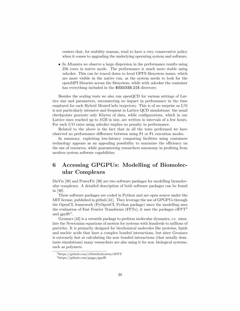
centers that, for stability reasons, tend to have a very conservative policywhen it comes to upgrading the underlying operating system and software.

• In Altamira we observe a large dispersion in the performance results using256 cores in native mode. The performance is much more stable usingudocker. This can be traced down to local GPFS filesystem issues, whichare more visible in the native run, as the system needs to look for theopenMPI libraries across the filesystem, while with udocker the containerhas everything included in the $UDOCKER DIR directory.

Besides the scaling tests we also run openQCD for various settings of Lat-tice size and parameters, encountering no impact in performance in the timeemployed for each Hybrid MonteCarlo trajectory. This is of no surprise as I/Ois not particularly intensive and frequent in Lattice QCD simulations: the usualcheckpoints generate only Kbytes of data, while configurations, which in ourLattice sizes reached up to 1GB in size, are written in intervals of a few hours.For such I/O rates using udocker implies no penalty in performance.

Related to the above is the fact that in all the tests performed we haveobserved no performance difference between using P1 or F1 execution modes.

In summary, exploiting low-latency computing facilities using containerstechnology appears as an appealing possibility to maximize the efficiency onthe use of resources, while guaranteeing researchers autonomy in profiting frommodern system software capabilities.

6 Accessing GPGPUs: Modelling of Biomolec-ular Complexes

DisVis [38] and PowerFit [39] are two software packages for modelling biomolec-ular complexes. A detailed description of both software packages can be foundin [40].

These software packages are coded in Python and are open source under theMIT license, published in github [41]. They leverage the use of GPGPUs throughthe OpenCL framework (PyOpenCL Python package) since the modelling usesthe evaluation of Fast Fourier Transforms (FFTs), it uses the packages clFFT3

and gpyfft4.Gromacs [42] is a versatile package to perform molecular dynamics, i.e. simu-

late the Newtonian equations of motion for systems with hundreds to millions ofparticles. It is primarily designed for biochemical molecules like proteins, lipidsand nucleic acids that have a complex bonded interactions, but since Gromacsis extremely fast at calculating the non–bonded interactions (that usually dom-inate simulations) many researchers are also using it for non–biological systems,such as polymers.

3https://github.com/clMathLibraries/clFFT4https://github.com/geggo/gpyfft

20

tag OS type of machinePhys-C7-QK5200 CentOS 7 PhysicalDock-C7-QK5200 CentOS 7 DockerDock-U16-QK5200 Ubuntu 16 DockerUDockP1-C7-QK5200 CentOS 7 udocker mode P1UDockP1-U16-QK5200 Ubuntu 16 udocker mode P1UDockF3-C7-QK5200 CentOS 7 udocker mode F3UDockF3-U16-QK5200 Ubuntu 16 udocker mode F3

Table 4: Execution environments for the DisVis and Gromacs applications.

6.1 Setup and deployment

The physical host used to benchmark udocker with the DisVis and Gromacsapplications using GPGPUs was made available by the Portuguese NationalDistributed Computing Infrastructure (INCD). It is hosted at the INCD maindatacenter in Lisbon and its characteristics are described in the Appendix.

The applications DisVis v2.0.0 and Gromacs 2016.3 were used. Docker im-ages were built from Dockerfiles for both applications and for two operating sys-tems: CentOS 7.3 (Python 2.7.5, gcc 4.8.5) and Ubuntu 16.04 (Python 2.7.12,gcc 5.4.0), the versions of the applications in the Docker images are the sameas in the physical host.

The applications in the Docker images were built with GPGPU supportand the NVIDIA software that matches the same version of the NVIDIA driverdeployed in the physical host system.

Those same images were then used to perform the benchmarks using bothDocker and udocker. In particular, udocker has several modes of execution(c.f. the user manual hosted at [10]), available through the setup --execmode

option. Two such options have been chosen for Gromacs execution, namely:P1 corresponding to PRoot with SECCOMP filtering and F3 corresponding toFakechroot with maximum isolation from the host system. For DisVis we onlyused the P1 execution mode.

Table 4 summarizes the different execution environments used in the bench-marks in terms of operating system and type of machine: physical (the host),Docker or udocker. The tags UDockP1 and UDockF3 correspond to the twochosen execution modes of udocker mentioned above.

6.2 Benchmark results

The DisVis use case was executed with input molecule PRE5-PUP2 complex.The application is executed with one GPU (the option -g selects the GPUexecution mode), using the following command:

$shell> disvis O14250.pdb \

Q9UT97.pdb \

21

Phys-C7 Dock-C7 Dock-U16 UDockP1-C7 UDockP1-U16Machine

0.90

0.92

0.94

0.96

0.98

1.00

1.02

1.04Ra

tio R

un ti

me

Disvis: case = PRE5-PUP2-complex Angle = 5.0 Voxelspacing = 1 GPU = QK5200

Ratio

Figure 5: Ratio between runtime values of Docker or udocker and the physicalhost of the DisVis use case. Lower values indicate better performance.

restraints.dat \

--angle 5.0 \

--voxelspacing 1 \

-g \

-d ${OUT_DIR}

The Gromacs gmx mdrun was executed with an input file of the amyloid betapeptide molecule. The application is executed with one GPU and 8 OpenMPthreads (per MPI rank), using the following command:

$shell> gmx mdrun -s md.tpr \

-ntomp 8 \

-gpu_id 0

For each case, 20 runs have been executed for statistical purposes. The runtime of each execution is recorded and a statistical analysis is done as follows:The outliers are detected and masked from the sample of 20 points, then theaverage and standard deviation are calculated for each case and environmentoption (physical host, Docker or udocker). The ratio between the average runtime of each docker or udocker environment with the average run time in thephysical host is plotted in Figures 5 and 6. Typical execution times for bothcases range between 20 and 30 minutes.

The first ratio (column) in each figure is 1 since the baseline is the physicalhost, the standard deviation of the ratio is calculated based on the statisticalformula for the ratio of two variables:

22

Phys-C7 Dock-C7 Dock-U16 UDockP1-C7 UDockP1-U16 UDockF3-C7 UDockF3-U16Machine

0.95

1.00

1.05

1.10

1.15

1.20

1.25Ra

tio R

un ti

me

Case = gromacs GPU = QK5200

Ratio

Figure 6: Ratio between runtime values of Docker or udocker and the physicalmachine of the Gromacs use case. Lower values indicate better performance.

∆R = ti/thost ×√

(∆ti/ti)2 + (∆thost/thost)2 (1)

Where: ti is the average runtime in a given environment, thost is the averageruntime in the physical host, ∆thost and ∆ti are the corresponded standarddeviations.

Figure 5 correspond to the benchmark of the DisVis use case. It can beseen that the execution of both Docker and udocker in CentOS 7.3 containersalthough 1 − 2% smaller than 1 is still compatible with this value. This showsthat executing the application in this type of virtualized environment has thesame performance as executing it in the physical host. On the other handexecuting the application in the Ubuntu 16.04 containers (both Docker andudocker cases) the execution time is around 5% better than in the physicalhost.

Figure 6 correspond to the benchmark of the Gromacs use case. It can beseen that the execution in CentOS 7.3 containers for Docker (second bar) andudocker with execution mode F3 (Fakechroot with maximum isolation from thehost system, sixth bar), are 3–5% worse than the execution in the physical hostalthough still compatible with one due to the statistical error. Also in the caseof execution in Ubuntu 16.04 containers (third and seventh bars) the ratios arecompatible with one, i.e. the containerized application execution has the sameperformance as in the physical host. In the case of executing the application inudocker containers with execution mode P1 (PRoot with SECCOMP filtering,forth and fifth bars), a penalty in performance of up to 22% is observed.

The difference in performance between udocker execution modes F3 and P1

23

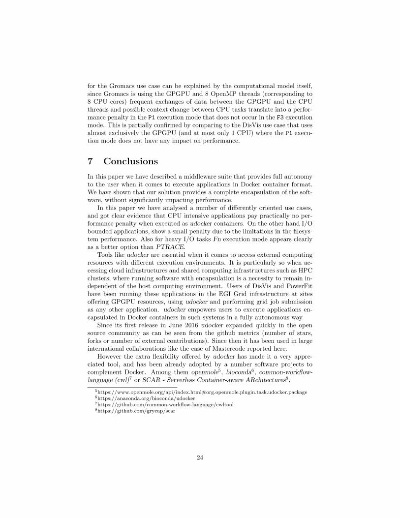
for the Gromacs use case can be explained by the computational model itself,since Gromacs is using the GPGPU and 8 OpenMP threads (corresponding to8 CPU cores) frequent exchanges of data between the GPGPU and the CPUthreads and possible context change between CPU tasks translate into a perfor-mance penalty in the P1 execution mode that does not occur in the F3 executionmode. This is partially confirmed by comparing to the DisVis use case that usesalmost exclusively the GPGPU (and at most only 1 CPU) where the P1 execu-tion mode does not have any impact on performance.

7 Conclusions

In this paper we have described a middleware suite that provides full autonomyto the user when it comes to execute applications in Docker container format.We have shown that our solution provides a complete encapsulation of the soft-ware, without significantly impacting performance.

In this paper we have analysed a number of differently oriented use cases,and got clear evidence that CPU intensive applications pay practically no per-formance penalty when executed as udocker containers. On the other hand I/Obounded applications, show a small penalty due to the limitations in the filesys-tem performance. Also for heavy I/O tasks Fn execution mode appears clearlyas a better option than PTRACE.

Tools like udocker are essential when it comes to access external computingresources with different execution environments. It is particularly so when ac-cessing cloud infrastructures and shared computing infrastructures such as HPCclusters, where running software with encapsulation is a necessity to remain in-dependent of the host computing environment. Users of DisVis and PowerFithave been running these applications in the EGI Grid infrastructure at sitesoffering GPGPU resources, using udocker and performing grid job submissionas any other application. udocker empowers users to execute applications en-capsulated in Docker containers in such systems in a fully autonomous way.

Since its first release in June 2016 udocker expanded quickly in the opensource community as can be seen from the github metrics (number of stars,forks or number of external contributions). Since then it has been used in largeinternational collaborations like the case of Mastercode reported here.

However the extra flexibility offered by udocker has made it a very appre-ciated tool, and has been already adopted by a number software projects tocomplement Docker. Among them openmole5, bioconda6, common-workflow-language (cwl)7 or SCAR - Serverless Container-aware ARchitectures8.

5https://www.openmole.org/api/index.html#org.openmole.plugin.task.udocker.package6https://anaconda.org/bioconda/udocker7https://github.com/common-workflow-language/cwltool8https://github.com/grycap/scar

24

Acknowledgements

This work has been performed in the framework of the H2020 project INDIGO-Datacloud (RIA 653549). The work of E.B. is supported by the CollaborativeResearch Center SFB676 of the DFG, “Particles, Strings and the early Uni-verse”. The proofs of concept presented have been performed at the FinisTerraeII machine provided by CESGA (funded by Xunta de Galicia and MINECO),at the Altamira machine (funded by the University of Cantabria and MINECO)and at the INCD-Infraestrutura Nacional de Computacao Distribuıda (fundedby FCT and P2020 under the project number 22153-01/SAICT/2016).

We are indebted to the managers of these infrastructures for their generoussupport and constant encouragement.

25

Appendix: Hardware and Software setup

The images of the containers used in this work are publicly available in theDocker hub, at the following urls:

• OpenQCD: https://hub.docker.com/r/iscampos/openqcd/

• DISVIS: https://hub.docker.com/r/indigodatacloudapps/disvis

• POWERFIT: https://hub.docker.com/r/indigodatacloudapps/powerfit

• MASTERCODE: https://hub.docker.com/r/indigodatacloud/docker-mastercode/

The proofs of concept presented have been carried out in the following infras-tructures, with the following Hardware/OS/Software setup:

• Finisterrae-II - CESGA, Santiago de Compostela

https://www.cesga.es/es/infraestructuras/computacion/FinisTerrae2

Hardware Setup:

– Processor type Intel(R) Xeon(R) CPU E5-2680 v3 @ 2.50GHz, withcache size 30MB

– Node configuration 2 CPUs Haswell 2680v3, (2x12 = 24 cores/node)and 128GB RAM/node

– Infiniband Network Mellanox Infiniband FDR@56Gbps

Software setup:

– Operating System CentOS 6

– Compilers GCC 6.3.0

– MPI libraries openmpi/2.0.2

• Altamira - IFCA-CSIC, Santander

https://grid.ifca.es/wiki/Supercomputing/Userguide

Hardware Setup:

– Processor type Intel(R) Xeon(R) CPU E5-2670 0 @ 2.60GHz, withcache size 20MB.

– Node configuration 2 CPUs E5-2670, (2x8 = 16 cores/node) and64GB RAM/node

– Infiniband Network Mellanox Infiniband FDR@56Gbps

Operating system and Software setup:

26

– Operating System CentOS 6

– Compilers GCC 5.3.0

– MPI libraries openMPI/1.8.3

• INCD, Lisbon

https://www.incd.pt

Hardware Setup:

– Processor type Intel(R) Xeon(R) CPU E5-2650L v3 @ 1.80GHz

– Node configuration 2 CPUs (2x12 = 24 cores/node x2 = 48 in HiperThread-ing mode) and 192GB RAM

– GPU model NVIDIA Quadro K5200

Operating system and Software setup:

– Operating System CentOS 7.3

– NVIDIA driver 375.26

– CUDA 8.0.44

– docker-engine 1.9.0

– udocker 1.0.3

References

[1] Linus Torvalds (2015). Linux Operating system.Can be retrieved from https://github.com/torvalds/linux/

[2] P. Menagehttps://www.kernel.org/doc/Documentation/cgroup-v1/cgroups.txt

[3] See https://en.wikipedia.org/wiki/Linux namespaces

[4] See eg. https://www.freebsd.org/doc/handbook/jails.html

[5] See https://linuxcontainers.org/lxc/ for a description of the project

[6] S. Hykes (Docker Inc)See software description and downloads in http://www.docker.com

[7] Description of the cloud-based Docker repository service can be found in:https://www.docker.com/products/docker-hub

[8] Kurtzer GM, Sochat V, Bauer MW (2017) Singularity: Scientificcontainers for mobility of compute. PLOS ONE 12(5): e0177459.https://doi.org/10.1371/journal.pone.0177459

27

[9] Jacobsen, Douglas M. and Richard Shane Canon. Contain This, UnleashingDocker for HPC. (2015).

[10] udocker can be downloaded from https://github.com/indigo-dc/udocker

[11] Quigley, David et al. Unionfs: User- and Community-Oriented Develop-ment of a Unification File System. (2006).

[12] See https://proot-me.github.io/

[13] See https://github.com/dex4er/fakechroot

[14] See https://nixos.org/patchelf.html

[15] See https://github.com/opencontainers/runc

[16] See https://www.opencontainers.org

[17] K. J. de Vries, PhD thesis Global Fits of Supersymmetric Models af-ter LHC Run 1 (2015), available on the Imperial College website:http://hdl.handle.net/10044/1/27056.

[18] L. Roszkowski, R. Ruiz de Austri, J. Silk and R. Trotta, Phys. Lett. B 671(2009) 10 doi:10.1016/j.physletb.2008.11.061 [arXiv:0707.0622 [astro-ph]].

[19] P. Bechtle, K. Desch and P. Wienemann, Comput. Phys. Commun. 174(2006) 47 doi:10.1016/j.cpc.2005.09.002 [hep-ph/0412012].

[20] L. Roszkowski, R. Ruiz de Austri, J. Silk and R. Trotta, Phys. Lett. B 671(2009) 10 doi:10.1016/j.physletb.2008.11.061 [arXiv:0707.0622 [astro-ph]].

[21] Behnel, S. and Bradshaw, R. and Citro, C. and Dalcin, L. and Seljebotn,D.S. and Smith, K., “Cython: The Best of Both Worlds”, Computing inScience & Engineering 13.2 (2011): 31-39, 10.1109/MCSE.2010.118.

[22] R. Brun and F. Rademakers, “ROOT: An object oriented data analysisframework,” Nucl. Instrum. Meth. A 389 (1997) 81. doi:10.1016/S0168-9002(97)00048-X

[23] Walt, S. V. D., Colbert, S. C., & Varoquaux, G. (2011), “The NumPy array:a structure for efficient numerical computation.”, Computing in Science &Engineering, 13(2), 22-30.

[24] Hunter, J. D. (2007), “Matplotlib: A 2D graphics environment”, Comput-ing In Science & Engineering, 9(3), 90-95.

[25] T. Hahn, Comput. Phys. Commun. 180 (2009) 1681doi:10.1016/j.cpc.2009.03.012

[26] F. Feroz, M. P. Hobson and M. Bridges, Mon. Not. Roy. Astron. Soc. 398(2009) 1601 doi:10.1111/j.1365-2966.2009.14548.x [arXiv:0809.3437 [astro-ph]].

28

[27] B. C. Allanach, Comput. Phys. Commun. 143 (2002) 305doi:10.1016/S0010-4655(01)00460-X [hep-ph/0104145].

[28] S. Heinemeyer et al., JHEP 0608 (2006) 052 [arXiv:hep-ph/0604147];S. Heinemeyer, W. Hollik, A. M. Weber and G. Weiglein, JHEP 0804(2008) 039 [arXiv:0710.2972 [hep-ph]].

[29] S. Heinemeyer, W. Hollik and G. Weiglein, Comput. Phys. Commun. 124(2000) 76 [arXiv:hep-ph/9812320]; S. Heinemeyer, W. Hollik and G. Wei-glein, Eur. Phys. J. C 9 (1999) 343 [arXiv:hep-ph/9812472]; G. Degrassi,S. Heinemeyer, W. Hollik, P. Slavich and G. Weiglein, Eur. Phys. J.C 28 (2003) 133 [arXiv:hep-ph/0212020]; M. Frank et al., JHEP 0702(2007) 047 [arXiv:hep-ph/0611326]; T. Hahn, S. Heinemeyer, W. Hollik,H. Rzehak and G. Weiglein, Comput. Phys. Commun. 180 (2009) 1426;T. Hahn, S. Heinemeyer, W. Hollik, H. Rzehak and G. Weiglein, Phys.Rev. Lett. 112 (2014) 14, 141801 [arXiv:1312.4937 [hep-ph]]; H. Bahl andW. Hollik, Eur. Phys. J. C 76 (2016) 499 [arXiv:1608.01880 [hep-ph]]. Seehttp://www.feynhiggs.de .

[30] P. Bechtle, O. Brein, S. Heinemeyer, G. Weiglein and K. E. Williams, Com-put. Phys. Commun. 181 (2010) 138 [arXiv:0811.4169 [hep-ph]], Comput.Phys. Commun. 182 (2011) 2605 [arXiv:1102.1898 [hep-ph]]; P. Bechtle etal., Eur. Phys. J. C 74 (2014) 3, 2693 [arXiv:1311.0055 [hep-ph]]; P. Bech-tle, S. Heinemeyer, O. Stal, T. Stefaniak and G. Weiglein, Eur. Phys. J. C75 (2015) no.9, 421 [arXiv:1507.06706 [hep-ph]].

[31] P. Bechtle, S. Heinemeyer, O. Stal, T. Stefaniak and G. Weiglein, Eur. Phys.J. C 74 (2014) 2, 2711 [arXiv:1305.1933 [hep-ph]]; JHEP 1411 (2014) 039[arXiv:1403.1582 [hep-ph]].

[32] G. Belanger, F. Boudjema, A. Pukhov and A. Semenov, Comput. Phys.Commun. 185 (2014) 960 [arXiv:1305.0237 [hep-ph]], and referencestherein.

[33] Information about this code is available from K. A. Olive: it containsimportant contributions from J. Evans, T. Falk, A. Ferstl, G. Ganis, F. Luo,A. Mustafayev, J. McDonald, F. Luo, K. A. Olive, P. Sandick, Y. Santoso,C. Savage, V. Spanos and M. Srednicki.

[34] M. Muhlleitner, A. Djouadi and Y. Mambrini, Comput. Phys. Commun.168 (2005) 46 [hep-ph/0311167].

[35] G. Isidori and P. Paradisi, Phys. Lett. B 639 (2006) 499 [arXiv:hep-ph/0605012]; G. Isidori, F. Mescia, P. Paradisi and D. Temes, Phys. Rev.D 75 (2007) 115019 [arXiv:hep-ph/0703035], and references therein.

[36] Martin Luscher,Code available at: http://luscher.web.cern.ch/luscher/openQCD

29

[37] Martin Luscher,Lectures given at the Summer School on Modern perspectives in latticeQCD, Les Houches, August 3-28 (2009)Downloadable at arxiv.org/abs/1002.4232

[38] G.C.P. Van Zundert, A.M.J.J. Bonvin, DisVis: quantifying and visualizingthe accessible interaction space of distancerestrained biomolecular com-plexes, Bioinformatics 31 (2015) 3222–3224

[39] G.C.P. Van Zundert, A.M.J.J. Bonvin, Fast and sensitive rigid-body fittinginto cryo-EM density maps with PowerFit, AIMS Biophys. 2 (2015) 73–87.

[40] G.C.P. van Zundert, et al., The DisVis and PowerFit Web Servers: Explo-rative and Integrative Modeling of Biomolecular Complexes, J. Mol. Biol.(2016), http://dx.doi.org/10.1016/j.jmb.2016.11.032

[41] DisVis: https://github.com/haddocking/disvisPowerFit: https://github.com/haddocking/powerfit

[42] Abraham, M. J., et al., GROMACS: High performance molecular simula-tions through multi-level parallelism from laptops to supercomputers, Soft-wareX 2015, 1–2, 19– 25 DOI: 10.1016/j.softx.2015.06.001

30