Identification and Modeling of the Airbrake of an

https://doi.org/10.1007/s10846-020-01204-1

Identification andModeling of the Airbrake of an ExperimentalUnmanned Aircraft

Peter Bauer1 · Lysandros Anastasopoulos2 · Franz-Michael Sendner3 ·Mirko Hornung2 · Balint Vanek1

Received: 19 October 2019 / Accepted: 15 April 2020© The Author(s) 2020

AbstractThis paper presents the modeling, system identification, simulation and flight testing of the airbrake of an unmannedexperimental aircraft in frame of the FLEXOP H2020 EU project. As the aircraft is equipped with a jet engine with slowresponse an airbrake is required to increase deceleration after speeding up the aircraft for flutter testing in order to remaininside the limited airspace granted by authorities for flight testing. The airbrake consists of a servo motor, an openingmechanism and the airbrake control surface itself. After briefly introducing the demonstrator aircraft, the airbrake design andthe experimental test benches the article gives in depth description of the modeling and system identification referencing alsoprevious work. System identification consists of the determination of the highly nonlinear (saturated and load dependent)servo actuator dynamics and the nonlinear aerodynamic and mechanical characteristics including stiffness and inertia effects.New contributions relative to the previous work are a unified servo angular velocity limit model considering opening againstthe load or closing with it, the detailed construction and evaluation of airbrake normal and drag force models consideringthe whole deflection and aircraft airspeed range, the presentation of a unified aerodynamic - mechanic nonlinearity modelgiving direct relation between airbrake angle, dynamic pressure and servo torque and the transfer function-based modeling ofstiffness and inertial effects in the mechanism. The identified servo dynamical model includes system delay, inner saturation,the aforementioned load dependent angular velocity limit model and a transfer function model. The servo model was verifiedbased-on test bench measurements considering the whole opening angle and dynamic load range of the airbrake. New,unpublished measurements with gradually increasing servo load as the servo moves are also considered to verify the model inmore realistic circumstances. Then the full airbrake model is constructed and tested in simulation to check realistic behavior.In the next step the airbrake model integrated into the nonlinear simulation model of the FLEXOP aircraft is tested by flyingsimulated test trajectories with the baseline controller of the aircraft in software-in-the-loop (SIL) Matlab simulation. First,the standalone airbrake simulation is compared to the SIL results to verify flawless integration of airbrake model into thenonlinear aircraft simulation. Then deceleration times with and without airbrake are compared underlining the usefulnessof the airbrake in the test mission. Finally, real flight data is used to verify and update the airbrake model and show theeffectiveness of the airbrake.

Keywords Aircraft airbrake · Dynamic test bench · System identification · Simulation · Flight test results

The research leading to these results is part of the FLEXOPproject. This project has received funding from the EuropeanUnions Horizon 2020 research and innovation program undergrant agreement No 636307. Part of this research has receivedfunding from the European Union’s Horizon 2020 researchand innovation programme under grant agreement No 815058(FLiPASED project).

� Peter [email protected]

1 Systems and Control Laboratory, Institute for ComputerScience and Control (SZTAKI), Kende utca 13-17, Budapest,H-1111, Hungary

1 Introduction

The FLEXOP EU H2020 research project [2] targeted todevelop an experimental aircraft (see Fig. 1) with inter-changeable wings (a rigid, a flexible and an aeroelastically

2 Department of Mechanical Engineering, Instituteof Aircraft Design, Technical University of Munich (TUM),Boltzmannstr. 15, Garching b., Munich, 85748, Germany

3 Research & Technology, FACC Operations GmbH,Breitenaich 52, Sankt Martin im Innkreis, A-4973, Austria

/ Published online: 6 June 2020

Journal of Intelligent & Robotic Systems (2020) 100:259–287

http://crossmark.crossref.org/dialog/?doi=10.1007/s10846-020-01204-1&domain=pdf

http://orcid.org/0000-0002-1925-2270

mailto: [email protected]

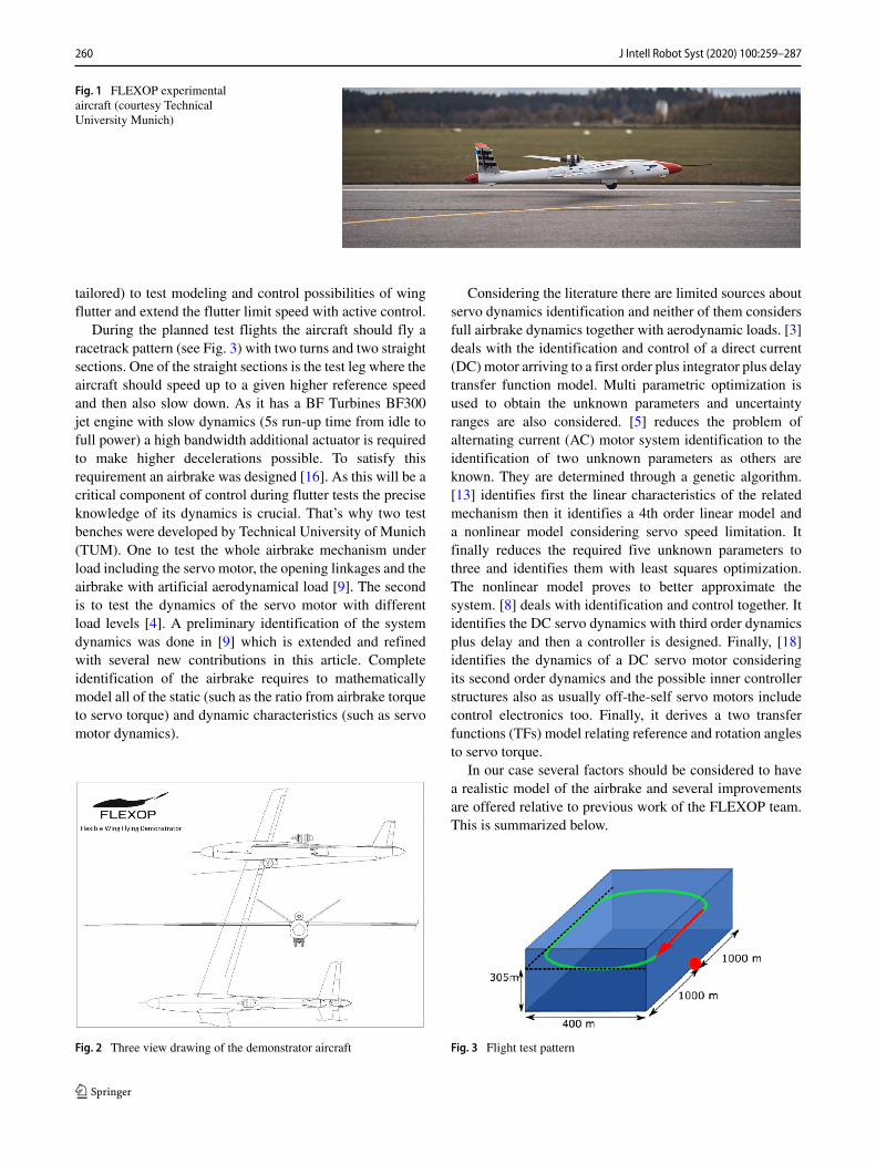
Fig. 1 FLEXOP experimentalaircraft (courtesy TechnicalUniversity Munich)

tailored) to test modeling and control possibilities of wingflutter and extend the flutter limit speed with active control.

During the planned test flights the aircraft should fly aracetrack pattern (see Fig. 3) with two turns and two straightsections. One of the straight sections is the test leg where theaircraft should speed up to a given higher reference speedand then also slow down. As it has a BF Turbines BF300jet engine with slow dynamics (5s run-up time from idle tofull power) a high bandwidth additional actuator is requiredto make higher decelerations possible. To satisfy thisrequirement an airbrake was designed [16]. As this will be acritical component of control during flutter tests the preciseknowledge of its dynamics is crucial. That’s why two testbenches were developed by Technical University of Munich(TUM). One to test the whole airbrake mechanism underload including the servo motor, the opening linkages and theairbrake with artificial aerodynamical load [9]. The secondis to test the dynamics of the servo motor with differentload levels [4]. A preliminary identification of the systemdynamics was done in [9] which is extended and refinedwith several new contributions in this article. Completeidentification of the airbrake requires to mathematicallymodel all of the static (such as the ratio from airbrake torqueto servo torque) and dynamic characteristics (such as servomotor dynamics).

Fig. 2 Three view drawing of the demonstrator aircraft

Considering the literature there are limited sources aboutservo dynamics identification and neither of them considersfull airbrake dynamics together with aerodynamic loads. [3]deals with the identification and control of a direct current(DC) motor arriving to a first order plus integrator plus delaytransfer function model. Multi parametric optimization isused to obtain the unknown parameters and uncertaintyranges are also considered. [5] reduces the problem ofalternating current (AC) motor system identification to theidentification of two unknown parameters as others areknown. They are determined through a genetic algorithm.[13] identifies first the linear characteristics of the relatedmechanism then it identifies a 4th order linear model anda nonlinear model considering servo speed limitation. Itfinally reduces the required five unknown parameters tothree and identifies them with least squares optimization.The nonlinear model proves to better approximate thesystem. [8] deals with identification and control together. Itidentifies the DC servo dynamics with third order dynamicsplus delay and then a controller is designed. Finally, [18]identifies the dynamics of a DC servo motor consideringits second order dynamics and the possible inner controllerstructures also as usually off-the-self servo motors includecontrol electronics too. Finally, it derives a two transferfunctions (TFs) model relating reference and rotation anglesto servo torque.

In our case several factors should be considered to havea realistic model of the airbrake and several improvementsare offered relative to previous work of the FLEXOP team.This is summarized below.

Fig. 3 Flight test pattern

260 J Intell Robot Syst (2020) 100:259–287

1. Identification of the servo dynamics itself is a challengeas the literature sources also show. First a servo testbench was developed and measurements with doubletseries servo angle references on different frequenciesand with different load torque levels were carried out(see [4] and [9]). In our case system identification iscomplicated by saturation in the inner servo controller(control saturation also considered in [13]) and loaddependent maximum angular velocities of the servowhich differ if servo travels against or with the load(similar load issue is considered in [18]). This issue ispartly covered in [9] but a simpler and unified modelis derived in the current work. Pulling out all thenonlinearities and system delay (also identified) finally,a transfer function model of the servo is identified usingthe output error method [11]. As the measurementsshow a load dependent steady-state servo angle changein the system output (missing I term in servo control) aseparate transfer function model was identified for thisand the need for this term verified based-on real flightbehavior. This is also a new contribution.

2. The nonlinear aerodynamics is covered by [9] onlyfor 60m/s maximum flight speed and only for thenormal force. Regarding that model the addition of thedrag coefficient and the drawing of the opening angle-airspeed-servo load characteristic is the contribution ofthis paper.

3. Regarding the nonlinearity in the opening mechanismdescribed in [9] (examined also in [13] for anothersystem) the contribution of the current paper is theconstruction of a unified aerodynamic plus mechanicnonlinear model to determine a direct relation betweenairbrake angle, dynamic pressure and servo torque. Theprecision of this model is also analysed.

4. A final challenge is the stiffness of the mechanism wellanalysed in [9]. Our contribution here is the transferfunction-based frequency domain analysis of systemdynamics considering stiffness and airbrake inertia.

The complete servo model was verified based onthe test bench measurements (adding new variable loadmeasurements to the previous work) and a full airbrakemodel was created after including servo motor model,opening mechanism and aerodynamic nonlinearity, stiffnessand load dependent steady-state servo angle change. Thismodel was first tested for realistic behaviour in Matlabsimulations then integrated into the nonlinear simulationmodel of the FLEXOP aircraft and tested with software-in-the-loop ‘flights’ of the test pattern with baseline trajectorytracking controller (see [14]) applying airbrake openingduring aircraft deceleration after the test leg. Finally, realflight measured position data of the airbrake is compared tothe simulation model (driven by in-flight logged dynamic

pressure and deflection command) output to verify theidentified model. The airbrake effect on aircraft decelerationwas also examined based-on the change in specific energyof the system.

The structure of the current paper is as follows. Section 2briefly introduces the test aircraft and the design of theairbrake then Section 2.1 summarizes the overall concept ofairbrake test and identifiaction. After that Section 3 givesbrief information about the test benches. Section 4 presentsthe identification of the nonlinear airbrake dynamics,Section 5 introduces the full airbrake model with SILsimulation results in Section 5.1 and real flight test resultsin Section 5.2. Finally, Section 6 concludes the paper.

2 Airbrake Conceptual Design

Before discussing airbrake conceptual design the FLEXOPdemonstrator aircraft and its operational circumstancesshould be briefly introduced to clarify the need andthe requirements related to the airbrake. The generalconfiguration of the FLEXOP demonstrator is of aconventional design asserting close similarity to state-of-the-art commercial aircraft. An illustrative three view ofthe actual demonstrator is depicted in Fig. 2 together withmain technical data in Table 1 (regarding the flutter speedsee [17]). The high aspect ratio wings feature a moderateleading edge sweep to account for the characteristic bend-twist-coupling of high-subsonic planform designs. The finalgoal with the demonstrator is to prove possibility of flyingbeyond flutter onset speed applying active control of thewing dynamics. To isolate wing aeroelastics from thrustinterferences and aerodynamic disturbances, an engineinstallation separated from the wings (on top of thefuselage) was chosen. Also a V-Tail for low-interferencedrag, as well as for minimum wetted area fuselage wasapplied. The required disturbance tolerance covers toleranceof moderate turbulence and deterministic wind disturbancesuntil 5-10m/s as the 65kg mass of the aircraft make it asmall one relative to the usual GA or larger aircraft. In futureflutter control tests as turbulence and wind free weather as

Table 1 FLEXOP demonstrator technical data

Wingspan 7m

Wing area 2.45m2

Aspect ratio 20

Leading edge sweep 20◦

Takeoff mass 65kg

Cruise speed 38m/s

Flutter onset speed 51m/s

Max engine thrust 300N

261J Intell Robot Syst (2020) 100:259–287

possible is required to remove additional disturbances of thestructural dynamics.

As the test airfield for the demonstrator is MunchenOberpfaffenhofen all operations should obey Germanairspace regulations. According to these regulations flighttesting within the visual line of sight of a human pilotis required. The flight altitude is limited to a maximumof 305m above ground level due to the procedures of theairfield operator. A maximum distance between pilot andvehicle in the order of 1000m was considered to providethe required visibility (considering the 7m wingspan of thedemonstrator) and so a flight test pattern as illustrated inFig. 3 is assumed. In the figure the position of the pilot ismarked with a red dot, with the resulting straight leg foraeroelastic (flutter) test phases marked by a red arrow [15].

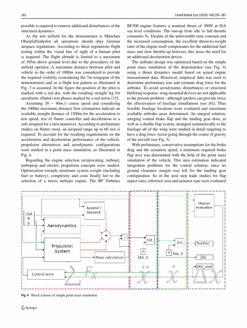
Assuming 38 − 40m/s cruise speed and consideringthe 1000m maximum distance first estimations indicate anavailable straight distance of 1500m for the acceleration totest speed, test of flutter controller and deceleration to asafe airspeed for a turn maneuver. According to preliminarystudies on flutter onset, an airspeed range up to 60 m/s isrequired. To account for the resulting requirements on theacceleration and deceleration performance of the vehicle,propulsion alternatives and aerodynamic configurationswere studied in a point mass simulation, as illustrated inFig. 4.

Regarding the engine selection reciprocating, turbojet,turboprop and electric propulsion concepts were studied.Optimization towards minimum system weight (includingfuel or battery), complexity and costs finally led to theselection of a micro turbojet engine. The BF Turbines

BF300 engine features a nominal thrust of 300N at ISAsea level conditions. The run-up from idle to full throttleconsumes 5s. Despite of the unfavorable time constant andthe increased consumption, the excellent thrust-to-weightratio of the engine itself compensates for the additional fuelmass and slow throttle-up however, this arose the need foran additional deceleration device.

The airbrake design was optimized based-on the simplepoint mass simulation of the demonstrator (see Fig. 4)using a thrust dynamics model based on actual enginemeasurement data. Historical, empirical data was used todetermine preliminary size and estimate drag force for theairbrake. To avoid aerodynamic disturbances or structuralbuffeting response, wing mounted devices are not applicableto the present problem - although spoilers can provide twicethe effectiveness of fuselage installations (see [6]). Thusfeasible fuselage locations were evaluated and maximumavailable airbrake areas determined. An integral solution,merging ventral brake flap and the landing gear door, aswell as a double flap system, arranged symmetrically to thefuselage aft of the wing were studied in detail targeting tohave a drag force vector going through the center of gravityof the aircraft (see Fig. 5).

With preliminary, conservative assumptions for the brakedrag and the actuation speed, a minimum required brakeflap area was determined with the help of the point masssimulation of the vehicle. This area estimation indicatedintegration problems for the ventral solution, since noground clearance margin was left for the landing gearconfiguration. So in the next step trade studies for flapaspect ratio, reference area and actuator type were evaluated

Fig. 4 Block scheme of simple point mass simulation


Fig. 5 Ventral and symmetricside-by-side arrangement of thebrake flaps (from left to right)

for the side-by-side flap configuration. A simple actuatormodel assuming either a linear or a rotary actuatorwas derived based on manufacturer specifications. Deadtime and actuator dynamics were neglected. A simpletransmission ratio rule was used for the preliminary models.The transmission concept is shown in Fig. 6.

Both linear and rotary models were integrated into thepoint mass vehicle simulation to evaluate the best fittingconcept. At maximum airspeed, the total deflection timeaccounted to 3.3 s for the linear actuator and below 0.5 s forthe rotary actuator. In consequence, only a rotary actuatorcould provide the required short deceleration distance asrendered previously (for details see [16]). So, finally theside-by-side flap configuration and a KST X30-12-150rotary servo actuator were selected as the main componentsof the airbrake system. After implementation of the wholesystem in a mock-up (see Fig. 8) and satisfactory testresults installation into the demonstrator fuselage was done.However, to study effects on system dynamics and to tuneon-board controllers a mathematical simulation model ofthe airbrake was required the construction and identificationof which is the main topic of this article as follows.

2.1 Airbrake System Identification Concept

The identification of the airbrake is a complex task as sev-eral parameters and characteristics should be determined.The final construction of the airbrake consists of the servomotor, the opening mechanism and the airbrake itself (seeFig. 37). Going from the inner part to the outer first, thedynamics of the servo motor was determined by build-ing a servo motor test bench (for details see Section 3.2)with a load motor which can be configured to apply dif-ferent torque loads (consant / varying) on the shaft of theservo. Different dynamic deflections of the servo with dif-ferent loads were done to cover the whole operational range(see Section 4.1 for the identification of servo dynamics).

After identification the servo model was verified based-ontest bench measurements. Second the aerodynamic char-acteristics of the airbrake were determined including thegenerated drag force which slows down the aircraft and theload torque on the airbrake shaft resulting from the aerody-namic load. As wind tunnel testing is time consuming andexpensive and there is exhaustive literature about such char-acteristics [6, 12] the aerodynamics was finally determinedbased-on published formulas (see Section 4.2). Finally, thestatic characteristics were determined such as the ratio ofthe mechanism from airbrake torque to servo torque and thestiffness of the whole mechanism as this can have a sig-nificant effect on the dynamics. The ratio was determinedbased-on geometrical measurements, however the stiffnessrequired to build a complete airbrake mock-up including theservo motor, the opening mechanism and the airbrake itselfwith the possibility to add different weights to simulate theaerodynamic loads (for details see Section 3.1). Measuringthe deformations with different loads gave the opportunityto determine the opening angle dependent stiffness of themechanism (see Section 4.2 for the static characteristics).An additional task was to determine the dynamic effect ofopening mechanism stiffness and airbrake flap inertia on theoverall dynamics. After constructing and identifying all ofthese model components and building the whole airbrakemodel the next task was to verify it in Software-in-the-loop(SIL) simulation and on real flight data. This is summarizedin Section 5.

3 Actuator Test Benches

To make determination of airbrake static and dynamiccharacteristics possible two test benches were built one isa full size mock-up which also serves to test the wholeairbrake opening mechanism together with the servo motorbefore installing it on the aircraft. The second is a separate

Fig. 6 Conceptual sketches oflinear and rotary actuation (fromleft to right)


Fig. 7 Side and isometric viewof the airbrake mock-up design(from left to right)

test bench for the servo motor applying an electric loadmotor to simulate airbrake loading on the servo axle.

3.1 Full Size AirbrakeMock-Up

A mass-loaded mock-up of the airbrake installation is usedto statically determine the full system stiffness over therange of deflection angles, as well as the static electricpower consumption. The mock-up consists of the actuallevers and rods, the airbrake flap, the servo actuator aswell as a mounting rig. The servo actuator is powered bya laboratory power supply, limited to 20A. The voltageis set to a constant value of 12V . The stiffness ofthe rig is designed such that the angular error inducedby the deflection of the assembly under maximum load

accumulates to 0.0023◦ giving minimal distortion in thedeflection measurement of the airbrake itself. A DigitalPitch Gauge (DPG), as well as a potentiometer is usedfor the determination of the deflection. As the maximumairspeed induced by the angular velocity of the airbrake flapis negligible relative to the 38-60 m/s speed of the aircraft nounsteady correction of the aerodynamic forces was requiredto be applied. So a simple mass carriage/swing was usedto solely apply a force normal to the airbrake. Within thequasi-linear load range up to 40◦, a mass of 12.658kg isused to simulate the aerodynamic load. For the range up to60◦, the mass ballast was adapted to match with the higheraerodynamic load (for details see [9]). The drawings of themock-up are shown in Fig. 7 while the photos can be seenin Fig. 8.

Fig. 8 Airbrake mock-up withclosed and fully opened airbrake(from left to right)


Fig. 9 Servo test bench withoutload (5: UAV actuator powersupply & command, 6: opticalencoder, the source is [4])

3.2 Servo Actuator Test Bench

In order to assist the identification of the airbrake servoactuator performance and allow for the derivation of a math-ematical model representing its operating characteristics, adynamometer test bench was developed [4]. It offers twomain testing modes: a force-free configuration (see Fig. 9)where actuator movement is monitored in the absence ofan external load and a torque-loaded configuration wherea counter load is applied in a controlled manner by a loadmachine (see Fig. 10). In the first mode the servo actuatoroutput shaft is connected to an angular position encoder thelatter possessing negligible friction and moment of inertia.In the second mode the servo actuator output shaft is con-nected to a load machine with a torque sensor placed insidethe load path between the two units. The next part focuseson the measurement campaign with the latter configuration(Fig. 10).

Linear systems are often represented by means of atransfer function or a state-space model and offer the

convenience, that classical model-based control algorithmscan be applied on them. However, in the present case,several nonlinearities are present in the servo actuatore.g.: the built-in angular position controller with currentand therefore angular velocity limitation and friction inthe airbrake actuator gearbox which dissipates kineticenergy nonlinearly. For this reason a simple linear modelrepresentation of the airbrake actuator dynamics shouldbe avoided. The implemented test scenarios are thereforetailored to the actual operation profile of the airbrake,which is designed to deflect against the airstream aroundthe fuselage. Combined with the propulsive engine, itis used to help aircraft deceleration during the missiontherefore dynamic deflections are expected in flight. Threetest campaigns are conducted with the loaded test bench(Table 4).

The results of the first two campaigns (Test campaignI & II) and a detailed description of the test setup arefound in [4] while results of Test campaign III are newlygenerated applying gradually increasing load as the servo

Fig. 10 Servo test bench with load (1: UAV actuator under test, 2: Torque sensor, 3: Beam coupling, 4: Load motor), the source is [4])


Fig. 11 Bode diagram of servo dynamics

moves and used only in this article. Evaluation of servoactuator performance in this realistic campaign is shown inTable 2 for different loads and the same deflection command(97.5◦). Later Test campaign III data is applied to verifythe realistic behavior of the servo model.

While the described test bench offered useful experi-mental data satisfactory to identify the basic mathematicalmodel of the airbrake servo certain limitations are to bepointed out and discussed:

1. Due to the hinge kinematics of the airbrake mechanism,radial forces are exerted against the actuator shaft,in addition to the torsional moment. However, at thetest bench the artificial load applied is solely thetorsional moment, the radial forces are thus neglected.Depending on the level of the latter, additional frictionon the actuator shaft bearing will arise. Successfulvalidation of the identified airbrake model in flight tests(see Section 5.2 and Fig. 55 for example) has shown thatthere is no significant such effect in the real system.

2. The load torque control algorithm of the load motorin the test bench is based on a feedforward path.Although actual torque is available in real time, additionof a torque feedback control path is avoided, due toinstabilities encountered. They are probably attributedto a slight delay in the load motor torque signal and the

high stiffness of the load path. As the identified servomodel describes the dynamics of the servo motor notthe load motor its not possible to examine this effectwith the identified model. Another issue is that at thebeginning of the actuator movement a peak is visibleat the torque profile (see Fig. 31) and also the currentprofile. This should be caused by the feedforwardcontrol experiencing a step change in the referencesignal and so commanding a very high input at the firsttime. This assumption is verified by the behavior forgradually increasing load torque command as there isno such peak in the measured torque as Fig. 34 shows.

3. Sampling is conducted with a frequency of 200 Hz.The maximum variation that can be accurately capturedis therefore less than 100 Hz. Current data howeversuggests that fluctuations of the actual signal mightbe more rapid. However, as the operating range of theairbrake will be at low frequency (bang-bang controlwith full opening or closing) the exact representationof very high frequency dynamics is not required. AsFig. 28 shows the servo motor is incapable to makefull range deflection even at 5Hz without load andlimited range deflections (Fig. 29) are also reduced byapplying load on the servo. So there is no possibility todrive the servo and so the airbrake with high frequencyreference inputs and so the limitation of the representedmeasured frequency range to 0-100Hz is more thenacceptable. This is also underlined by the Bode diagram(Fig. 11) of the identified servo motor dynamics (seriesconnection of Gref (z) reference signal dynamics fromEq. 1 considering the maximum AN(TL) = 6.1319gain if TL = 8Nm, Gsys(z) servo dynamics andthe integrator) also underlines this with 6.2rad/s =0.987Hz cut-off frequency and 8.85rad/s = 1.4Hz

bandwitdh. The maximum AN(TL) gain is largerthan the maximum AP (TL) and the maximum gaingives the maximum bandwidth that’s why this isconsidered.

System identification is discussed in the next sectionsincluding reproduction of measurement results of the servotest bench and SIL simulation of the whole nonlinearaircraft dynamics with flight test pattern tracking baselinecontrol without and with airbrake application during

Table 2 Evaluation of the airbrake actuator performance

Load Nm / 97.5◦ Steady angle [◦] Overshoot Ro [%] Rise time (10-90%) [s]

2 95.35 0.393 0.24

4 94.77 0.01 0.264

6 94.03 0.02 0.292

8 93.16 0.024 0.332


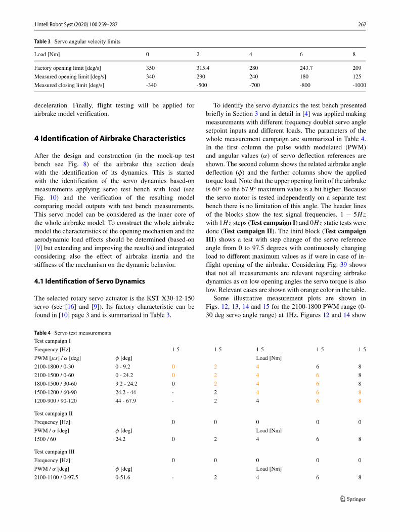
Table 3 Servo angular velocity limits

Load [Nm] 0 2 4 6 8

Factory opening limit [deg/s] 350 315.4 280 243.7 209

Measured opening limit [deg/s] 340 290 240 180 125

Measured closing limit [deg/s] -340 -500 -700 -800 -1000

deceleration. Finally, flight testing will be applied forairbrake model verification.

4 Identification of Airbrake Characteristics

After the design and construction (in the mock-up testbench see Fig. 8) of the airbrake this section dealswith the identification of its dynamics. This is startedwith the identification of the servo dynamics based-onmeasurements applying servo test bench with load (seeFig. 10) and the verification of the resulting modelcomparing model outputs with test bench measurements.This servo model can be considered as the inner core ofthe whole airbrake model. To construct the whole airbrakemodel the characteristics of the opening mechanism and theaerodynamic load effects should be determined (based-on[9] but extending and improving the results) and integratedconsidering also the effect of airbrake inertia and thestiffness of the mechanism on the dynamic behavior.

4.1 Identification of Servo Dynamics

The selected rotary servo actuator is the KST X30-12-150servo (see [16] and [9]). Its factory characteristic can befound in [10] page 3 and is summarized in Table 3.

To identify the servo dynamics the test bench presentedbriefly in Section 3 and in detail in [4] was applied makingmeasurements with different frequency doublet servo anglesetpoint inputs and different loads. The parameters of thewhole measurement campaign are summarized in Table 4.In the first column the pulse width modulated (PWM)and angular values (α) of servo deflection references areshown. The second column shows the related airbrake angledeflection (φ) and the further columns show the appliedtorque load. Note that the upper opening limit of the airbrakeis 60◦ so the 67.9◦ maximum value is a bit higher. Becausethe servo motor is tested independently on a separate testbench there is no limitation of this angle. The header linesof the blocks show the test signal frequencies. 1 − 5Hz

with 1Hz steps (Test campaign I) and 0Hz static tests weredone (Test campaign II). The third block (Test campaignIII) shows a test with step change of the servo referenceangle from 0 to 97.5 degrees with continuously changingload to different maximum values as if were in case of in-flight opening of the airbrake. Considering Fig. 39 showsthat not all measurements are relevant regarding airbrakedynamics as on low opening angles the servo torque is alsolow. Relevant cases are shown with orange color in the table.

Some illustrative measurement plots are shown inFigs. 12, 13, 14 and 15 for the 2100-1800 PWM range (0-30 deg servo angle range) at 1Hz. Figures 12 and 14 show

Table 4 Servo test measurements


60 60.5 61 61.5 62 62.5 63 63.5 64 64.5

Time [s]

-5

0

5

10

15

20

25

30

35P

osi

tion [

deg

.]

Position

Position setpoint

Fig. 12 1 Hz servo angle tracking at no load

that the measured servo angle overshoots the reference incase of no load. Note that in Fig. 14 the 8Nm load is appliedbetween about 64-66.7sec. The overshoot is possibly causedby the transient of the load motor. As the load motor modelis not identified this effect can not be studied in detail.Figure 14 shows that when a load is applied this overshoottransforms to undershoot causing negative deflection angleswhich are theoretically impossible. This can be causedby a missing I-term in servo control. In the servo modelidentification this change in the steady-state servo angle willbe considered by a transfer function from load torque toangle (see Subsubsection 4.1.3). If real flight test resultsverify this effect then this is built in to the servo model and isnot caused by the test bench. Evaluation of flight test resultsshows that the servo model including this effect well fits themeasured data so this is built in to the servo.

60 60.5 61 61.5 62 62.5 63 63.5 64 64.5

Time [s]

-500

-400

-300

-200

-100

0

100

200

300

400

500

An

gu

lar

vel

oci

ty [

deg

./s]

Angular velocity

Fig. 13 1 Hz angular velocity tracking at no load (Continuoushorizontal lines show the steady angular velocity values)

60 61 62 63 64 65 66 67 68 69

Time [s]

-5

0

5

10

15

20

25

30

35

Posi

tion [

deg

.]

Position

Position setpoint

Fig. 14 1 Hz servo angle tracking at maximum load (8Nm)

Figures 13 and 15 show that the possible angular velocityis limited inside the servo depending on the load. This is inagreement with the servo datasheet [10] as the first row ofTable 3 also shows. However, the real maximum openingvelocities against the load are lower then the values fromdatasheet. The approximate upper bounds are read from themeasurements and summarized in Table 3. In case if theservo moves with the load the angular velocities seem to bealmost unlimited, they have much larger absolute minimumvalues than maximums (except for the no-load case whenthe min/max angular velocities are the same, see Fig. 13).This case only approximate readings can be done againsummarized in Table 3. These are the approximate referencevalues where the servo seems to converge as in closing

60 61 62 63 64 65 66 67 68 69

Time [s]

-1000

-800

-600

-400

-200

0

200

400

Angula

r vel

oci

ty [

deg

./s]

Angular velocity

Fig. 15 1 Hz angular velocity tracking at maximum load (8Nm)(Continuous horizontal lines show the steady angular velocity valueswithout load, dashed lines show the with / against load values)


motion the angular velocity is in a transient at all the time(see Fig. 16).

The inner limitation of angular velocity by the actuatorelectronics made it impossible to identify simple transferfunction or state space system models from the referenceangle and torque to the output as in [18] for examplebecause there is characteristic difference between openingand closing speeds. That’s why nonlinearities were pulled-out and identified separately from the transfer functionmodels of the servo. Examining the measured data in detailshows that there can be an inner reference angular velocityvalue depending on the load and the angle tracking errorof the servo. The servo tracks this inner angular velocityreference (see Fig. 15 for example where the maximumangular velocity is almost constant during opening of theairbrake) with a given dynamics. So firstly this innerlimitation of the angular velocity reference and its trackingerror related dynamics is studied and identified in the nextpart.

4.1.1 Transfer Function Identification Between TrackingError and Angular Velocity Reference

At first, plotting together the angle tracking error andthe angular velocity (for the 1800 to 1500 PWM (30deg

to 60deg) 1Hz, 0Nm case in Fig. 17) shows that theangular velocity follows a square reference signal while thetracking error continuously changes. This means that thetracking error should be saturated to get a limited innerangular velocity reference from it. Note that consideringFigs. 12 and 14 there is a delay, an offset and a scaleerror between the reference servo angle and the real one.As possible negative angular values are present in the

Fig. 16 1Hz angular velocity tracking at maximum load (8Nm).Dashed lines show the with / against load values. Dotted line shows theexponential type convergence of the angular velocity to the selectedminimum value

62 62.05 62.1 62.15 62.2 62.25 62.3

Time [s]

0

5

10

15

20

25

Tracking error [deg]

Angular velocity [rad/s]

Fig. 17 Tracking error and angular velocity

measurement setup the 30deg to 60deg range was selectedfor identification to avoid them. All of the errors (delay,offset, scale error) were corrected before calculating thetracking error. The delay from the angle reference to theangular velocity was estimated to be 4 time steps (thesampling time is Δt = 0.005s) that’s why considering theabout one step delay of the discrete time form of transferfunctions in Eq. 1 3 steps delay was applied to the referencesignal. The offset and scale error are only considered inthe pre-scaling of data for system identification, they arenot considered in the final model as they are caused bymeasurement errors in the test bench.

Studying several cases and considering 3-4 steps delayfrom the start of saturated tracking error decrease to thestart of real angular velocity decrease has shown that thesaturation limit of the tracking error should be about 5.8◦ =0.10123rad .

An almost square reference can be easily generated by asimple transfer function from normalized saturated trackingerror to angular velocity reference in the form: G(s) =

AT s+1 however, for a positive tracking error the velocityreference limit should be different than for a negative andthis difference should depend on the load torque (TL) of theservo. The positive-negative difference can advantageouslybe described by the following system structure:

αref (s) = −AP (TL)

T s + 1· Δaα(s) + AN(TL)

T s + 1· Δα(s) (1)

where AP (TL), AN(TL) are load torque (TL) dependentscalar coefficients, T = 0.003s is the time constantdetermined by trial and error to give a realistic referenceconsidering the system answer (see Fig. 18), Δα = αref −α

and Δaα = |αref − α|. Compared to [9] this model unifiesthe decision about the opening or closing and the upper andlower angular velocity limitations. In the referenced workseparate upper and lower limiting curves were determined,the lower only valid until 2Hz, here the curves are unifiedand valid on the whole measured frequency range (1-5Hz).This improvement is achieved through the better estimation


61.1 61.15 61.2 61.25 61.3 61.35 61.4 61.45Time [s]

0

1

2

3

4

5

6

Angula

r vel

oci

ty [

rad/s

]

Measured velocity

Tracking error [rad!]

Estimated velocity reference

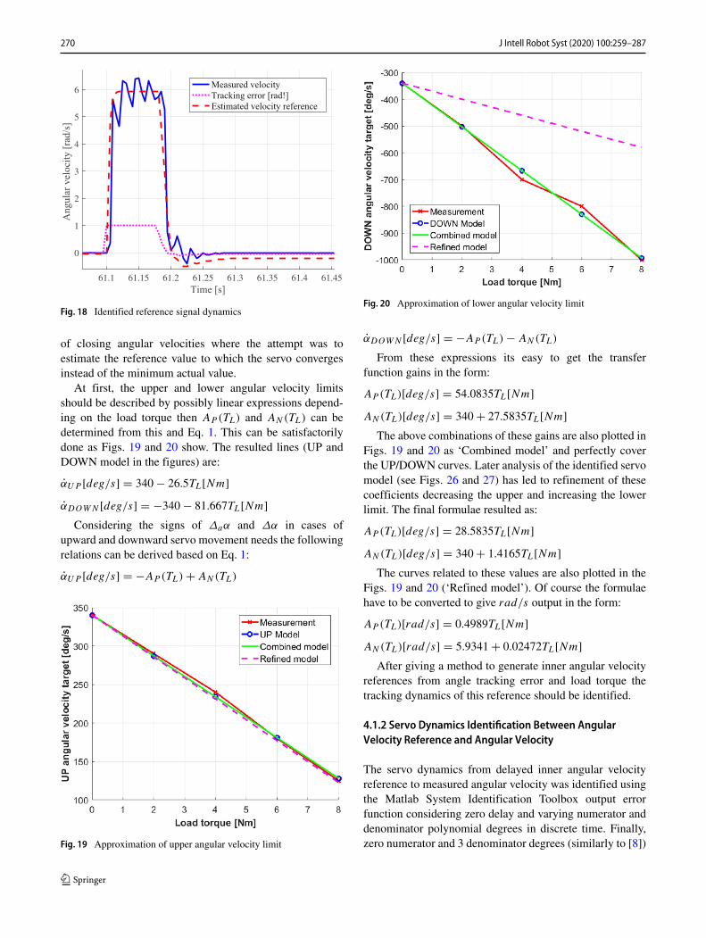
Fig. 18 Identified reference signal dynamics

of closing angular velocities where the attempt was toestimate the reference value to which the servo convergesinstead of the minimum actual value.

At first, the upper and lower angular velocity limitsshould be described by possibly linear expressions depend-ing on the load torque then AP (TL) and AN(TL) can bedetermined from this and Eq. 1. This can be satisfactorilydone as Figs. 19 and 20 show. The resulted lines (UP andDOWN model in the figures) are:

αUP [deg/s] = 340 − 26.5TL[Nm]αDOWN [deg/s] = −340 − 81.667TL[Nm]

Considering the signs of Δaα and Δα in cases ofupward and downward servo movement needs the followingrelations can be derived based on Eq. 1:

αUP [deg/s] = −AP (TL) + AN(TL)

Fig. 19 Approximation of upper angular velocity limit

Fig. 20 Approximation of lower angular velocity limit

αDOWN [deg/s] = −AP (TL) − AN(TL)

From these expressions its easy to get the transferfunction gains in the form:

AP (TL)[deg/s] = 54.0835TL[Nm]AN(TL)[deg/s] = 340 + 27.5835TL[Nm]

The above combinations of these gains are also plotted inFigs. 19 and 20 as ‘Combined model’ and perfectly coverthe UP/DOWN curves. Later analysis of the identified servomodel (see Figs. 26 and 27) has led to refinement of thesecoefficients decreasing the upper and increasing the lowerlimit. The final formulae resulted as:

AP (TL)[deg/s] = 28.5835TL[Nm]AN(TL)[deg/s] = 340 + 1.4165TL[Nm]

The curves related to these values are also plotted in theFigs. 19 and 20 (‘Refined model’). Of course the formulaehave to be converted to give rad/s output in the form:

AP (TL)[rad/s] = 0.4989TL[Nm]AN(TL)[rad/s] = 5.9341 + 0.02472TL[Nm]

After giving a method to generate inner angular velocityreferences from angle tracking error and load torque thetracking dynamics of this reference should be identified.

4.1.2 Servo Dynamics Identification Between AngularVelocity Reference and Angular Velocity

The servo dynamics from delayed inner angular velocityreference to measured angular velocity was identified usingthe Matlab System Identification Toolbox output errorfunction considering zero delay and varying numerator anddenominator polynomial degrees in discrete time. Finally,zero numerator and 3 denominator degrees (similarly to [8])


Fig. 21 Identified servo system dynamics

gave the best results as shown in Fig. 21 with 82.86% fit.This transfer function (Gsys(z)) has no zeros and poles:

0.4882 − 0.2515 ± 0.6483i

These discrete time poles are stable and oscillatory as themeasured system output is also oscillatory. The parametersof the transfer function are shown in the Appendix. Theslight offset error in the figure is the result of non-perfectoffset removal from reference - output signal pair (seeFig. 18 where the estimated velocity reference is onlyapproximately zero). Integrating the real angular velocity ofthe servo model gives servo deflection angle so this way theidentification of the servo dynamics is ready. However, aload dependent angular position offset was detected in thetest bench measurements (see Fig. 14) which should be alsoidentified. This is done in the next part.

-0.06

-0.04

-0.02

0

0.02Angle [rad]

0 0.5 1 1.5 2 2.5

0

2

4

6

8Load torque [Nm]

Input-Output Data

Time (seconds)

Am

plitu

de

Fig. 22 Effect of load application on servo angle

4.1.3 Load Dependent Servo Angle Offset Dynamics

Examining the measured data shows that application of theload moves the system steady-state servo angle with somevalue. This can be caused by a missing I-term in servocontrol electronics. Identification of the load torque (TL)output angle (α) offset dynamics can be done consideringload application in the fix 1500 PWM measurement cases.The delay between load and angle was estimated as 4 stepsand then a transfer function (GTL

(z)) with zero numeratorand one denominator degree was identified with 96.98% fit(parameters published in Appendix). The load change andangle change are shown in Fig. 22 and the transient of theidentified transfer function is shown in Fig. 23.

After identifying the reference and system dynamics aMatlab Simulink simulation for the servo model itself wasconstructed and the identified model verified driven by testbench data with load application. The block scheme of theSimulink model is shown in Fig. 24.

The block delay represents the 3 steps time delay ofthe reference. SAT and NORM represent saturation ofthe error signal to ±0.10123rad and normalization with

10.10123 = 9.8786 respectively. Gref (z) represents thediscrete time equivalent of the identified inner angularvelocity reference model (1)Gsys(z) is the identified systemmodel from angular velocity reference to angular velocityand GTL

(z) is the identified system model from load toangle including also the 4 steps time delay.

4.1.4 Servo Model Verification Based-on Measured TestBench Data

After the identification and Simulink model constructionthe dynamic model of the servo motor was verified based-on measured data from the servo test bench. As a first

Fig. 23 Transient of identified load to angle system model


Fig. 24 Simulink model of theservo

verification simulation results of the 2100 to 1800 PWM,1Hz, 0Nm and 4Nm measurement cases are shown inFigs. 25 and 26. 4Nm is the maximum realistic load inthis deflection range that’s why it was considered in modelverification instead of the 8Nm maximum load. Resultsof a simulation with the original lower angular velocityreference bounds with 4Nm load are also shown in Fig. 27.The first two figures show that the final system modelacceptably models the servo dynamics both without andwith load. In the third figure it can be seen that the originallower angular velocity bounds gave very large overshoot incase of downward moving servo that’s why the limits wereincreased (decreased in absolute value) and the expressionsfor AP (TL) and AN(TL) were modified.

As Fig. 24 shows the required inputs of the servo modelare reference deflection and load torque. The referencedeflection is given for all test bench measurement (seeFig. 26 for example) and the real load torque of the servois saved (see for example Fig. 31) so both can be given assimulation model input.

At first, the identified model was checked consideringa measurement from Test campaign I with full rangedeflection 0−120◦ at 5Hz square wave excitation with 8Nm

load application through some time. This is the most criticaltest case with the highest frequency and load. As Fig. 28

0 0.5 1 1.5 2 2.5 3 3.5 4 4.5Time [s]

-5

0

5

10

15

20

25

30

35

Angle

[deg

]

Angle dynamics

MeasuredSimulated

Fig. 25 Servo model with 0 to 30 degs reference zero load

shows this range with this frequency is too challengingfor the servo controller and it can not follow the referencesignal even with zero load. Comparison with data from theidentified model shows that there is a drift in the test benchbehavior which is not considered in identification.

Checking the model for test bench measurements witha tractable range (30 − 60◦) again from Test campaign Iin Fig. 29 shows that in normal mode there is neither driftin test bench output nor in identified model. Figure 29 alsoshows that the identified model well follows the behavior ofthe real servo considering the angular deflections. Figure 30shows the measured and simulated angular velocities andFig. 31 shows the reference and the measured torque of thetest bench for completeness.

The simulated angular velocities are close to the real onesexcept for the transient periods but the overall performanceis acceptable. So finally, the largest difference betweenmodel and measurements is the downward overshoot of theangle and the different behavior in the transients (whentorque is applied and removed). However, in these testbench measurements the maximum load torque was appliedimmediately which is not realistic considering the openingof the airbrake, there the maximum load torque appears onlyon maximum deflection and it increases gradually as the

0 1 2 3 4 5 6 7 8 9Time [s]

-5

0

5

10

15

20

25

30

35

An

gle

[d

eg]

Angle dynamics

MeasuredSimulated

Fig. 26 Servo model with 0 to 30 degs reference 4Nm load tightangular velocity limit


0 1 2 3 4 5 6 7 8 9Time [s]

-10

-5

0

5

10

15

20

25

30

35

An

gle

[d

eg]

Angle dynamics

MeasuredSimulated

Fig. 27 Servo model with 0 to 30 degs reference 4Nm load looseangular velocity limit

airbrake is opened. So if the model works well for graduallyincreasing realistic load torque then the different transientsin unrealistic circumstances do not cause a problem.

To verify the servo model with more realistic conditionstest bench measurements with gradually increasing (follow-ing the increase in opening angle) load torque from Testcampaign III are considered. Figures 32, 33 and 34 showthe results for the maximum load case when servo deflec-tion to 97.5◦ is followed by a load increase to 8Nm. Thefigures show that both the simulated angular velocity andangle follow well the measurements so the description ofthe real dynamics is satisfactory. The only difference is alarge angular velocity glitch in the measurements when the

Fig. 28 Measured and simulated servo angle dynamics in full range(0 − 120◦) at 5Hz and 8Nm square load

Fig. 29 Measured and simulated servo angle dynamics in limitedrange (30 − 60◦) at 5Hz and 8Nm square load

load is suddenly removed (see Fig. 34). Carefully examin-ing Fig. 32 shows that the identified model well follows thesmall angle change in this case (at about 12.5s) and so thelack of the glitch does not cause any discrepancy and so theidentified model’s behavior is acceptable.

After the verification of the servo model the staticcharacteristics of the opening mechanism and the airbrakeaerodynamic effects are examined and described in the nextsubsection together with the possible dynamic effects ofopening mechanism stiffness and airbrake inertia.

Fig. 30 Measured and simulated servo angular velocity dynamics inlimited range (30 − 60◦) at 5Hz and 8Nm square load


Fig. 31 Referenced and measured servo load torque (8Nm squareload) in limited range (30 − 60◦) 5Hz experiment

4.2 Determination of Static Characteristics

The most important static characteristic of the airbrake is theaerodynamics. Considering the dynamic pressure pdyn =ρ2V 2 known (here ρ is air density and V is airspeed) theaerodynamics can be described by the drag force cD andnormal force cN coefficients depending on the openingangle φ of the airbrake. The normal force coefficients arepublished in [9] while the drag force coefficients are firstpublished here in Table 5.

Regarding the drag the calculations were done consid-ering a flat plate with a given opening angle based on[12]. Plotting the data together (see Fig. 35) it seems to be

Fig. 32 Measured and simulated servo angle dynamics with graduallyincreasing load

Fig. 33 Measured and simulated servo anglular velocity dynamicswith gradually increasing load

Fig. 34 Gradually increasing load in servo test bench

Table 5 Aerodynamic data

φ[◦] cN a[mm] c′N cD

0 0 106.058 0 0

10 0.3 118.985 0.3366 0.18

20 0.65 131.912 0.8085 0.3

30 0.9 144.839 1.2291 0.5

40 1.21 157.766 1.8 0.8

50 1.1 170.693 1.7704 0.75

60 1.05 183.62 1.8179 0.9


Fig. 35 Line fit to airbrake angle - drag coefficient data

that the value at 40◦ is an outlier as it is out of the oth-erwise linear trend and so it is neglected when fitting aline to the data. A constrained line fit going through the(0◦, 0) point was done considering only opening angles[0◦ 10◦ 20◦ 30◦ 60◦] to provide a more balanced fitwith two points below and two above the resulting line(see Fig. 35). Considering also the 50◦ point moved the fitdown almost neglecting the upper points. On the contraryconsidering only the 0◦ to 30◦ range gave a line too upalmost neglecting the lower points as the figure shows. Theresulting polynomial cD(φ) can be found in the Appendix.

Regarding the normal force coefficient its applicationpoint also changes with the opening angle. This ischaracterized by the a(φ) arm length in Table 5. As thefinal goal is to get an airbrake model as compact as possibleits worth to unite the normal force coefficient and the armlength as

c′N(φ) = cN(φ)

a(φ)

aref

where aref = 106.058mm is the assumed fixed armlength. Considering the normalized c′

N(φ) coefficient twosections of the curve can be distinguished and so a parabolaand a line were fitted to the data as shown in Fig. 36.The formulae are presented in the Appendix. Based onc′N(φ) the normalized normal force can be calculated as

F ′N = c′

N(φ)pdynSref where Sref = 0.032675282m2 is theairbrake reference area (on one side).

The required servo torque to move the airbrake canbe calculated considering the geometry of the opening

Fig. 36 Curve fit to airbrake angle normal force coefficient data(continuous line: original data, dashed line: fitted curves)

mechanism in between shown in Fig. 37. In the figure thearm lengths are:

aref = 106.058mm

b = 68.417mm

c = 29.829mm

d = 112.698mm

e = 42.932mm

There is a nonlinear relation between the anglesβ, γ, δ, φ summarized in tabular form in Table 6. Note thatfor small β angles δ can be negative as shown in Fig. 37 andfor large β angles γ becomes negative (it is shown in thepositive range in the figure).

The servo torque for a given airbrake opening angle φ,airspeed V and air density ρ can be determined as:

T (φ) = e

1000

cos(δ(φ))

cos(γ (φ))

aref

bpdynSref · c′

N(φ)

= sa(φ)c′N(φ)pdyn (2)

In the second part of the equation all the geometricparameters are summarized in a virtual servo arm lengthsa(φ). The curves for c′

N(φ) are determined before so a

curve for the sa(φ) = e1000

cos(δ(φ))cos(γ (φ))

aref

bSref virtual servo

arm is required. Substituting the known fix parameters theonly angle dependent part remains cos(δ(φ))

cos(γ (φ)):

sa(φ)= 42.932

1000

106.058

68.4170.032675282

cos(δ(φ))

cos(γ (φ))=2.1744·10−3 cos(δ(φ))

cos(γ (φ))

The tabular data and the fitted 5th degree curve are shownin Fig. 38. The curve parameters are given in the Appendix.

After fitting polynomial models to the normal forcecoefficient and the virtual servo arm it is advisable to check


Fig. 37 The opening mechanism of the airbrake (β servo arm angle, φ airbrake opening angle

the precision of fitting. The largest servo torque will berequired on sea level so servo torque values are calculatedon sea level for airspeed from 10m/s to 60m/s and forall possible φ opening angles from Table 5. Calculationswere done both from the mechanism and tabular data andfrom the fitted curves. Figure 39 shows that the approximate(dashed) curves are close to the real ones at every pointwhile the absolute difference increases with airspeed. Therelative errors of the fits (percentage) are shown in Fig. 40.These percentages are independent from the air density andairspeed. The figure shows that the maximum error is about6% at φ = 10◦ and then the errors are decreasing. Therelative error can not be calculated for zero angle with zerotorque that’s why it is not plotted. Extrapolating the othervalues the relative error around zero angle can be about8 − 10%.

After fitting curves to the aerodynamic coefficients andmoment arm fast conversion formulae from servo angleα to airbrake angle φ and vice versa are required. Theservo angle α is different form the servo arm angle β. Itis defined to be zero at the minimum servo arm angle:

α = β − 18.612◦. Regarding the curve fits α − φ resultedas a 3rd degree polynomial going through zero while φ − α

as a 4th degree polynomial again going through zero. Thepolynomials are summarized in the Appendix while the fitqualities can be checked in Fig. 41 (they are superior).

Finally, the stiffness characteristics of the airbrakemechanism should be identified to increase precisionof deflection model considering the flexibility of themechanism. Theoretical airbrake deflection angle fromcommanded actuator position and transmission of the rigidkinematic chain and measured deflection angle from theairbrake mock-up (see Fig. 8) were compared for a givenset of measurement points. From the angle deviation, thesystem stiffness was derived (for details see [9]). The goalof this work was to extend the covered range by the stiffnessformula as only the φ opening range 20 − 60◦ was coveredby the model in [9]. Finally, the stiffness data was convertedfrom degrees φ angle input and output to radians and acurve fit was done on the data resulting in a third degreepolynomial (kφ) which is presented in the Appendix. Theplot of the stiffness against the opening angle can be seen in

Table 6 Angles of the mechanism

φ[◦] β[◦] γ [◦] δ[◦]

0 18.612 70.374 -22.247

10 50.3072 49.8725 -1.0533

20 71.5579 33.1459 13.4708

30 88.2593 17.1578 24.1841

40 102.4986 0.9717 32.2373

50 115.6444 -16.1956 38.2158

60 129.1891 -35.7065 42.2497


Fig. 38 Curve fit to airbrake angle virtual servo arm data (continuousline: original data, dashed line: fitted curve)

Fig. 42. The fitted formula can cover the whole angle range0 − 60◦ with reasonable non-negative values. As openingmechanism flexibility is present in the system its effects onthe dynamic behavior should be examined. This is the topicof the next part.

4.2.1 Effects of Airbrake Inertia and Mechanism Stiffness

The inertial moment of the flap was estimated by modellingthe flap as a rectangular prism with an external axis ofrotation in distance c = 51.5mm, as illustrated in Fig. 43.The length l = 218mm is assumed corresponding to theedge length of the actual flap, the width b according to

Fig. 39 Servo torque from mechanism (color continuous) and fromapproximation (magenta dashed). Lowest curve for 10 m/s whilehighest for 60 m/s airspeed

Fig. 40 Servo torque approximation errors

the mean width of the flap and the thickness d = 4mm

according to the actual sandwich core thickness of thestructure. An isotropic density distribution is assumed. Tocompensate for the external axis of rotation, the parallel-axes theorem is used. The inertial moment can be estimatedby using the following equation (see [7]):

I = m

(l2

12+ d2

12

)+ m

(l2

4+ c2

)(3)

With the second term being the compensation fromparallel axes theorem and using the measured mass m =0.115kg of the actual flap. As the formula shows the width(b) is not required to estimate the moment of inertia withregard to the given axis. Due to the slight trapezoidalplanform of the flap, the actual center of gravity is closer to

Fig. 41 Servo angle - airbrake angle curves


Fig. 42 Change of mechanical stiffness with opening angle

the axis of rotation. In consequence, the inertia is estimateda bit conservatively.

Figure 44 shows the simple dynamical model of theservo-airbrake setup considering the stiffness kφ of themechanism as a torsional spring. α is the servo arm angle(β) shifted to be zero at minimum deflection as α = β −18.612◦ while φ is the deflection angle of the airbrakeitself. For the relation between β and φ through the airbrakedeflection mechanism see Fig. 37. To simplify the modela one-to-one mapping between α and φ is assumed asany static gain between them would not modify dynamicbehavior. The servo torque T equals the elastic force in themechanism at every time as: T = kφ(α − φ).

The dynamic equation of the airbrake considering itsmass moment of inertia I = 2.127 · 10−3kgm2 the torqueof the aerial forces on the airbrake TL and the fact that it isdriven through the flexible mechanism results as:

I φ = kφ(α − φ) − TL

Note that here the airbrake load torque is transformedto the servo shaft (TL) and the stiffness of the mechanismis considered as a simple torsional spring between.Reorganizing the above expression and making Laplacetransform of each side results in two transfer functions, one

Fig. 43 Simple model of airbrake flap for inertia calculation

Fig. 44 Simple dynamic model with stiffness and inertia

from servo angle α to airbrake deflection φ: Gα(s) and onefrom aerial load TL to airbrake deflection φ: GL(s)

I φ + kφφ = kφα − TL (4a)

φ(s) = kφ

Is2 + kφ

α(s) + −1

Is2 + kφ

TL(s) (4b)

Gα(s) = kφ

Is2 + kφ

(4c)

GL(s) = −1

Is2 + kφ

(4d)

(4e)

So finally, one gets a two input (α servo angle andTL torque of aerial forces) one output (φ airbrake angle)system. Note that the kφ term depends on the actual angleof the airbrake (see Fig. 42) and so these transfer functionsshould be examined for different airbrake angle values.Bode plots were plotted for angle values 0 : 5◦ : 60◦covering the whole range and shown in Figs. 45 and 46.

Fig. 45 Bode plots for servo angle α input


Fig. 46 Bode plots for airbrake load TL input

They show that both term can be well approximatedwith a constant gain on a wide frequency range. They giveundamped oscillations only on high frequencies (well above70 rad/s=11Hz) on which the airbrake will not be operatedas its bandwidth is about 1.4Hz shown by Fig. 11. Anotherfact to be considered is that the mechanism should alsohave damping which is unknown but surely present and socould damp the oscillations to a favorable level even on highfrequencies. If flight testing does not show oscillations evenwith high frequency excitation then a static model includingonly the effect of stiffness can be used.

Considering low frequency approximations of the trans-fer functions one gets:

φ(s) = 1 · α(s) + −1

kφ

TL(s) (5)

Fig. 47 Simulink model of the whole airbrake

Taking the inverse Laplace transform and reorganizingthe terms gives:

TL = kφ(α − φ) = kφΔφ (6)

Where Δφ is the angular deformation and can be obtainedas Δφ = α − φ = TL

kφ. In the airbrake simulation the servo

deflection α and the momentarily load TL on the servo areknown and so kφ and φ can be obtained as shown in thestructure in Fig. 47.

5 Full Airbrake SimulationModel and TestResults

After identifying the model components the whole systemwith servo model, mechanism and aerodynamic effectswas constructed and simulated in Matlab Simulink. Theblock scheme of the whole simulation structure is shownin Fig. 47. Here, Servo is the servo simulation model fromFig. 24, pdyn calculates the dynamic pressure from ρ airdensity and V airspeed, α(φ) and φ(α) are the polynomialstransforming airbrake angle to servo angle and vice versa.kφ is the angle dependent stiffness coefficient, the loadtorque TL is divided by it to get the angle change (Δφ)of the airbrake as derived at the end of Section 4.2. To bea bit more realistic the whole angle change is subtractedfrom the airbrake position used to calculate air drag andnormal force, but only half of it is subtracted to calculate thevirtual servo arm sa(φ) assuming non-uniform deformationinside the mechanism. SAT represents the saturation of theairbrake angle output between 0rad and 1.0472rad (0 −60◦). The blocks with three × represent the multiplicationof all inputs. D is the air drag force as the useful output ofthe system contributing to the deceleration of the aircraft.


After the construction the model was tested with stepairbrake angle reference changes, airspeed and air density(flight altitude) sweeps and even with chirp signal input. Theoverall system was stable and realistic in all cases so it wasbuilt into the nonlinear simulation model of the FLEXOPaircraft. These test cases are not presented in detail here tohold the length of the paper acceptable, rather the final SILsimulation results of the full aircraft nonlinear model arepresented.

5.1 AirbrakeModel Verification in SIL MissionSimulation

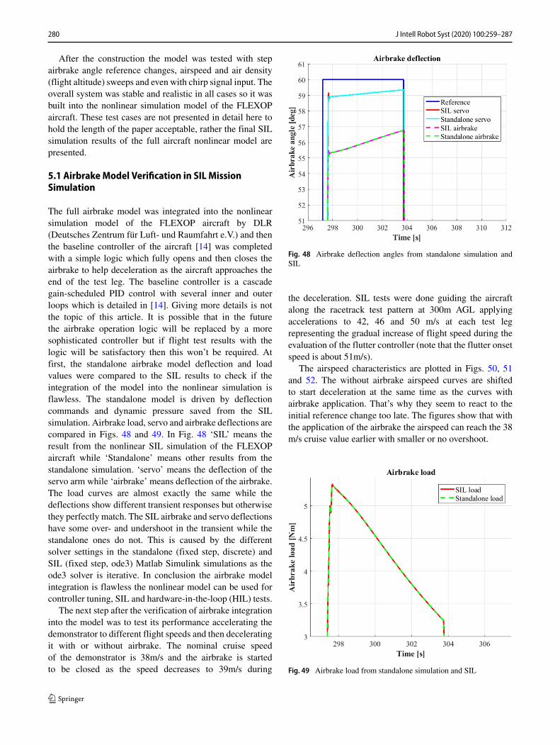
The full airbrake model was integrated into the nonlinearsimulation model of the FLEXOP aircraft by DLR(Deutsches Zentrum fur Luft- und Raumfahrt e.V.) and thenthe baseline controller of the aircraft [14] was completedwith a simple logic which fully opens and then closes theairbrake to help deceleration as the aircraft approaches theend of the test leg. The baseline controller is a cascadegain-scheduled PID control with several inner and outerloops which is detailed in [14]. Giving more details is notthe topic of this article. It is possible that in the futurethe airbrake operation logic will be replaced by a moresophisticated controller but if flight test results with thelogic will be satisfactory then this won’t be required. Atfirst, the standalone airbrake model deflection and loadvalues were compared to the SIL results to check if theintegration of the model into the nonlinear simulation isflawless. The standalone model is driven by deflectioncommands and dynamic pressure saved from the SILsimulation. Airbrake load, servo and airbrake deflections arecompared in Figs. 48 and 49. In Fig. 48 ‘SIL’ means theresult from the nonlinear SIL simulation of the FLEXOPaircraft while ‘Standalone’ means other results from thestandalone simulation. ‘servo’ means the deflection of theservo arm while ‘airbrake’ means deflection of the airbrake.The load curves are almost exactly the same while thedeflections show different transient responses but otherwisethey perfectly match. The SIL airbrake and servo deflectionshave some over- and undershoot in the transient while thestandalone ones do not. This is caused by the differentsolver settings in the standalone (fixed step, discrete) andSIL (fixed step, ode3) Matlab Simulink simulations as theode3 solver is iterative. In conclusion the airbrake modelintegration is flawless the nonlinear model can be used forcontroller tuning, SIL and hardware-in-the-loop (HIL) tests.

The next step after the verification of airbrake integrationinto the model was to test its performance accelerating thedemonstrator to different flight speeds and then deceleratingit with or without airbrake. The nominal cruise speedof the demonstrator is 38m/s and the airbrake is startedto be closed as the speed decreases to 39m/s during

Fig. 48 Airbrake deflection angles from standalone simulation andSIL

the deceleration. SIL tests were done guiding the aircraftalong the racetrack test pattern at 300m AGL applyingaccelerations to 42, 46 and 50 m/s at each test legrepresenting the gradual increase of flight speed during theevaluation of the flutter controller (note that the flutter onsetspeed is about 51m/s).

The airspeed characteristics are plotted in Figs. 50, 51and 52. The without airbrake airspeed curves are shiftedto start deceleration at the same time as the curves withairbrake application. That’s why they seem to react to theinitial reference change too late. The figures show that withthe application of the airbrake the airspeed can reach the 38m/s cruise value earlier with smaller or no overshoot.

Fig. 49 Airbrake load from standalone simulation and SIL


Fig. 50 Airspeed profiles with 42 m/s reference

Table 7 summarizes the settling times of SIL simulationregarding ±2% tolerance around the 38 m/s cruise speed(37.24− 38.76m/s, the usually applied ±5% range was toolarge with almost 40 m/s upper bound). The time gain meansthe time with which the deceleration with airbrake is shorterand so the flutter test can be longer. The distance gain isthe time gain multiplied by 38 m/s which is the minimumgained distance on the test leg. The table shows that theflutter test can be from 1.5s to as large as almost 4s longerwith airbrake application which can largely help to betterevaluate the behavior. After SIL testing the final verificationof the airbrake model is done in the next section consideringflight test results.



5.2 Flight Test Results

Real flight test results were obtained in two manual flightsin August 2019 at Munchen Oberpfaffenhofen airport. Theaircraft was manually controlled into almost straight andlevel flight and then applying constant throttle (see Fig. 60)and trying to hold the flight direction (see Fig. 53) theairbrake was manually fully opened and closed giving astaircase reference until maximum deflection (see e. g.Fig. 54) and after some time back. Straight and levelflight was targeted to give an opportunity to realisticallyevaluate the effect of the airbrake in decreasing the airspeedof the aircraft. The tests are approximately repeatable asthe similar altitude and airspeed ranges show in Table 8.Unfortunately manual control can not perfectly hold altitude(see Fig. 59) so finally the system specific energy wasused for evaluation. In the future in frame of the nextFLiPASED (see [1]) project airbrake tests are plannedwith autopilot control during 2020 which will betterbe repeatable. However, precise evaluation of airbrakeeffectiveness is not strictly required to evaluate the airbrakedynamic model itself that’s why model identification resultscan be published now.

The ranges of barometric flight altitude (h) and indicatedairspeed (V ) are shown in Table 8 and Fig. 59 shows theirrelative changes starting from the first value at activation

Table 7 Airspeed settling absolute times in SIL

Vref [m/s] 42 46 50

w/o Aibrake [s] 85.6 197.73 307.64

w. Airbrake [s] 84.1 195.06 303.85

Time gain [s] 1.5 2.67 3.79

Distance gain [m] 57 101.46 144.02


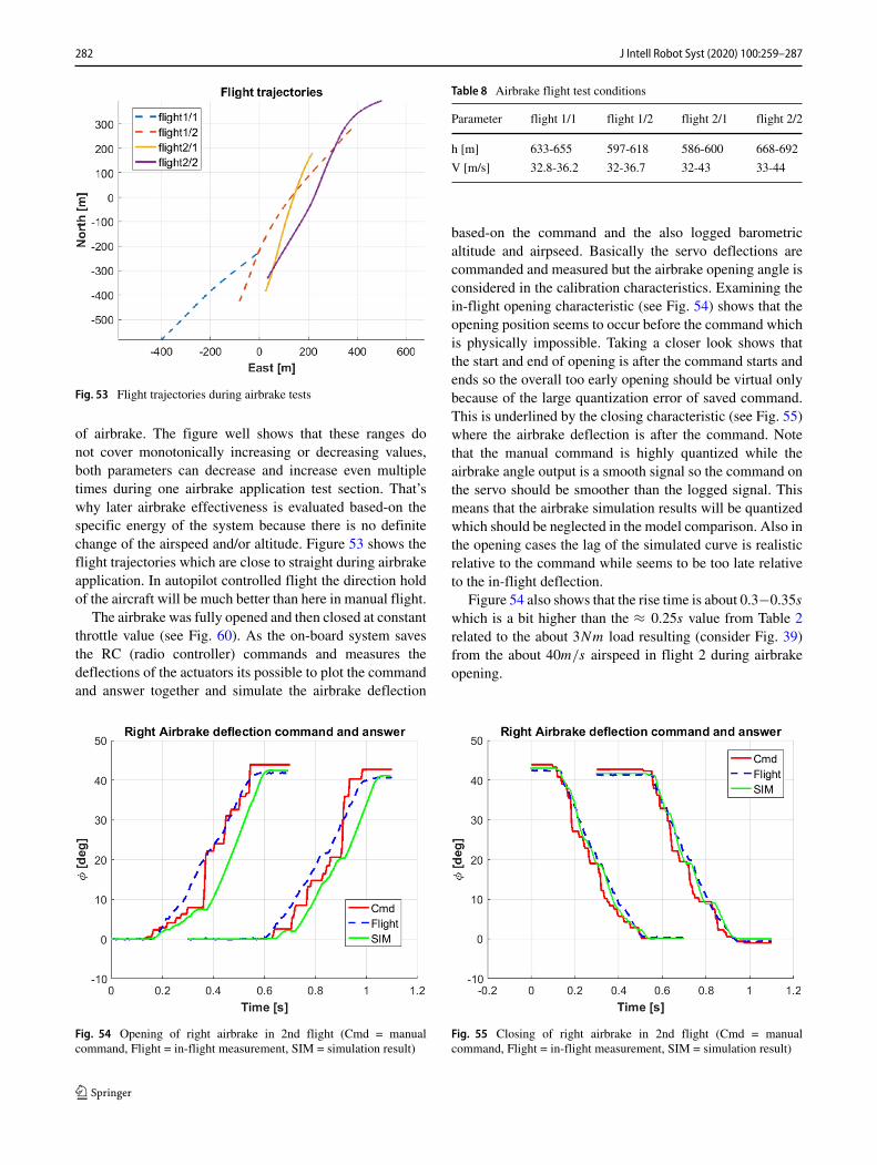
Fig. 53 Flight trajectories during airbrake tests

of airbrake. The figure well shows that these ranges donot cover monotonically increasing or decreasing values,both parameters can decrease and increase even multipletimes during one airbrake application test section. That’swhy later airbrake effectiveness is evaluated based-on thespecific energy of the system because there is no definitechange of the airspeed and/or altitude. Figure 53 shows theflight trajectories which are close to straight during airbrakeapplication. In autopilot controlled flight the direction holdof the aircraft will be much better than here in manual flight.

The airbrake was fully opened and then closed at constantthrottle value (see Fig. 60). As the on-board system savesthe RC (radio controller) commands and measures thedeflections of the actuators its possible to plot the commandand answer together and simulate the airbrake deflection

Fig. 54 Opening of right airbrake in 2nd flight (Cmd = manualcommand, Flight = in-flight measurement, SIM = simulation result)

Table 8 Airbrake flight test conditions

Parameter flight 1/1 flight 1/2 flight 2/1 flight 2/2

h [m] 633-655 597-618 586-600 668-692

V [m/s] 32.8-36.2 32-36.7 32-43 33-44

based-on the command and the also logged barometricaltitude and airpseed. Basically the servo deflections arecommanded and measured but the airbrake opening angle isconsidered in the calibration characteristics. Examining thein-flight opening characteristic (see Fig. 54) shows that theopening position seems to occur before the command whichis physically impossible. Taking a closer look shows thatthe start and end of opening is after the command starts andends so the overall too early opening should be virtual onlybecause of the large quantization error of saved command.This is underlined by the closing characteristic (see Fig. 55)where the airbrake deflection is after the command. Notethat the manual command is highly quantized while theairbrake angle output is a smooth signal so the command onthe servo should be smoother than the logged signal. Thismeans that the airbrake simulation results will be quantizedwhich should be neglected in the model comparison. Also inthe opening cases the lag of the simulated curve is realisticrelative to the command while seems to be too late relativeto the in-flight deflection.

Figure 54 also shows that the rise time is about 0.3−0.35swhich is a bit higher than the ≈ 0.25s value from Table 2related to the about 3Nm load resulting (consider Fig. 39)from the about 40m/s airspeed in flight 2 during airbrakeopening.

Fig. 55 Closing of right airbrake in 2nd flight (Cmd = manualcommand, Flight = in-flight measurement, SIM = simulation result)


The airbrake model was simulated considering the actualbarometric flight altitude and indicated airspeed values andthe manual deflection commands of the airbrake. Note thatthe maximum physical deflection of the airbrakes on theaircraft is about 45◦ in contrast to the maximum 60◦ testbench deflection. The steady state values of simulated andin-flight airbrake angles are very close to each other (max0.6◦ difference) so this does not require model refinement.

The comparison of simulated closing characteristic (asthe opening can not be taken as a precise reference) withthe in-flight one shows that the simulation with the threetime steps delay in the servo dynamics lags more than theflight data. This means that the delay could be decreasedfinally to 1 step giving results better following the flightdata (see Fig. 56). The figure also shows that the slopeof the simulated signal is a bit larger than the in-flightone. This can be possibly solved by further limiting themaximum closing speed of the servo under load. Examiningthe closing speed limits and the load resulting from in-flight dynamic pressure shows that the load is about 2Nm

and so the current maximum closing speed is −372◦/sin the simulation model. The maximum limitation of thespeed can be −340◦/s but this is very close to the currentmodel (91.3%) and does not improve significantly theperformance so finally the closing speed characteristicremained unchanged. As the airbrake closes only if theairspeed is decreased to a low value the load duringthe closing will always be small so the load dependentclosing speed will be around the above mentionedvalues.

Considering the slope of the opening in Fig. 54 in the firstcase the simulated slope is a bit larger while in the second

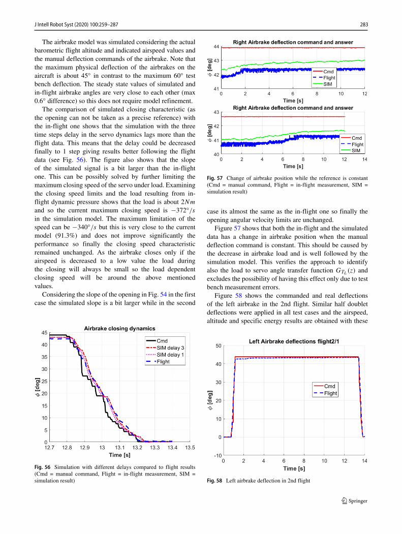
Fig. 56 Simulation with different delays compared to flight results(Cmd = manual command, Flight = in-flight measurement, SIM =simulation result)

Fig. 57 Change of airbrake position while the reference is constant(Cmd = manual command, Flight = in-flight measurement, SIM =simulation result)

case its almost the same as the in-flight one so finally theopening angular velocity limits are unchanged.

Figure 57 shows that both the in-flight and the simulateddata has a change in airbrake position when the manualdeflection command is constant. This should be caused bythe decrease in airbrake load and is well followed by thesimulation model. This verifies the approach to identifyalso the load to servo angle transfer function GTL

(z) andexcludes the possibility of having this effect only due to testbench measurement errors.

Figure 58 shows the commanded and real deflectionsof the left airbrake in the 2nd flight. Similar half doubletdeflections were applied in all test cases and the airspeed,altitude and specific energy results are obtained with these

Fig. 58 Left airbrake deflection in 2nd flight


14 to 24 seconds deflections. Figure 59 shows the changein airspeed and altitude during airbrake application. Allinitial values were shifted to zero to show the decrease orincrease of the values relative to the initial. The airspeeddecreases with about 2 m/s in the first flight and morethen 5 m/s in the second while the time horizons areabout the same. This is because in the first flight theinitial airspeeds are 34-36 m/s while in the second flightthey are about 43 m/s (see Table 8). As the drag forceof the airbrake scales quadratically with airspeed this isnot surprising as higher drag means higher deceleration.Regarding the altitude it increases in one of the cases whiledecreases in all other three. As the altitude can increase /decrease during the maneuvers its hard to estimate if thedecrease in airspeed is caused by altitude change or bythe airbrake.

To decide about this the overall energy state of theaircraft should be considered. With constant throttle andsmall changes in altitude and airspeed the thrust of thejet engine can be assumed to be almost constant and sostarting from a trimmed condition the energy content shouldnot change significantly. However, plotting the specificenergy u = gh + 1

2V2 (see Fig. 60, h is barometric

altitude and g is the gravitational constant) shows that theenergy content of the aircraft decreases so the airbrakeremoves energy from the system. As the mass of the aircraftslightly changes due to fuel consumption the specific energyis considered instead of the whole potential and kineticenergies.

As a conclusion it can be stated that the flight test dataverifies the airbrake simulation model having similar resultsin simulation then in flight so this model can be applied formore sophisticated airbrake control design and for the HILverification of any autopilot applying airbrake.

Fig. 59 Airspeed and barometric altitude during airbrake operation

Fig. 60 Throttle positions δth and specific energy u

6 Conclusion

This paper presents the modeling and system identificationof the airbrake of an unmanned experimental aircraft. Thisairbrake consists of a servo motor, a nonlinear mechanismand the aibrake flap itself. After briefly introducing thedemonstrator aircraft and summarizing the design consider-ations the system identification concept is discussed. Thenthe applied test benches are briefly described which are afull scale mock-up and a servo test bench with load motor.

From this point the work focuses on the identificationof the servo dynamics based on test bench measurementsfirst pulling out the significant nonlinearities from thesystem. These include the characterization of the loaddependent opening and closing angular velocities and theestimation of the saturation level of servo angular velocityreference input. The remaining linear part of the servodynamics was identified as a transfer function plus delayterm. As the load causes a steady-state servo angle changethis load dependent angle change was also modeled as atransfer function. This effect was verified by flight testresults so this transfer function is a required part of theairbrake model. After constructing the servo model itsverification based-on test bench measurements was done.The next step was the description and identification ofstatic characteristics. This includes the aerodynamics asdrag and normal force coefficients. The former is modeledwith a line fit against the airbrake deflection angle, thelatter is normalized and modeled as a combination of aparabola and a line again against the airbrake angle. Thena virtual servo arm is defined and its characteristics aredetermined considering the nonlinearities in the airbrakeopening mechanism. This, together with the normalizednormal force coefficient gives the relation between thedynamic pressure, airbrake opening angle and servo load


torque. After generating these the airbrake opening angle- airspeed - servo load torque characteristics are plottedfor the whole operational range of the aircraft. Theoverall precision of this modeling resulted between 6 to1 percent depending on the opening angle (compared tothe calculated tabular data). These characteristics made itpossible to select the required measurements for systemidentification which represent operational cases from a setof test bench measurements (opening angle range and loadrange sweep). Finally, the servo angle to airbrake angleand the reverse conversion characteristics were calculatedby fitting polynomials and the angle dependent stiffnessof the opening mechanism was also characterized. Beforeconstruction of the whole airbrake model the effect ofopening mechanism stiffness and airbrake inertia on thedynamics was examined. It has turned out that this can causeoscillations only on very high frequencies which are outsidethe planned operating range and estimated bandwidth of theairbrake.

The whole airbrake simulation model was first checkedin Monte-Carlo simulation with several angle references,airspeeds and flight altitudes and showed realistic results.Then, the airbrake model was integrated into the nonlinearsimulation model of the FLEXOP demonstrator aircraft andits effect on the deceleration characteristics was examinedconsidering software-in-the-loop trajectory tracking witha baseline controller. It has turned out that airbrakeapplication can gain 1.5 to 4 seconds additional time to testthe flutter controller of the aircraft.

Finally, in-flight manual test of the airbrake was done inAugust 2019. Comparing the simulation model with the in-flight results has shown that the delay of the servo modelcan be decreased (from 3 time steps to 1) but otherwisethe model well covers the opening, the closing and eventhe load change characteristics of the real airbrake. As inmanual flight there is no precise altitude hold but the throttleand so the thrust was approximately constant the specificenergy of the aircraft was examined during the applicationof the airbrake. This shows that the airbrake decreasedoverall system energy in all of the cases so its application indeceleration is advantageous.

Acknowledgements The authors gratefully acknowledge the contribu-tion of Matthias Wuestenhagen at Deutsches Zentrum fur Luft- undRaumfahrt e.V. (DLR) Institut fur Systemdynamik und Regelungstech-nik (RMC-SR-FLS) who integrated the airbrake simulation model intothe nonlinear model of the FLEXOP aircraft.

The authors gratefully acknowledge the help of Tamas Luspay(senior research fellow, SZTAKI) in simulating the airbrake dynamicstogether with the baseline controller.

The authors gratefully acknowledge the contribution of Instituteof Aircraft Design, Department of Mechanical Engineering, TechnicalUniversity of Munich flight test team (Christian Roessler, FabianWiedemann, Sebastian Koeberle, Julius Bartasevicius and DanielTeubl) with executing the flight tests.

Funding Information Open Access funding provided by ELKHInstitute for Computer Science and Control.

Compliance with Ethical Standards

Conflict of interests The authors declare that they have no conflict ofinterest.

Open Access This article is licensed under a Creative CommonsAttribution 4.0 International License, which permits use, sharing,adaptation, distribution and reproduction in any medium or format, aslong as you give appropriate credit to the original author(s) and thesource, provide a link to the Creative Commons licence, and indicateif changes were made. The images or other third party material in thisarticle are included in the article’s Creative Commons licence, unlessindicated otherwise in a credit line to the material. If material is notincluded in the article’s Creative Commons licence and your intendeduse is not permitted by statutory regulation or exceeds the permitteduse, you will need to obtain permission directly from the copyrightholder. To view a copy of this licence, visit http://creativecommons.org/licenses/by/4.0/.

Appendix

φ − cD fit:

cD(φ) = 0.88 · φ[rad]φ − c′

N fit:

c′NL

(φ) = φ2[rad2]+1.8706φ[rad] if 0≤φ<0.6962rad

c′NH

(φ) = 0.0514φ[rad] + 1.7512 if 0.6962rad ≤ φ (7)

φ − sa fit:

sa(φ)[m] = −0.02735φ5[rad5] + 0.09069φ4[rad4] − 0.11428φ3[rad3]+0.071245φ2[rad2] − 0.02437φ[rad] + 0.006 (8)

α − φ curve:

φ(α)[rad] = −0.01864α3[rad3] + 0.213425α2[rad2] + 0.20056α[rad]

φ − α curve:

α(φ)[rad] = −1.83448φ4[rad4] + 5.03271φ3[rad3]−5.28037φ2[rad2] + 3.9602φ[rad] (9)

Stiffness formula:

kφ = 1383.097φ3[rad3]−3028.264φ2[rad2]+1764.837φ[rad]+45.722

System dynamics from angular velocity reference toangular velocity:

Gsys(z) = 1.039

1 + 0.0149z−1 + 0.238z−2 − 0.2361z−3


http://creativecommons.org/licenses/by/4.0/

http://creativecommons.org/licenses/by/4.0/

System dynamics from delayed load to angle:

GTL(z) = −0.002181

1 − 0.5267z−1

References

1. Flight phase adaptive aero-servo-elastic aircraft design methods.cordis.europa.eu/project/id/815058

2. Flutter Free Flight Envelope Expansion for Economical Perfor-mance Improvement (2015). https://flexop.eu/

3. Adam, E., Guestrin, E.: Identification and robust control ofan experimental servo motor. ISA Transactions 41(2), 225–234(2002). https://doi.org/10.1016/S0019-0578(07)60082-2. http://www.sciencedirect.com/science/article/pii/S0019057807600822

4. Anastasopoulos, L., Hornung, M.: Design of a real-time test benchfor UAV servo actuators. AIAA AVIATION Forum. AmericanInstitute of Aeronautics and Astronautics. https://doi.org/10.2514/6.2018-3735 (2018)

5. Batista, J., Sousa, K., Nunes, J.L., Sousa, R.S., The, G.A.P.:Identification of the parameters of a ac servomotor using geneticalgorithm. https://doi.org/10.5281/zenodo.1100140 (2015)

6. Davies, H., Kirk, F.: A resume of aerodynamic data on airbrakes.Tech. Rep., Aeronautical Research Council, Ministry of Supply(1951)

7. Grote, K.H., Feldhusen, J.: Dubbel: Taschenbuch Fur DenMaschinenbau, Auflage, vol. 22. Springer, Berlin (2007)

8. Ishak, N., Abdullah, N.I., Rahiman, M.H.F., Samad, A.M., Adnan,R.: Model identification and controller design for servomotor. In:2010 6th International Colloquium on Signal Processing and itsApplications, pp. 1–4 (2010). https://doi.org/10.1109/CSPA.2010.5545294

9. Koerner, D.: Experimental System Identification of an ElectricActuated Airbrake System for the FLEXOP Research UAV.Bachelor Thesis, Institute of Aircraft Design Technical Universityof Munich (2018)

10. KST: X30-12-1500 Technical Specification (2018)11. Ljung, L.: System Identification: Theory for the User. Prentice

Hall information and system sciences series. Prentice Hall PTR.https://books.google.hu/books?id=nHFoQgAACAAJ (1999)

12. Ortiz, X., Rival, D.E., Wood, D.W.: Forces and moments on flatplates of small aspect ratio with application to PV wind loads andsmall wind turbine blades. Energies 8(4), 1–16 (2015)

13. Piatek, M.: Identification of the servo motor used in the walkingrobot. AUTOMATYKA 14(1) (2010)

14. Pusch, M., Ossmann, D., Luspay, T.: Structured control designfor a highly flexible flutter demonstrator. Aerospace 6(3).https://doi.org/10.3390/aerospace6030027. https://www.mdpi.com/2226-4310/6/3/27 (2019)

15. Sendner, F.M., Stahl, P., Roessler, C., Hornung, M.: Designing anuav propulsion system for dedicated acceleration and decelerationrequirements. AIAA AVIATION Forum. American Instituteof Aeronautics and Astronautics. https://doi.org/10.2514/6.2017-4105 (2017)

16. Sendner, F.M., Stahl, P., Roessler, C., Hornung, M.: Design andtesting of an electric actuated airbrake for dynamic airspeedcontrol of an unmanned aeroelastic research vehicle. AIAAAVIATION Forum. American Institute of Aeronautics andAstronautics. https://doi.org/10.2514/6.2018-3194 (2018)

17. Takarics, B., Patartics, B., Luspay, T., Vanek, B., Roessler, C.,Bartasevicius, J., Koeberle, S.J., Hornung, M., Teubl, D., Pusch,M., Wustenhagen, M., Kier, T.M., Looye, G., Bauer, P., Med-daikar, Y.M., Waitman, S., Marcos, A.: Active flutter mitigationtesting on the FLEXOP demonstrator aircraft. In: AIAA Scitech

2020 Forum (2020). https://doi.org/10.2514/6.2020-1970. https://arc.aiaa.org/doi/abs/10.2514/6.2020-1970

18. Wada, T., Ishikawa, M., Kitayoshi, R., Maruta, I., Sugie, T.:Practical modeling and system identification of R/C servo motors.In: 2009 IEEE Control Applications, (CCA) Intelligent Control,(ISIC), pp. 1378–1383 (2009). https://doi.org/10.1109/CCA.2009.5280987

Publisher’s Note Springer Nature remains neutral with regard tojurisdictional claims in published maps and institutional affiliations.

Peter Bauer received his M.Sc. and Ph.D in Mechanical Engineering(Aerospace Engineering) in 2005 and 2013, respectively, at BudapestUniversity of Technology and Economics, Budapest, Hungary. He isa Senior Research Fellow at the Institute for Computer Science andControl, Budapest, Hungary. He is quality manager in EU H2020projects (Flexop, FLiPASED) and was actively involved in the VISIONEU H2020 project regarding camera-based landing (IMU-cameradata fusion) and camera, GPS, ILS system fault detection research.His other research fields cover state and parameter estimation,tracking control design, aircraft autopilot and sense and avoid systemdevelopment. He also designs and coordinates flight test experiences.

Lysandros Anastasopoulos earned his B.Sc. and M.Sc. in Mechani-cal Engineering at the Technical University of Darmstadt. After a shorttime in the industry, he worked as a research assistant at the TechnicalUniversity of Munich in the field of real-time aircraft systems testing.He is currently employed in Switzerland’s aviation industry and col-laborates with the National Technical University of Athens in the fieldof non-linear dynamics.

Franz-Michael Sendner received his M.Sc. and B.Sc. degree inAerospace Engineering from Technical University of Munich (TUM).He joined the Institute of Aircraft Design of TUM as a researchscientist in 2016, being in charge of the propulsion and airbrake systemof the FLEXOP demonstrator. In 2018 Franz Sendner joined FACC’sResearch & Technology Department, starting with the demonstratorwing manufacturing and currently working on integral design basedsolutions for wing moveables of transport aircraft.

Mirko Hornung received his doctorate in aeronautical engineeringfrom the University of the Bundeswehr (Federal Armed Forces)in Munich. His thesis on reusable space transport systems wasawarded a research prize in 2003. From 2003 to 2009 he workedat EADS Defence and Security (today: Airbus Defence and Space)on propulsion system integration, program management and businessdevelopment. In his last position, he was responsible for the initialdevelopment of future airvehicles and unmanned aerial systems. Hewas appointed Professor for Aircraft Design at TUM in 2010 and ishead of the Institute of Aircraft Design and his research is in the area ofaircraft design, integration, and evaluation. His focus is on conceptualaircraft design and the theoretical and experimental evaluation ofoverall system technologies under operational conditions. He isExecutive Director Research and Technology of Bauhaus Luftfahrte.V., a non-profit organization and an internationally oriented thinktank. Mirko Hornung is senior member of AIAA, member of theexecutive board of Deutsche Gesellschaft fur Luft- und Raumfahrt(DGLR), member of the bavAIRia advisory board and member of theTransport Advisory Group for H2020.

Balint Vanek currently deputy head of the research laboratory SCL atSZTAKI, obtained his Msc from Budapest University of Technologyand Economics in 2003 and the PhD from University of Minnesota in


cordis.europa.eu/project/id/815058

https://flexop.eu/

https://doi.org/10.1016/S0019-0578(07)60082-2

http://www.sciencedirect.com/science/article/pii/S00190578076 00822

http://www.sciencedirect.com/science/article/pii/S00190578076 00822

https://doi.org/10.2514/6.2018-3735

https://doi.org/10.2514/6.2018-3735

https://doi.org/10.5281/zenodo.1100140

https://doi.org/10.1109/CSPA.2010.5545294

https://doi.org/10.1109/CSPA.2010.5545294

https://books.google.hu/books?id=nHFoQgAACAAJ

https://doi.org/10.3390/aerospace6030027

https://www.mdpi.com/2226-4310/6/3/27

https://www.mdpi.com/2226-4310/6/3/27

https://doi.org/10.2514/6.2017-4105

https://doi.org/10.2514/6.2017-4105

https://doi.org/10.2514/6.2018-3194

https://doi.org/10.2514/6.2020-1970

https://arc.aiaa.org/doi/abs/10.2514/6.2020-1970

https://arc.aiaa.org/doi/abs/10.2514/6.2020-1970

https://doi.org/10.1109/CCA.2009.5280987

https://doi.org/10.1109/CCA.2009.5280987

2008. Prior to working at SZTAKI he was a senior research scientist atHoneywell Aerospace Advanced Technology. Balint’s research inter-est includes guidance, navigation and control related to safety aspectsof both manned and unmanned aerial vehicles, including fault detec-tion and reconfigurable control of aerospace systems, unmanned aerialvehicles (UAV) and their insertion into the common airspace, as wellas aeroservoelastic behavior of advanced aircraft configurations. He isthe coordinator of the FLEXOP and FLiPASED EU H2020 projects.


Documents

Identification and Modeling of the Airbrake of an