Identification and Estimation with Partial Respondents and

1

Identification and Estimation with Partial Respondents and

Anchoring Effects

Bertrand Melenberg a, Arthur van Soest b and Rosalia Vazquez-Alvarez c,*, a Centre For Economic Research, (CentER), Tilburg University, The Netherlands

b RAND Corporation, Santa Monica and Centre for Economic Research, (CentER), Tilburg University c Swiss Institute for International Economics and Applied Economic Research (SIAW), University of St.Gallen

This version: February, 2008*

Abstract

Household surveys often suffer from nonresponse on variable such as income, savings or wealth. The work

by Charles F. Manski in the 1990s shows how bounds on conditional quantiles on the variable of interest can be

derived, allowing for any type of non-random item nonresponse. The width between these bounds can be reduced

using follow up questions in the form of unfolding brackets for initial non-respondents. However, evidence from

both the psychology and economic literature suggest that such design is vulnerable to anchoring effects. In this paper

Manski’s bounds are extended to incorporate information provided by bracket respondents allowing for three

alternative nonparametric assumptions on anchoring. The new bounds are applied to earnings in the 1996 wave of

the Health and Retirement study. The results show that introducing categorical questions in the form of unfolding

designs can be useful to increase the precision of the bounds, even if anchoring is allowed for.

Keywords: Identification, item nonresponse, survey design, anchoring effects, unfolding bracket design

JEL – Classification : C13, C14, C81, D31

* Adrress for correspondence: SIAW, University of St.Gallen, Bodanstrasse, 8, CH-9000, [email protected]

Email: [email protected], [email protected], [email protected]

We are grateful to the ISSC policy research group (Dublin University College) and seminar participants at the University of St.Gallen. We are

also indebt to Michael Lechner for providing very valuable advice. This paper draws from an initial discussion paper entitled ‘Nonparametric

bounds in the presence of item nonresponse, unfolding brackets and anchoring’, CentER discussion paper series, 01-57.

2

1 Introduction Household surveys are often plagued by item nonresponse on certain variables relating to

quantities. For example, in the 1996 wave of the Health and Retirement Study (HRS), a USA panel often

used to study socio-economic behaviour of the elderly, 12% of the weighted sample that declare a status

of paid employee do not declare their earnings when asked for an exact amount. One way to deal with

nonresponse is to use information from full respondents (i.e., assuming nonresponse exogeneity). The

problem is that biased estimates of the population parameters may result if nonresponse is related to the

variable under study thus leading to the classic selection problem (see the seminal work by Manski, 1990,

1994 or more recent surveys in item nonresponse by Mason et al., 2002). Alternative methods to that of

exogeneity (e.g., imputation procedures such as those suggested in Rubin, 1987) still require the use of

alternative distributional assumptions that cannot be tested with the same data used in the process of

estimation.

Manski (as leading examples, see Manski 1989, 1990, 1994, 1995, 1997, 2000) shows how

bounds on conditional quantiles of the variables of interests can be derived, allowing for any type of non-

random nonresponse behaviour. Manski’s framework is intuitively appealing, easy to apply, and very

flexible, but has the drawback that the resulting bounds are often too wide to draw meaningful economic

conclusions. In Manski’s framework the precision with which features of the distribution (e.g., its

quantiles) can be determined, i.e., the width between the bounds, depends on the probability of

nonresponse. If item nonresponse is substantial, the approach cannot lead to accurate estimates of the

parameters of interest without additional information or additional assumptions. A combination of

informative data sets and weak data-driven assumptions are often effective at tightening the bounds (for

empirical illustrations that follow this approach, see for example, Ginther (2000), Manski and Pepper

(2000), Pepper (2000) and Pepper (2003)).

Data collection strategies can also reduce the problem of item nonresponse even before the data

reaches the user. For example, the use of an unfolding bracket designs to elicit partial information from

initial item non-respondents. These designs drive individuals through a sequence of questions that sort

individual’s undisclosed amount inside a particular category in the support of the variable that suffers

from nonresponse. This is done by prompting initial non-respondents to react to a sequence of ‘bids’. At

each bid the respondent has to reveal if they perceive the otherwise undisclosed amount to be greater (or

not) than the bid. The inclusion of bracket designs is an effective way to reduce the problem of initial item

nonresponse. Following with the example above (HRS, 1996) 73.4% of the weighted initial non-

respondents to earnings answer the unfolding bracket design thus effectively reducing full nonresponse

rate from 12% to 3% in the complete weighted sample.

3

In general, the use of categorical questions is motivated because it is thought that rather than the

characteristics of the question, it is personal characteristics and cognitive factors (e.g., confidentiality

reasons) what drives nonresponse behaviour (for issues relating to survey response behaviour see for

example, Borgers and Hox, 2001, Juster and Smith, 1997, Mason et al., 2000, Rabin, 1998, or Tourangeau

et al., 2000). The problem with unfolding bracket designs is that these may induce ‘anchoring effects’, a

phenomenon well documented in the psychology literature (see, for example, Tversky and Kahneman,

1974, Swizer and Sniezek, 1991, Jacowitz and Kahneman, 1995). In the context of the present paper,

anchoring effects can be explained in the presence of bids from the unfolding design. Individuals may or

may not be uncertain about the undisclosed amount (e.g., some individuals genuinely do not know the

amount and other prefer not to disclose it), but different sequences of bids can induce different sets of

answers if the bids act as ‘anchors’ and responses are driven in the direction of the bids. Hurd et al. (1998)

show the existence of anchoring on questions relating to wealth and consumption using an experimental

module from the 1996 wave of the HRS. Other experimental studies show that even if the anchor is

arbitrary and uninformative this can have large effects on the responses behaviour of the sample as is the

case in the experimental set up of Jacowitz and Kahneman (1995). Alternative parametric models for

anchoring are introduced by Cameron and Quiggin (1994) and Herriges and Shogren (1996).

This paper extends the approach by Manski, incorporating the information provided by the

bracket respondents and allowing for anchoring effects with three distinct nonparametric assumptions on

anchoring. These assumptions draw from Hurd et al. (1998), Jacowitz and Kahneman (1995) and Herriges

and Shogren (1996). The bounds are applied to earnings in the 1996 wave of the Health and Retirement

Study. The results show that the categorical questions can be useful to increase precision of the bounds,

even if anchoring is allowed for. They also help to improve the power of statistical tests for equality of

earnings quantiles in sub-populations. This is shown by comparing bounds on the quantiles of earnings

between genders. The bounds which take account of bracket information can detect differences which are

not revealed by estimated bound based upon full respondents’ information only. We also use the

bounding interval to validate the assumptions underlying an imputation procedure on earnings.

The paper is organized as follows. Section 2 derives five sets of bounds: the first ignores the

presence of partial respondents; the other four allow for partial respondents but differ in the interpretation

of anchoring effects. Section 3 describes the estimation process. Section 4 describes the data used in the

empirical example and illustrates the bounds derived in Section 2 testing for earnings equality between

genders. Section 5 concludes.

4

2 Theoretical framework

2.1 Worst case bounds: no bracket respondents

Manski (1989) provides the basic set up for worst case bounds on the distribution of some

outcome Y at a given y∈ conditional on a set of covariates kX x= ∈ . The data we observe is cross-

sectional data for a sample of size n representative of the underlying population. We assume all variables

in the covariate set to be free from unit and item nonresponse.1 Furthermore, all reported (exact) values on

Y and X are assumed to be correct so that misreporting of exact amounts is not an issue in this analysis.

Let FR and NR indicate, respectively, full response and full nonresponse on Y . With this, the

conditional distribution function of Y given x X∈ can be partition as follows:

( | ) ( | , ) ( | ) ( | , ) ( | )F y x F y x FR P FR x F y x NR P NR x= + (1)

The assumptions imply that ( | , )F y x FR , ( | )P FR x and ( | )P NR x are identified for all x X∈ .

The sample analogues can be estimated, for example, using some nonparametric regression technique.

The identification problem arises because ( | , )F y x NR is not revealed by the sampling process. Assuming

conditional (on X ) exogeneity solves the identification problem because it implies that

( | , ) ( | , )F y x FR F y x NR= , i.e., conditional on X response behaviour is independent of Y . In general,

however, response behaviour is related to Y and ( | , )F y x NR is not identified, so that ( | )F y x in (1) is

not identified either. Without additional assumptions, all that is known about ( | , )F y x NR is that it is

naturally bounded between 0 and 1. Applying this to (1) gives,

( | , ) ( | ) ( | ) ( | , ) ( | ) ( | )F y x FR P FR x F y x F y x FR P FR x P NR x≤ ≤ + (2)

Expression (2) illustrates Manski’s worst case bounds for the conditional distribution function. The width

between bounds is ( | )P NR x , thus, a low nonresponse rate can only improve the identification region for

any x X∈ . Additional weak data-driven assumptions can tighten the bounds as is the case of

monotonicity and exclusion restrictions (see Manski, 1994, 1995).

2.2 Partial Information from an Unfolding bracket Design

In this paper bounds in (2) are extended to incorporate information from a follow-up unfolding

bracket design. In this type of design initial non-respondents are faced with successive questions each

1 For an interpretation of bounds with covariates nonresponse see Horowitz and Manski (1995,1998) and for the

extension to cover covariates unfolding bracket response with anchoring see Vazquez-Alvarez (2006)

5

containing different amounts $B that reflect values in the support of Y . The aim is to elicit partial

information by asking initial non-respondents if the otherwise undisclosed amount is grater (or not) than

the bid $B .2 Presenting successive bids conditional on previous answers helps to classify the unknown

quantity in some category in the support of Y . It is possible that in the presence of an unfolding bracket

design a fraction of initial non-respondents still provide no information on the undisclosed amount: this is

the case when the answer is ‘don’t know’ or ‘refuse to respond’ at the first bid in the sequence.3 Thus,

even in the presence of follow-up questions the probability ( ) 0P NR > remains. Once a decision is made

to answer the first bid, individuals may or may not complete the sequence of bids. Those who complete

the sequence are defined as complete bracket respondents (CBR) whereas incomplete bracket respondents

(IBR) are those who declare ‘don’t know’ or ‘refuse to respond’ at some point before the sequence is over.

Notice that in both cases – CBR and IBR –, the nature of information they provide is identical, i.e., both

types provide partial information that determines a category in the support of Y . The two types differ

because their answers define different sets of categories in Y . We want to derive bounding intervals

introducing partial information through an unfolding bracket design, and this can be done without loss of

generality by assuming that all bracket respondents are CBR. At the end of this section we go back to look

at the effect of further introducing information from IBR within the derived bounds. With this, three types

of respondents can be distinguished; full respondents ( )FR , full non-respondents ( )NR and bracket

respondents ( )BR defined as those who complete the sequence of questions in the unfolding bracket

design. Allowing for these subgroups of respondents, the following partition applies:

( | ) ( | , ) ( | ) ( | , ) ( | ) ( | , ) ( | )F y x F y x FR P FR x F y x BR P BR x F y x NR P NR x= + + (3)

The sampling process is informative on ( | , )F y x FR , ( | )P FR x , ( | )P BR x and ( | )P NR x while

the assumption ( | , ) [0,1]F y x NR ∈ still applies. The new issue is what the answers to an unfolding

bracket design say about ( | , )F y x BR . As described in Section 1, anchoring effects may be induced when

individuals’ answers are influenced by the wording in the question. To allow for this possibility we derive

bounds on ( | )F y x first ignoring and then allowing for potential anchoring effects on ( | , )F y x BR .

2 All questions in an unfolding bracket design follow a unique direction. For example, when the first question in the design is

given as ‘is the amount greater than B?’, the second and follow up questions also refer to ‘greater than’ although the amounts differ to become above or below B.

3 Survey response often distinguish between types of nonresponse, for example, nonresponse with ‘don’t know’ (that might be due to true inability to retrieve information) and ‘refuse’ to respond, possibly associated with the information that the interviewer tries to elicit (see, for example, Tourangeau et al, 2000). In our case it is important to notice that both types (‘don’t know’ or ‘refuse’) contribute equally to the uncertainty due to item nonresponse, thus to the width between upper and lower bounds. It is therefore not an issue to distinguish between them.

6

2.3 Partial Information with no anchoring effects

Let κ be a binary outcome so that 1κ = indicates a ‘yes’ answer and 0κ = indicates a ‘no’

answer to a given question. An unfolding bracket design implies that a non-respondent to an initial open-

ended question faces a sequence of questions of the following nature:

( 1 , 2 ,..., ( 1) )Is the amount greater than j| ?where

j: j bid, j=1,....,J

B B B jB

B th

κ κ κ= = − =

(4)

The bid in (4) implies that at each round of the design the bid faced by an individual is conditional

on the individual’s previous answers; for CBR the indicator κ can take only two values 0 and 1. Thus,

with J bids ( ){ }min( ),( | 1 ... ( 1) ),...., | 1 ... ( 1) ,max( )Y BJ B B J NO BJ B B J YES Y= = − = = = − = defines all

possible conditional bids in the support of Y . Assuming all bracket respondents face an equal number of

bids and all respondents complete the sequence, the result is a set of 2J categories in the support of the

variable that suffers from nonresponse. These 2J categories are consecutively paired and each pair is

associated with either κ =0 or κ =1, the two possible answers to the last bid faced by individuals, a bid

reflecting an amount that depends on each individual’s previous answers. To simplify notation let Bτ

represent ( | 1 , 2 , ..., ( 1) )B Bj B B B jτ κ κ κ= = = = − = for any j J∈ . Assume that Bτ is the last bid faced

by some initial non-respondent that has completed the sequence: answering 1κ = to Bτ leads to a lower

limit in one of the 2J categories if Bτ is the last bid. Alternatively, if the answer is 0κ = the same bid

acts as an upper limit in the preceding category. With this, we can define the support of Y in terms of

resulting categories: { }1 1, 2 1 1min( ) max( )[ , ), [ ), ..., [ , ),[ , )..., [ , )TY YY B B B B B B B Bτ τ τ τ− += with subscript implying

ordinal numbers.

Our aim is to interpret the information resulting from a sequence of ‘yes’ ( 1)κ = and ‘no’ ( 0)κ =

answers in the bounding interval’s framework. Let Qτ indicate the outcome from a sequence of κ

answers to questions in (4) so that τ implies a route that leads to the j th− bid conditional on some

combined set of answers to all other ( 1)j − preceding bids, [1, ]j J∈ . Thus, τ stands as a sequence of

numbers so that { } { }1 2 1, , , ,..., , 0,1 , [1, ]j j jQ j j Jτ τ κ κ κ κ− −⇒ = ∈ summarizes all possible combinations of

answers to the conditional bid ( )| 1, 2,... ( 1)B Bj B B B jτ = − within the unfolding design. For example,

311Q results from { } { }2 13; 3, , 3,1,1j τ κ κ= ⇒ = to indicate that individuals face a 3rd bid ( 3B )

following a ‘yes’ answer to (4) for each of the two sequential bids and1 2B B , thus 311Q Qτ = implies a

question which refers to 311B Bτ = . If an answer is such that 311 1Q = , this means that the respondent

7

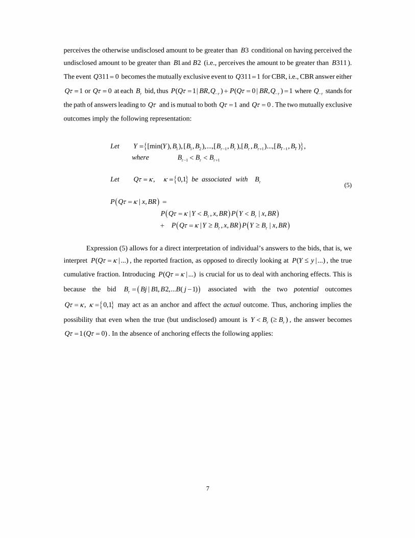
perceives the otherwise undisclosed amount to be greater than 3B conditional on having perceived the

undisclosed amount to be greater than and1 2B B (i.e., perceives the amount to be greater than 311B ).

The event 311 0Q = becomes the mutually exclusive event to 311 1Q = for CBR, i.e., CBR answer either

1Qτ = or 0Qτ = at each Bτ bid, thus ( 1| , ) ( 0 | , ) 1P Q BR Q P Q BR Qτ ττ τ− −= + = = where Q τ− stands for

the path of answers leading to Qτ and is mutual to both 1Qτ = and 0Qτ = . The two mutually exclusive

outcomes imply the following representation:

{ }

{ }

( )( ) ( )

( ) ( )

1 1 2 1 1 1

1 1

[min( ), ), [ , ),...,[ , ),[ , )...,[ , ) ,

, 0,1

| ,

| , , | ,

| , , | ,

T TLet Y Y B B B B B B B B Bwhere B B B

Let Q be associated with B

P Q x BR

P Q Y B x BR P Y B x BR

P Q Y B x BR P Y B x BR

τ τ τ τ

τ τ τ

τ

τ τ

τ τ

τ κ κ

τ κ

τ κ

τ κ

− + −

− +

=

< <

= =

= =

= < <

+ = ≥ ≥

(5)

Expression (5) allows for a direct interpretation of individual’s answers to the bids, that is, we

interpret ( | ...)P Qτ κ= , the reported fraction, as opposed to directly looking at ( | ...)P Y y≤ , the true

cumulative fraction. Introducing ( | ...)P Qτ κ= is crucial for us to deal with anchoring effects. This is

because the bid ( )| 1, 2,... ( 1)B Bj B B B jτ = − associated with the two potential outcomes

{ }, 0,1Qτ κ κ= = may act as an anchor and affect the actual outcome. Thus, anchoring implies the

possibility that even when the true (but undisclosed) amount is ( )Y B Bτ τ< ≥ , the answer becomes

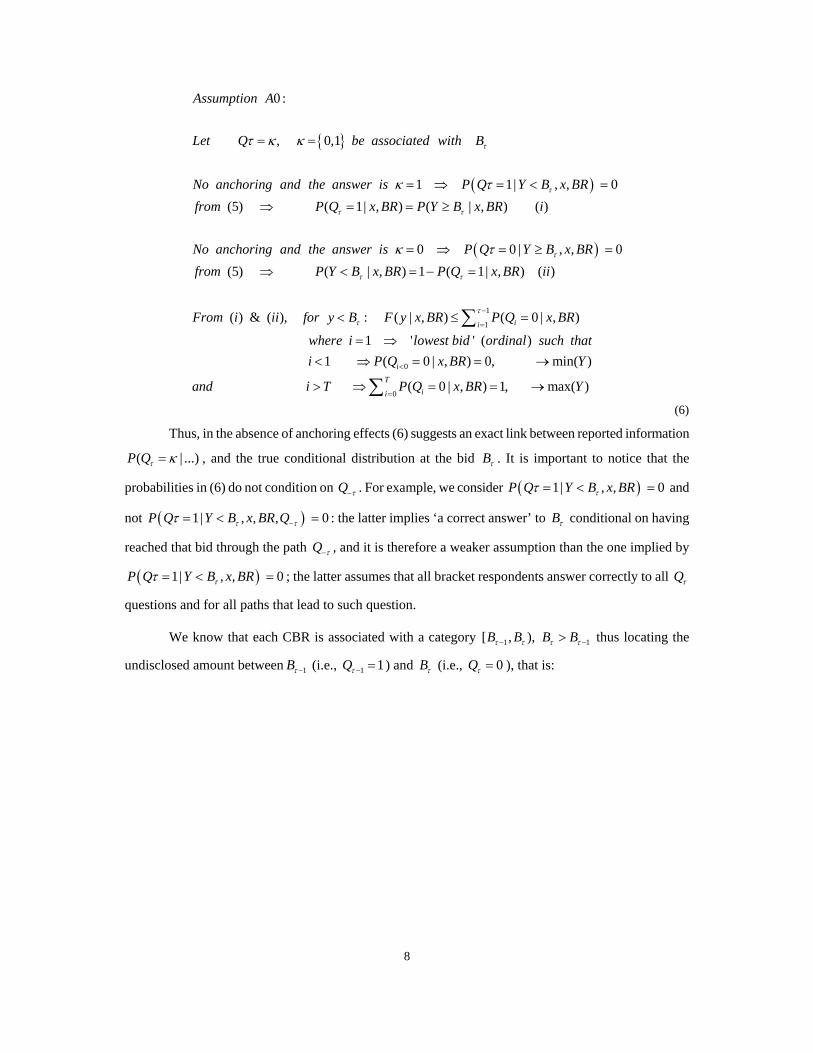
1( 0)Q Qτ τ= = . In the absence of anchoring effects the following applies:

8

{ }

( )

( )

0 :

, 0,1

1 1| , , 0(5) ( 1| , ) ( | , ) ( )

0 0 | , , 0(5) ( | , ) 1 (

Assumption A


No anchoring and the answer is P Q Y B x BRfrom P Q x BR P Y B x BR i

No anchoring and the answer is P Q Y B x BRfrom P Y B x BR P Q

τ

τ

τ τ

τ

τ τ

τ κ κ

κ τ

κ τ

= =

= ⇒ = < =

⇒ = = ≥

= ⇒ = ≥ =

⇒ < = − =

1

1

0

0

1| , ) ( )

( ) & ( ), : ( | , ) ( 0 | , )

1 ' ' ( )1 ( 0 | , ) 0, min( )

( 0 | , ) 1, max( )

ii

i

Tii

x BR ii

From i ii for y B F y x BR P Q x BR

where i lowest bid ordinal such thati P Q x BR Y

and i T P Q x BR Y

ττ

−

=

<

=

< ≤ =

= ⇒< ⇒ = = →

> ⇒ = = →

∑

∑ (6)

Thus, in the absence of anchoring effects (6) suggests an exact link between reported information

( | ...)P Qτ κ= , and the true conditional distribution at the bid Bτ . It is important to notice that the

probabilities in (6) do not condition on Q τ− . For example, we consider ( )1| , , 0P Q Y B x BRττ = < = and

not ( )1| , , , 0P Q Y B x BR Qτ ττ −= < = : the latter implies ‘a correct answer’ to Bτ conditional on having

reached that bid through the path Q τ− , and it is therefore a weaker assumption than the one implied by

( )1| , , 0P Q Y B x BRττ = < = ; the latter assumes that all bracket respondents answer correctly to all Qτ

questions and for all paths that lead to such question.

We know that each CBR is associated with a category 1 1[ , ),B B B Bτ τ τ τ− −> thus locating the

undisclosed amount between 1Bτ − (i.e., 1 1Qτ − = ) and Bτ (i.e., 0Qτ = ), that is:

9

1

1

1 1

11 1

1

[ , )0 1,

(6) : 1 0 :

: ( | , ) ( 0 | , )

0

: ( | , ) ( 0 | , )

[

ii

ii

Let B B define a category in Y resulting from partial respondentssuch that Q and Q

From Q Q defined

for y B F y x BR P Q x BR

Q

for y B F y x BR P Q x BR

For y B

τ τ

τ τ

τ τ

ττ

τ

ττ

τ

−

−

− −

−− =

=

= =

= ⇒ =

⇒ < ≤ =

=

⇒ < ≤ =

∈

∑

∑1

11, 1,1 1

1, 1,

, )

( 0 | , ) ( | , ) ( 0 | , )

min( ) 0, max( ) 1i ii i

B

L P Q x BR F y x BR U P Q x BR

where L U

τ

τ ττ τ τ τ

τ τ τ τ

−

−− −= =

− −

= = ≤ ≤ = =

= =∑ ∑

(7)

The result in (7) implies cumulative bounding interval for the unknown ( | , )F y x BR at each of

the resulting categories from an unfolding bracket design. Clearly, (7) also defines a range of values if we

are looking at some partition ory B y B≥ ≤ in the support of Y as long as B is one of the conditional

bids in the sequence. Bounds on ( | , )F y x BR given by (7) ignore anchoring effects.

2.4 Partial Information allowing for anchoring effects

Anchoring effects implies that answers to (4) could be affected by the information contained in

the bids, i.e., the bids act as an ‘anchor’ and information from partial respondents identifies the

conditional distribution of Y possibly with bias due to anchoring effects. In practical terms anchoring

implies that partial respondents may classify the otherwise undisclosed y Y∈ in 1[ , )B Bτ τ− when in fact

1[ , )y B Bτ τ−∈/ , thus, ( )i and ( )ii in (6) no longer apply. The following modifies (6):

{ }

( )

( )

, 0,1

1 :1| , , 0

(5) ( 1| , ) ( | , )

0 :0 | , , 0

(5) ( 0 | , ) ( |


The answer is but Anchoring may applyP Q Y B x BR

from P Q x BR P Y B x BR

The answer is but Anchoring may applyP Q Y B x BR

from P Q x BR P Y B

τ

τ

τ τ

τ

τ τ

τ κ κ

κτ

κτ

= =

=

= < =/⇒ = = ≥/

=

= ≥ =/⇒ = = </ , )x BR

(8)

Compared to expression (6), expression (8) shows that in the presence of anchoring there is a

break down on the direct link between information reported by unfolding bracket respondents, i.e.,

10

{ }( | ,...), 0,1P Q BRτ κ κ= = , and the true conditional distribution of Y , i.e., ( | ,...)P Y B BRτ< for any

Bτ in the unfolding bracket design.

To allow for anchoring effects we need to modify (7) with respect to the implications in (8). In

the presence of a single unfolding bracket design (i.e., a single set of bids) anchoring cannot be tested for.

Instead, anchoring can be modelled according to assumptions. This paper examines three distinct

assumptions to introduce anchoring in the bounding interval approach. The first assumption draws from

Hurd et al. (1998) where anchoring enters parametrically as a perception error: we relax the parametric

assumption in favour of a semiparametric alternative. The second anchoring assumption takes the finding

in the experimental study of Jacowitz and Kahneman (1995) to allow for anchoring effects through weak

data-driven assumptions. The third anchoring assumption draws from Herriges and Shogren (1996) where

it is assumed that the order of the bids is important to define the effects of anchoring. In what follows

each of these three models modifies (7).

A.1 Anchoring effects drawing from Hurd et al., (1998)

Hurd et al. (1998) use an experimental module with data collected during the second wave of the

Health and Retirement Study (HRS, 1996) to detect anchoring effects.4 The module consists on

randomizing different sets of bids (i.e., different unfolding bracket designs) to elicit partial information on

earnings and consumption data. According to Hurd et al. (1996) initial non-respondents may face

uncertainty about the quantity y Y∈ when faced with a question as given in (4) and they resolve this

uncertainty by comparing Y to ( )Bτ τε+ where τε is the ‘perception error’ associated with the bid Bτ .5

Hurd et al. (1998) assume that τε is normally distributed with zero mean and independent of Y given X .

We modify their parametric set up to allow for a semiparametric median assumption on the perception

error:

4 The publicly released second wave of the Health and Retirement Study (HRS, 1996) does not include specific module, e.g., does

not include the module with randomized unfolding bracket designs. In practice, surveys that rely on unfolding bracket designs (e.g., HRS, SHARE, etc) do not randomize respondents but rely on a single design to cover all initial non-respondents.

5 The description also covers individuals who may have exact full knowledge on the missing value but refuse to answer with an exact amount. These individuals are also given the chance to answer question as in (4) that imply a problem solving situation. Once the bid Bτ is presented, this is information they need to take into account (together with the exact knowledge they might have on the unobserved missing value) when solving the problem through an unobserved complex cognitive process. Clearly, the bid Bτ can have an effect even if knowledge on the missing value is exact (e.g., the phenomenon of Yea-saying as explained in Green et al., 1998).

11

{ }( )( )

( )

.1

, 0,1

1

0

, , support ( , ),

( | , , , ) 0

Assumption A


Q if Y B

Q if Y B

where for all x y in the Y X

median y Y x X BR Q

τ

τ τ

τ τ

τ τ

τ κ κ

τ ε

τ ε

ε −

= =

⇒ = ≥ +

= < +

∈ ∈ =

(9)

The median assumption implies that the conditional probability that an individual answers

question Qτ correctly (with either yes or no; (1,0)κ = ) is at least 0.5. Notice that in this case we have

conditioned on the event Q τ− meaning that ‘answering correctly (or not)’ is an event revised at each bid

in the design (i.e., at each node in the unfolding tree). From (5) the events ( )| , ,P Q Y B x BRττ κ= < and

( )| , ,P Q Y B x BRττ κ= ≥ are used to understand the ‘no anchoring effect’. But (5) no longer applies

because ambiguity may arise if we use these two probabilities to interpret anchoring effects. To see this,

we notice from (8) that anchoring effects imply ( )0 | , , 0P Q Y B x BRττ = ≥ ≠ . However if anchoring

occurs prior to Qτ the assumption ( )0 | , , 0P Q Y B x BRττ = ≥ = can still be compatible with anchoring

effects.6 Conditioning on the event Q τ− ensures that anchoring effects are accounted for at each bid in the

design so that (8) also apply. The consequence is that we need to consider a new interpretation of (5):

{ }

{ }( )

( ) ( )( ) ( )

1 1 2 1 1 1

1 1

[min( ), ), [ , ),...,[ , ),[ , )...,[ , ) ,

, 0,1

| , ,

| , , , | , ,

| , , , | , ,

T TLet Y Y B B B B B B B B Bwhere B B B


P Q x BR Q

P Q Y B x BR Q P Y B x BR Q

P Q Y B x BR Q P Y B x BR Q

τ τ τ τ

τ τ τ

τ

τ

τ τ τ τ

τ τ τ τ

τ κ κ

τ κ

τ κ

τ κ

− + −

− +

−

− −

− −

=

< <

= =

= =

= < <

+ = ≥ ≥

(10)

Applying (9) to (10) makes Assumption A.1 operational whiting a bounding interval approach

while allowing for anchoring effects:

6 For example, an individual correctly identifies the event Qτ with a ‘no’ answer so that 0Qτ = if Y Bτ< is true; however, it

may be that answers to some bid 1B Bτ τ− < where 1Y Bτ −< applies is such that ( )1 11| , , 0P Q Y B x BRτ τ− −= ≥ ≠ , thus

anchoring has been induced previous to Qτ , and therefore anchoring would be compatible with the event

( )0 | , , 0P Q Y B x BRτ τ= < = that we associate with a no anchoring assumption.

12

( ) ( ) ( )( )( ) ( ) ( )( )

( )

.1 :

1 :

1| , , , | 0, , , 0.5 ( )

1| , , , | 0, , , 0.5 ( )

0 :

0 | , , ,

Apply Assumption A to all B

Answering and Anchoring

P Q Y B x BR Q P Y B B Y x BR Q i

P Q Y B x BR Q P Y B B Y x BR Q ii

Answering and Anchoring

P Q Y B x BR Q

τ

τ τ τ τ τ τ

τ τ τ τ τ τ

τ τ

κ

τ ε

τ ε

κ

τ

− −

− −

−

⇒ =

= < = ≤ − − > ≤

= ≥ = ≤ − − ≤ ≥

⇒ =

= < ( ) ( )( )( ) ( ) ( )( )

| 0, , , 0.5 ( )

0 | , , , | 0, , , 0.5 ( )

P Y B B Y x BR Q iii

P Q Y B x BR Q P Y B B Y x BR Q ivτ τ τ τ

τ τ τ τ τ τ

ε

τ ε−

− −

= ≤ − − > ≥

= ≥ = ≤ − − ≤ ≤

(11.a)

Conditions in (11.a) are applicable to expression (10):

(11. . ) (10) :

(11. . ) ( 1| , , ) 0.5 ( | , , ) ( | , , )1 0.5 ( | , , )

( | , , ) 2 ( 0 | , , ) ( *)( (11. . ) (10))

Apply a i to

From a i P Q x BR Q P Y B x BR Q P Y B x BR QP Y B x BR Q

P Y B x BR Q P Q x BR Q ithe result is identical if we apply a iii to

Appl

τ τ τ τ τ τ

τ τ

τ τ τ τ

− − −

−

− −

⇒

→ = ≤ < + ≥≤ − <

⇒ < ≤ =

⇒ (11. . ) (10) :

(11. . ) ( 1| , , ) 0.5 ( | , , )

( | , , ) 2 ( 1| , , ) ( *)( (11. . ) (10))

y a ii to

From a ii P Q x BR Q P Y B x BR Q

P Y B x BR Q P Q x BR Q iithe result is identical if we apply a iv to

τ τ τ τ

τ τ τ τ

− −

− −

→ = ≥ ≥

⇒ ≥ ≤ =

(11.b)

Bounds on ( | ...)P Y Bτ< and ( | ...)P Y Bτ≥ given by ( *)i and ( *)ii apply equally to Q τ κ− = for

0,1κ = . These, together with a restriction that compares a probability ( | , )P A C B to ( | )P A C leads to

new conditions to substitute those in (6) thus allowing for anchoring with respect to a semiparametric

interpretation of Hurd et al. (1998):

13

( *) (11. ) :( | , , 1) 2 ( 0 | , , 1) (12. )( | , , 0) 2 ( 0 | , , 0) (12. )

( *) (11. ) :( | , , 1) 2 ( 1| , , 1) (12. )( | , , 0) 2 ( 1| , ,

From i in bP Y B x BR Q P Q x BR Q aP Y B x BR Q P Q x BR Q b

From ii in bP Y B x BR Q P Q x BR Q cP Y B x BR Q P Q x BR Q

τ τ τ τ

τ τ τ τ

τ τ τ τ

τ τ τ

− −

− −

− −

−

< = ≤ = =< = ≤ = =

≥ = ≤ = =≥ = ≤ =

( ) ( )

0) (12. )

, ,( | , , ) ( | , )

( | , ) ( | , , )( | , ) ( | , ) . ., ( | , ) ( | ) (12. )

d

Also for either G Y B or Y BP G BR Q Q P Q BR Q

P G BR Q P Q BR Q GP G BR Q P Q BR Q i e P Q Z G P A Z e

τ

τ τ

τ τ τ τ

τ τ τ

τ τ τ

κ κκκ

−

− −

− −

− −

=

= < ≥

= == =≤ = ≤

(12)

We use conditions (12.a) – (12.e) to derived bounds on ( | , )F y BR x , either for some region

y Bτ≥ (or y Bτ< ), or for the cumulative distribution function at different categories 1[ , )y B Bτ τ−∈ .

Conditions (12.a) – (12.d) imply restrictions on ( | , )F y x BR based on the probability of an answer to Qτ

conditional on having answered to Q τ− . With this, Appendix 1 shows that (12.a) – (12.e) lead to the

following bounds on ( | , )F y x BR :

[ ]

,. :

0 ; 1

, :max 0, 1 2 ( 1| , , 0) ( | , ) min 1, 2 ( 0 |

Let B Y be a bid in the design and Q the question that being associated withB leads to B The following is always true

if Q B B if Q B B

If B B for y BP Q x BR Q F y x BR P Q x

τ τ

τ τ

τ τ τ τ τ τ

τ τ τ

τ τ τ

−

−

− − − −

−

−

∈

= → > = → <

> <

− = = ≤ ≤ =[ ]

[ ] [ ]

1 1

, , 0)(13. )

, :max 0, 1 2 ( 1| , , 1) ( | , ) min 1, 2 ( 0 | , , 1)

(13. )( ) ( | , ) ( ) & ( ) ( | , ) ( )

( (13. ) (13

BR Qa

If B B for y BP Q x BR Q F y x BR P Q x BR Q

bLet l B F y x BR u B l B F y x BR u B representthe identification region either a or

τ

τ τ τ

τ τ τ τ

τ τ τ τ

−

−

− −

− −

=

< <

− = = ≤ ≤ = =

≤ ≤ ≤ ≤

{ } { }

1

1 1, 1,

1, 1 1, 1

. )) :

[ , ), ( | , )

min ( ), ( ) & max ( ), ( )

b for both bids B and B

for y B B L F y x BR U

where L l B l B U u B u B

τ τ

τ τ τ τ τ τ

τ τ τ τ τ τ τ τ

−

− − −

− − − −

⇒ ∈ ≤ ≤

= = (13)

14

The resulting bounds in (13) substitute those in (7) to allow for anchoring effects according to the median

interpretation of the assumptions in Hurd et al.(1998). Any combination between (13.a) and (13.b) is such

that 1, 1,( )U Lτ τ τ τ− −− >0.7 However, bounds in (13) are informative if and only if 1, 1,( )U Lτ τ τ τ− −− <1.

A.2 Anchoring effects drawing from Jacowitz and Kahneman (1995)

Jacowitz and Kahneman (1995) conduct an experimental study to show that inserting either low

or high anchors in estimation tasks significantly affects individual answer’s in the direction of the

anchors. Their empirical findings provide a plausible and intuitive account of anchoring to explain (rather

than parametrically model) the existence of a perception error and its direction.

The empirical findings in Jacowitz and Kahneman (1995) suggest that in the presence of a high

anchor respondents too often report that the otherwise unknown amount exceeds the anchor; the same

study finds that a low anchor drives individual’s answers to lower the median estimate of the quantity

(when compared to the calibration group who are not subject to anchors). For example, when asked to

evaluate the distance between San Francisco and New York, the median for the calibration group was

3,600 miles. Instead, when the group treated with a high anchor (i.e., ‘is the distance greater than 6,000

miles?’) were subsequently asked to estimate the distance, they recorded a median of 4,000 miles, while

those treated to a low anchor (i.e., 1,500 miles) recorded a group median of 2,600 miles, (Jacowitz and

Kahneman, 1995, page 1163).8 In their study the finding suggest that high anchors lead to significantly

larger effects than low anchors, but both low and high anchors are effective and significant at pulling

individuals’ answers towards the anchor. The following set up implies an interpretation of the findings by

Jacowitz and Kahneman (1995):

7 For 1 1min[ ( ), ( )] ( )l B l B l Bτ τ τ− −= and 1 1max[ ( ), ( )] ( ) ( ) ( )u B u B u B u B u Bτ τ τ τ τ− −= ⇒ > , a positive pointwise distance

1, 1,( )U Lτ τ τ τ− −− is guaranteed if 1 1( ( ) ( ))u B l Bτ τ− −− is positive, which is always true since from either (13.a) or (13.b) it is

very easy to see that that 1 1( ( ) ( ))u B l Bτ τ− −− >0. Similar arguments apply if we examine the case when

1min[ ( ), ( )] ( )l B l B l Bτ τ τ− = and 1 1 1max[ ( ), ( )] ( ) ( ) ( )u B u B u B u B u Bτ τ τ τ τ− − −= ⇒ > . For the remaining two cases (i.e.,

min[ (..), (..)] ( ), max[ (..), (..)] ( ); , 0,1vl l l B u u u B B B vτ −= = = = ) the distance is unambiguously positive and the bounds are unambiguously informative (that is, the pointwise distance is always below in (0,1)).

8 The low and high anchor were determined as upper and lower percentiles of the median recorded by the calibration group who were asked to evaluate the quantity in the absence of anchors. The example is one in 15 measurement tasks in page 1163 of Jacowitz and Kahneman (1995).

15

Let the bid be peceived as a HIGH anchor: Respondents too often will report that the amount exceeds the anchor:

' ' : ( 1| , , ) ( | , , ) (14. )

Let

B

B high P Q x BR Q P Y B x BR Q a

τ

τ τ τ τ τ− −⇒ = ≥ >

the bid be peceived as a LOW anchor: Respondents too often will report that the amount falls below the anchor:

' ' : ( 1| , , ) ( | , , ) (14. )

iB

B low P Q x BR Q P Y B x BR Q b

τ

τ τ τ τ τ− −⇒ = ≤ >

(14)

To make (14) operational one needs to make further assumptions so to distinguish between

‘perceived’ low and high anchors. The following weak data assumption distinguishes between high and

low anchors within an unfolding bracket design:

. .2

is HIGH and acts as a HIGH ANCHOR if the following is observed:

( 1| , , ) 0.5 (15. )

is LOW and acts as a LOW ANCHOR if

Assumption A

B

P Q x BR Q a

B

τ

τ τ

τ

−= ≤

the following is observed:

( 1| , , ) 0.5 (15. )

P Q x BR Q bτ τ−= ≥

(15)

Assumption A.2 shows that only ‘yes’ answers (i.e., 1Qτ = ) matter to determine the type of

anchor. Together, (14) and (15) can be used to place bounds on ( | , )F y x BR with such bounds allowing

for potential anchoring effects according to this second alternative explanation of anchoring. However,

since 1[ , )y B Bτ τ−∈ is the result of the unfolding bracket design, the effect that anchoring may have on the

sample classified in 1[ , )B Bτ τ− is the combined effect that the two bids have on individual’s answers. We

start by looking at what happens when a bid Bτ is perceived as a high anchor:

16

is peceived as a HIGH anchor: . .,

( 1| , ,, ) 0.5( | , , ) ( 1| , ,, ) (14. )

( | , , ) ( ).,( | , , ) ( 1| ,

Bi e

Observing P Q x BR QP Y B x BR Q P Q x BR Q from awhere P Y B x BR Q is unknown given anchoring

thenP Y B x BR Q P Q x B

τ

τ τ

τ τ τ τ

τ τ

τ τ τ

−

− −

−

−

= ≤⇒ > ≤ =

>

> ≤ = , )( | , , ) ( 0 | , , )( | , ) ( 0 | , , ) ( | , ) ( | )

( 0 | , , ) ( | , ) 1 (16. )

R QP Y B x BR Q P Q x BR QP Y B x BR P Q x BR Q because P A Z C P A Z

P Q x BR Q P Y B x BR a

τ

τ τ τ τ

τ τ τ

τ τ τ

−

− −

−

−

⇒ ≤ ≥ =⇒ ≤ ≥ = ≤

⇒ = ≤ ≤ ≤

(16)

Expression (16) shows an upper bound of 1 for the unknown probability ( | )P Y B PRτ≤ ; this

simply reflects the fact that the assumption ( | , , ) ( 1| , , )P Y B x BR Q P Q x BR Qτ τ τ τ− −> ≤ = provides no

information to bound ( | )P Y B BRτ≤ from above. We now look at what happens if Bτ is perceived as a

low anchor:

is peceived as a LOW bid: . .,

( 1| , , ) 0.5( | , , ) ( 1| , , ) (14. )

( | , , ) ( ).,( | , , ) ( 1| , , )

Bi e

Observing P Q x BR QP Y B x BR Q P Q x BR Q from bwhere P Y B x BR Q is unknown given anchoring

thenP Y B x BR Q P Q x BR Q

τ

τ τ

τ τ τ τ

τ τ

τ τ τ τ

−

− −

−

− −

= ≥⇒ > ≥ =

>

> ≥ =( | , ) ( 1| , , ) ( | , ) ( | )( | , ) ( 0 | , , )

0 ( | , ) ( 0 | , , ) (17. )

P Y B x BR P Q x BR Q because P A Z C P A ZP Y B x BR P Q x BR Q

P Y B x BR P Q x BR Q a

τ τ τ

τ τ τ

τ τ τ

−

−

−

⇒ > ≥ = ≤

⇒ ≤ ≤ =

⇒ ≤ ≤ ≤ =

(17)

Expression (17) shows a low bound of 0 for the unknown ( | , )P Y B x BRτ≤ because, similar to

the case in (16), in the presence of a low bid Bτ the assumptions that allow for anchoring effects are only

informative with regards to the upper bound on ( | , )P Y B x BRτ≤ . With (16.a) and (17.a) we can derive

bounds on ( | , )F y x BR :

17

1

1

1 1 1

[ , );

,(16. ) (17. ) , :

( ) ( | , ) ( ) (16. ) (17. )( ) ( | ) ( )

Let y B B

The sampling process is informative on both B and B up to a boundinginterval defined in either a or a therefore

L B P A B x BR U B by either a or aL B P A B PR U B by e

τ τ

τ τ

τ τ τ

τ τ τ

−

−

− − −

∈

≤ ≤ ≤≤ ≤ ≤

{ } { }

1 1, 1,

1, 1 1, 1

(16. ) (17. )

[ , ) ( | , )

min ( ), ( ) & max ( ), ( )

ither a or a

for y B B L F y x BR Uwhere

L L B L B U U B U B

τ τ τ τ τ τ

τ τ τ τ τ τ τ τ

− − −

− − − −

⇒∈ ≤ ≤

= =

(18)

Compared to expression (7) the results in (18) show that allowing for anchoring effects implies a new

interval to identify ( | , )F y x BR . The interval in (18) implies a width equal to 1, 1,( )U Lτ τ τ τ− −− . For

1B Bτ τ −> the width is always positive.9

A.3 Anchoring effects drawing from Herriges and Shogren (1996)

The Herriges and Shogren (1996) model offers an alternative explanation for the shift in the

estimated distribution based upon unfolding bracket questions due to the order of the bids (the main

empirical finding in Hurd et al., 1998). On the other hand, the Herriges and Shogren model cannot explain

the main findings of Jacowitz and Kahneman (1995) since in the latter the findings relate to the first bid

(i.e., subjects in the experiment receive only one bid), for which the Herriges and Shogren (1996) model

impose the ‘no anchoring’ assumption. The set up in Herriges and Shogren (1996) makes use of a

parametric interpretation to compare the effect of the first bid on all other follow up bids. Let 1B be the

first bid that serves as anchor for the second bid, say 2B (which can be either higher or lower than 1B

according to what individuals answer to 1Q ). Thus, in the second bracket question the respondent does

9 This can be easily shown: Write { }1 1( | , ) min[ , ],max[ , ]r r r rF y x BR L L U U− −∈ . By definition ( ) 0r rU L− > and

1 1( ) 0r rU L− −− > . Thus ambiguity can only occur when { }1( | , ) min ,maxr rF y x PR L U−∈ = = or when

{ }1( | , ) min ,maxr rF y x BR L U −∈ = = . If both 1Bτ − and Bτ are perceived as high bids (according to A.2), using

conditions (16) and (17) shows that in the case of { } { }1 1min ,max ( 0 | ...),1r r rL U P Q− −= = = = and in the case of

{ } { }1min ,max ( 0 | ...),1r r rL U P Q−= = = = . In both cases the width between upper and lower limits is positive and the

bounds are informative when the involved probabilities are positive. If both 1Bτ − and Bτ are perceived as low bids,

{ } { }1min ,max 0, ( 0 | ...)r r rL U P Q−= = = = and { } { }1 1min ,max 0, ( 0 | ...)r r rL U P Q− −= = = = , so that once more the distance between paired upper and lower limits is positive: in these two cases the bounds are unambiguously informative. Finally, if 1Bτ − and Bτ are perceived as low and high, respectively, { } { }1min ,max 0,1r rL U−= = = and

{ } { }1min ,max 0,1r rL U −= = = : in these two cases the bounds are not informative because the distance is identical to the

natural distance in the presence of no information; ( | , ) [0,1]F y x BR ∈ would apply as in the case of NR .

18

not compare 2B to Y , but to * (1 ) 1Y g gB= − + . This reflects the intuition behind anchoring: the

respondent is uncertain about the true value of Y . The bid 1B is taken as informative about Y and the

respondent’s new estimate *Y is drawn towards 1B . Herriges and Shogren assume that g is a fixed

parameter but also discuss an extension in which g can vary with 1B . They apply their model to data on

WTP for water quality improvement, and find an estimate for g of 0.36 with standard deviation of 0.14.

Assuming an unfolding bracket design with J bids, it would be natural to consider that a preceding

bound B τ− always acts as informative about Y .Thus, the respondent’s new valuation to Qτ with respect

to the bid Bτ is drawn towards B Bτ τ− < .10. Instead of defining concurrent values of gτ and allow for a

parametric set up as in Herriges and Shogren (1996), we relax this parametric assumption to allow for a

nonparametric interpretation of anchoring in Herriges and Shogren (1996) that applies to a design with

potentially 2J > number of bids, where 1 ( 1)B τ = defines the first bid in the design according to (4).

This leads to Assumption A3:

.3

" 1, .1,

"

Assumption A

There is no anchoring at B the first bid in an unfolding bracket designFor any bid B B anchoring implies that the answer to the question Qis pulled towards the preceding bid B

τ τ

τ−

>

With Assumption A3, (19a), (19.b) and (19c) apply:

1, :

( 1| , ) ( 1 1| , ) ( 1| , ) ( 1 0 | , )(19. )

At B no anchoring

P Y B x BR P Q x BR P Y B x BR P Q x BRa

≥ = = ⇒ < = =

10 An empirical application of the principle in Herriges and Shogren is found in O’Connor et al., (1999), who also find a similar

significant positive value of g .

19

1 1 1

1

1, , (0,1)

0 ; ( | , , 1) ( 1| , , 0) (19. )

. ., ' ' ,

For all other B following from B define Q

Q B B P Y B x BR Q P Q x BR Q b

i e Individuals respond no to B and when faced with a B they respond so that onaverage there is a movement

τ τ

τ τ τ τ τ τ τ

τ τ

κ κ

+ + +

+

= =

= ⇒ < ≥ = ≤ = =

1

1

1 1 1

1 1

, ( | ...) ' '( 1| ...).

1 ; ( | , , 1) ( 1| , , 1) (19. )( | , , 1) ( 0 | , , 1)

. .,

towards B and the unknown P Y B is overestimatedby the proportion P Q

Q B B P Y B x BR Q P Q x BR Q cP Y B x BR Q P Q x BR Q

i e Individuals resp

τ τ

τ

τ τ τ τ τ τ τ

τ τ τ τ

+

+

+ + +

+ +

≥=

= ⇒ > ≥ = ≥ = =⇒ < = ≤ = =

1

1

1

' ' ,, ( | ...) ' min '

( 1| ...).

ond yes to B and when faced with a B they respond so that onthere is a movement towards B and the unknown P Y B is under edby the proportion P Q

τ τ

τ τ

τ

+

+

+

≥=

The results (19.a) to (19.c) implied by A3 are the only conditions used to find bounds on

( | , )F y x BR . First we apply A3 to derive bounds on ( | , )F y x BR for 1y Bτ +< where 1B Bτ τ +< and Bτ

stands for the ‘preceding’ bid:

1

1 1

1

1

( ) ( ( | , ) (*)

1 (19. )

:( | , ) ( | , , 0) ( 0 | , )

( | , , 1) ( 1| , )( 0 | , ) ( 0 | , , 1)

Assume B is bounded such that l B P Y B x BR

If Q B B and c applies

Upper BoundP Y B x BR P Y B x BR Q P Q x BR

P Y B x BR Q P Q x BRP Q x BR P Q x BR Q

τ τ τ

τ τ τ

τ τ τ τ

τ τ τ

τ τ τ

+

+ +

+

+

≤ <⇒

= → >

< = < = =+ < = =≤ = + = =

1

1 1

( 1| , )

(19. ) inf ( | , )( . ., ). (*) ,

( ) ( | , ), ( ) ( | , )

&

P Q x BR

Lower Boundc does not provide ormation to bound P Y B x BR

from below i e lower bound But impliesl B P Y B x BR

then given that B B l B P Y B x BR

Lower Upper bound at the bid

τ

τ

τ τ

τ τ τ τ

+

+ +

=

⇒ <

≤ <> ⇒ ≤ <

1

1

1

( )( ) ( | , )( 0 | , ) ( 0 | , , 1) ( 1| , )

B Bl B P Y B x BRP Q x BR P Q x BR Q P Q x BR

τ τ

τ τ

τ τ τ τ

+

+

+

>≤ < ≤= + = = =

(20)

20

The outcome in (20) requires assuming that 1( | , , 0) 1P Y B x BR Qτ τ+< = = . The reason is that

(19.c) is derived because those answering 1Qτ = and leading to 1Bτ + answer to 1Qτ + with answers pulled

towards Bτ so that 1( | , , 1)P Y B x BR Qτ τ+≥ = is undermined while the conditional distribution

1( | , , 0)P Y B x BR Qτ τ+< = is ‘over-valued’. Thus, assuming 1( | , , 0) 1P Y B x BR Qτ τ+< = = is a correct

interpretation that takes this ‘over-valuation’ into account. Next, we apply Assumption A3 to derive

bounds on ( | , )F y x BR for 1y Bτ −< where 1B Bτ τ− < :

1

1 1

1

1

( | , ) ( ) (*)

0 (19. ) :

:( | , ) ( | , , 0) ( 0 | , )

( | , , 1) ( 1| , )( 0 | , 0) ( 0 | , )

Assume B is bounded such that P Y B x BR u B

If Q B B and b applies

Lower BoundP Y B x BR P Y B x BR Q P Q x BR

P Y B x BR Q P Q x BRP Q x BRQ P Q x BR

Up

τ τ τ

τ τ τ

τ τ τ τ

τ τ τ

τ τ τ

+

+ +

+

+

< ≤⇒

= → <

< = < = =+ < = =≥ = = =

1

1 1

1

1

(19. ) inf ( | , )( . ., ). (*)( | , ) ( )

, ( | , ) ( )

& ( )(

per Boundb does not provide ormation to bound P Y B x BR

from above i e upper bound But impliesP Y B x BR u B

then given that B B P Y B x BR u B

Lower Upper bound at the bid B BP Q

τ

τ τ

τ τ τ τ

τ τ

τ

+

+ +

+

+

⇒ <

< ≤< ⇒ < ≤

<

10 | , 0) ( 0 | , ) ( | , ) ( )x BRQ P Q x BR P Y B x BR u Bτ τ τ τ+= = = ≤ < ≤ (21)

Similar arguments that justify 1( | , , 0) 1P Y B x BR Qτ τ+< = = in (20) justify the assumption

1( | , , 1) 0P Y B x BR Qτ τ+< = = in (21), since overestimation of 1( | , , 0)P Y B x BR Qτ τ+≥ = leads to

underestimation of 1( | , , 1)P Y B x BR Qτ τ+< = , thus, it is correct to let 1( | , , 1) 0P Y B x BR Qτ τ+< = = to

bound 1( | , )P Y B x BRτ +< from below. The lower bound ( )l Bτ in (20) is defined by (19.a) if 1B Bτ = ;

otherwise, ( )l Bτ equals the lower bound in (22) but substituting the subscript ( 1)τ + for ( )τ . The upper

bound ( )u Bτ in (21) is also defined by (19.a) if 1B Bτ = ; otherwise, ( )u Bτ equals the upper bound in (20)

also by substituting ( 1)τ + for ( )τ . To derive bounds on the cumulative distribution function ( | , )F y x BR

with respect to intervals such as 1[ , )y B Bτ τ−∈ where 1B Bτ τ− < implies combining (20) and (21):

21

1 1

1 ( 1) 1 ( 1)

1

( 1) 1 ( 1)

1

1 1 1

[ , ),

: 0

(20) ( | , )1

(21) ( | , ):

: ( ) ( | , ) ( ) (

Let y B B B B

For y B If Q B B

bounds F y x BR for y BIf Q B B

bounds F y x BR for y BLet either case be represented by

y B l B F y x BR u B

τ τ τ τ

τ τ τ τ

τ

τ τ τ

τ

τ τ τ

− −

− − − − − −

−

− − − − −

−

− − −

∈ <

< = ⇒ >

⇒ <= ⇒ <

⇒ <

< ≤ ≤

1 1, 1,

22. )

: 0(20) ( | , )

1(21) ( | , )

:: ( ) ( | , ) ( ) (22. )

[ , ), ( | , )

a

For y B If Q B Bbounds F y x BR for y B

If Q B Bbounds F y x BR for y B

Let either case be represented byy B l B F y x BR u B b

for y B B L F y x BR Uwhere

τ τ τ τ

τ

τ τ τ

τ

τ τ τ

τ τ τ τ τ τ

− −

− −

− − −

< = ⇒ >⇒ <

= ⇒ <⇒ <

< ≤ ≤⇒

∈ ≤ ≤

{ } { }1, 1 1, 1min ( ), ( ) , max ( ), ( )L l B l B U u B u Bτ τ τ τ τ τ τ τ− − − −= =

(22)

Compared to expression (7) the results in (22) show that allowing for anchoring effects implies a

new interval to identify ( | , )F y x BR where the anchoring assumption is driven by a nonparametric

interpretation of the parametric assumptions in Herriges and Shogren (1996). The interval in (22) implies

a width equal to 1, 1,U Lτ τ τ τ− −− . For 1B Bτ τ −> the width is always positive11

Bounds on ( | )F y x with full and partial respondents, and non-respondents

Sections 2.3 and 2.4 derive four bounding intervals { }1, 1,,L Uτ τ τ τ− − on the conditional distribution

function ( | , )F y x BR for any 1[ , )y B Bτ τ−∈ category determined by CBR. These bounds are described in

(7), (13), (18) and (22) with reference to A0, A1, A2 and A3, respectively, each of which implies a

different assumption with respect to anchoring effects.12 Let anyone of these four bounding intervals

11 Showing this follows identical arguments as those employed to show a positive interval for ( | , )F y x BR in the case of Hurd

et al. (1998). 12 The models employed in Section 2 (i.e., Hurd et al., 1998, Jacowitz and Kahneman, 1995 and Herriges and Shogren, 1996) are

not unique at explaining anchoring effects. Other alternatives could have been considered, for example, that of Cameron and Quiggin (1994) who interpret anchoring exclusively for a 2 bid model. Another alternative could have been to consider anchoring effects as described by the ‘yea-saying’ model in Green et al. (1998) which implies systematic asymmetric inequalities between reported and true fractions such that bounds should be derived with the condition

( 1| , , ) ( | , , )P Q x BR Q P Y B x BR Qτ τ τ τ− −= ≥ ≥ , or in its stronger form, ( 1| , ) ( | , )P Q x BR P Y B x BRτ τ= ≥ ≥ .

22

together with ( | , ) [0,1]F y x NR ∈ and correctly assume that ( | , )F y x FR is fully identified by the

sampling process. Bounds on (3) are defined as follows:

( )( )

1

1

1,

1,

1, 1,

[ , ) :[ , ),

( | , ) ( | ) ( | )

( | ) ( | , ) ( | ) ( | ) ( | )

(7),(13),(18) (2

Let an unfolding bracket design define regions B B in YFor any y B B

F y x FR P FR x L P BR x

F y x F y x FR P FR x U P BR x P NR x

where L and U are given by either or

τ τ

τ τ

τ τ

τ τ

τ τ τ τ

−

−

−

−

− −

∈

+

≤ ≤ + +

1, 1 1,

2)0 0, 1and L if B U if Bτ τ τ τ τ τ− − −= = = = ∞

(23)

Bounds in (2) ignored partial response information thus resulting in a width between upper and

lower bounds equal to ( | )P NR x at each y in the support of Y . Allowing for partial respondents and no

anchoring effects leads to bounds as given in (23) with { }1, 1,,L Uτ τ τ τ− − defined in (7); thus, in this case, the

pointwise width between bounds is { }1( 0 | ...) ( 0 | ...) ( | ) ( | )P Q P Q P BR x P NR xτ τ −= − = + ; the latter is

smaller than ( | )P NR x if { }1( 0 | ...) ( 0 | ...) ( | ) 0P Q P Q P BR xτ τ− = − = > and this is always the case.13

Comparing the resulting widths in (23) with { }1, 1,,L Uτ τ τ τ− − defined either by (13), (18) or (22) implies

comparing different assumptions of anchoring. In the presence of a single bracket design we cannot test

for anchoring or test which of the anchoring models best adjusts to the data. All models are valid and

resulting widths can only be compared empirically. It can be said, however, that bounds in (23) based on

(7) imply a stronger assumption than those based on (13), (18) and (22) where the assumption of no

anchoring effects is relaxed. Thus, bounds in (23) based on (7) are (at most) as wide as those implied by

bounds based on Assumptions A1 – A3. Likewise, bounds based on these latter anchoring assumptions

are (at most) as wide as bounds implied by (2) where partial information is completely ignored. Section 4

makes us of the second wave of the Health and Retirement Study (HRS, 1996) to illustrate all bounds

derived in Section 2 using the variable ‘earnings’.

As a final note, it is important to notice that although bounds in (23) identify pointwise bounds

for each y Y∈ , the specific contribution from partial information cannot identify ( | , )F y x BR for

particular values y Y= , or for categories 1[ , )B Bτ τ− if one of the two bids ( 1Bτ − or Bτ ) or both do not

13 ( | ) 0P BR x > is assumed. So it remains to show that 1( 0 | , ) ( 0 | , )P Q x BR P Q x BRτ τ− = > = . However, in the case of

follow up bids 1 1Q Qτ τ− = ⇒ so that within the subset of BR those that contribute to the event ( 0 | , )P Q x BRτ = are a

subset of those who contribute to the event 1( 0 | , )P Q x BRτ − = .

23

match the bids defined in the unfolding bracket design. This applies equally to all bounding intervals (7),

(13), (18) and (22).

2.6 Allow for partial information with incomplete bracket respondents (IBR)

Initial non-respondents who decide to provide partial information may not necessarily complete

the sequence of J conditional bids. Bounds (7), (13), (18) and (22) are derived assuming that bracket

respondents are complete bracket respondents (CBR), that is, they answer with either ‘yes’ ( 1)κ = or ‘no’

( 0)κ = to questions defined by (4) at each bid of the design and until this is completed. In practice,

however, initial non-respondents that decide to initiate the unfolding bracket design (i.e., they answer

such that 0,1κ = at least at the first bid 1B ) can always stop providing partial information (i.e., answer

either ‘don’t know’ or ‘refuse to answer’) at some bid before the end of the unfolding design. These are

incomplete bracket respondents (IBR) that may decide to stop providing information at the ( )J d th− bid

where 0d > is the number of remaining bids. Thus, the first difference is the number of categories

resulting from each type of respondent: whereas CBR define as many as 2J categories, IBR define

combinations of ( )2 J d− categories for different values of 0 d J< < . Empirically information from CBR

and IBR cannot be mixed if the intend is to estimate ( )1[ , ) | ...P y B Bτ τ−∈ because the categories 1[ , )B Bτ τ−

between CBR and IBR do not match in range. On the other hand, it is possible to mix information from

CBR and IBR to derive bounds on ( | , )F y x BR for 1[ , )y B Bτ τ−∈ thus defining successive cumulative

estimates on the conditional distribution at different Bτ bids. The result is a step function and the

following applies:

( | , ) ( | , , ) ( | , ) ( | , , ) ( | , )F y x BR F y x BR CBR P CBR x BR F y x BR IBR P IBR x BR= × + × (24)

The sampling process identifies ( | , )P CBR x BR and ( | , )P IBR x BR . The conditional distribution

functions ( | , , )F y x BR CBR and ( | , , )F y x BR IBR receive the same treatment as ( | , )F y x BR but for sub-

groups CBR and IBR . Thus, ( | , , )F y x BR CBR and ( | , , )F y x BR IBR are identified up to a bounding

interval according to different anchoring assumptions defined by (7), (13), (18) and (22) but contributing

differently according to how each subgroup CBR and IBR contributes to y Bτ< . For example, let’s

assume an unfolding bracket design with 2J = bids; CBR complete the sequence and determine 22 4=

categories; [min( ), 20), [ 20, 1), [ 1, 21) [ 21,max( )]Y B B B B B and B Y . With 2 bids it must be the case that

IBR provide information only up to the first bid 1B (either with 1 0Q = or 1 1Q = ) and answer ‘don’t

know’ or ‘refuse’ at the second bid (i.e., at 20 2 | ( 1)B B Y B= < ) or 21 2 | ( 1)B B Y B= ≥ ) to define

22 2J − = categories [min( ), 1)Y B and [ 1,max( )]B Y . The result is that CBR contribute to

24

bound ( | , , )F y x BR CBR from below with lower limits at min( ),Y 20B , 1B and 21B defined in (7), (13),

(18) and (22) whereas the upper limits are estimated at 20B , 1B , 21B and max( )Y also defined in (7),

(13), (18) and (22). Instead, IBR contribute to bound ( | , , )F y x BR IBR with estimates of lower and upper

limits at min( )Y & 1B , and 1B & max( )Y , respectively, with estimated using corresponding expressions

also from (7), (13), (18) and (22).

2.7 Bounds on Quantiles of the distribution

Estimates on the conditional distribution of quantities (e.g., savings, income, earnings), are often

described in terms of conditional quantiles. For [0,1]α ∈ , the quantileα − associated with the

conditional distribution of Y given x X∈ is defined as follows:

( ) { }, inf : ( | )Yq x y F y xα α= ≥ (25)

For 1α > , ( ),q xα = ∞ , whereas for 0α < , ( ),q xα = −∞ . Following Manski (1994), bounds on

the quantiles can be derived by inverting the bounds on the conditional distribution function. Any of the

bounds given by (7), (13), (18) and (22) can be written as follows:

( ) ( ), ( | ) ,lb y x F y x ub y x≤ ≤ (26)

Both ( , )lb y x and ( , )ub y x are non-decreasing functions in y so that expression (26) can be

inverted to give the following bounds on the conditional quantiles:

( ){ } { } ( ){ }inf : , inf : ( | ) inf : ,y ub y x y F y x y lb y xα α α≥ ≤ ≥ ≤ ≥ (27)

The result in (27) relative to (26) is easily illustrated using a graph of the distribution function

with y along the horizontal axis and ( | )F y x along the vertical axis: bounds in (26) on the distribution

function squeeze ( | )F y x in between two curves and the vertical distance between these curves is the

width between the bounds at each given value of y Y∈ . Expression (27) results from reading the same

graph horizontally so that for a given probability value [0,1]α ∈ the graph illustrates a lower and an upper

bound on the quantileα − .

25

3 Estimation All bounding intervals given by (23) in Section 2 are explained in terms of population

characteristics. Each of these bounds can easily be estimated using the corresponding sample analogues

for ( | , ) [ ( ) | , ]F y x R E I Y y x R= ≤ , ( | ) [ | ]P R x E R x= where R stands for any one of the conditional

spaces in the sets (7),(13),(18) and (22). If the covariates in X contains a mixture of continuous and

discrete variables bounds could be estimated using nonparametric weighting techniques, for example, the

use of product Kernel estimation and an appropriate selection of bandwidths (for example, see Härdle,

1990, as reference for nonparametric regression). Our empirical example considers discrete covariates

( X gender= ) so that kernel weights are not required. Thus, the illustration will be based on estimating

quantiles of the distribution, first by estimating distribution functions of a variable ‘earnings’ that suffers

from non-negligent nonresponse with all the alternatives in (23), second by inverting these distribution to

obtain quantiles as in (27). The use of cross-sectional weights is a requirement for the sample to become

representative of the underlying population (see Section 4.1 below).

Estimates of the width between the upper and the lower bound describe uncertainty due to item

nonresponse thus reflecting a population concept rather than a sampling concept. This means that for each

of these bounding intervals we still need to estimate confidence bands to reflect finite sampling error. For

any of the four bounding intervals in Section 2, a pointwise distance in the support of Y between the

upper confidence band for the upper bound and lower confidence band for the lower bound reflects join

uncertainty due to both sampling error and error due to item nonresponse. This paper makes use of a naïve

bootstrap procedure that consists on re-sampling 1000 times (with replacement) from the original data to

estimate pairs of upper and lower 95% confidence bands for the upper bound and for the lower bound for

each set of bounds. In all cases, the 95% confidence bands displayed in the empirical section are the lower

confidence band for the lower bound and the upper confidence band for the upper bound.

4 Illustration

4.1 The Data We use the 1996 wave of the Health and Retirement Study (HRS) to illustrate the empirical

implications of bounds in Section 2. The HRS is a longitudinal study that has been conducted since 1992

by the University of Michigan on behalf of the US National Institute of Aging. The panel collects

information on aspects of health, wealth, retirement and other socio-economic conditions for a

representative cohort of US citizens born between 1931 and 1941. The 1996 wave applies an unfolding

bracket design to elicit further earning information from initial non-respondents, while the number of

26

individuals who may still be earners (age 65 or below) is optimised in 1996 since the HRS weights only

individuals born between 1931 and 1941. These reasons drive our selection of the HRS, 1996 wave.

In 1992 the panel surveyed 7,600 households. The 1996 has data from 6,736 household resulting

in 8,436 eligible individuals.14 Each household has a representative member who answers all questions

relating to own earnings and earnings from other surveyed household members (e.g., the spouse). The

first sample selection criterion consists on selecting only those who declare to be household

representatives (6,075) and who declare to have worked for wages and salary (i.e., no self-employed)

during the last calendar year (i.e., 1995): this implies an initial sample selection of 2,862 individuals from

the 6,075 representatives.15 We aim at bounding (27) with different bounds in (23), where y Y∈ stands

for annual earnings and { }0,1x∈ indicates gender. This paper does not deal with misreporting or

measurement error, thus, we assume that both earnings (when declared in full) and X gender= are free

from self-reporting error. All estimates that follow are based on weighted values using the corresponding

cross section personal weights provided by the HRS (see HRS, tracker file and documentation).

The variable ‘earnings’ is not fully observed for all individuals in the selected sample. Initially all

2,862 respondents who declared a status of employee during 1995 face the following open-ended

question:

' /

?'

'..... ' ( )

'.

about how much wage and or salary income did you receive during the last

calendar year

any amount in USA dollars

.... ' '

'..... '

don t know

refuse

(28)

Out of the 2,862 individuals, 2,508 become full respondents ( FR ) because they answer with a

specific amount to question (28), and the remaining 354 are the initial non-respondents ( NR ) who are

then routed to an unfolding bracket design defined in Table 1;

14 The sample is representative using cross sectional weights, and those who are not age or sample eligible are given a weight of

zero. In 1996 only 8,436 individuals (of 27,109 thus far interviewed since 1992) have a positive weight assigned to them. 15 We are dealing with nonresponse. Not responding to ‘own earnings’ may be due to reasons completely different to not

responding to ‘other person’s earnings’. For example, reporting earnings from a partner can be affected by the fact that a partner is (or not) present in the household at the time of the interview, itself possibly as consequence of working, or even health reasons.

27

Table 1: Distribution of CBR and IBR with respect to an unfolding bracket design for the variable ‘annual earnings’, Health and Retirement Study, (HRS, 1996). Amounts represent nominal USA Dollars.

Group 1st BID; B1 Answer to bid

2nd BID: B20 or B21

Answer to BID

3rd BID: only for

Q21:B311

Anchor 2: B20 or B21

Resulting Bracketed categories

YES (end)

Q311=1 [100,000, INF)

YES Q21=1

>$100,000

YES Q1=1

>$50,000? NO (end) Q311=0

[50,000; 100,000)

NO (end) Q21=0

[25,000; 50,000)

CBR >$25,000? YES (end)

Q20=1 [5,000; 25,000)

NO Q1=0

>$5,000?

NO (end) Q20=0

[0; 5,000)

YES

Q21=1 >$100,000 Don’t’ know,

or refuse to respond

[50,000, INF)

YES Q1=1

>$50,000?

Don’t’ know, or refuse to

respond

[25,000, INF)

IBR >$25,000? NO

Q1=0 >$5,000? Don’t know

or refuse to respond

[0, 25,000)

Note: This table is the complete version of the unfolding bracket design. There is no natural upper bound to earnings other than to allow for it to be infinity (INF). However, restricting the example to cover employees, the natural lower bound for the lowest located category is earnings=0. Including self-employees would not had made possible this assumption since self-employed could in principle receive negative earnings in which case the lowest category would had been (-INF; 5,000) or (-INF, 25,000) in the case of IBR.

With 354 initial non-respondents facing the unfolding bracket design, the initial (weighted)

nonresponse probability is 0.12. All 354 initial non-respondents face question (4) with the same bid of

$25,000 to start up the sequence. At this point 86 are classified as full non-respondents (thus, NR is now

an event associated with these individuals) since they declare ‘don’t know’ or ‘Refuse to respond’ to the

initial bid and, consequently, are not driven through the design by the interviewer. The rest are such that

255 complete the sequence of brackets (CBR) and 13 leave the sequence (IBR) before this is completed

(i.e., they report either ‘don’t know’ or ‘Refuse to respond’ at some bid before the design ends). Thus, the

new (weighted) distribution between sub-groups becomes such that ( ) 0.88P FR = (2,508 units),

( ) 0.031P NR = (86 units), ( ) 0.08P CBR = (255 units) and ( ) 0.005P CBR = (13 units). Table 1 shows the

resulting categories from complete and incomplete bracket responses illustrating the dynamics implied by

the unfolding bracket design, with the initial bid of 1 $25,000B = followed by either one or two

conditional bids depending on the route followed by the individual along the sequence. For example,

28

complete bracket respondents that answer 1 1Q = to (4) when faced with 1 $25,000B = are routed to a

second bid 21 $50,000B = ; where 21B indicates the 2nd bid conditional on having answered ‘yes’ to 1B .

If 21 1Q = at 21B individuals are driven to a 3rd bid 311 $100,000B = and the sequence stops. However,

the sequence stops at 21B if 21 0Q = . All other paths in Table 1 follow similar explanations. Table 2

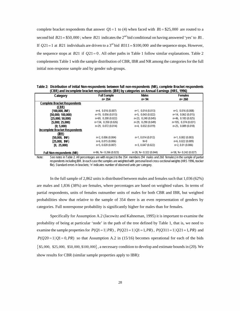
complements Table 1 with the sample distribution of CBR, IBR and NR among the categories for the full

initial non-response sample and by gender sub-groups.

Table 2: Distribution of initial Non-respondents between full non-respondents (NR), complete Bracket respondents (CBR) and incomplete bracket respondents (IBR) by categories on Annual Earnings (HRS, 1996)

Category Full Sample n= 354

Males n= 94

Females n= 260

Complete Bracket Respondents (CBR)

[100,000, INF) n=4, 0.016 (0.007) n=1, 0.014 (0.013) n=3, 0.016 (0.008) [50,000; 100,000) n=19, 0.056 (0.013) n=5, 0.043 (0.022) n=14, 0.062 (0.015) [25,000; 50,000) n=69, 0.200 (0.022) n=23, 0.240 (0.045) n=46, 0.183 (0.025) [5,000; 25,000) n=134, 0.350 (0.026) n=29, 0.290 (0.049) n=105, 0.374 (0.031)

[0; 5,000) n=29, 0.072 (0.014) n=4, 0.032 (0.019) n=25, 0.089 (0.018) Incomplete Bracket Respondents

(IBR)

[50,000, INF) n=2, 0.006 (0.004) n=1, 0.014 (0.012) n=1, 0.002 (0.003) [25,000, INF) n=6, 0.015 (0.006) N=0 n=6, 0.022 (0.009) [0, 25,000) n=5, 0.020 (0.007) n=3, 0.047 (0.022) n=2, 0.01 (0.006)

Full Non-respondents (NR)

n=86, %= 0.266 (0.023)

n=28, %= 0.322 (0.044)

n=58, %= 0.242 (0.027)

Note: See notes in Table 2. All percentages are with respect to the 354 members (94 males and 260 females) in the sample of partial respondents including IBR. In each case the samples are weighted with personal level cross-sectional weights (HRS 1996, tracker file). Standard errors in brackets; ‘n’ indicates number of observed units per category.

In the full sample of 2,862 units is distributed between males and females such that 1,036 (62%)

are males and 1,836 (38%) are females, where percentages are based on weighted values. In terms of

partial respondents, units of females outnumber units of males for both CBR and IBR, but weighted

probabilities show that relative to the sample of 354 there is an even representation of genders by

categories. Full nonresponse probability is significantly higher for males than for females.

Specifically for Assumption A.2 (Jacowitz and Kahneman, 1995) it is important to examine the

probability of being at particular ‘node’ in the path of the tree defined by Table 1, that is, we need to

examine the sample properties for ( 1 1| )P Q PR= , ( 21 1| 1 1, )P Q Q PR= = , ( 311 1| 21 1, )P Q Q PR= = and

( 20 1| 1 0, )P Q Q PR= = so that Assumption A.2 in (15/16) becomes operational for each of the bids

{ }$5,000, $25,000, $50,000, $100,000 , a necessary condition to develop and estimate bounds in (20). We

show results for CBR (similar sample properties apply to IBR):

29

Table 3: Sample Probabilities for different nodes in Table 1 using CBR to Annual Earnings, (HRS 1996) Probability at nodes defined by

Table 3 Full CBR Sample

n= 255 Males n= 62

Females n= 193

Conclusions with respect to HIGH or

LOW ANCHOR

( 1 1 | )P Q PR=

n=92/255

%= 0.283 (0.028)

n=29/62

%= 0.317 (0.059)

n=63/193

%= 0.217 (0.030)

Q1=1 B1 ($25,000) HIGH ANCHOR

( 21 1| 1 1, )P Q Q PR= =

n=19/92

%= 0.265 (0.048)

n=5/29

%= 0.192 (0.073)

¨ n=14/63

%= 0.299 (0.058)

Q21=1 B21 ($50,000)

HIGH ANCHOR

( 311 1| 21 1, )P Q Q PR= =

n=4/23 %= 0.217 (0.086)

n=1/6

%= 0.252 (0.178)

n=3/17

%= 0.206 (0.098)

Q311=1 B311 ($100,000)

HIGH ANCHOR

( 20 1| 1 0, )P Q Q PR= =

n=134/163 %= 829 (0.029)

n=29/33

%= 0.906 (0.051)

n=105/130

%= 0.807 (0.035)

Q20=1 B20 ($5,000)

LOW ANCHOR Note: See notes in Table 1 and 2. All percentages are with respect to the corresponding sub-groups. The indicator ‘n’ shows the total units

at each iQ given the number of units in the corresponding space. The probabilities are based on weighted averages. Bracketed numbers show standard errors.

Thus, from Table 3 and recalling the Jacowitz and Kahneman (1995) implications, we conclude

that the bids B1=$25,000, B21=$50,000 and B311=$100,000 act as ‘high anchors’ and the bid

B20=$5,000 acts as a ‘low anchor’. The information in Table 3 drives the characterization of (18) in

Appendix 2 (see Table A2.3). Finally, Table 4 examines the variable ‘earnings’ with two distinct sets of

information: weighted earnings using full respondents only (exogenous nonresponse assumption) and

weighted earnings when both non-respondents and partial respondents have had their missing values

imputed (constructed at sources, HRS, 1996 imputed variables files). The imputation method makes use

of partial information for those in the BR group taking this information as correct, i.e., imputed earnings

and bounds in (7) hold identical assumptions with respect to anchoring; in both cases the assumption is

that of no anchoring. This is not the case for bounds based on (13), (18) or (22) where different models of

anchoring relax the no anchoring assumption in (7).

Table 4: Sample statistics of gross annual earnings (standard errors in brackets)

Full Sample

Males

Females

Earnings, FR only

(n=2,508: male = 942, female = 1,566 ) Average (standard error)

Range $31,342 (566)

min=$0 max=$350,000 $36,202 (942)

min=$0 max=$300,000 $28,148 (695)

min=$0 max=$350,000Imputed earnings

(n=2,862: male = 1,036, female = 1,836 ) Average (standard error)

Range $30,867 (525)

min=$0 max=$350,000 $35,400 (876)

min=$0 max=$300,000 $28,040 (645)

min=$0 max=$350,000Note 1: Estimates are based on the weighted sample. The variable ‘earnings’ refers to ‘gross earnings’ and is based on an initial open-

ended question where individuals who declare to have worked over the last calendar year (i.e., 1995) are asked to declare the total gross amount of earnings received from such work. Amounts refer to nominal US dollars. The original variable draws from the publicly accessible HRS- 996 file named HR96J_H. The derived variable with the imputed amounts draws from the file named H96i_jh.

30

Table 4 suggests that males earn significantly more than females. Imputation of missing earnings

implies a slight drop in mean values for the full sample and for the sub-sample of males, but has weaker

effects on mean earnings for females. The standard errors do not differ much before and after imputation,

thus reflecting small noise induced from imputing non-respondents and partial respondents. This feature is

expected when imputation is performed in the support of the full response sample.

4.2 Specification Section 2 provides the general expression for bounds that allow for partial information when

initial respondents are routed to an unfolding design with J possible conditional bids resulting in 2J

categories for CBR and 2J d− categories for IBR (see Section 2.3). Table 1 shows that for the specific case

under consideration J is at most 3; in the case of CBR the number of resulting categories are 21 2+ = 5

where the ‘1’ accounts for the special case of an asymmetric design at 3B . On the other hand, IBR define

3 distinct categories. The partition { }[0, 20),[ 20, 1),[ 1, 21),[ 21, 311),[ 311, )B B B B B B B BY ∞= defines the

support for CBR, whereas IBR define an alternative partition with overlapping categories:

{ }[0, 21),[ 1, ),[ 21, )B B BY ∞ ∞= . The two sub-groups of partial respondents have bids in common and this

helps to join the sample information from the two groups to estimate identification regions on

( | )F y gender for different y Bτ< . Appendix 2 characterizes (7), (13), (18) and (22) for the particular

case when the unfolding design follows the example as in Table 1.

4.3 Bounds, Bracket Respondents and anchoring First we use bracket respondents to validate the properties of imputed earning. The HRS

imputation procedure assumes no anchoring effects. This is in fact the same assumption characterizing

bounds in (7). Comparing estimates based on imputed values to estimate of bounds in (7) is a test of the

assumptions (other than no anchoring) underlying the imputation process. Figure 1 in Table 5 plots the

distribution using the 268 bracket respondent’s imputed earnings. Figure 2 plots the interval identified

using the original information provided by the 268 bracket respondents.16 Figure 3 compares Figure 1 to

Figure 2 with the corresponding 95% confidence intervals (dashed lines in each original figure). Imputing

values results in a continuous earning’s variable and therefore in a continuous distribution function

(Figure 1); in this case the median is located between $19,200 -- $23,900 with 95% confidence. Using the

original unfolding bracket’s information respondents identify an earning’s category so that information is

discrete in nature and the results are bounds shaped as step functions (Figure 2): in this case the median is

16 Bounds in Figure 2 are based on estimates from (27) thus inverting the estimate of the distribution function from (7). The upper

bound in (7) becomes the lower bound for quantiles in (27) and the lower bound in (7) becomes the upper bound for quantiles

in (27).

31

located between $4,800 – $25,000; this region of identification is also based on a 95% confidence

interval, but it includes uncertainty from both sampling error and partial (as opposed to exact)

information. Thus, in the case of the median, the result is a width that is 77% wider than that in Figure 1.

The estimated upper and lower bounds in Figure 2 meet exactly at $25,000 and $50,000; the gap at $5,000

and $100,000 reflects the effect of asymmetric overlapping categories from IBR. In the absence of this

subgroup of partial respondents upper and lower bounds would meet exactly at all bids in the design.

Finally, and ‘holding the no anchoring assumption’, Figure 3 demonstrates that the imputed variable

cannot be rejected because the 95% confidence region identified using imputation is nested by that

identified with the step function interval (also with 95% confidence).

Table 5: Bracket response information, comparing imputed values and bounding intervals (A0)

0 0.1 0.2 0.3 0.4 0.5 0.6 0.7 0.8 0.9 16

7

8

9

10

11

12

Quantiles of the distribution

Earn

ings

in U

SA$,

nat

ural

logs

Figure 1: Imputed values, Partial information

____ _ _ _

95%Estimates Confidence

0 0.1 0.2 0.3 0.4 0.5 0.6 0.7 0.8 0.9 16

7

8

9

10

11

12Figure 2: Bracket Respondents, No Anchoring (A0)


Earn

ings

in U

SA$,

nat

ural

logs

____ _ _ _

95%Estimates Confidence

0 0.1 0.2 0.3 0.4 0.5 0.6 0.7 0.8 0.9 16

7

8

9

10

11

12


Earn

ings

in U

SA$,

nat

ural

logs

Figure 3: Comparing Confidence Intervals, F1 - F2

95% , 1 95% , 2

_ _ _ ____ ____CI F CI F

Note: The horizontal range has been artificially trimmed between $500 and $160,000 for a clearer illustration. Below and above these values the plots do not provide further information.

Figures 1 to 3 ignore possible anchoring effects. Table 6 compares the effect of three different

anchoring assumptions (A1 to A3) against the no anchoring Assumption A0.17 Compared to Figure 4

(A0), all other figures clearly show that relaxing the assumption of no anchoring leads to a loss in the

power of the identification region. The loss differs between anchoring assumptions and according to

quantiles. With 95% confidence, Assumption A1 identifies the median between $4,800 and the maximum

value in the range of earnings ($350,000). Also with 95% confidence Assumption A2 identifies the same

quantile between $4,800 and $25,000 whereas Assumption A3 identifies the median between $0 and

$25,000. Figure 5 show anchoring effects based on Hurd et al. (1998) where the median assumption

widens the identification region for all the quantiles in the distribution. Assumption A2 implies the

findings in Jacowitz and Kahneman where ‘high’ and ‘low’ perceived anchors affect the tails of the

distribution: accounting for these effects leads to bounding intervals with thicker tails as reflected in

Figure 6. Assumption 3 defines no anchoring at the first bid and this is reflected with a point estimate at

$25,000 that is identical to that in Figure 4 (A0): since anchoring based on A3 implies answers that are

17 Figure 2 is identical to Figure 4. It is included in Table 6 for better visual comparison.

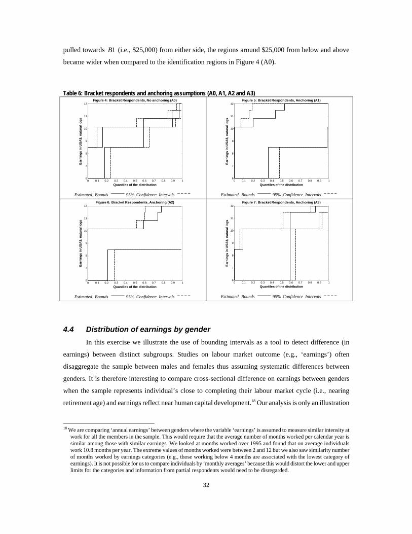
32

pulled towards 1B (i.e., $25,000) from either side, the regions around $25,000 from below and above

became wider when compared to the identification regions in Figure 4 (A0).

Table 6: Bracket respondents and anchoring assumptions (A0, A1, A2 and A3)

0 0.1 0.2 0.3 0.4 0.5 0.6 0.7 0.8 0.9 16

7

8

9

10

11

12


Earn

ings

in U

SA$,

nat

ural

logs

Figure 4: Bracket Respondents, No anchoring (A0)

______ _ _ _ _

95%Estimated Bounds Confidence Intervals

0 0.1 0.2 0.3 0.4 0.5 0.6 0.7 0.8 0.9 16

7

8

9

10

11

12


Earn

ings

in U

SA$,

nat

ural

logs

Figure 5: Bracket Respondents, Anchoring (A1)

______ _ _ _ _


0 0.1 0.2 0.3 0.4 0.5 0.6 0.7 0.8 0.9 16

7

8

9

10

11

12


Earn

ings

in U

SA$,

nat

ural

logs


______ _ _ _ _


0 0.1 0.2 0.3 0.4 0.5 0.6 0.7 0.8 0.9 16

7

8

9

10

11

12


Earn

ings

in U

SA$,

nat

ural

logs


______ _ _ _ _


4.4 Distribution of earnings by gender In this exercise we illustrate the use of bounding intervals as a tool to detect difference (in

earnings) between distinct subgroups. Studies on labour market outcome (e.g., ‘earnings’) often

disaggregate the sample between males and females thus assuming systematic differences between

genders. It is therefore interesting to compare cross-sectional difference on earnings between genders

when the sample represents individual’s close to completing their labour market cycle (i.e., nearing

retirement age) and earnings reflect near human capital development.18 Our analysis is only an illustration

18 We are comparing ‘annual earnings’ between genders where the variable ‘earnings’ is assumed to measure similar intensity at

work for all the members in the sample. This would require that the average number of months worked per calendar year is similar among those with similar earnings. We looked at months worked over 1995 and found that on average individuals work 10.8 months per year. The extreme values of months worked were between 2 and 12 but we also saw similarity number of months worked by earnings categories (e.g., those working below 4 months are associated with the lowest category of earnings). It is not possible for us to compare individuals by ‘monthly averages’ because this would distort the lower and upper limits for the categories and information from partial respondents would need to be disregarded.

33

of Section 2 with no policy implication since we are not conditioning on variables that might imply policy

analysis.

Our concern is to perform the comparison between genders taking into account that 12% in the

representative sample do not declare annual earnings, although they have declared to have worked for pay

during the corresponding calendar year. Ignoring these 12% may bias our inference if nonresponse is not

random with respect to earnings. Allowing for imputed variables implies the use of the assumptions

underlying the imputation procedure (e.g., ignoring possible anchoring effects from bracket respondents)

that may also bias our inference: Figure 8 shows the result of comparing 95% confidence bands on the

quantiles of earnings between genders and using the complete sample with missing values imputed. 19

Alternatively, we estimate identification regions on the quantiles of earnings that allow for any type of

non-random nonresponse at the expense of this nonresponse contributing towards total uncertainty.

Figures 9 to 13 do this with various assumptions on how to deal with bracket response information; in

these figures the vertical distance between bounds is the sum of nonresponse error and sampling error also

with 95% confidence. All figures in Table 7 help to test for earnings difference between the two genders

by comparing the location of identification regions between the two subgroups. Table 8 complements

Figures 8 – 13 with a formal test on a selection of quantiles. All figures in Table 7 are based on estimating

all versions of (23) and inverting these estimates to obtained (27).

Figure 8 shows that once the missing values are imputed the identification region for male is

always above that identified for females, with 95% confidence. Thus, imputation would imply rejecting

the null of earnings equality between genders in favour of males receiving significantly higher earnings

than females at any level of earning. Figure 9 relaxes all assumptions implied by imputation to allow for

any type of nonresponse error thus increasing total uncertainty when estimating the identification regions.

At the same time, Figure 9 is based on expression (2) so that information from partial respondents is

ignored. Thus, Figure 9 implies a loss in the power of the test when compared to Figure 8. This is clear

since overlapping regions in Figure 9 imply that we cannot reject the null of earning equality between

genders at any level of earnings. Figure 10 improves the power of the test by including information

provided by bracket respondents but ignoring possible anchoring effects (A0). In Figure 10 overlapping

of the 95% confidence intervals is only visible a α -quantiles below 0.3 and above 0.85, but the null of

earning’s equality between genders is rejected for middle earning’s quantiles. Figures 11 to 13 apply (13),

(18) and (22) to relax the assumption of no anchoring implied by Figure 10. The results vary between the

19 Pointwise estimate with imputation, or estimates of bounds are always nested by their 95% confidence intervals. Figures in

Table 7 reflect these 95% confidence intervals for ease of illustration. For example, Figure 9 shows the median for males bounded between $26,200 and $36,900 with 95% confidence, but the actual pointwise estimated upper and lower bounds locate the median between $29,900 and $34,600; this latter interval reflects only uncertainty as result of item nonresponse. We choose to illustrate upper and lower bounds using 95% confidence intervals because the use of 4 (rather than 8 curves) in one plot clarifies the comparison between genders. Table 8 complements these figures showing point estimates for a selection of quantiles.

34

three figures but all have in common a loss in the power of the test as total uncertainty in estimation

increases. Table 8 complements Figures 8 – 13 with a formal test that covers a selection of quantiles.

Table 7: Bounding intervals with and without bracket respondents and no anchoring effects

0 0.1 0.2 0.3 0.4 0.5 0.6 0.7 0.8 0.9 16

7

8

9

10

11

12


Earn

ings

in U

SA$,

nat

ural

logs

Figure 8: Earnings with Imputed missing values

______ _ _ _ _

95% :Confidence Intervals Females Males

0 0.1 0.2 0.3 0.4 0.5 0.6 0.7 0.8 0.9 16

7

8

9

10

11

12

Quantile of the distribution

Earn

ings

in U

SA$,

nat

ural

logs

Figure 9: Bounds without Bracket respondents

______ _ _ _ _


0 0.1 0.2 0.3 0.4 0.5 0.6 0.7 0.8 0.9 16

7

8

9

10

11

12


Earn

ings

in U

SA$,

nat

ural

logs

Figure 10: Bounds with FR, BR, NR: No Anchoring (A0)

______ _ _ _ _


0 0.1 0.2 0.3 0.4 0.5 0.6 0.7 0.8 0.9 16

7

8

9

10

11

12


Earn

ings

in U

SA$,

nat

ural

logs

Figure 11: Bounds with FR, BR, NR: Anchoring (A1)

______ _ _ _ _


0 0.1 0.2 0.3 0.4 0.5 0.6 0.7 0.8 0.9 16

7

8

9

10

11

12


Earn

ings

in U

SA$,

nat

ural

logs


______ _ _ _ _


0 0.1 0.2 0.3 0.4 0.5 0.6 0.7 0.8 0.9 16

7

8

9

10

11

12


Earn

ings

in U

SA$,

nat

ural

logs


______ _ _ _ _


35

Table 8: Testing for Quantile difference between genders. Amounts refer to annual earnings in USA Dollars (HRS, 1996)

Quantile Estimates Male Upper bound

(standard error)

Quantile Estimate Female

Lower bound (standard error)

Quantile Difference: Male (Lower bond) – Female (Upper

bound)

T-statistic ( bootstrap

critical values)

IMPUTATION (FIG. 8)1 25th Percentile 40th Percentile 50th Percentile 60th Percentile 75th Percentile 90th Percentile

14,700 (1,285) 25,000 (786) 29,900 (764)

35,600 (1,219) 47,500 (1,146) 61,000 (2,199)

10,800 (800) 17,900 (522) 21,900 (765) 25,900 (879)

35,600 (1,027) 53,900 (1,307)

3,900 7,100 8,000 9,700 11,900 7,100

2.6 (2.8) 7.4 (2.2) 7.5 (1.8) 6.5 (1.9) 7.7 (2.1) 2.8 (2.7)

BOUNDS, NO BRACKETS (FIG. 9) 25th Percentile 40th Percentile 50th Percentile 60th Percentile 75th Percentile 90th Percentile

11,900 (1,035) 22,800 (1,322) 29,900 (1,104) 34,600 (1,250) 48,000 (1,528) 65,500 (2,350)

12,750 (503) 20,500 (946) 25,900 (815)

32,000 (1,177) 49,700 (1,386) 350,000 (0,00)

-850 2,300 4,000 2,600 -1,760

-285,500

-0.8 (-2.7) 1.4 (2.0) 2.9 (0.7) 1.5 (1.8)

-0.9 (-2.3) -121.5 (-2.3)

BOUNDS, and BRACKETS with A0 (FIG. 10) 25th Percentile 40th Percentile 50th Percentile 60th Percentile 75th Percentile 90th Percentile

13,700 (1,180) 25,000 (751) 29,900 (985)

35,600 (1,235) 48,000 (1,414) 64,500 (2,337)

11,900 (537) 19,500 (581) 25,000 (178) 27,900 (946)

39,400 (1,080) 62,000 (2,784)

1,800 5,500 5,000 7,800 8,600 2,500

1.4 (1.6) 5.8 (1.1) 4.9 (1.1) 5.0 (1.5) 4.8 (1.5) 0.7 (1.5)

BOUNDS, and BRACKETS with A1 (FIG. 11) 25th Percentile 40th Percentile 50th Percentile 60th Percentile 75th Percentile 90th Percentile

11,900 (1,032) 22,800 (1,292) 29,900 (1,104) 34,600 (1,250) 47,900 (1,528) 64,500 (2,350)

12,800 (503) 20,500 (946) 25,000 (255) 29,900 (872)

44,500 (2,535) 98,000 (89,461)

-850 2,300 5,000 4,700 3,500

-33,500

-0.7 (-2.1) 1.4 (2.0) 4.3 (0.0) 3.1 (2.0) 1.2 (1.3)

-0.4 (-2.9) BOUNDS, and BRACKETS with A2 (FIG. 12)

25th Percentile 40th Percentile 50th Percentile 60th Percentile 75th Percentile 90th Percentile

11,900 (1,015) 22,800 (1,322) 29,900 (1,104) 34,600 (1,250) 48,000 (1,530) 64,500 (2,350)

12,800 (503) 20,500 (946) 25,000 (240) 27,900 (947)

39,400 (1,107) 69,000 (6,985)

-850 2,300 5,000 6,700 8,600 -4,500

-0.8 (-2.7) 1.4 (2.0) 4.5 (2.0) 4.3 (1.9) 4.5 (0.9)

-0.6 (-3.2) BOUNDS, and BRACKETS with A3 (FIG. 13)

25th Percentile 40th Percentile 50th Percentile 60th Percentile 75th Percentile 90th Percentile

13,700 (1,180) 25,000 (751) 29,900 (894)

35,600 (1,235) 48,000 (1,414) 64,500 (2,317)

12,800 (482) 19,500 (680) 25,000 (83)

27,900 (946) 39,400 (1,100) 74,200 (6,800)

950

5,500 5,000 7,700 8,600 -9,700

0.7 (2.3) 5.4 (0.8) 5.0 (0.1) 5.0 (1.5) 4.8 (1.5)

-1.4 (-3.3) 1 In the case of imputed values the point estimates are exactly identified. Thus, the test is based on the quantiles difference (males -

females) normalized by the corresponding standard error. For all other rows in Table 8 the test is based on (male’s lower bound – female’s upper bound) also normalized by the corresponding standard error.

2 The 1000 bootstrap estimates of the difference are used to find the empirical distribution for the t-statistic centered on the original estimate of the difference. This provides the bootstrap critical values based on the upper 2.5 percentile of the empirical t-distribution using an equal tail test. Therefore, the null of equality is rejected at a 0.05 level when the estimate of the t-statistic is greater or equal than the bootstrap critical value (in brackets).

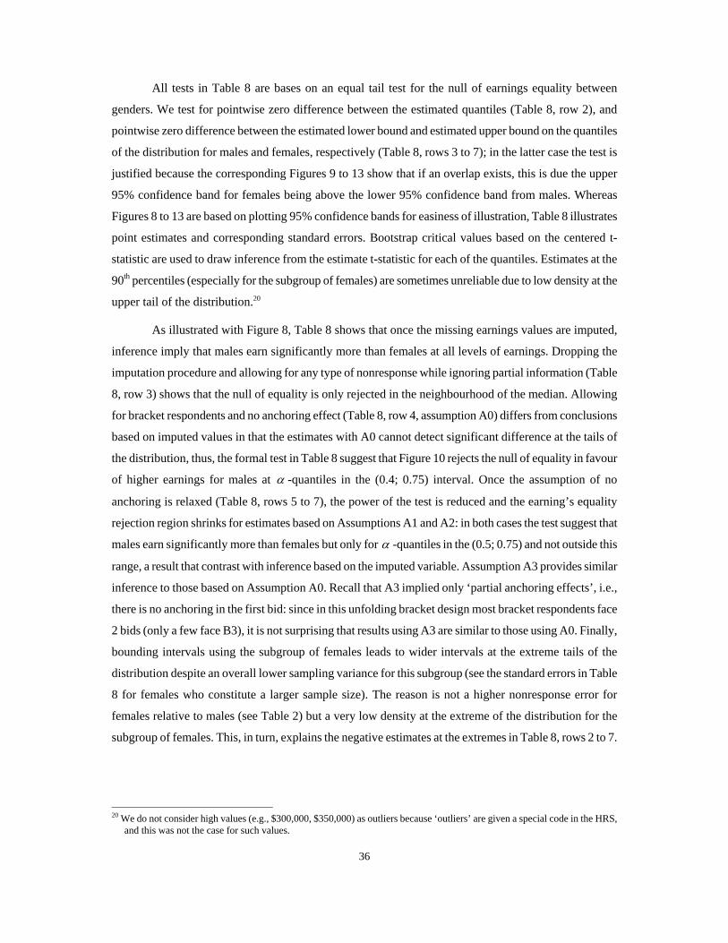
36

All tests in Table 8 are bases on an equal tail test for the null of earnings equality between

genders. We test for pointwise zero difference between the estimated quantiles (Table 8, row 2), and

pointwise zero difference between the estimated lower bound and estimated upper bound on the quantiles

of the distribution for males and females, respectively (Table 8, rows 3 to 7); in the latter case the test is

justified because the corresponding Figures 9 to 13 show that if an overlap exists, this is due the upper

95% confidence band for females being above the lower 95% confidence band from males. Whereas

Figures 8 to 13 are based on plotting 95% confidence bands for easiness of illustration, Table 8 illustrates

point estimates and corresponding standard errors. Bootstrap critical values based on the centered t-

statistic are used to draw inference from the estimate t-statistic for each of the quantiles. Estimates at the

90th percentiles (especially for the subgroup of females) are sometimes unreliable due to low density at the

upper tail of the distribution.20

As illustrated with Figure 8, Table 8 shows that once the missing earnings values are imputed,

inference imply that males earn significantly more than females at all levels of earnings. Dropping the

imputation procedure and allowing for any type of nonresponse while ignoring partial information (Table

8, row 3) shows that the null of equality is only rejected in the neighbourhood of the median. Allowing

for bracket respondents and no anchoring effect (Table 8, row 4, assumption A0) differs from conclusions

based on imputed values in that the estimates with A0 cannot detect significant difference at the tails of

the distribution, thus, the formal test in Table 8 suggest that Figure 10 rejects the null of equality in favour

of higher earnings for males at α -quantiles in the (0.4; 0.75) interval. Once the assumption of no

anchoring is relaxed (Table 8, rows 5 to 7), the power of the test is reduced and the earning’s equality

rejection region shrinks for estimates based on Assumptions A1 and A2: in both cases the test suggest that

males earn significantly more than females but only for α -quantiles in the (0.5; 0.75) and not outside this

range, a result that contrast with inference based on the imputed variable. Assumption A3 provides similar

inference to those based on Assumption A0. Recall that A3 implied only ‘partial anchoring effects’, i.e.,

there is no anchoring in the first bid: since in this unfolding bracket design most bracket respondents face

2 bids (only a few face B3), it is not surprising that results using A3 are similar to those using A0. Finally,

bounding intervals using the subgroup of females leads to wider intervals at the extreme tails of the

distribution despite an overall lower sampling variance for this subgroup (see the standard errors in Table

8 for females who constitute a larger sample size). The reason is not a higher nonresponse error for

females relative to males (see Table 2) but a very low density at the extreme of the distribution for the

subgroup of females. This, in turn, explains the negative estimates at the extremes in Table 8, rows 2 to 7.

20 We do not consider high values (e.g., $300,000, $350,000) as outliers because ‘outliers’ are given a special code in the HRS,

and this was not the case for such values.

37

5 Conclusions Manski’s approach to deal with item nonresponse avoids the assumptions usually associated with

parametric and semi-parametric methods. On the other hand, it identifies the unknown parameters up to an

upper and lower bound only. In this paper, these bounds are extended to take account of the information

contained in follow up categorical questions to initial non-respondents. Such questions are included in

many current household surveys (e.g., the Health and Retirement Study and related panels, or the

SHARE, the counterpart of the HRS in Europe). Several studies have shown that responses to such

questions can be subject to response errors due to anchoring effects. Some exiting studies model this

response error with a parametric set up. We have extended the Manski’s bounds to allow for anchoring in

a nonparametric way, starting from various nonparametric anchoring assumptions inspired by the existing

parametric models. Thus, our bounds simultaneously allow for any type of selective nonresponse and

various forms of anchoring.

Using the variables earnings (wages and salary) of the household representative taken from the

1996 wave of the Household and Retirement Study, the empirical section shows estimates of Manski’s

basic worst case bounds that do not use the bracket respondents information and compares these with

estimates of the new bounds. For the variable considered, the initial (weighted) nonresponse rate is 12%.

Most of the initial non-respondents answer unfolding bracket questions, and the percentage of (weighted)

full nonresponse rate drops to 3%. Incorporating information provided by bracket respondents tightens the

bounds. Allowing for anchoring effects reduces the gains in information but still leads to estimated

bounds that are substantially more informative than the bounds that do not use bracket information. This

is illustrated by using the bounds to test for equality of quantiles between genders. Adding the information

provided by bracket respondents improves the power of the tests, and leads to rejecting the null more

often. How much the power of the tests increases depends on whether and how anchoring is allowed for.

Manski’s bounds are an elegant, intuitively plausible and extremely flexible way to allow for

selective nonresponse. Their flexibility is at the same time their main weakness: the bounds are often so

wide that they do not provide enough information for the economic issue under consideration. This paper

shows that additional information on bracket responses by initial non-respondents can be useful to make

the bounds more informative. This is still true if anchoring is allowed for, though to a lesser extent.

Furthermore, we have used the bounds to validate the imputation procedure used to impute missing

earnings values for the HRS publicly released data. Missing values are imputed using information from

bracket respondents and assuming no anchoring effects. We show that using imputed values to make

inference on earnings equality between genders leads to different conclusions than those implied by the

bounding interval: with this latter earning’s differentials between genders is often rejected at the upper

and lower tail of the distribution. In the light of the findings in Hurd et al. (1998) where anchoring effects

38

are detected, the use of bounds might be called for instead of an imputed variable that ignores possible

anchoring effects.

The bounds are estimated allowing for different types of anchoring each generalizing a different

parametric model in the exiting literature. The paper does not analyse which model of anchoring is most

appropriate: this is not a relevant question for this framework. With the current data, however, selective

nonresponse and anchoring interact, and it is hard to say something about anchoring without making

strong assumptions about the nature of nonresponse. For an analysis of anchoring itself, therefore,

experimental data where all respondents get bids that vary randomly across the sample, such as in the

experimental HRS module used by Hurd et al. (1998), is more appropriate. With more knowledge about

the nature of the anchoring process, the analysis here could be refined.

References Borgers, N and J. Hox, (2001), Item nonresponse in questionnaire research with children, Journal of Official

Statistics, 17,2, 321-335 Cameron, T. and J. Quiggin, (1994), Estimation using contingent valuation data from a dichotomous choice with

follow-up questionnaire, Journal of Environmental Economics and Management, 27, 218-234 Ginther, D., (2000), Alternative estimates of the effect of schooling on earnings, Review of Economics and Statistics,

82,1, 102 - 116 Green, D., K. Jacowitz, D. Kahneman and D. McFadden (1998), Referendum contingent valuation, anchoring, and

willingness to pay for public goods, Resource and Energy Economics, 20, 85-116 Hädler, W., (1990), Applied nonparametric regression, Econometric Society Monographs, 19, Cambridge University

Press, Cambridge Herriges, J. and C. Shogren, (1996), Starting point bias in dichotomous choice valuation with follow-up questioning,

Journal of Environmental Economics and Management, 30, 112-131 Horowitz, J. and C. Manski, (1995), Identification and robustness with contaminated and corrupted data,

Econometrica, 63,2, 281-302 Horowitz, J. and C. Manski, (1998), Censoring of outcomes and regressors due to survey nonresponse: identification

and estimation using weights and imputations, Journal of Econometrics, 84, 37-58 Hurd, M., D. McFadden, H. Chand, L.Gan, A. Merrill and M. Roberts, (1998), Consumption and savings balances of

the elderly: Experimental evidence on survey response bias, in D. Wise (ed.), Frontiers in the Economics of Aging, University of Chicago Press, Chicago, 353-387

Jacowitz, K. and D. Kahneman (1995), Measures of anchoring in estimation tasks, Personality and Social Psychology Bulletin, 21, 1161- 1166

Juster, T. and J. Smith (1997), Improving the quality of economic data: Lessons from the HRS and AHEAD, Journal of the American Statistical Association, 92, 1268-1278

Manski, C., (1989), Anatomy of the selection problem, Journal of Human Resources, 24, 343-360 Manski, C., (1990), Non-parametric bounds on treatment effects, American Economic Review, Papers &

Proceedings, 80, 319-323 Manski, C., (1994), The selection problem in ‘Advances in Econometrics’, C. Sims (ed.), Cambridge University

Press, 143-170 Manski, C., (1995), Identification problems in the social sciences, Harvard University Press Manski, C., (1997), Monotone treatment response, Econometrica, 68, 1311-1334 Manski, C., and J. Pepper, (2000), Monotone instrumental variables with an application to the returns to schooling,

Econometrica, 68, 997-1010

39

Mason, R., V. Lesser, and M. Traugott, Effect of item nonresponse on nonresponse error and inference, In Groves, R., D. Dillman, J. Eltinge and R. Little (eds.), Survey Nonresponse, Wiley, New York, 2002.

O’Connor, R. M. Johansson and P. Johansson (1999), Stated preferences, real behaviour and anchoring: some empirical evidence, Environmental and Resource Economics, 13, 235-248.

Pepper, J. (2000), The inter-generational transmission of welfare receipts: a non-parametric bounds analysis, The Review of Economics and Statistics, 82, 472-488

Pepper, J. (2003), Using experiments to evaluate performance standards, what do welfare to work demonstrations reveal to welfare reformers?, Journal of Human Resources, 38,4, 860-880

Rabin, M. (1998), Psychology and Economics, Journal of Economic Literature, 11-46. Switzer, F. and J. Sniezek, (1991), Judgement processes in motivation: anchoring and judgement effects on

judgement and behaviour, Organizational Behaviour and Human Decision Process, Vol. 49, 208-229 Tourangeau, R., L. Rips and K. Rasinski (2000), The psychology of survey response, New York and Cambridge

University Press Tversky, A. and D. Kahneman, (1974), Judgement under uncertainty: Heuristics and biases, Science, 185, 1124-1131 Vazquez-Alvarez, R., (2006), Anchoring effects and covariates nonresponse, Department of Economics DP series,

University of St.Gallen Wilson, T. D., C. Houston, K. Etling, and N. Brekke (1996), A new look at anchoring effects: basic anchoring and

its antecedents, Journal of Experimental Psychology,. 135, 387-402

Appendix 1: Deriving bounds (13) on ( | , )F y x BR with Assumption A.1

Bounds in (13) result from applying conditions in (12) to derive upper and lower bounds on

( | , )P Y B x BRτ< . Conditions in (12) imply the following:

:

( ) 1 & 0(12. ), (12. ) ( | , )

( ) 1 & 1(12. ), (12. ) ( | , )

( ) ( ) (

Let B be the bid that follows B from Q and Q

i Q Q B Ba e apply to bound P Y B x BR

ii Q Q B Bc e apply to bound P Y B x BR

i and ii define upper and lower bounds on P Y B

τ τ τ τ

τ τ τ τ

τ

τ τ τ τ

τ

− −

− −

− −

= = ⇒ >⇒ <

= = ⇒ >

⇒ ≥

⇒ < | , ),

( ) 0 & 0(12. ), (12. ) ( | , )

( ) 1 & 0(12. ), (12. ) ( | , )

( ) ( )

x BR fora bids B above some bid B implied by Q where Q leads to B

iii Q Q B Bb e apply to bound P Y B x BR

vi Q Q B Bd e apply to bound P Y B x BR

iii and vi define u

τ

τ τ τ τ τ

τ τ τ τ

τ

τ τ τ τ

τ

− −

− −

− −

= = ⇒ <⇒ <

= = ⇒ <⇒ ≥

⇒ ( | , ),

pper and lower bounds on P Y B x BR fora bids B below some bid B implied by Q where Q leads to B

τ

τ τ τ τ τ− −

<

(A1.1)

Apply the rubric in (A1.1) to both ( | , )P Y B x BRτ< and ( | , )P Y B x BRτ≥ , where the following

interpretation applies to link reported fractions and unknown conditional distributions:

40

( ) ( | , ) ( | , , 1) ( 1| , )( | , , 0) ( 0 | , )

( ) ( | , ) ( | , , 1) ( 1| , )( | , , 0) ( 0 | , )

a P Y B x BR P Y B x BR Q P Q x BRP Y B x BR Q P Q x BR

and

b P Y B x BR P Y B x BR Q P Q x BRP Y B x BR Q P Q x BR

τ τ τ τ

τ τ τ

τ τ τ τ

τ τ τ

< = < = =+ < = =

≥ = ≥ = =+ ≥ = =

(A1.2)

Once the position of Bτ is decided relative to B τ− , i.e., B Bτ τ−< or B Bτ τ−> ,21 deriving the two

bounds in (13) is rooted in applying the two sets of results in (A1.1) to (A1.2). We proceed to show the

application of ( )i and ( )ii to (A1.2):

( )(12. )

, (12. ) (12. ) ( | , ) :

( ) ( | , ) ( | , , 0) ( 0 | , )( | , , 1) ( 1| , )( | , ) ( 0 | , )

2 ( 0 | , , 1) ( 1| , )applying e

a

For B B a and e bounds P Y B x BR from above

a P Y B x BR P Y B x BR Q P Q x BRP Y B x BR Q P Q x BRP Y B x BR P Q x BR

P Q x BR Q P Q x BR

τ τ τ

τ τ τ τ

τ τ τ

τ τ

τ τ τ

−

−

> <

< = < = =+ < = =

≤ < =

+ = = = ( )

[ ]

(12. )

. , 2 ( 0 | , , 1)

( | , ) min 1, 2 ( 0 | , , 1)

, (12. ) (12. ) ( | , ) :

( ) ( | , ) ( | , , 0) ( 0 | , )( | , ,

pplying a

i e P Q x BR Q

Upper Bound P Y B x BR P Q x BR Q

For B B c and e bounds P Y B x BR from bellow

b P Y B x BR P Y B x BR Q P Q x BRP Y B x BR Q

τ τ

τ τ τ

τ τ τ

τ τ τ τ

τ τ

−

−

−

≤ = =

⇒ < ≤ = =

> ≥

≥ = ≥ = =+ ≥ =

( )( )

[ ]

(12. )

(12. )

1) ( 1| , )( | , ) ( 0 | , )

2 ( 1| , , 1) ( 1| , ). , 2 ( 1| , , 1)

( | , ) min 1, 2 ( 1| , , 1)

1 ( | , ) 1 min 1, 2 ( 1| , ,

applying e

applying c

P Q x BRP Y B x BR P Q x BR

P Q x BR Q P Q x BRi e P Q x BR Q

P Y B x BR P Q x BR Q

P Y B x BR P Q x BR Q

τ

τ τ

τ τ τ

τ τ

τ τ τ

τ τ τ

−

−

−

−

=

≤ ≥ =

+ = = =

≤ = =

⇒ ≥ ≤ = =

⇒ − ≥ ≥ − =[ ]

[ ]

1)

( | , ) max 0,1 2 ( 1| , , 1)Lower Bound P Y B x BR P Q x BR Qτ τ τ−

=

⇒ < ≥ − = =

(A1.3)

The result in (A1.3) is shown in Section 2 with (13.b). Deriving bounds in (13.a) follow in the

same manner, but using ( )iii and ( )iv in (A1.1) in (A1.2) instead of ( )i and ( )ii . Notice that the result in

21 For example, Bτ =$5,000 is such that B Bτ τ−< if compared to B τ− =$25,000, whereas Bτ =$50,000 is such that B Bτ τ−> if

compared to B τ− =$25,000.

41

(A1.3) is not trivial when compared to (12.a), i.e., Assumption A1 leads to a bound on the conditional

distribution ( | , , 1)P Y B x BR Qτ τ−< = , and we use this together with (12.e) to derive an upper bound on

( | , )P Y B x BRτ< given in (A1.3).

Appendix 2: Characterizing bounds (7), (13), (18) and (22) Section 4.1, Table 1 defines an unfolding bracket design such that respondents can face as many

as 3 bids. The unfolding design is asymmetric in the sense that not all respondents face the same number

of bids. Only those follow the design towards the higher conditional bids face at most 3 bids. Otherwise,

individuals face at most 2 bids. With this, those who become CBR are able to classify the otherwise

undisclosed amount in one out of five categories: [0, 20)B , [ 20, 1)B B ,[ 1, 21)B B ,[ 21, 311)B B and

[ 311, )B ∞ ; empirically, all these categories are nonempty. The IBR subgroup defines three categories,

[0, 1)B , [ 1, )B ∞ , and [ 21, )B ∞ , and all three are empirically nonempty. Bonds on ( | , )F y x BR are

characterized according to these categories.

Characterising Bounds in (7)

Table A2.1: Characterizing ( | , )F y x BR for bounds in (7): Assumption A0 Contribution to Lower Bound on

( | , )F y x BR weighted by ( | , )P R x BR

Contribution to Upper Bound on ( | , )F y x BR weighted by

( | , )P R x BR Complete Bracket Respondents

where ( | , ) ( | , )P R x BR P CBR x BR=

[0, 20)B 0 ( 20 0 | , )P Q x CBR= [ 20, 1)B B ( 20 0 | , )P Q x CBR= ( 1& 20 0 | , )P Q Q x CBR= [ 1, 21)B B ( 1& 20 0 | , )P Q Q x CBR= ( 21& 1& 20 0 | , )P Q Q Q x CBR=

[ 21, 311)B B ( 21& 1& 20 0 | , )P Q Q Q x CBR= ( 311& ... & 20 0 | , )P Q Q x CBR= [ 311, )B ∞ ( 311& ... & 20 0 | , )P Q Q x CBR= 1

Complete Bracket Respondents where

( | , ) ( | , )P R x BR P IBR x BR=

[0, 1)B 0 ( 1 0 | , )P Q x IBR= [ 1, )B ∞ ( 1 0 | , )P Q x IBR= 1

[ 21, )B ∞ ( 1& 21 0 | , )P Q Q x IBR= 1

42


A pre-requisite is to define the relation between Bτ & B τ− for each bid in 1[ , )B Bτ τ− . For

example, Table 1 shows that to be in [0, 20)B , 20B is determined because 1 0Q = to 1B and 20 0Q = .

Thus, relative to 1 ( )B B τ−= , 20 1B B< and (13.a) applies to 20B for bounds on 1[ , ) [0, 20)B B Bτ τ− = ; it

implies that { } { }max[0,1 2 ( 20 1 | , , 1 0)], min[1, 2 ( 20 0 | , , 1 0)]( ), ( ) P Q x BR Q P Q x BR Ql B u Bτ τ − = = = == whereas

{ } { }1 1 0,0( ), ( )l B u Bτ τ− − = . From (13), [ ]{ }1, 0, max 0,1 2 ( 20 1 | ...)min P QLτ τ− − == so that 1, 0Lτ τ− = , while

[ ]{ }1, 0, min 1, 2 ( 20 0 | , , 0)max P Q x BR QUτ τ τ− −= == so that [ ]1, min 1, 2 ( 20 0 | , , 0)P Q x BR QUτ τ τ− −= == . Similar

arguments determine all entries in Table A2.2 below:


( | , )F y x BR weighted by ( | , )P R x BR Contribution to Upper Bound on

( | , )F y x BR weighted by ( | , )P R x BR Complete Bracket

Respondents where ( | , ) ( | , )P R x BR P CBR x BR=

[0, 20)B 0 { }0

maxmin[1, 2 ( 20 0 | , , 1 0)]P Q x CBR Q= =

[ 20, 1)B B { }max[0,1 2 ( 20 1 | , , 1 0)]min

max[0,1 2 ( 1 1 | , )]P Q x CBR Q

P Q x CBR− = =

− = { }min[1, 2 ( 20 0 | , , 1 0)]

maxmin[1, 2 ( 1 0 | , )]

P Q x CBR QP Q x CBR

= ==

[ 1, 21)B B { }max[0,1 2 ( 1 1 | , )]min

max[0,1 2 ( 21 1 | , , 1 1)]P Q x CBR

P Q x CBR Q− =

− = = { }min[1, 2 ( 1 0 | , )]

maxmin[1, 2 ( 21 0 | , , 1 1)]

P Q x CBRP Q x CBR Q

== =

[ 21, 311)B B { }max[0,1 2 ( 21 1 | , , 1 1)]min

max[0,1 2 ( 311 1 | , , 21 1)]P Q x CBR Q

P Q x CBR Q− = =− = =

{ }min[1, 2 ( 21 0 | , , 1 1)]max

min[1, 2 ( 311 0 | , , 21 1)]P Q x CBR Q

P Q x CBR Q= == =

[ 311, )B ∞ { }max[0,1 2 ( 311 1 | , , 21 1)]

min1

P Q x CBR Q− = =

1


( | , ) ( | , )P R x BR P IBR x BR=

[0, 1)B 0 { }0

maxmin[1, 2 ( 1 0 | , )]P Q x IBR=

[ 1, )B ∞ { }max[0,1 2 ( 1 1 | , )]min

1P Q x IBR− =

1

[ 21, )B ∞ { }max[0,1 2 ( 21 1 | , , 1 1)]min

1P Q x IBR Q− = =

1

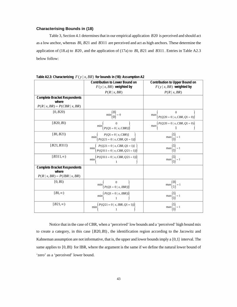
43

Characterising Bounds in (18) Table 3, Section 4.1 determines that in our empirical application 20B is perceived and should act

as a low anchor, whereas 1, 21B B and 311B are perceived and act as high anchors. These determine the

application of (18.a) to 20B , and the application of (17a) to 1, 21B B and 311B . Entries in Table A2.3

below follow:


( | , )F y x BR weighted by ( | , )P R x BR

Contribution to Upper Bound on ( | , )F y x BR weighted by

( | , )P R x BR Complete Bracket Respondents

where ( | , ) ( | , )P R x BR P CBR x BR=

[0, 20)B { } 0min00 = { }0

max( 20 0 | , , 1 0)P Q x CBR Q= =

[ 20, 1)B B { }0min

( 1 0 | , )]P Q x CBR= { }( 20 0 | , , 1 0)

max 1P Q x CBR Q= =

[ 1, 21)B B { }( 1 0 | , )]min

( 21 0 | , , 1 1)]P Q x CBR

P Q x CBR Q=

= = { } 1max

11 =

[ 21, 311)B B { }( 21 0 | , , 1 1)]min

( 311 0 | , , 21 1)]P Q x CBR Q

P Q x CBR Q= == =

{ } 1max11 =

[ 311, )B ∞ { }( 311 0 | , , 21 1)]min

1P Q x CBR Q= = { } 1max

11 =


( | , ) ( | , )P R x BR P IBR x BR=

[0, 1)B { }0min

( 1 0 | , )]P Q x IBR= { } 1max

01 =

[ 1, )B ∞ { }( 1 0 | , )]min

1P Q x IBR= { } 1max

11 =

[ 21, )B ∞ { }( 21 0 | , , 1 1)]min

1P Q x IBR Q= = { } 1max

11 =

Notice that in the case of CBR, when a ‘perceived’ low bounds and a ‘perceived’ high bound mix

to create a category, in this case [ 20, 1)B B , the identification region according to the Jacowitz and

Kahneman assumption are not informative, that is, the upper and lower bounds imply a [0,1] interval. The

same applies to [0, 1)B for IBR, where the argument is the same if we define the natural lower bound of

‘zero’ as a ‘perceived’ lower bound.

44


Table A2.4: Characterizing ( | , )F y x BR for bounds in (22): Assumption A3 Contribution to Lower Bound on ( | , )F y x BR

weighted by ( | , )P R x BR Contribution to Upper Bound on ( | , )F y x BR

weighted by ( | , )P R x BR Complete Bracket

Respondents where

( | , )

( | , )

P R x BR

P CBR x BR=

[0, 20)B { }0min

( 20 0 | , , 1) ( 1 0 | , )]P Q x CBR Q P Q x CBR= = { }0

max( 1 0 | , )P Q x CBR=

[ 20, 1)B B { }( 20 0 | , , 1) ( 1 0 | , )]min

( 1 0 | , )P Q x CBR Q P Q x CBR

P Q x CBR= =

= { }( 1 0 | , )

max( 1 0 | , )

P Q x CBRP Q x CBR

==

[ 1, 21)B B { }( 1 0 | , )min

( 1 0 | , )P Q x CBRP Q x CBR

==

( 1 0 | , )( 1 0 | , )max

( 21 0 | , , 1 1) ( 1 1 | , )

P Q x CBRP Q x CBR

P Q x CBR Q P Q x CBR

== +

+ = = =

⎧ ⎫⎪ ⎪⎨ ⎬⎪ ⎪⎩ ⎭

[ 21, 311)B B ( 1 0 | , )( 1 0 | , )min

( 21 0 | , , 1 1) ( 1 1 | , )

P Q x CBRP Q x CBR


== +

+ = = =

⎧ ⎫⎪ ⎪⎨ ⎬⎪ ⎪⎩ ⎭

( 1 0 | , )

( 21 0 | , , 1 1) ( 1 1 | , )max

( 21 0 | , )

( 311 0 | , , 21 1) ( 21 1 | , )

P Q x CBR

P Q x CBR Q P Q x CBRP Q x CBR


= +

+ = = == +

+ = = =

⎧ ⎫⎪ ⎪⎪ ⎪⎨ ⎬⎪ ⎪⎪ ⎪⎩ ⎭

[ 311, )B ∞ ( 1 0 | , )

min ( 21 0 | , , 1 1) ( 1 1 | , )1

P Q x CBR


= +

+ = = =

⎧ ⎫⎪ ⎪⎨ ⎬⎪ ⎪⎩ ⎭

( 21 0 | , )

max ( 311 0 | , , 21 1) ( 21 1 | , )1

P Q x CBR


= +

+ = = =

⎧ ⎫⎪ ⎪⎨ ⎬⎪ ⎪⎩ ⎭

Complete Bracket Respondents

where ( | , )

( | , )

P R x BR

P IBR x BR=

[0, 1)B { }0min

( 1 0 | , )P Q x IBR= { }0

max( 1 0 | , )P Q x IBR=

[ 1, )B ∞ { }( 1 0 | , )min 1

P Q x IBR= { }( 1 0 | , )max 1

P Q x IBR=

[ 21, )B ∞ { }( 1 0 | , )min

1P Q x CBR= ( 1 0 | , )

max ( 21 0 | , , 1 1) ( 1 1 | , )1

P Q x CBR


= +

+ = = =

⎧ ⎫⎪ ⎪⎨ ⎬⎪ ⎪⎩ ⎭

Documents

Identification and Estimation with Partial Respondents and