Estimation of Partial Differential Equations with Applications in

Finance∗

Dennis Kristensen†, London School of Economics

June 7, 2004

Abstract

Linear parabolic partial differential equations (PDE’s) and diffusion models are closely linkedthrough the celebrated Feynman-Kac representation of solutions to PDE’s. In asset pricing theory,this leads to the representation of derivative prices as solutions to PDE’s. We give a number ofexamples of this, including the pricing of bonds and interest rate derivatives. Very often derivativeprices are calculated given preliminary estimates of the diffusion model for the underlying variable.We demonstrate that the derivative prices are consistent and asymptotically normally distributedunder general conditions. We apply this result to three leading cases of preliminary estimators:Nonparametric, semiparametric and fully parametric ones. In all three cases, the asymptotic distri-bution of the solution is derived. Our general results have other applications in asset pricing theoryand in the estimation of diffusion models; these are also discussed.

∗This paper is part of my PhD-thesis at the LSE. I would like to thank my supervisor, Oliver Linton, for valuable

suggestions and comments. An earlier version of the paper was presented at Department of Statistics and Operations

Research, University of Copenhagen.†E-mail: d.kristensen@lse.ac.uk Address: R4z19C, FMG, London School of Economics, Houghton Street, London

WC2A 2AE, United Kingdom

1

1 Introduction

Partial differential equations (PDE’s) are used in fields as diverse as physics, biology, economics, and

finance to model and analyse dynamic systems. One class of PDE’s which has received particular

attention are the linear parabolic ones (LPDE’s). These make up a large class of PDE’s which is of a

sufficiently simple structure such that a thorough analysis of them is possible, see e.g. Friedman (1964)

and Evans (1998) for an introduction and detailed analysis of their properties.

One area where LPDE’s play an essential role is in asset pricing theory in general and in the pricing

of financial derivatives in particular. The latter are securities whose pay-off is contingent of the value

of an underlying variable, this for example being a stock price or an interest rate. The option pricing

literature was revolutionised by the groundbreaking work of Black and Scholes (1973) and Merton (1973,

1976). Assuming that the underlying asset follows a geometric Brownian motion and that trading takes

place in continuous time, they derived the price of an option as the solution to a LPDE using hedging

and no-arbitrage arguments. This result has since then been generalised in various directions. In

particular, the restriction that the fundamental asset price follows a geometric Brownian motion can

be weakened to allow for basically any diffusion type process.

In the above framework, the option price is a functional of the so-called drift and diffusion term,

these being functions characterising the diffusion process that the underlying asset is assumed to follow.

Empirical applications of these option pricing formulae therefore almost always involve some sort of

calibration of the drift and diffusion term. These calibrated terms can then substituted into the LPDE

in place of the true but unknown ones, and the option price solved for. The calibration is often done by

statistical estimation based on historical data. The implied option prices therefore inherit the statistical

uncertainty associated with the estimated drift and diffusion term. It will be valuable to be able to

measure how the estimation error (e.g. in terms of standard errors) in the drift and diffusion term

affects the resulting option prices. This will allow one to evaluate the accuracy of the estimated prices.

Moreover, such results can be used to construct a direct statistical test of the option price model by

comparing the estimated prices with the observed ones.

We give general results for the asymptotic properties of the implied option prices given preliminary

estimators of the drift and diffusion term. The implied/estimated price is obtained as the solution to a

LPDE where the preliminary estimators have been plugged in. We shall here show that the estimated

solution will be consistent when the preliminary estimators are. We also give general conditions under

which the solution will be asymptotically normal distributed. In the option pricing framework, this

means that the estimated prices are consistent if the drift and diffusion estimators for the underlying

asset price diffusion are. Furthermore, we are able to calculate standard errors for the prices. We first

state this result under fairly general conditions. We then verify these conditions for three specific types

of preliminary estimators, a parametric, a semiparametric and a nonparametric one, and derive the

asymptotic distribution in each case.

Similar results to the ones derived here can be found elsewhere in the literature. In the Black-

Scholes model, the statistical properties of option prices given preliminary estimates of the diffusion

term has been considered in a number of studies, see e.g. Boyle and Ananthanarayanan (1977) and

Ncube and Satchell (1997). In a very general setting, Lo (1986) derived the asymptotic properties of

2

the implied option prices given preliminary parametric estimates of the drift and diffusion function.

However, this was done under high-level conditions, and it was not verified that these actually hold.

Furthermore, he was not able to give closed form expressions for the asymptotic distribution. Interest

rate derivative pricing given kernel estimators of the short rate model was considered in Aït-Sahalia

(1996a) and Jiang (1998). Our results extend these results to basically any asset pricing model which

is driven by a finite number of state variables, and virtually any estimator of the drift and diffusion

term in the model in question. In particular, our results include multi-factor interest rate models and

stochastic volatility models. In the parametric case, we are able to derive an explicit expression of the

asymptotic distribution which allows one to estimate this. In the general case, we are not able to do

this; we are however still able to define a simple estimator of the asymptotic distribution which should

be consistent.

Other applications of our general results are also available in the econometric analysis of diffusion

models, e.g. GMM-type estimators [Bibby and Sørensen 1995, Duffie and Singleton 1993] and the

estimation using observed option prices. We give a brief discussion of these applications.

Studies of solutions to (partial) differential equations given preliminary estimates of the driving

coefficients are found elsewhere in the literature. Hausman and Newey (1995) consider a non-linear

ODE and derive the asymptotic properties of an estimator of the solution when a preliminary estimator

of the driving function is available. Vanhems (2003) deals with a similar problem where a nonlinear

ODE depends on a conditional mean function. The conditional mean is then estimated by kernel

methods, and the associated estimated solution is analysed. PDE’s have also received some attention,

in particular in the financial econometrics literature. In Aït-Sahalia (1996a), the estimation of interest

rate derivative prices is treated given preliminary semiparametric estimators of the drift and diffusion

function of the short-term interest rate. His analysis is based on a deterministic characterisation of

the solution to the PDE as given in Friedman (1964), which he analyses using the functional delta

method of Aït-Sahalia (1993). Jiang (1998) follows the same approach when analysing the properties

of estimated option prices given fully nonparametric estimators of the drift and diffusion term. Finally,

Chow et al (1999) also consider nonparametric estimation in the context of PDE’s. But while we are

concerned with the estimation of the solution given preliminary estimators of coefficients entering the

PDE, they assume that the solution of the PDE has been observed with error, and then use this to

estimate parameters entering the PDE.

A very nice feature of the class of LPDE’s is the probabilistic interpretation which a solution to any

PDE of this type can be given: Under weak regularity conditions the solution can be characterised as the

conditional moment of a solution to an associated diffusion process. This is the celebrated Feynman-Kac

Representation of solutions to LPDE’s. This is exactly the link that allows one to translate the option

price as the discounted expected value of the future price into the solution to a LPDE. Our analysis of

the estimated solution is based on this stochastic representation as a conditional expectation involving

a diffusion process. This approach has proved very fruitful in the analysis of various other problems

related to this type of PDE’s, see e.g. Freidlin (1985) for an exposition. So instead of directly working

with the PDE of interest, we shall focus on a certain class of conditional moments of the associated

stochastic differential equation (SDE) in terms of which the solution to the PDE can be expressed.

One advantage of this approach is that while in the general case it is difficult to set up conditions for

3

the existence of a global solution to the PDE, the conditional moments of the SDE of interest will be

well-defined under weak conditions. Another is that a closed form expression of the conditional moment

is available which facilitates the statistical analysis of the estimator.

Once the general asymptotic result has been established, we apply it to three leading preliminary

estimators: Fully parametric estimators of the drift and diffusion term (including MLE and GMM),

semiparametric ones (see Aït-Sahalia 1996a and Chapter 4 ), and fully nonparametric ones (see Jiang

and Knight 1997 and Bandi and Phillips 2003). In all three cases, we are able to derive the convergence

rate and the asymptotic distribution of the solution. In particular, we demonstrate that even if non- and

semiparametric preliminary estimators are used, the associated solution will converge with parametric

rate. This appealing result follows from the higher level of regularity/smoothness of the solution to the

PDE compared to the preliminary estimators. This is a well-known phenomenon found elsewhere in

the literature on nonparametric estimation. One important consequence is that if the end goal of the

econometric analysis of the asset price model is the pricing of derivatives, one will asymptotically in

many cases be better off using non- and semiparametric estimators: These allow for a higher level of

flexibility without slowing down the rate of convergence of the solution. Of course, if one has correctly

specified a parametric model of the underlying SDE, a parametric estimator of the solution will in most

cases enjoy higher efficiency and better finite sample properties than the nonparametric one. Moreover,

inherent in nonparametric estimation is a problem of choosing some smoothing parameter; this problem,

one does not face in a parametric setting.

The study is organised as follows. In the next section we first present the class of PDE’s of interest

and derive some useful properties of these; we then discuss various applications to finance and estimation

of diffusions. In Section 3, a general result concerning consistency and asymptotic normality is first

presented which is then applied to the aforementioned three types of estimators. These econometric

results are then put into the framework of derivative pricing in Section 4, which also contains a discussion

on the application of our results to GMM-type estimation of diffusion models and estimation based on

observed option prices. Section 5 concludes. All proofs and lemmas have been relegated to appendix

A and B respectively.

2 Linear Parabolic Partial Differential Equations

We shall in the following introduce the class of linear parabolic PDE’s together with the concept of

generalised solutions to these. We give conditions for these to be well-defined. The section ends with

a presentation of the various applications of LPDE’s to finance and estimation of diffusion models.

For any two functions µ : [0,∞)×Rq 7→ Rq and σ2 : [0,∞)×Rq 7→ Rq×q, we define the linear secondorder differential operator

Lt (u) =

qXi=1

µi (t, x)∂u

∂xi+1

2

qXi,j=1

σ2ij (t, x)∂2u

∂xi∂xj.

This is normally referred to as the infinitesimal generator, c.f. Karatzas and Shreve (1991, p. 281). For

4

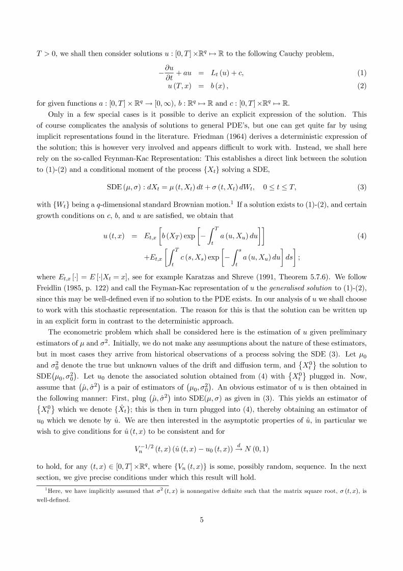
T > 0, we shall then consider solutions u : [0, T ]×Rq 7→ R to the following Cauchy problem,

−∂u∂t+ au = Lt (u) + c, (1)

u (T, x) = b (x) , (2)

for given functions a : [0, T ]×Rq → [0,∞), b : Rq 7→ R and c : [0, T ]×Rq 7→ R.Only in a few special cases is it possible to derive an explicit expression of the solution. This

of course complicates the analysis of solutions to general PDE’s, but one can get quite far by using

implicit representations found in the literature. Friedman (1964) derives a deterministic expression of

the solution; this is however very involved and appears difficult to work with. Instead, we shall here

rely on the so-called Feynman-Kac Representation: This establishes a direct link between the solution

to (1)-(2) and a conditional moment of the process Xt solving a SDE,

SDE (µ, σ) : dXt = µ (t,Xt) dt+ σ (t,Xt)dWt, 0 ≤ t ≤ T, (3)

with Wt being a q-dimensional standard Brownian motion.1 If a solution exists to (1)-(2), and certaingrowth conditions on c, b, and u are satisfied, we obtain that

u (t, x) = Et,x

·b (XT ) exp

·−Z T

ta (u,Xu) du

¸¸(4)

+Et,x

·Z T

tc (s,Xs) exp

·−Z s

ta (u,Xu)du

¸ds

¸;

where Et,x [·] = E [·|Xt = x], see for example Karatzas and Shreve (1991, Theorem 5.7.6). We follow

Freidlin (1985, p. 122) and call the Feyman-Kac representation of u the generalised solution to (1)-(2),

since this may be well-defined even if no solution to the PDE exists. In our analysis of u we shall choose

to work with this stochastic representation. The reason for this is that the solution can be written up

in an explicit form in contrast to the deterministic approach.

The econometric problem which shall be considered here is the estimation of u given preliminary

estimators of µ and σ2. Initially, we do not make any assumptions about the nature of these estimators,

but in most cases they arrive from historical observations of a process solving the SDE (3). Let µ0and σ20 denote the true but unknown values of the drift and diffusion term, and

©X0t

ªthe solution to

SDE¡µ0, σ

20

¢. Let u0 denote the associated solution obtained from (4) with

©X0t

ªplugged in. Now,

assume that¡µ, σ2

¢is a pair of estimators of

¡µ0, σ

20

¢. An obvious estimator of u is then obtained in

the following manner: First, plug¡µ, σ2

¢into SDE(µ, σ) as given in (3). This yields an estimator of©

X0t

ªwhich we denote Xt; this is then in turn plugged into (4), thereby obtaining an estimator of

u0 which we denote by u. We are then interested in the asymptotic properties of u, in particular we

wish to give conditions for u (t, x) to be consistent and for

V −1/2n (t, x) (u (t, x)− u0 (t, x))d→ N (0, 1)

to hold, for any (t, x) ∈ [0, T ]×Rq, where Vn (t, x) is some, possibly random, sequence. In the nextsection, we give precise conditions under which this result will hold.

1Here, we have implicitly assumed that σ2 (t, x) is nonnegative definite such that the matrix square root, σ (t, x), is

well-defined.

5

Since the solutions in most cases cannot be written on an explicit form, numerical methods are

normally used to solve the solution to the PDE (1)-(2). Hull (1997, Chapter 15) provides an overview

of a number of numerical methods used in finance. The two most popular methods is the so-called

finite-difference method and Monte Carlo methods. A thorough treatment of numerical solutions of

PDE’s using finite difference methods can be found in Ames (1992). Alternatively, the solution u

can be obtained by the use of Monte Carlo methods; these are normally based on the Feynman-Kac

representation. The Monte Carlo simulations can be done in the following manner: Let X(i)s |t ≤ s ≤

T, i = 1, ...,N , be N independent simulated paths of the SDE (3) with initial condition Xt = x. We

then approximate u (t, x) by

u(N) (t, x) =1

N

NXi=1

·b³X(i)T

´exp

·−Z T

ta³u,X(i)

u

´du

¸¸(5)

+1

N

NXi=1

·Z T

tc³s,X(i)

s

´exp

·−Z s

ta³u,X(i)

u

´du

¸ds

¸.

Let P ∗ denote the probability measure that we simulate under. Then EP ∗ £u(N) (t, x)¤ = u (t, x), and,

by the strong Law of Large Numbers, u(N) (t, x)→P ∗−a.s. u (t, x) as N →∞. It is however not possibleto obtain an exact continuous sample path of this type of stochastic processes; instead one often derives

an approximate discrete time version of (3) from which one simulates. This approximate model can be

chosen arbitrarily close to the actual one. For an overview of simulations of SDE’s, we refer to Kloeden

and Platen (1999).

We now wish to discuss the question of existence and uniqueness of the generalised solution and

derive some of its properties. These will prove useful in the subsequent section when we deal with

the econometric problem in question. Sufficient conditions for a solution to (1)-(2) can be found in

Friedman (1964, Section I.4) and Evans (1998, Chapter 5). In the following, we construct a set of

function pairs, D, such that for any¡µ, σ2

¢∈ D, the associated generalised solution u exists and is

sufficiently well-behaved. This is done by restricting D in the following manner:

Definition The space D consists of all function pairs¡µ, σ2

¢where

1. µ and σ2 are twice continuously differentiable in x such that:

(a) There exists K > 0 such that

k∂αxµ (t, x)k ≤ K (1 + kxk) ,°°∂αxσ2 (t, x)°° ≤ K (1 + kxk) ,

for all (t, x) ∈ [0, T ]×Rq and |α| ≤ 2.(b) For all N ≥ 1, there exists KN > 0 such that

kµ (t, x)− µ (t, y)k ≤ KN kx− yk ,°°σ2 (t, x)− σ2 (t, y)

°° ≤ KN kx− yk ,

for all t ∈ [0, T ] and kxk , kyk ≤ N .

2. There exists a constant σ2 > 0 such thatPq

i,j=1 σ2ij (t, x) yiyj ≥ σ2 kyk2 for all y ∈ Rq and

(t, x) ∈ [0, T ]×Rq.

6

Observe that D is a well-defined function space. For any¡µ, σ2

¢∈ D and any initial condition,

X0 = X∗, which is independent of Wt and satisfies EhkX∗k2

i<∞, there exists an associated unique

strong solution to (3), c.f. Friedman (1975, Theorem 5.2.2). Furthermore, if EhkX∗k2p

i<∞, for some

p ≥ 1,EhkXtk2p

i≤³1 +E

hkX∗k2p

i´eC

∗t (6)

for 0 ≤ t ≤ T , where C∗ = C∗ (K, p, T ), c.f. Friedman (1975, Theorem 5.2.3). For q = 1, a weaker

sufficient condition for existence and uniqueness is that µ and σ2 are continuously differentiable and

σ2 (·) > 0, c.f. Karatzas and Shreve (1991, Theorem 5.5.15 and Corollary 5.3.23). The bound in (6) doesnot necessarily hold in this case however. For q > 1, weaker conditions for existence and uniqueness

can be found in Meyn and Tweedie (1993). Most likely the results presented in the following hold for¡µ, σ2

¢situated in a larger function space, but for simplicity we shall restrict them to belong to D.

The existence and uniqueness results for Xt hold without the differentiability conditions on µ and σ;these are used when we derive the asymptotic properties of u.

In the following we consider a fixed pair¡µ0, σ

20

¢∈ D, and denote the associated diffusion process

by©X0t

ª. We also fix the initial condition of

©X0t

ªat some given random variable, X∗. First we define

Lp (X∗, [0, T ]×Rq) as the space of functions f : [0, T ]×Rq 7→ R for which E

hR T0

¯f¡t,X0

t

¢¯pdti<∞.

Next, we introduce a Sobolev-like spaceWm,p =Wm,p (X∗, [0, T ]×Rq) for any p ≥ 1 andm ≥ 0. This isdefined as the space of functions f : [0, T ]×Rq 7→ Rwhich arem times continuously differentiable in their

second argument and with ∂αx f ∈ Lp (X∗, [0, T ]×Rq) for any α ∈ 0, ..., kq with |α| =

Pqi=1 αi = k,

0 ≤ k ≤ m. We equip the space with the norm

kfkm,p =

X|α|≤m

E

·Z T

0|∂αx f

¡t,X0

t

¢|pdt]

¸1/p .Observe that Wm,2 is a Hilbert space with inner product

hf, gim =X|α|≤m

E

·Z T

0∂αx f

¡t,X0

t

¢∂αx g

¡t,X0

t

¢dt

¸(7)

and that W 0,p = Lp (X∗, [0, T ]×Rq). Combining the above results, we observe that if (i) f has

m derivatives in its second argument and these satisfies ||∂αx f (t, x) || ≤ C (1 + kxkr), |α| ≤ m, (ii)¡µ0, σ

20

¢∈ D and (iii) E

hkX∗kp∗

i< ∞, then f ∈ Wm,p with p = p∗/r . In particular, for any¡

µ, σ2¢∈ D,

¡µ, σ2

¢∈W 2,p ×W 2,p with p ≤ p∗.

We impose the following conditions on the functions a, b, and c:

Condition 1 For some r ≥ 1, |∂αxa (t, x)| ≤ C (1 + kxkr), |∂αx b (t, x)| ≤ C (1 + kxkr) and |∂αx c (t, x)| ≤C (1 + kxkr), |α| ≤ 2.

It is not always the case in our applications that the functions are differentiable as assumed here.

We conjecture that the results also hold in this case. All the following results are derived under the

implicitly maintained assumption that Condition 1 holds. The first result ensures that u exists and is

well-defined for suitable choices of µ and σ2:

7

Theorem 1 For any¡µ, σ2

¢∈ D, the associated generalised solution u exists. Furthermore, |∂αxu (t, x)| ≤

C (T ) (1 + kxkr) for |α| ≤ 2. In particular, u ∈W 2,p for any initial condition X∗ with E [kX∗kpr] <∞.

2.1 Applications in Finance

One particular area where PDE’s of the linear parabolic type is widely used is in asset pricing theory in

general and derivative pricing in particular. Derivatives are securities whose pay-off depends on some

underlying variable, e.g. the price of a stock or an interest rate, with the most well-known example being

options. Financial derivatives play an important role in the financial markets, and have consequently

received great attention in the finance literature. Since the seminal work by Black-Scholes (1973)

and Merton (1973), diffusion processes have played a prominent part in the asset pricing literature.

Assuming that the fundamental asset prices solve an SDE, one is able to derive closed form solutions

of derivative prices. In fact, one of the main results is that the price of the derivative is the solution

to a PDE in the class considered here. Below, we give a brief overview of the various fields where our

results can be applied. These examples illustrate the wide range of applications that parabolic PDE’s

have.

We first introduce the necessary notation. We fix the probability space (P,Ω,F) with an associatedfiltration Ft. Here P denotes the physical measure under which we observe the processes introduced

in the following.

Example 1: A General Asset Pricing Model. Consider a riskless asset βt given by

dβt = rtβtdt,

for some adapted short-term interest rate process, rt, see Chapter 2 for a discussion of these. Weare also given N risky traded assets, each having an associated price process S(i)t , i = 1, ...,N . Weassume that the process St, St = (S(1)t , ..., S

(N)t )>, solves a SDE,

dSt = µS (t, St) dt+ σS (t, St) dwSt , (8)

where©WS

t

ªis a N-dimensional standard Brownian motion. Each asset i has also an associated

dividend stream d(i)t , i = 1, ...,N , which we collect in dt, dt = (d(1)t , ..., d

(N)t )>. Given the existence

of an equivalent martingale measure, Q,2 the price process then satisfies

St = EQt

·exp

·−Z T

trsds

¸ST +

Z T

texp

·−Z s

trsdu

¸dsds

¸, (9)

where St has dynamicsdSt = rtStdt+ σS (t, St)dW

St (10)

under Q, see for example Duffie (1996, Chapter 6 and 8). Observe that µS does not enter the dynamics

of St under Q, and therefore has no influence on the option prices. Assume that rt and dt alsosolve SDE’s under Q,

drt = µr (t, rt) dt+ σr (t, rt) dWrt ,

ddt = µD (t, St)dt+ σD (t, St) dWDt .

2We shall not discuss conditions for the existence (and uniqueness) of Q, and merely assume its existence.

8

Then by defining

Xt =³S>t , d

>t , rt

´>, Wt = (W

St ,W

Dt ,W r

t )>,

µ (t, x) =³rS>, µ>D (t, S) , µr (t, r)

´>, σ (t, x) = diag (σS (t, S) , σD (t, S) , σr (t, r)) ,

we observe that the pricing formula (9) takes the form of (4). More advanced models for the short term

interest rate as presented below can without any problems be allowed for.

Example 1.1: The Black-Scholes Model. A special case of the above model is the (extended) Black-

Scholes model where we have one risky asset (N = 1), say a stock, and a derivative on this stock. At

time of maturity T , the derivative pays off b (ST ). From (9), the following expression of the price of

the derivative at time t, Πt (T ), presents itself,

Πt (T ) = EQt

·exp

·−Z T

trsds

¸PT (T )

¸= EQ

t

·exp

·−Z T

trsds

¸b (ST )

¸,

where St solves (10) under Q. In the classic Black-Scholes model, it is assumed that the short-terminterest rate is constant, rt ≡ r > 0, and that St is a geometric Brownian motion under P ; that is,

dSt = µStdt+ σStdwSt .

We then consider a call-option where the pay-off function is b (x) = max x−K, 0 with K being the

strike price.3 In this case, the above conditional expectation can be shown to satisfy

Πt (T ) = SΦ (d1)−Ke−r(T−t)Φ (d2) ,

where Φ (·) is the cumulative density function of the standard normal distribution and

d1 =log (S/K) +

¡r + σ2/2

¢(T − t)

σ√T − t

, d2 = d1 − σ√T − t.

In the general case with more complex dynamics of St and/or stochastic interest rates, an explicitexpression for Πt (T ) is not available. Instead, one has to rely on numerical methods to calculate the

actual prices as discussed earlier.

Example 1.2: Stochastic Volatility Models. The classic Black-Scholes model is not able to match ob-

served option prices very well. To deal with this empirical shortcoming stochastic volatility models

were introduced, see e.g. Ghysels et al (1996) for a review. We still consider some stock price process

St but we now assume thatdSt = µS (St) dt+ σS (St, vt) dw

St , (11)

where vt is non-traded/unobserved process solving

dvt = µv (vt) dt+ σv (vt) dwvt (12)

and, for simplicity,©wSt

ªand wv

t are mutually independent standard Brownian motion.4 This is anextension of the classic Black-Scholes model where vt can be interpreted as a stochastic volatilityterm. In this setting, (9) is still valid but now

dSt = rStdt+ σS (St, vt) dWSt ,

3Observe that b is not differentiable here. We conjecture that the results still hold for this case however.4We can also allow for St entering the SDE for vt, and also that vt enters the drift function µS .

9

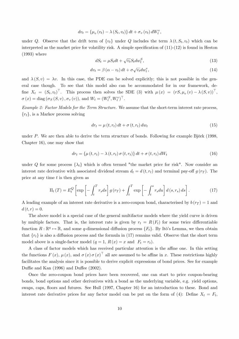
dvt = µv (vt)− λ (St, vt) dt+ σv (vt) dWvt ,

under Q. Observe that the drift term of vt under Q includes the term λ (t, St, vt) which can be

interpreted as the market price for volatility risk. A simple specification of (11)-(12) is found in Heston

(1993) where

dSt = µStdt+√vtStdw

St , (13)

dvt = β (α− vt)dt+ σ√vtdw

vt , (14)

and λ (S, v) = λv. In this case, the PDE can be solved explicitly; this is not possible in the gen-

eral case though. To see that this model also can be accommodated for in our framework, de-

fine Xt = (St, vt)>. This process then solves the SDE (3) with µ (x) = (rS, µv (v)− λ (S, v))>,

σ (x) = diag (σS (S, v) , σv (v)), and Wt = (WSt ,W

vt )>.

Example 2: Factor Models for the Term Structure. We assume that the short-term interest rate process,

rt, is a Markov process solving

drt = µ (t, rt)dt+ σ (t, rt)dwt (15)

under P . We are then able to derive the term structure of bonds. Following for example Björk (1998,

Chapter 16), one may show that

drt = µ (t, rt)− λ (t, rt)σ (t, rt) dt+ σ (t, rt)dWt (16)

under Q for some process λt which is often termed "the market price for risk". Now consider aninterest rate derivative with associated dividend stream dt = d (t, rt) and terminal pay-off g (rT ). The

price at any time t is then given as

Πt (T ) = EQt

·exp

·−Z T

trsds

¸g (rT ) +

Z T

texp

·−Z s

trsdu

¸d (s, rs)ds

¸. (17)

A leading example of an interest rate derivative is a zero-coupon bond, characterised by b (rT ) = 1 and

d (t, r) = 0.

The above model is a special case of the general multifactor models where the yield curve is driven

by multiple factors. That is, the interest rate is given by rt = R (Ft) for some twice differentiable

function R : Rq 7→ R, and some q-dimensional diffusion process Ft. By Itô’s Lemma, we then obtainthat rt is also a diffusion process and the formula in (17) remains valid. Observe that the short termmodel above is a single-factor model (q = 1, R (x) = x and Ft = rt).

A class of factor models which has received particular attention is the affine one. In this setting

the functions F (x), µ (x), and σ (x)σ (x)> all are assumed to be affine in x. These restrictions highly

facilitates the analysis since it is possible to derive explicit expressions of bond prices. See for example

Duffie and Kan (1996) and Duffee (2002).

Once the zero-coupon bond prices have been recovered, one can start to price coupon-bearing

bonds, bond options and other derivatives with a bond as the underlying variable, e.g. yield options,

swaps, caps, floors and futures. See Hull (1997, Chapter 16) for an introduction to these. Bond and

interest rate derivative prices for any factor model can be put on the form of (4): Define Xt = Ft,

10

a (t, x) = R (x), b (x) = g (R (x)), c (t, x) = d (t, F (x)); we then easily see that (17) takes the desired

form.

Example 3: The Heath-Jarrow-Morton Model. In the Heath-Jarrow-Morton (1992) framework, the

forward rate structure is modelled instead of the short rate. Let ft (T ) denote the instantaneous

forward rate with maturity T contracted at time t. This is defined as

ft (T ) =∂ logBt (T )

∂T

where Bt (T ) is the price of a zero-coupon bond with maturity date T . One can reversely write

Bt (T ) = exph−R Tt ft (s) ds

i. In particular, the short rate satisfies rt = ft (t). We assume the following

dynamics of ft (T ) under Q,

dft (T ) = µt (T ) dt+ σt (T ) dWt,

where Wt is a q-dimensional Brownian motion, while µt (T ) and σt (T ) are adapted stochasticprocesses. The assumption of no-arbitrage implies that

µt (T ) = σt (T )

Z T

tσt (s)

> ds,

c.f. Björk (1998, p. 269). Furthermore, the bond prices have the following dynamics,

dBt (T ) = rtBt (T ) dt+ σ∗t (T )Bt (T ) dWt,

where σ∗t (T ) =R Tt σs (T )ds. Assuming that µt (T ) = µ (t,Xt;T ) and σt (T ) = σ (t,Xt;T ) for some

finite-dimensional vector of state-variables Xt, the above pricing formula takes the form of (4).

2.2 Estimation of Diffusion Models

The type of partial differential equations in consideration here also appear in other areas. In the

following, we give a brief discussion of their applications in the estimation of diffusions. The literature

on the estimation of diffusion models is very large and still growing. One particular branch of this

literature is concerned with estimation given discrete observations of the process, e.g. daily, weekly

or monthly observations. This is the most realistic setting but also the least tractable; in particular

the natural estimator, the MLE, proves to be difficult to implement. A large number of alternative

estimators have been proposed as a result. But the asymptotic properties of these have either only been

conjectured at or derived under high-level conditions. The results derived in the next section enable

us to validate these high-level conditions. In the following, we shall present a number of estimation

methods and discuss what is needed for the estimator to have the desired asymptotic properties. We

shall only discuss these issues in a parametric framework, but it should be clear that our main results

also are applicable in a non- and semiparametric setting.

We assume that we have discrete observations from the following SDE,

dXt = µ (Xt; θ)dt+ σ (Xt; θ)dWt, (18)

for some unknown parameter θ ∈ Θ ⊆ Rd. In the following we discuss the estimation of θ.

11

Example 4: Estimation via Conditional Means. Since in many cases the transition density is of unknown

form, the model is often estimated using estimating equations. In particular, one often use regression

models of the form

b (Xi∆) = B¡X(i−1)∆; θ

¢+ εi

where B (x; θ) = Eθ [b (X∆) |X0 = x] is the conditional mean where we write Eθ [·] to indicate thedependence of the conditional mean on θ. Using this type of equations leads to GMM-type estimators

as considered in, amongst others, Bibby and Sørensen (1995), Chacko & Viceira (2003), Duffie and

Singleton (1993), Carrasco, Chernov, Florens & Ghysels (2002), Singleton (2001), Sørensen (1997). In

order to derive the asymptotics of this type of estimators, we need to show that B (x; θ) is smooth

and differentiable in θ. However, as noted earlier, an analytical expression of B (x; θ) often cannot

be derived and is calculated using either simulations or approximate methods. One easily realise that

B (x; θ) = u (0, x; θ) where u solves the LPDE

−∂u∂t= Lt (u; θ) , u (∆, x; θ) = b (x) .

One example is the estimator proposed in Bibby and Sørensen (1995). We define the so-called estimating

function,

Gn (θ) =1

n

nXi=1

g¡Xi∆|X(i−1)∆; θ

¢, g (y|x; θ) = α (x; θ)> b (y)−B (x; θ)

where b : Rq 7→ Rm and B are given above and α : Rq × Θ 7→ Rm×d is a weighting function. Theestimator is then chosen as the root, Gn(θ) = 0. An obvious choice is b1 (x) = x and b2 (x) = x2.

Example 5: Estimation via Observed Option Prices. Another application is in the estimation of the

parameter θ using observed derivative prices. We here present the estimation method using the extended

Black-Scholes model in Example 1.1 with constant interest rates, rt = r > 0, but the idea can easily

be adapted to other, more general models. For simplicity, we assume that we have observed over time

a series of prices for a specific option with pay-off function g and fixed time to maturity T > 0. So

no cross-sectional dimension is included. Let Pi denote the observed option prices and Xi theobserved stock price. Assuming that the option prices have been observed with errors (due to market

imperfections, observation errors etc.), we have the following regression model,

Pi = Π (Xi; θ) + εi, Π (x; θ) = e−rTEQθ [b (XT ) |X0 = x] .

The parameter θ may then be estimated by e.g. nonlinear least squares (assuming it is identified).

Again, for the estimator to be consistent and asymptotically normal distributed one normally has

to check that θ 7→ Π (x; θ) is continuous and differentiable. In the next section, we give regularity

conditions which ensures this.

3 Estimation of Partial Differential Equations

In this section, we shall assume that preliminary estimators¡µ, σ2

¢are available, and then give condi-

tions for the associated solution u to be consistent and asymptotically normal distributed.

12

We introduce the operator Γ : D 7→ U defined by

u (t, x) = Γ¡µ, σ2

¢(t, x) ,

where u is the solution to (1)-(2) with¡µ, σ2

¢plugged in. We assume that we have obtained estimators,¡

µ, σ2¢, of the true drift and diffusion term,

¡µ0, σ

20

¢. Given the definition of Γ, the true but unknown

solution to the PDE is given by

u0 = Γ¡µ0, σ

20

¢which we then estimate by

u = Γ¡µ, σ2

¢.

By an extension of Slutsky’s theorem from the Euclidean case to function spaces, the asymptotic

properties of u will then follow from the ones of¡µ, σ2

¢given that Γ is sufficiently smooth. Roughly

speaking, u will be consistent if¡µ, σ2

¢is so and Γ is continuous, while the asymptotic distribution

will be induced by the one of¡µ, σ2

¢given that Γ is (pathwise) differentiable w.r.t.

¡µ, σ2

¢. To

extend Slutsky’s Theorem to hold on function spaces we need to ensure that D and U can be equippedwith suitable norms. For now assume this is the case and let k·kD and k·kU denote the norms onD and U respectively. We then assume that our preliminary estimators satisfy

¡µ, σ2

¢∈ D with°°¡µ, σ2¢− ¡µ0, σ20¢°°D →P 0. Consistency of u = Γ

¡µ, σ2

¢will now follow by continuity of Γ since

this implies ku− u0kU =°°Γ ¡µ, σ2¢− Γ ¡µ0, σ20¢°°U →P 0. Assume that the pathwise derivative of Γ

w.r.t. µ and σ2 at¡µ0, σ

20

¢exists. We denote these ∇1Γ [dµ] and ∇2Γ

£dσ2

¤respectively and define

∇Γ£dµ, dσ2

¤= ∇1Γ [dµ] +∇2Γ

£dσ2

¤. Assuming that°°Γ ¡µ, σ2¢− Γ ¡µ0, σ20¢−∇Γ £µ− µ0, σ

2 − σ20¤°°U ≤ C

³kµ− µ0k2D +

°°σ2 − σ20°°2D´,

∇Γ will drive the asymptotic distribution under suitable conditions.The approach outlined above has been widely used in the literature when working with functionals

of nonparametric estimators. General result concerning the asymptotics of Γ when the preliminary

estimator is a kernel estimator can be found in Aït-Sahalia (1993). Examples of applications of this

approach to specific estimation problems can be found in Aït-Sahalia (1996a), Hausman and Newey

(1995), Jiang (1998) and Vanhems (2003).

All subsequent results will be derived under the following additional condition which implicitly will

be assumed throughout the remains of the chapter together with Condition 1:

Condition 2¡µ0, σ

20

¢∈ D

We first show that the functional Γ : D 7→ U is continuous.

Theorem 2 For any¡µ, σ2

¢∈ D,¯

Γ¡µ, σ2

¢(t, x)− Γ

¡µ0, σ

20

¢(t, x)

¯≤ CT (1 + kxkq)

nkµ− µ0k0,4 +

°°σ2 − σ20°°0,4

ofor X∗ = x. In particular,

ku− u0k0,1 ≤ CT (1 +E [kX∗kr])nkµ− µ0k0,4 +

°°σ2 − σ20°°0,4

o,

for r ≤ p∗.

13

We now derive an expression for the pathwise derivative of u w.r.t.¡µ, σ2

¢at¡µ0, σ

20

¢in the direction¡

dµ, dσ2¢=¡µ− µ0, σ

2 − σ20¢. Let ∇1Xt and ∇2Xt be given as in in (53) and (54) respectively

with ∇iX0 = 0, i = 1, 2. From Lemma 12, ∇1Xt and ∇2Xt are the pathwise derivatives w.r.t. µand σ2 respectively in the L2-sense. The pathwise derivative of Xt at

¡µ0, σ

20

¢in the direction

¡dµ, dσ2

¢in the L2-sense is then given by

∇Xt = ∇1Xt +∇2Xt.

The chain rule now implies that the pathwise derivative of Γ at¡µ0, σ

20

¢in the direction

¡dµ, dσ2

¢is

given by

∇Γ£dµ, dσ2

¤(t, x) (19)

= Et,x

·bx¡X0T

¢∇XT exp

·−Z T

ta¡u,X0

u

¢du

¸¸(20)

−Et,x

·b¡X0T

¢ Z T

tax¡u,X0

s

¢∇Xsds exp

·−Z T

ta¡s,X0

s

¢ds

¸¸+Et,x

·Z T

tcx¡s,X0

s

¢∇Xs exp

·−Z s

ta¡u,X0

u

¢du

¸ds

¸−Et,x

·Z T

tc¡s,X0

s

¢exp

·−Z s

ta¡u,X0

u

¢du

¸µZ s

tax¡u,X0

u

¢∇Xudu

¶ds

¸.

By construction, ∇Xt and thereby ∇Γ is linear in¡dµ, dσ2

¢. An alternative representation of ∇Γ is

as the solution, v, to the following LPDE,

−∂v∂t+ av = Lt (v) + c

£dµ, dσ2

¤(21)

v (T, x) = 0 (22)

where

c£dµ, dσ2

¤=

qXi=1

dµi∂u0∂xi

+1

2

qXi=1

dσ2ij∂2u0∂xi∂xj

,

and u0 = Γ¡µ0, σ

20

¢. The generalised solution of (21)-(22) is given as

∇Γ£dµ, dσ2

¤(t, x) = Et,x

·Z T

tc£dµ, dσ2

¤ ¡s,X0

s

¢exp

·−Z s

ta¡u,X0

u

¢du

¸ds

¸(23)

The following theorem shows that ∇Γ also has the desired properties discussed earlier:

Theorem 3 For any¡µ, σ2

¢∈ D, ∇Γ

£µ− µ0, σ

2 − σ20¤is well-defined and satisfies¯

u (t, x)− u0 (t, x)−∇Γ£µ− µ0, σ

2 − σ20¤(t, x)

¯≤ b (x, T ) kµ− µ0k21,4 +

°°σ2 − σ20°°21,4

and ¯∇Γ

£µ, σ2

¤(t, x)

¯≤ b (x, T )

³kµk20,2 +

°°σ2°°20,2

´,

with X∗ = x, where b (x, T ) = CTeCTh1 + kxk2q

i.

14

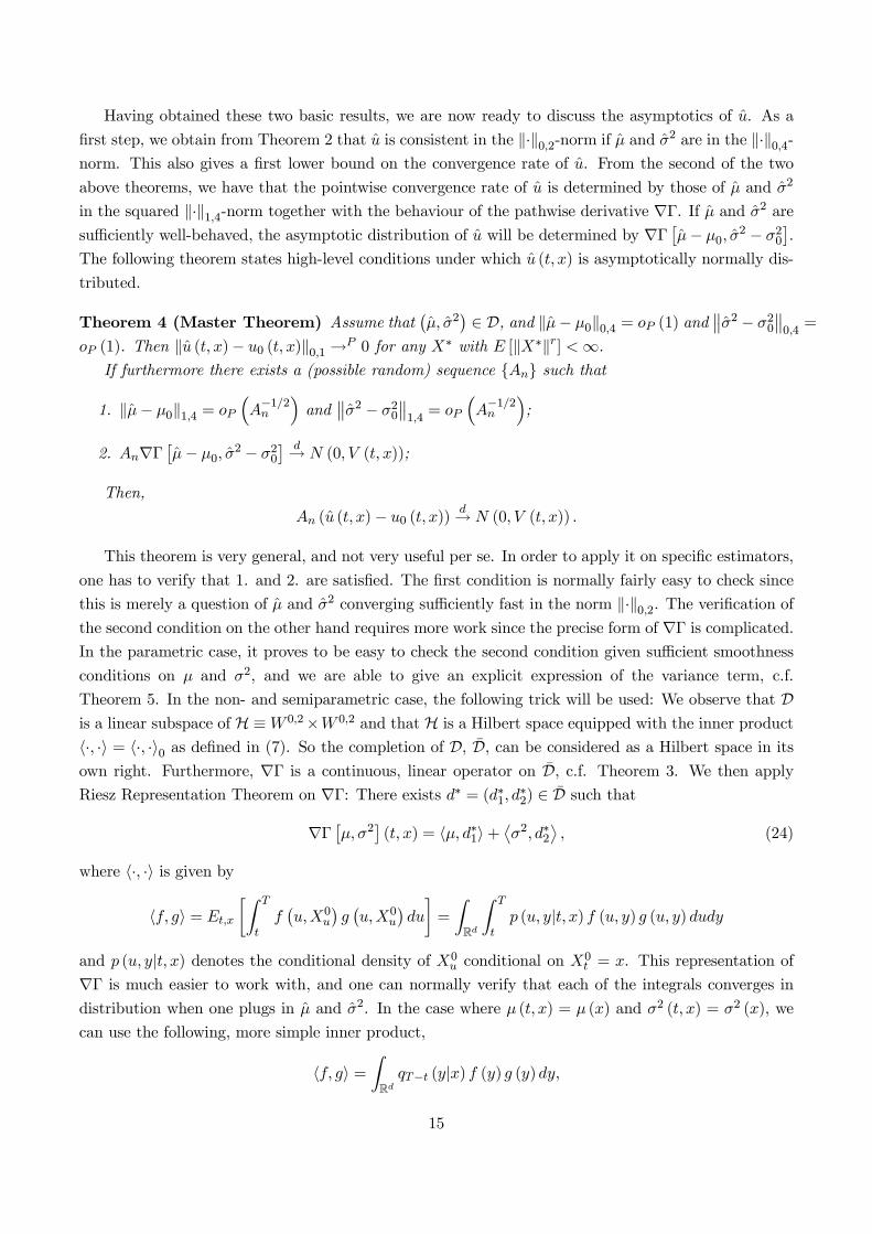
Having obtained these two basic results, we are now ready to discuss the asymptotics of u. As a

first step, we obtain from Theorem 2 that u is consistent in the k·k0,2-norm if µ and σ2 are in the k·k0,4-norm. This also gives a first lower bound on the convergence rate of u. From the second of the two

above theorems, we have that the pointwise convergence rate of u is determined by those of µ and σ2

in the squared k·k1,4-norm together with the behaviour of the pathwise derivative ∇Γ. If µ and σ2 are

sufficiently well-behaved, the asymptotic distribution of u will be determined by ∇Γ£µ− µ0, σ

2 − σ20¤.

The following theorem states high-level conditions under which u (t, x) is asymptotically normally dis-

tributed.

Theorem 4 (Master Theorem) Assume that¡µ, σ2

¢∈ D, and kµ− µ0k0,4 = oP (1) and

°°σ2 − σ20°°0,4=

oP (1). Then ku (t, x)− u0 (t, x)k0,1 →P 0 for any X∗ with E [kX∗kr] <∞.If furthermore there exists a (possible random) sequence An such that

1. kµ− µ0k1,4 = oP³A−1/2n

´and

°°σ2 − σ20°°1,4= oP

³A−1/2n

´;

2. An∇Γ£µ− µ0, σ

2 − σ20¤ d→ N (0, V (t, x));

Then,

An (u (t, x)− u0 (t, x))d→ N (0, V (t, x)) .

This theorem is very general, and not very useful per se. In order to apply it on specific estimators,

one has to verify that 1. and 2. are satisfied. The first condition is normally fairly easy to check since

this is merely a question of µ and σ2 converging sufficiently fast in the norm k·k0,2. The verification ofthe second condition on the other hand requires more work since the precise form of ∇Γ is complicated.In the parametric case, it proves to be easy to check the second condition given sufficient smoothness

conditions on µ and σ2, and we are able to give an explicit expression of the variance term, c.f.

Theorem 5. In the non- and semiparametric case, the following trick will be used: We observe that Dis a linear subspace of H ≡W 0,2×W 0,2 and that H is a Hilbert space equipped with the inner product

h·, ·i = h·, ·i0 as defined in (7). So the completion of D, D, can be considered as a Hilbert space in itsown right. Furthermore, ∇Γ is a continuous, linear operator on D, c.f. Theorem 3. We then apply

Riesz Representation Theorem on ∇Γ: There exists d∗ = (d∗1, d∗2) ∈ D such that

∇Γ£µ, σ2

¤(t, x) = hµ, d∗1i+

­σ2, d∗2

®, (24)

where h·, ·i is given by

hf, gi = Et,x

·Z T

tf¡u,X0

u

¢g¡u,X0

u

¢du

¸=

ZRd

Z T

tp (u, y|t, x) f (u, y) g (u, y) dudy

and p (u, y|t, x) denotes the conditional density of X0u conditional on X0

t = x. This representation of

∇Γ is much easier to work with, and one can normally verify that each of the integrals converges indistribution when one plugs in µ and σ2. In the case where µ (t, x) = µ (x) and σ2 (t, x) = σ2 (x), we

can use the following, more simple inner product,

hf, gi =ZRd

qT−t (y|x) f (y) g (y)dy,

15

where qt (y|x) =R t0 pu (y|x)du and pt (y|x) = p (u, y|u− t, x) is the homogeneous transition density.

Unfortunately, this approach does not supply us with the precise form of the asymptotic variance

since the Riesz Representation Theorem does not tell us the precise form of d∗ ∈ D - only that such

exists. A special case where the explicit form of d∗ can be derived is when a (t, x) = a is constant.

Under this assumption, we obtain from (23) that

∇Γ£dµ, dσ2

¤(t, x) = eat

qXi=1

Et,x

·Z T

tdµi

¡s,X0

s

¢d∗1,i

¡s,X0

s

¢ds

¸(25)

+1

2eat

qXi,j=1

Et,x

·Z T

tdσ2ij

¡s,X0

s

¢d∗2,ij

¡s,X0

s

¢ds

¸where

d∗1,i (t, x) =∂u0 (t, x)

∂xie−at, d∗2,ij (t, x) =

∂2u0 (t, x)

∂xi∂xje−at.

But even if the precise form of the variance is unknown, we shall demonstrate that it is possible to

construct an estimator of it. Otherwise, one can apply bootstrap methods to estimate the distribution.

The latter has the advantage of giving a better approximation of the finite-sample distribution, c.f.

Hall (1992).

We shall now apply the above Master Theorem on three specific estimators of µ and σ2, and derive

the asymptotic properties of the associated estimated solution for each of these. In all three cases, the

estimated solution will be√n-consistent, despite the fact that the preliminary estimators may have

slower than√n-convergence rate. This is a well-known result from nonparametric estimation theory.

While differentiation makes a problem more ill-posed/less regular, integration works as a regularization

of the problem. The increased regularity of the problem in turn increases the convergence rate. A simple

example of this is nonparametric density estimation: The optimal rate of convergence in the minimax

sense of the nonparametric density estimator is n2/(q+4), while the optimal rate of the cumulative

density estimator is√n.

The√n-convergence rate of estimators of solutions to a class of ordinary differential equations was

established by Hausman and Newey (1995) and Vanhems (2003), and similar results were obtained

for solutions to LPDE’s for specific kernel estimators, c.f. Aït-Sahalia (1996a) and Jiang (1998). The

result stated in Theorem 4 confirms this: For u (t, x) to be asymptotically normally distributed, we

require that the preliminary estimators converge with n1/4-rate, while ∇Γ£µ− µ0, σ

2 − σ20¤converges

with√n-rate. The latter will hold in great generality.

The three estimators we shall consider are all based on discrete observations of the underlying

diffusion process with drift term µ0 and diffusion term σ0. In the following, we shall denote the

sampled process by xt, and the driving Brownian motion by wt such that

dxt = µ0 (t, xt) dt+ σ0 (t, xt) dwt. (26)

This is done in order not to confuse the sampled process with Xt entering the expression of thegeneralised solution. We may and will choose the probability measures Q and P which Xt and xtrespectively operates under to be mutually independent.

16

3.1 A Parametric Estimator

We assume that µ0 (t, x) = µ (t, x; θ0) and σ20 (t, x) = σ2 (t, x; θ0) for some known parameterisation

where θ0 ∈ Θ ⊆ Rd is the true, unknown parameter, and that a preliminary estimator θ is available.

The estimator θ could arrive from various estimation methods, the leading example being that it is

based on discrete observations, xi∆, of the process xt. In this setting θ can be estimated by for

example MLE (Pedersen 1995, Elerian et al 2001, Aït-Sahalia 2002) or GMM (Bibby and Sørensen

1995, Duffie and Singleton 1993). We do not have to restrict the observed process to be stationary; it

may potentially be non-stationary and the estimator converging with a random convergence rate.

We then wish to derive the asymptotic properties of u associated with µ (t, x) = µ(t, x; θ) and

σ2 (t, x) = σ2(t, x;θ). This will be done under the following set of regularity conditions:

P.1 For any θ ∈ Θ:¡µ (·, ·; θ) , σ2 (·, ·; θ)

¢∈ D.

P.2 ∂ixµ (t, x; θ) and ∂ixσ2 (t, x; θ) are continuously differentiable w.r.t. θ such that°°∂ixµ (t, x; θ)°° ≤ C (1 + kxk) , ∂ixσ

2 (t, x; θ) ≤ C (1 + kxk) ,

for i = 0, 1.

P.3 ∂xµ (t, x; θ) and ∂xσ2 (t, x; θ) are bounded.

P.4 The preliminary estimator θ satisfies V −1/2n (θ − θ0)d→ N (0, I) where θ0 ∈ intΘ and Vn is a

(possibly random) matrix-sequence which is positive definite and kVnk→ 0 P -a.s.

We apply standard Taylor-expansions to obtain the desired result. First, it holds that µ (t, x) =

µ(t, x; θ) satisfies

Et,x

·Z T

t

h°°∂ixµ ¡u,X0u

¢− ∂ixµ0

¡u,X0

u

¢°°4i du¸= Et,x

·Z T

t

·°°°∂ixµ ¡u,X0u; θ¢(θ − θ0)

°°°4¸ du¸≤ C

³1 + kxk4

´||θ − θ0||4,

for i = 0, 1, and similarly that σ2 (t, x) = σ2(t, x; θ) satisfies

Et,x

·Z T

t

h°°∂ixσ2 ¡u,X0u

¢− ∂ixσ

20

¡u,X0

u

¢°°4i du¸ ≤ C³1 + kxk4

´||θ − θ0||4,

for i = 0, 1. Thus, by Theorem 4, for any 0 ≤ t ≤ T and x ∈ Rq,

|u (t, x)− u0 (t, x)−∇Γ (t, x)| ≤ C³1 + kxk4

´||θ − θ0||2 = OP (kVnk)

The asymptotic distribution is then determined by ∇Γ (t, x) which in the parametric setting takes a

17

fairly simple form. We define

Γ0 (t, x) = Et,x

·bx¡X0T

¢X0T exp

·−Z T

ta¡u,X0

u

¢du

¸¸(27)

−Et,x

·b¡X0T

¢exp

·−Z T

ta¡s,X0

s

¢ds

¸µZ T

tax¡u,X0

s

¢∇X0

sds

¶¸+Et,x

·Z T

tcx¡s,X0

s

¢X0s exp

·−Z s

ta¡u,X0

u

¢du

¸ds

¸−Et,x

·Z T

tc¡s,X0

s

¢exp

·−Z s

ta¡u,X0

u

¢du

¸µZ s

tax¡u,X0

u

¢Xudu

¶ds

¸.

where X0t is the solution to the SDE

X0t =

nµ¡t,X0

t ; θ¢+ µ(1)

¡t,X0

t ; θ¢Xθt

odt+

nσ¡t,X0

t ; θ¢+ σ(1)

¡t,X0

t ; θ¢Xθt

odWt,

with X00 = 0. It is then easily shown, using the same arguments as in the proof of Lemma 12, that

Ex,s

h||∇Xt

£µ− µ0, σ

2 − σ20¤− X0

t (θ − θ0)||i≤ C (x) ||θ − θ0||2

implying

∇Γ£µ− µ0, σ

2 − σ20¤(t, x) = Γ0 (t, x) (θ − θ0) +OP (kVnk)

We have now proved the following theorem:

Theorem 5 (Parametric Estimator) Under (P.1)-(P.4), the parametric estimator u is consistentand satisfies

u (t, x)− u0 (t, x)d→ N

³0, Γ0 (t, x)

> VnΓ0 (t, x)´,

where Γ0 (t, x) is given in (27).

So in this setting a closed form expression of the asymptotic variance is available.

Remark. An alternative characterization of Γ0 is as solution, v, to the LPDE given in (21)-(22) withc given by

c =

qXi=1

µi∂u0∂xi

+1

2

qXi=1

σ2ij∂2u0∂xi∂xj

. (28)

It readily follows from Lemma 9, that a consistent estimator of Γ0 (t, x) is obtained by substituting

(X0, X0) by (X, bX) in (27), where the latter solves the SDE-system associated with the estimated driftand diffusion term,

dXt = µ(t, Xt; θ)dt+ σ(t, Xt; θ)dWt,

d bXt = µ(t, Xt; θ) + µ(1)(t, Xt; θ)bXtdt+ σ(Xt; θ) + σ(1)(Xt; θ)

bXtdWt,

where Xt = x, and bX0 = 0. Alternatively, one can obtain an estimator of Γ0 by solving (21)-(22) with

c given in (28)and with u0, µ and σ2 substituted for u, ∂θµ and ∂θσ2 respectively.

18

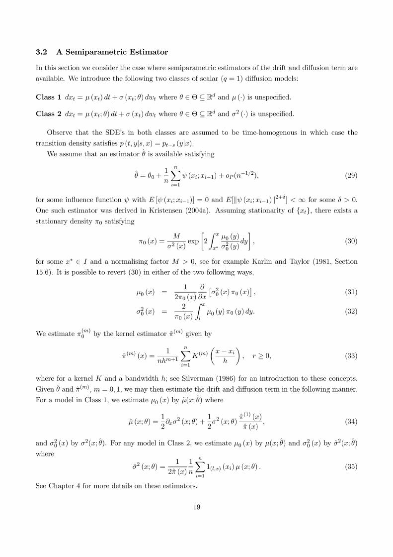
3.2 A Semiparametric Estimator

In this section we consider the case where semiparametric estimators of the drift and diffusion term are

available. We introduce the following two classes of scalar (q = 1) diffusion models:

Class 1 dxt = µ (xt) dt+ σ (xt; θ) dwt where θ ∈ Θ ⊆ Rd and µ (·) is unspecified.

Class 2 dxt = µ (xt; θ)dt+ σ (xt) dwt where θ ∈ Θ ⊆ Rd and σ2 (·) is unspecified.

Observe that the SDE’s in both classes are assumed to be time-homogenous in which case the

transition density satisfies p (t, y|s, x) = pt−s (y|x).We assume that an estimator θ is available satisfying

θ = θ0 +1

n

nXi=1

ψ (xi;xi−1) + oP (n−1/2), (29)

for some influence function ψ with E [ψ (xi;xi−1)] = 0 and E[kψ (xi;xi−1)k2+δ] < ∞ for some δ > 0.

One such estimator was derived in Kristensen (2004a). Assuming stationarity of xt, there exists astationary density π0 satisfying

π0 (x) =M

σ2 (x)exp

·2

Z x

x∗

µ0 (y)

σ20 (y)dy

¸, (30)

for some x∗ ∈ I and a normalising factor M > 0, see for example Karlin and Taylor (1981, Section

15.6). It is possible to revert (30) in either of the two following ways,

µ0 (x) =1

2π0 (x)

∂

∂x

£σ20 (x)π0 (x)

¤, (31)

σ20 (x) =2

π0 (x)

Z x

lµ0 (y)π0 (y)dy. (32)

We estimate π(m)0 by the kernel estimator π(m) given by

π(m) (x) =1

nhm+1

nXi=1

K(m)

µx− xih

¶, r ≥ 0, (33)

where for a kernel K and a bandwidth h; see Silverman (1986) for an introduction to these concepts.

Given θ and π(m), m = 0, 1, we may then estimate the drift and diffusion term in the following manner.

For a model in Class 1, we estimate µ0 (x) by µ(x; θ) where

µ (x; θ) =1

2∂xσ

2 (x; θ) +1

2σ2 (x; θ)

π(1) (x)

π (x), (34)

and σ20 (x) by σ2(x; θ). For any model in Class 2, we estimate µ0 (x) by µ(x; θ) and σ20 (x) by σ2(x; θ)

where

σ2 (x; θ) =1

2π (x)

1

n

nXi=1

1(l,x) (xi)µ (x; θ) . (35)

See Chapter 4 for more details on these estimators.

19

In Class 1, given consistency of θ, σ2(x; θ) is a pointwise consistent estimator of σ2 (x) given smooth-

ness conditions of σ2 (x; θ) w.r.t. θ. This in turn yields consistency of µ(x; θ) in (34) by the delta method.

Similarly for Class 2. We note that in both cases the convergence rate of the nonparametric part is

slower than√n.

In the following, we will derive the asymptotics of u in each of the two classes. In order to do this

we need to establish consistency of the two nonparametric estimators in the function norms k·k0,4 andk·k1,4. For this to hold, we need to introduce trimming in order to control the tailbehaviour of π sincethis appears in the denominator of both estimators. To this end, we introduce a trimming function, T ,

which we require satisfies

T (x;π, a) =

(1, π (x) ≥ a

0, π (x) ≤ a/2, (36)

for a positive sequence a = a such that a→ 0. We impose further regularity conditions on the trimming

function:

T (ω) The function T (x;π, a) (i) satisfies (36), (ii) is ω times continuously differentiable in x with

∂ixT (x;π, a) bounded, i = 0, ..., ω, and (iii) continuously differentiable in a with a∂aT (x;π, a)

bounded.

In the following we shall write T (x;a) = T (x; π, a) and T0 (x;a) = T (x;π0, a). Given T , we redefine

µ in Class 1 as

µ (x) =

(1

2∂xσ

2³x; θ´+1

2σ2³x; θ´ π(1) (x)

π (x)

)T (x; a) . (37)

Similarly, we redefine σ2 in Class 2 as

σ2 (x) =n−1

Pni=1 1(l,x) (xi) µ (xi)

2π (x)T (x;a) . (38)

In order to establish sufficiently fast convergence of the nonparametric part in the appropriate functional

norm, we introduce the following class K (ω, λ) of higher-order, bias-reducing kernels, first proposed byParzen (1962):

K (ω, λ) The kernelK satisfiesRRK (x) dx = 1;

RR x

iK (x) dx = 0, for 0 ≤ i ≤ ω−1;RR |x|

ω |K (x)| dx <

∞; K(i) (x)→ 0 as |x|→∞, 0 ≤ i ≤ λ− 1;

supx∈R¯K(i) (x)

¯max (|x| , 1) <∞, 0 ≤ i ≤ λ+1; K(i) is absolutely integrable with Fourier transform

Ψi satisfyingRR (1 + |x|) supb≥1 |Ψi (bx)| dx <∞, 0 ≤ i ≤ λ.

We first derive the asymptotics for models in Class1. We assume the following:

SP.0 The sequence xi is stationary and β-mixing with geometrically decreasing mixing coefficients.

SP.1 The marginal density π0 is ω times continuously differentiable with bounded derivatives.

SP.2¡µ0, σ

20

¢∈ D.

SP.3 The estimator θ satisfies (29) with θ0 ∈ intΘ.

20

SP.4 The transition density pt exists for any t ≥ 0 such that the mapping y 7→ pt (y|x) is bounded,and continuously differentiable with bounded first derivative.

SP1.A The kernel K ∈ K (ω, 2) and the trimming function T ∈ T (2). The bandwidth h and the

trimming parameter a satisfies n−1/2ak−2h−2−k → 0 and ak−2hω−k → 0, k = 0, 1, as a, h→ 0.

SP1.B The bandwidth h and the trimming parameter a satisfies

1. n−1/4ak−2h−1−k → 0 and n1/4ak−2hω−k → 0, k = 0, 1, 2.

2.R Tt Pt,x

¡a/2 ≤ π0

¡X0s

¢≤ a

¢ds = o(n−4).

Theorem 6 (Class 1) Assume that (SP.0)-(SP.3) and (SP1.A) hold and ω ≥ 3. Then ku− u0k0,1 =oP (1). If additionally (SP.4) and (SP1.B) hold and ω ≥ 4, then

√n (u (t, x)− u0 (t, x))

d→ N (0, V (t, x)) ,

where

V (t, x) = var (ν (x1|x0; t, x)) + 2∞Xi=1

cov (ν (x1|x0; t, x) , ν (xi+1|xi; t, x))

and ν (xi|xi−1; t, x) is given in (46).

Next, we derive the asymptotics in Class 2. This is done under very much the same assumptions

as the ones assumed for Class 1. Only do we need to slightly change the conditions on the bandwidth

and trimming parameter:

SP2.A The kernel K ∈ K (ω, 1) and the trimming function T ∈ T (1). The bandwidth h and the

trimming parameter a satisfies n−1/2a−1h−1 → 0 and a−1hω → 0 as a, h→ 0.

SP2.B The bandwidth h and the trimming parameter a satisfies

1. n−1/4ak−2h−1−k → 0 and n1/4ak−2hω−k → 0, k = 0, 1.

2. a8R Tt Pt,x

¡a/2 ≤ π0

¡X0s

¢≤ a

¢ds = o(n−4).

Theorem 7 (Class 2) Assume that (SP.0)-(SP.3) and (SP2.A) hold and ω ≥ 2. Then ku− u0k0,1 =oP (1). If additionally (SP.4) and (SP2.B) hold and ω ≥ 3, then

√n (u (t, x)− u0 (t, x))

d→ N (0, V (t, x)) ,

where

V (t, x) = var (ν (xi|xi−1; t, x)) + 2∞Xi=1

cov (ν (x1|x0; t, x) , ν (xi+1|xi; t, x))

and νi (t, x) is given in (49).

21

Sufficient conditions for (SP.0) to hold can be found in Kristensen (2004a). (SP.1) holds if µ0 and

σ20 both are ω times continuously differentiable. Aït-Sahalia (2002) gives sufficient conditions for (SP.4)

to hold

For both classes of estimators, the asymptotic variance V (t, x) is of unknown form. One can use

bootstrap methods to obtain an approximation of the distribution of the estimator. Alternatively, one

can use an idea originating from Newey (1994a) to estimate the variance using the pathwise derivative.

We only present the variance estimator for Class 1; the Class 2 case is dealt with similarly. We define

V (t, x) = Ω0 (t, x) +MPi=1

wM,i(Ωi (t, x) + Ω>i (t, x)),

where wM,i = 1− [i/ (M + 1)], Ωi (t, x) = n−1Pn

j=i ωj (t, x) ω>j−i (t, x), ωj (t, x) = ν

(1)j (t, x)+ ν

(2)j (t, x),

and

ν(1)j (t, x) =

∂Γ(µ(·; θ, π + αKh (·− xj)), σ2(·; θ), ) (t, x)

∂α

¯¯α=0

,

ν(2)j (t, x) =

∂Γ(µ(·; θ, π), σ2(·; θ), ) (t, x)∂θ

¯θ=θ

ψ (xj |xj−1) .

The two functions can be calculated using numerical derivatives. This estimator should be consistent

as M →∞ and M/n1/8 → 0. We will not give a formal proof of this, and instead refer to Section 4.4.

3.3 A Nonparametric Estimator

In this section we shall consider fully nonparametric kernel estimators of µ and σ2 in the univariate case,

q = 1. Such estimators have been considered in a series of papers, see e.g. Florens-Zmirou (1993), Jiang

and Knight (1997), Stanton (1997), Bandi and Moloche (2001), Bandi and Phillips (2003). All these

papers consider a sampling scheme where the time distance between observations ∆ = ∆n → 0, as the

number of observations n→∞; this is the so-called in-fill assumption. This enables one to reconstructthe full sample path in any compact interval in the limit, and thereby extract enough information about

the infinitesimal conditional variance, σ2, for it to be estimable. However, to construct an estimator of

the infinitesimal mean, µ, it is necessary also to require that the length of the time interval in which

the process is observed, T →∞; this is the so-called long-span assumption. Bandi and Phillips (2003)obtain pointwise consistency and mixed asymptotic normality of the drift and diffusion estimators only

assuming recurrence of the process thereby allowing for certain forms of non-stationarity. We apply the

estimators proposed by Bandi and Phillips (2003). But it appears to be difficult to work under their

general assumption of recurrence since the convergence rates of the estimators in the general case is

path-dependent. This in particular makes it difficult to show consistency in a functional norm. So for

simplicity, we restrict our attention to diffusion processes having a stationary marginal density π.

We assume that we have observed xi, xi = xi∆ , in the interval£0, T

¤where T = n∆→∞. We

shall assume that xt takes values on the interval I ⊆ R, and that the process is stationary and mixing.As we shall see, the nonparametric estimator of µ used here only has

√T h =

√n∆h-convergence rate,

while the nonparametric estimator of σ2 exhibits faster√nh-convergence rate. This in turn will mean

22

that the drift estimator will be the dominating term when deriving the asymptotics of u. In particular,

the convergence rate of u is√T and not

√n.

Before we define our estimators, we first introduce m (x) ≡ µ (x)π (x) and s (x) ≡ σ2 (x)π (x) such

that

µ (x) =m (x)

π (x), σ2 (x) =

s (x)

π (x).

We then construct kernel estimators of π, m, and s,

π (x) = n−1nXi=1

Kh (xi − x) ,

m (x) = n−1nXi=1

Kh (xi − x)xi+1 − xi∆

,

s (x) = n−1nXi=1

Kh (xi − x)(xi+1 − xi)

2

∆.

As in the previous section, we need to control the tailbehaviour of π. So we introduce trimmed versions

of our estimators,

µ (x) = T (x;a)m (x)

π (x), σ2 (x) = T (x;a)

s (x)

π (x).

The basic conditions are almost the same as the ones assumed for the semiparametric estimators:

NP.0 xt is stationary and β-mixing with geometrically decreasing mixing coefficients.

NP.1 The kernel K ∈ K (ω, 1) and the trimming function T ∈ T (1).

NP.2 The marginal density π0 is ω times continuously differentiable with bounded derivatives.

NP.3¡µ0, σ

20

¢∈ D.

NP.4 The transition density pt exists for any t ≥ 0 such that the mapping y 7→ pt (y|x) is bounded,and continuously differentiable with bounded derivative.

NP.5A The bandwidth h and the trimming parameter a satisfies T−1/2a−2h−1 → 0, a−2hω → 0, and

T 1/2+δqlog2

¡T¢∆3/4 log

¡∆−1

¢1/4a−2h−2 → 0, as a, h→ 0.

NP.5B The bandwidth h and the trimming parameter a satisfies

1. T 3/4+δqlog2

¡T¢∆3/4 log

¡∆−1

¢1/4ak−2h−2−k → 0, T−1/4ak−2h−1−k → 0 and T 1/4ak−2hω−k →

0, k = 0, 1.

2.R Tt Pt,x

¡a/2 ≤ π0

¡X0s

¢≤ a

¢ds = o(n−4).

Applying results from Bosq (1998), we are able to show that π, m, and s are uniformly consistent on

I, and also supply convergence rates. Given these, it is then an easy task to show that the nonparametric

estimators of µ and σ2 converge in the k·k0,4-norm. This shows consistency. We are able to strengthenthis kµ− µ0k1,4 = oP

¡T−1/4

¢and

°°σ2 − σ20°°1,4= oP

¡T−1/4

¢. The pathwise derivative consists of two

23

parts, the first part being a functional of µ, ∇1Γ, and the second a functional of σ2, ∇2Γ. It can now beshown that ∇1Γ [µ− µ0] converges towards a normal distribution with speed

√T , while ∇2Γ

£σ2 − σ20

¤does so with speed

√n. Thus, the first term dominates the second one, implying that ∇1Γ [µ− µ0]

drives the asymptotic distribution.

Theorem 8 (Nonparametric) Assume that (NP.0)-(NP.3) together with (NP.5A) hold with ω ≥ 2.Then the nonparametric estimator u is consistent. If additionally (NP4) and (NP5.B) hold thenp

T (u (t, x)− u0 (t, x))d→ N (0, V (t, x)) ,

where

V (t, x) = E

"σ20 (xs)

d∗2µ (xs)π20 (xs)

µZ T

tpu (xs|x) du

¶2#,

with d∗1 given in (24).

We propose to estimate the variance by V (t, x) as given in the previous section, only we redefine

ν(1)j (t, x) and ν

(2)j (t, x) as

ν(1)j (t, x) =

∂Γ(µ(·; π + αKh (·− xj) , m), σ2(·; π, s), ) (t, x)

∂α

¯α=0

,

ν(2)j (t, x) =

∂Γ(µ(·; π, m+ α (xj+1 − xj)Kh (·− xj) /∆), σ2(·; π, s), ) (t, x)

∂α

¯α=0

.

The two functions can be calculated using numerical methods. This estimator should be consistent as

M →∞ and M/T 1/8 → 0. We will not give a formal proof of this.

Bandi and Moloche (2001) generalise the above nonparametric estimators of µ and σ2 to the mul-

tivariate case. In Jeffrey et al (2004), a kernel estimator of the volatility function in a class of Heath-

Jarrow-Morton models is proposed. Series estimator of µ and σ2 for a one-dimensional diffusion has

been proposed by Chen et al (2000a, b). We conjecture that similar results to the one given above can

be derived for these estimators. In particular, the curse of dimensionality will not be a problem in the

estimation of u; the dimension of the underlying diffusion process Xt will have no effect on the rateof convergence.

Jiang and Knight (1997) propose an alternative drift estimator that makes explicit use of the

assumption of stationarity of the process. Jiang (1998) examines the estimation of solutions to PDE’s

when their nonparametric estimators are plugged in. He claims that the estimated solution, u, converges

with√n-rate. We believe there is a mistake in his proof since his drift estimator only converges with

speed√T h3. Thus, the convergence of u should not be able to exceed

√T .

4 Applications

In this section, we return to the examples given in Section 2.1 and 2.2 and discuss how the results

derived in the previous section can be applied to these.

We discussed in Section 2.1 how LPDE’s can be used to characterise derivative prices. The results

given in the previous section can now ensures that option prices calculated using preliminary estimated

24

models of the underlying variables are consistent and asymptotically normally distributed in great

generality. In particular, this enables us to calculate standard errors of the estimated prices which gives

us a measure of the statistical accuracy of the prices and allows us to test the individual asset pricing

model.

Example 1 (continued). Under the physical measure P , assume that we have a parametric diffusion

model of (8),

dSt = µS (t, St; θ) dt+ σS (t, St; θ)dwSt , (39)

the dividend stream is zero, dt = 0, and the short-rate is assumed to be constant, rt = r > 0. We

assume that an estimator θ of θ is available; this may have been obtained using historical observations of

the stock prices, Si∆, i = 1, ..., n, and applying MLE, GMM or some other method. Defining xi = Si∆,

µ = µS , and σ = σS , Theorem 5 gives conditions under which any implied derivative price based on

this estimator will be asymptotically normally distributed.

In the stochastic volatility model, we also have to obtain an estimator of the market price for

volatility, λ. Assuming that this is a known function up to θ, λ (S, v) = λ (S, v; θ), the results carry

through given smoothness conditions on λ of the same type as imposed on µS (t, S; θ) and σ2S (t, S; θ).

The estimator of λ may have been obtained using other data than historical observations of the stock

price(s). This can also be accommodated for.

Example 2 (continued). We assume that we have observed the short rate at discrete points in time,

ri∆, i = 1, ..., n, and that it under P solves

drt = µ (rt) dt+ σ (rt; θ)dwt.

The semiparametric estimator considered in Section 3.2 is then used to estimate µ and σ2. Taking the

market price of risk, λ (r), for given/known, Theorem 6 gives us the asymptotic distribution of any

implied bond and interest rate derivative price.

We can also allow for an unknown market price for risk for which we have an estimator, λ. Since

λ (r) enters the drift function linearly, one can easily accommodate for this in our proofs. Defining

µλ = µ− λσ, we first obtain¯u (t, x)− u0 (t, x)−∇Γ[µλ − µλ0 , σ

2 − σ20] (t, x)¯≤ b (x, T ) (||µλ − µλ0 ||21,4 + ||σ2 − σ20||21,4),

where°°σ2 − σ20

°°1,4= oP (n

−1/4) and

||µλ − µλ0 ||1,4 ≤ ||µ− µ0||1,4 + λ||21,4σ − σ0||1,4 + kσ0k1,4 λ− λ0||1,4 = oP (n−1/4),

if ||λ− λ0||1,4 = oP (n−1/4). Next, due to the linearity of ∇1Γ,

∇Γ[µλ − µλ0 , σ2 − σ20] (t, x) = ∇1Γ[λσ − λ0σ0] (t, x) +∇1Γ[µ− µ0] (t, x)

+∇2Γ[σ2 − σ20] (t, x) .

The second and third term is treated in the proof of Theorem 6, while the first one requires a bit of

work: Observe that

λσ − λ0σ0 = σ0(λ− λ0) +λ0σ0

¡σ2 − σ20

¢+O(||σ2 − σ20||2 + ||λ− λ0||2),

25

such that

∇1Γ[λσ − λ0σ0] (t, x) = ∇1Γ[σ0(λ− λ0)] (t, x) +∇1Γ£λ0/σ0

¡σ2 − σ20

¢¤(t, x)

+O³||σ2 − σ20||20,2 + ||λ− λ0||20,2

´.

The term ∇1Γ[λ0/σ0(σ2−σ20)] can be treated as ∇2Γ[σ2−σ20], while ∇1Γ[σ0(λ−λ0)], will converge in

distribution in great generality.

Next we turn to the two examples given in Section 2.2 concerning the estimation of diffusion models.

We check for each of the two examples that under regularity conditions the proposed estimator will be

consistent and asymptotically normally distributed.

Example 4 (continued). We here give primitive conditions under which the estimator proposed by

Bibby and Sørensen (1995) is consistent and asymptotically normally distributed. For simplicity, we

only consider the univariate case (q = 1) and assume that b (x) = x, while α (x; θ) = α (x) is parameter

independent. We first set up a set of conditions:

C.4.1 There exists p ≥ 2 and constants c0, c1 > 0 such that

2µ (x; θ) kxk2p−1 + (p− 1)σ20 (x) kxk2(p−1) ≤ c0 − c1 kxk2p .

C.4.2 The drift and diffusion function,¡µ (·; θ) , σ2 (·; θ)

¢, in (18) belongs to D for any θ ∈ Θ.

C.4.3 The function α : R 7→R satisfies |α (x)| ≤ C³1 + kxkp/2

´.

C.4.4 The matrix H (θ) ≡ Eθ [g (X∆|X0; θ)] is positive definite.

It now follows from Theorem 2 and 3 that B (x; θ) is continuously differentiable in θ, and by (6)

|B (x; θ)| ≤ C (K,∆) (1 + |x|),¯B (x; θ)

¯≤ C (K,∆) (1 + |x|2). The first condition implies, c.f. Meyn

and Tweedie (1993), that Xt is stationary and ergodic (assuming it has been started at its invariantdistribution) with Eπ[|X0|2p] <∞. We have that

|g (y|x; θ)|2 ≤ C¡1 + kxkp

¢³|y|2 + |x|2

´, kg (y|x; θ)k ≤ C

³1 + kxkp/2

´³|y|2 + |x|2

´where

Eh¡1 + kX0kp

¢ ³|X∆|2 + |X0|2

´i≤ CE

h1 + kX0k2p

i1/2Eπ

h³|X∆|4 + |X0|4

´i1/2<∞.

By Law of Large Numbers and a central limit theorem for martingales, we now obtain that√n(θ − θ0)→d N

¡0,H−1 (θ0)V (θ0)H−1 (θ0)

¢(40)

where V (θ) = Eθ

hg (X∆|X0; θ) g (X∆|X0; θ)>

i.

Example 5 (continued). We here give conditions under which the least squares estimator of θ based on

observe option prices is consistent and asymptotically normally distributed,

θ = argminθ∈Θ

nXi=1

(Pi −Π (Xi, T ; θ))2 ,

where Xi = Xi∆. We assume that (C.4.1)-(C.4.2) hold and that

26

C.5.1 The pay-off function g : R 7→R is continuously differentiable and satisfies¯∂ixg (x)

¯≤ C

³1 + kxkp/2

´,

i = 0, 1.

C.5.2 The matrix H (θ) ≡ Eθ

hΠ (Xi, T ; θ) Π (Xi, T ; θ)

>iis positive definite.

C.5.3 The error sequence εi is independent of Xi, i.i.d. and with E [εi] = 0, σ2ε = E£ε2i¤<∞.

Under (C.4.1)-(C.4.2) and (C.5.1)-(C.5.2), we obtain by standard arguments that

√n(θ − θ0)→d N

¡0, σ2εH

−1 (θ0)¢. (41)

The assumptions in (C.5.3) on the errors can be weakened substantially.

5 Conclusion

We have investigated the properties of estimated solutions of a PDE given preliminary estimates of

the driving coefficients of the PDE. We gave general conditions under which the estimated solution

was consistent and asymptotically normally distributed, and checked that these were satisfied in three

leading examples.

We demonstrated that these results have widespread use both in finance and econometrics. In

particular, the results can be used when drawing inference on implied derivative prices given estimates

of the dynamics of the underlying asset. Also in the literature on estimation of discretely observed

diffusions are our results useful.

A Proofs

Proof of Theorem 1. We have that

|u (t, x)| ≤ Et,x [|b (XT )|] +Et,x

·Z T

t|c (s,Xs)| ds

¸≤ C (1 +Et,x [|XT |r]) +Et,x

·Z T

tC (1 +Et,x [|Xs|r]) ds

¸≤ C (1 + kxkr) ,

where we have used (6). We obtain that

∂u (t, x)

∂xi= Et,x

·exp

·−Z T

ta (u,Xu) du

¸½bx (XT )Y

(i)T − b (XT )

Z T

tax (s,Xs)Y

(i)s ds

+

Z T

tcx (s,Xs)Y

(i)s − c (s,Xs)

Z s

tax (u,Xu)Y

(i)u du

¾¸.

27

where Y (i)t is given in Lemma 11, such that |∂u (t, x) /∂xi| is bounded by

Et,x

·kbx (XT )k ||Y (i)T ||+ |b (XT )|

Z T

tkax (s,Xs)k ||Y (i)s ||ds

¸+Et,x

·Z T

t|cx (s,Xs)| ||Y (i)s ||+

Z s

tkax (u,Xu)k ||Y (i)u ||duds

¸≤ C

Ã1 +

µZ T

tEt,x

hkXsk2r

ids

¶1/2!Ã1 +

µZ T

tEt,x

h||Y (i)s ||2

ids

¶1/2!≤ C (1 + kxkq) ,

for any (t, x) ∈ [0, T ]×Rq, where we have used (6). The expression of ∂2u (t, x) /∂xi∂xj is not presented

for brevity; one may show that¯∂2u (t, x) /∂xi∂xj

¯≤ C (1 + kxkr) ,for any (t, x) ∈ [0, T ] × Rd. This

shows the first part of the theorem. We then easily realise that

kuk2,p ≤ C

µ1 +

Z T

0E£°°X0

t

°°pr¤¶ ≤ C (1 +E [kX∗kpr]) <∞,

for pr ≤ p∗.Proof of Theorem 2. We see that¯

Et,x

·b (XT ) exp

·−Z T

ta (u,Xu)du

¸− b

¡X0T

¢exp

·−Z T

ta¡u,X0

u

¢du

¸¸¯≤ C (1 + kxkr)

µZ T

tEt,x

h¯a (u,Xu)− a

¡u,X0

u

¢¯2idu

¶1/2+Et,x

£¯b (XT )− b

¡X0T

¢¯¤where, by Lemma 10,

Et,x

hka (u,Xu)− a (u,Xu)k2

i≤ C (u, x)

µZ u

tEt,x

h°°µ ¡v,X0v

¢− µ0

¡v,X0

v

¢°°4i dv+

Z u

tEt,x

h°°σ2 ¡v,X0v

¢− σ20

¡v,X0

v

¢°°4i dv¶1/2 ,with C (t, x) = Ct (1 + kxkr), and

Et,x

£¯b (XT )− b

¡X0T

¢¯¤≤ C (T, x)

µZ T

tEt,x

h°°µ ¡u,X0u

¢− µ0

¡u,X0

u

¢°°2i du+

Z T

tEt,x

h°°σ2 ¡u,X0u

¢− σ20

¡u,X0

u

¢°°2i du¶1/2 .Similarly, ¯

Et,x

·Z T

tc (s,Xs) exp

·−Z s

ta (u,Xu)du

¸ds

¸−Et,x

·Z T

tc¡s,X0

s

¢exp

·−Z s

ta¡u,X0

u

¢du

¸ds

¸¯≤ C (T, x)

µZ T

tEt,x

h°°µ ¡u,X0u

¢− µ0

¡u,X0

u

¢°°4i du+

Z T

tEt,x

h°°σ2 ¡u,X0u

¢− σ20

¡u,X0

u

¢°°4i du¶1/228

We conclude that

|u (t, x)− u0 (t, x)| ≤ C (T, x)

µZ T

tEt,x

h°°µ ¡u,X0u

¢− µ0

¡u,X0

u

¢°°4i du+

Z T

tEt,x

h°°σ2 ¡u,X0u

¢− σ20

¡u,X0

u

¢°°4i du¶1/4Taking expectations,

ku− u0k0,1 ≤ CT (1 +E [kX∗kq])nkµ− µ0k0,4 +

°°σ2 − σ20°°0,4

o.

Proof of Theorem 3. For any function f , we have°°°f (x)− f (x0)− f (1) (x0) (x− x0)°°° ≤ °°°f (2) (λx+ (1− λ)x0)

°°° kx− x0k2 ,

for some λ ∈ [0, 1]. Thus,¯Et,x

·b (XT ) exp

·−Z T

ta (u,Xu) du

¸¸−Et,x

·b¡X0T

¢exp

·−Z T

ta¡u,X0

u

¢du

¸¸−Et,x

·bx¡X0T

¢ £XT −X0

T

¤exp

·−Z T

ta¡u,X0

u

¢du

¸¸+Et,x

·b¡X0T

¢exp

·−Z T

ta¡s,X0

s

¢ds

¸µZ T

tax¡u,X0

s

¢ £Xs −X0

s

¤ds

¶¸¯|

≤ CTeCTh1 + kxk4r

i1/2(Et,x

·Z T

t

°°Xs −X0s

°°4 ds+¸1/2 +Et,x

h°°XT −X0T

°°4i1/2) ,

Also, ¯Et,x

·bx¡X0T

¢exp

·−Z T

ta¡u,X0

u

¢du

¸ £XT −X0

T −∇XT

¤¸¯≤ C (T, x)Et,x

h°°XT −X0T −∇XT

°°2i1/2and °°°°Et,x

·b¡X0T

¢exp

·−Z T

ta¡s,X0

s

¢ds

¸µZ T

tax¡u,X0

s

¢ £Xs −X0

s −∇Xs

¤ds

¶¸°°°°≤ C (T, x)Et,x

·µZ T

t

°°Xs −X0s −∇Xs

°°2 ds¶¸1/2Similarly, ¯

Et,x

·Z T

tc (s,Xs) exp

·−Z s

ta (u,Xu) du

¸ds

¸−Et,x

·Z T

tc¡s,X0

s

¢exp

·−Z s

ta¡u,X0

u

¢du

¸ds

¸−Et,x

·Z T

tcx¡s,X0

s

¢ £Xs −X0

s

¤exp

·−Z s

ta¡u,X0

u

¢du

¸ds

¸+Et,x

·Z T

tc¡s,X0

s

¢exp

·−Z s

ta¡u,X0

u

¢du

¸µZ s

tax¡u,X0

u

¢ £Xu −X0

u

¤du

¶ds

¸¯≤ C (T, x)Et,x

·Z T

t

°°Xs −X0s

°°4 ds¸1/2 ,29

and °°°°Et,x

·Z T

tcx¡s,X0

s

¢exp

·−Z s

ta¡u,X0

u

¢du

¸ £Xs −X0

s −∇Xs

¤ds

¸°°°°≤ C (T, x)Et,x

·Z T

t

°°XTs −X0s −∇Xs

°°2 ds¸1/2 .Combining these results we obtain

|u (t, x)− u0 (t, x)−∇Γ (t, x)|

≤ C (T, x)

(Et,x

·Z T

t

°°Xs −X0s

°°4 ds+¸1/2 +Et,x

h°°XT −X0T

°°4i1/2)

+C (T, x)Et,x

·µZ T

t

°°Xs −X0s −∇Xs

°°2 ds¶¸1/2 .An application of Lemma 9 and 12 then proves the claim.

The following inequalities yield the second part of the theorem: For any (dµ, dσ) ∈ D,¯Et,x

·bx¡X0T

¢∇XT

£dµ, dσ2

¤exp

·−Z T

ta¡u,X0

u

¢du

¸¸¯≤ Et,x

h°°bx ¡X0T

¢°°2i1/2Et,x

h°°∇XT

£dµ, dσ2

¤°°2i1/2 ,¯Et,x

·b¡X0T

¢exp

·−Z T

ta¡s,X0

s

¢ds

¸µZ T

tax¡u,X0

s

¢∇Xsds

¶¸¯≤ Et,x

·°°bx ¡X0T

¢°°2 Z T

tax¡u,X0

s

¢2ds

¸1/2Et,x

·Z T

t

°°∇Xs

£µ, σ2

¤°°2 ds¸1/2 ,¯Et,x

·Z T

tcx¡s,X0

s

¢∇Xs exp

·−Z s

ta¡u,X0

u

¢du

¸ds

¸¯≤ Et,x

·Z T

t

°°cx ¡s,X0s

¢°°2 ds¸1/2Et,x

·Z T

t

°°∇Xs

£dµ, dσ2

¤°°2 ds¸1/2 ,and ¯

Et,x

·Z T

tc¡s,X0

s

¢exp

·−Z s

ta¡u,X0

u

¢du

¸µZ s

tax¡u,X0

u

¢∇Xudu

¶ds

¸¯≤ Et,x

·Z T

t

°°c ¡s,X0s

¢°°2 Z s

ta2x¡u,X0

u

¢duds

¸Et,x

·Z T

t

°°∇Xs

£dµ, dσ2

¤°°2 ds¸1/2where

Et,x

h°°∇Xs

£dµ, dσ2

¤°°2i ≤ Z T

tEt,x

h°°dµ ¡X0u

¢°°2i du+ Z T

tEt,x

h°°dσ2 ¡X0u

¢°°2i du=

°°¡dµ, dσ2¢°°20,2

.

for all s ∈ [t, T ], by Lemma 12. We conclude that¡dµ, dσ2

¢7→ ∇Γ

£dµ, dσ2

¤is a linear, continuous

functional.

30

Proof of Theorem 6. Under the (SP.0)-(SP.3) and (SP1.A), it follows from Lemma 13 that

kµ− µ0k0,4 = oP (1), and kσ − σ0k0,4 = oP (1). The consistency part now follows from the first part

of Theorem 4. To prove asymptotic normality, we first observe from Lemma 13, that kµ− µ0k21,4 =oP (n

−1/2), and°°σ2 − σ20

°°21,4= oP (n

−1/2). Thus, the asymptotic distribution of u is determined by∇Γ as given in (19). We linearise µ and σ2 w.r.t. π, π(1) and θ: Define ∇µ0 = T∇πµ0 +∇θµ0 where

∇πµ0£dπ, dπ(1)

¤= ∇0µ0 [dπ] +∇1µ0

£dπ(1)

¤, and

∇0µ0 [dπ] = −12σ20 (x)

π(1)0 (x)

π20 (x)dπ (x) , ∇1µ0

hdπ(1)

i=1

2σ20 (x)

dπ(1) (x)

π0 (x),

∇θµ0 [dθ] = µ0 (x) dθ, µ0 (x) =1

2∂xσ

20 (x) +

1

2σ20 (x)

π(1)0 (x)

π0 (x)

and ∇σ20 [dθ] = ∇θσ20 [dθ] = σ20 (x) dθ, where σ

20 (x) = ∂θσ

2 (x; θ0). We observe from Lemma 14 that

||µ(·; θ)− µ0 −∇µ0[π − π0, θ − θ0]||0,2 = oP (n−1/2),

and

||σ2³·; θ´− σ20 −∇σ20[θ − θ0]||0,2 = oP (n

−1/2),

under (SP1.B). Since ∇Γ is linear,

∇Γ (t, x)£µ− µ0, σ

2 − σ20¤= ∇Γ (t, x)

£µ− µ0 −∇µ0, σ2 − σ20 −∇σ20

¤+∇Γ (t, x)

£∇µ0,∇σ20

¤,

where, by the continuity of ∇Γ, c.f. Theorem 3,

∇Γ (t, x)£µ− µ0 −∇µ0, σ2 − σ20 −∇σ20

¤≤ C||µ(·; θ)− µ0 −∇µ0[π − π0, θ − θ0]||0,2

+C||σ2¡X0s

¢− σ20

¡X0s

¢− σ2

¡X0s

¢(θ − θ0)||0,2

= oP (n−1/2).

By Riesz’s Representation Theorem,

∇Γ (t, x)£∇µ0,∇σ20

¤=

Z T

tEt,x

£d∗1¡X0u

¢∇0µ0

¡X0u

¢¤ds+

Z T

tEt,x

£d∗1¡X0u

¢∇1µ0

¡X0u

¢¤ds

+

Z T

tEt,x

£d∗1¡X0u

¢∇θµ0

¡X0u

¢¤ds+

Z T

tEt,x

£d∗1¡X0u

¢∇σ20

¡X0u

¢¤ds

for some d∗ = (d∗1, d∗2) ∈ D. Each of the four terms in the above expression will make up a part of theinfluence function for ∇Γ: First,Z T

tEt,x

£d∗1¡X0u

¢∇0µ0

¡X0u

¢[π]¤ds

= − 12n

nXi=1

Z T

t

ZT (y; a)d∗1 (y)σ

20 (y)

π(1)0 (y)

π20 (y)pu−t (y|x)

1

hK

µy − xih

¶dydu

=1

n

nXi=1

T (xi; a) ν1 (xi; t, x) +OP

¡a−1hω−1

¢.

31

where

ν1 (y; t, x) = −1

2d∗1 (y)σ

20 (y)

π(1)0 (y)

π20 (y)

Z T

tps−t (y|x) ds. (42)

The last equality follows from the fact that for any m times continuously differentiable function with

g(i) bounded, 0 ≤ i ≤ m,Zg (z)Kh (z − y)dz =

Zg (y + hz)K (z) dz

=

Z ng (y) + g(1) (y)hz + ...+ g(m) (z)hmzm

oK (z)dz

= g (y) + hmZ

gm (z) zmK (z)dz,

for some z ∈ [y, y + hz]. The result is then obtained by applying this with g = T ν1 and m = ω−1 suchthat g(m) =

Pmi=0 T

(i)ν(m−i)1 . The boundedness condition holds since T (i) (x; a) = 0, 1 ≤ i ≤ ω − 1, for

x outside a compact interval, while π0 (y)¯ν(ω−1)1 (y; t, x)

¯= O (1) such that T (y;a)

¯ν(ω−1)1 (y; t, x)

¯=

O¡a−1

¢. By the same arguments,Z T

tEt,x

hT¡X0s ; a¢d1¡X0s

¢∇1µ

¡X0s

¢ hπ(1)

iids =

1

n

nXi=1

T (xi; a) ν2 (xi; t, x) +OP

¡a−1hω−1

¢,

where

ν2 (y; t, x) = −1

2

∂

∂y

·d1 (y)σ

20 (y)

π0 (y)

½Z T

tps (y|x) ds

¾¸. (43)

The last two terms are easily dealt with sinceZ T

tEt,x

hd1¡X0s

¢µ¡X0s

¢(θ − θ0)

ids =

1

n

nXi=1

ν3 (xi|xi−1; t, x) + oP (n−1/2),

Et,x

hd2¡X0s

¢σ¡X0s

¢(θ − θ0)

ids =

1

n

nXi=1

ν4 (xi|xi−1; t, x) + oP (n−1/2),

where

ν(3) (xi|xi−1; t, x) =

½Z T

tEt,x

£d1¡X0s

¢µ0¡X0s

¢¤ds

¾ψ (xi|xi−1) , (44)

ν(4) (xi|xi−1; t, x) =

½Z T

tEt,x

£d2¡X0s

¢σ0¡X0s

¢¤ds

¾ψ (xi|xi−1) . (45)

All together, ∇Γ (t, x) = 1n

Pni=1 ν (xi|xi−1; t, x) + oP (n

−1/2) with

ν (xi|xi−1; t, x) =2X

k=1

νk (xi; t, x) +4X

k=3

νk (xi|xi−1; t, x) . (46)

Proof of Theorem 7. Under (SP2.A), kµ− µ0k0,4 = oP (1), and°°σ2 − σ20

°°0,4

= oP (1) by

Lemma 13 which gives us consistency. From Lemma 13, we obtain kµ− µ0k21,4 = oP (n−1/2), and

32

kσ − σ0k21,4 = oP (n−1/2) under (SP2.1)-(SP2.4) and (SP2.B). We linearise µ and σ w.r.t. π and θ:

Define ∇σ20 [dπ, dθ] = T∇πσ20 [dπ] +∇θσ

20 [dθ], where

∇πσ20 [dπ] = − dπ (x)

2π20 (x)

Z x

lµ0 (y)π0 (y)dy,

∇σ20 [dθ] = σ20 (x) dθ, σ20 (x) =1

2π0 (x)

Z x

lµ0 (y)dπ (y)dy,

and ∇µ0 [dθ] = ∇θµ0 [dθ] = µ0 (x) dθ, where µ0 (x) = ∂θµ (x; θ0). By standard Taylor expansions,

||µ(·; θ)− µ0 −∇µ0[θ − θ0]||1,4 = oP (n−1/2),

while by Lemma 14,

||σ2 − σ20 −∇σ20[π − π0, θ − θ0]|1,4 = oP (n−1/2),

under (SP2.B). Thus, by linearity and continuity of ∇Γ,

∇Γ (t, x)£µ− µ0, σ

2 − σ20¤=

Z T

tEt,x

£d∗1¡X0s

¢µ¡X0s

¢¤ds(θ − θ0)

+

Z T

tEt,x

£d∗2¡X0s

¢σ¡X0s

¢¤ds(θ − θ0)

+

Z T

tEt,x

£d∗2¡X0s

¢∇πσ

2¡X0s

¢[π − π0]

¤ds

+oP (n−1/2),

where d∗ is given by the Riesz Representation Theorem. Proceeding as in the proof of Theorem 6, we

obtain Z T

tEt,x

£d∗2¡X0s

¢∇πσ

2¡X0s

¢[π]¤ds =

1

n

nXi=1

ν1 (xi; t, x) + oP (n−1/2)

where

ν2 (y; t, x) = d∗2 (y)1

2π20 (y)

Z y

lµ0 (y)π0 (y)dy

Z T

tps (y|x)ds. (47)

The derivatives w.r.t. θ have the following influence function,

ν2 (y|z; t, x) =½Z T

tEt,x

£d∗1¡X0s

¢µ¡X0s

¢¤ds+

Z T

tEt,x

£d∗2¡X0s

¢σ¡X0s

¢¤ds

¾ψ (z; y) (48)

In total, ∇u (t, x) = 1n

Pni=1 ν (xi|xi−1; t, x) + oP

¡n−1/2

¢, where

ν (xi|xi−1; t, x) = ν1 (xi; t, x) + ν2 (xi|xi−1; t, x) (49)

Proof of Theorem 8. Under (NP.1)-(NP.4) and (NP.6a), µ and σ2 are consistent on I in the

k·k0,4-norm, c.f. Lemma 15. This proves consistency of u.To derive the asymptotic distribution of u, we proceed as in the previous two proofs. Apply-

ing Lemma 16, kµ− µ0k21,4 = oP¡T−1/2

¢, and

°°σ2 − σ20°°21,4= oP (n

−1/2). So as before, the asymp-totic distribution of u is determined by ∇Γ

£dµ, dσ2

¤as given in (19). We define ∇µ0 (x) [dm, dπ] =

33

T ∇mµ0 (x) [dm] +∇πµ0 (x) [dπ] and ∇σ20 (x) [ds, dπ] = T©∇sσ

20 (x) [dτ ] +∇πσ

20 (x) [dπ]

ªwhere

∇mµ0 (x) [dm] =1

π0 (x)dm (x) , ∇πµ0 (x) [dπ] = −

m0 (x)

π20 (x)dπ (x) (50)

∇sσ20 (x) [dτ ] =

1

π0 (x)ds (x) , ∇πσ

20 (x) [dπ] = −

s0 (x)

π20 (x)dπ (x) . (51)

Applying Lemma 16 once more, it easily follows that

kµ− µ0 −∇µ0 [m−m0, π − π0]k0,2 = oP (T−1/2),°°σ2 − σ20 −∇σ20 [s− s0, π − π0]

°°0,2

= oP (n−1/2).

Thus, by linearity and continuity of ∇Γ together with Riesz’s Representation Theorem,

∇Γ (t, x)£µ− µ0, σ

2 − σ20¤

=

Z T

tEt,x

£d∗1¡X0u

¢∇µ0

¡X0u

¢[m−m0, π − π0]

¤du

+

Z T

tEt,x

£d∗2¡X0u

¢∇σ20

¡X0u

¢[s− s0, π − π0]

¤du+ oP (T

−1/2).

We now show that this expression converges towards the claimed distribution:Z T

tEt,x

hT¡X0u;a¢d∗1¡X0u

¢∇mµ0

¡X0u

¢[m]idu

= n−1nXi=1

T (xi; a)xi+1 − xi∆

d∗1 (xi)1

π0 (xi)

Z T

tpu (xi|x)du+ oP (T

−1/2);

Z T

tEt,x

hT¡X0u; a¢d∗1¡X0u

¢∇πµ0

¡X0u

¢[π]idu

= −n−1nXi=1

T (xi; a)d∗1 (xi)

µ0 (xi)

π0 (xi)

Z T

tpu (xi|x) du+ oP (T

−1/2);

Z T

tEt,x

hT¡X0u; a¢d∗2¡X0u

¢∇σ20

¡X0u

¢[s]idu

= n−1nXi=1

T (xi;a)(xi+1 − xi)

2

∆

d∗2 (xi)π0 (xi)

Z T

tpu (xi|x) du+ oP (n

−1/2);

Z T

tEt,x

hT¡X0u;a¢d∗2¡X0u

¢∇σ20

¡X0u

¢[π]idu

= −n−1nXi=1

T (xi;a)d∗2 (xi)σ20 (xi)

π0 (xi)

Z T

tpu (xi|x)du+ oP

³n−1/2

´;

In both cases, the trimming is asymptotically negligible so in total,

∇Γ (t, x)£µ− µ0, σ

2 − σ20¤= n−1

nXi=1

½xi+1 − xi∆

− µ0 (xi)

¾d∗1 (xi)

+n−1nXi=1

((xi+1 − xi)

2

∆− σ20 (xi)

)d∗2 (xi) + oP (n

−1/2).

34

where

d∗i (y; t, x) = d∗i (y)1

π0 (y)

Z T

tpu (y|x)du.

Using same arguments as employed in the proof of Lemma 15,√∆√n

nXi=1

d∗1 (xi)½xi+1 − xi∆

− µ (xi)

¾=

1√T

Z T

0d∗1 (xs)σ (xs)dWs + oP (1) ,

√∆√n

nXi=1

d∗2 (xi)

((xi+1 − xi)

2

∆− σ20 (xi)

)= oP (1) .

Thus, pT∇Γ (t, x)

£µ− µ0, σ

2 − σ20¤=

1√T

Z T

0σ0 (xs) d

∗1 (xs; t, x)dWs + oP (1)

where the leading term weakly converges towards a normal distribution with mean zero and variance

V (x, t) = E£σ20 (x0) d

21 (x0; t, x)

¤.

B Auxiliary Lemmas

Lemma 9 For any¡µ, σ2

¢∈ D,

Es

h°°Xt −X0t

°°2i ≤ °°Xs −X0s

°°2 + 6Z T

sEs

h°°µ ¡X0u

¢− µ0

¡X0u

¢°°2i du+6

Z T

sEs

h°°σ2 ¡u,X0u

¢− σ20

¡u,X0

u

¢°°2i dufor s ≤ t ≤ T .

Lemma 10 For any¡µ, σ2

¢∈ D,

1. For any integer p ≥ 1, there exists constant C (p) such that

Es

h°°Xt −X0t

°°2pi≤

°°Xs −X0s

°°2p +C (m)

Z T

sEs

h°°µ ¡u,X0u

¢− µ0

¡u,X0

u

¢°°2pi du+C (m)

Z T

sEs

h°°σ ¡u,X0u

¢− σ0

¡u,X0

u

¢°°2pi du2. If f : [0, T ]×Rq 7→ R satisfies kf (t, x)− f (t, y)k ≤ C (1 + kxkp + kykp) (kx− yk) then

Ex,s

£°°f (t,Xt)− f¡t,X0

t

¢°°¤≤ C (t, x)

µZ t

sEx,s

h°°µ ¡u,X0u

¢− µ0

¡u,X0

u

¢°°2i duZ T

sEx,s

h°°σ2 ¡u,X0u

¢− σ20

¡u,X0

u

¢°°2i du¶1/2 ,where C (t, x) = Ct (1 + kxpk).

35

Lemma 11 For any¡µ, σ2

¢∈ D, the Rq-valued diffusion process

dY(i)t = µ(1) (t,Xs,x

t )Y(i)t dt+ Y

(i)t σ(1) (t,Xs,x

t )dWt, Y (i)s = ei, (52)

where ei = eij with eij = 0 for i 6= j and eii = 1, exists and Y(i)t = ∂Xs,x

t /∂xi in the L2-sense.

If furthermore µ and σ2 are twice continuously differentiable and satisfy

k∂αxµ (t, x)k+ k∂αxσ (t, x)k ≤ C (1 + kxk) ,

for |α| = 2 then Y(i,j)t = ∂2Xs,x

t /∂xi∂xj also exists in the L2-sense.

Lemma 12 For any¡µ, σ2

¢∈ D:

1. the process ∇1Xt given by

d∇1Xt =ndµ¡t,X0

t

¢+ µ

(1)0

¡t,X0

t

¢∇1Xt

odt+ σ

(1)0

¡t,X0

t

¢∇1XtdWt, (53)

and

d∇2Xt = µ(1)0

¡t,X0

t

¢∇2Xtdt+

½1

2σ−10

¡t,X0

t

¢dσ2

¡t,X0

t

¢+ σ

(1)0

¡t,X0

t

¢∇2Xt

¾dWt, (54)

with dµ = µ− µ0 , satisfies

Es

h°°Xt −X0t −∇Xt

°°2i≤

°°Xs −X0s

°°2 + X|α|≤1

Z t

sEs

h°°∂αxµ ¡u,X0u

¢− ∂αxµ0

¡u,X0

u

¢°°4i du (55)

where Xt solves SDE¡µ, σ20

¢and

Es

hk∇Xtk2

i≤Z t

sEs

h°°µ ¡u,X0u

¢− µ0

¡u,X0

u

¢°°2i du. (56)

2. The process ∇2Xt given in (54) with dσ2 = σ2 − σ20, satisfies

Es

h°°Xt −X0t −∇2Xt

°°2i (57)

≤°°Xs −X0

s

°°2 + σ−2X|α|≤1

Z t

sEs

h°°∂αxσ2 ¡u,X0u

¢− ∂αxσ

20

¡u,X0

u

¢°°4i duwhere Xt solves SDE

¡µ0, σ

2¢and

Es

hk∇2Xtk2

i≤ σ−2

Z t

sEs

h°°σ2 ¡u,X0u

¢− σ20

¡u,X0

u

¢°°2i du. (58)

36

B.1 The Semiparametric Estimator

Lemma 13 Under (SP.0)-(SP.3) and (SP1.A) [(SP2.A)], the estimators for (µ, σ) in Class 1 [2] satisfy

kµ− µ0k0,4 = oP (1) ,°°σ2 − σ20

°°0,4= oP (1) .

If additionally (SP1.B) [(SP2.B)] then

kµ− µ0k1,4 = oP³n−1/4

´,°°σ2 − σ20

°°1,4= oP

³n−1/4

´.

Proof. In Class 1, the convergence of the diffusion estimator follows by the arguments used in theparametric case. For the drift estimator, by Kristensen (2004a),

||µ(i) (·; θ)− Tµ(i)0 (·; θ) ||∞ ≤ C

i+1Xk=0

ak−2−i||π(k) − π(k)0 ||∞,

and

||π(k) − π(k)0 ||∞ = OP

³n−1/2h−1−k

´+OP

³hω−k

´. (59)

Furthermore, µ(i)0 (x)− µ(i)0 (x) = a∂aT (x; a)µ

(i)0 (x), a ∈ [0, a], such thatZ T

tEt,x

h||µ(i)0

¡X0s

¢− µ

(i)0

¡X0s

¢||4ids

≤ a4µZ T

tEt,x

h|∂aT (x; a) |8

ids

¶1/2µZ T

tEt,x

h||µ(i)0

¡X0s

¢||8ids

¶1/2,

whereR Tt Et,x

h||µ(i)0

¡X0s

¢||8ids <∞. Under (SP1.A), we obtain that a

³R Tt Et,x

h|∂aT (x; a) |8

ids´1/8

=

oP (1). Under (SP1.B), it is oP¡n−1/4

¢.

The result for σ2 follows along the same lines, again using the results obtained in Kristensen (2004a).

Lemma 14 Under (SP.0)-(SP.3) and (SP1.A-B), the estimators for (µ, σ) in Class 1 satisfy uniformlyin θ ∈ Θ,

||µ− µ0 −∇πµ[π − π0]−∇θµ[θ − θ0]||0,2 = oP (n−1/2),

||σ2 − σ20 −∇θσ2[θ − θ0]||0,2 = oP (n

−1/2).

Under (SP.0)-(SP.3) and (SP2.A-B), the estimators for (µ, σ) in Class 2 satisfy uniformly in θ ∈ Θ,

||µ− µ0 −∇θµ[θ − θ0]||1,4 = oP (n−1/2),

||σ2 − σ20 −∇πσ2[π − π0]−∇θσ

2[θ − θ0]||1,4 = oP (n−1/2).

Proof. The result for the diffusion estimator in Class 1 is proved by the same arguments as the onesapplied in the parametric case. For the drift estimator we have

µ(i)(x; θ) = µ(i) (x; θ0) + ∂θµ(i)¡x; θ¢(θ − θ0),

37

and, by the results of Kristensen (2004a),

||µ(i) (·; θ0)− µ(i)0 (·; θ0)−∇πµ

(i) (·; θ0) [π − π0] ||∞ ≤ Ck+1Xi=0

ai−k−3n ||π(i) − π(i)0 ||2∞,

where ∇πµ(i) is the pathwise derivative w.r.t. π. The convergence of the RHS is given in (59). Using

the same arguments as in the previous proof,Z T

tEt,x

h|µ(i)

¡X0s ; θ0

¢− µ(i)

¡X0s ; θ0

¢|4ids = oP

¡n−2

¢,

and Z T

tEt,x

h|∇µ(i)0 (x; θ0) [π − π0]−∇µ(i) (x; θ0) [π − π0] |4

ids = oP

¡n−2

¢,

under (SP1.B) for i = 0, 1. Also,

||∂θµ(i)¡x; θ¢− ∂θµ

(i) (x; θ0) || ≤ ||∂θµ(i)¡x; θ¢− ∂θµ

(i)¡x; θ¢||+ ||∂2θµ(i)

¡x; θ¢||||θ − θ0||

||∂ixσ2 − ∂ixσ20 − ∂ixσ

20(θ − θ0)|| ≤

°°∂ixσ2 ¡x; θ¢°° ||θ − θ0||2 ≤ ||∂ixσ2(x) ||||θ − θ0||2,

Given the assumptions, we see that the terms on the the right hand side of the above inequalities are

oP (n−1/2).The results for Class 2 follow along the same lines applying results of Kristensen (2004a).

B.2 The Nonparametric Estimator

Lemma 15 Under (NP.0 )-(NP.4 ),

supx∈I

¯π(k) (x)− π

(k)0 (x)

¯= OP (An,Th

−2k) +OP (T−1/2h−1−2k) +OP

³hω−k

´,

supx∈I

¯m(k) (x)−m

(k)0 (x)

¯= OP (An,Th

−2k) +OP (T−1/2h−1−2k) +OP

³hω−k

´,

supx∈I

¯s(k) (x)− s

(k)0 (x)

¯= OP (An,Th

−2k) +OP (T−1/2h−1−2k) +OP

³hω−k

´for k = 0, 1, where for some δ > 0,

An,T = T 1/2+δqlog2

¡T¢h−2∆3/4 log

¡∆−1

¢1/4.

Proof. Define π (x) = T−1R T0 Kh (xs − x)ds. We then first show that supx∈R |π (x)− π (x)| =

OP (An,T ). It holds that

E [|π (x)− π (x)|] ≤ 1

n

nXi=1

Z i∆

(i−1)∆E [|Kh (xi − x)−Kh (xs − x)|] ds

≤ C∆κn,Th2

where κn,T ≡ maxi sups∈[i∆,(i+1)∆] |xs − xi| = OP (∆1/2plog (∆−1)) by Levy’s modulus of continuity,

c.f. Karatzas and Shreve (1991, Theorem 9.25), and where the RHS does not depend on x. We then

38

use the same idea as in Bosq (1998, p. 50): Define Bn =©x : |x| ≤ T γ

ª, for some γ > 0, and a covering

of Bn,

Bi,n =

(x : |x− xi,n| ≤

T γ

Mn,T

), i = 1, ...,Mn,T .

We have for x ∈ Bi,n,

|π (x)− π (x)| ≤ |π (x)− π (xi,n)|+ |π (x)− π (xi,n)|+ |π (xi,n)− π (xi,n)| ,

where

|π (x)− π (xi,n)| ≤ CT γ

h2Mn,T

, |π (x)− π (xi,n)| ≤ CT γ

h2Mn,T

.

Thus,

A−1n,T sup|x|≤Tγ

|π (x)− π (x)| ≤ 2CA−1n,T T

γ

h2Mn,T

+A−1n,T maxi=1,...,Mn,T

|π (xi,n)− π (xi,n)|

with

P (A−1n,T maxi=1,...,Mn,T

|π (xi,n)− π (xi,n)| > ε) ≤Mn,TXi=1

P³A−1n,T |π (xi,n)− π (xi,n)| > ε

´≤ CMn,TA

−1n,T

∆κn,Tεh2

.

We choose Mn,T =hA−1n,T

T γh−2 log2¡T¢i+ 1, and using arguments similar to the ones in Bosq (1998,

p. 52), we then obtain supx∈R |π (x)− π (x)| = OP (An,T ) if

A−2n,T

T 1+δh−4 log2¡T¢∆κn,T = O (1)

for some δ > 0. Finally, applying the same arguments as Bosq (1998, Corollary 4.6), it holds

supx∈R

|π (x)− π0 (x)| = OP

³T−1/2h−1

´+OP (h

ω) .

The proof of that supx∈R¯π(1) (x)− π(1) (x)

¯= oP

¡T−1/4

¢is shown in a similar manner under the

condition that T 3+δ log2¡T¢2h−12∆3 log

¡∆−1

¢→ 0 for some δ > 0, while

supx∈R

|π(1) (x)− π(1)0 (x) | = OP (T

−1/2h−3) +OP

¡hω−1

¢.

The remaining two claims are shown along the same lines, see e.g. Bandi and Phillips (2003). We

briefly sketch the proofs. First we show that m (x) − m (x) = oP (T−1/4), where m (x) is given by

m (x) = T−1R T0 Kh (xs − x)µ (xs)ds. We have

xi+1 − xi∆

− µ (xi) = ∆−1Z (i+1)∆

i∆µ (xs)− µ (xi) ds+∆−1

Z (i+1)∆

i∆σ (xs) dWs, (60)

such that

1

n∆

nXi=1

Kh (xi − x)

Z (i+1)∆

i∆|µ (xs)− µ (xi)| ds ≤

κn,Tn

nXi=1

Kh (xi − x)¯µ(1 (xi + oP (1))

¯= OP

³κn,Th

´,

39

and ¯¯n−1

nXi=1

Kh (xi − x)µ (xi)− T−1Z T

0Kh (xs − x)µ (xs)ds

¯¯

≤ Kκn,Th2

T−1Z T

0|µ (xs)| ds+ K

κn,Th

T−1Z T

0

¯µ(1 (xs)

¯ds

= OP

³κn,Th2

´.

where the bound does not depend on x. Next,

E

"∆−1n−1

nXi=1

Z (i+1)∆

i∆σ (xs) [Kh (xi − x)−Kh (xs − x)] dws

#= 0,

and

E[|∆−1n−1nXi=1

Z (i+1)∆

i∆σ (xs) [Kh (xi − x)−Kh (xs − x)] dws|2] ≤ C

κ2n,T

h4T−1E

£σ2 (xs)

¤The process ST (x) = T−1

R T0 Kh

¡xs−xh

¢σ (xs) dws has mean zero and variance

var [ST (x)] =¡T h¢−1µ

σ2 (x)π (x)

ZK2 (z)dz + o (1)

¶.

Hence, ST (x) = OP (1/√T h). We may now extend this to uniform convergence. Finally, using same

arguments as in Bosq (1998, Section 4.3.1), we obtain that

supx∈R

|m (x)−m0 (x)| = OP

³T−1/2h−1/2

´+OP (h

ω) .

To prove supx∈R |s (x)− s0 (x)| = oP (T−1/4), we first apply Itô’s Lemma on (60) to obtain

(xi+1 − xi)2

∆− σ2 (xi) =

2

∆

Z (i+1)∆

i∆µ (xs) (xs − xi) ds+

1

∆

Z (i+1)∆

i∆σ2 (xs)− σ2 (xi)ds

+2

∆

Z (i+1)∆

i∆σ (xs) (xs − xi)dws,

and by using similar arguments as before,

2

∆n

nXi=1

Kh (xi − x)

Z (i+1)∆

i∆µ (xs) (xs − xi) ds = OP

Ãκ2n,T

h2

!,

2

∆n

nXi=1

Kh (xi − x)

Z (i+1)∆

i∆σ2 (xs)− σ2 (xi) ds = OP

³κn,Th2

´,

n−1nXi=1

Kh (xi − x)σ2 (xi)− T−1Z T

0Kh (xs − x)σ2 (xs) ds = OP

³κn,Th2

´,

and

T−1Z T

0Kh (xs − x)σ2 (xs)ds− σ2 (x) = OP (T

−1/2h−1/2) +OP (hω) .

40

The remaining variance term, Sn (x) = n−1∆−1Pn

i=1 si,n (x) with

si,n (x) = 2Kh (xi − x)

Z (i+1)∆

i∆σ (xs) (xs − xi)dws

defines a martingale, and we obtain

var [Sn (x)] =σ4 (x)π (x) + o (1)

nh+O

Ã∆1/2

plog (∆−1)h2

!.

Hence, Sn (x) = OP

³1/√nh´.

Lemma 16 1. Under (NP.0)-(NP.5A),

kµ− µ0k0,4 = oP (1) ,°°σ2 − σ20

°°0,4= oP (1) .

2. Under (NP.0)-(NP.5B),

kµ− µ0k1,4 = oP (T−1/4),

°°σ2 − σ20°°1,4= oP (n

−1/4),

kµ− µ0 −∇µk0,2 = oP (T−1/4),

°°σ2 − σ20 −∇σ2°°0,2= oP (n

−1/4),

where

∂xµ = T (x;a)

(m(1)

π− m

π

π(1)

π

), ∂xσ

2 = T (x; a)

(s(1)

π− s

π

π(1)

π

).

Proof. We have

Et,x

·Z T

t

¯µ(i)

¡X0s

¢− µ

(i)0

¡X0s

¢¯4ds

¸1/4≤ sup

x∈RT (x; a)

¯µ(i) (x)− µ

(i)0 (x)

¯+aE

·Z T

t|∂aT

¡X0s

¢;a|4

¯µ0¡X0s

¢¯4ds

¸1/4,

where

Et,x

·Z T

t|∂aT

¡X0s

¢;a|4|µ(i)0

¡X0s

¢|4ds

¸1/4≤ Et,x

·Z T

t|∂aT

¡X0s

¢;a|8ds

¸1/8Et,x

·Z T

t|µ(i)0

¡X0s

¢|8ds

¸1/8.

It holds that

supx∈R

T (x;a) |µ (x)− µ0 (x)| ≤ supx∈R

T (x; a)

¯m (x)

π (x)− m0 (x)

π0 (x)

¯≤ a−1 km−m0k∞ + a−2 kπ − π0k∞ ,

and

supx∈R

T (x; a)¯µ(1) (x)− µ

(1)0 (x)

¯≤ a−2 km−m0k∞ + a−1||m(1) −m

(1)0 ||∞ + a−3 kπ − π0k∞ + a−2||π(1) − π

(1)0 ||∞,

41

Using the rates of convergence established in Lemma 15, we obtain kµ− µ0k0,4 = oP (1) and kµ− µ0k1,4 =oP (T

−1/4) under (NP5.A) and (NP5.B) respectively.With ∇µ given in (50) it holds that

µ (x)− µ0 (x)−∇µ0 (x) [m−m0, π − π0]

=π (x)− π0 (x)

π (x)π0 (x)

·[m (x)−m0 (x)]−

m0 (x)

π0 (x)[π (x)− π0 (x)]

¸such that

|µ (x)− µ0 (x)−∇µ0 (x) [m−m0, π − π0]|

≤ T (x; a)1 + |m0 (x)|bπ (x)π0 (x)

n|m (x)−m0 (x)|2 + |π (x)− π0 (x)|2

o.

Thus, Z t

0

¯µ¡X0s

¢− µ0

¡X0s

¢−∇µ0

¡X0s

¢[m−m0, π − π0]

¯2ds

≤ C

Z t

0T¡X0s ;a¢Ã 1 + ¯m0

¡X0s

¢¯π (X0

s )π0 (X0s )

!2ds

1/2 ×µZ t

0

¯m¡X0s

¢−m0

¡X0s

¢¯2+¯π¡X0s

¢− π0

¡X0s

¢¯4ds

¶1/2where Z t

0T¡X0s ; a¢Ã 1 + ¯m0

¡X0s

¢¯π (X0

s )π0 (X0s )

!2ds ≤ a−2

Z t

01 +

¯µ0¡X0s

¢¯2ds.

References

Aït-Sahalia, Y. (1993) The Delta Method for Nonparametric Kernel Functionals. Working paper,

Princeton.

Aït-Sahalia, Y. (1996a) Nonparametric Pricing of Interest Rate Derivative Securities. Econometrica 64,

527-560.

Aït-Sahalia, Y. (2002) Maximum Likelihood Estimation of Discretely Sampled Diffusions: A Closed-

Form Approximation Approach. Econometrica 70, 223-262.

Aït-Sahalia, Y. & J. Duarte (2003) Nonparametric Option Pricing under Shape Restrictions. Journal

of Econometrics 116, 9-47.

Ames, W.F. (1992) Numerical Methods for Partial Differential Equations. Academic Press, San Diego.

Andrews, D.W.K. (1995) Nonparametric Kernel Estimation for Semiparametric Models. Econometric

Theory 11, 560-596.

42

Bandi, F.M. & G. Moloche (2001) On the Functional Estimation of Multivariate Diffusion Processes.

Working paper, MIT.

Bandi, F.M. & P.C.B. Phillips (2000) Accelerated Asymptotics for Diffusion Model Estimation. Working

paper, GSB, University of Chicago.

Bandi, F.M. & P.C.B. Phillips (2003) Fully Nonparametric Estimation of Scalar Diffusion Models.

Econometrica 71, 241-283.

Bibby, B. and M. Sørensen (1995) Martingale Estimating Functions for Discretely Observed Diffusion

Processes. Bernoulli 1, 17-39.

Bierens, H.J. (1987) Kernel Estimators of Regression Functions. In T.F. Bewley (ed.) Advances in

Econometrics: Fifth World Congress Vol. 1, 99-144. Cambridge: Cambridge University Press.

Björk, T. (1998) Arbitrage Theory in Continuous Time. Oxford: Oxford University Press.

Black, F. & M. Scholes (1973) The Pricing of Options and Corporate Liabilities. Journal of Political

Economy 81, 637-654.

Bosq, D. (1998) Nonparametric Statistics for Stochastic Processes. New York: Springer-Verlag.

Boyle, P.P. and A.L. Ananthanarayanan (1977) The Impact of Variance Estimation in Option Valuation

Models. Journal of Financial Economics 5, 375-388.

Broze, L., O. Scaillet & J.-M. Zakaïan (1998) Quasi-Indirect Inference for Diffusion Processes. Econo-

metric Theory 14, 161-186.

Carrasco, M., M. Chernov, J.-P. Florens & E. Ghysels (2002) Efficient Estimation of Jump Diffusions

and General Dynamic Models with a Continuum of Moment Conditions. Working paper, University

of Rochester.

Chacko, G. & L. Viceira (2003) Spectral GMM Estimation of Continuous-Time Processes. Journal of

Econometrics 116, 259-292.

Chen, X., L.P. Hansen & J. Scheinkman (2000a) Shape-preserving Estimation of Diffusions. Working

paper, University of Chicago.

Chen, X., L.P. Hansen & J. Scheinkman (2000b) Principal Components and the Long Run. Working

paper, University of Chicago.

Chow, P.-L., I.A. Ibragimov & R.Z. Khasminskii (1999) Statistical Approach to Some Ill-Posed Prob-

lems for Linear Partial Differential Equations. Probability Theory and Related Fields 113, 421-441.

Duffee, G.R. (2002) Term Premia and Interest Rate Forecasts in Affine Models. Journal of Finance 57,

405-443.

Duffie, D. (1996) Dynamic Asset Pricing Theory, 3rd edition. New Jersey: Princeton University Press.

43

Duffie, D. & R. Kan (1996) A Yield Curve Model of Interest Rates. Mathematical Finance, 6, 379-406.

Duffie, D. & K.J. Singleton (1993) Simulated Moments Estimation of Markov Models of Asset Prices.

Econometrica 61, 929-952.

Elerian, O., S. Chib, S. & N. Shephard (2001) Likelihood Inference for Discretely Observed Non-linear

Diffusions. Econometrica 69, 959-993.

Evans, L.C. (1998) Partial Differential Equations. Providence: American Mathematical Society.

Freidlin, M. (1985) Functional Integration and Partial Differential Equations. New Jersey: Princeton

University Press.

Friedman, A. (1964) Partial Differential Equations of Parabolic Type. New Jersey: Prentice-Hall.

Friedman, A. (1975) Stochastic Differential Equations and Applications, vol. 1. New York: Academic

Press.

Garcia, R., E. Ghysels and E. Renault (2004) The Econometrics of Option Pricing. Working paper

2004s-04, CIRANO. Forthcoming in Handbook of Financial Econometrics.

Gysels, E., A. Harvey & E. Renault (1996) Stochastic Volatility. In Handbook of Statistics, Vol. 14

(eds. Maddala, G. & C. Rao). Elsevier Science B.V.

Hall, P. (1992) The Bootstrap and Edgeworth Expansion. New York: Springer-Verlag.

Hall, P., S.N. Lahiri & J. Polzehl (1995) On Bandwidth Choice in Nonparametric Regression with Both

Short- and Long-Range Dependent Errors. Annals of Statistics 23, 1921-1936.

Hausman, J. & W. Newey (1995) Nonparametric Estimation of Exact Consumers Surplus and Dead-

weight Loss. Econometrica 63, 1445-1476.

Härdle, W., J.D. Hart, J.S. Marron & A.B. Tsybakov (1992) Bandwidth Choice for Average Derivative

Estimation. Journal of the American Statistical Association 87, 218-233.

Härdle, W., J.S. Marron & M.P. Wand (1990) Bandwidth Choice for Density Derivatives. Journal of

the Royal Statistical Society, Series B, 52, 223-232.

Heath, D.C., R.A. Jarrow & A. Morton (1992) Bond Pricing and the Term Structure of Interest Rates:

A New methodology for Contingent Claims Valuation. Econometrica 60, 77-105.

Heston, S.L. (1993) A Closed-Form Solution for Options with Stochastic Volatility with Applications

to Bond and Currency Options. Review of Financial Studies 6, 327-343

Ho, T.S.Y. & S.-B. Lee (1986) Term Structure Movements and Pricing Interest Rate Contingent Claims.

Journal of Finance 41, 1011-1029.

Horowitz, J. (2003) Bootstrap Methods for Markov Processes. Econometrica 71, 1049-1082.

Hull, J.C. (1997) Options, Futures and Other Derivatives. New Jersey: Prentice-Hall.

44

Hull, J.C. & A.D. White (1993) One-Factor Interest-Rate Models and the Valuation of Interest-Rate

Derivative Securities. Journal of Financial and Quantitative Analysis 28, 235-254.

Jeffrey, A., D. Kristensen, O. Linton, T. Nguyen & P.C.B. Phillips (2004) Nonparametric Estimation

of a Multifactor Heath-Jarrow-Morton Model: An Integrated Approach. Forthcoming in Journal

of Financial Econometrics.

Jiang, G (1998) Nonparametric Modeling of U.S. Interest Rate Term Structure Dynamics and Impli-

cations on the Prices of Derivative Securities. Journal of Financial and Quantitative Analysis 33,

465-497.

Jiang, G. & J. Knight (1997) A Nonparametric Approach to the Estimation of Diffusion Processes -

with an Application to a Short-term Interest Rate Model. Econometric Theory 13, 615-645.

Karatzas, I. & S.E. Shreve (1991) Brownian Motion and Stochastic Calculus, 2nd Edition. New York:

Springer Verlag.

Karlin, S. & H.M. Taylor (1981) A Second Course in Stochastic Processes. Academic Press.

Kloeden, P.E. & E. Platen (1999) Numerical Solution of Stochastic Differential Equations (2nd ed.).

Heidelberg: Springer-Verlag.

Kristensen, D. (2004a) Estimation in Two Classes of Semiparametric Diffusion Models. Working paper,

LSE.

Kristensen, D. (2004b) A Semiparametric Single-Factor Model for the Term Structure of Interest Rates.

Working paper, LSE.

Lo, A. (1986) Statistical Tests of Contingent-Claims Asset-Pricing Models. Journal of Financial Eco-

nomics 17, 143-173.

Lo, A. (1988) Maximum Likelihood Estimation of Generalized Itô Processes with Discretely Sampled

Data. Econometric Theory 4, 231-247.

Masry, E. (1996) Multivariate Local Polynomial Regression for Time Series: Uniform Strong Consis-

tency and Rates. Journal of Time Series Analysis 17, 571-599.

Merton, R.C. (1976) Option Pricing when Underlying Stock Returns Are Discontinuous. Journal of

Financial Economics 3, 125-144.

Meyn, S.P. & R.L. Tweedie (1993) Stability of Markovian processes III: Foster-Lyapunov Criteria for

Continuous-time Processes. Advances in Applied Probability 25, 518-548.

Ncube, M. & S. Satchell (1997) The Statistical Properties of the Black-Scholes Option Price. Mathe-

matical Finance 7, 287-305

Newey, W.K. (1994a) Kernel Estimation of Partial Means and a General Variance Estimator. Econo-

metric Theory 10, 233-253.

45

Newey, W.K., F. Hsieh & J. Robins (1992) Bias Corrected Semiparametric Estimation. Working paper,

MIT.

Newey, W.K., F. Hsieh & J. Robins (2004) Twicing Kernels and a Small Bias Property of Semipara-

metric Estimators. Econometrica 72, 947-962.

Newey, W.K. & K.D. West (1987) A Simple, Positive Semi-Definite, Heteroskedasticity and Autocor-

relation Consistent Covariance Matrix. Econometrica 55, 703-708.

Parzen, E. (1962) On Estimation of a Probability Density Function and Mode. Annals of Mathematical

Statistics 33, 1065-1076.

Pedersen, A.R. (1995) A New Approach to Maximum-Likelihood Estimation for Stochastic Differential

Equations Based on Discrete Observations. Scandinavian Journal of Statistics 22, 55-71.

Powell, J.L. & T.M. Stoker (1996) Optimal Bandwidth Choice for Density-Weighted Averages. Journal

of Econometrics 75, 291-316.

Robinson, P.M. & C. Velasco (1997) Autocorrelation-Robust Inference. In Robust Inference (eds. G.S.

Maddala & C.R. Rao), 267-298. Amsterdam: North-Holland.

Silverman, B.W. (1986) Density Estimation for Statistics and Data Analysis. Chapman and Hall.

Singleton, K. (2001) Estimation of Affine Pricing Models Using the Empirical Characteristic Function.

Journal of Econometrics 102, 111-141.

Stanton, R. (1997) A Nonparametric Model of Term Structure Dynamics and the Market Price of

Interest Rate Risk. Journal of Finance 52, 1973-2002.

Stoker, T.M. (1993) Smoothing Bias in Density Derivative Estimation. Journal of the American Sta-

tistical Association 88, 855-863.

Sundaresan, S.M. (2000) Continuous-Time Methods in Finance: A Review and an Assessment. Journal

of Finance 55, 1569-1622.

Vanhems, A. (2003) Nonparametric Study of Solutions of Differential Equations. Working paper, ESC

Toulouse.

Vasicek, O. (1977) An Equilibrium Characterization of the Term Structure. Journal of Financial Eco-

nomics 5, 177-188.

46