Identification and analysis of functional elements in -

Identification and analysis of functional elements in 1% of the human genome by the ENCODE pilot project This supplement contains methods of data generation and analysis as well as other technical information on the ENCODE project publication.

SUPPLEMENTARY INFORMATION

doi: 10.1038/nature05874

S1 ENCODE PROJECT TECHNICAL DETAILS ..............................................................................................3 S1.1 SUMMARY OF DATA SETS AND DATA ACCESS...............................................................................................3 S1.2 EXPERIMENTAL REPRODUCIBILITY AND CONFIRMATION .............................................................................13 S1.3 GENOME STRUCTURE CORRECTION.............................................................................................................13

S2 TRANSCRIPTION...........................................................................................................................................20 S2.1 TXFRAG AND GENOME TILING ARRAYS: DATA GENERATION AND ANALYSIS .............................................20 S2.2 5’-SPECIFIC CAP ANALYSIS GENE EXPRESSION (CAGE) ............................................................................28 S2.3 GENE IDENTIFICATION SIGNATURE – PAIRED END DITAGS (GIS-PET) .....................................................28 S2.4 THE GENCODE ANNOTATION....................................................................................................................30 S2.5 GENERATION OF TRANSCRIPT MAPS............................................................................................................35 S2.6 ANALYSIS OF PROTEIN CODING EVOLUTION.................................................................................................36 S2.7 EXPRESSION AND CONFIRMATION OF GENCODE TRANSCRIPTS AND UNUSUAL SPLICE VARIANTS .............40 S2.8 ANALYSIS OF UNANNOTATED TRANSFRAGS.................................................................................................41 S2.9 RACE AND GENOME TILING ARRAYS: DATA GENERATION AND ANALYSIS ................................................46 S2.10 PSEUDOGENE ANNOTATION.......................................................................................................................55 S2.11 NON-PROTEIN CODING RNAS ....................................................................................................................55 S2.12 GENOME REARRANGEMENTS OF ENCODE CELL LINES............................................................................58

S3 REGULATION OF TRANSCRIPTION ........................................................................................................61 S3.1 CHIP-CHIP AND CHIP-PET EXPERIMENTAL METHODOLOGY.......................................................................61 S3.2 STAGE DATA GENERATION METHODS.......................................................................................................73 S3.3 DNASEI SENSITIVITY AND HYPERSENSITIVITY: DATA GENERATION AND ANALYSIS ....................................74 S3.4 FAIRE DATA GENERATION METHODS.........................................................................................................76 S3.5 GENERATION AND CATEGORIZATION OF 5' END CLUSTERS...........................................................................76 S3.6 CHIP ENRICHMENT PROFILES FOR TSSS ......................................................................................................78 S3.7 SYMMETRICAL SIGNAL ANALYSIS...............................................................................................................92 S3.8 BAF ANALYSIS ...........................................................................................................................................93 S3.9 PREDICTION OF TSS ACTIVITY FROM CHROMATIN MODIFICATIONS .............................................................95 S3.10 RFBR IDENTIFICATION METHODS.............................................................................................................96 S3.11 DETECTION OF OVERREPRESENTED MOTIFS WITH AB INITIO METHODS .......................................................97 S3.12 SIGNIFICANCE OF RFBR ENRICHMENTS NEAR GENCODE TSSS ..............................................................99 S3.13 INTEGRATION APPROACHES TO GENERATE REGULATORY CLUSTER LISTS ...............................................100 S3.14 THE OVERLAP OF REGULATORY CLUSTERS WITH DIFFERENT TSS EVIDENCE CLASSES............................108 S3.15 CLONING PUTATIVE NOVEL PROMOTERS..................................................................................................109 S3.16 CONTROL FOR THE ASCERTAINMENT BIAS ..............................................................................................111 S3.17 CLASSIFICATION OF FUNCTIONAL ELEMENTS...........................................................................................112

S4 CHROMATIN ARCHITECTURE ...............................................................................................................116 S4.1 REPLICATION TIMING: DATA GENERATION AND ANALYSIS .......................................................................116 S4.2 CORRELATIONS BETWEEN CONTINUOUS CHROMATIN AND REPLICATION DATATYPES................................116 S4.3 CORRELATIONS OF HISTONE MODIFICATIONS WITH TR50 AT DISCRETE POINTS IN THE GENOME ...............119 S4.4 CHROMATIN:REPLICATION ENRICHMENT ANALYSIS ..................................................................................122 S4.5 HISTONE MODIFICATION PATTERNS OF DHSS............................................................................................123 S4.6 IDENTIFICATION AND ANALYSIS OF CORCS..............................................................................................124 S4.7 IDENTIFICATION OF HIGHER ORDER DOMAINS BY MULTI-TRACK HMM SEGMENTATION ...........................125

S5 EVOLUTION AND POPULATION GENETICS .......................................................................................125 S5.1 CONSERVATION OF REGULATORY ELEMENTS.............................................................................................125 S5.2 GENETIC VARIATION AND EXPERIMENTALLY-IDENTIFIED FUNCTIONAL ELEMENTS...................................127 S5.3 UNEXPLAINED CONSTRAINED SEQUENCES .................................................................................................131 S5.4 UNCONSTRAINED EXPERIMENTALLY-IDENTIFIED FUNCTIONAL ELEMENTS................................................133 S5.5 SENSITIVITY OF IDENTIFYING EVOLUTIONARY CONSERVED BASES ............................................................135

S6 REFERENCES ...............................................................................................................................................138

doi: 10.1038/nature05874 SUPPLEMENTARY INFORMATION

S1 ENCODE Project Technical Details

S1.1 Summary of Data Sets and Data Access In addition to the ENCODE data portal at the UCSC genome browser ( see Supplement S1.1.2 ) the ENCODE data are also being integrated with other genome browsers, such as Ensembl (http://www.ensembl.org/index.html) and NCBI Map Viewer (http://www.ncbi.nlm.nih.gov/mapview/). Archived raw microarray data and other numerical-valued data are available via the NCBI Gene Expression Omnibus (GEO) (http://www.ncbi.nlm.nih.gov/geo/) or the EBI ArrayExpress (http://www.ebi.ac.uk/arrayexpress/), and sequence-tag data have been submitted to EMBL/GenBank/DDBJ


S1.1.1 Datasets, acronyms, cell lines, references The table below lists the ENCODE datasets, acronyms used, cell lines, and references for each ENCODE dataset.

Dataset Description Source Cell lines Abbreviation Biological Samples

Biological Reps

Technical Rept

Array/data points size Total points

Accession Numbers

References

BU ORChID

ORChID (OH Radical Cleavage Intensity Database)

BU (Tullius)

Computational

CCI (Calculated cleavage intensity)

NA NA NA 30,000,000 30,000,000 Greenbaumet al1,

NHGRI DNaseI

DNaseI-Hypersensitive Sites

Duke/NHGRI

CD4, GM06990, Hela S3, HepG2

DHS 4 3 3 (different Dnase concentrations)

382,884 13,782,324 Crawford et al2

UNC FAIRE

Formaldehyde Assisted Isolation of Regulatory Elements

Univ N Carolina

2091Fib RFBR 1 cell line, 4 independent samples from independent cultures

4 0 384,000 1,536,000 GEO: GSE4886 Giresi et al3

UW DNaseI

UW QCP DNaseI

UW/ Regulome

GM06990, HELA, CACO2, SKNSH, CD4, HEPG2, HUH7, EryAdult, EryFetal, K562, PANC1, NHBE, CALU3, SAEC, HMEC,

DHS 16 Pooling 4-8 replicates

4-8 7.5 million qPCR reactions ~119,000 amplicons

7,620,000 GEO: GSE4334 Dorschner et al4


HRE

UW DNaseI

UW DNase-array

GM06990 DHS 1 2 N/A 384.000 768,000 Sabo et al5

GERP Cons

GERP conservation and conserved elements

Stanford (Sidow)

Computational

NA NA NA Cooper et al6

BinCons Cons

BinCons conservation and conserved elements

NHGRI (Margulies)

Computational

NA NA NA

Consens Elements

Consensus Constrained Elements

ENCODE MSA

Computational

MCS NA NA NA

DLESS Detection of Lineage-Specific Selection

UC Santa Cruz

Computational

NA NA NA

MAVID Alignment

MAVID Multiple Sequence Alignments

UC Berkeley (Pachter)

Computational

NA NA NA

MLAGAN Alignment

MLAGAN Multiple Sequence Alignments

Stanford (Batzoglou)

Computational

NA NA NA

PhastCons Cons

PhastCons Conservation and Conserved Elements

UC Santa Cruz

NA NA NA


SCONE Cons

SCONE Conservation and Conserved Elements

Harvard (Sunyaev)

Computational

NA NA NA

TBA Alignment

TBA Multiple Sequence Alignments

Penn State /NHGRI

Computational

NA NA NA

Uva DNA Rep

Temporal Profiling of DNA Replication

Univ Virginia

HeLa TR50 5 2 2 continous data set, 736,787 probes (25mer each) on affymetrix ENCODE array

14,735,740 E-MEXP-708 Jeon et al7

Uva DNA Rep Ori

DNA Replication Origins

Univ Virginia

TR50 minima 5 2 2 229 E-MEXP-708 Karnani et al8

BU First Exon

First Exon Activity

BU (Weng)

Computational

NA NA Ding & Cantor9 Ding & Cantor10 Halees et al11 Halees & Weng12

LI ChIP Ludwig Institute/UCSD ChIP/Chip

Ludwig Inst/UCSD

HeLa, IMR90, HCT116, THP1

RFBR 27 3 1 24046 1,947,726 GDS876, GSE2672, GSE2801, GSE2730, GSE2072, GSE1778

Kim et al13 Kim el al14

LI Ng ChIP

Ludwig Institute/UCSD Nimblegen ChIP/Chip

Ludwig Inst/UCSD

HeLa, IMR90,

RFBR 11 3 1 385,000 12,705,000 GSE2813 Heintzman et al15


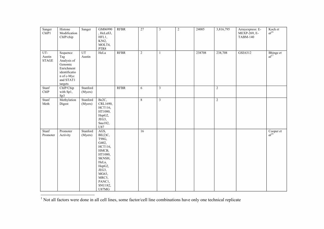
Sanger ChIP1

Histone Modification ChIP/chip

Sanger GM06990, HeLaS3, HFL1, K562, MOLT4, PTR8

RFBR 27 3 2 24005 3,816,795 Arrayexpress: E-MEXP-269, E-TABM-140

Koch et al16

UT-Austin STAGE

Sequence Tag Analysis of Genomic Enrichment identification of c-Myc and STAT1 targets

UT Austin

HeLa RFBR 2 1 238708 238,708 GSE6312 Bhinge et al17

Stanf ChIP

ChIP/Chip with Sp1, Sp3

Stanford (Myers)

RFBR 6 3 2

Stanf Meth

Methylation Digest

Stanford (Myers)

Be2C, CRL1690, HCT116, HT1080, HepG2, JEG3, Snu182, U87

8 3 2

Stanf Promoter

Promoter Activity

Stanford (Myers)

AGS, BE(2)C, T98G, G402, HCT116, HMCB, HT1080, SKNSH, HeLa, HepG2, JEG3, MG63, MRC5, PANC1, SNU182, U87MG

16 Cooper et al18

1 Not all factors were done in all cell lines, some factor/cell line combinations have only one technical replicate


UCD Ng ChIP

ChIP/Chip of E2F1, C- Myc

UC Davis

HeLa RFBR 2 3 1 384,000 2,304,000 GSE4354, GSE4306

Bieda et al19

Uppsala ChIP

ChIP/chip in HepG2

Univ Uppsala

HepG2 RFBR 9 3 1 21648 584,496 Arrayexpress E-MEXP-452

Rada-Iglesias et al20

UT-Austin ChIP

ChIP/Chip of C-Myc, E2F4

UT Austin

HeLa, 2091 fibroblast

RFBR 4 3 384,000 4,608,000 ENCODE Project Consortium21

Yale ChIP Sig

ChIP/Chip of STAT1, BAF, JUN, FOS

Yale HeLa RFBR 5 3-5

1 384,000

7,296,000 GSE2714, GSE3448, GSE3449, GSE3549, GSE3550

Euskirchen et al22

2Harvard/AFFX ChIP-chip

ChIP-chip signal

Harvard (Struhl) AFFX

HL-60, Me180

RFBR 47 3-5

2 732,046

295,746,584 GPL1789 Cawley et al23

3Yale RFBR Clusters

RFBR Enriched / Depleted regions

Yale (Gerstein)

Computational

NA NA

NA

1415 Zhang et al24

Affy RNA Signal

PolyA+ RNA Signal

Affymetrix

HL60, HeLa, GM06990

TxFrag 6 3 2 732,046 26,353,656 GPL3111 Kapranov et al25

EGASP EGASP promoter, protein coding, and pseudo gene predictions

EGASP Computational

NA NA NA 126,8394 Guigo et al26 Bajic et al27 Zheng & Gerstein28

GENCODE Genes

Gene Annotations

GENCODE

GENCODE Harrow et al29

Yale 5' RACE

Yale 5' RACE

Yale NB4 5’ RACE 1 N/A N/A 3106 3106 Trinklein et al30

2 Not all factors were done in both cell lines, not all factors were done for the same time points, not all factors were done in the same number of replicates. 3 http://dart.gersteinlab.org 4 Consists of 122,038 predicted exons, 4600 predicted promoters, 201 predicted pseudogenes


product end sequencing

GIS ChIP-PET

ChIP-PET of STAT1, p53

GI Singapore

HeLa, HCT116

Chip-PET 1 1 1 N/A 1,238,753 Wei et al31

GIS PET RNA

PETof PolyA+ RNA

GI Singapore

MCF7, HCT116

GIS-PET 1 1 1 N/A 864,964 Ng et al32

RIKEN CAGE

CAGE Predicted Gene Start Sites

RIKEN CAGE 39 1 1 5ABAAA0000001-ABAAA0345530 ABAAB0000001-ABAAB0349735 ABAAC0000001-ABAAC0081282 ABAAD0000001-ABAAD0067015 ABAAE0000001-ABAAE0143179 ABAAF0000001-ABAAF0080664 ABAAG0000001-ABAAG0038560 ABAAH0000001-ABAAH0069492 ABAAI0000001-ABAAI0048328 ABAAJ0000001-ABAAJ0074930 ABAAM0000001-ABAAM0402473 ABAAN0000001-ABAAN0138842

Carninci et al33

5 DDBJ accession numbers listed are not restricted to CAGE tags mapping to the ENCODE regions. Sequenced CAGE tags form a specific category (“MGA”) in the DDBJ database accessible at ftp://ftp.ddbj.nig.ac.jp/database/mga/


ABAAO0000001-ABAAO0248911 ABAAP0000001-ABAAP0023693 ABAAQ0000001-ABAAQ0268395 ABAAR0000001-ABAAR0014605 ABAAS0000001-ABAAS0035057 ABAAT0000001-ABAAT0035935 ABAAU0000001-ABAAU0049424 ABAAV0000001-ABAAV0037683 ABAAZ0000001-ABAAZ0022849 ABABA0000001-ABABA0100977 ABABB0000001-ABABB0055212 ABABD0000001-ABABD0010632 ABABE0000001-ABABE0179630 ABABF0000001-ABABF0125171 ABABG0000001-ABABG0024354 ABABJ0000001-ABABJ0033204 ABABL0000001-ABABL0029329 ABABM0000001-ABABM0025571 ABABN0000001-ABABN0145808 ABABO0000001-ABABO0030699 ABABP0000001-ABABP0065654 ABABQ0000001-ABABQ0321486 ABABR0000001-


ABABR0059492 ABABS0000001-ABABS0148007 ABABT0000001-ABABT0039592 ABABU0000001-ABABU0408819 ABABV0000001-ABABV0069939

Stanf RTPCR

Endogenous Transcript Levels

Stanford (Myers)

HCT116

RNA Secondary Structure prodiction

EvoFold and RNAz Predictions of RNA Secondary Structure Using TBA

UC Santa Cruz (EvoFold) and University of Vienna (RNAz)

Computational

NA NA NA Washietl et al34

Yale RNA

RNA Transcript Map

Yale Neut,Plcnta, NB4

TxFrag 5 3-10 2-3 755.000 36.995.000 GSE2671, GSE2678, GSE2679

Emanuelsson et al35 Rozowsky et al36

HapMap Coverage

Resequencing Coverage

HapMap 4

HapMap SNPs

Minor and Derived Allele Frequencies

HapMap 4 International HapMap Consortium37

NHGRI DIPs

Deletion/Insertion Polymorphisms

NHGRI (Mulliken)

Sanger Assoc

Genotype-Expression Association

Sanger GM06990 60 1 6 700 4200 Stranger et al38

SNP Recomb Hots

Recombination Hotspots from Resequencing and SNP

Oxford 270 International HapMap Consortium37


Data

SNP Recomb Rates

Recombination Rates from Resequencing and SNP Data

Oxford 270 International HapMap Consortium37


S1.1.2 Data Repository at UC Santa Cruz The ENCODE Project at UCSC web site (http://genome.ucsc.edu/ENCODE) is the main portal for sequence based data produced as part of the ENCODE Project. The site provides researchers with a number of tools that allows visualization and analysis of the data as well as the ability to download data for local analyses. Details and examples of the new ENCODE-related features are available elsewhere39, which describes the portal to the data, highlights the data that has been made available, and presents the tools that have been developed within the ENCODE project. These features are integrated with the UCSC Genome Browser40, Genome Browser Database41, and Table Browser42. As the primary data repository for sequence based data, the roles of UC Santa Cruz are (i) to collect the experimental data and analyses, (ii) to perform basic quality assurance (QA) on the submitted data, (iii) to publicly release the data with comprehensive descriptions, (iv) to provide interactive displays for integrating the ENCODE data with existing genome-wide data and (v) to provide interactive tools for analysis.

S1.1.3 Data deposition, access and analysis through Galaxy system To facilitate data exchange among different ENCODE groups during the analysis process we implemented a data repository at http://encode-upload.g2.bx.psu.edu. The repository is a web application designed to (1) provide user-friendly interface for data upload, (2) standardize naming of data files according to ENCODE guidelines, (3) automatically fragment the data into ENCODE analysis partitions, and (4) store the data so it can be accesses through the Galaxy web site (http://main.g2.bx.psu.edu).

S1.2 Experimental reproducibility and confirmation To ascertain the reliability of the data produced by the ENCODE Project, the Consortium has established two levels of data quality evaluation: data verification and data validation. “Data verification” refers to assessing the reproducibility of data recording a biochemical event assayed by a high throughput method. “Data validation” refers to confirming the biochemical function of the DNA elements identified using another, preferably independent, method on a subset of the verified data. For example, for the ChIP-chip technology, data verification involves performing at least 3 biological replicates where the top targets identified in each replica are significantly correlated. ChIP-chip validation is done by quantitative PCR (qPCR) on 48 ChIP-chip targets selected across a range of signal intensities. In the spirit of the Human Genome Project’s practice of rapid data release, the ENCODE Project requires the immediate release of verified data into the appropriate public databases, with the subsequent release of validated data. For more information on the ENCODE data release policy, see: http://www.genome.gov/12513440.

S1.3 Genome Structure Correction The type of question that we primarily address in this supplement is: Given two features of genome position, e.g. “conservation between species” and “transcription start sites” and a measure of the relatedness of these two features, e.g. base or region percentage overlap; how


significant is the observed value of the measure? How does it compare with that which might be observed “at random”? The essential difficulty in dealing with these questions is to determine the appropriate interpretation of randomness for the genome, since we observe only one of the multitudes of possible genomes that evolution might have produced for our and other species. We postulate that genomes or stretches of genomes that we observe (1) Can be thought of as a number of regions, each of which is homogenous in a sense we describe mathematically below, (2) The number of regions is small compared to the total length of the genomic segments we consider, (3) Bases that are very far from each other on the average have little to do with each other, and (4) The size of at most all but one homogenous region is small compared to the stretch that we observe. This last assumption is needed for the method we describe, but an alternative approach, which is more computationally intensive, can avoid it. There is considerable evidence for (1), (2), and (4) in the literature43-48 and (3) is clearly plausible. When we translate this into mathematical terms we obtain a formulation more general than the patently incorrect assumption that, in the homogeneous regions, bases are independent and identically distributed (the multinomial model). In fact, our formulation is more general and hence more conservative than any of the models advanced for convenience in genomics, such as Markov models and HMMs. Remarkably, it enables us to use the genomic data we have to estimate the parameters we need to perform the task(s) we outlined earlier. The formulation, for the homogenous pieces, is a well studied one in the context of time series49. The question of association for two features is now interpretable: Within the given sequence dependency structure, are the assignments of feature A and feature B to individual bases made independently? The conceptual basis of the approach is that, under our assumptions, we expect that the distribution of our statistic (over all possible genomes for this species), for a stretch of length n of the genome, can be approximated, after some renormalization by the distribution of the statistic as defined for stretches of length L where L is large, but small compared to n. This enables us to estimate the quantities we need using the empirical distribution of the values of the statistic for the n-L stretches of length L present in the data. We now sketch the actual implementation and associated statistics of the methodology. A fuller, more mathematical account is in preparation. Suppose we want to test the hypothesis that two features F and G are not associated. For example, in the expanding human transcriptome, novel sets of transcripts are regularly recorded; one can ask the question, do the base-pairs (bps) corresponding to one such set of transcripts tend to overlap with a comprehensive set of bps ostensibly conserved between multiple species more than expected at random?

To answer this question, we consider the bivariate time series (“time” here being the position in the sequence in bps), ( ) ( )( ),I t J t with n data points corresponding to the length of the


sequence. Here, ( ) 1I t = iff the bp t belongs to an instance of feature F and ( ) 1J t = iff t belongs to feature G. We assume that this time series is approximately piecewise stationary. That is, for all sets of k positions 1, , kt tK in a region , 1, ,iR i M= K , possible configurations

( ) ( )1 1, , , ,k ka b a bK of 0,1-valued pairs, and all h, 1) ( ) ( ) ( ) ( ), ,1 , ,1j j j j i j j j j iP I t h a J t h b j k R P I t a J t b j k R⎡ ⎤ ⎡ ⎤+ = + = ≤ ≤ = = = ≤ ≤⎣ ⎦ ⎣ ⎦

Note that there is no assumption on the relation between regional boundaries. Within regions this covers Markov Chains of any order, HMMs, etc. The second assumption is that, 2) M n<< where n is the total length of the region(s) under study. 3) The process ( ) ( )( ),I t J t is strongly mixing in a suitable sense – see Doukhan50. We can now represent percent bp overlap:

( ) ( )( )

I t J tS

I t= ∑

∑

and a symmetrized version of percent regional overlap, essentially as

( ) ( ) ( ) ( )( )( ) ( )( )

1 1 11 1

I t J t I t J tR

I t I t− + +

=− +

∑∑

The essential point is that, S and R and all the other statistics we discuss below are smooth functions of linear statistics, , 1, 2,...jT j = For instance,

1

2

TST

= , where

( ) ( )11

12 ( )

T n I t J t

T n I t

−

−

=

=∑∑

It is well known (see Doukhan, Chapter Theorem 3, p. 48)50, that under conditions which include the type of module we’ve considered, and the linear statistics we need, the distribution of

( )( )

T E TSD T−

is approximated by a standard normal, and that ( )E T μ= , ( )SD Tn

σ= to a first

approximation, where μ and σ don’t depend on n.


It is also standard that, by the delta method, smooth functions S of linear statistics have the same

approximations and ( )E S υ= , ( )SD Sn

τ= where υ and τ are expressible in terms of he

means, variances, and covariances of the component linear statistics (see Bickel and Doksum, Theorem 5.3.4)51. To test the hypothesis of no association, we need estimates of the expectations of these quantities, S and R under “randomness”, and then the null distributions of ˆS S− and ˆR R− . To do this we rely on the following principle, whose rationale becomes apparent in the context of time series in Politis, Romano, and Wolf52.

1. The distribution of statistics such as nS and nR based on the whole segment of length n can be approximated by a suitably renormalized version of the distribution of LS and LR , where the subscript L denotes that the statistic is computed on a sub-segment of length L, where L is << n, but large compared to the size of a homogeneous subregion51, or by

concatenating in order nL

randomly sampled subsegments as above52.

2. The distribution of LS and LR may be approximated by the empirical distribution of the statistic as defined on all n-L possible sub-segments of length L.

Relevant results are theorem 4.2.1 in Politis et al52 and theorem 3.5 and discussion in Kunsch53. Strictly speaking, the principle applies in the inhomogeneous case only if the size weighted variation between the means of the homogeneous regions is small when compared to the total variability from within the homogeneous regions after normalization of the latter by the maximum total homogeneous region size. However, if this is not the case, the analysis we pursue below is even more conservative than if the assumption holds. For regional overlap statistics we apply a Poisson approximation to the block statistics, which again does not require the above negligibility hypothesis. Fortunately, it is possible, in any case, to check whether the variability assumption is adequate by using an analytical formula for the variance of the statistics we use (Doukhan, Theorem 2, p. 47)50. This expression can be estimated correctly from the data still subject to a regularization parameter, such as L, even if the between means variability is large. Evidently, application of these methods, choosing the appropriate L in particular, is delicate. Some principles for the choice of L are discussed in Politis et al. (Ch. 12, p. 249)52, and Buhlmann and Kunsch54. We check these approaches and choices of L for internal consistency below. Testing This is not enough to give us S , R and the null distribution. We formulate the hypothesis that feature G is not enriched for feature F. No enrichment means that F and G were placed on the sequence independent of each other, but with cognizance of sequence structure. While arbitrary piecewise stationarity is assumed, note that only the two features are assumed independent.


All that is assumed for the sequence is still just piecewise stationarity. In particular, this would mean that, in a block of length L occurrences of feature F are approximately independent of feature G occurrences in a distant block of length L. This suggests that for a pair of blocks of length L, under the null, if we ascribe the feature F status of position t for 1 t L≤ ≤ in the first block to the bps in the second, which we denote ( ) ( )( )(1) (2),I t J t , then the overlap we would observe between the ‘dummy’ feature F and the true feature G would have the same distribution as the overlap we would observe between the genuine annotations in a block of length L. Hence, for a pair of blocks of length L, we have two observations of true overlap, and two observations of this ‘dummy’ overlap. In the basepair case, the true overlap is just:

( ) ( ) ( ) ( )( ) ( )

(1) (1) (2) (2)

2 (1) (2)L

I t J t I t J tS

I t I t+

=+

∑ ∑∑ ∑

the ‘dummy’ overlap is just:

( ) ( ) ( ) ( )( ) ( )

(1) (2) (2) (1)

2 (1) (2)ˆ

L

I t J t I t J tS

I t I t+

=+

∑ ∑∑ ∑

. Then, the null corresponds to the expected value of

2 2ˆ ˆ

L Ld S S= − being 0. Now, suppose we draw B pairs of blocks of length L and for each pair b compute LbLb SS 22

ˆ− , where we use the subscript to indicate that the quantity is computed based only on the two

blocks, as above.Lb

B

bS

BS

21ˆ1ˆ ∑ =

=

The empirical distribution of these B numbers is an approximation to the null distribution of

ˆL LS S− (whose mean is 0, but whose variance is too large). We now compute

Lb

B

bS

BS

21ˆ1ˆ ∑ =

= .

If B >> L, this is an adequate approximation to the value we would obtain under the hypothesis of independence of F and G. The theoretical basis for this assertion is based on the following principle. For any pair of blocks, under the null hypothesis, we know that

( ){ }1 1 2 2: 1,..., , 1,...,I t t b b L b b L= + + + + and ( ){ }1 1 2 2: 1,..., , 1,...,J t t b b L b b L= + + + + are

independent, where 1 1b + and 2 1b + are the start positions of the two blocks. Of course, our data does not have this property unless the null is true, but we can postulate that the marginal distributions of ( ){ }1 1: 1,...,I t t b b L= + + and ( ){ }2 2: 1,...,I t t b b L= + + are the same as under the null, and similarly for J. In the formulation of our statistic, we are making use of the fact that, if 1 2b b− is large, ( ) ( )( ){ }1 1, : 1,...,I t J t t b b L= + + and ( ) ( )( ){ }2 2, : 1,...,I t J t t b b L= + +

are approximately independent, whether the null is true or not. If they were exactly independent, then indeed 2

ˆLS has the correct null distribution. However, if L<<n, we expect that 1 2b b− is

large compared to L, so that the approximation is justified.


The simplest renormalization is to multiply the statistics ˆL LS S− by

2nL

, and then refer ˆnS S−

to the empirical distribution of the B renormalized LbLb SS 22ˆ− for a p-value.

A somewhat more sophisticated argument needed for regional statistics leads to estimating the covariance of the numerator ˆR R− :

( ) ( ) ( ) ( )( ) ( ) ( ) ( ) ( )( )( )(1) (1) (1) (1) (2) (1) (2) (1)1 1 1 1 1 1RN I t J t I t J t I t J t I t J t= − + + − − + +∑

( ) ( ) ( ) ( )( ) ( ) ( ) ( ) ( )( )( )(2) (2) (2) (2) (1) (2) (1) (2)1 1 1 1 1 1I t J t I t J t I t J t I t J t+ − + + − − + +∑ and the

denominator: ( ) ( ) ( ) ( )( )( ) ( ) ( ) ( ) ( )( )( )(1) (1) (1) (1) (2) (2) (2) (2)1 1 1 1 1 1RD I t J t I t J t I t J t I t J t= − + + + − + +∑ ∑

based on blocks of length L, renormalized as before, but base the computation on the identity

ˆˆ

R RRP R R t P N N tD⎡ ⎤ ⎡ ⎤− ≤ = − ≤⎣ ⎦⎣ ⎦ . The choice of L is important in these approximations.

Fortunately, in practice there is computationally negligible change in the mean or variance of the empirical distributions of ˆ

Lb LbS S− for a wide range of L. To address the regional and bp overlap

statistics, for each feature F,G pairing, we formed the ˆLb LbS S− for many L ranging from 10

times the largest feature instance to 1/5th the total sequence length, n, and selected L approximately in the center of the largest region of stability, which provided an unambiguous choice in each case. A Demonstration of the Method via Simulation In order to clearly present the importance of accounting for genomic structure in the estimation of the significance of association between two features, we have simulated two dummy features. These features occur in 100 homogeneous stretches, (with an average length of 100Kb and standard deviation 20Kb) which we concatenated to form an inhomogeneous 10Mb region. The first feature, Feature 1, is somewhat sparse, but densely clustered. Instances of this feature are around 20bps. The second, Feature 2, is ubiquitous and also densely clustered. Both features occur frequently in some homogeneous subregions, and rarely in others. On average, there are 1000 instances of Feature 1 in the 10Mb, and 10,000 instances of Feature 2. We simulated 10,000 times in order to compute the empirical distribution of feature overlap (the fraction of Feature 2 instances covered by Feature 1). This distribution was approximately Gaussian, as expected.


Supplementary Figure 1: QQplot demonstrating the approximate gaussianity of the overlap statistics from simulation

We selected one pair of features from these simulation runs to treat as our observed data, which was at the 99.9th percentile of both basepair and region overlap. We employed five methods to recapitulate the simulation distribution from this single observation. Those methods were (1) GSC, (2) independent randomization of start-sites and inter-feature-instance distances, (3) modeling features and inter-feature-instance distances with alternating exponentials (i.e. alternating Poissons), (4) randomly shuffling start positions in a self-avoiding fashion, and (5) randomly shuffling start positions in a self avoiding fashion, where feature lengths are sampled from the empirical feature-instance-length distribution. The methods returned vastly different results. From simulation, we know that the p-value associated with the region overlap statistic for this observed data is p ~ 0.005. The GSC recapitulated the simulation distribution accurately, permitting correct significance estimation in this border-line case. Each of the other methods drastically overestimated the significance of the observed data.


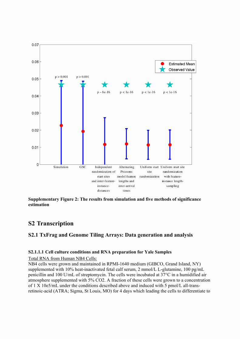
Supplementary Figure 2: The results from simulation and five methods of significance estimation

S2 Transcription

S2.1 TxFrag and Genome Tiling Arrays: Data generation and analysis

S2.1.1.1 Cell culture conditions and RNA preparation for Yale Samples Total RNA from Human NB4 Cells: NB4 cells were grown and maintained in RPMI-1640 medium (GIBCO, Grand Island, NY) supplemented with 10% heat-inactivated fetal calf serum, 2 mmol/L L-glutamine, 100 pg/mL penicillin and 100 U/mL of streptomycin. The cells were incubated at 37°C in a humidified air atmosphere supplemented with 5% CO2. A fraction of these cells were grown to a concentration of 1 X 10e5/mL under the conditions described above and induced with 5 pmol/L all-trans-retinoic-acid (ATRA; Sigma, St Louis, MO) for 4 days which leading the cells to differentiate to


neutrophils. For the monocytes differentiation, a third fraction of the NB4 cells were grown to a concentration of 1 X 10e5/mL and pre-treated with 200-nM 1,25(OH)2D3 for 8 h, then with 200-nM TPA for a total treatment time of 72 h. For each biological replicate of NB4 cells (undifferentiated), NB4 cells treated with ATRA and NB4 cells treated with TPA; total RNA was extracted using the Qiagen RNA extraction kit according to the manufacturer’s instructions. Total RNA from Human Neutrophil Cells: Human neutrophils were isolated from venous blood (freshly drawn at 8 to 9 AM) of healthy volunteers, using dextran sedimentation and centrifugation through Ficoll-Paque Plus (Pharmacia, Uppsala, Sweden), as described previously in Subrahmanyam et al55. Total RNA was extracted using the Qiagen RNA extraction kit. PolyA+ RNA from Human Placental Tissue: Triple selected polyA RNA for placenta was obtained from Ambion (Austin, TX). All RNA samples had an agilent ratio greater than 1 indicating that degradation had not occurred. All RNA samples were prepared from a pool of several different individuals.

S2.1.1.2 Cell culture conditions and RNA preparation for Affymetrix samples Cell Lines: The HL-60 acute myeloid lymphoma cell line was obtained from the American Type Culture Collection facility. Cell were maintained in Iscove's Modified Dulbecco's Medium with GlutaMAX (Invitrogen) containing 20% Fetal Bovine Serum (Invitrogen) and 1X penicillin/streptomycin (Invitrogen) in a humidified 37°C incubator with 5% CO2. For each of the three biological replicates, cultures were seeded at approximately 3x105 cells/ml and were induced with a final concentration of 1 μM ATRA (purchased from Sigma) after 2 days of growth when cultures had achieved a density of 106 cells/ml. These cultures (3 liters total for each time point) were then incubated for 2, 8, and 32 hours with ATRA or untreated (0 hour) before harvesting. Both cell viability and recovery after ATRA treatment were assessed by Trypan Blue exclusion as well as determining cell density by counting an aliquot on a hemocytometer. HeLa cell line (ATCC accession number CCL-2) was grown in DMEM media (HyClone cat# SH30022.02) supplemented with 10% fetal bovine serum (HyClone cat# SH30070.03) and 1X penicillin-streptomycin (Invitrogen cat# 10378-016). GM06990 cell line (Coriell Institute) was grown in RPMI media (HyClone cat# SH30027.02) supplemented with 15% fetal bovine serum (HyClone cat# SH30070.03) and 1X penicillin-streptomycin (Invitrogen cat# 10378-016). All cell lines were grown at 37°C at 5% CO2. CD11b Cell Surface Antigen Labeling: ATRA treated HL-60 cells were monitored for differentiation by detection of CD11b expression. Triplicate samples for each time point in each biological replicate (106 cells per sample) were centrifuged at 300xg for 10 minutes, media aspirated, and resuspended in 100 µl Label Buffer (1x Hanks Buffered Saline, 2% filtered Fetal Bovine Serum, and 0.01% sodium azide). Cells were blocked with 5 µl unlabeled isotype matched mouse IgG1κ (BD Pharmingen) on ice for 15 minutes, then washed with 2 ml ice cold Label Buffer. Cells were pelleted at 300xg for 10


minutes and resuspended in 100 µl Label buffer. Five µl of anti-CD11b antibodies or isotype controlled mouse IgG1κ coupled to Alexa 488 (BD Pharmingen) were added to each sample and incubated on ice for 30 minutes. Cells were washed twice in 2 ml Label Buffer and fixed with 2% formaldehyde in PBS. Samples were stored packed in ice and in the dark until analyzed by flow cytometry using a FACScaliber bench top cell sorter (BD Biosciences) counting 10,000 events for each triplicate sample. IgG1κ labeled samples were used to determine the amount of background fluorescence and non-specific binding. Percent of CD11b positive cells were quantitated using Cellquest Pro software. Nitroblue Tetrazolium (NBT) Reduction Assay: NBT reduction assays were performed in triplicate for each time point for each of the 3 biological replicates. Approximately 5x105 were collected by centrifugation at 300xg for 10 minutes at room temperature using a swing bucket rotor. Media was aspirated away and cells were resuspended in 100 µl of growth media. An equal volume of NBT (Roche) diluted 1:50 in PBS was then added to each sample containing 200 ng PMA (Calbiochem). Samples were incubated at 37°C for 30 minutes at which time cells were placed on microscope slides and cells were scored as either positive or negative based on the presence of dark blue formazin deposites. At least 1000 cells were counted for each of the triplicate samples and percent NBT positive cells was determined for each time point as a measure of differentiation. RNA preparation: Approximately 5x108 cells per time point per biological replicate were harvested by centrifugation and total RNA was purified using RNeasy RNA extraction kit (Qiagen) as per manufacturer’s specifications. Each sample required three columns in order to recover the majority of the RNA. PolyA RNA was then obtained from the total RNA using Oligo-tex purification kits (Qiagen) as per manufacturer’s instructions. Total RNA was isolated using Qiagen’s RNeasy protocol. Where specified, the polyA+ fraction was isolated using Qiagen’s Oligo-tex kits. Cytosolic polyA+ RNA was isolated following Qiagen’s RNeasy protocol. Total or polyA+ RNA was treated with DNAse I and then converted into double-stranded cDNA as described in Cheng et al56. 2 mg of cDNA corresponding to polyA+ RNA or 10 mg of cDNA corresponding to total RNA were hybridized to ENCODE tiling arrays as described in Cheng et al56.

S2.1.2 Description of RNA material used in the RNA mapping experiments

Supplementary Table 1: Description of RNA sources used in the RNA mapping experiments Cell line/Tissue

Number of different biological sources6

Description Stimulant (if applicable)

Time points Available

Cellular Compartment

Method of RNA profiling

Method of cDNA priming

HL60 promyeloblast, retinoic acid 0, 2, 8 Whole-cell TxFrag random

6 Refers to a number of different sources for primary cell lines or tissues assayed independently


acute promyelocytic leukemia

and 32 hrs

polyA+ RNA hexamer

HeLa cervical adenocarcinoma

Cytosolic polyA+ RNA

TxFrag random hexamer

GM06990 B-Lymphocyte, transformed with Epstein-Barr Virus

Cytosolic polyA+ RNA


NB4 Acute promyelocytic leukemia

retinoic acid 0 and 96 hrs

Whole-cell total RNA


12-O-tetradecanoylphorbol-13 acetate

0 and 72 hrs

random hexamer

Primary Neutrophils from donor blood

10 Whole-cell total RNA


Placenta Whole-cell polyA+ RNA

TxFrag, RxFrag

random hexamer - TxFrag, oligo dT - RxFrag

Brain Whole-cell polyA+ RNA

RxFrag oligo-dT

Colon Whole-cell polyA+ RNA

RxFrag oligo-dT

Heart Whole-cell polyA+ RNA

RxFrag oligo-dT

Kidney Whole-cell polyA+ RNA

RxFrag oligo-dT

Liver Whole-cell polyA+ RNA

RxFrag oligo-dT

Muscle Whole-cell polyA+ RNA

RxFrag oligo-dT

Small Intestine

Whole-cell polyA+ RNA

RxFrag oligo-dT

Spleen Whole-cell polyA+ RNA

RxFrag oligo-dT

Stomach Whole-cell polyA+ RNA

RxFrag oligo-dT

Testis Whole-cell polyA+ RNA

RxFrag oligo-dT

MCF7 mammary gland adenocarcinoma

beta-estradiol 12 hrs Whole-cell polyA+ RNA

PET oligo-dT

Whole-cell polyA+ RNA

PET oligo-dT

HCT116 colorectal carcinoma

5-fluorouracil 6hrs Whole-cell polyA+ RNA

PET oligo-dT

kidney 3 Whole-cell total RNA

CAGE random hexamer

cerebrum 4 Whole-cell total RNA

CAGE random hexamer

renal artery Whole-cell total RNA

CAGE random hexamer

ureter Whole-cell total RNA

CAGE random hexamer

urinary bladder

2 Whole-cell total RNA

CAGE random hexamer


prostate Whole-cell total RNA

CAGE random hexamer

mammary gland


CAGE random hexamer

epididymidis Whole-cell total RNA

CAGE random hexamer

adipose, processed lipoaspirate


CAGE random hexamer

dihydrotestosterone 9 days Whole-cell total RNA

CAGE random hexamer

TNF-alpha 48 hrs Whole-cell total RNA

CAGE random hexamer

preadipocyte 2 Whole-cell total RNA

CAGE random hexamer

2 dihydrotestosterone 9 days Whole-cell total RNA

CAGE random hexamer

2 TNF-alpha 48 hrs Whole-cell total RNA

CAGE random hexamer

CCD-1112Sk

fibroblast, foreskin


CAGE random hexamer

Human stem cells HS181 p52 grown on the feeder layer of CCD-1112Sk cells


CAGE random hexamer

Hep G2 hepatocellular carcinoma


CAGE Two libraries: random hexamer and oligo-dT

S2.1.3 Scoring of TARs or Yale transfrags and Affymetrix transfrags Affymetrix ENCODE microarrays have approximately 750,000 pairs of perfect-match (PM) and mismatch (MM) 25 mer oligonucleotide probes to tile all the ENCODE regions at an average spacing of 21 bp between probe starts. Technical replicas are scaled to each other using quantile normalization57 and then median scaled to 25. The probe intensities from technical replicas are combined using a sliding genomic window of 100 bps centered on the genomic coordinate of each PM probe. All probe intensities for oligonucleotides within the genomic coordinates bounded by the window are combined to estimate the pseudomedian PM-MM intensity (the pseudomedian or Lehman-Hodges estimator is computed from the median of all pairwise average of PM-MM pairs). This intensity is then assigned to the probe at the center of the window. This is repeated for each biological replicate. After this step, biological replicas were quantile normalized to each other and then for each PM probe the median of normalized intensities from biological replicas is computed. An intensity threshold is determined from negative controls; bacterial probe sequences on each microarray, which should not show hybridization signal, from the intensity that corresponds to a 5% false positive rate. Transcribed regions or transfrags (transcribed fragments) were then established by requiring a genomic region longer than 40 bps (the minimum run of the transfrag), where probe intensities above threshold are spaced less than 50 bps apart (the maximum gap allowed within the transfrag).


Distances are computed from the center nucleotide of each PM oligonucleotide probe. This scoring methodology is based on what was used in Kampa et al58 and Cheng et al56.

S2.1.4 Verification of Affymetrix genome tiling array maps

Supplementary Table 2: Validation results of Affymetrix genome tiling array maps Successful RACE reactions (%) Index

TF 5' RACE 3' RACE 5' and 3'

RACE 5' or 3' RACE

Transcription on both strands

No transcript detected

Exonic 20 19 (95) 19 (95) 16 (80) 20 (100) 19 (95) 0 (0) Intronic 90 71 (79) 77 (86) 66 (73) 79 (88) 65 (72) 11 (12) Intergenic 90 62 (69) 65 (72) 44 (49) 77 (86) 46(51) 13 (14)

Non Transfrag Regions

100 66 (66) 60 (60) 45 (45) 75 (75) 44 (44) 25 (25)

Numbers represent transfrags. Numbers in () represent % of total number of regions tested.

200 transfrags were randomly chosen from the map of HL60 cell line un-stimulated (00hr time point) with retinoic acid. The transfrags consisted of 90 intergenic transfrags, 90 intronic and 20 exonic transfrags. Intergenic or intronic transfrags were defined as correspondingly non-overlapping or overlapping the bounds of known genes from the UCSC Known Gene track on the hs.NCBIv35 version of the genome. Intergenic and intronic transfrags were selected not to overlap any mRNA or EST annotation. Information on the index transfrags, primers used for this analysis can be found at http://genome.imim.es/gencode/RACEdb. 100 non-transfrag regions that mimic transfrags in length were randomly selected throughout the non-repetitive portions of the ENCODE regions. 5’ and 3’ RACE analysis was performed on DNAseI-treated cytosolic polyA+ RNA from un-stimulated HL60 cell line for each transfrag for each strand of the genome totaling to 4 RACE reactions per transfrag. RACE reactions were performed essentially as described in Kapranov et al59 with the following modifications. cDNA synthesis for the 5’RACE was performed with a pool of 12 gene-specific primers. cDNA synthesis was done with two reverse-transcriptases: Superscript II and Thermoscript (both form Invitrogen) in two separated reactions with 50 ng of polyA+ RNA each. The cDNA reactions were pooled for the RT-PCR step. cDNA synthesis for the 3’RACE was performed with oligo-dT 3’ CDS primer as in Kapranov et al59. The cDNA was treated with RNAse A/T1 cocktail (Ambion) and RNAse H (Epicentre), purified over Qiagen’s columns and pooled for the RT-PCR step. 40 ng of purified cDNA were used as starting material for each RT-PCR reaction. Three rounds of amplifications were performed at the RT-PCR step of the RACE utilizing 3 transfrag-specific nested RT-PCR primers for both 3’ and 5’ RACE. After each round, the RT-PCR reactions were purified using QIAquick 96 PCR purification system (Qiagen) and eluted in 70 µl. 1 µl of the first round amplification was used as a template for the second round and 0.01 µl of the second round RT-PCR reaction was used as a template for the third round. Oligonucleotides 3’ CDS, UPL/UPS and NUP (Clontech SMART II RACE protocol) were used as common primes for the first, second and third round of RT-PCR. Each


round of amplification consisted of 25 cycles of PCR (94°C for 20 sec; 62°C for 30 sec; 72°C for 5 min) followed by 10 min at 72°C. Products of the final round of RT-PCRs were purified using QIAquick 96, pooled and hybridized to ENCODE arrays as described above. The maps were generated using the Tiling Analysis Software (TAS; http://www.affymetrix.com/support/developer/downloads/TilingArrayTools/index.affx) with bandwidth of 50. RACEfrags were generated using threshold of 100, maxgap =50 and minrun =50. The Affymetrix RACEfrags were filtered so that each pool contains RACEfrags that are unique to the pool. GENCODE RACEfrags were filtered against Affymetrix RACEfrags. Regions overlapping RACEfrags from the Affymetrix pools were removed. Pooling was done so that the index transfrags within each pool are at least 40 kbp apart from each other. This is to facilitate the unambiguous assignment of the parent child relationships between the index transfrag and the RACEfrag. A region (transfrag or non-transfrag) was considered to be positive for presence of a transcript of either 5’ or 3’ RACE reaction was scored positive on either strand. To control for genomic DNA contamination, 3’ RACE reactions were conducted on the 100 non-transfrag regions with the omission of the reverse transcriptase. Only 1 region was scored as positive. The data for the entire verification dataset can loaded from a centralized RACE database RACEdb located at this URL http://genome.imim.es/gencode/RACEdb. Also, the profile of each RACE reaction for each of the 300 index regions could be viewed via the links provided in this database in the UCSC browser or loaded as a BED file.

S2.1.5 Experimental reproducibility of RNA mapping using tiling arrays The experimental reproducibility of the microarray data was measured by calculating a Pearson correlation coefficient (R) between individual microarray experiments. Three tiers of correlations were calculated: (1) tier 1: correlation among different technical replicas represented by different microarrays hybridized to the same sample; (2) tier 2: correlation among different biological replicas for the same cell line or tissue and (3) tier 3: correlation among different cell lines/tissues. The correlation coefficient R was calculated based on the perfect match (PM) intensity values. The values shown in the table are R2 * 100 and represent a percent similarity. 100 would be identical, anything less than 50 quite different, above 80 very similar. As expected, the reproducibility among the technical replicas is very high ~97, followed by somewhat lower biological reproducibility at ~92. The reproducibility among different cell lines/tissues is quite low ~54, as expected for different samples. These results are quite consistent with the observation that different biological samples are quite different in the extent of un-annotated transcription and that this observation is not caused by poor reproducibility of the array data.


Supplementary Table 3: Analysis of technical versus biological reproducibility of the RNA mapping experiment obtained with the tiling arrays

Cell Line/tissue

Number of Technical (Array) Replicas

Number of Biological Replicas

Technical reproducibility (Median R2*100)

Biological reproducibility (Median R2*100)

Reproducibility among different cell lines/tissues (Median R2*100)

Summary

Total 97.0 92.2 54.3

Individual Cell line/tissue GM06990 6 3 97.2 97.6 HeLa 6 3 96.8 96.8 Placenta 7 3 96.4 93.9

HL60, 0 hours of retinoic acid treatment 6 3 92.4 93.5



HL60, 32 hours of retinoic acid treatment 6 3 98.6 92.2 NB4, Untreated 8 4 97.3 88.9

NB4, Treated with retinoic acid 8 4 97.9 91.3

NB4, treated with 12-O-tetradecanoylphorbol-13 acetate 6 3 97.6 98.4

Primary Neutrophils from donor blood 20 10 96.4 89.5


S2.2 5’-Specific Cap Analysis Gene Expression (CAGE) CAGE libraries60 were prepared using a protocol based on the described procedures in Kodzius et al61. A wide variety of human RNA libraries was used (29 distinct RNA libraries corresponding to 15 tissues) for CAGE sequencing: the content of the CAGE data repository has been described in detail elsewhere33, 62, 63 (http://fantom31p.gsc.riken.jp/cage/). CAGE technology is based on priming the first strand cDNA with an oligo-dT or a random primer, starting from total RNA and synthesize the first-strand cDNA at high temperature (55-60°C) in presence of trehalose and sorbitol to increase the full-length cDNA rate even in presence of strong secondary RNA structure. Full-length cDNA is enriched by cap-trapping, as reviewed in Harbers et al64. After chemical biotinylation, RNAseI (cleaving only single strand mRNA at any base) is used to remove any ssRNA linking the biotinylated cap and the double-strand RNA/truncated cDNA. RNA molecules hybridized with full-length cDNA molecules are left undigested, and are subsequently captured with streptavidin beads. After several stringent washings of the beads, full-length cDNAs are removed with mild alkali treatment. Following the addition of a specific linker, which contains the class-IIs restriction enzyme MmeI site next to the ligation junction with the 5’ end of cDNAs, the second strand cDNA is synthesized. Next, the cDNA is cleaved with MmeI: only the initial 20-21 nucleotides of the cDNA are left attached to the 5’-end linker, while cDNA is removed. After addition of appropriate linkers and cycles of PCR and purification, restriction-digested double strand sequencing tags are obtained. After formation of concatenamers, these are cloned and sequenced. The whole procedure is described in details elsewhere61.

S2.2.1 Mapping CAGE tags to the genome The sequenced CAGE tags were extracted and aligned to the genome by using BlastN. Only CAGE tags without base-calling problems (no “N” nucleotides in the sequence) were used for mapping, and tags mapping on multiple genomic regions (such as tags consisting of repeats) were not used for the current analysis. Only best-scoring alignments of at least 18 nucleotides length or more were chosen: if two or more alignments were best-scoring, the tag was ignored.

S2.3 Gene Identification Signature – Paired End DiTAGS (GIS-PET)

S2.3.1 Cell lines, Growth condition and RNA preparation Two human cancer cell lines were used for GIS-PET analysis. HCT116 is a human colorectal cancer cell line (ATCC#: CCL-247(tm)) and MCF7 is a human breast cancer cell line (ATCC# HTB-22(tm)). Cells grown in three ways were harvested; the log phase of MCF7 cells, MCF7 cells treated with estrogen (10nM beta-estradiol) for 12 hours and HCT116 cells treated with 5FU (5-fluorouracil) for 6 hours. Total RNA and polyA+ RNA were prepared by Trizol method and oligo-dT using standard molecular biology procedures.


S2.3.2 Full length library and PET library construction for GIS analysis Full length cDNA library was made by a modified biotinylated cap-trapper approach32, 65. Briefly, the 5’ cap structure of mRNA was first biotinylated and the 5’ intact first-strand cDNA was selected by streptavidin affinity to biotin. After second-strand synthesis, the double-strand cDNAs were cloned into a cloning vector, pGIS1, to form a full-length DNA library. This vector contains only two MmeI recognition sites in its multiple cloning sites and therefore introduces MmeI recognition sites directly flanking both ends of cDNA inserts. Purified plasmid prepared from the full-length cDNA library was digested with MmeI, end-polished with T4 DNA polymerase; and the resulting plasmids containing a pair of end tags from each terminal of the original cDNA insert were self-ligated, which were then transformed to form a transitional single-PET library. Plasmid DNA extracted from this library was digested with BamHI to release the 50bp PETs. The PETs were concatenated and cloned into the BamHI-cut pZErO-1 to form the final GIS-PET library for sequencing analysis32.

S2.3.3 PET sequencing and mapping PET sequences were extracted from vector trimmed and based called high quality sequence reads. The extraction algorithm included: 5’ vector/insert interface, a fixed size internal spacer and 3’ vector/insert interface with PET length ranged from 34 to 40 bp. The extracted PETs were then filtered to remove low-complexity sequences. Each of the PET sequences was split into 5’ tag and 3’ tag, and the tags were searched independently for matches in the compressed suffix array (CSA) of human genome assembly hg17. We mandated a minimum 16-nucleotide contiguous match for the 5’ (from nucleotide position 1 to 19) and 3’ (from 18 to the last) tags of PET to accommodate most possible variations from type II restriction enzyme slippage. The mapped tags were then paired based on the criteria that the mapping locations of 5’ and 3’ signatures of a PET sequence must be on the same chromosome, in the correct order and orientation (5’ 3’), and within appropriate genomic distance (one million base pairs)32, 66. Each PET library sequencing read generates about 10-15 PET sequences.

S2.3.4 Generation and Mapping of DiTag Sequences With respect to the ditags and polyA sequences, the RNA samples used in the ditag experiments were purified using polyT-affinity columns. The majority of the RNA species in the samples were polyA+ RNA, and since we used an oligo-dT primer (NV[T]16, N=A, T, G, C; V=T, G, C) for first-strand cDNA synthesis, the presence of a polyA stretch is guaranteed. All cDNA fragments generated for ditag analysis should thus be either derived from the polyA tail of mRNA or from internal polyA stretches. We found that 98% of ditags mapping to known transcripts matched the known 5' and 3' ends, and all the characterized 3' ends showed some kind of polyA signals in the defined region (10-30 bp upstream of 3' end), and mostly the canonical ones (like AATAAA or ATTAAA). A similar observation was reported by us previously32. There are a number of ditag-mapped 3' ends that are different from the known 3' ends. They are possible alternative 3' ends or they resulted from internal priming of the oligo-dT primer. To distinguish these two possibilities, we manually checked about 100 such "alternative" 3' ends by looking at the genomic DNA sequences +/- 50 bp from the ditag-mapped 3' ends. If it was derived from internal priming, we would see a stretch of A’s immediately after the ditag site. We


found that none (0) has such a polyA stretch, suggesting that none are due to internal priming. However, we cannot completely rule out such possibility. For this group of sequences, we did observe that a large proportion of the polyA signal is not a canonical ones (AATAAA or ATTAAA). It is known that other combinations of nucleotides can also be used as the polyA signal.

S2.4 The GENCODE Annotation Available sequence data has been used to delineate an annotation of the known genes and transcripts in the ENCODE regions by the GENCODE consortium. Details on the annotation pipeline can be found in Harrow et al29. In summary, the ENCODE regions were first subjected to a detailed manual annotation by the Havana group at the Sanger Institute; the annotators build coding transcripts based on alignments of known mRNA, EST and protein sequences to the human genome. The initial gene map delineated in this way was then experimentally refined through RT-PCR and RACE, which essentially confirmed the existence of the mRNA sequences of the hypothesized genes. Finally, the initial annotation was refined by the annotators based on these experimental results. To assess the completeness of the GENCODE annotation, and the ability of the automatic methods to reproduce it, the EGASP community experiment was organized26. EGASP was organized in two phases. In January 2005, the GENCODE annotation of 13 regions, among the 44 ENCODE regions, was publicly released: Gene and other DNA feature prediction groups world-wide were asked to submit genome annotations on the remaining 31 regions. Eighteen groups participated by submitting 30 prediction sets within four months. When the annotation of the entire set of ENCODE regions was released in May, participants, organizers and a committee of external assessors met at the Wellcome Trust Genome Campus, Hinxton, UK, for a workshop sponsored by the National Human Genome Research Institute (NHGRI) to compare the GENCODE annotation, with the predictions by the groups. While the computational methods were accurate to predict the individual exons, they were less accurate when linking exons together into gene structures, with the best of the programs being able to resolve about 40% of the complete gene structures inferred by the human annotators. On the other hand more than 12,000 unique exons were predicted by the programs, which were not included in the GENCODE annotation. Experimental verification of a subset of them by RT-PCR yielded only about 3% verification rate (see Guigó et al26 for details).

S2.4.1 The GENCODE Consortium The GENCODE consortium (http://genome.imim.es/GENCODE) was formed to identify and map all protein-coding genes within the ENCODE regions. This is achieved by a combination of initial manual annotation by the HAVANA team (http://www.sanger.ac.uk/HGP/havana/), experimental validation by the GENCODE consortium, and a refinement of the annotation based on these experimental results. The HAVANA group divides gene features into eight different categories of which only the first two (known and novel CDS) are confidently predicted to be protein-coding genes. The common factor between all annotated gene structures is that they must be supported by transcriptional evidence, through homology to cDNA, EST and/or protein sequences. Eight different loci categories were used to fully classify the annotation produced for the ENCODE project29.


Extensive experimental validation was used to confirm the initial manual annotation. First, 5’ raid amplification of cDNA ends (RACE) was performed on 420 coding loci in 12 different tissues and resulted in 229 loci being confirmed by sequenced RACE products. In addition RT-PCR was used to verify all 360 splice junctions representing 161 novel and putative transcripts, resulting in 37% of novel transcripts being confirmed and 19% or the putative transcripts. RT-PCR verification of 1215 splice junctions identified by computational gene prediction algorithms, but not manually annotated by GENCODE, revealed only 2 (0.2%) splice junctions could be confirmed, suggesting that few intergenic coding loci remained unannotated29.

S2.4.2 GENCODE Loci classification as defined in Harrow, et al29 -known genes are identical to human cDNA or protein sequences and identified by a GeneID in Entrez Gene ( http://www.ncbi.nlm.nih.gov/entrez/query .fcg?db=gene). -novel CDSs (CoDing Sequence) have an open reading frame (ORF) and are identical, or have homology, to cDNAs or proteins but do not fall in the above category; these mRNA sequences are submitted to public databases, but they are not yet represented in Entrez Gene or have not yet received an official gene name from the nomenclature committee ((http://www.gene.ucl.ac.uk/nomenclature/). They can also be novel in the sense that they are not yet represented by an mRNA sequence in the species concerned. -novel transcripts are as above but no ORF can be unambiguously assigned; these can be genuine non-coding genes or they may be partial protein-coding genes supported by limited evidence. They should be supported by at least three ESTs from independent sources (not originating from the same clone identifier). -putative genes are identical, or have homology, to spliced ESTs but lack a significant ORF and polyA features; these are generally short two or three exon genes or gene fragments. -pseudogenes (assumes no expressed evidence) have homology to proteins but generally suffer from a disrupted CDS and an active homologous gene can be found at another locus. This category can be further subdivided into processed or unprocessed pseudogenes. Sometimes these entries have an intact CDS or an open but truncated ORF, in which case there is other evidence used (for example genomic polyA stretches at the 3’ end) to classify them as a pseudogene. -transcribed pseudogenes are not currently given a separate tag within GENCODE and are handled by creating a pseudogene object and an overlapping transcript object with the same locus name. -TEC (To be Experimentally Confirmed). This is used for non-spliced EST clusters that have polyA features. This category has been specifically created for the ENCODE project to highlight regions that could indicate the presence of novel protein coding genes that require experimental validation, either by 5’ RACE or/RT-PCR to extend the transcripts or by confirming expression of the putatively-encoded peptide with specific antibodies. -artefact gene is used to tag mistakes in the public databases (Ensembl/SwissProt/ Trembl). Usually these arise from high-throughput cDNA sequencing projects, which submit automatic annotation sometimes resulting in erroneous CDSs that are, for example, 3’ UTRs.

S2.4.3 Expression levels of GENODE transcripts We investigated the expression levels of GENCODE transcripts using the signal levels from the 11 experiments used to detect TxFrags.(http://genome.ucsc.edu/cgi-


bin/hgTables?org=Human&db=hg17&hgsid=86335460&hgta_doMainPage=1&hgta_group=encodeTxLevels ; tracks Yale Tar, Yale RNA, Affy RNA Signal, Affy Transfrags) Each experiment was analysed separately because the threshold level used for calling TxFrags could vary substantially from experiment to experiment. Each probe was classified according to its coverage by both the TxFrags detected in the particular experiment under consideration and the GENCODE annotated exons. The exon type classes were single-cover ie annotated as being involved in only a single transcript, multi-cover ie covered by annotation from multiple transcripts, coding ie covered by annotation from a transcript with a CDS region and non-coding (NC) ie covered by a transcript with no identified CDS. Probes partially overlapping a particular exon type were assigned that type hence any given probe could fall into none, any or all four of the exon classes. This allowed us to omit boundary-overlapping probes and probes belonging to more than one class from the analyses. We looked at the distribution of signal levels for the probes which fell both in transfrags and in only one of the following annotation classes 'single-cover NC', 'single-cover coding', 'multi-cover NC' and 'multi-cover coding' in order to compare the expression levels of the different exon classes. The distributions of signal level were broadly similar for the four annotation classes in all the tissues and cell lines examined. For an example see Supplementary Figure 3.


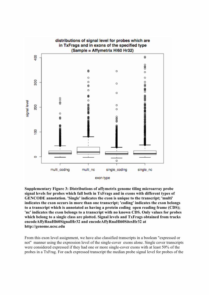
Supplementary Figure 3: Distributions of affymetrix genome tiling microarray probe signal levels for probes which fall both in TxFrags and in exons with different types of GENCODE annotation. 'Single' indicates the exon is unique to the transcript; 'multi' indicates the exon occurs in more than one transcript; 'coding' indicates the exon belongs to a transcript which is annotated as having a protein coding open reading frame (CDS); 'nc' indicates the exon belongs to a transcript with no known CDS. Only values for probes which belong to a single class are plotted. Signal levels and TxFrags obtained from tracks encodeAffyRnaHl60SignalHr32 and encodeAffyRnaHl60SitesHr32 at http://genome.ucsc.edu From this exon level assignment, we have also classified transcripts in a boolean "expressed or not" manner using the expression level of the single-cover exons alone. Single cover transcripts were considered expressed if they had one or more single-cover exons with at least 50% of the probes in a TxFrag. For each expressed transcript the median probe signal level for probes of the


specified type was extracted. The distributions of these median values for coding single-cover and NC single-cover transcripts were similar to one another in all the tissues and cell lines indicating similar levels of expression for the coding and NC transcripts (see Supplementary Figure 4).

Supplementary Figure 4: Distributions of transcript median probe signal level of single-cover probes from transcripts having at least one exon annotated as unique to the transcript expressed. Exons were considered expressed if at least half the probes they contained were also contained in TxFrags. 'Coding' indicates the transcript is annotated as having a protein coding open reading frame (CDS); 'nc' indicates the transcript has no known CDS. Signal levels and TxFrags obtained from tracks encodeAffyRnaHl60SignalHr32 and encodeAffyRnaHl60SitesHr32 at http://genome.ucsc.edu


S2.5 Generation of Transcript Maps

S2.5.1 Generation of merged maps 28 maps were generated that describe the union of the following sources of annotations: 1. CAGE tags from Riken 2. PETs from Singapore 3. GENCODE exons (only exons of known and validated genes are considered here). 4. Filtered (see below for filtering process) TARS from Yale 5. Filtered (see below for filtering process) from Affymetrix. The set of CAGE tags, PETs and GENCODE exons is same for each file. Only the TAR or transfrag content varied. There are 22 maps for each cell line/time point (11 for each strandless and stranded content). In addition, there are 2 maps for union of all Affymetrix and Yale array data, 2 files for polyA+ RNA data and 2 files for Total RNA data (see Table 2 for the list of cell lines and RNA sources). The strandless files were generated by ignoring strand information whereas the stranded files were generated on a strand-by-strand basis.

S2.5.2 Generation of 5' and 3' transcript end maps Briefly, a comprehensive map of all nucleotides within the ENCODE regions that have evidence of being 5' or 3' ends of genes was generated. The source data for the generation was the GENCODE annotation of transcript boundaries (gives connected 5' and 3' edges), the PET dataset (gives connected 5' and 3' edges), and the CAGE dataset (gives only 5' edges). For the maps, only the start or end nucleotide position of a transcript was considered. The confidence of ends identified by PET and CAGE data is increased with the number of tags mapping to the same position. Any nucleotide within the ENCODE regions that had a 5' or a 3'end indicated by any of the above data sources was included in the map, and the level of support for each data source was annotated. In detail, the GENCODE transcripts were divided into their respective Havana categories, and the support level counted for each of these sets for 5' and 3' positions. The Ditag count is the total number of PETs starting (in the 5' case) or ending (3'case) at the position (including identical tags), regardless of cell line. The CAGE tag count is the total number of CAGE tags starting in the position (5' case), regardless of cell line or tissue source. For parsing issues, the cage count is reported in the 3' cases also, where it always is zero. In those cases where 3' ends and 5' ends can be connected by GENCODE or Ditag data, this is indicated. The map should be considered a baseline of all evidence of 5' and 3' ends within the ENCODE regions, and sites corresponding to a given level of confidence can easily be extracted from the map. An important consideration is that the ends are at nucleotide level scale: there are many cases of multiple ends that are closely located (often the next nucleotide positions). This should be considered if the goal of extraction is to define promoter regions – in that case, clustering nearby locations into one unit is more relevant approach.


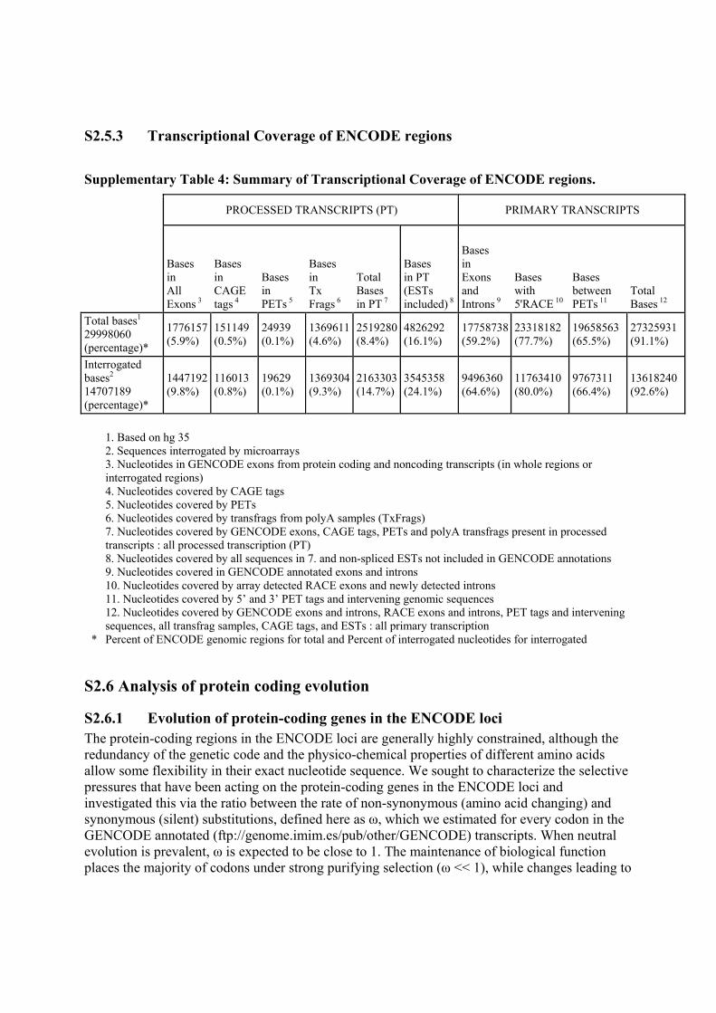
S2.5.3 Transcriptional Coverage of ENCODE regions

Supplementary Table 4: Summary of Transcriptional Coverage of ENCODE regions.

PROCESSED TRANSCRIPTS (PT) PRIMARY TRANSCRIPTS

Bases in All Exons 3

Bases in CAGE tags 4

Bases in PETs 5

Bases in Tx Frags 6

Total Bases in PT 7

Bases in PT (ESTs included) 8

Bases in Exons and Introns 9

Bases with 5'RACE 10

Bases between PETs 11

Total Bases 12

Total bases1 29998060 (percentage)*

1776157 (5.9%)

151149 (0.5%)

24939 (0.1%)

1369611(4.6%)

2519280(8.4%)

4826292 (16.1%)

17758738 (59.2%)

23318182 (77.7%)

19658563 (65.5%)

27325931 (91.1%)

Interrogated bases2 14707189 (percentage)*

1447192 (9.8%)

116013 (0.8%)

19629 (0.1%)

1369304(9.3%)

2163303(14.7%)

3545358 (24.1%)

9496360 (64.6%)

11763410 (80.0%)

9767311 (66.4%)

13618240 (92.6%)

1. Based on hg 35 2. Sequences interrogated by microarrays 3. Nucleotides in GENCODE exons from protein coding and noncoding transcripts (in whole regions or interrogated regions) 4. Nucleotides covered by CAGE tags 5. Nucleotides covered by PETs 6. Nucleotides covered by transfrags from polyA samples (TxFrags) 7. Nucleotides covered by GENCODE exons, CAGE tags, PETs and polyA transfrags present in processed transcripts : all processed transcription (PT) 8. Nucleotides covered by all sequences in 7. and non-spliced ESTs not included in GENCODE annotations 9. Nucleotides covered in GENCODE annotated exons and introns 10. Nucleotides covered by array detected RACE exons and newly detected introns 11. Nucleotides covered by 5’ and 3’ PET tags and intervening genomic sequences 12. Nucleotides covered by GENCODE exons and introns, RACE exons and introns, PET tags and intervening sequences, all transfrag samples, CAGE tags, and ESTs : all primary transcription

* Percent of ENCODE genomic regions for total and Percent of interrogated nucleotides for interrogated

S2.6 Analysis of protein coding evolution

S2.6.1 Evolution of protein-coding genes in the ENCODE loci The protein-coding regions in the ENCODE loci are generally highly constrained, although the redundancy of the genetic code and the physico-chemical properties of different amino acids allow some flexibility in their exact nucleotide sequence. We sought to characterize the selective pressures that have been acting on the protein-coding genes in the ENCODE loci and investigated this via the ratio between the rate of non-synonymous (amino acid changing) and synonymous (silent) substitutions, defined here as ω, which we estimated for every codon in the GENCODE annotated (ftp://genome.imim.es/pub/other/GENCODE) transcripts. When neutral evolution is prevalent, ω is expected to be close to 1. The maintenance of biological function places the majority of codons under strong purifying selection (ω << 1), while changes leading to


molecular adaptation between species may reveal themselves through excessive numbers of non-synonymous substitutions (ω > 1). In the context of ENCODE, estimates of ω provide another useful function, which is to distinguish likely correct annotations of open reading frames from false ones. Studies of selection are dependent on highly accurate alignments, as local alignment mistakes may cause an apparent excess of non-synonymous changes to be observed. The aligners used to align the ENCODE genomic sequences operate at the DNA level, and do not explicitly look for protein-coding sequence. To produce improved protein alignments, we assumed that the genome aligners correctly identified regions orthologous to the human exons and these were extracted, along with flanking sequences, and re-aligned using a protein-aware version of the prank aligner67. The resulting exon alignments were used to compute sitewise and exon-wide estimates of ω using SLR (see Section S2.6.3 ) Our results show that, in line with expectations, 45% and 72% of codons are under strong (ω < 0.05) or moderately strong (ω < 0.25) purifying selection, respectively. Additionally, 81% of exons are highly constrained, with an exon-wide mean ω estimate smaller than 0.05 (Supplementary Figure 5, histogram). Of these exons, 5.5% have at least one site estimated to have ω significantly greater than 1. A single site (at nucleotide position 1740) in a highly conserved exon of ACSL6, for example, was inferred to have undergone adaptive evolution (Supplementary Figure 5, upper panel). In our analyses we noticed a small but significant fraction of exons where the expected pattern of substitution is not observed. A small fraction (3.3%) of exons have a mean ω estimate greater than 0.25, caused by aberrant estimates at multiple sites. A proposed exon within GRM8, for example (Supplementary Figure 5, lower panel), does not appear to evolve with the usual evolutionary dynamics associated with protein-coding sequences; only one of the three proposed alternative transcripts (variant 003) for this gene contains the unusual exon, and this transcript continues in a different reading frame from the others then terminates early. To further investigate our results, we devised a novel method to score each exon according to its overall tendency to conform to a ‘background’ distribution of sitewise ω values (see Section S2.6.3 ) Proposed exons or transcripts were ranked by this ‘oddness score’, allowing the easy identification of unusual exons. Aberrant patterns of selection may be explained by interesting biological phenomena, such as functionality in only a subset of species or exons having coding and non-coding functions, but are also consistent with errors in annotation and/or the identification of orthologous sequences. An arbitrary threshold for the ‘oddness’ score can be used to filter out the most implausible-looking exons/transcripts from further analyses. The results of our analyses are available via http://www.ebi.ac.uk/goldman-srv/encode, including prank alignments, sitewise estimates of ω, and lists of GENCODE annotated exons and transcripts ordered according to their ‘oddness’ score. Summarized versions of our protein analyses are also provided as custom tracks within the UCSC Genome Browser.


Supplementary Figure 5: Examples of sitewise ω analyses. The upper panel is from the ACSL6 gene of ENCODE target region ENm002. At the top, the colored horizontal lines and legend indicate the exons that contribute to each proposed transcript variant (001, ... , 012). The color of sitewise ω estimates (circles) and their confidence intervals (bars) denote the inferred mode of selection acting: blue: purifying selection; grey: unclassified; red: adaptive evolution (also highlighted with a pink background). Below this is a per-nucleotide measure of conservation, with abnormally fast sites colored orange (3rd codon positions) or red (1st or 2nd codon positions). The black bars at the bottom record the number of sequences available at each alignment position. The upper panel is typical of a good protein sequence alignment. The exon boxed in red has a typical exon-wide mean ω, indicated by the arrow showing its position relative to the distribution of the means from the full data. Note the single site (position 1740) for which significant positive selection is inferred. The lower panel is from GRM8 (Enm014). The exon boxed in purple (only present in transcript variant 003) has an atypical mean ω value, and comprises many sites inferred to have neutral or positively selected evolutionary dynamics. The preceding exon is not unusual; in the following one, variant 003 is in a different reading frame, terminates early and again has an unusual pattern of sitewise ω estimates. This is suggestive that variant 003 is under unusual selective pressures or is not protein coding.

S2.6.2 Consequences of the analysis The availability of homologous sequence from many vertebrate species enables the evolutionary history of human proteins to be analyzed at the molecular level, giving insights into function and


adaptation. The depth of sequence provided by the ENCODE project enabled us to analyze all exons from proposed transcripts for selective pressures, providing useful estimates down to single codon resolution. Our results show that the majority (81%) of protein-coding exons in the ENCODE regions have evolved under strong purifying selection. A small fraction of these highly conserved exons (5.5%) have evidence of adaptive evolution at one or more of their codon sites, suggesting that continual adaptation is rare. A significant fraction of proposed protein-coding exons appear to evolve in an atypical manner, with aberrant patterns of selective pressures acting upon them. There is unlikely to be a single specific cause of such unusual patterns of selection. It may be attributable to interesting biological phenomena that induce unusual forms of selection, including the scenario that the annotated region is not functional in some target species. The aberrant patterns may also result from coding sequence overlapping other evolutionarily constrained features, leading to purifying selection acting on both synonymous and non-synonymous changes in a manner not captured by this analysis. Alternatively, the unusual patterns may result from methodological problems, including errors in transcript annotation, poor sequence coverage, and alignment mistakes. Differentiating between these possibilities is difficult and we have concentrated our methods to highlight unusual patterns for further study. Currently, we advocate caution with accepting all proposed transcript variants as protein-coding: a region that is transcribed and spliced, even when it contains an open reading frame, may not necessarily code for a protein.

S2.6.3 Method for determining the rates of evolution in protein-coding genes To improve the quality of the protein alignments, protein-coding exons with 200 bases of upstream and downstream flanking regions were extracted from the TBA alignments, and the sequences were re-aligned using the prank aligner67. This aligner exploits gene structure, with its varying patterns of evolutionary dynamics, and ensures that the alignments satisfy certain biological requirements such as ensuring the sequences begin and end with a UTR, and that the protein-coding regions are flanked by start/stop codons or donor/acceptor splice sites. The new alignments were trimmed by removing the upstream and downstream UTR regions, the two nucleotides at the beginning and end of each exon that may be under strong selection for the splicing function, and possibly one or two nucleotides to correct the exon into the first reading frame. Columns having alignment gaps in the human sequence were removed, as were the incomplete codons, caused by (e.g.) non-reading frame alignment gaps, and stop codons. Only exons from complete transcripts were included in later analyses. Taking the alignments and phylogenetic trees, estimates and confidence intervals for the non-synonymous to synonymous rate ratio, ω, were obtained for each aligned site using the SLR method68. The method requires quantities, such as the length of branches and codon composition, that are considered common to all sites and these were estimated on a per-gene basis by concatenating all constituent exons. Confidence intervals were calculated for each estimate to ensure that the results are useful. We devised a novel method to score each exon according to its constituent sites’ overall tendency to conform to the ‘background’ distribution of sitewise ω values. We assume this background is largely representative of true protein-coding genes, and quantify the deviation of each exon’s ω estimates from this background with Kolmogorov-Smirnov-like test statistics accounting for the uncertainty in these estimates. This provides an ‘evolutionary oddness’ score for each exon; gene transcripts can be scored according to the maximum oddness score attained by any of their exons.


S2.7 Expression and confirmation of GENCODE transcripts and unusual splice variants

S2.7.1 Confirmation of unusual splice variants Reconfirmation of 144 unusual splice variant transcripts was experimentally attempted by RT-PCR and sequencing of a specific splice-junction in a panel of 24 human tissues. The selected splice junction could either be the result of exon-skipping (91 cases) or presence of an exon specific to the non-canonical transcript variant (53 cases). A positive amplification was found for 36 out of 144 cases (see section S2.7.3 ) This approach has been shown to confirm 87% (84/96) and 12% (6/50) of exon-exon junctions of known human genes and novel human genes identified using the chicken genome as reference29, 69. Thus the rate of confirmation observed here (25%), suggests that these transcripts might be less abundant than the canonical ones. However, exon-exon junction that yielded positive results were found expressed in an average of 8.9 tissues out of the 24 tested suggesting that the non-canonical splice variants do not present extremely restricted expression patterns.

S2.7.2 Materials and Methods 24 human cDNAs (brain, heart, kidney, spleen, liver, colon, small intestine, muscle, lung, stomach, testis, placenta, skin, PBLs, bone marrow, fetal brain, fetal liver, fetal kidney, fetal heart, fetal lung, thymus, pancreas, mammary glands, prostate) were independently mixed with JumpStart REDTaq ReadyMix (Sigma) and 4 ng/ul primers (Sigma-Genosys) using a BioMek 2000 robot (Beckman) as described and modified70. RT-PCR oligonucleotides were designed with primer 3 (http://frodo.wi.mit.edu/cgi-bin/primer3/primer3_www.cgi) with default parameters. The first 10 cycles of PCR amplification were performed with a touchdown annealing temperature decreasing from 60 to 50ºC; annealing temperature of the next 30 cycles was carried out at 50ºC. Amplimers were separated on Ready-to-Run precast gels (Pharmacia). When the tested exon-exon splice junction was the result of an exon specific to the non-canonical transcript the amplimers were sequenced directly. On the contrary tested exon-exon junction that result from exon-skipping were purified from gel. This procedure allowed separating and sequencing the two amplimers corresponding to both the canonical and the non-canonical transcripts

S2.7.3 Table in the supplemental Excel spreadsheet This table is included in the attached Excel spreadsheet on the worksheet labeled Section S2.7.3.


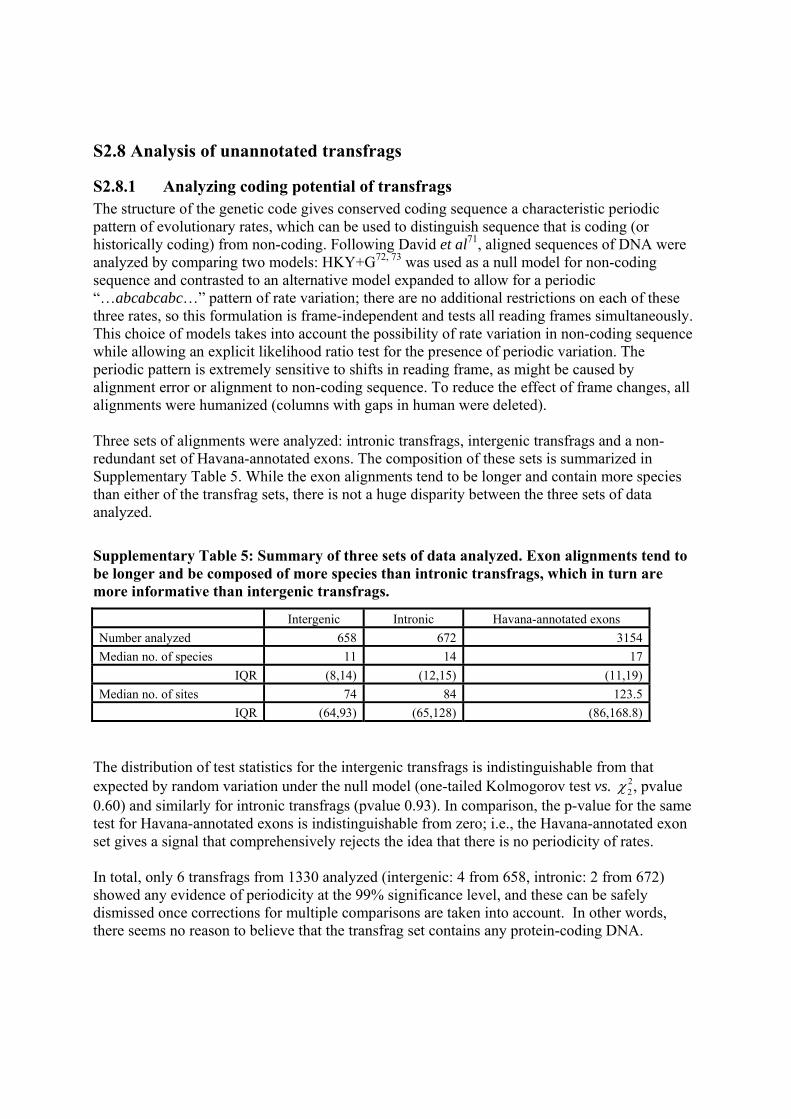
S2.8 Analysis of unannotated transfrags

S2.8.1 Analyzing coding potential of transfrags The structure of the genetic code gives conserved coding sequence a characteristic periodic pattern of evolutionary rates, which can be used to distinguish sequence that is coding (or historically coding) from non-coding. Following David et al71, aligned sequences of DNA were analyzed by comparing two models: HKY+G72, 73 was used as a null model for non-coding sequence and contrasted to an alternative model expanded to allow for a periodic “…abcabcabc…” pattern of rate variation; there are no additional restrictions on each of these three rates, so this formulation is frame-independent and tests all reading frames simultaneously. This choice of models takes into account the possibility of rate variation in non-coding sequence while allowing an explicit likelihood ratio test for the presence of periodic variation. The periodic pattern is extremely sensitive to shifts in reading frame, as might be caused by alignment error or alignment to non-coding sequence. To reduce the effect of frame changes, all alignments were humanized (columns with gaps in human were deleted). Three sets of alignments were analyzed: intronic transfrags, intergenic transfrags and a non-redundant set of Havana-annotated exons. The composition of these sets is summarized in Supplementary Table 5. While the exon alignments tend to be longer and contain more species than either of the transfrag sets, there is not a huge disparity between the three sets of data analyzed.

Supplementary Table 5: Summary of three sets of data analyzed. Exon alignments tend to be longer and be composed of more species than intronic transfrags, which in turn are more informative than intergenic transfrags.

Intergenic Intronic Havana-annotated exons Number analyzed 658 672 3154 Median no. of species 11 14 17

IQR (8,14) (12,15) (11,19) Median no. of sites 74 84 123.5

IQR (64,93) (65,128) (86,168.8) The distribution of test statistics for the intergenic transfrags is indistinguishable from that expected by random variation under the null model (one-tailed Kolmogorov test vs. χ2

2, pvalue 0.60) and similarly for intronic transfrags (pvalue 0.93). In comparison, the p-value for the same test for Havana-annotated exons is indistinguishable from zero; i.e., the Havana-annotated exon set gives a signal that comprehensively rejects the idea that there is no periodicity of rates. In total, only 6 transfrags from 1330 analyzed (intergenic: 4 from 658, intronic: 2 from 672) showed any evidence of periodicity at the 99% significance level, and these can be safely dismissed once corrections for multiple comparisons are taken into account. In other words, there seems no reason to believe that the transfrag set contains any protein-coding DNA.


The corresponding numbers for the Havana exons are 2661 significant from 3154, with 2252 remaining significant after correcting for multiple comparisons using the procedure of Hochberg74. This is clearly a very different signal from the transfrags. The exons not significant represent some mixture of Havana-annotated exons that are not actually protein-coding; or that have poor Encode alignments; or where the statistical power of the test is not enough to find the coding signal (of course, there are also reasons why some of the transfrags could be coding but not indicated as such by these tests). Supplementary Figure 6 shows that the estimated rates for the transfrags tend to be equal (a = b = c), consistent with being non-coding, whereas the Havana-annotated exons tend to be dominated by a single rate as might be occur if every third position is less constrained than its neighbours. Supplementary Figure 7 shows the performance of the periodicity test, if used to distinguish between annotated exon “coding sequence” and transfrags “non-coding”.

Supplementary Figure 6: Estimated rates for transfrags and Havana-annotated exons. Upper left: The three rates are constrained so each is positive and their sum is 3.0, and so lie in a simplex (an equilateral triangle). The ambiguity over reading frame is resolved by


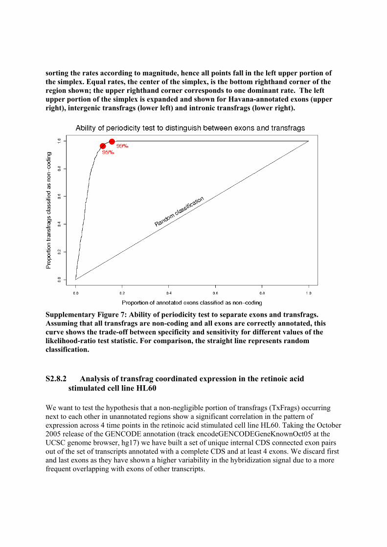
sorting the rates according to magnitude, hence all points fall in the left upper portion of the simplex. Equal rates, the center of the simplex, is the bottom righthand corner of the region shown; the upper righthand corner corresponds to one dominant rate. The left upper portion of the simplex is expanded and shown for Havana-annotated exons (upper right), intergenic transfrags (lower left) and intronic transfrags (lower right).

Supplementary Figure 7: Ability of periodicity test to separate exons and transfrags. Assuming that all transfrags are non-coding and all exons are correctly annotated, this curve shows the trade-off between specificity and sensitivity for different values of the likelihood-ratio test statistic. For comparison, the straight line represents random classification.

S2.8.2 Analysis of transfrag coordinated expression in the retinoic acid stimulated cell line HL60

We want to test the hypothesis that a non-negligible portion of transfrags (TxFrags) occurring next to each other in unannotated regions show a significant correlation in the pattern of expression across 4 time points in the retinoic acid stimulated cell line HL60. Taking the October 2005 release of the GENCODE annotation (track encodeGENCODEGeneKnownOct05 at the UCSC genome browser, hg17) we have built a set of unique internal CDS connected exon pairs out of the set of transcripts annotated with a complete CDS and at least 4 exons. We discard first and last exons as they have shown a higher variability in the hybridization signal due to a more frequent overlapping with exons of other transcripts.


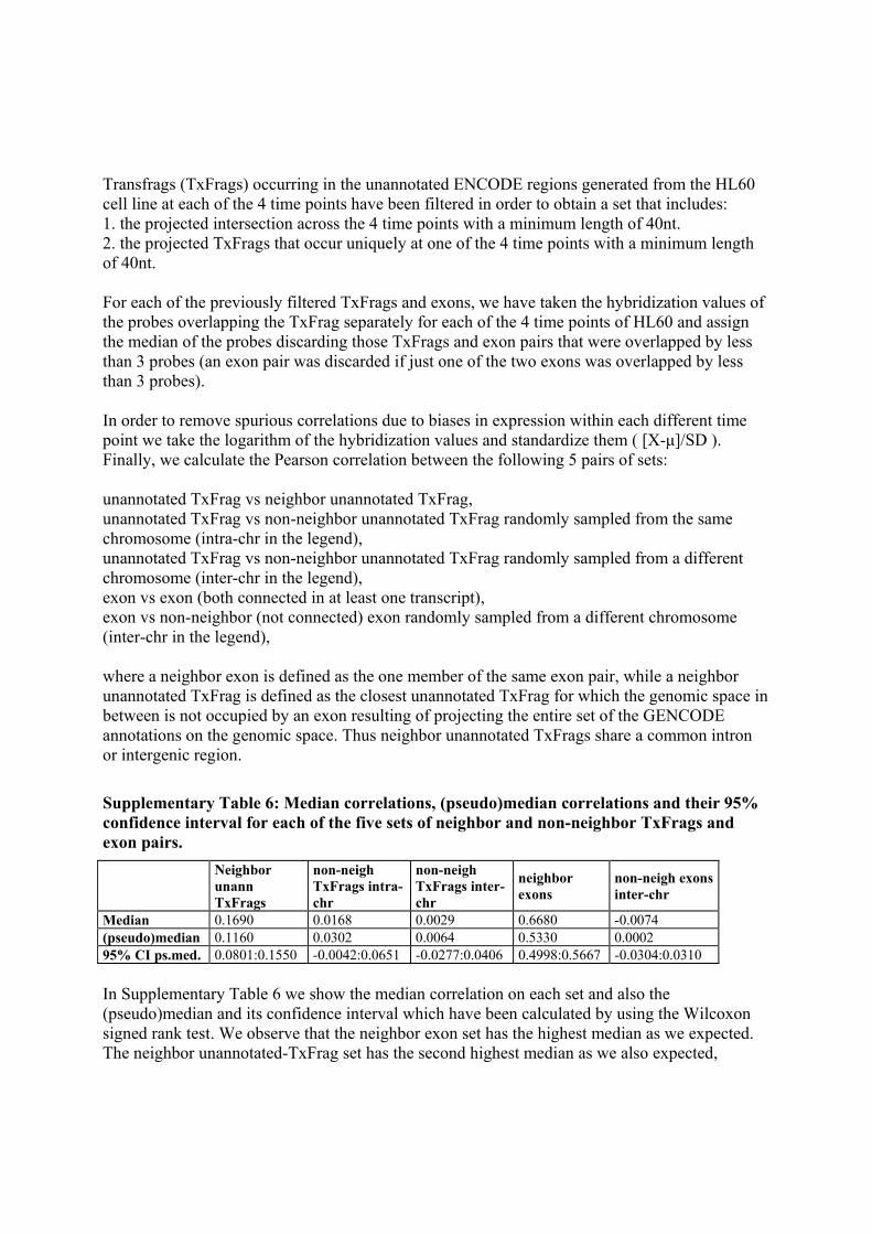
Transfrags (TxFrags) occurring in the unannotated ENCODE regions generated from the HL60 cell line at each of the 4 time points have been filtered in order to obtain a set that includes: 1. the projected intersection across the 4 time points with a minimum length of 40nt. 2. the projected TxFrags that occur uniquely at one of the 4 time points with a minimum length of 40nt. For each of the previously filtered TxFrags and exons, we have taken the hybridization values of the probes overlapping the TxFrag separately for each of the 4 time points of HL60 and assign the median of the probes discarding those TxFrags and exon pairs that were overlapped by less than 3 probes (an exon pair was discarded if just one of the two exons was overlapped by less than 3 probes). In order to remove spurious correlations due to biases in expression within each different time point we take the logarithm of the hybridization values and standardize them ( [X-μ]/SD ). Finally, we calculate the Pearson correlation between the following 5 pairs of sets: unannotated TxFrag vs neighbor unannotated TxFrag, unannotated TxFrag vs non-neighbor unannotated TxFrag randomly sampled from the same chromosome (intra-chr in the legend), unannotated TxFrag vs non-neighbor unannotated TxFrag randomly sampled from a different chromosome (inter-chr in the legend), exon vs exon (both connected in at least one transcript), exon vs non-neighbor (not connected) exon randomly sampled from a different chromosome (inter-chr in the legend), where a neighbor exon is defined as the one member of the same exon pair, while a neighbor unannotated TxFrag is defined as the closest unannotated TxFrag for which the genomic space in between is not occupied by an exon resulting of projecting the entire set of the GENCODE annotations on the genomic space. Thus neighbor unannotated TxFrags share a common intron or intergenic region.

Supplementary Table 6: Median correlations, (pseudo)median correlations and their 95% confidence interval for each of the five sets of neighbor and non-neighbor TxFrags and exon pairs.

Neighbor unann TxFrags

non-neigh TxFrags intra-chr

non-neigh TxFrags inter-chr

neighbor exons

non-neigh exons inter-chr

Median 0.1690 0.0168 0.0029 0.6680 -0.0074 (pseudo)median 0.1160 0.0302 0.0064 0.5330 0.0002 95% CI ps.med. 0.0801:0.1550 -0.0042:0.0651 -0.0277:0.0406 0.4998:0.5667 -0.0304:0.0310 In Supplementary Table 6 we show the median correlation on each set and also the (pseudo)median and its confidence interval which have been calculated by using the Wilcoxon signed rank test. We observe that the neighbor exon set has the highest median as we expected. The neighbor unannotated-TxFrag set has the second highest median as we also expected,


although the strength of the median correlation is not very high (0.17) but it is about 10 times larger than the non-neighbor TxFrag intra-chromosomal set, about 58 times larger than the non-neighbor TxFrag inter-chromosomal set and about 23 times larger than the non-neighbor exon set. The confidence interval (CI) for the neighbor sets of exons and unannotated TxFrags does not include the value of 0 correlation meaning that the correlation, although small in the case of the unannotated TxFrags, can be considered significant, while the CIs for the other three non-neighbor sets do not overlap the CI of the neighbor sets and they do include the value 0 implying that the median correlation in these three sets cannot be considered significant.

Supplementary Figure 8: Distribution of the median correlation throughout the five sets of neighbor and non-neighbor TxFrags and exon pairs

In Supplementary Figure 8 we show the distribution of the median correlation across the five sets (vertical bars) together with the accumulated minimum number of pairs at a particular median correlation (solid lines). For instance, about 40% of the neighbor exon pairs have at least a median correlation of 0.8 while this occurs to about 20% of the neighbor TxFrag pairs occurring in unannotated regions.


S2.9 RACE and Genome Tiling Arrays: Data generation and analysis

S2.9.1 Data generation for RACE/array of known protein-coding genes 5’-RACEs were performed on polyA+ RNAs from 12 human tissues (brain, heart, kidney, spleen, liver, colon, small intestine, muscle, lung, stomach, testis, placenta, all BD Clontech) using the BD SMARTTM RACE cDNA amplification kit (BD Clontech Cat. No.634914). Double-stranded cDNA synthesis, adaptor ligations to the synthesized cDNA and 25 µl final volume RACE reactions were performed according to the manufacturers’ instructions. RACE primers were designed with primer 3 (http://frodo.wi.mit.edu/cgi-bin/primer3/primer3_www.cgi) with the following parameters: 23 ≤ primer size ≤ 27, optimal size=25, 68°C ≤ primer Tm ≤ 72°C, optimal Tm = 70°C, 50% ≤ primer GC percentage ≤ 70%. 15 µl aliquots of 80 to 100 RACE reactions performed with primers specific to non-neighboring genes and on the same tissue/cell line cDNA were assembled in pools, precipitated with ethanol and resuspended in water. 25 µg of RACE amplicons were fragmented with DNAse I to the size of 50-100 bp, denatured by heating to 99°C for 10 minutes and end labeled with biotin using terminal transferase (TdT; Roche) in 35 µl under the following conditions: 1X TdT reaction buffer (Roche), 2.5 mM CoCl2, 1.15 nmoles of Affymetrix DNA Labeling Reagent (DLR, cat. # 900542) per 1 µg of fragmented DNA and 200 units of TdT. The reactions were incubated for 2 hrs at 37oC. 20 µg of labeled RACE DNA was hybridized to ENCODE tiling arrays as described in Kapranov et al59. RACE maps were generated using the one-sample, two-sample, and interval analysis methods described in details below and implemented in the Tiling Analysis Software suite (TAS,http://www.affymetrix.com/support/developer/downloads/TilingArrayTools/index.affx). The maps were generated with no smoothing (bandwidth = 1) and no CEL file normalization. The RACEfrags were generated using probe intensity threshold of 100; maxgap = 30 and minrun = 20. Thus, minimal RACEfrag would contain two consecutive positive probes. One-sample Analysis In a one-sample analysis, for example, used to generate TxFrag and RxFrag maps, Tiling Array Software (TAS) performs a Wilcoxon signed-rank test on the n probe intensity differences {PMj-MMj; i=1,...n} by testing the null hypothesis of no shift between the distribution of PM intensities and MM intensities. The default alternative hypothesis is that there is a positive shift in the distribution of PM-MM, and therefore, a one-sided p-value is reported for the position. The p-value reported in the output file may be -10log10(p-value), which is a more suitable quantity for plotting against sequence position; higher values are more significant. This converts a p-value of 0.1 to a transformed p-value of 10, 0.01 to 20, 0.001 to 30, and so on (this is the same transform as the one used for Phred quality scores in the DNA sequencing literature). An estimate of signal intensity is also computed. The estimator used is the Hodges-Lehmann estimator75 which is the usual estimator associated with the Wilcoxon signed-rank test, and which is also known as the pseudomedian. After forming all n values {Di=PMj-MMj; i=1,...,n}, the n(n+1)/2 pairwise averages (Di-Dj)/2, known as Walsh averages, are computed. The estimate s of signal location is taken to be the median of the n(n+1)/2 Walsh averages and is then transformed to log2(max(s,1)). Two-sample Analysis


In two-sample analysis, for example, in the ChIP-chip analysis, there are two data sets, which are called a treatment (i.e. antibody to a specific factor) and a control group (a whole cell extract or non-specific antibody). Each group consists of the subset of data falling within the specified bandwidth as described above, resulting in nt treatment pairs of probe intensities {PMt,i-MMt,i; i=1,...nt} and nc control pairs of probe intensities {PMc,i-MMc,i; i=1,...nc}. The log-transformed quantities {Sg,i=log2(max (PMg,i-MMg,l,1)); g=t,c;i=1,...,ng} are formed and a Wilcoxon signed-rank test is performed on the two samples {St,i;i=1,...,nt} and {tc,i;i=1,...,nc}. In the case of a PM only analysis, instead of using the log-transformed differences, the log-transformed PM signal intensities {Sg,i=log2(PMg,i);g=t,c;i=1,...,ng} are used. The default test type is a one-sided test, against the alternative that the distribution of the treatment data is shifted up with respect to the distribution of the control data. A two-sided or lower-sided test can be used instead of the one-sided lower. Similar to the one-sample p-values, by default, the -10log10 transform is applied to the output to enable visualization along the sequence. An estimate of fold enrichment is also computed; the estimator used is the Hodges-Lehmann estimator associated with the Wilcoxon rank-sum test75. The estimator is computed by forming all ntnc values {Dij=(St,i-Sc,j);i=1,...,nt;j=1,...,nc}. The Hodges-Lehmann estimator is then the median of the Dij and can be interpreted as the log2 fold change between the treatment and control group signals. Interval Analysis In both the one-sample and two-sample analysis, the Probe Analysis step described above will yield a p-value and a signal estimate associated with the location of each position in the sequence to which a probe pair aligns. TAS writes the resultant signals to output files, which can then be viewed in the Integrated Genome Browser (IGB). Additionally, these signals can be thresholded to produce discrete regions, which meet certain detection criteria, along the sequence of interest. The method involves three steps: • In the first step, a threshold is applied to the value at each probe position, and a position is classified as positive if its value exceeds the threshold. The threshold can be applied to the signal, and a position can be classified as positive if it is either greater than or less than the threshold supplied. Alternatively, the threshold can be applied to the p-value associated with each position, in which case, one is typically interested in positions with p-values lower than the threshold. • In the second step, positive positions are separated by a distance of up to maxgap are joined together to form detected regions. The choice of maxgap is up to the user and depends on assay conditions. In general, making it larger is more permissive and will be more forgiving of positions which failed to make the threshold in a run of otherwise positive positions. • The final step is to process the list of all detected regions and reject any with a length of less than minrun. Again, the choice is dependent on the assay used, but generally making minrun smaller is more permissive and allows for shorter runs of positive positions to be classified as detected. The final set of all detection regions is written to an output file and can be used as a starting point for downstream analysis.


S2.9.2 Data generation of RACE/array of pseudogenes 5’ RACEs to test expression of pseudogenes mapping within the ENCODE regions were performed on the same 12 tissues polyA+ RNA and with the same conditions used for known protein-coding genes (see above). Similarly, pseudogene RACE primers were designed using the same parameters as with the known coding genes RACEs. In addition, pseudogene RACE primers were designed either to maximize or to minimize mismatches with pseudogene-parental gene pair, thus creating either pseudogene-specific primers and/or primers that recognize both the parental gene and the pseudogene, respectively. RACE reactions performed with these primers and on the same tissue cDNA were grouped in four pools: a pool of the RACE reactions performed with pseudogene-specific primers (5 to 14 mismatches between pseudogene and parental gene in the primer region), a pool with non-processed pseudogene-unspecific primers (0 to 3 mismatches), a pool with processed pseudogene unspecific primers (no mismatch), and a pool with processed pseudogene unspecific primers (1 to 3 mismatches). Pools of RACE reactions were precipitated, resuspended, digested, labeled and hybridized as described above for the known coding gene RACEs. The maps were generated using the TAS software with bandwidth of 50. RACEfrags were generated using threshold of 100, maxgap =50 and minrun =50. To assess pseudogene transcription, only pool-specific RACEfrags were considered. Furthermore, we only used RACEfrags if they were (i) from the pool with pseudogene-specific primers or (ii) uniquely mapped to a pseudogene locus or its close 5’ upstream region (< 5 kbp). We have also compared pseudogenes with other transcriptional data. For example, we found that 56% of ENCODE pseudogenes overlapping with TxFrag, as comparison to a random expectation of 5%. The study of pseudogene transcription, including precise parameters and discussions of cross-hybridization, will be described in a separate paper76.

S2.9.3 Data generation of RACE/array of ncRNA Predicted ncRNA genes were tested for expression by RACE amplification and tiling-array hybridization as described above for known coding genes. However because a substantial fraction of ncRNA transcripts are not polyadenylated, RACEs reactions were performed independently with 12 human tissues cDNA prepared from both polyA+ and total RNA and oligo dT and random hexamers, respectively. Moreover whenever possible the RACE primer was designed in the most 3’ portion of the predicted ncRNA. Aliquots of same tissue RACE reactions were grouped to create pools containing a single reaction per ENCODE region.

S2.9.4 Verification of 5’ RACE/array results for known genes 551 RACEfrags were selected for independent verification of their connectivity with the original annotated gene. They are divided as follows: (set 1) 261 RACEfrags corresponding to the largest extension; (set 2a) 81 furthest RACEfrags supported by at least two tissues; (set 2b) 41 RACEfrags supported by the highest number of tissues (if not in set 2a); (set 3) 94 RACEfrags corresponding to the second largest tissue-specific extension; and (set 4) 33 intronic RACEfrags. RT-PCR were done either in Affymetrix Inc., Santa Clara (lab.A 300 RACEfrags) or the Universities of Geneva and Lausanne, Switzerland (lab.B 300 RACEfrags, 49 overlaps)


RT-PCRs in lab.B were performed on the oligo dT-primed cDNA using BD-advantage II polymerase mix and following the manufacturers’ instructions (25 µl final volume). Note that the RNA used was the same as for the RACE reaction in which the RACEfrag was identified. The right primer was the original RACE primer and the left primer was designed with the same characteristics (see above) in the RACEfrag to be verified. ENCODE tiling arrays were used as a readout of the RT-PCR reactions. 15 µl aliquots of RT-PCR reactions were assembled in pools which contained a single reaction per ENCODE region. Pools of RT-PCR reactions were ethanol precipitated, resuspended in water, labeled and hybridized to the microarray as described above to control the connectivity between the RACEfrags and the original exon chosen to design the RACE primer. Of the 300 RACEfrags, primers could only be selected for 283 by Lab A. The 283 reactions in lab A were performed using gene-specific primers for cDNA synthesis. cDNA synthesis was conducted on 10 ng of polyA+ RNA from a tissue where a corresponding RACEfrag was detected using the same oligonucleotide as used for 5’ RACE analysis. The cDNA synthesis was performed with Thermoscript reverse transcriptase (Invitrogen) using the same conditions as described in Kapranov et al59 for 5’ RACE cDNA synthesis. The cDNA reactions were purified using QIAquick 96 (Qiagen) and ½ of each purified reaction was used as a starting material for RT-PCR. For each RACEfrag, two rounds of nested RT-PCR reactions were performed. The products of first round of RT-PCR were purified using QIAqucik 96 system, eluted in 80 μl and 0.01 μl of the first round reaction was used for the second round RT-PCR. Each round of amplification consisted of 30 cycles of PCR (94°C for 20 sec; 60°C for 30 sec; 72°C for 2 min) followed by 10 min at 72°C. Products of the final round of RT-PCRs were purified using QIAquick 96, pooled using the same strategy as in the lab B and hybridized to ENCODE arrays as described above. In addition, RT-PCR reactions for 96 RACEfrags in lab A were done using oligo-dT cDNA as a substrate. PolyA+ RNA from brain, colon, heart, kidney, liver, lung and muscle were pooled and used for cDNA synthesis following the procedure used for cDNA synthesis for 3’RACE described above in section S2.1.4 The resulting cDNA was used for RT-PCR following the same PCR conditions as above. The RT-PCRfrags were generated using the same parameters as the 5’ RACEfrags for the known genes (see above) for both sets (Labs A & B).

S2.9.5 Assignment of RACEfrags to the target loci The hybridization of the 5'RACE products on the tiling arrays was performed in 5 pools (each containing about 80 non adjacent loci) for each of the tissues. The RACEfrags were assigned to a particular locus using the following steps. 1) The RACEfrag maps were filtered to remove RACEfrags coming from non-specific amplicons. RACEfrags that are not specific to any particular pool of primers almost certainly represent non-specific amplicons that are often present in RACE reactions. To remove the products of such amplicons, RACEfrags that did not overlap GENCODE annotations and were non pool-specific were filtered out if they were overlapping RACEfrags from other pools by


more than 50% of their length. In addition, the RACEfrags that overlapped GENCODE exons were subdivided in fragments overlapping and non-overlapping exons. The fragmented RACEfrags overlapping exons were kept, whereas the ones not overlapping exons were filtered as above. 2) A RACE reaction was considered positive if at least one target exon was overlapping a RACEfrag. Target region was defined as genomic span between the index exon where the original 5’RACE oligonucleotide was designed and the GENCODE annotated 5' terminus of the locus29. Target exons were defined as annotated exons within the target region. With these criteria we found about 70% of positive reactions and ~90% of the loci were positive in at least one of the tissues tested. For the subsequent assignment procedure, only the target loci yielding positive reactions were considered. 3) The non-assignable RACEfrags, that map 3' to all target loci belonging to the pool, were discarded (~12%). Another group of RACEfrags were classified as ambiguous if they localized 5’ to a pair of target loci mapping on opposite strands (Supplementary Figure 9). Overall, this resulted in 76% of assignable and 12% of ambiguous RACEfrags of the total number of RACEfrags kept after step 1. The final filter applied to all RACEfrags was to remove the ones overlapping target exons from other pools in order to rule out pooling errors. At the final assignment step, the remaining RACEfrags that were internal to the corresponding target locus were assigned to that target locus. RACEfrags found outside of the bounds of any target loci were assigned to the most proximal 3’ target locus. The ambiguous RACEfrags were assigned to both possible loci, with high or low level of confidence: when the RACEfrag was closer to one loci than to the other (difference of distances greater than 100 kb), the assignment was considered as highly confident for the closest locus (provided that the RACEfrag was at less than 100 kb from the locus), otherwise, the assignments to both loci were considered as not confident. The final set of RACEfrags we describe contains only confidently assigned RACEfrags, they represent 70% of all the RACEfrags.

Supplementary Figure 9: Classification of RACEfrags for assignment to the target loci. The RACEfrags were classified as non-assignable RACEfrags, when they mapped 3' to all target loci belonging to the pool (circled in red). They were classified as ambiguous if they localized 5’ to a pair of target loci mapping on opposite strands (circled in brown). The RACEfrags overlapping or localized in 5' of a single locus in the pool were classified as assignable (circled in purple): they were assigned unambigously to the locus they overlapped or the closest locus in 3'.


Supplementary Table 7: Summary of RACE/microarray experiments

EXTERNAL TO THE LOCI INTERNAL TO THE LOCI

TOTAL

ANNOTATED UNANNOTATED ANNOTATED UNANNOTATED

RACEFRAGS 22,569 1,712 1,435 13,199 6,223

LOCI WITH RACEFRAG 359 180 213 356 247

5’ MOST RACEFRAGS 3,282 483 548 2.077 174

LOCI WITH 5’ MOST RACEFRAGS

359 165 195 324 76

Note that while the RACEfrags were assigned to the 3’ most proximal target locus, we envision that scenarios where the RACEfrags could in fact be linked to target loci separated by other target loci might exist. We indeed observed numerous cases of extensions reaching across several loci (see main text and Supplementary Table 7). However, the verifications based on RT-PCRs reactions allowed to confirm the majority of connectivity between RACEfrags and target loci suggesting that the assignments were correct in most of the cases (see main text for results and below for procedure). Furthermore, we were conservative as non-pool specific RACEfrags overlapping target exons from genes from other pools were discarded in case some pooling errors had occurred. As described in the main text section the RACE reactions revealed numerous cases of chimeric transcripts, thus some of these discarded RACEfrags could well have come from the correct target locus. Furthermore, as the target exons of other pools (i.e. the exons between the RACE primer and the 5'end of the locus) were discarded, the proportion of RACEfrags overlapping first exons is probably underestimated, and the RACEfrags reaching in 3'exons of genes are probably not the most distal ones; they were filtered out from the set of 157 RACEfrags the most likely to represent 5'ends (Supplementary Figure 10).



Supplementary Figure 10: Overlap of RACEfrags with 5’ ends related datasets. Three sets of RACEfrags were overlapped with other datasets.

- 1390 projected RACEfrags: all projected RACEfrags external to the locus, not yet annotated as 5' ends (i.e not overlapping annotated first exons): they represent a mixture of 5'ends and internal new exons.

- 584 projected RACEfrags : from the first set, the subset of the RACEfrags that are the most distal for each locus per tissue was extracted: this set does not necessarily contain only 5'ends because the length of the ENCODE regions and the distance between genes in the pools limit the size of the observable extensions, and also because of the conservative filtering of RACEfrags, that could have discarded the most distal ones. However, this set is likely to be enriched in 5'ends compared to the previous set.

- 157 projected RACEfrags: from the 584 RACEfrags, the subset of RACEfrags that are the most likely to correspond to 5'ends was extracted. They correspond to loci where the length of the maximal extension observed is much lower than the length of the maximal possible extension possibly observable (<=50% of the distance to the next locus in the pool or encode region) -i.e. no limitation by the size of the interrogated region and pooling- and for which there is no limitation by the filtering strategy (upstream exons are not likely to have been filtered out).

The overlaps (stranded when the dataset contained a strand information) were calculated for the 3 RACEfrags sets as well as for random sets (200 random sets mimicking each of the 3 sets) to compare the random overlap to the observed overlap. All overlaps are significant (P-values<0.005).

A. proportion of RACEfrags in the real (black) and random (grey) sets overlapping the different datasets. As expected, there is an enrichment in objects supported by TSS, promoters, or Hss from the set of all external RACEfrags to the set of RACEfrags we expected to contain more 5'ends.

B. Pie charts of the different supports found for the RACEfrags in the three sets. Red:supported by three datasets, green; supported by two of the sets, blue: supported by one of the sets, grey: not supported by the other sets.

S2.9.6 Assignment of RTPCR-frags to the RT-PCR experiments The pooling of RT-PCR reactions for array hybridizations was done such that assignment of RTPCR-frags to the each target locus would be un-ambiguous, i.e. each pool contained RTPCR reactions derived from different ENCODE regions. RTPCRfrags mapping between forward and reverse RT-PCR primers were assigned to the corresponding RT-PCR reaction. To score an RTPCR as positive based on the profile of microarray hybridization, we used a two-way approach. First, an RT-PCR reaction was considered as positive if RTPCRfrags could be found within 1 kb from both forward and reverse RTPCR primer. 33% of the reactions were positive under this criteria. A separate scoring stretgy was used on the reactions that did not pass this filter to account for the cases where an RTPCR oligonucleotide was picked close to the boundary of the target RACEfrag or the target exon, thus resulting in the absence of RTPCRfrags


immediately proximal to the primer position: if 3 or more of the RTPCR frags were overlapping the original RACEfrags from the tissue where the RT-PCR was performed, the reaction was recalled positive (Supplementary Figure 11). Using both scoring strategies combined, about 58% of RTPCRs were scored positive.

Supplementary Figure 11: Positive call of RT-PCR from array analysis. The figure represents a locus that was targetted for RACE with the position of the RACE primer (upper panel) and the RACEfrags that were obtained (middle panel). An RT-PCR was performed between the target exon used for the 5'RACE and one of the RACEfrags, providing RTPCRfrags (lower panel). Two cases of positive RT-PCR are represented. First, an RT-PCR reaction was considered as positive if RTPCRfrags could be found within 1kb from both forward and reverse RT-PCR primers. Second, for the the reactions that did not pass this filter, the reaction was recalled positive if 3 or more of the RTPCR frags were overlapping the original RACEfrags from the tissue where the RT-PCR was performed

S2.9.7 Cloning and sequencing of the RACE/array products Two different strategies were employed to sequence the amplified transcripts that link tested RACEfrags and known exons. The RT-PCR reactions that appeared as single bands on agarose gel were selected for direct sequencing, while the others were cloned into pDRIVE following manufacturer’s instructions (Qiagen) before sequencing of a minimum of eight clones. The reads were assembled after masking of the vector and mapped to the human genome using exonerate (unmasked, max intron length=1.5 Mb) to identify the best hit. The hit has to be more than 100 bp long, and with a %identity greater than 95%. From 2354 assembled sequences, 703 were spliced and mapped in the right target, corresponding to 353 non-redundant sequences (when several sequences were identical or included in each other, only one representative was kept). The following two filtering steps were applied to remove truncated sequences and those not reaching the borders of the target regions (the cloning could lead to a partial loss of the insert). First, at least 90% of the genomic span of a target region has to be covered by the RT-PCR sequence. Secondly, the RT-PCR sequence must not extend further than 100 bp outside the target genomic span. After these filtering steps, 175 unique sequences remained. They are deposited in


GenBank under accession numbers DQ655905-DQ656069 and EF070113-070122. They were inspected manually by the annotators who provided the GENCODE annotation29 and dubious mappings were discarded, leading to a final set of 132 unique sequences. They correspond to 89 RT-PCR reactions and 69 loci. None of these sequences belong to the set of RT-PCR unconfirmed by the array approach, suggesting that this approach is efficient to classify the RT-PCR reactions.

S2.10 Pseudogene Annotation In addition to the pseudogenes annotated by the GENCODE consortium, four computational methods designed specifically for identifying pseudogenes were also applied to the ENCODE regions. They were developed independently by research groups in the Genome Institute of Singapore (GIS), University of California Santa Cruz (UCSC) and Yale University. Details of individual methods have been described elsewhere28, 29 or can be found with the corresponding data under the ENCODE pseudogenes track in the UCSC genome browser. These five methods differ in (i) queries used to search for pseudogenes (two used known proteins, one used human mRNAs, one used known human genes and one used genes derived from GIS-PETs) and (ii) parameters used to define and classify pseudogenes. They resulted in distinct lists of pseudogenes ranging from 56 to 172, some of which were method-specific. We have subsequently developed a consensus procedure to consolidate individual pseudogene annotation with the aim of providing a uniform pseudogene definition and one comprehensive list of pseudogenes. Our current approach built pseudogene annotation based on known proteins in the UniProt database and classified pseudogenes based on nearby genomic content and evidence of retrotransposition (e.g., lack of introns and polyA tails). In the end, we annotated 201 pseudogenes (77 non-processed and 124 processed pseudogenes). The list of pseudogenes and detailed description of our methods are available at http://www.pseudogene.org/ENCODE and http://genome.ucsc.edu/ENCODE/. Full characterizations of these pseudogenes will be described in a separate paper76.

S2.11 Non-protein coding RNAs

S2.11.1 Expression of known non-coding RNAs and RNA pseudogenes There is no comprehensive annotation of non-coding RNAs available for the human genome. Blast similarity search with sequences contained in the Rfam database yields appr. 6,200 hits in the human genome, 76 of these within the ENCODE regions. 60 of these belong to highly repetitive pseudogene RNA families (e.g. Y-RNAs, SRP-RNAs, rRNAs) some of which have thousands of copies in the genome. These are masked by RepeatMasker and not represented on the oligonucleotide arrays. As a consequence, they are not subject of analysis in this study. There are eight well known non-coding RNAs in the ENCODE regions: 4 microRNAs (mir-192, mir-194-2, mir-196, mir-483), three H/ACA box snoRNAs (U70, ACA36, ACA56), and H19 a mRNA-like spliced non-coding transcript. All of them with the exception of mir-483 could be detected by the oligonucleotide experiments in at least one of the 11 tested tissues. mir-483 might be specific in fetal liver tissue which is not among the tested tissues. In addition there are 8 sequences in the ENCODE regions that are similar to well-known functional ncRNAs . These are putative pseudogenes. Six are related to snoRNAs (ACA33-


related, ACA42-related, ACA44-related, U70-related, ACA36-related, E2-related), one is related to the 28S rRNA, and one is related to the U6 snRNA. Expression was observed in tiling-array data for all but the ACA36-related and E2-related sequences. The six putative pseudogenes that were detected on the tiling-arrays were further analyzed using RACE/tiling-array analysis in brain and testis (see Supplement S2.9.2 ). We could verify the expression of the ACA33-related, ACA42-related, ACA44-related, and the 28S rRNA related sequences in both brain and testis. Transcription of the U6-related sequence could not be detected in either brain or testis.

S2.11.2 Prediction of structural non-coding RNAs Three different approaches were used to predict ncRNAs with conserved and thus potentially functional secondary structures. The complete non-repeat regions of the ENCODE regions were screened with RNAz 0.1.177 and EvoFold 1.178. In addition, an RNAz based screen was conducted specifically on regions overlapping with TARs/Transfrags. For the EvoFold and RNAz screen, human (hg17) referenced 28-way TBA alignments were used. Different pre-processing steps and scoring protocols were used to meet the specific requirements of the two programs.

S2.11.2.1 EvoFold For the EvoFold analysis, sequences with more than 20% gaps relative to human were first removed. Second, alignments with sequence from less than six species were eliminated. Third, TBA alignment blocks consecutive relative to human were concatenated. Fourth, non-syntenic sequences that include segments from disparate genomic regions (more than twice the length of the human reference sequence apart) were removed; however, if the resulting alignment had less than six sequences, none were removed. EvoFold was then applied to the concatenated alignments, and their reverse complements, in 120 long overlapping windows each offset by 40. Weak predictions (less than ten pairing bases or an average stem-length of less than three) as well as predictions overlapping repeats or retro-genes (as defined by tracks of the UCSC browser) were eliminated. Finally, the set was reduced to single coverage, by removing the lowest scoring candidates when overlap occurred, and ranked according to score. The final prediction set was defined based on the top-50% of the candidates.

S2.11.2.2 RNAz Also for the RNAz screen alignments were sliced in overlapping windows of size 120 and slide 40. Each series of windows was started at the beginning of a TBA block. In cases of windows exceeding the end of a block the adjacent block was tried to be concatenated to the current block. Two blocks were only merged if all sequences were exactly or almost consecutive (up to 10 bases were allowed to be missing). Sequences with more than 25% gaps with respect to the human sequence were discarded. Only alignments with more than four sequences, a minimum size of 50 columns and at most 1% repeat masked letters were considered. RNAz can only handle alignments with up to six sequences. From alignments with more than six sequences we chose a subset of six sequences optimized for a mean pairwise identity of 80%. In cases of alignments with more than 10 sequences we sampled three different of such subsets. The


windows were finally scored with RNAz in the forward and reverse complement direction. Overlapping hits were combined to a single genomic region. Two prediction sets of different significance (P>0.5 and P>0.9) were defined based on the RNA class probability calculated by RNAz.

S2.11.2.3 TARs/Transfrag centered RNAz screen Non-repetitive chromosomal segments with evidence for transcription based on an analysis of high-density oligonucleotide tiling-arrays (i.e. segments matching to TARs/Transfrags) were used as a start point for an alternative search for structural ncRNAs using RNAz. TARs were first collected and extended by 50 nucleotides across their boundaries on either side in order not to miss RNA sequences with tight secondary structures, parts of which may hybridize poorly to the microarrays. Furthermore, TARs scored using less stringent scoring criteria (i.e. "low abundance" TARs with somewhat weaker evidence for transcription; all "low-abundance" TARs are available at http://homes.gersteinlab.org/people/rozowsky/low_abundance_tars) were utilized as a starting point in the analysis. All sequences were mapped to their corresponding TBA multiple sequence alignment blocks (23-way). In each case, the human sequence together with the five most distant sequences, each sharing an overall sequence identity of at least 70% with the human sequence, were kept and analyzed using RNAz. Alignment blocks of 120 were subjected to RNAz, utilizing an offset of 40 and considering both DNA strands independently (smaller alignment blocks of a minimum size of 50 bp were analyzed without offset). Regions with an RNAz classification score P > 0.5 were collected. On the highest significance levels (P>0.9 for RNAz, top 50% predictions for EvoFold) 3,707 and 4,986 structural elements were predicted by RNAz and EvoFold, respectively. This corresponds to 1.3% and 1.4% of the ENCODE regions. To estimate the statistical significance of these predictions, we repeated the screen on randomized alignments that were created using a shuffling procedure which preserves base composition, sequence conservation and gap-patterns but removes any correlations arising from secondary structures79. As observed previously, both programs have a specificity of around 98%-99% on such random alignments. However, in this setting where a large number of alignments was scored, this corresponds to a false discovery rate of appr. 50% and 71% for RNAz and EvoFold, respectively. The overlap between RNAz and EvoFold is surprisingly low. There are only 268 overlapping hits (7% and 5%). This is only an enrichment of 1.6 over random. One reason is the generally low signal-to-noise ratio in this screen. The high false positive rate and the fact that false positives arise for different reasons for the two programs, limit the best possible overlap to about 1/3. Moreover, we found that the predicted RNA structures by RNAz and EvoFold differ dramatically with respect to sequence conservation and GC content. RNAz preferentially predicts regions of relatively high GC content and moderate sequence conservation, while EvoFold has its peak sensitivities in AT rich regions which are highly conserved. Since there exists examples of true functional RNA structures in both categories, predictions of both programs are of relevance despite the small overlap. On the panel of known ncRNAs, both programs agree perfectly. Both RNAz and EvoFold are able to detect the three H/ACA snoRNAs and the 4 microRNA precursors. In the long H19 transcript, RNAz and EvoFold predict 3 and 8 regions with conserved secondary structure, resp., one region is predicted by both programs.


The expression of 50 predicted targets was tested using RACE/array analysis (see Supplement S2.9.2 ). We manually picked promising candidates based on a variety of different criteria (absence of alignment artifacts or peculiar gap patterns, sequence conservation, structure conservation, compensatory mutations, overall appearance, genomic context etc.) We tested 16 targets from the EvoFold screen, 17 from the RNAz screen and 9 from the TAR centered RNAz screen. In addition, we tested 8 targets that were predicted by both RNAz and EvoFold. The experiments were carried out in brain and testis tissues. These tissues show the greatest and most varied transcriptome thus increasing our chances to identify potential expression of the predicted ncRNA even by restricting ourselves to only two tissues. We could verify expression in either brain or testis for 32 of the 50 candidates (64%). Results for the single sets: EvoFold: 9/16 (56%), RNAz: 11/17 (65%), RNAz screen of TAR/transfrag 7/9 (78%), overlapping EvoFold/RNAz: 5/8 (63%). Although not specifically selected, it should be added that 3 of the 16 EvoFold targets, 6 of the 17 RNAz targets, and 3 of the 8 overlapping RNAz/EvoFold targets have also some overlap with TARs/Transfrags. Out of these targets that showed expression on the tiling arrays, 1 of 3, 2 of 6, and 1 of 3 targets, respectively for the three sets, were detected also in the RACE experiments limited to brain and testis. Details of the computational analysis and additional verification experiments using RT-PCR are described in a companion paper34.

S2.12 Genome Rearrangements of ENCODE Cell lines

S2.12.1 Comparative Genomic Hybridization Analysis of the ENCODE common cell lines

Two cell lines were chosen as ENCODE consortium common cell lines. These were a human lymphoblastoid cell line from one of the HapMap CEPH pedigrees (GM06990) and the widely used human cervical carcinoma line HeLa S3. The rationale behind these choices was that the lymphoblastoid cell line would be as near as possible to a normal karyotype for a cultured line and would have high density SNP data from resequencing, while HeLa S3 is a commonly used cell line in many studies with specific properties essential for certain technologies e.g. cell cycle synchronisation protocols for study of replication time. However, it is also well know that cell lines in culture are subject to chromosomal rearrangements which are sometimes substantial. In order to assess the extent of chromosomal rearrangement in the ENCODE consortium common cell lines we conducted comparative genomic hybridisation analysis (CGH) using large-insert clone arrays. For GM06990, genomic DNA was extracted from cultured cells and compared by array-CGH to a reference lymphoblastoid cell line DNA (HRC575) using a complete tiling path large-insert clone microarray in four replicates including two dye reversals as previously described80. Only a single region of copy number difference was identified between the cell lines at the telomere of 14q (data not shown), but no rearrangement, insertion or deletion was identified at this resolution which affected any of the ENCODE regions.


CGH was also performed on HeLa S3 using DNA from a large central culture supplied by Ambion to the consortium as well as extracted from HeLa S3 cultured at the Wellcome Trust Sanger Institute, compared to DNA from a pool of 20 normal females using a 1Mb resolution BAC microarray as previously described81. The results for the two sources of DNA were the same and are summarised in see Supplementary Table 8 and Supplementary Figure 12. Most copy number changes identified involve single copy losses/gains in a hypertriploid background. Examining in detail the ENCODE regions , in addition to the hypertriploid nature of the cells, up to 9 larger regions (more than 2 consecutive clones) are subject to additional chromosomal gain while at least 14 regions (more than 2 consecutive clones) are subject to chromosomal loss (Supplementary Table 9).

Supplementary Table 8: Ambion/suspension cell line vs. female pool of 20 normal individuals, analyzed on the basis of the Ambion cell line results

Chromosome 1 Gain from 110-209 Mb and from 235Mb to q-ter Chromosome 2 Region of loss from 100 Mb to q-ter Chromosome 3 Region of loss 64-100 Mb from, gain from 147-178 Mb Chromosome 4 Loss of one copy of the entire chromosome in a

hypertriploid background Chromosome 5 Gain equivalent of two extra copies from p-ter to 45 Mb Chromosome 6 Region of loss 65-68 Mb and from 118 Mb to q-ter Chromosome 7 Gain from p-ter to 44 Mb Chromosome 8 Region of loss from p-ter to 116 Mb Chromosome 9 Region of loss from –pter to to 30 Mb, gain from 119 Mb to

q-ter Chromosome 10 Region of loss from p-ter to 38 Mb Chromosome 11 Region of loss from p-ter to 7 Mb, regions of gain 27-27

Mb, 33-35 Mb, 46-48 Mb and 59-82 Mb, region of loss from 88 Mb to q-ter

Chromosome 12 Gain from 37-54 Mb Chromosome 13 Region of loss from p-ter to 54 Mb, gain from 109 Mb to q-

ter Chromosome 14 Modal Chromosome 15 Gain from 39 Mb to q-ter Chromosome 16 Potential gain of a single copy of the entire chromosome Chromosome 17 Modal Chromosome 18 Region of loss from 18 Mb to q-ter Chromosome 19 Region of loss from 5-9 Mb, 46-53 Mb, and 57-59 Mb,

region of gain from 16-18 Mb Chromosome 20 Region of loss from p-ter to 26 Mb, gain from 30 Mb to q-

ter Chromosome 21 Modal Chromosome 22 Loss of one copy of the entire chromosome in a

hypertriploid background Chromosome X Loss from 100 Mb to q-ter Chromosome Y N/A


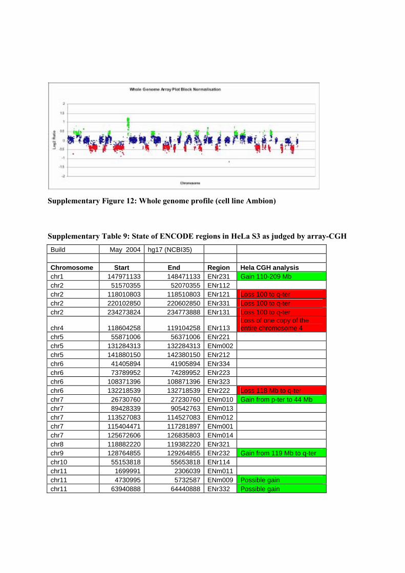
Supplementary Figure 12: Whole genome profile (cell line Ambion)

Supplementary Table 9: State of ENCODE regions in HeLa S3 as judged by array-CGH

Build May 2004 hg17 (NCBI35) Chromosome Start End Region Hela CGH analysis chr1 147971133 148471133 ENr231 Gain 110-209 Mb chr2 51570355 52070355 ENr112 chr2 118010803 118510803 ENr121 Loss 100 to q-ter chr2 220102850 220602850 ENr331 Loss 100 to q-ter chr2 234273824 234773888 ENr131 Loss 100 to q-ter

chr4 118604258 119104258 ENr113 Loss of one copy of the entire chromosome 4

chr5 55871006 56371006 ENr221 chr5 131284313 132284313 ENm002 chr5 141880150 142380150 ENr212 chr6 41405894 41905894 ENr334 chr6 73789952 74289952 ENr223 chr6 108371396 108871396 ENr323 chr6 132218539 132718539 ENr222 Loss 118 Mb to q-ter chr7 26730760 27230760 ENm010 Gain from p-ter to 44 Mb chr7 89428339 90542763 ENm013 chr7 113527083 114527083 ENm012 chr7 115404471 117281897 ENm001 chr7 125672606 126835803 ENm014 chr8 118882220 119382220 ENr321 chr9 128764855 129264855 ENr232 Gain from 119 Mb to q-ter chr10 55153818 55653818 ENr114 chr11 1699991 2306039 ENm011 chr11 4730995 5732587 ENm009 Possible gain chr11 63940888 64440888 ENr332 Possible gain


chr11 115962315 116462315 ENm003 Loss from 88 Mb to q-ter chr11 130604797 131104797 ENr312 Loss from 88 Mb to q-ter chr12 38626476 39126476 ENr123 Gain from 37-54 Mb chr13 29418015 29918015 ENr111 Loss up to 54 Mb chr13 112338064 112838064 ENr132 Gain from 109 Mb to q-ter chr14 52947075 53447075 ENr311 chr14 98458223 98958223 ENr322 chr15 41520088 42020088 ENr233 Gain from 39 Mb to q-ter chr16 0 500000 ENm008 chr16 25780427 26280428 ENr211 chr16 60833949 61333949 ENr313 chr18 23719231 24219231 ENr213 Loss from 18 Mb to q-ter chr18 59412300 59912300 ENr122 Loss from 18 Mb to q-ter chr19 59023584 60024460 ENm007 Loss from 57-59 Mb chr20 33304928 33804928 ENr333 Gain from 30 Mb to q-ter chr21 32668236 34364221 ENm005 chr21 39244466 39744466 ENr133

chr22 30128507 31828507 ENm004Loss of one copy of the entire chromosome

chrX 122507849 123007849 ENr324 Loss from 100 Mb to q-ter chrX 152635144 153973591 ENm006 Loss from 100 Mb to q-ter

CGH analysis was not conducted on additional cell lines beyond the consortium common cell lines. However information is available for other cell lines used from other analyses such as SKY-FISH. HL60 has been mapped by SKY-FISH (data available at http://www.ncbi.nlm.nih.gov/sky/skyquery.cgi - query for HL60) and shows substantial rearrangement82. However it is not possible to precisely determine how these rearrangements affect the ENCODE regions from the SKY-FISH results which are presented by chromosome band. More recent analyses of HL60 are also available83.

S3 Regulation of Transcription

S3.1 ChIP-Chip and ChIP-PET experimental methodology

S3.1.1 Yale Group

S3.1.1.1 Preparation of ChIP DNA from HeLaS3 cells For c-Fos, c-Jun, BAF155 and BAF170 HeLaS3 cells were grown by the National Cell Culture Center in Joklik's modified minimal essential medium (MEM), supplemented with 5% FBS at 37°C in 5% CO2, to a density of 6 x105 cells/ml. Cells were fixed with 1% formaldehyde at room temperature for 10 min and fixation was terminated with 125 mM glycine. The cells were washed twice in cold 1x Dulbecco’s PBS and then stored and shipped as frozen cell pellets. For


STAT1, HeLaS3 cells were grown in Dulbecco's modified Eagle's medium for suspension (SMEM) supplemented with 5% FBS at 37°C in 5% CO2, to a density of 6 x105 cells/ml. The cultures were divided in half and were either induced with 5 ng/ml human recombinant IFN-γ (R&D Systems #285-IF), or left untreated, for 30 min at 37°C, 5% CO2 and then fixed with 1% formaldehyde final concentration at room temperature for 10 min. Fixations were quenched by addition of glycine to 125 mM final concentration and cells were washed twice in cold 1x Dulbecco's PBS. All ChIP DNA samples were isolated from nuclear extracts. Nuclei were prepared by swelling cells for 10 min in hypotonic lysis buffer (20 mM HEPES, pH 7.9, 10 mM KCl, 1 mM EDTA, pH 8, 10% glycerol, 1 mM DTT, 0.5 mM PMSF and protease inhibitors). Following dounce homogenization nuclear pellets were collected and lysed in 1x RIPA buffer (10 mM Tris-Cl, pH 8.0, 140 mM NaCl, 1% Triton X-100, 0.1% SDS, 1% deoxycholic acid, 0.5 mM PMSF, 1 mM DTT, and protease inhibitors). Nuclear lysates were sonicated with a Branson 250 Sonifier to shear chromatin to approximately 0.5 to 1 kb in size. Clarified lysates were incubated overnight at 4°C with factor-specific antibodies. Protein-DNA complexes were precipitated with RIPA-equilibrated protein A agarose beads and immunoprecipitates were washed three times in 1x RIPA, once in 1x PBS, and then eluted from the beads by addition of 1% SDS, 1x TE (10 mM Tris-Cl at pH 7.6, 1 mM EDTA at pH 8), and incubation for 10 min at 65°C. Crosslinks were reversed overnight at 65°C. All samples were purified by treatment first with 200 μg/ml RNase A for 1 h at 37°C, then with 200 μg/ml Proteinase K for 2 h at 45°C, followed by extraction with phenol:chloroform:isoamyl alcohol and ethanol precipitation at -70°C.

S3.1.1.2 Labeling and Hybridization of ChIP DNA samples Full details are available through GEO or are published in Euskirchen et al22. Briefly, for each array to be hybridized ChIP DNA isolated from 1 x 108 cells was directly random primed with Klenow and labeled with either Cy5 (ChIP DNA prepared with a specific antibody) or with Cy3 (reference DNA). The reference DNA samples varied for each factor. For c-Fos and c-Jun, total genomic DNA was used as reference samples. For BAF155 and BAF170 the reference samples were ChIP DNA prepared using normal rabbit IgG. STAT1 ChIP DNA prepared from IFN-γ stimulated cells was compared to STAT1 ChIP DNA prepared from uninduced cells, where STAT1 is nuclear excluded. Labeled ChIP DNA samples were applied to high density oligonucleotide arrays synthesized by maskless photolithography and arrays were hybridized in MAUI hybridization stations (BioMicro Systems) with mixing. Datasets consist of 3 or more biological replicates (defined as ChIP DNA prepared from distinct cell cultures grown, harvested and processed on separate days) and each biological replicate was hybridized to a separate array.

S3.1.1.3 Array Data Processing The array data was processed using the Tilescope tool (tilescope.gersteinlab.org; Zhang et al24). Array data is first quantile normalized and median scaled between replicate arrays (both Cy3 and Cy5 channels). Using a 1000 bp sliding window centered on each oligonucleotide probe, a signal map (estimating the fold enrichment [log2 scale] of ChIP DNA) was generated by computing the pseudo-median signal of all log2(Cy5/Cy3) ratios (median of pairwise averages) within the window, including replicates. Similarly, a P-value map (measuring significance of enrichment of oligonucleotide probes in the window) for all sliding windows was made using the


Wilcoxon paired signed rank test comparing fluorensent intensity between Cy5 and Cy3 for each oligonucleotide probe. A binding site was determined by thresholding oligonucleotide positions with -log10(P-value) (>= 4), extending qualified positions upstream and downstream 250 bp, and requiring 1000 bp space between two sites. The top 200 sites are reported.

S3.1.2 Affymetrix Group

S3.1.2.1 Cell Lines The HL-60 acute myeloid lymphoma cell line was obtained from the American Type Culture Collection facility. Cell were maintained in Iscove's Modified Dulbecco's Medium with GlutaMAX (Invitrogen) containing 20% Fetal Bovine Serum (Invitrogen) and 1X penicillin/streptomycin (Invitrogen) in a humidified 37°C incubator with 5% CO2. For each of the three biological replicates, cultures were seeded at approximately 3x105 cells/ml and were induced with a final concentration of 1 μM all-trans-retinoic-acid (ATRA – purchased from Sigma) after 2 days of growth when cultures had achieved a density of 106 cells/ml. These cultures (3 liters total for each time point) were then incubated for 2, 8, and 32 hours with ATRA or untreated (0 hour) before harvesting. Both cell viability and recovery after ATRA treatment were assessed by Trypan Blue exclusion as well as determining cell density by counting an aliquot on a hemocytometer.

S3.1.2.2 CD11b Cell Surface Antigen Labeling ATRA treated HL-60 cells were monitored for differentiation by detection of CD11b expression. Triplicate samples for each time point in each biological replicate (106 cells per sample) were centrifuged at 300xg for 10 minutes, media aspirated, and resuspended in 100 μl Label Buffer (1x Hanks Buffered Saline, 2% filtered Fetal Bovine Serum, and 0.01% sodium azide). Cells were blocked with 5 μl unlabeled isotype matched mouse IgG1κ (BD Pharmingen) on ice for 15 minutes, then washed with 2 ml ice cold Label Buffer. Cells were pelleted at 300xg for 10 minutes and resuspended in 100 μl Label buffer. Five μl of anti-CDllb antibodies or isotype controlled mouse IgG1κ coupled to Alexa 488 (BD Pharmingen) were added to each sample and incubated on ice for 30 minutes. Cells were washed twice in 2 ml Label Buffer and fixed with 2% formaldehyde in PBS. Samples were stored packed in ice and in the dark until analyzed by flow cytometry using a FACScaliber bench top cell sorter (BD Biosciences) counting 10,000 events for each triplicate sample. IgG1κ labeled samples were used to determine the amount of background fluorescence and non-specific binding. Percent of CD11b positive cells were quantitated using Cellquest Pro software.

S3.1.2.3 Nitroblue Tetrazolium (NBT) Reduction Assay NBT reduction assays were performed in triplicate for each timepoint for each of the 3 biological replicates. Approximately 5x105 were collected by centrifugation at 300xg for 10 minutes at room temperature using a swing bucket rotor. Media was aspirated away and cells were resuspended in 100 μl of growth media. An equal volume of NBT (Roche) diluted 1:50 in PBS was then added to each sample containing 200 ng PMA (Calbiochem). Samples were incubated at 37°C for 30 minutes at which time cells were placed on microscope slides and cells were


scored as either positive or negative based on the presence of dark blue formazin deposites. At least 1000 cells were counted for each of the triplicate samples and percent NBT positive cells was determined for each time point as a measure of differentiation.

S3.1.2.4 RNA preparation Approximately 5x108 cells per time point per biological replicate were harvested by centrifugation and total RNA was purified using RNeasy RNA extraction kit (Qiagen) as per manufacturer’s specifications. Each sample required three columns in order to recover the majority of the RNA. Poly-A RNA was then obtained from the total RNA using Oligo-tex purification kits (Qiagen) as per manufacturer’s instructions.

S3.1.2.5 Formaldehyde Crosslinking and Soluble Chromatin Preparation Cell culture remaining after removing cells for RNA processing was crosslinked using 1% final concentration formaldehyde for 10 minutes at room temperature with gentle swirling. The formaldehyde was quenched using 1/20 culture volume 2.5 M glycine at room temperature for 5 minutes. Cells were pelleted at 500xg for 8 minutes, washed twice with ice cold PBS, and washed three times in Run-on lysis buffer (10 mM Tris pH 7.5, 10 mM NaCl, 3 mM MgCl2, and 0.5% NP40). Recovered nuclei were aliquoted, flash frozen in liquid nitrogen and stored at –80°C until use. Micrococcal nuclease (MNase) digestions were then performed such that there were the equivalent of approximately 2x108 cells per digestion. Frozen pellets were resuspended to a volume of 1.5 ml MNase reaction buffer (10 mM Tris pH 7.5, 10 mM NaCl, 3 mM MgCl2, 1 mM CaCl2, 4% NP40, 1 mM PMSF). Fifteen units of MNase (USB) were added to each reaction, samples were incubated at 37°C for 10 minutes, and the digestion halted by the addition of 30 μl 200 mM EGTA. Forty μl of 100 mM PMSF, 150 μl of protease inhibitors (Roche mini-EDTA free inhibitor pellet resuspended in 500 μl MNase reaction buffer), 200 μl 10% sodium dodecyl sulfate, and 80 μl 5 M NaCl were subsequently added to each reaction. Next, samples were sonicated using a Branson Sonifier-450 four times for 1 minute at a power level setting of 4 and 60% duty. The cellular debris were then cleared by centrifugation on high speed for 10 minutes at 4oC. The supernatant was then removed to a new tube, aliquoted to volumes equivalent to 2x107 cells per tube, flash frozen on liquid nitrogen, and stored at -80°C until use. For each sample, a small aliquot was treated with Pronase, the crosslinks reversed, and run on a 1% TAE-agarose gel to monitor MNase digestion. The average size fragments for each chromatin preparation were 500-1000 base pairs.

S3.1.2.6 Chromatin Immunoprecipitation Chromatin immunoprecipitation were performed using a volume of soluble chromatin equivalent to 2x107 cells. Chromatin was diluted 1:5 using IP Dilution Buffer (20mM Tris pH 8.0, 2mM EDTA, 1% TritonX-100, 150mM NaCl, and Roche mini-EDTA free inhibitor pellet) and pre-cleared with a mix of Protein A (Amersham) and Protein G (Amersham) sepharose beads for 15 minutes at 4°C on a rotator. The pre-cleared diluted chromatin was then incubated with the appropriate amount of antibody of interest overnight at 4°C (see below). Fifty μl of protein A/G mixed sepharose was then added to each IP and incubated for 3 hours at 4oC. IPs were washed in 1 ml Dilution Buffer, centrifuged, the beads resuspended in 0.7 ml Dilution Buffer and


transferred to a Spin-X centrifuge column (Costar). Samples were washed for 5 minutes at room temperature on a rotator using the following buffers respectively: ChIP Wash Buffer 1 (20mM Tris pH 8.0, 2mM EDTA, 1% TritonX-100, 0.1% SDS, 150mM NaCl, 1mM PMSF), ChIP Wash Buffer 2 (20mM Tris pH 8.0, 2mM EDTA, 1% TritonX-100, 0.1% SDS, 500mM NaCl, 1mM PMSF), ChIP Wash Buffer 3 (10mM Tris pH 8.0, 1mM EDTA, 0.25 M LiCl, 0.5% NP-40, 0.5% deoxycholate), and 3 times in TE. Samples were eluted in 200 μl Elution buffer (25mM Tris pH 7.5, 5mM EDTA, 0.5% SDS) at 65°C for 30 minutes. Eluates were collected by centrifugation and an additional 100 ml Elution Buffer was washed through the column. Pronase was added to each sample and to pre-cleared input chromatin samples to a final concentration of 1.5 μg/μl. Samples were incubated at 42°C for 2 hours and at 65°C for at least 6 hours to reverse the crosslinks. Precipitated DNA was then recovered using QIAquick PCR purification columns (Qiagen) as per manufacturer specifications and eluted in 100 μl 10 mM Tris pH 8.5

S3.1.2.7 Antibodies The following antibodies were used per individual IP for the ChIP-Chip experiments: 15 μl anti-tetraacetylated H4 (Upstate 06-866); 3 μg anti-Brg1 (Santa Cruz sc-10768); 3 μg anti-CTCF (Abcam 10571); 12 μl anti-diacetylated H3 (Upstate 06-599); 3 μg anti-Pu.1 (Santa Cruz sc-22805); 3 μg anti-Retinoic acid receptor alpha (Santa Cruz sc-551); 4 μg anti-TFIIB (Santa Cruz sc-225); 4 μg anti-p300 (Santa Cruz sc-584); 4 mg anti-C/EBPε (Santa Cruz sc-158); 3 mg anti-trimethylated H3K27 (a gift from Thomas Jenuwein)

S3.1.2.8 Random Primer Amplification In the first round of amplification (Round A), 30 μl of IP or Input samples, 10 μl dH2O, 12 μl 5X Sequenase Buffer (USB), and 4 μl of 40 μM Primer A (GTTTCCCAGTCACGATCNNNNNNNNN) were mixed in 0.2 ml thin wall PCR tubes. Samples were heated to 95°C for 4 minutes and then flash frozen in liquid nitrogen. The samples were then transferred to 10°C for 5 minutes during which time 0.5 μl 10 mg/ml BSA, 3 μl 0.1 M DTT, 1.5 μl 25 mM dNTPs, and 1.5 μl Sequenase (USB) diluted 1:10 (1.3 U/μl final) were added. Temperature was then raised 1 degree every 20 seconds until it reached 37°C where it was held for an additional 8 minutes. This entire process was then repeated with the exception that only sequence was added during the 5 minutes at 10oC. Next the samples were purified using QIAquick PCR purification columns (Qiagen) as per manufacturer specifications and eluted in 100 μl 10 mM Tris pH 8.5. In the next round of PCR amplification (Round B), 85 μl “Round A” DNA was mixed with 2 μl 100 μM Primer B (GTTTCCCAGTCACGATC) in a standard 100 μl PCR reaction. Samples were then amplified using the following cycler program: 95°C for 3 minutes then 30 cycles of 95°C for 30 seconds, 40°C for 30 seconds, 50°C for 30 seconds, and 72°C for 1 minute. The resulting amplified material was then purified using QIAquick PCR purification columns and eluted in 100 μl 10 mM Tris pH 8.5. One last round of PCR amplification was performed using 90 μl of “Round B” to set up three 300 μl standard PCR reactions using Primer B similar to Round B with the exception that 25 cycles are performed instead of 30 cycles. The three PCR reactions were then combined, purified using 10 QIAquick PCR purification columns, and eluted in a total of 1 ml 10 mM Tris pH 8.5. Eluted samples were precipitated on ice using 1/10 volume NaOAc pH 5.2 and 3 volumes of 100% EtOH.


Precipitated pellets were washed once with 70% EtOH, dried, and resuspended in 40 μl 10 mM Tris pH 8.5.

S3.1.2.9 Microarray Hybridizations and Generation of Maps of Binding Sites The precipitated amplified DNA from the chromatin immunoprecipitation experiments was fragmented with DNAse I to an average size of 100 nucleotides, end labeled with biotin using terminal transferase and hybridized to ENCODE tiling oligonucleotide microarrays (Affymetrix cat. No. 900544) at concentration of 10 μg/ml or 2 μg per array as described earlier25, 56. Arrays were scanned on an in-house made scanner with a laser spot size of 3.5 μm and pixel size of 1 μm. The procedure for generation of binding of sites is described in Ghosh et al84.

S3.1.3 Farnham Data -UC Davis-Farnham lab methods

S3.1.3.1 Chromatin Immunoprecipitation (ChIP) Assays HeLa cells were grown and crosslinked with formaldehyde as previously described85. A complete protocol can be found on our website at http://genomics.ucdavis.edu/farnham/ and in Oberley et al86. A mixed monoclonal antibody against E2F1 (KH20/KH95) was purchased from Upstate Biotechnology Incorporated (Lake Placid, NY), a rabbit polyclonal antibody against MYC (N-202; cat#sc-764x was purchased from Santa Cruz Biotechnology, rabbit IgG (cat# 210-561-9515) was purchased from Alpha Diagnostic, and the secondary rabbit anti-mouse IgG (cat# 55436) was purchased from MP Biomedicals. For analysis of the ChIP samples prior to amplicon generation, immunoprecipitates were dissolved in 50 µl of water, except for input samples that were dissolved in 100 µl. Each PCR reaction mixture contained 2 µl of immunoprecipitated DNA, 1X Taq reaction buffer (Promega, Madison, WI), 1.5 mM MgCl2, 50 ng of each primer, 1.7 U of Taq polymerase (Promega, Madison, WI), 200 µM deoxynucleotide triphosphates (Promega, Madison, WI) and 1 M betaine (Sigma, St, Louis, MO) in a final reaction volume of 20 µl. PCR mixtures were amplified for 1 cycle of 95°C for 5 min, annealing temperature of the primers for 5 min, and 72°C for 3 min followed by 31-33 cycles of 95°C for 1 min, annealing temperature of the primers for 1 min, and 72°C for 1 min and 1 cycle of 72°C for 7 min. PCR products were separated by electrophoresis through 1.5% agarose gels and visualized by ethidium bromide intercalation.

S3.1.3.2 Amplicon Preparation Briefly, two unidirectional linkers oligoJW102 (5’gcg gtg acc cgg gag atc tga att c 3’) and oligoJW103 (5’ gaa ttc aga tc 3’) were annealed and blunt-end ligated to the ChIP samples. Amplicons were created by PCR; each sample consisted of 5 µl 10X Taq polymerase buffer, 7 µl 2mM dNTPs, 3 µl MgCl2, 6.5 µl betaine, 2.5 µl oligoJW102 (20µM), 1 µl Taq (Promega, M1861), and 25 µl of the blunted and ligated chromatin. PCR was run with one cycle at 55°C for 2 min, 72°C for 5 min, and 95°C for 2 min. 15 cycles were then run at 95°C for 0.5 min, 55°C for 0.5 min, and 72°C for 1 min. Finally the products were extended at 72°C for 4 min, then held at 4°C until purified using the Qiaquick PCR purification kit according to the manufacturer’s instructions. 2.5 µl of the first round of amplicons were used as described above to generate a


second round of amplicons. DNA was quantitated and stored -20°C until sent to NimbleGen. For more details, see http://genomics.ucdavis.edu/farnham/ and Oberley et al86.

S3.1.3.3 Array Hybridization High density ENCODE oligonucleotide arrays were created by NimbleGen Systems (Madison, WI, USA) and contained ~380,000 50mer probes per array, tiled every 38 bp. The regions included on the arrays encompassed the 30 MB of the repeat masked ENCODE sequences, representing approximately 1% of the human genome. The labeling of DNA samples for ChIP-chip analysis was performed by NimbleGen Systems, Inc. Briefly, each DNA sample (1 µg) was denatured in the presence of 5'-Cy3- or Cy5-labeled random nonamers (TriLink Biotechnologies, San Diego) and incubated with 100 units (exo-) Klenow fragment (NEB, Beverly, MA) and dNTP mix [6 mM each in TE buffer (10 mM Tris/1 mM EDTA, pH 7.4; Invitrogen)] for 2 h at 37°C. Reactions were terminated by addition of 0.5 M EDTA (pH 8.0), precipitated with isopropanol, and resuspended in water. Then, 13 µg of the Cy5-labeled ChIP sample and 13µg of the Cy3-labeled total sample were mixed, dried down, and resuspended in 40 µl of NimbleGen Hybridization Buffer (NimbleGen Systems) plus 1.5 µg of human COT1 DNA. After denaturation, hybridization was carried out in a MAUI Hybridization System (BioMicro Systems, Salt Lake City) for 18 h at 42°C at the NimbleGen Service Laboratory. The arrays were washed using NimbleGen Wash Buffer System (NimbleGen Systems), dried by centrifugation, and scanned at 5-µm resolution using the GenePix 4000B scanner (Axon Instruments, Union City, CA). Fluorescence intensity raw data were obtained from scanned images of the oligonucleotide tiling arrays using NIMBLESCAN 2.0 extraction software (NimbleGen Systems). For each spot on the array, log2-ratios of the Cy5-labeled test sample versus the Cy3-labeled reference sample were calculated. Then, the biweight mean of this log2 ratio was subtracted from each point; this procedure is approximately equivalent to mean-normalization of each channel. Sites bound by E2F1 and Myc were identified using the peak calling algorithm described in Bieda et al19 and available at http://genomics.ucdavis.edu/farnham/.

S3.1.4 Sanger Group (PCR Arrays) We assayed H3k4me1, H3k4me2, H3k4me3, H3Ac, and H4Ac across ENCODE in both GM06990 cells and Hela S3 cells using a modified chromatin immunoprecipitation followed by microarray read-out (‘chip-on-chip’) procedure16.

S3.1.4.1 Generation of chromatin immunoprecipatation (ChIP) samples Human cell line GM06990 (CEPH/UTAH PEDIGREE 1331) was cultured in RPMI640, 15% fetal calf serum, 1% penicillin-streptomycin and 2 mM L-glutamine. Human cell line HeLa-S3 was cultured in Joklic’s DMEM, 5 % newborn bovine serum by the National Cell Culture Center Minneapolis, USA. 108 cells were collected by centrifugation, resuspended in 50 ml pre-warmed serum free media in a glass flask. Formaldehyde (BDH) was added to final concentrations of 0.37 or 1%. After incubating the cells for 10 minutes with gentle agitation at room temperature, glycine (Sigma) was added to a final concentration of 0.125M followed by again incubating for 5 minutes at RT with agitation. Cells were collected at 4°C, resuspended in 1.5 ml ice-cold PBS and centrifuged at 2000 rpm for 5 min at 4°C (Sorval Heraeus). The cell pellet was resuspended in ~1.5X pellet volume of cell lysis buffer (10mM Tris-HCl pH 8.0, 10mM NaCl, 0.2% Igepal


CA-630, 10mM sodium butyrate, 50µg/ml PMSF, 1µg/ml leupeptin) and incubated for 10 minutes on ice. The cell nuclei were collected by centrifugation at 2500 rpm for 5 minutes at 4°C. The nuclei were resuspended in 1.2 ml of nuclear lysis buffer (NLB 50mM Tris-HCl pH 8.1, 10mM EDTA, 1% SDS, 10mM sodium butyrate, 50µg/ml PMSF, 1µg/ml leupeptin) and incubated on ice for 10 minutes. After adding 0.72 ml of immunoprecipitation dilution buffer (IPDB 20mM Tris-HCl pH 8.0, 150mM NaCl, 2mM EDTA 1% Triton X-100, 0.01% SDS, 10mM sodium butyrate, 50µg/ml PMSF, 1µg/ml leupeptin) the chromatin was transferred to a 5ml tube (falcon) and sheared to a fragment size of ~ 500 bp by sonication (Branson sonifier using settings of time: 8 min, amplitude: 16 %, pulse on 0.5 s, pulse off 2.0 s, 450 digital,). During sonication samples were cooled in an ice water bath. Debris was removed from the sheared chromatin by centrifugation in a cooled bench centrifuge (Eppendorf) at 14000 rpm for 5 minutes at 4°C. The supernatant was diluted with 4.1 ml of IPDB to a final ratio of NLB:IPDB of 1:4. The chromatin was precleared by adding 100µl of normal rabbit IgG (Upstate) and incubating for 1 hour at 4°C on a rotating wheel. 200 µl of homogeneous protein G-agarose suspension was added (Roche) and incubation continued for 3 hours to overnight at 4°C on a rotating wheel. The protein G-agarose was spun down at 3000 rpm for two minutes at 4°C. 1.35 ml of supernatant (chromatin) was used to set up each ChIP assay while 270 µl were used as input control. Ten micrograms of antibody was used in each ChIP assay. Antibodies used were di-acetylated histone H3 (06-599, Upstate), tetra-acetylated histone H4 (06-866, Upstate), histone H3 mono-methyl lysine 4 (ab8895, Abcam), histone H3 di-methyl lysine 4 (ab7766, Abcam), histone H3 tri-methyl lysine 4 (ab8580, Abcam). The chromatin and antibody were incubated on a rotation wheel overnight at 4°C, then 100 µl of homogeneous protein G-agarose suspension was added (Roche) and incubation continued for 3 hours. The protein G-agarose was spun down and the pellet washed twice with 750 µl of IP wash buffer 1 (20 mM Tris-HCl pH 8.1, 50 mM NaCl, 2 mM EDTA, 1% Triton X-100, 0.01% SDS), once with 75 EPAL CA630, 1% deoxycholic acid) and twice with 10 mM Tris-HCl 1 mM EDTA pH80 µl of IP wash buffer 2 (10 mM Tris-HCl pH 8.1, 250 mM LiCl, 1 mM EDTA, 1% IG.0. The immune complexes were twice eluted from the beads by adding 225 µl of IP elution buffer (100mM NaHCO3, 0.1% SDS). After adding 0.2 µl of RNase A (10 mg/ml, ICN) and 27 µl of 5M NaCl to the combined elutions and adding 0.1µl of RNAse A and 16.2 µl of 5M NaCl to the input sample, the samples were incubated at 65°C for 6 hours. Then 9 µl of proteinase K (10 mg/ml, Invitrogen) was added and the samples incubated at 45°C overnight. Immediately before the DNA was recovered using phenol chloroform extraction, 2 µl tRNA (5 mg/ml stock/ Invitrogen) was added. The aqueous layer was extracted once with chloroform. Then 5 µg of glycogen (Roche), 1 µl of tRNA (5 mg/ml Invitrogen), 50 µl of 3M sodium acetate pH 5.2 and 1.25 ml of ice-cold ethanol was added to precipitate the DNA at -20°C over night. The DNA pellets were washed with 70% ethanol, air dried and resuspended in 100 µl of water for input samples and 50 µl of water for ChIP samples.

S3.1.4.2 Fluorescent DNA labeling, microarray hybridization and data analysis Fluorescently labelled DNA samples were prepared using a modified Bioprime labelling kit (Invitrogen) in 150 µl reaction volumes containing 450 ng Input DNA or 40% of ChIP DNA, dNTPs (0.2 mM dATP, 0.2 mM dTTP, 0.2 mM dGTP, and 0.1 mM dCTP), 0.01 mM Cy5/Cy3 dCTP (GE Healthcare) , 60 μl 2.5x random primer solution (750 μg/ml, Invitrogen) and 3 μl of Klenow fragment (Invitrogen) . Input DNA samples were labeled with Cy5, and ChIP DNA samples were labelled with Cy3 over night at 37°C. Labelling reactions were purified using


Micro-spin G50 columns (Pharmacia-Amersham) in accordance with the manufacturer's instructions. Input and ChIP sample were combined and precipitated with 3 M sodium acetate (pH 5.2) in 2.5 volumes of ethanol with 135 µg human Cot DNA (Invitrogen). The DNA pellet was resuspended in 80μl hybridization buffer containing 50% deionized formamide (Sigma), 10 mM Tris-HCl (pH 7.4), 5% dextran sulphate, 2× SSC, 0.1% Tween-20. Two combined labeling reactions were denatured for 10 minutes at 100°C, snap frozen on ice and used for one microarray hybridisation. Microarrays were hybridized on an automatic hybridization station (HS4800, Tecan) for 45h at 37°C with medium agitation, washed 10 times for 1 minute with PBS 0.05% Tween20 (BDH) at 37°C, 5 times for 1 minute with 0.01x SSC at 52°C, 10x 1 minutes with PBS 0.05% Tween20 at 23°C, followed by a final wash with HPLC-grade water (BDH) at 23°C and drying under nitrogen flow for 4 minutes. Microarrays were scanned using a ScanArray 4000 confocal laser-based scanner (Perkin Elmer). Mean spot intensities from images were quantified using ScanArray Express (Perkin Elmer) with background subtraction. Spots affected by dust were manually flagged as “not found” and subsequently excluded from the analysis.

S3.1.4.3 ENCODE tiling array construction The final Encode array spanned 23.8 Mb and contained 24005 array elements (average size 992 bp). Primers pairs used to amplify PCR products for the arrays were designed using primer 3 including repetitive elements where possible. (The primer sequences for amplicons used as array elements are available at ftp://ftp.sanger.ac.uk/pub/encode/microarrays/). In order to generate arrays containing single-stranded array elements, all amplicons used in this study were prepared and printed on arrays as previously described (see Dhami et al87 and www.sanger.ac.uk/Projects/Microarrays/arraylab/methods.shtml). All PCR products were prepared as follows. A 5’-(C6) amino-link was added to all forward primers. The primer pairs (final concentration 0.5 µM) were used to amplify PCR products in a 60-µl final volume PCR containing 50 mM KCl, 5 mM Tris HCl (pH 8.5), 2.5 mM MgCl2, 10 mM dNTPs (Pharmacia), 0.625 U Taq polymerase (Perkin Elmer), and 50 ng of human genomic DNA (Roche). The PCR products were amplified with the following program: 1x 5 min 95°C, 35 x 95°C 1.5 min, 65°C 1.5 min (-0.3°C per cycle), 72°C 3 min, 1x 72°C 5 min. For arraying of PCR products, spotting buffer was added at final concentrations of 0.25 M sodium phosphate buffer pH 8.5 and 0.00025% sodium sarkosyl (BDH). The PCR products were filtered through multiscreen-GV 96-well filter plates (Millipore), aliquoted into 384-well plates (Genetix), and were arrayed onto Codelink slides (GE) in a 48-block format using a Microgrid II arrayer (Biorobotics/Genomic Solutions). Slides were processed to generate single-stranded array elements, as described at http://www.sanger.ac.uk/Projects/Microarrays/, and were stored at room temperature until hybridized.

S3.1.4.4 Data processing for analysis The data of the ratio of the background corrected ChIP signal divided through the background corrected input signal, both globally normalised were used for the HMM analysis. Ratios of duplicated spots were averaged. Ratios of spots defined as “not found” and ratios with a value below zero were excluded from the analysis and also excluded from the median track of technical replicates. Each median track of technical replicates was automatically generated with an individual R script (i.e.


ftp://ftp.sanger.ac.uk/pub/encode/H3K4me3_GM06990_2/H3K4me3_GM06990_2.R) which combines only positive values of technical replicates not classified as “not found”.

S3.1.4.5 Comprehensive annotation of peaks using hidden Markov model analysis A two-state HMM3 was used to analyze the Sanger ChIP-chip data. The states of the HMM represent regions of the tile path corresponding to locations either consistent or inconsistent with antibody binding. The emission probabilities of the states are derived from the probability that a point is part of a normal distribution fitted from the 45% of the data with the lowest enrichment values. The fitted distribution is calculated separately for each of the ENCODE regions using the Levenberg-Marquart curve-fitting technique. The optimal state sequence for the observed data was calculated from the HMM using the Viterbi algorithm. The resulting list of tiles assigned to the state consistent with antibody binding was post-processed to develop a final hit list, which combined positive tiles within 1000bp of each other into “hit regions.” The score of each hit region was determined by taking the summation of the median enrichment values of the tiles in the contiguous portions (i.e. the area under the peak). The center position of the PCR tile with the highest enrichment value in the hit region was deemed the center of the peak.

S3.1.4.6 Identification of significant peaks ( p<0.01 level) For the purposes of our analyses we defined significant peaks as those identified using the approach described above wherein the peak signal exceeded the 99th% confidence bound on outliers relative to the global distribution of each mark. To determine the 99% confidence bound, we analyzed log(2)-transformed microarray signal intensity ratios and computed the 99th percentile of values below log(2)=0. Such ratio values were considered to signify experimental noise. A standard assumption is that this noise is symmetric about the log(2)=0 baseline. We therefore reflected the 99th percentile values about the baseline for each mark. This established an empirical 99% confidence bound on outliers, which is equivalent to a p<0.01 threshold. We then identified, for each histone mark, the HMM-derived signal peaks in which the maximum signal exceeded the p<0.01 level.

S3.1.5 UT Austin ChIP-chip methods

S3.1.5.1 ChIP protocol for c-Myc and E2F4 Briefly, cells were cross-linked by addition of formaldehyde (1 % final concentration) directly to tissue culture plates for 7 min at room temperature. Cross-linking was terminated by adding glycine to a final concentration of 125 mM. Cells were washed with cold phosphate-buffered saline (PBS) containing PMSF, scraped off the plates, collected by centrifugation and washed again. After centrifugation, the pellet was resuspended in SDS lysis buffer (1 % SDS, 10 mM EDTA, 50 mM Tris-Cl pH 8.1, plus protease inhibitors) and incubated at room temperature for 20 min. Cells were sonicated on ice and centrifuged at 12000 rpm at 4 °C for 10 min. 10x ChIP dilution buffer (0.1 % SDS, 1 % Triton X-100, 2 mM EDTA, 20 mM Tris-Cl pH 8.1, 150 mM NaCl, plus protease inhibitors) was added to the collected supernatant. Sample was pre-cleared with protein A-agarose beads (previously washed with 10x ChIP dilution buffer) at 4 °C for 1 hr. Precleared chromatin was incubated with the corresponding specific antibody (anti-e2f4 antibody


sc-1082x, Santa Cruz for E2F4 and anti-myc antibody sc-764x, Santa Cruz for c-Myc) at 4 °C overnight. For the mock IP controls, the antibody was left out. Pre-washed protein A-agarose beads were added and protein-DNA complexes were recovered after a 2 hour incubation at 4 °C. Immunoprecipitated complexes were successively washed with Lowsalt wash buffer (0.1 % Deoxycholate, 1 % Triton X-100, 1 mM EDTA, 50 mM HEPES pH 7.5, 150 mM NaCl), High-salt wash buffer (0.1 % Deoxycholate, 1 % Triton X-100, 1 mM EDTA, 50 mM HEPES pH 7.5, 500 mM NaCl), LiCl wash buffer (250 mM LiCl, 0.5 % NP-40, 0.5 % Deoxycholate, 1 mM EDTA, 10 mM Tris-Cl pH 8.1) and TE buffer (10 mM Tris-Cl pH 7.5, 1 mM EDTA). SDS elution buffer was added and incubated at 65 °C for 30 min to recover protein-DNA complexes. Crosslinks were reversed by incubating at 65 °C overnight. The sample was treated with RNase A and Proteinase K, extracted with phenol:chloroform and precipitated. The pellet was resuspended in 25 μl of water. We used this ChIP DNA for STAGE as well as ChIP-chip.

S3.1.5.2 Hybridization of ChIP DNA to NimbleGen ENCODE arrays ChIP and mock IP DNA samples were amplified and labeled for hybridization essentially using NimbleGen's recommended protocols. DNA was amplified by ligation mediated PCR as previously described14. The ChIP samples were labeled with Cy5 while the mock IP samples were labeled with Cy3 and used as a reference channel in two colour hybridizations. Hybridization was carried out at NimbleGen's service facility (Madison, WI) using their standard procedures. Microarray scanning, data acquisition, normalization and peak finding was done essentially as previously described for NimbleGen arrays14.

S3.1.6 UCSD ChIP-chip methods Three biological replicates of treated and untreated cells were crosslinked and harvested as previously described14 with the following modifications. Cells were crosslinked for 20 minutes at 37ºC in normal culture media plus 1/10 volume formaldehyde crosslinking solution in large culture plates, followed by glycine quenching and PBS wash at room temperature. Crosslinked cells were collected by scraping and centrifugation. Chromatin was isolated and fragmented as previously described14, though generating fragments of 1.5 Kbp in length required 12 x 30 sec cycles of sonication.

S3.1.6.1 Labeling procedure One microgram (μg) of LM-PCR products were used for labeling and hybridization to each array. One microgram of immunoprecipitated or total genomic LM-PCR DNA was mixed with 40 μL of 1 μM Cy5 or Cy3 end labeled random prime nonamer oligonucleotides (TriLink Biotechnologies) respectively with the bacterial label control DNA in a total volume of 88 μL. The DNA and random primers were annealed by heating the sample to 98°C for 5 minutes and chilled quickly in ice water for 2-3 minutes. Two microliter of (100 units) of E. coli DNA polymerase Klenow fragment and 10 μL of 10 mM equimolar mixture of dATP, dTTP, dCTP, and dGTP were added to the annealed DNA sample and incubated at 37°C for 2 hours. The reaction was stopped by addition of 10 μL of 0.5 M EDTA. The labeled sample was ethanol precipitated by addition of 11 μL 5 M NaCl and 110 μL isopropanol. The precipitate was collected by centrifugation and the resulting labeled DNA pellet was washed with 80% ethanol


(V/V). The pellet was dried under vacuum for 5-15 minutes to remove any remaining liquid, and the resulting dry labeled DNA pellet was resuspended in 10 μL dH2O.

S3.1.6.2 Hybridization procedure and parameters Equal amounts (12 μg) of Cy5 and Cy3 labeled DNA samples were mixed, and 4 μL 2.94 nM Xenohybe control oligos (an equimolar mixture of 5＇TTGCCGATGCTAACGACGCATCAGACTGCGTACGCCTAAGCAACGCTA3＇ and 5＇CATTGCTGTGCGTACGCAGTCAAGTCGATCACGCTAACTCGTTGCGAC3＇) was added to the mixture. The sample was vacuum dried under low heat until the volume of sample was less than 14.4 μL. The final volume of DNA was adjusted to 14.4 μL with dH2O. To this sample, 11.25 μL 20X SSC, 18 μL 100% formamide, 0.45 μL 10% SDS, 0.45 μL 10X TE (100mM Tris, 10mM EDTA), and 0.45 μL equimolar mixture of Cy3 and Cy5 labeled CPK6 oligonucleotides (5＇TTCCTCTCGCTGTAATGACCTCTATGAATAATCCTATCAAACAACTCA3＇ and 5＇TTCCTCTCGCTGTAATGACCTCTATGAATAATCCTATCAAACAACTCA3＇, respectively) were added to prepare the hybridization mixture. The hybridization sample was heated to 95 °C and was applied to the slide and incubated in the MAUI® Hybridization Station (BioMicro Systems, Inc.) at 42°C for 16-20 hours. The hybridized slides from the MAUI® Hybridization Station were washed once in Wash 1 (0.2X SSC, 0.2% SDS, 0.1 mM DTT) for 10-15 seconds and followed by another wash in Wash 1 (0.2X SSC, 0.2% SDS, 0.1 mM DTT) for 2 minutes with gentle agitation. The slides were then washed in Wash 2 (0.2X SSC and 0.1mM DTT) for 1 minute and followed by a wash in Wash 3 (0.05X SSC and 0.1 mM DTT) for 15 seconds. The slides were dried by centrifugation

S3.1.6.3 Measurement data and specifications The hybridized arrays were scanned on an Axon GenePix 4000B scanner (Axon Instruments Inc.) at wavelengths of 532nm for control (Cy3), and 635nm (Cy5) for experimental sample. PCR arrays were processed using GenePix 4.0 software while NimbleGen data were extracted from the scanned images using the NimbleScan 2.0 program (NimbleGen Systems, Inc.). The arrays were gridded using the automated gridding algorithm, and extracted in two channels using a mean intensity calculation of the interior of the gridded rectangular features upon extraction, and each pair of N probe signals were converted into a scaled log ratio using the function: R(i) = Log (Experimental(i) / Control(i))

S3.1.7 ChIP-PET method description HCT116 Cells before and after 5-FU treatment were cross-linked with 1 % formaldehyde for 10 min at room temperature. Formaldehyde was inactivated by addition of 125 mM Glycine. Chromatin extracts containing DNA fragments of average size 500 bp were immunoprecipitated using anti-p53 DO1 monoclonal antibody (Santa Cruz Biotechnology). For all ChIP experiments, quantitative PCR analyses were performed in real time using ABI PRISM 7900 Sequence Detection System and SYBR Green master mix as described (Ng et al., 2003). Relative


occupancy values were calculated by determining the apparent immunoprecipitation efficiency (ratios of the amount of immunoprecipitated DNA over that of the input sample) and normalized to the level observed at a control region, which was defined as 1.0. The control region is a 279 bp region on chromosome 22 and is amplified using the following primers: 5’-GGACTCGGAAGAGGTTCACCTTCGG-3’ and 5’-GTCGCCTCCGCTTGCTGAACTCAATGC-3’. ChIP enriched DNA fragments were end-polished and ligated to the cloning vector pGIS3, which contains two MmeI recognition sites. The ligations were transformed into electrocompetent TOP10 bacterial cells to form the ChIP DNA library. Purified plasmid prepared from the ChIP DNA library was digested with MmeI, end-polished with T4 DNA polymerase to remove the 3’-dinucleotide overhangs, and the resulting plasmids containing a signature tag from each terminal of the original ChIP DNA insert were self-ligated to form single-ditag plasmids. These were then transformed into TOP10 cells to form a “single-ditag library”. Plasmid DNA extracted from this library was digested with BamHI to release 50 bp paired end ditags. The PETs were PAGE-purified, then concatenated and separated on 4-20% gradient TBE-PAGE. An appropriate size fraction (1 kb-2 kb) of the concatenated DNA was excised, extracted and cloned into BamHI-cut pZErO-1 (Invitrogen) to form the final ChIP-PET library for sequencing. PET sequences containing 18 bp from 5’ and 18 bp from 3’ ends of the original ChIP DNA fragments were extracted from the raw sequences obtained from the PET library, and mapped to human genome assembly (hg17). The process of PET extraction and mapping is essentially the same as previously described for cDNA analysis32. The specific mapping criteria are that both the 5’ and 3’ signatures must be present on the same chromosome, on the same strand, in the correct orientation (5’→3’), with minimal 17 bp match, and within 4 kb of genomic distance. Based on the genomic coordinates, we took the center point of each PET cluster to measure the distances to the nearest genes on both sides of the cluster. The genes that had a distance from the nearest clusters of ≤ 100 kb were selected. We did not intend to absolutely associate the PET clusters with particular genes, but tried to provide the distance of the clusters to the nearest genes along the chromosomes.

S3.2 STAGE Data Generation Methods The ChIP protocol is described in section S3.1.5.1 Generation of sequence tags from c-Myc ChIP DNA was carried out as described before88. Briefly, DNA was amplified using a biotinylated primer. We then essentially followed the LongSAGE protocol (http://www.sagenet.org/), but using amplified, biotinylated ChIP DNA as the starting material. Amplified DNA (1-2 µg) was digested with NlaIII. The terminal DNA fragments were bound to streptavidin-coated magnetic beads (Dynal) and separated into two tubes. After ligation with linker 1 or 2, which contain recognition sites for MmeI, the DNA fragments were released by MmeI digestion. The released tags were ligated to generate ditags. Ditags were amplified with nested primers, gel purified, and trimmed by NlaIII digestion. Trimmed ditags were gel purified, concatamerized by ligation, and cloned into the pZero 1.0 vector (Invitrogen). Insert sizes were assayed in recombinant clones and clones containing at


least 10 ditags were sequenced. For STAGE analysis of STAT1, we amplified gel purified ditags from an intermediate step of the STAGE protocol using linker specific primers and sequenced the population of ditags directly using bead-based pyrosequencing (454 Inc.). Analysis of STAGE tags was carried out as described in Kim et al88 and Bhinge et al17.

S3.3 DNaseI sensitivity and hypersensitivity: Data generation and analysis

S3.3.1 Mapping of DNaseI hypersensitivity sites with Quantitative Chromatin Profiling

DNaseI hypersensitive sites were mapped in ENCODE regions by applying the Quantitative Chromatin Profiling (QCP) methodology4 to the following cell types: GM06990, HelaS3, CACO2, and SKnSH (all regions); K562, primary fetal and adult erythroblasts (ENm009); HepG2 and Huh7 (ENm003); PANC1, Calu3, primary large and small airway cells (ENm001); primary CD4 (ENm002). DNaseI sensitivity ratios were obtained for ~118,000 PCR amplicons (avg. length ~225bp) tiled end-to-end across the ENCODE regions. The tiling path covered approximately 86% of ENCODE sequence, encompassing all unique sequence and a large fraction of RepeatMasked sequence. DNaseI hypersensitive sites (DHSs) were identified by computing a moving baseline using a LOESS approach; determining the 95% confidence bound relative to the moving baseline; and identifying outliers (=DHSs).

S3.3.2 Mapping of DNaseI sensitivity and hypersensitivity with DNase/Array DNaseI sensitivity and DHSs were mapped across ENCODE regions in GM06990 and HeLa S3 cells using the DNase/Array methodology5. We cultured cells using standard protocols. To remove background introduced from actively dividing cells, we synchronized cells in G1 by sequential temperature shifts. Cells were placed on ice for 1hr prior to nuclear harvest. We performed nuclear extraction, permeabilization, and DNaseI (Roche, Indianapolis, IN) digestions using a standard approach as described previously in Dorschner et al4. To isolate chromatin-specific and non-specific DNaseI fragments, we size fractionated both the control and treated samples using sucrose step gradients. We pooled fractions with fragments smaller than 1.5kb and cleaned the DNA using Qiagen (Valencia, CA) PCR purification columns according to the manufacturer’s protocol. Samples were labeled and hybridized to a Nimblegen DNA microarray comprising ~390,000 50-mer probes tiled with 12-bp overlap across non-RepeatMasked regions of the ENCODE regions. DHSs were identified as peaks in the signal ratio that exceeded the P<0.01 level = 99th percent confidence bound on outliers. Results were extensively validated using conventional DNaseI sensitivity assays.

S3.3.3 Mapping of DNaseI hypersensitive sites with DNase-chip DNaseI hypersensitive sites and DNaseI sensitivity were mapped across ENCODE regions with the DNase-chip methodology2.

S3.3.3.1 Preparation of DNase treated nuclei for DNase-chip Intact nuclei were isolated from GM06990 and Hela S3 cells using methods previously described2. Nuclei from 3 biological replicates were digested with 3 different optimized concentrations of DNaseI. We blunt ended the DNase digested fragments using T4 DNA polymerase. Genomic DNA used for the random sheared reference control was purified from


each cell line (Gentra), vigorously pipetted and vortexed to generate randomly sheared DNA fragments, and blunt ended.

S3.3.3.2 Capture of DNase digested ends for DNase-chip We ligated biotinylated linkers (5’ Biotin-GCG GTG ACC CGG GAG ATC TGA ATT C and 5’ Phos-GAA TTC AGA TC-3AmM) to DNase digested ends from DNase treated or randomly sheared DNA. The ligation mix was sonicated to generate 200-500 base pair fragments, and biotin-labeled fragments were enriched using streptavidin-coated magnetic beads (Dynal). The sonicated ends were made blunt using T4 DNA polymerase and ligated to nonbiotinylated linkers described above. The DNase captured material was amplified using ligation mediated PCR (5’ GCG GTG ACC CGG GAG ATC TGA ATT C).

S3.3.3.3 Hybridization to tiled ENCODE microarrays and data analysis for DNase-chip We labeled ligation mediated PCR products from DNase treated and random sheared DNA with Cy3- and Cy5-dUTP. Labeled samples were mixed, supplemented with a blocking cocktail (tRNA, Cot1 DNA, Poly A+ RNA, and Poly T+ RNA), and hybridized to Nimblegen ENCODE tiled arrays for >20 hours (Maui). The ENCODE array has approximately 385,000 x 50mer oligos spaced approximately every 38 base pairs of unique sequence (NimbleGen). Slides were washed, scanned (Agilent), and signals were normalized using Nimblescan software. We averaged normalized ratio data (DNase:random) from 9 hybridizations (3 DNase concentrations and 3 biological replicates). We used the ratios to perform a chi-square test on sliding 500 base pair windows to identify regions with a higher than expected number of oligos in the top 5% of the log-ratio distribution (p-values <0.001). Analysis software was written in R (http://www.r-project.org) and is available upon request.

S3.3.4 Generation of a common set of DHS for GM06990 lymphoblastoid cells When applied to the same tissue type, the aforementioned methodologies have considerable overlap. Because the cell preparation procedures differ amongst the method, and because of minor intrinsic biological variability between preparations of the same cell type using the same methodology, some DHSs may be detected in one data set that are not present in the others. We therefore generated a common set of DHSs from lymphoblastoid cells (see section S3.3.5 ). First, thresholded all the individual DHS data sets at the P<0.01 level (i.e., we did not consider DHSs that did not contain signal or indensity ratios that exceeded their respective 99th percent confidence bound on outliers. We next performed a merging step in which overlapping DHSs were merged. In cases where two DHSs in the common data set might be separated by less than 200bp (approximately the size of a nucleosome plus linker DNA), these were merged into a single site.

S3.3.5 Table in supplemental Excel streadsheet This table is included in the attached Excel spreadsheet on the worksheet labeled Section S3.3.5.


S3.4 FAIRE Data Generation methods Formaldehyde Assisted Isolation of Regulatory Elements (FAIRE) was performed in foreskin fibroblast cells (CRL-2091). Cells were grown to 90% confluence in 245 x 245 mm plates and fixed in 1% formaldehyde at room temperature for 1, 2, 4, or 7 minutes. Glycine was added to a final concentration of 125 mM, the cells were spun down at 2K rpm for 4 minutes, and washed twice with cold 1 X PBS containing 100 mM phenylmethylsulphonylflouride. Cells were resuspended in 1 ml of lysis buffer (2% Triton X-100, 1% SDS, 100 mM NaCl, 10 mM Tris-Cl (pH 8.0), and 1mM EDTA) for every 0.1 g of cells and subjected to five 1-minute sessions of glass bead disruption with 2 minutes on ice between sessions. The extract was then sonicated for five sessions of 60 pulses (1 second on/1 second off, 15% amplitude), cooled for 2 minutes on ice between sessions. This yielded an average fragment size of 500 bp. The extract was spun at 15K rpm for 1 minute to clear cellular debris. An equal volume phenol/chloroform was added to the supernatant, vortexed, and spun at 15K rpm for 5 minutes. The aqueous phase was recovered and an additional extraction was performed by adding 1 ml of TE to the organic phase, vortexing, and spinning at 15K rpm for 5 minutes. An equal volume of phenol/chloroform was then added to the pooled aqueous sample, vortexed, and spun at 15K rpm for 5 minutes. Sodium acetate was added to the to a final concentration of 0.3 M. 2X volumes of 95% ethanol was added and incubated at -20°C overnight. The precipitated DNA was pelleted at 15K rpm for 5 minutes, washed with 70% ethanol, and pelleted. The DNA was dried in a speed-vac, resuspended in water, and were incubated at 65°C overnight. 2 μl of RNase A (100 μg/ml) was added and incubated at 37°C for 30 minutes. DNA fragments recovered from the aqueous phase were amplified by ligation-mediated PCR, fluorescently labeled, and hybridized to high-density tiling arrays (NimbleGen Inc., Madison, WI), which cover the non-repetitive portion of the ENCODE regions at 38 bp resolution. A more detailed description of the protocol and subsequent data analysis can be found in Giresi et al3.

S3.5 Generation and categorization of 5' end clusters One of the goals within the ENCODE projects is to find 5' ends of genes and thereby the core promoter regions. The dataset described above and recent studies89 indicates that 5' ends of genes in many cases cannot be described as a single nucleotide position, but a cluster of closely located positions. There are many ways of defining such TSS clusters. In our approach we started with two sets of 5' sites, those identified as the 5' ends of transcripts in the GENCODE annotation (ftp://genome.imim.es/pub/projects/GENCODE/data/TSS_to_share/GENCODE_all_TSS.gff) and those identified by either the CAGE or PET 5' end tag capture technologies (http://genome.ucsc.edu/encode/encode.hg17.html tables encodeGisRnaPetHCT116.bed, encodeGisRnaPetMCF7.bed, encodeGisRnaPetMCF7Estr.bed, encodeRikenCageMinus.bed, encodeRikenCagePlus.bed). In each set, sites located within 60 bp of each other and on the same strand were clustered. The 60 bp criterion was based on analyzing the distribution of distances between 5' end positions from the 5' and 3' map described above. Specifically, we investigated the distances between consecutive nucleotides labeled as TSS on the same strand by any of the


methods. The growth of the cumulative distribution of such distances drop rapidly at around 50-70 nts (see Supplementary Figure 13).

Supplementary Figure 13: Cumulative distribution of the shortest distances between consecutive nucleotides inferred as TSS on the same strand by GENCODE, CAGE and/or PETs. The Y axis shows the fraction of the whole population of distances that are <= x nucleotides

A single genomic coordinate was chosen to represent each cluster. For the GENCODE sites this was the most 5' site in the cluster and for the tag sites it was the site with the highest number of individual tags. There were 1730 GENCODE clusters and 6045 tag clusters. The two sets of clusters were merged and categorised roughly in order of confidence, by determining what type of annotated genomic feature supported their validity. A TSS cluster was considered supported if it lay within the interval +/- 100bp of the given feature. Category A comprised all the GENCODE 5' site clusters. Category B comprised those tag clusters supported by the 5' end of GENCODE exons (ftp://genome.imim.es/pub/other/GENCODE/data/havana-encode/version02.2_14oct05/CHR_coord_hg17/global_files/44regions_CHR_coord.gtf.gz origin in 'VEGA_Antisense_val', 'VEGA_Known','VEGA_Novel_CDS','VEGA_Novel_transcript_val', 'VEGA_Putative_val') on the same strand as the tag cluster but not supported by Category A clusters. Category C comprised those tag clusters not in the previous categories and supported by GENCODE exons on the opposite strand. Category D comprised those tag clusters not in the previous categories and supported by any TxFrag (http://transcriptome.affymetrix.com/download/ENCODE/HS_v35/genes_transcripts/TARs_tran


sfrags/union_TARs_transfrags.bed) or RxFrag (ftp://genome.imim.es/pub/projects/GENCODE/data/RxFrags/suppl_info/). Category E comprised those tag clusters not in the previous categories and supported by a CpG island (http://genome.ucsc.edu/encode/encode.hg17.html table cpgIslandExt) and Category F comprised the remaining, unsupported tag clusters. The Pvalue of the overlap between the Tag data and the supporting data was calculated using overlap statistics based on the Genome Structure Correction method (see Supplement S1.3 ).

S3.5.1 Correlation of Singleton Tag clusters to other transcriptional evidence. The Transcription Start Sites (TSSs) defined by CAGE or DiTags can be defined by one or tags. Any technical false tags, or low level, random transcription is likely to provide single tag TSSs. To assess whether the classifications of TSSs in different evidence catagories were inflated by the presence of random, singleton tags, we repeated the statistical analysis of the overlap (within 100bp, as for the global tag set) between only singleton Tag clusters and each source of supporting evidence. The Table below shows the P-value of seeing the evidence overlap by chance, using the GSC statistic (see Supplement S1.3 ) which conservatively handles heterogeneous distributions in the genome.

Supplementary Table 10: Correlation of singleton tag clusters to other transcriptional evidence

Evidence Type P-value to singleton clusters Sense GENCODE exon 1e-273 Antisense GENCODE exon 1e-95 TxFrag or RxFrag 1e-263 CpG island 1e-313 As the table shows, there is no evidence to support the hypothesis that most of the singleton clusters are randomly distributed around the genome with respect to any of these four classifications of evidence.

S3.6 ChIP enrichment profiles for TSSs These plots show the curves in Figure 5 individually and without smoothing. The x-axis is the relative distance to the nearest anchor (either TSSs or DHSs). The y-axis is the averaged ChIP signal at a certain distance to all anchors. For each plot the signal was first normalized with a mean of 0 and standard deviation 1. The signal of each probe in the ChIP-chip dataset was assigned a distance to its nearest anchor of a given class. Then all signals at the distance to all the anchors were averaged. In order to examine the significance of differences in signal intensity between positions proximal versus distal to anchors, P-values were calculated from two-sided Student's t-test between intensity of all probes within 10Kb range from any anchor and those within 1Kb range, or between outside 5Kb and within 1Kb.


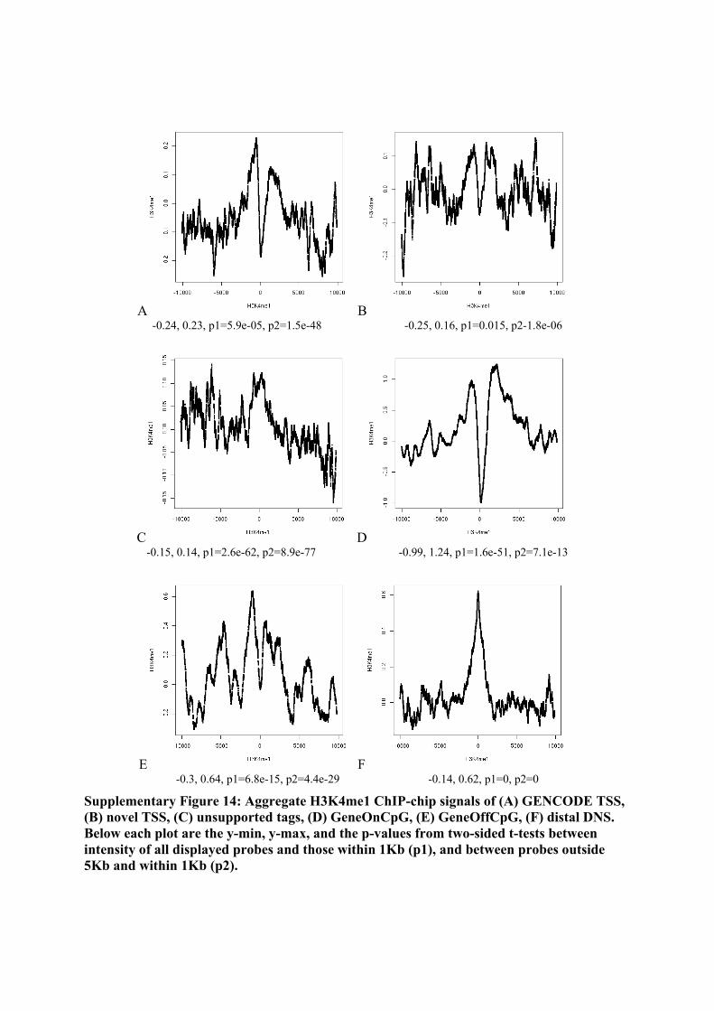
A B -0.24, 0.23, p1=5.9e-05, p2=1.5e-48 -0.25, 0.16, p1=0.015, p2-1.8e-06

C D -0.15, 0.14, p1=2.6e-62, p2=8.9e-77 -0.99, 1.24, p1=1.6e-51, p2=7.1e-13

E F -0.3, 0.64, p1=6.8e-15, p2=4.4e-29 -0.14, 0.62, p1=0, p2=0

Supplementary Figure 14: Aggregate H3K4me1 ChIP-chip signals of (A) GENCODE TSS, (B) novel TSS, (C) unsupported tags, (D) GeneOnCpG, (E) GeneOffCpG, (F) distal DNS. Below each plot are the y-min, y-max, and the p-values from two-sided t-tests between intensity of all displayed probes and those within 1Kb (p1), and between probes outside 5Kb and within 1Kb (p2).


A B -0.27, 0.71, p1=0, p2=0 -0.32, 0.47, p1=0, p2=0

C D -0.15, 0.21, p1=6.1e-32, p2=8.3e-33 -0.31, 3.87, p1=0, p2=0

E F -0.23, 1.82, p1=1.7e-107, p2=3.5e-157 -0.18, 0.41, p1=1.2e-144, p2=7.7e-128



A B -0.25, 0.8, p1=0, p2=0 -0.26, 0.39, p1=1.3e-286, p2=0

C D -0.12, 0.15, p1=3e-06, p2=1.6e-12 -0.33, 4.91, p1=0, p2=0

E F -0.31, 1.32, p1=6e-67, p2=3.9e-90 -0.17, 0.2, p1=7.6e-05, p2=1.2e-16



A B -0.25, 0.85, p1=0, p2=0 -0.38, 0.58, p1=0, p2=0

C D -0.14, 0.15, p1=8.3e-49, p2=3.4e-62 -0.01, 3.95, p1=0, p2=0

E F -0.09, 1.59, p1=6.3e-87, 6.3e-119 -0.21, 0.31, p1=8.1e-107, p2=3.5e-68

Supplementary Figure 17: Aggregate H3ac ChIP-chip signals of (A) GENCODE TSS, (B) novel TSS, (C) unsupported tags, (D) GeneOnCpG, (E) GeneOffCpG, (F) distal DNS. Below each plot are the y-min, y-max, and the p-values from two-sided t-tests between intensity of all displayed probes and those within 1Kb (p1), and between probes outside 5Kb and within 1Kb (p2).


A B -0.2, 0.49, p1=0, p2=0 -0.22, 0.36, p1=1.5e-250, p2=0

C D -0.14, 0.15, p1=2.3e-17, p2=5.5e-21 -0.29, 2.58, p1=0, p2=0

E F -0.23, 0.9, p1=1.9e-38, p2=3e-49 -0.14, 0.21, p1=1.7e-43, p2=1.2e-41

Supplementary Figure 18: Aggregate H3ac ChIP-chip signals of (A) GENCODE TSS, (B) novel TSS, (C) unsupported tags, (D) GeneOnCpG, (E) GeneOffCpG, (F) distal DNS. Below each plot are the y-min, y-max, and the p-values from two-sided t-tests between intensity of all displayed probes and those within 1Kb (p1), and between probes outside 5Kb and within 1Kb (p2).


A B -0.19, 0.58, p1=3.4e-160, p2=9e261 -0.15, 0.32, p1=1e-81, p2=1.8e-112

C D -0.09, 0.16, p1=3.3e-20, p2=2.6e-37 -0.12, 2.55, p1=5.5e-199, p2=5.3e-290

E F -0.21, 0.82, p1=1.2e-33, p2=1.5e-50 -0.13, 0.44, p1=8.6e-68, p2=9.3e-78

Supplementary Figure 19: Aggregate FAIRE signals of (A) GENCODE TSS, (B) novel TSS, (C) unsupported tags, (D) GeneOnCpG, (E) GeneOffCpG, (F) distal DNS. Below each plot are the y-min, y-max, and the p-values from two-sided t-tests between intensity of all displayed probes and those within 1Kb (p1), and between probes outside 5Kb and within 1Kb (p2).


A B -0.15, 0.85, p1=0, p2=0 -0.13, 0.38, p1=5.2e-164, p2=1.2e-296

C D -0.11, 0.19, p1=2.9e-16, p2=1.8e-10 -0.16, 4.37, p1=0, p2=0

E F -0.2, 1.31, p1=2.9e-63, p2=1.7e-105 -0.1, 0.35, p1=4.7e-45, p2=6e-50

Supplementary Figure 20: Aggregate DNAseI signals of (A) GENCODE TSS, (B) novel TSS, (C) unsupported tags, (D) GeneOnCpG, (E) GeneOffCpG, (F) distal DNS. Below each plot are the y-min, y-max, and the p-values from two-sided t-tests between intensity of all displayed probes and those within 1Kb (p1), and between probes outside 5Kb and within 1Kb (p2).


A B -0.06, 0.49, p1=3.9e-07, p2=3.7e-13 -0.12, 0.68, p1=2.8e-11, p2=1.6e-24

C D -0.13, 0.25, p1=0.0074, p2=0.001 -0.01, 0.4, p1=0.005, p2=0.0071

E F 0.13, 0.71, p1=0.041, p2=0.012 -0.16, 0.71, p1=3.7e-10, p2=1.4e-12

Supplementary Figure 21: Aggregate CTCF ChIP-chip signals of (A) GENCODE TSS, (B) novel TSS, (C) unsupported tags, (D) GeneOnCpG, (E) GeneOffCpG, (F) distal DNS. Below each plot are the y-min, y-max, and the p-values from two-sided t-tests between intensity of all displayed probes and those within 1Kb (p1), and between probes outside 5Kb and within 1Kb (p2).


A B -0.14, 0.81, p1=0, p2=0 -0.16, 0.5, p1=1.4e-293, p2=0

C D -0.11, 0.18, p1=4.8e-25, p2=4.9e-25 -0.06, 3.46, p1=0, p2=0

E F -0.06, 1.52, p1=1.8e-72, p2=1.6e-95 -0.17, 0.38, p1=5.8e-79, p2=2.5e-77

Supplementary Figure 22: Aggregate cMyc ChIP-chip signals of (A) GENCODE TSS, (B) novel TSS, (C) unsupported tags, (D) GeneOnCpG, (E) GeneOffCpG, (F) distal DNS. Below each plot are the y-min, y-max, and the p-values from two-sided t-tests between intensity of all displayed probes and those within 1Kb (p1), and between probes outside 5Kb and within 1Kb (p2).


A B -0.22, 1.14, p1=0, p2=0 -0.28,0.74, p1=0, p2=0

C D -0.09, 0.13, p1=3.9e-06, p2=2.6e-05 -0.14, 4.79, p1=0, p2=0

E F -0.12, 2.18, p1=1.6e-124, p2=1.8e-162 -0.22, 0.19, p1-5.8e-60, p2=4.1e-107

Supplementary Figure 23: Aggregate E2F1 ChIP-chip signals of (A) GENCODE TSS, (B) novel TSS, (C) unsupported tags, (D) GeneOnCpG, (E) GeneOffCpG, (F) distal DNS. Below each plot are the y-min, y-max, and the p-values from two-sided t-tests between intensity of all displayed probes and those within 1Kb (p1), and between probes outside 5Kb and within 1Kb (p2).


A B -0.12, 0.44, p1=1.9e-157, p2=6e-263 -0.13, 0.35, p1=3.2e-155, p2=5.3e-294

C D -0.09, 0.12, p1=8.4e-05, p2=1.3e-09 -0.2, 1.31, p1=5.6e-107, p2=7.2e-128

E F -0.18, 0.7, p1=6.1e-25, p2=4.8e-25 -0.21, 0.18, p1=3.3e-31, p2=5.4e-44

Supplementary Figure 24: Aggregate E2F4 ChIP-chip signals of (A) GENCODE TSS, (B) novel TSS, (C) unsupported tags, (D) GeneOnCpG, (E) GeneOffCpG, (F) distal DNS. Below each plot are the y-min, y-max, and the p-values from two-sided t-tests between intensity of all displayed probes and those within 1Kb (p1), and between probes outside 5Kb and within 1Kb (p2).


A B -0.12, 1.03, p1=0, p2=0 -0.21, 0.98, p1=0, p2=0

C D -0.21, 0.13, p1=5.5e-40, p2=3.7e-75 0.04, 1.72, p1=1.3e-212, p2=7.2e-226

E F 0.05, 1.89, p1=3.6e-103, p2=1e-126 -0.3, 0.16, p1=9e-165, p2=6.5e-246

Supplementary Figure 25: Aggregate BAF155 ChIP-chip signals of (A) GENCODE TSS, (B) novel TSS, (C) unsupported tags, (D) GeneOnCpG, (E) GeneOffCpG, (F) distal DNS. Below each plot are the y-min, y-max, and the p-values from two-sided t-tests between intensity of all displayed probes and those within 1Kb (p1), and between probes outside 5Kb and within 1Kb (p2).


A B -0.22, 0.48, p1=1.6e-155, p2=3e-253 -0.16, 0.22, p1=2e-85, p2=2.4e-159

C D -0.12, 0.18, p1=0.00076, p2=3.1e-07 -0.31, 2.8, p1=1.4e-238, p2=0

E F -0.33, 0.32, p1=8.4e-15, p2=2.1e-20 -0.14, 0.24, p1=2.8e-08, p2=0.055

Supplementary Figure 26: Aggregate RNA PolII ChIP-chip signals of (A) GENCODE TSS, (B) novel TSS, (C) unsupported tags, (D) GeneOnCpG, (E) GeneOffCpG, (F) distal DNS. Below each plot are the y-min, y-max, and the p-values from two-sided t-tests between intensity of all displayed probes and those within 1Kb (p1), and between probes outside 5Kb and within 1Kb (p2).


S3.7 Symmetrical Signal Analysis All of the ChIP-chip analysis shows binding peaks both upstream and downstream of features such as the transcription start sites. These binding patterns are not exactly symmetrical on each side of the features, but there does not appear to be a preference for the upstream side of the TSS. In an effort to determine if this effect is an artifact of the array platform or of the analysis, we first assume that the DNA is sheared randomly with respect to the location of the DNA-protein complex. We also assume that the antibodies used do not preferentially pull down sheared fragments in which the DNA-protein binding complex is located on either the 5` end or the 3` end of the fragment. If these assumptions hold, the population of labeled DNA fragments to be hybridized to the tiling array can be considered a random distribution centered on the site of the DNA-protein binding site. There may still be some unintended directional bias if the TSSs considered in each of the categories are biased with respect to the position of the tiles. For example, TSS positions that are biased to the 3’ end of the array tiles will, on average, result in a higher enrichment signal in tiles that are further downstream from the center tile. Similarly, if the TSS positions are located in gaps on the tile path and the positions of the TSSs within the gaps are preferentially toward the 5’ or 3’ end of the gap on the tile path, there will be an enrichment bias to the 3’ or 5’ the DNA-protein binding location, respectively. Supplementary Figure 27 shows that the distribution of the distance of the category A TSSs from the center of the tiles on the Sanger PCR array as a fraction of the tile length is essentially flat. We do note that there is a small bias for category A TSSs to be toward the 3’ end of the tiles and category B TSS- to be toward the 5’ end of tiles. Indeed, the tendency for enrichments to be slightly shifted 3’ appears in Figure 5 and section S3.6 but does not affect the symmetrical nature of the enrichment signatures.


Supplementary Figure 27: Distribution of the distance of category A TSSs from the center of the array tile on the Sanger PCR array platform as a fraction of the total length of the tile.

S3.8 BAF Analysis

S3.8.1 Computational Analysis Both the BAF and CTCF signal show broad enrichment and depletion in aggregate around different positions in the genome. This could be due to a number of different phenomena; for example, enrichment could either be due to a general raising or lowering of the genomic background or due to more specific highly enriched regions near the sites. Broad depletion signals are more complex to understand; as aggregation takes normalised scores, this could be due to a shift in the overall mean signal due to a long tail of highly enriched sites, or a more general shift in the analysis. To characterise this further, we considered the BAF155 signal partitioned into different genomic regions based on the following hierarchy; within 100bp of a Category A TSS, within 5KB of a Category A TSS, within a Gene extent (but outside of the TSS neighborhood), within 1KB of a distal DHS or intergenic. These are plotted in Supplementary Figure 28. The two gene centric regions have their entire distribution right shifted, with very few positions showing low BAF


signal in the close to TSS position (red) and an even distribution of the positions showing enriched BAF (blue) near TSSs. This suggests that the main features of the BAF signal is due to a broad region around each TSS having considerable enrichment across all tiles; this consequently raises the average mean position. The gentle depletion of BAF around distal sites is a more complex story (magenta curve vs black curve). A shift of the mean signal due to the enrichment around the TSS should give a reasonably flat depletion (without a peak) across distal sites. Although broad, the depletion does have a mode around the central site. This is either due to genuine low enrichment cases concentrated at this position (31% of the distal DHS probes are in the lowest quartile of the overall distribution whereas 39% of the intergenic probes), but also could be due to clustering effects of unrecognized TSSs, meaning that sites which are at least 5KB from any detected TSS are also more likely to be distant from undetected TSSs. Aggregate depletion of signal is hard to explain with simple models for the main Chip/Chip distribution being due to random, non biological variables and clearly these signals suggest a more complex view of Chip/Chip data with many biological variables influencing the signal readout across every tile.

Supplementary Figure 28: BAF signal near different classes of genomic feature. Red is within 100bp of a TSS, blue within 5kb of a TSS, green within gene extents, magenta within 1kb of a distal DHS, and black intergenic.

S3.8.2 Sheared chromatin This gel image in Supplementary Figure 29 displays sheared chromatin that was prepared from unstimulated HeLaS3 cells and used in BAF155 and BAF170 ChIP-chips (sample lanes 1 to 3,


with each lane containing a separate biological replicate). For comparison, lanes 4 and 5 show sheared chromatin that was prepared from interferon gamma-stimulated HeLaS3 cells and used in Stat1 ChIP-chips, a transcription factor characterized to have a point source binding profile.

Supplementary Figure 29: Sheared chromatin used in BAF155, BAF170, and STAT1 ChIP Experiments

S3.9 Prediction of TSS activity from chromatin modifications An SVM was used to predict the transcriptional state of the last exon in HeLa and GM06990 cells based on the presence of various histone modifications. The SVM input data set contains individual training patterns labeled as positive or negative according to the assayed activity of transcripts measured by the activity of internal exons from the Affymetrix tiling arrays. Each pattern is a vector of individual measurements from five histone modification assays: H3K4me1, H3K4me2, H3K4me3, H3ac, H4ac. The data set is comprised of 529 patterns, of which 231 are negative and 298 are positive. The performance of the SVM is measured using 10-fold cross-validation. This procedure involves splitting the data set at random into 10 equally sized parts. During each step of cross validation, the SVM is trained on 90% of the data, and the resulting classifier is evaluated on the remaining 10%. To compute the final accuracy, the predictions for all ten test sets are combined. The SVM uses a radial basis kernel function . The width parameter \gamma as well as the SVM soft margin parameters C are selected via internal cross-validation within each training set, considering and . The SVM produced an accuracy of 88% for HeLa, and 91% for GM06990.


S3.10 RFBR Identification Methods

S3.10.1 Identification of RFBRs in ChIP-chip experiments All pre-processing steps were performed using existing methods (normalizeWithinArrays, normalizeBetweenArrays, lmFit, and eBayes) from the R package limma in Bioconductor90. After scanning and image extraction, Cy5 (ChIP DNA) and Cy3 (input) signal values were normalized within each array by applying either intensity-dependent Loess correction based on control probes or median-scaling normalization. To combine replicates, we used quantile-normalization between arrays and a linear model-fitting strategy to estimate an average log-ratio for each probe. For NimbleGen platform arrays, we used a computational peak-finding strategy called MPeak which models binding profiles as triangles with peaks at binding sites, estimates a P-value for significance based on the average of the probe signals defining the triangle, and adjusts the P-value cutoff for multiple-testing by False Discovery Rate (FDR) control91. We applied MPeak on the average profile over replicates, as well as on individual array experiments. To define binding sites, we selected significant peaks at 1, 5, and 10% FDR predicted in the average profile that are supported by peak predictions (at the same FDR) in at least 2 out of 3 replicates. For PCR arrays, a variation on the single-array error model was used to define PCR probes as significantly enriched92. Instead of assuming a standard normal distribution for the test statistics representing the PCR probes, we used the R package locfdr to estimate the parameters of the normal distribution which best fit the middle range of the test statistics93-95. We used this estimated distribution to assign P-values and FDR values for the test statistics based on individual array experiments and for the weighted-average test statistics based on combinations of replicate array experiments. To define enriched binding regions, we selected PCR probes at less than 1, 5, 10% FDR based on their weighted-average test statistics which are also defined as enriched in 2 out of 3 replicates based on P-value <0.01 for the UCSD PCR arrays and P-value <0.05 for the Sanger PCR arrays. For both array platforms, binding sites within 1 kb of each other were combined to define binding regions. The midpoint of each binding region was then used to define a “point-source” binding peak. For Affmetrix platform, differential behavior at four time points (0, 2, 8 and 32 hrs after treatment) was assessed by a modification of Significance Analysis of Microarrays (SAM)96, 97.

S3.10.2 RFBR Identification in ChIP-sequencing experiments Human cancer cell HCT116 and HeLa lines were cultured in DMEM containing 10% FCS and subjected to 5-FU and IF-g treatment followed by cross-linking and chromatin-immunoprecipitation using anti-p53 DO1 monoclonal antibody (Santa Cruz) and anti-STAT1 antibody, respectively. The end polished ChIP DNA fragments were ligated to the cloning vector pGIS3, which contains two MmeI recognition sites to form the ChIP DNA library. Purified plasmid prepared from the ChIP DNA library was digested with MmeI, end-polished with T4 DNA polymerase to remove the 3'-dinucleotide overhangs, and the resulting plasmids containing a signature tag from each terminal of the original ChIP DNA insert were self-ligated to form the


single-ditag library. 50 bp paired end ditags (PETs) were released by BamHI digestion, PAGE-purified, then concatenated and separated on a 4-20% gradient TBE-PAGE. An appropriate size fraction (1-2 kb) of the concatenated DNA was excised, extracted and cloned into BamHI-cut pZErO-1 (Invitrogen) to form the final ChIP-PET library for sequencing. PET sequences containing 18 bp from 5' and 18 bp from 3' ends of the original ChIP DNA fragments were extracted from the raw sequences obtained from the PET library, and mapped to human genome assembly hg17. The process of PET extraction and mapping is essentially the same as previously described for cDNA analysis32. The specific mapping criteria are that both the 5' and 3' signatures must be present on the same chromosome, on the same strand, in the correct orientation (5'-3'), with a minimal 17 bp match, and within 4 kb of genomic distance.

S3.10.3 TSS Positional Specificity of RFBRs The raw data of a ChIP-chip experiment was formatted so that each probe was represented as its mapped genomic coordinates associated with a measured signal level. Given a certain set of anchor coordinates, such as transcription start sites, the relative genomic distance between each probe and its nearest TSS was calculated. Then the signal associated with the probe was mapped to the specific distance, and signals at the distance were averaged across all TSSs. Smoothed plots for average ChIP-chip signals vs. distances to TSSs were made by stepping through distances by windows of 100 data points and taking the average. TSSs were separated according to whether they overlap with CpG islands or not (CpG+/-) and whether the transcript was detected according to Su et al98 (the presence/absence calls). The TSS-averaged signal was plotted for cMyc, Sp3, cJun and STAT1.

S3.11 Detection of overrepresented motifs with ab initio methods RFBRs bound by many sequence-specific factors are enriched for their motifs. We examined 31 ChIP-chip datasets generated for 18 sequence-specific factors for the presence of sequence motifs. For ten datasets, the cognate motif matrices in TRANSFAC99 were found to be overrepresented in RFBRs compared to randomised genomic sequences (P-value 0.001; see Frith, M. C. et al100). Of the 18 factors assayed, nine have at least one dataset that is enriched for its corresponding motif. For seven datasets, the motif could be uncovered using an ab initio program. Supplementary Table 11 summarizes the enrichment and discovery results. Some of the ab initio-predicted matrices contain more conserved positions than those reported in TRANSFAC (Supplementary Figure 30), indicating that our RFBR datasets can be used to improve the motif definitions. However, the datasets for 9 factors were not found to contain an enriched TRANSFAC motif nor could any motif be identified using ab initio methods. There are a number of possible explanations for this lack of apparent sequence specificity – that the TRANSFAC motifs are not accurate; that in vitro binding preferences do not fully reflect the sites that are bound in vivo; and that the antibodies used in the ChIP-chip studies recognize other sequence-bound elements or other factors that may have caused experimental failure. It is important to remember that in a ChIP-chip experiment, protein-protein interactions can occur in addition to direct protein-DNA interactions; therefore, for complex interactions involving


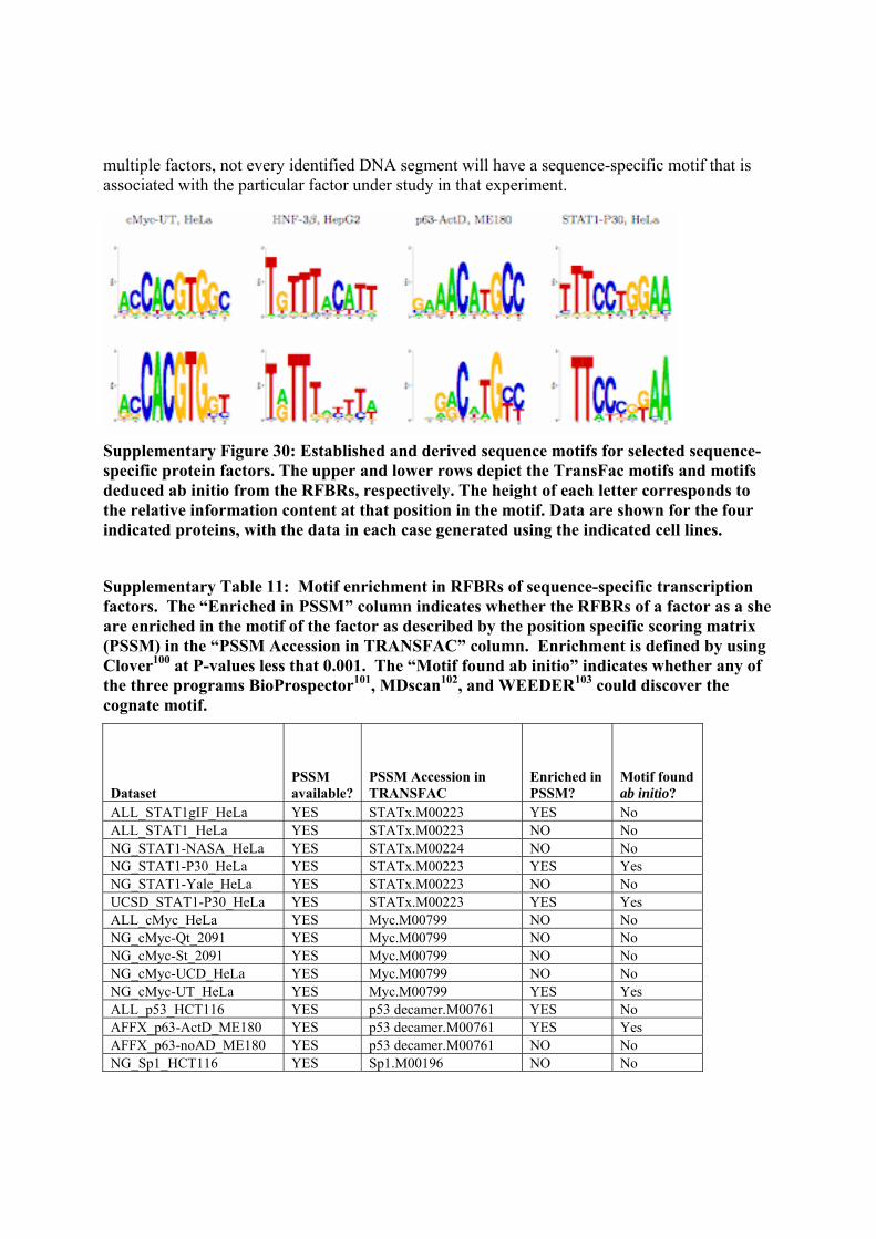
multiple factors, not every identified DNA segment will have a sequence-specific motif that is associated with the particular factor under study in that experiment.

Supplementary Figure 30: Established and derived sequence motifs for selected sequence-specific protein factors. The upper and lower rows depict the TransFac motifs and motifs deduced ab initio from the RFBRs, respectively. The height of each letter corresponds to the relative information content at that position in the motif. Data are shown for the four indicated proteins, with the data in each case generated using the indicated cell lines.

Supplementary Table 11: Motif enrichment in RFBRs of sequence-specific transcription factors. The “Enriched in PSSM” column indicates whether the RFBRs of a factor as a she are enriched in the motif of the factor as described by the position specific scoring matrix (PSSM) in the “PSSM Accession in TRANSFAC” column. Enrichment is defined by using Clover100 at P-values less that 0.001. The “Motif found ab initio” indicates whether any of the three programs BioProspector101, MDscan102, and WEEDER103 could discover the cognate motif.

Dataset PSSM available?

PSSM Accession in TRANSFAC

Enriched in PSSM?

Motif found ab initio?

ALL_STAT1gIF_HeLa YES STATx.M00223 YES No ALL_STAT1_HeLa YES STATx.M00223 NO No NG_STAT1-NASA_HeLa YES STATx.M00224 NO No NG_STAT1-P30_HeLa YES STATx.M00223 YES Yes NG_STAT1-Yale_HeLa YES STATx.M00223 NO No UCSD_STAT1-P30_HeLa YES STATx.M00223 YES Yes ALL_cMyc_HeLa YES Myc.M00799 NO No NG_cMyc-Qt_2091 YES Myc.M00799 NO No NG_cMyc-St_2091 YES Myc.M00799 NO No NG_cMyc-UCD_HeLa YES Myc.M00799 NO No NG_cMyc-UT_HeLa YES Myc.M00799 YES Yes ALL_p53_HCT116 YES p53 decamer.M00761 YES No AFFX_p63-ActD_ME180 YES p53 decamer.M00761 YES Yes AFFX_p63-noAD_ME180 YES p53 decamer.M00761 NO No NG_Sp1_HCT116 YES Sp1.M00196 NO No


NG_Sp1_JURKAT YES Sp1.M00196 NO No NG_Sp1_K562 YES Sp1.M00196 NO No NG_Sp3_HCT116 YES Sp3.M00665 NO No NG_Sp3_JURKAT YES Sp3.M00665 NO No NG_Sp3_K562 YES Sp3.M00665 NO No NG_E2F1_HeLa YES E2F.M00803 YES No NG_E2F4_2091 YES E2F-4:DP-1.M00738 NO No NG_cJun_HeLa YES CRE-BP1:c-Jun.M00041 NO No Sanger_HNF3b_HePG2 YES HNF-3.M00791 YES Yes Sanger_HNF4a_HePG2 YES HNF-4.M00134 YES Yes Sanger_USF1_HePG2 YES USF.M00217 YES No AFFX_CEBPe_HL60 YES C/EBP.M00770 YES Yes AFFX_CTCF_HL60 See Below N/A NO No AFFX_PU1_HL60 YES PU.1.M00658 NO No AFFX_RARecA_HL60 YES RAR.M00762 NO No AFFX_p300_HL60 YES p300.M00033 NO No NG_BAF155_HeLa NO N/A N/A N/A NG_BAF170_HeLa NO N/A N/A N/A UCSD_Suz12_HeLa NO N/A N/A N/A AFFX_Brg1_HL60 NO N/A N/A N/A AFFX_SIRT1_HL60 NO N/A N/A N/A FOS No RFBR at 5% FDR

S3.12 Significance of RFBR enrichments near GENCODE TSSs In order to assess the significance of enrichments of RFBRs near GENCODE TSSs, we have carried out a random simulation. First, we calculated the observed number of RFBRs near GENCODE TSSs for each ChIP experiment. Then, we randomly generated a set of fragments with their total number, length distribution, and ENCODE region distribution matching to those of the experimental RFBRs. This set was used to compute an expected number of RFBRs near TSSs. Repetitive elements were excluded in our simulation and the randomization was repeated 500 times to obtain the average expected number of RFBRs near TSSs. In the end, the observed number of RFBRs near GENCODE TSSs was divided by this expected number to yield the relative enrichment that is depicted on y-axis in Supplementary Figure 31. As shown in this figure, our simulation indicates that for most ChIP experiments the enrichment of their RFBRs near GENCODE TSSs is significant (>1.0). Each point in Supplementary Figure 31 represents one ChIP experiment.


Supplementary Figure 31: Distribution of RFBRs relative to GENCODE TSSs. The y-axis depicts the relative enrichment of RFBRs at GENCODE TSSs, while the x-axis shows the order of factors tested by ChIP experiments with respect to this enrichment. Random expectation corresponds to an enrichment of 1.0. Pink circles represent factors expected to be general for many promoters (e.g., polymerase), whereas blue circles represent factors expected to be more sequence-specific. A handful of representative factors are labelled.

S3.12.1 Supplemental table provided in accompanying Excel spreadsheet This table shows for each ChIP experiment the percentage of RFBRs in various distance (in a 1 kb increment) in relation to category A TSSs. Data in this table shows that more than half of RFBRs for SIRT1 are 20 kb away from TSSs and thus are generally in "gene deserts." This table is provided in the included supplemental Excel spreadsheet on the worksheet labeled S3.12.1.

S3.13 Integration approaches to generate Regulatory Cluster lists We implemented four complementary approaches to integrate the data from 129 ChIP datasets. The Z-score method (see Supplement S3.13.1 ) normalizes ChIP scores from individual experiments and assigns a cumulative normalised score to genomic intervals. The Naïve Bayes method (see Supplement S3.13.2 ) combines ChIP scores from different experiments after thresholding and weighting them based on a set of known promoters. Though both these methods use continuous ChIP scores, Naïve Bayes makes an assumption on how a typical promoter is


while Z-score treats all the datasets the same way. The third and fourth methods, tree-weighting (see Supplement S3.13.3 ) and majority-voting (see Supplement S3.13.4 ) use FDR thresholded ChIP scores. Tree-weighting method weights the counts from ChIP hits based on both the TSS enrichments of individual experiments and the correlation between experiments. The last method, majority-voting, evaluates the level of experimental support for each genomic position by taking into account the number of cross-lab, cross-platform or cross-factor ChIP hits matching that position. Each of these integration methods is described in detail below. From these four methods we constructed two composite lists: A "small union list" of 965 regions from the union of approaches 1 and 2 (Z-score and Naive Bayes) and a "large union list" of 1393 regions from the union of the four methods. Both of these lists are available from the UCSC browser.

S3.13.1 Integration Approach 1: Z-score method We first selected a set of promoter-specific experiments that we wished to integrate to identify potentially novel promoters30. We then matched corresponding datapoints between datasets. To accomplish this, we divided the ENCODE region into ~24,000 reference intervals that largely corresponded to the probes from the 2 PCR tiling arrays. The ChIP intensities were converted to Z-scores and assigned to the reference intervals. To identify genomic regions identified by multiple experiments, we then summed the Z-scores for each interval across all the experiments (setting negative Z-scores to zero). To estimate a P-value for the summed score of each interval, we shuffled the data for each experiment within the ~24,000 reference intervals and then re-summed the values. We repeated this 10 times, to get a confidence value for each of the ~24,000 intervals. We used a cutoff of p<0.001 to define a list of putative promoters from this integrated analysis and merged regions that were within 100 bp of each other.

Supplementary Table 12: Experimental data in the “promoter” group used in the Z-score based method.

Experimental data in "promoter" group for the Z-score method:

HCT116_Sp1_ChIP H4ac_K562_1.wig.txt

HCT116_Sp3_ChIP GM06990_61105_Regulome_ENCODE.txt

Jurkat_Sp1_ChIP K562_061105_Regulome_ENCODE.txt

Jurkat_Sp3_ChIP SKNSH_061105_Regulome_ENCODE.txt

K562_Sp1_ChIP CACO2_061105_Regulome_ENCODE.txt

K562_Sp3_ChIP encodeUcsdChipAch3Imr90_f.txt

CTCF_00hr encodeUcsdChipHeLaH3H4acH3_p0.txt

Brg1_00hr encodeUcsdChipHeLaH3H4acH4_p0.txt

CEBPe_00hr encodeUcsdChipHeLaH3H4dmH3K4_p0.txt

HisH4_00hr encodeUcsdChipHeLaH3H4RNAP_p0.txt


P300_00hr encodeUcsdChipHeLaH3H4stat1_p0.txt

Pol2_00hr encodeUcsdChipHeLaH3H4TAF250_p0.txt

PU1_00hr encodeUcsdChipHeLaH3H4tmH3K4_p0.txt

RARecA_00hr encodeUcsdChipMeh3k4Imr90_f.txt

H3K27T_00hr encodeUcsdChipRnapHct116_f.txt

SIRT1_00hr encodeUcsdChipRnapHela_f.txt

H3K4me1_GM06990_1.wig.txt encodeUcsdChipRnapImr90_f.txt

H3ac_GM06990_1.wig.txt encodeUcsdChipRnapThp1_f.txt

H3ac_K562_1.wig.txt encodeUcsdChipTaf250Hct116_f.txt

H3K4me2_GM06990_1.wig.txt encodeUcsdChipTaf250Hela_f.txt

H3K4me2_K562_1.wig.txt encodeUcsdChipTaf250Imr90_f.txt

H3K4me3_GM06990_2.wig.txt encodeUcsdChipTaf250Thp1_f.txt

H3K4me3_K562_1.wig.txt encodeUcsdNgHeLaH3K4me3_p0.txt

H4ac_GM06990_1.wig.txt encodeUcsdNgHeLaRnap_p0.txt

S3.13.2 Integration Approach 2: Naïve Bayes Method Training Set: We trained a Naïve Bayes classifier to predict regulatory regions. A training set of real TSS and non-TSS regions was built as follows. The set of real TSS (positive set) was based on CAGE (5' Cap Analysis of Gene Expression) and GIS-PET (Gene Identification Signature Paired-End ditag) clusters. All the CAGE tags in ENCODE regions were clustered and only clusters with 4 or more tags were kept, producing 797 examples. These 797 examples were further filtered by intersecting them with the 5'-ends of GIS-PETs in either HCT116 or MCF7 cell lines to obtain 223 positive examples. The negative regions were selected from deep introns (3rd or deeper) and the CDS parts of deep exons. The introns were verified not to overlap with exons from other transcripts, TARs or transfrags. These selection criteria resulted in 225 regions, spanning approximately 450kb. All possible uniformly distributed and non-overlapping windows of 300bp were extracted, which gave 1365 negative examples (negative set). Training of the Bayesian Model: For each region in the training set, the average ChIP enrichment scores corresponding to different ChIP experiments within a 1KB window around the TSS were extracted. Using these scores, each ChIP dataset was binarized at a cutoff that maximized the correlation between the training set and the binarized ChIP dataset. The training set thus consisted of positive and negative examples of a TSS, each associated with a binary vector describing the presence or absence pattern of each TF within that example region. The prediction of the model is the log odds of a TSS given data. The log odds of a TSS is defined as:

])|(

)|(log[dataallTSSnonP

dataallTSSPoddsogl TSS −=

Under the Naïve-Bayes assumption that all datasets are independent, the log odds can be separated into two terms:

∑ −==

+−

=dataall i

iTSS TSSnonxDP

TSSxDPTSSnonP

TSSPoddsogl ])|(

)|(log[])(

)(log[


The first term is the prevalence of the TSSs. In the second term, Di is a binary variable that denotes the ith dataset. If x=1 (i.e., the average score for ChIP dataset Di around the given TSS is above its threshold and hence the represented factor is present in the example), we call the contribution to the second term PLL (positive log likelihood) and if x=0 we call it NLL (negative log likelihood). For each dataset, both PLL and NLL were measured empirically from the training set. Scanning of ENCODE Regions with the Bayesian Model: Once the appropriate Bayesian weights were calculated (PLL and NLL), ENCODE regions were scanned using the model to predict new regulatory regions. To build a map of regulatory regions we calculated, for each base pair in the ENCODE regions, the log odds score of it being part of a TSS by summing contributions from individual ChIP datasets at that base pair. For each dataset, the contribution is either PLL or NLL depending on whether that base pair is called present or absent in that dataset based on the respective binarization cutoff. Contiguous base pairs with a log odds score above a chosen cutoff were joined to define putative regulatory regions. The final list of regions was obtained by pruning all the regions shorter than 300bp and by joining regions separated by less than 200bp. The score cutoff was calculated based on the expected prevalence of TSSs in the entire ENCODE region but was later made more stringent to obtain a higher confidence set of predictions.

S3.13.3 Integration Approach 3: Tree-weighting Method In this method, we first calculated the fold-enrichment Fi of RFBRs near TSSs for each experiment i. Briefly, the fold-enrichment was defined as the number of RFBRs near a TSS (-2 kb to +200 bp) divided by a corresponding number derived from a simulation in which the RFBRs for experiment i were randomly shuffled and placed back on the individual ENCODE regions (excluding repeats). Separately, we constructed a cluster tree of all ChIP experiments based on their similarities with regard to the genomic distribution of RFBRs. This is very similar to the construction of the whole-track correlation scores (described above). A weight Wi was assigned to each leaf (i.e., experiment i) using a branch-length division method104. The primary purpose of this clustering and weight-assigning step was to minimize the bias introduced by the same factors being tested in multiple conditions and several platforms. In this analysis, the overall weight for a particular factor would be apportioned between individual experiments with a ratio between 1/n and 1, where n is the number of experiments in which this factor was probed. We then made a union list of RFBRs from individual experiments on the condition that overlapping (by ≥ 50 bp) RFBRs were merged into a single region. This union contained 3227 regions (average length ~1.1 kb). A score Sj was subsequently assigned to each region j in the union list. It was defined as ∑ (Ni x Fi x Wi) where Ni was the number of RFBRs within this region j from experiment i, and Fi and Wi were the fold-enrichment and weight computed for experiment i, respectively. Finally, in order to make this integrative list comparable with those from the other three methods we used a Sj threshold of 0.05 to generate a total of 714 regions, based on the distribution of scores in these regions. This cutoff approximately corresponded to 2 ChIP hits per region.


S3.13.4 Integration Approach 4: Voting Method We developed a voting method to identify genomic regions that were determined by at least two ChIP datasets from different labs, or on different factors, or on different platforms. Each experiment was given a weight based on two measures: 1) the number of different investigators within ENCODE who studied the sequence-specific transcription factor, histone modification, PolII, or TAF1, 2) the number of different platforms used in these studies. An experiment would be assigned a maximum weight of one if the factor, modification, or binding in question was studied by a single investigator using a single platform type. Otherwise, a weight smaller than one and inversely proportional to the multiplicity was assigned. Supplementary Table 13 shows the weights used for each experiment. We used the weighted RFBRs to determine genomic regions marked by different groups of RFBRs at different FDR levels. The 129 experiments were stratified into two groups: those for sequence specific transcription factors (Sequence Specific Voting List) and the remaining ones for histone modifications, Pol2, and TAF1 binding. For each experiment, all the base pairs within an RFBR were assigned the same weight and for each base pair these weights were summed across all the experiments in each of the two groups. This gave a continuous score over the ENCODE regions. The score at a given base position is i) zero if that base doesn't appear in any of the RFBRs, ii) above zero if that base gets support from at least one experiment, iii) above one if that base is supported by at least two experiments done either using the same platform by different investigators or using different platforms by the same investigator. For each group, two different thresholds were used (zero and one) to convert the continuous scores to genomic regions. All the base pairs above the threshold were clustered together to define a genomic region whose score was the mean score for all the base pairs contained within it.

Supplementary Table 13: Weights used in the voting method.

Peakfile designfile InverseWeight Weight lab TR

HisPolTAF TF

AFFX_Brg1-00_HL60 Affy.all 8 0.125 Affy 1 0 1AFFX_Brg1-02_HL60 Affy.all 8 0.125 Affy 1 0 1AFFX_Brg1-08_HL60 Affy.all 8 0.125 Affy 1 0 1AFFX_Brg1-32_HL60 Affy.all 8 0.125 Affy 1 0 1AFFX_CEBPe-00_HL60 Affy.all 8 0.125 Affy 1 0 1AFFX_CEBPe-02_HL60 Affy.all 8 0.125 Affy 1 0 1AFFX_CEBPe-08_HL60 Affy.all 8 0.125 Affy 1 0 1AFFX_CEBPe-32_HL60 Affy.all 8 0.125 Affy 1 0 1AFFX_CTCF-00_HL60 Affy.all 8 0.125 Affy 1 0 1AFFX_CTCF-02_HL60 Affy.all 8 0.125 Affy 1 0 1AFFX_CTCF-08_HL60 Affy.all 8 0.125 Affy 1 0 1AFFX_CTCF-32_HL60 Affy.all 8 0.125 Affy 1 0 1AFFX_H3ac-00_HL60 Affy.all 8 0.125 Affy 1 1 0AFFX_H3ac-02_HL60 Affy.all 8 0.125 Affy 1 1 0AFFX_H3ac-08_HL60 Affy.all 8 0.125 Affy 1 1 0AFFX_H3ac-32_HL60 Affy.all 8 0.125 Affy 1 1 0AFFX_H4ac-00_HL60 Affy.all 8 0.125 Affy 1 1 0AFFX_H4ac-02_HL60 Affy.all 8 0.125 Affy 1 1 0


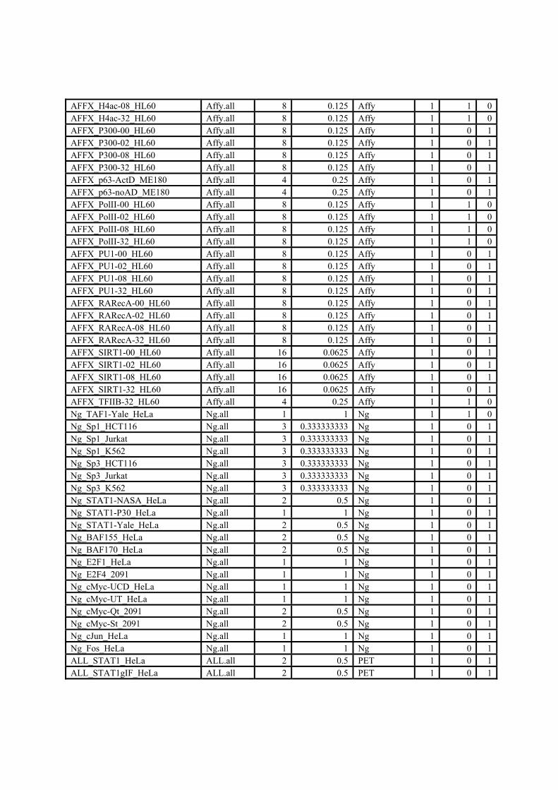
AFFX_H4ac-08_HL60 Affy.all 8 0.125 Affy 1 1 0AFFX_H4ac-32_HL60 Affy.all 8 0.125 Affy 1 1 0AFFX_P300-00_HL60 Affy.all 8 0.125 Affy 1 0 1AFFX_P300-02_HL60 Affy.all 8 0.125 Affy 1 0 1AFFX_P300-08_HL60 Affy.all 8 0.125 Affy 1 0 1AFFX_P300-32_HL60 Affy.all 8 0.125 Affy 1 0 1AFFX_p63-ActD_ME180 Affy.all 4 0.25 Affy 1 0 1AFFX_p63-noAD_ME180 Affy.all 4 0.25 Affy 1 0 1AFFX_PolII-00_HL60 Affy.all 8 0.125 Affy 1 1 0AFFX_PolII-02_HL60 Affy.all 8 0.125 Affy 1 1 0AFFX_PolII-08_HL60 Affy.all 8 0.125 Affy 1 1 0AFFX_PolII-32_HL60 Affy.all 8 0.125 Affy 1 1 0AFFX_PU1-00_HL60 Affy.all 8 0.125 Affy 1 0 1AFFX_PU1-02_HL60 Affy.all 8 0.125 Affy 1 0 1AFFX_PU1-08_HL60 Affy.all 8 0.125 Affy 1 0 1AFFX_PU1-32_HL60 Affy.all 8 0.125 Affy 1 0 1AFFX_RARecA-00_HL60 Affy.all 8 0.125 Affy 1 0 1AFFX_RARecA-02_HL60 Affy.all 8 0.125 Affy 1 0 1AFFX_RARecA-08_HL60 Affy.all 8 0.125 Affy 1 0 1AFFX_RARecA-32_HL60 Affy.all 8 0.125 Affy 1 0 1AFFX_SIRT1-00_HL60 Affy.all 16 0.0625 Affy 1 0 1AFFX_SIRT1-02_HL60 Affy.all 16 0.0625 Affy 1 0 1AFFX_SIRT1-08_HL60 Affy.all 16 0.0625 Affy 1 0 1AFFX_SIRT1-32_HL60 Affy.all 16 0.0625 Affy 1 0 1AFFX_TFIIB-32_HL60 Affy.all 4 0.25 Affy 1 1 0Ng_TAF1-Yale_HeLa Ng.all 1 1 Ng 1 1 0Ng_Sp1_HCT116 Ng.all 3 0.333333333 Ng 1 0 1Ng_Sp1_Jurkat Ng.all 3 0.333333333 Ng 1 0 1Ng_Sp1_K562 Ng.all 3 0.333333333 Ng 1 0 1Ng_Sp3_HCT116 Ng.all 3 0.333333333 Ng 1 0 1Ng_Sp3_Jurkat Ng.all 3 0.333333333 Ng 1 0 1Ng_Sp3_K562 Ng.all 3 0.333333333 Ng 1 0 1Ng_STAT1-NASA_HeLa Ng.all 2 0.5 Ng 1 0 1Ng_STAT1-P30_HeLa Ng.all 1 1 Ng 1 0 1Ng_STAT1-Yale_HeLa Ng.all 2 0.5 Ng 1 0 1Ng_BAF155_HeLa Ng.all 2 0.5 Ng 1 0 1Ng_BAF170_HeLa Ng.all 2 0.5 Ng 1 0 1Ng_E2F1_HeLa Ng.all 1 1 Ng 1 0 1Ng_E2F4_2091 Ng.all 1 1 Ng 1 0 1Ng_cMyc-UCD_HeLa Ng.all 1 1 Ng 1 0 1Ng_cMyc-UT_HeLa Ng.all 1 1 Ng 1 0 1Ng_cMyc-Qt_2091 Ng.all 2 0.5 Ng 1 0 1Ng_cMyc-St_2091 Ng.all 2 0.5 Ng 1 0 1Ng_cJun_HeLa Ng.all 1 1 Ng 1 0 1Ng_Fos_HeLa Ng.all 1 1 Ng 1 0 1ALL_STAT1_HeLa ALL.all 2 0.5 PET 1 0 1ALL_STAT1gIF_HeLa ALL.all 2 0.5 PET 1 0 1


ALL_cMyc_HeLa ALL.all 1 1 PET 1 0 1ALL_p53_HCT116 ALL.all 1 1 PET 1 0 1Sanger_H3ac_GM06990 Sanger.all 3 0.333333333 Sanger.PCR 1 1 0Sanger_H3ac_HeLa Sanger.all 3 0.333333333 Sanger.PCR 1 1 0Sanger_H3ac_K562 Sanger.all 3 0.333333333 Sanger.PCR 1 1 0Sanger_H4ac_GM06990 Sanger.all 3 0.333333333 Sanger.PCR 1 1 0Sanger_H4ac_HeLa Sanger.all 3 0.333333333 Sanger.PCR 1 1 0Sanger_H4ac_K562 Sanger.all 3 0.333333333 Sanger.PCR 1 1 0Sanger_H3K4me1_GM06990 Sanger.all 2 0.5 Sanger.PCR 1 1 0SUZ Sanger.all 2 0.5 Sanger.PCR 1 1 0Sanger_H3K4me2_GM06990 Sanger.all 3 0.333333333 Sanger.PCR 1 1 0Sanger_H3K4me2_HeLa Sanger.all 3 0.333333333 Sanger.PCR 1 1 0Sanger_H3K4me2_K562 Sanger.all 3 0.333333333 Sanger.PCR 1 1 0Sanger_H3K4me3-2_GM06990 Sanger.all 3 0.333333333 Sanger.PCR 1 1 0Sanger_H3K4me3_HeLa Sanger.all 3 0.333333333 Sanger.PCR 1 1 0Sanger_H3K4me3_K562 Sanger.all 3 0.333333333 Sanger.PCR 1 1 0Ng_H3ac-P0_HeLa Ng.all 2 0.5 UCSD.Ng 1 1 0Ng_H3ac-P30_HeLa Ng.all 2 0.5 UCSD.Ng 1 1 0Ng_H4ac-P0_HeLa Ng.all 1 1 UCSD.Ng 1 1 0Ng_H3K4me2-P0_HeLa Ng.all 2 0.5 UCSD.Ng 1 1 0Ng_H3K4me2-P30_HeLa Ng.all 2 0.5 UCSD.Ng 1 1 0Ng_H3K4me3-P0_HeLa Ng.all 2 0.5 UCSD.Ng 1 1 0Ng_H3K4me3-P30_HeLa Ng.all 2 0.5 UCSD.Ng 1 1 0Ng_PolII-P0_HeLa Ng.all 2 0.5 UCSD.Ng 1 1 0Ng_PolII-P30_HeLa Ng.all 2 0.5 UCSD.Ng 1 1 0UCSD_H3ac_IMR90 UCSD.all 2 0.5 UCSD.PCR 1 1 0UCSD_H3ac-P0_HeLa UCSD.all 4 0.25 UCSD.PCR 1 1 0UCSD_H3ac-P30_HeLa UCSD.all 4 0.25 UCSD.PCR 1 1 0UCSD_H4ac-P0_HeLa UCSD.all 2 0.5 UCSD.PCR 1 1 0UCSD_H4ac-P30_HeLa UCSD.all 2 0.5 UCSD.PCR 1 1 0UCSD_H3K4me2_IMR90 UCSD.all 2 0.5 UCSD.PCR 1 1 0UCSD_H3K4me2-P0_HeLa UCSD.all 4 0.25 UCSD.PCR 1 1 0UCSD_H3K4me2-P30_HeLa UCSD.all 4 0.25 UCSD.PCR 1 1 0UCSD_H3K4me3-P0_HeLa UCSD.all 2 0.5 UCSD.PCR 1 1 0UCSD_H3K4me3-P30_HeLa UCSD.all 2 0.5 UCSD.PCR 1 1 0UCSD_PolII-P0_HeLa UCSD.all 8 0.125 UCSD.PCR 1 1 0UCSD_PolII-P30_HeLa UCSD.all 8 0.125 UCSD.PCR 1 1 0UCSD_PolII_HCT116 UCSD.all 4 0.25 UCSD.PCR 1 1 0UCSD_PolII_IMR90 UCSD.all 4 0.25 UCSD.PCR 1 1 0UCSD_PolII_THP1 UCSD.all 4 0.25 UCSD.PCR 1 1 0UCSD_TAF1_HCT116 UCSD.all 4 0.25 UCSD.PCR 1 1 0UCSD_TAF1_IMR90 UCSD.all 4 0.25 UCSD.PCR 1 1 0UCSD_TAF1_THP1 UCSD.all 4 0.25 UCSD.PCR 1 1 0UCSD_TAF1-P0_HeLa UCSD.all 8 0.125 UCSD.PCR 1 1 0UCSD_TAF1-P30_HeLa UCSD.all 8 0.125 UCSD.PCR 1 1 0UCSD_STAT1-P30_HeLa UCSD.all 2 0.5 UCSD.PCR 1 0 1Sanger_HNF3b_HePG2 Sanger.all 1 1 Sanger.PCR 1 0 1


Sanger_HNF4a_HePG2 Sanger.all 1 1 Sanger.PCR 1 0 1Sanger_USF1_HePG2 Sanger.all 1 1 Sanger.PCR 1 0 1

S3.13.5 Site detection algorithm The site detection algorithm employs a rank statistics based paradigm where all enrichment sites are ranked based on their intra-replicate ranks and inter-replicate rank consistency. The two fundamental parameters of the site detection model are: (a) signal enrichment; (b) pScore where

( )( )pValuepScore p 10log10−== σ . The first step in the algorithm entails the application of a lenient threshold, approximating a signal to noise ratio (SNR) slightly greater than 1. This estimate, based on either a fixed pScore (20) or a signal enrichment (log(2)) threshold, captures the maximal number of candidate intervals or seed sites. The second step refines the seeding process and associates statistical significance to each site. This optimization is governed by the following parameters determined both on an intra and inter array basis. Specifically on a per site basis, they comprise of: (a) Rank of pScore per replicate; (b) Sum of the absolute pair-wise rank difference (SAD) across replicates; (c) χ2 based composite P-value estimate across replicates; The basic optimization in the model involves: minimization of the above three parameters with simultaneous maximization of signal enrichment. Ultimately, seed sites with superior intra-replicate ranks as well as high rank consistency across replicates are expected to dominate the highly significant set of the final sites. The site rankings are accompanied by site-level meta P-value and composite signal enrichment across replicates. Further segmentation of the ranked sites is possible via P-value or signal enrichment criteria individually or by a criterion derived from the composite. Sensitivity (reported for H4ac data) obtained following segmentation of data using the filters: (a) meta P-value of 10-5: 88%; (b) array enrichment of 0.2: 87%; (c) composite of (a) and (b): 95%.


Supplementary Figure 32: Comparison of the composite Regulatory Cluster lists generated by four methods. The four methods independently generated 793 (NB), 656 (Z), 828 (TW), and 1327 (V) Regulator Clusters respectively. To make the data directly comparable and resolve the caveat that a region from one method could overlap with multiple regions in another method, we had collapsed all regions from these four methods into 1393 non-overlapping regions. This process resulted in 689, 580, 714, and 985 regions respectively for the four methods above. Shown in this Venn diagram is the partition of these 1393 regions into different sets according to how many methods identified them. For instance, 340 regions were identified by all four methods. Numbers not shown include 6 between NB and TW only and 19 between V and Z only. All numbers sum up to 1393 non-overlapping regions.

S3.14 The overlap of Regulatory Clusters with different TSS evidence classes. The correspondence of the regulatory clusters with the previously categorized TSSs was investigated by examining the numbers of clusters falling within 2.5kb of TSSs from each category. The table below shows the number and percent of 1393 Regulatory Clusters located within 2.5kb of a Transcription Start Site (TSS) from one of categories. TSS Categories as defined in Table 3 of the main paper. Because a given Regulatory Cluster can fall within 2.5kb of more than one TSS the total of the percents exceeds 100.


Supplementary Table 14: Overlap of Regulatory Clusters with different TSS evidence classes.

TSS Category (number of TSS in category)

NUMBER OF REGULATORY

CLUSTERS

PERCENT OF REGULATORY

CLUSTERS GENCODE 5’ ends (1730) 595 42.7 Novel: Sense exon (1437) 405 29.1 Novel: Antisense exon (521) 283 20.3 Novel: TxFrag/RxFrag (639) 363 26.1 Novel: CpG (164) 128 9.2 As Supplementary Table 14 shows, there is a bias towards the GENCODE 5’ ends, but not obviously across the other classes.

S3.15 Cloning putative novel promoters Of the 233 putative promoters that were cloned and tested, 186 had at least one CAGE or GIS-PET supporting a TSS in that region (of these 186, 113 had only one tag). The remaining 47 putative promoter fragments had no transcript data that supported a TSS in that region. For the 186 that had CAGE or GIS-PET support, we used the 5’ end of the CAGE or GIS-PET sequence as the predicted TSS. We then used Primer3 software to design primers by inputting 600 bp of upstream sequence and 100bp downstream of the predicted TSS105. Each primer pair was required to flank the transcription start site. For the 47 promoters that lacked transcripts we designed primers to amplify a 1000 bp fragment so that we could clone it in both directions. To the 5’ end of each primer, we added 16 basepair tails to facilitate cloning by the Infusion Cloning System (BD Biosciences, Clontech cat no. 639605). (Left primer tail: 5’-CCGAGCTCTTACGCGT-3’, Right primer tail: 5’-CTTAGATCGCAGATCT-3’) We amplified the fragments using the touchdown PCR protocol previously described106 and Titanium Taq Enzyme (BD Biosciences, Clontech, cat no 639210). To clone our PCR amplified fragments using the Infusion Cloning System, we combined 2 μl purified PCR product and 100 ng linearized pGL3-Basic vector (Promega). We added this mixture to the Infusion reagent and incubated at 42°C for 30 minutes. After incubation, the mixture was diluted and transformed into competent cells (Clontech cat. No. 636758). We screened clones for insert by PCR and positive clones were prepared as previously described. We quantified DNA with a 96-well spectrophotometer (Molecular Devices, Spectramax 190) and standardized concentrations to 50 ng/μl for transfections.


Supplementary Table 15: Overlap of Experimentally Tested Regulatory Clusters with TSS Categories. The table lists experimental validation results for all the regulatory clusters that were tested by transient-transfection reporter assay (TFXN) and/or RACE. A regulatory cluster might overlap with more than one type of TSS category

TSS Categories

A B C D E F no_ABC

DE no_ABCDEF Pos 3 1 0 1 0 1 1 1 0 Neg 17 3 4 7 8 2 3 4 3 Both

Tested (Pos+Neg) 20 4 4 8 8 3 4 5 3 Pos 85 24 19 14 28 9 23 29 21 Neg 120 13 13 10 20 9 30 78 59 Either

Tested (Pos+Neg) 205 37 32 24 48 18 53 107 80 Pos 41 8 9 4 12 5 14 16 10 Neg 122 13 12 12 25 10 31 76 57 TFXN

Tested (Pos+Neg) 163 21 21 16 37 15 45 92 67 Pos 47 17 10 11 16 5 10 14 11 Neg 15 3 5 5 3 1 2 6 5 RACE

Tested (Pos+Neg) 62 20 15 16 19 6 12 20 16

Supplementary Figure 33: Example of a novel promoter supported by the reporter assay and RACE products. a) Region predicted to contain a novel promoter based on the integrated analysis b) Activity of the novel predicted promoter as assayed by the transient


transfection reporter assay c) 5’ RACE products show the 5’ end of a novel transcript occurs in the novel promoter region d) Annotated RefSeq genes e) Annotated human mRNAs f) Computationally predicted CpG islands g) Transcribed regions experimentally identified with genomic tiling microarrays h) Maps of experimentally identified transcription start sites based on CAGE and GIS-PET sequences i) Fragments assayed for promoter activity by transiently transfected reported constructs (intensity of red is proportional to promoter activity) j) Binding sites of various transcription factors identified by chromatin IP and tiling microarrays. This figure was adapted from the UCSC genome browser.

S3.15.1 Cell culture, transient transfections, and reporter gene activity assays We performed transfections in 4 cultured human cell lines (Hela, HCT116, HT1080, and CRL1690) as previously described106. We seeded 5,000-10,000 cells per well in 96-well plates. Twenty-four hours after seeding, we co-transfected 50 ng of each experimental luciferase plasmid with 10 ng of renilla control plasmid (pRL-TK, Promega Cat. No. E2241) in duplicate using 0.3 μl of FuGene (Roche) transfection reagent per well. We also transfected 24 random genomic fragments as negative controls. Cells were lysed 24-48 hours post-transfection, depending on cell type. We measured luciferase and renilla activity using the PE Wallac Luminometer and the Dual Luciferase Kit (Promega, Cat. No. E1960). We followed the protocol suggested by the manufacturer with the exceptions of injecting 60 μl each of the luciferase and renilla substrate reagents and reading for 5 seconds.

S3.15.2 Data Analysis The activity data is reported as a transformed ratio of luciferase to renilla. The mean ratio and standard deviation in the 4 cell lines were computed for 24 negative controls. The final promoter activity was computed as the number of standard deviations from the mean for each promoter in each cell line. All the promoters which were at least three standard deviations above the mean ratio of the negatives were called significantly positive.

S3.16 Control for the Ascertainment Bias The raw enrichment signal of 23 ChIP-chip datasets were compiled for 28 non-GENCODE based clusters. The signals from multiple ChIP-chip regions matching the same regulatory cluster were averaged. For each ChIP-chip dataset, a Mann-Whitney test was performed to compare the signal for 22 RACE-positive and 6 RACE-negative clusters. Supplementary Table 16 lists the two-tailed p-values. None of the datasets suggests that there is a difference in the raw signal for positives vs. negatives.

Supplementary Table 16: Significance from rank sum test for 22 Novel RACE Positive and 6 Novel RACE Negative regulatory clusters.

ChIP-chip Dataset pvalue


ChIP-chip Dataset pvalue

Stanford_Sp1_HCT116 0.112

Stanford_Sp1_Jurkat 0.892

Stanford_Sp1_K562 0.088

Stanford_Sp3_HCT116 0.395

Stanford_Sp3_Jurkat 0.427

Stanford_Sp3_K562 0.157

UCDavis_E2F1_HeLa 0.723

UCDavis_Myc_HeLa 0.978

UCSDNg_H3ac_HeLa_p0 0.604

UCSDNg_H3ac_HeLa_p30 1

UCSDNg_H3K4me2_HeLa_p0 0.892




UCSDNg_H4ac_HeLa_p0 0.643

UCSDNg_Pol2_HeLa_p0 0.530

UCSDNg_Pol2_HeLa_p30 0.806

UCSDNg_STAT1_HeLa_p30 0.039

UCSD_STAT1_HeLa_p0 0.764

UCSD_STAT1_HeLa_p30 0.604

UCSD_Suz12_HeLa 0.654

UT_cMyc_HeLa 0.460

UT_E2F4_2091Fibroblast 0.643

S3.17 Classification of functional elements

S3.17.1 SVM Classification of functional elements We used the Support Vector Machine algorithm to classify DHS segments on the basis of histone modification data. We designed classifiers to distinguish the signature or histone modifications patterns in distal and proximal distance with respect to GENCODE transcriptional start sites.

S3.17.1.1 SVM discrimination of proximal DHS vs. non-proximal DHS (1) We begin by determining the distance between each DHS and the nearest GENCODE Gene. The GENCODE gene used in the analysis are an aggregate of the known, pseudo, and putative GENCODE subtracks. (2) Once the distance is calculated, each DHS is placed into a proximal or non-proximal category. In order to be considered proximal, a DHS must be within +/- 2500 bases of a GENCODE Tx start. We place all other DHSs in the nonproximal category. Each DHS is now


assigned an SVM training 'label', representing whether or not it is proximal to a GENCODE Gene. (3) All DHS segments are then expanded in each direction until the total segment length is 1000bp. (4) We assign the mean score of each histone modification is assigned to each 1000bp expanded DHS. This produces a vector of 5 scores for each DHS. (5) All histone scores are translated to standard units (Zscores) by using the mean and standard deviation of all results from a given assay over the entire ENCODE regions. (6) If a DHS does not contain a full set of histone modification scores (due to gaps in the underlying assay), the entire DHS is eliminated from the analysis. (7) We prepare the SVM input by placing each labeled DHS, and the associated histone modification scores, into a matrix. (8) Training and cross-validation results are generated by running a grid of SVM simulations using the freely available SVM implementation, PyML toolkit (http://pyml.sourceforge.net). We choose the best SVM resulting from 10-fold cross-validation of the training set. Each round of cross validation consists of training the SVM on a randomly selected 90% of the data, and then measuring the results against the held out 10%. An individual iteration of cross-validation performs model selection to select the best combination of SVM parameters. The specific parameters evaluated during model selection are Gaussian kernel gamma values of 0.01,0.1,1,10, and kernel 'C' values of 0.1,1,10,100.

S3.17.1.2 SVM discrimination of proximal DHS from random background We perform step #1 as in section S3.17.1.1 (2) We assign positive labels to all DHSs within +/- 2500bp of a GENCODE Tx Start. These DHSs are considered proximal-DHSs. (3) Next, we begin collecting the negative SVM training examples. First, all ENCODE regions are broken into contiguous 250bp segments. Segments located within 2kb of a proximal-DHS are removed from the data set. (4) All segments are expanded to 1kb. (5) We assign the mean score from each histone assay to the corresponding 1kb segment. Any segments that do not have an associated score are removed from the data set. (6) Since the resulting negative data set is quite large, we randomly sample segments until we have satisfied a ratio of 2 negatives examples for every positive example. We then perform steps 7-10 as above.

S3.17.1.3 SVM discrimination of distal DHSs from background We perform step #1 as in section S3.17.1.1. We then assign positive labels to all DHSs that are more than 10kb from the nearest GENCODE Tx Start. These DHSs are considered distal-DHSs. We then perform steps 3-7 as in section S3.17.1.2

S3.17.1.4 ROC curves for individual histone marks (simple classifiers) The individual feature ROCs are determined by comparing the distribution of individual feature data to the training labels. The feature data is sorted in reverse order, and then the list of labels is traversed. Each time a label occurs out of order, the false positive count increases. If labels are in


consecutive order, the true positive count increases. The entire list is traversed in this manner. The resulting labels are plotted. The area under this curve is the feature-roc 'score'.

Supplementary Figure 34: Inputs to the two SVMs for discriminant training and their resulting performance. Panel A shows the classifier for distinguishing proximal from distal sites. Panel B shows the classifier for distinguishing TSSs from expressed vs non expressed transcripts. In each case, the upper portion summarizes the training data, while the lower portion consists of the Receiver Operating Characteristic (ROC) curves, in which the percent true-positive results (y-axis) are plotted as a function of the percent false-positive results (x-axis). A perfect classifier would have a step function that immediately achieves 100% true-positive results with no false predictions. A random classifier is a diagonal line between the bottom left and top right. The thick red line in each case shows the ROC curve of the SVM, whereas the different dashed lines show the curves for each individual mark independently.

S3.17.1.5 Correspondence of SVM identified TSSs with Gencode and Tag derived TSS categories.

The correspondence of the 110 top scoring TSSs identified by the SVM on the basis of Histone signals around DHSs to the category A-F TSSs in Table 3 (of the main paper) was investigated. The category A-F TSSs were characterised by a single genomic coordinate and the SVM-TSSs by an arbitrary 250bp region.


As the methodologies underlying the SVM-TSS identification have a poor resolution in base-pair coordinates we considered overlap to have occurred if features from the two classes fell within 2500bp of one another. Overlap analysis of the SVM-TSSs with the category A-F TSSs using the Genome Structure Correction (see section S1.3 ) for probability estimation is shown in Supplementary Table 17. The total number of SVM-TSSs located within 2500bp of a category A-F TSS was 93.

Supplementary Table 17: Counts of the numbers of SVM-TSSs falling within +/- 2500 bp of Category A-F TSSs and the probability of this occurring by chance – calculated using the GSC statistic. Note: the sum of the counts totals more than 110 as a given SVM-TSS can lie within 2500bp of more than one Category TSS.

TSS Category

Observed Overlay(count of SVM-TSSs)

p value

A 73 4.52E-018 B 51 3.05E-005 C 42 1.11E-016 D 32 9.87E-008 E 18 2.62E-043 F 38 1.26E-006

S3.17.2 CART Analysis of gene status CART as employed here is a classification algorithm – its background and theory are given in Classification and Regression Trees107. Like all such algorithms it constructs a rule for prediction of a particular label from a given set of variables. Again, like all such algorithms, CART needs to be provided with a training set, that is, a set of labeled examples from which to construct the rule. Once constructed, the rule’s performance is ideally judged on a test set for which the predictions of the classifier can be compared to known, true labels. CART is a tree structured algorithm. How it works is best illustrated when there are only two possible labels, for example, 0 and 1. Say we are given a categorical prediction variable with 10 possible categories and a real valued prediction variable. CART considers two types of rules based on one variable. For the categorical variable Y, the possible rules are an assignment of one of the two classes to each category. For instance, “If Y is category v, then assign label 0, else, assign label 1.” For the real variable X, the rules are of the form, “Assign label 0 if X < c and 1 if X > c, where c and the label identities are free. Each such rule can be framed as a question, such as above, with an answer: Yes, say, for a label 0, and No for a label 1. The program picks the “best” question (according to a purity measure described107 based on any one of the predictor variables, represents it as the root of the tree, and places the cases according to their answers. The resulting nodes are then subjected to the same procedure until all nodes


contain cases with the same label. The tree is then “pruned” back, since the pure tree, which, by construction, behaves optimally on the training sample, performs poorly on the test sample. Various methods of pruning are described in Breiman et al107. Performance on the test sample yields estimates of misclassification probabilities. Care has to be taken if the proportional sizes of the sets of examples corresponding to each label in the training set do not reflect their expected values in the population. Modifications to take care of such cases and the parallel situation that misclassification of one label is more serious than that of the others are available in the CART program. Tree structured rules have the advantage, which we try to employ, that, if the signal is strong, the order of the variables used in the “best” questions and their success in classification at the appropriate node give an indication of which variables may be important. Here, we have utilized CART to predict gene expression status based on several genomic and epigenomic variables, both categorical and real valued. We discovered that histone 3 lysine 4 methylation status (i.e. H3K4me1, H3K4me2, and H3K4me3), along with a measure of DNase sensitivity was sufficient to build high-quality predictors of gene expression status within, and to a lesser extent, between cell lines. Some of the input variables, such as CpG status (a 1,0 categorical variable indicating whether the transcription start site of the given gene occurs in a CpG island), appear to hold little to no predictive value in the presence of the other predictors, while others provide highly incisive questions, whose answers result in accurate labels for both training set and test set data.

S4 Chromatin architecture

S4.1 Replication Timing: Data generation and Analysis

S4.1.1 Determination of replication time of ENCODE regions HeLa cells were synchronized by a thymidine aphidicolin block and released from the block. As cells passed synchronously through a 10 hr S phase, they were labeled for 2 hr intervals with Bromodeoxyuridine starting at 0, 2, 4, 6 and 8 hrs. The BrdU labeled DNA was purified by two cycles of CsCl density gradient centrifugation, labeled and hybridized to the genome tiling arrays. Details of protocols and data processing are published in Jeon et al7 and Karnani et al8.

S4.2 Correlations between continuous chromatin and replication datatypes

S4.2.1 Sliding window correlations

S4.2.1.1 Background “Continuous” datatypes refer to those data that take on real values at nearly regularly-spaced intervals along the genome. Examples incude DNaseI sensitivity and DNA replication timing. This is in contrast to “discrete” datatypes that are elemental in nature, such as locations of DNaseI hypersensitive sites. The primary challenge for continuous analysis is the issue of scale. As inputs to the analysis, we are dealing with apparently disparate datatypes, collected at different resolutions and scales. Sanger histone modification strength data, for instance, is


available at a resolution of approximately 1kb, while PhastCons conservation scores are available at every base. We also have an issue of scale on the output side, in that we want to uncover trends in the data that may be occurring at multiple scales. The primary tool we use to address the challenge of scale is wavelets108, a mathematical tool pioneered in the field of signal processing. Wavelets provide a framework for decomposing a given data type into increasingly coarse scales, allowing broader and broader trends in the data to reveal themselves. As opposed to Fourier analysis, which also provides a decomposition of a given signal in terms of multiple scales (frequencies), wavelet analysis localizes behavior in both frequency and “time” (genomic position, in our case), and is thus better suited to pick up transient behavior. Wavelets have been used for the analysis of genomic data to uncover local periodic patterns in DNA bending profiles109 and gene expression data110, 111, to predict protein structures112, and to correlate a variety of genomic data on multiple scales in microbial genomes113. We use wavelets to visually represent individual datatypes on multiple scales at once, using wavelet scalograms, or heatmaps. Wavelets also provide a method to normalize pairs of datatypes to a common set of scales, allowing us to perform quantitative correlations on a scale-by-scale basis.

S4.2.1.2 Continuous wavelet transformation Wavelet analysis makes use of two types of transform, the continuous wavelet transform (CWT) and the discrete wavelet transform (DWT). The CWT is defined for a time series x(t) at each time t and scale a by

where ψ(t) is the wavelet function of choice. For this analysis we use the first derivative of Gaussian (DOG) wavelet, implemented in the R package Rwave. In this implementation the DOG wavelet is complex-valued, and the absolute value |W(a,t)| can be taken to represent the strength of the change in the original function x at scale a and location t. Thus for fixed a, |W(a,t)| can be thought of as a representation of x(t) at scale a. The Rwave wavelet functions are scaled so that the wavelet scale a is approximately equal to the equivalent Fourier period of a periodic feature in the original data, a fact we verified experimentally.

S4.2.1.3 Discrete wavelet transformation The discrete wavelet transform (DWT) is essentially defined by restricting the CWT to time series sampled at discrete, equally-spaced time points, and by restricting the scales to the dyadic intervals , where δ is the resolution of x. The DWT requires that the input sample x be of length equal to a power of two. A key feature of the DWT, not available for generic CWTs, is the multiresolution analysis. This gives, for each user-defined maximal level J corresponding to scale 2Jδ, a scale-by-scale decomposition of x into separate components,


Here the Dj, or details, represent the local change in x at the scale 2jδ, and the smooth SJ represents a smoothed version of x at the scale 2Jδ. The Dj and SJ are each the same length as x. For this analysis, we use a variant of the DWT called the maximal overlap DWT (MODWT), which allows x to be of arbitrary length. We use MODWT smooths for computing higher-order functional domains (see section S4.7 ) and for smoothing datasets in preparation for further analysis (see section S4.2.1.4 ). For all calculations we use the R package waveslim, and its implementation of the Daubechies “least asymmetric” LA(8) wavelet filter. We use reflection boundary conditions for computing multiresolution analyses.

S4.2.1.4 Preparation of ENCODE data sets for wavelet analysis Implementations of the CWT and MODWT require input datasets to be equally-spaced. We thus define a nominal scale for each ENCODE dataset based on the assay used in each case (50bp for DNaseI sensitivity, 1kb for Sanger histone modifications, for instance). We then construct equally-spaced datasets at the nominal scale using the following interpolation scheme. Gaps less than 2kb are filled using linear interpolation between the existing flanking data points. For gaps greater than 2kb, a linear loess curve is fit at each interpolated position, using data within a centered window of width equal to 50 times the gap length. We use R function loess with default weights. To compare datasets with disparate nominal scales, we transform the dataset with the finer nominal scale by computing its MODWT wavelet smooth (see section S4.2.1.3 ) at the dyadic scale closest to coarser scale.

S4.2.1.5 Wavelet correlations and correlation heatmaps Wavelet correlation heatmaps quantify the degree of local correlation between two genomic series on a scale-by-scale basis. For fixed scale a and genomic position t0 the wavelet coefficients at scale a for the two series are computed in a 20kb window centered at t0. The Pearson correlation coefficient is then computed on the two 20kb segments. The color in the correlation heatmap at location (t0,a) represents the correlation coefficient so computed, ranging from red (high) to yellow (none) to green (low). We use the DOG wavelet for computing wavelet correlations.

Supplementary Table 18: Significance of differences in sliding window correlation distributions. Wavelet sliding window correlation values between DNaseI and five activating histone modifications were computed as described above, and accumulated at the 16kb scale across all of ENCODE. The resulting distributions of correlation values were compared pairwise using the one-sided Kolmogorov-Smirnov test (R function ks.test). P-values, included below, were computed for the null hypothesis that the distribution for one mark (given by the row labels) is not greater than the distribution for the other mark (given by the column labels).

H3K4me2 H3K4me3 H3K4me1 H3ac H4ac H3K4me2 3.367152e-02 1.890608e-59 0.00982103 5.696281e-35 H3K4me3 0.008147442 1.391836e-63 0.01158146 1.667976e-36 H3K4me1 0.995825313 9.582033e-01 0.98030121 5.423018e-01


H3ac 0.001563221 2.519860e-06 1.118025e-55 1.465513e-33 H4ac 0.997792115 9.950358e-01 6.036933e-05 0.98488594

S4.2.1.6 Non-wavelet sliding window correlation for TR50 comparisons Correlations with DNA replication timing data, as represented by the TR50 curve, are handled separately. This is due to the highly smoothed nature of the TR50 data, which gives features that are of a scale beyond those used for the wavelet analyses of other datatypes. To reach the apparent scale of the TR50 data, we performed loess smoothing on the other datatypes. We experimented with a number of different window widths for loess smoothing -- a visual check revealed that a 100kb smoothing window produced features comparable to those of the TR50 data. Local correlations between TR50 and the loess smoothed datatypes are computed using a sliding window of 250kb, as in the previous section. This gives a vector of correlation values at a single scale (that of the loess smoothed data) as opposed to the multiple scales computed for other datatypes using wavelets.

S4.3 Correlations of histone modifications with TR50 at discrete points in the genome

In addition to the sliding window correlation analysis reported in Figure 7a, we computed a histogram of correlation values obtained for each histone modification vs. TR50 across all of ENCODE, and plotted these as a function of correlation value (Supplementary Figure 35). As expected, the activating marks were mostly negatively correlated with TR50, although there were occasional areas of positive correlation. H3K27me3 displays a greater heterogeneity of correlation , with the positive correlation slightly predominating. Indeed, experiments on random data indicate that the observed fraction of highly positive correlations of H3K27me3 (> 0.5) is statistically significant, with empirical p-value of 0.005 (see Supplement S4.3.1 ). The positive correlation is consistent with the enrichment of H3K27me3 in late replicating regions , and its depletion in early replicating regions, illustrated in Figure 7b. In mouse histone modification H3K27me3 is targeted to the promoters of genes that also exhibit high levels of H3K4 methylation in stem cells where repressed promoters are held poised for activation114. Intriguingly, this bivalent state disappeared in differentiated cells. A reappearance of the bivalent state in cancer cells could provide a potential explanation for the appearance of H3K27Me3 in early replicating regions in HeLa cells. An alternative explanation might be based on the interallelic variation in time of replication (pan-S replication) and interallelic variation in chromatin structure described in the text.

S4.3.1 Statistical significance of positive correlations between H3K27me3 and TR50

Sliding window correlations between TR50 and loess-smoothed H3K27me3 were computed as in section S4.2.1.6 and the resulting distribution of correlation values is displayed in Supplementary Figure 36. We observed that 28.3% of all ENCODE-wide sliding correlation values were greater than 0.5. To test the statistical significance of this result we performed sliding window correlation analysis on random data, simulated by randomly sampling the


H3K27me3 and TR50 datasets separately. Specifically, data for each of H3K27me3 and TR50 are concatenated across all of ENCODE to form two master datasets. Each sample experiment consisted of choosing, for each ENCODE region, a chunk of contiguous data of the same size as the given ENCODE region but starting from a random location in the H3K27me3 master dataset, and a separate same-sized chunk from a different random location in the TR50 master dataset. This was repeated for all 43 ENCODE regions (the TR50 data does not cover ENm011), and sliding window correlation was performed on the resulting 43 paired datasets. The sample experiment concluded by comparing the accumulated distribution of correlation values against the observed distribution. Out of 1000 such experiments, five produced distributions whose fraction of highly-positive correlations (>0.5) exceeded the observed fraction of 28.3%, for an empirical p-value of 0.005.

S4.3.2 Details of data analysis for Figure 7a Data for H3K4me2 and H3K27me3 are loess smoothed as described in section S4.2.1.6 and local correlations with TR50 are computed in a sliding 250kb window. The graphs are colored at each position to reflect the value of the local correlation at that point, with red representing positive correlation, green for negative correlation, and yellow for no correlation. Enrichment in Fig. 7a measures the strength of the signal for a particular mark at that location relative to the negative control ChiP. For H3K4me2 this is measured as the fold-enrichment while for H3K27me3 the measure is the negative log P value of the significance of enrichment.


Supplementary Figure 35: Smoothed histograms of all sliding window correlation values (of indicated histone modification enrichment versus TR50) computed as described in Section S4.3.2 and accumulated across all of ENCODE. The indicated histone modifications are largely anti-correlated with TR50. The vertical dashed lines indicate the mean correlation value for that mark. The smoothed histogram was computed and plotted using R function density(), using default optional arguments.


Documents

Identification and analysis of functional elements in -