Identification from Moment Conditions with

Singular Variance

Nicky Grant∗

Faculty of Economics

University of Cambridge

November 7, 2012

Abstract

This paper studies identification robust inference from moment conditions with

a singular variance matrix at the true parameter. An equivalence between singular

variance and identification failure is established for a wide class of moment functions.

The Generalized Anderson Rubin (AR) statistic is shown not to exist at the true

parameter with singular variance. A novel asymptotic approach is devised to provide

general asymptotic theory making no assumption on the rank of the moment variance

matrix. Conditions for which the AR statistic is asymptotically locally chi-squared

with singular variance are established. The 2-Step GMM (2S) statistic is shown to

have a non-standard distribution with singular variance. Tests of the rank of the

moment variance matrix and methods to correct the size of the confidence regions

based on the 2S statistic are provided. An extensive simulation study verifies the key

results of this paper.

Keywords: GMM, Anderson Rubin Statistic, Singular Variance, Identification.

JEL Classification: C10, C13, C58

∗Author Correspondence: Robinson College, Grange Road, Cambridge, CB3 9AN. nlg24@cam.ac.uk

1

1 Introduction

This paper considers identification robust inference from moment conditions with a singu-

lar variance matrix at the true parameter . The AR statistic is shown to not exist at the

true parameter with singular variance. A novel generalized method to deriving asymp-

totic theory is developed that does not require that moments have non-singular variance.

Using this method conditions are provided under which the AR statistic has a standard

chi squared limit in a small neighborhood around the true parameter. This result is of

key importance given the equivalence between singular variance and identification failure

that is established for a class of empirically relevant moment functions.

Identification robust inference has gained increasing prominence in theoretical and applied

research. Point identified inference based on the normal approximation to the distribution

of the GMM estimator is known to be poor with identification failures (Hansen, Heaton

& Yaron (1996), Staiger & Stock (1997), Stock & Wright (2000), Newey & Windmeijer

(2009)).

Results from the identification literature suggest inference be made based on methods that

dispose of the strong identification assumption. Inference on the some parameter formed by

inverting the AR statistic based upon a chi squared approximation provides asymptotically

valid inference under the fewest assumptions (Anderson Rubin (1949, 1950), Zivot, Startz

& Nelson (1996), Stock & Wright (2000), Newey & Windmeijer (2009)).

One of the assumptions required for the validity of the AR method of robust inference

is that moments have non-singular variance. This is also a key assumption for other

identification robust measures for example the K-Statistic of Kleibergen (2005) and the

GEL statistic considered in Guggenberger & Smith (2005). When this assumption fails

the standard asymptotic approach breaks down with identification robust statistics shown

to not exist at the true parameter with singular variance.

This is a great concern since it is shown that moments with singular variance are a common

by-product of identification failures. An equivalence result is shown for a class of moments

functions that encapsulates Non Linear Least Squares and Maximum Likelihood. As such

current identification robust methods in the literature provide inference robust only to

those identification failures that do not correspond to singular variance. Consequently

the widespread relevance of results derived in this literature are limited without further

investigation.

In order to derive large limit theory for the AR statistic in a neighborhood of the true

2

parameter a novel asymptotic method is derived which is of theoretical interest in its

own right. Higher order asymptotic expansions of the eigenvalues and eigenvectors of the

sample variance matrix in a region around the true parameter are established. These

expansions prove critical in deriving asymptotic theory for key identification robust statis-

tics.

For brevity we derive asymptotic theory only for the commonly used AR and 2S statistics.

Since the AR statistic does not exist at the true parameter with singular variance a gen-

eralization of a confidence set is proposed termed a ‘Local Confidence Set’. Namely a set

which contains at least a subset of points within an asymptotically negligible neighborhood

around the true parameter.

The AR statistic is shown to have a standard chi-squared limit under further conditions

once the assumption moments have non-singular variance is dropped. Strikingly it is

shown that the AR statistic has a non-standard limit distribution in some instances when

strong identification occurs with singular variance. The 2S statistic with singular variance

is shown to have a highly non-standard limit distribution at the true parameter, even with

strong identification.

As such a means to test for singularity with strong identification is developed. A method

to remove redundant linear combinations of moments is provided to asymptotically to

eradicate the problem of singular variance for the 2S statistic. A bootstrap method sim-

ilar to Kleibergen (2011) is shown to deliver asymptotically valid confidence regions in a

simulation.

The identification and more general literature on estimation and inference has largely

ignored the problem of moments with singular variance. An exception is Penaranda &

Sentana (2010) who consider a modified GMM approach where those redundant linear com-

binations are known a priori. A transformed moment function removing those moments

that lead to singular variance is used for estimation. The strong identification assumption

is made on this transformed moment function, as such standard GMM asymptotics follow.

The assumption that the form of the singularity is known a priori is untenantable when

providing general asymptotic theory. More problematic for estimation is when the form (if

any) of the singularity at the true parameters is not known a priori. We derive asymptotic

theory that does not require knowledge of potentially redundant moment conditions at

the true unknown parameter.

Numerous examples of singular variance for commonly used moment functions are pro-

vided. There are many examples that arise in the financial econometric models, given the

3

highly non-linear nature of the moment functions implied by many financial economic the-

ories. Simultaneous equations models with conditional heteroscedasticity of an unknown

form and general non-linear regression models are also shown to be moment problems

where singular moment variance may arise.

Surprisingly the link between general identification failures and singular variance doesn’t

seem to have been made in the identification literature. This paper is the first step in

understanding the important link between identification and singular variance, providing

asymptotically valid methods of inference robust to both identification and non-singular

variance failures.

Two distinct simulation experiments demonstrate the main theoretical results and impli-

cations of this paper. The theoretical implications of the paper are verified. Interestingly

when the variance is almost-singular simulation evidence demonstrates that in certain

cases standard asymptotics provide a poor approximation of the relevant statistics used

to form inference. The results here are analogous to the weak identification literature. It

would be interesting to model (a subset) of the eigenvalues of the variance matrix as local

to zero. This approach is termed ‘weakly singular moments’ is considered in a companion

paper, Grant (2012).

Section 2 recaps common methods of forming inference and those methods proposed in the

literature that are robust to identification failures. Section 3 considers singular variance

and its relationship with identification. Examples of singular variance both with and with-

out identification failure are provided. Section 4 sets out the novel asymptotic approach

to deriving limit theory with singular variance. Asymptotic theory is established for the

AR and 2S statistic . Section 5 highlights methods for testing for redundant moments

and methods of providing inference robust to singularity and Section 6 contains an ex-

tensive simulation study using two different examples that demonstrate the main results

of the paper. Section 7 presents conclusions. An Appendix collects main definitions used

throughout the papers and collects proofs of theorems.

2 Identification Robust Inference

In order to gain meaningful inference we have to make some assumptions about the iden-

tifying nature of a set of moment restrictions. The benchmark assumption made in the

econometrics literature is the Strong Identification condition. The Strong Identification

Conditions are a set of assumptions which guarantee (along with some further technical

4

conditions) that the GMM and related estimators are strongly-consistent to a Gaussian

limit distribution of known form. One such regularity condition is that the variance of the

moments at the true parameter is full rank.

Before we produce the Strong Identification Condition we introduce the basic moment

setup of the paper. Suppose we have a sample of n observations wi (i = 1, .., n) on a data

vector w where w ∈ K and K ⊆ Rs for some s > 0 where s ∈ N. For simplicity we assume

that this sequence wi (i = 1, ..n) is independent across i,n 1

Let β be a p×1 vector of parameters lying in some compact set B ⊂ Rp. Let g(w, β) be an

m×1 moment function g(·, ·) : K×B 7−→ Rm. For all i ∈ 1, , n for any n and β ∈ B define

g(wi, β) := gi(β), Gi(β) := ∂gi(β)/∂β , G(β) := E[ 1n

∑ni=1Gi(β)], G(β) := 1

n

∑ni=1Gi(β)

Ω(β) := E[ 1n

∑ni=1 gi(β)gi(β)′], Ω = Ω(β0) , Ω(β) = 1

n

∑ni=1 gi(β)gi(β)′, G = G(β0),

Gi := Gi(β0) , gi := Gi(β0).

Define βn a potentially stochastic sequence where βn = β0 + ∆n for some sequence ∆n.

See the Appendix for a list of definitions of notation commonly used throughout the paper.

Let W be some (possibly data dependent) symmetric strictly positive definite weight ma-

trix and g(β) := 1n

∑ni=1 gi(β) then the GMM estimator is defined as

β := arg minβ∈B

g(β)′Wg(β) (1)

Where 2-Step GMM uses W that is consistent for Ω i.e W = Ω + op(1) based on some

initial consistent estimator β.

Strong Identification Condition (SI)

(i) E[gi(β)] = 0 uniquely at β0 ∈ B Global Identication

(ii) RG = p First Order Identification

Under the Strong Identification Condition along with a set of regularity conditions (see

for example Newey & McFadden (1994) Theorem 3.4, p2148) the 2-Step GMM estimator

converges to a Gaussian limit at rate n1/2

n1/2(β − β0)d→ N(0, (G′Ω−1G)−1) (2)

Asymptotics for the 2-Step GMM Estimator and related statistics made under SI and

these regularity conditions are often referred to as ‘standard asymptotics’.

1All results of this paper can be extended to allow for dependence. In this case we’d have to consider

more general estimators of the variance matrix (e.g HAC estimators) which would increase the notational

complexity though add little to the fundamental ideas and theorems of the paper.

5

Roughly speaking SI(i) guarantees consistency of the GMM estimator and SI(ii) the n1/2

convergence to a Gaussian distribution. First Order Under-identification (i.e RG < p)

whilst SI(i) holds was considered for non-linear IV in Sargan (1983). In this case the

non-linear IV estimator is consistent though with a non-standard limit distribution.

These results were extended to general GMM estimators in Renault & Donovon (2009).

When SI(ii) fails though there is second order identification and SI(i) holds the GMM

Estimator has a non standard limit distribution with convergence at rate n1/4 in directions

outside of the null column space of G. In general this distribution has an implicitly defined,

complicated and impractical form.

Interestingly the full rank assumption of Ω is not made as an identification condition in

the literature. The identification literature abounds with the theoretical implications for

standard asymptotics of departures from SI. Almost universally the assumption that Ω is

full rank is maintained. When Ω is full rank the results in these papers hold.

However as we demonstrate in Section 3, identification failures and the rank of Ω are

linked. In that for a large class of empirically relevant moment functions, departures from

SI imply that Ω is not full rank. As such the scope of the results of these papers may not

be as broad as initially prescribed, not without further investigation.

The message from the identification literature is that when there are departures from SI

inference on β0 using standard asymptotics may be poor. As such methods of inference

are proposed that provide asymptotically valid inference on β0 without the SI conditions.

Namely by inverting ‘identification Robust Statistics’ ( Stock & Wright (2000), Moreira

(2003) Kleibergen (2005), Guggenberger & Smith (2005)).

The Anderson Rubin statistic is a commonly prescribed statistic that provides asymptoti-

cally valid inference with general identification failures under the fewest assumptions. The

2-Step GMM Objective function is robust to departures from SI(ii) so long as SI(i) holds.

We focus on deriving asymptotics for these two statistics.

Standard methods of deriving asymptotic are no longer adequate when Ω is not full rank.

Firstly we show that the AR statistic will not exist at β0 in this case. Secondly we cannot

resort to Taylor-type expansions of the inverse of the sample variance around β0 when Ω

is singular.

As such we develop a novel method to deriving asymptotics in this case detailed in Sec-

tion 4. These general results will be useful for deriving asymptotics for the GMM (and

related) estimators , other identification robust statistics and the J-Test. This would be

an interesting and much needed avenue of future research though is beyond the scope of

6

this paper.

We now recap methods of forming identification robust statistics, and propose the notion

of a Local Confidence Set to generalize the notion of a confidence set. This will provide

useful for studying properties of the confidence set based on the inversion of a statistic

which doesn’t exist at β0.

2.1 Identification Robust Confidence Sets

A common method of deriving confidence sets for β0 is the inversion of some pre-specified

test statistic T (β), for example the Wald Statistic. Suppose that we wish to form a

confidence region that (asymptotically) contains β0 with probability α. Then if the statistic

T (β) is such that

T (β0)d→ T (3)

where T has a known (or feasibly estimable form).

Define the set B(c) =: β ∈ B : T (β) ≤ c for any c > 0

Prβ0 ∈ B(c) = PrT (β0) ≤ c (4)

Hence if (3) holds then

Prβ0 ∈ B(c) → PrT ≤ c (5)

Common choices of T (β) include the Wald, Lagrange Multiplier or Likelihood ratio statis-

tic. For example the Wald Statistic TW (β) based on the 2-Step GMM estimator β

TW (β) := n(β − β)′(G(β)′Ω(β)−1G(β))−1(β − β) (6)

Under the strong identification assumption (along with the assumption that Ω is non-

singular) and some other regularity conditions it can be shown for that these statistics

that (3) holds where T is χ2m.

Much recent literature has focused on conditions when the SI fails. When this is the case

these commonly used trio of statistics no longer in general have a χ2m limit distribution

(Staiger & Stock (1997), Stock & Watson (2000)).

In light of this statistics that are robust to identification failures have been considered in

the literature. A common example is the Anderson Rubin statistic TAR(β)

TAR(β) := ng(β)′Ω(β)−1g(β) (7)

7

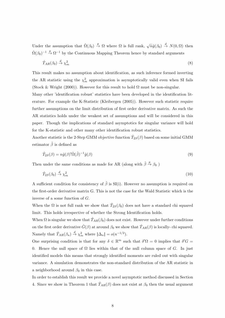
Under the assumption that Ω(β0)p→ Ω where Ω is full rank,

√ng(β0)

d→ N(0,Ω) then

Ω(β0)−1 p→ Ω−1 by the Continuous Mapping Theorem hence by standard arguments

TAR(β0)d→ χ2

m (8)

This result makes no assumption about identification, as such inference formed inverting

the AR statistic using the χ2m approximation is asymptotically valid even when SI fails

(Stock & Wright (2000)). However for this result to hold Ω must be non-singular.

Many other ’identification robust’ statistics have been developed in the identification lit-

erature. For example the K-Statistic (Kleibergen (2005)). However such statistic require

further assumptions on the limit distribution of first order derivative matrix. As such the

AR statistics holds under the weakest set of assumptions and will be considered in this

paper. Though the implications of standard asymptotics for singular variance will hold

for the K-statistic and other many other identification robust statistics.

Another statistic is the 2-Step GMM objective function T2S(β) based on some initial GMM

estimator β is defined as

T2S(β) = ng(β)′Ω(β)−1g(β) (9)

Then under the same conditions as made for AR (along with βp→ β0 )

T2S(β0)d→ χ2

m (10)

A sufficient condition for consistency of β is SI(i). However no assumption is required on

the first-order derivative matrix G. This is not the case for the Wald Statistic which is the

inverse of a some function of G.

When the Ω is not full rank we show that T2S(β0) does not have a standard chi squared

limit. This holds irrespective of whether the Strong Identification holds.

When Ω is singular we show that TAR(β0) does not exist. However under further conditions

on the first order derivative G(β) at around β0 we show that TAR(β) is locally- chi squared.

Namely that TAR(βn)d→ χ2

m where ||∆n|| = o(n−1/2).

One surprising condition is that for any δ ∈ Rm such that δ′Ω = 0 implies that δ′G =

0. Hence the null space of Ω lies within that of the null column space of G. In just

identified models this means that strongly identified moments are ruled out with singular

variance. A simulation demonstrates the non-standard distribution of the AR statistic in

a neighborhood around β0 in this case.

In order to establish this result we provide a novel asymptotic method discussed in Section

4. Since we show in Theorem 1 that TAR(β) does not exist at β0 then the usual argument

8

for inverting statistics to form confidence regions breaks down. As such we slightly gen-

eralize the notion of a confidence set to a Local Confidence Set defined below. A Local

Confidence Set covers a subset of points within a sufficiently small neighborhood around

β0

2.1.1 Local Confidence Sets

We think more generally as providing confidence regions around some point local to β0.

Define a set of Local True Parameters as some ball around β0. Namely define B0(εn) :=

B(β0, εn) (i.e all β ∈ B s.t ||β − β0|| ≤ εn) . A Local Confidence set with size α is as a

set that contains some point (or subset of points ) of the Local True Parameter Set with

probability α. Namely some set C(α) such that ∃β ∈ B0(εn) such that

Prβ ∈ C(α) → α (11)

This idea generalizes the notion of a confidence set. If εn = 0 then B0(εn) = β0 and (11)

is equivalent to the usual definition of a confidence set.

How small a region around β0 that our confidence set covers asymptotically depends upon

the properties T (β).

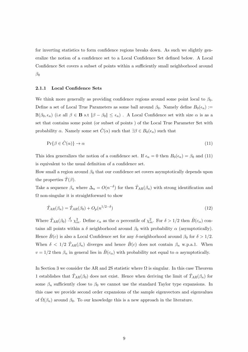
Take a sequence βn where ∆n = O(n−δ) for then TAR(βn) with strong identification and

Ω non-singular it is straightforward to show

TAR(βn) = TAR(β0) +Op(n1/2−δ) (12)

Where TAR(β0)d→ χ2

m. Define cα as the α percentile of χ2m. For δ > 1/2 then B(cα) con-

tains all points within a δ neighborhood around β0 with probability α (asymptotically).

Hence B(c) is also a Local Confidence set for any δ-neighborhood around β0 for δ > 1/2.

When δ < 1/2 TAR(βn) diverges and hence B(c) does not contain βn w.p.a.1. When

v = 1/2 then βn in general lies in B(cα) with probability not equal to α asymptotically.

In Section 3 we consider the AR and 2S statistic where Ω is singular. In this case Theorem

1 establishes that TAR(β0) does not exist. Hence when deriving the limit of TAR(βn) for

some βn sufficiently close to β0 we cannot use the standard Taylor type expansions. In

this case we provide second order expansions of the sample eigenvectors and eigenvalues

of Ω(βn) around β0. To our knowledge this is a new approach in the literature.

9

We show in general that the AR statistic in a neighborhood around β0 has a will have a

χ2m limit under further conditions made in the literature when Ω is not full rank.

We also consider the limit of T2S(β0). In this case Ω(β) exists with probability 1 for all n.

However we show that in general the limit distribution is highly non-standard even with

strong identification.

3 Identification & Singular Variance

The assumption that Ω is full rank is amongst the regularity conditions for various identi-

fication robust statistics to possess a χ2m limit. This assumption is made (if not implicitly)

in all papers regarding identification. Though for a large class of moment functions we

establish that departures from SI lead to Ω being singular.

This is concerning as this literature in general advocates the use of identification robust

methods that do not require the SI condition to hold. However when either of the SI

conditions fail, often so does the condition that Ω is full rank. Hence as it stands the

results in the identification literature robust to identification are robust only to those

identification failures which do not lead to singular moment variance.

Methods of testing a parametric restriction where under the null it is known a priori that

certain parameters are unidentified was considered by Hansen (1996). In this case there

are unidentified parameters under the null and as the unrestricted GMM estimator will

have singular variance.

This problem for testing a specific parameter restriction is side-stepped in Hansen (1996)

by essentially estimating those identified (linear combinations) parameters as a function of

the unidentified parameter. The Wald Statistic is evaluated across (a subset of) the whole

parameter space for the unidentified parameters. A test statistic that essentially integrates

across the unidentified parameters is devised to test the particular null hypothesis. This

removes the unidentified parameters and as such the issue of singular variance is eradicated.

Andrews (1987) provides other examples of singular variance for Wald Type tests of par-

ticular parameter restrictions. Conditions are provided in which replacing the inverse of

the sample variance with a g-inverse has a chi squared limit. In general these conditions

are not satisfied by identification robust statistics.

In spite of this knowledge the issue of singular variance caused by identification failures for

forming identification robust confidence sets has gone unmentioned in the identification

literature. Namely when we do not know a priori whether β0 is strongly identified or not,

10

and/or whether there is singular variance at β0.

The general adage in the identification literature is that the fewer assumptions we make on

identification, the more ‘robust” our inference. However when one assumption is dropped

one must pay attention to the interplay with other assumptions. Namely dropping one

assumption may significantly (or possibly completely) compromise the validity of the re-

maining assumptions.

3.1 Relationship Between Ω and G

In many instances G and Ω are linked. For example casting maximum likelihood as a

GMM estimator then G = Ω via the information equality. In such a case singular moment

variance is equivalent to first order under-identification. The asymptotic distribution of

the Maximum Likelihood estimator and Likelihood Ration statistic in the case where

R(Ω) = p− 1 is provided by Rotnitzky, Cox, Bottai and Robins (2000).

More generally Renault & Donovon (2009) consider the GMM estimator with first-order

under-identification though SI(i) holds. The limit distribution of the GMM Estimator

is not provided though is shown to be non-standard with convergence at rate n1/4 in

directions outside of the null space of G. The limit distribution of the J-Test is derived

when R(G) = p− 1 maintaining the assumption that Ω is full rank.

GMM is consistent though with a non-standard distribution in this case. The limit dis-

tributions in general are impractical and it is not clear how to perform valid inference in

this case. No general limit theory emerges and some knowledge on the form of the under-

identification would be required. More research needs to be carried out on the properties

of GMM estimators with under-identification.

In order to perform valid inference we need to resort to identification robust statistics.

However as we now show first order identification is one common cause of singular variance.

As such we need general theory on identification robust statistics that do not maintain

the non-singular assumption on Ω.

We establish the link between identification failure and singular variance for moment func-

tions derived from conditional moments. This encompasses the a wide class of empirically

used moment functions. More general relationships likely hold between identification and

singular variance and warrant further analysis. Examples are provided in Section 3.2.

11

3.1.1 Conditional Moments

A large class of moment functions considered both theoretically and in practise are derived

from some system of conditional expectations. For example consider some potentially non-

linear residual2 ρi(β) := v(wi, β) where v(·, ·) : K ×B 7−→ R

E[ρi(β)|xi] = 0 (13)

Uniquely at β = β0, for some p× 1 xi.

Define σi(xi) = E[ρi(β0)2|xi] then the optimal instrument f(xi) in the i.i.d case is

f(xi) = E[∂ρi(β0)/∂β|xi]/σi(xi) (14)

Take the simple case where ∂ρi(β0)/∂β is a function only of xi , i.e

E[∂ρi(β0)/∂β|xi] = ∂ρi(β0)/∂β (15)

For example this holds for the class of Non-Linear least squares models.

A simple example is Ordinary Least Squares where wi = (yi, xi) for some scalar random

variable yi where ρi(β) = yi − x′iβ so that ∂ρi(β)/∂β = xi.

In order to use the optimal instrument f(xi) we often have to make some assumptions on

the form of the conditional heteroscedasticity or use some first stage estimate with which

to base inference. Whether we use ∂ρi(β)/∂β as our instrument or ∂ρi(β)/∂β/σi(xi) does

not alter the following relationship between Ω and G.

When σi(xi) is equal to a constant then ∂ρi(β)/∂β is the optimal instrument. Often

∂ρi(β)/∂β is used as an instrument given the form of the conditional heteroscedasticity is

unknown.

The moment function is then

gi(β) = εi(β)∂εi(β)/∂β (16)

For this class of moment functions the Ω and G are

Ω = E[ρi(β0)2∂ρi(β0)/∂β∂ρi(β0)/∂β′] (17)

G = E[∂ρi(β0)/∂β∂ρi(β0)/∂β′] (18)

Hence for any δ ∈ Rp s.t δ′Ωδ = 0 implies that

E[ρi(β0)2(δ′ρi(β0)/∂β)2] = 0 (19)

2For simplicity we consider a scalar residual function. Similar results are easily established for the

scenario of multiple residual functions

12

δ′ρi(β0) = 0 a.s(xi). Therefore δ′Gδ = E[(δ′∂ρi(β0)/∂β)2] = 0. The reverse is also simple

to establish, so that R(Ω) = R(G). First-order under-identification and singular variance

are equivalent.

If we used the optimal instrument then G remains the same though

Ω = E[∂ρi(β0)/∂β∂ρi(β0)/∂β′] = G.

The class of moment functions for which the equivalence holds has been shown for non-

linear least squares and maximum likelihood. A similar link between singular variance

and identification failure likely holds for a broader class of moment functions. This is an

interesting area for future research.

3.2 Examples of Singular Variance

We provide some examples of moment functions with singular variance both with and

without identification failures. Further examples are also introduced and studied in sim-

ulations in Section 5.

3.2.1 Singular Variance with Identification Failure

There are may examples where identification failures lead to singular variance. In essence

many identification failures are linked to some linear combination of moments being re-

dundant at β0. Take for example a class of stochastic semi-linear parametric equations

yi = α′xi + πf(xi, γ) + εi (20)

Define β = (α, π, γ) where α ∈ Rp π ∈ R and γ ∈ Rl for some l > 0.

Where yi is a scalar random variable and xi is a p× 1 vector (for simplicity assumed both

are i.i.d sequence of random variables such that) E[εi|xi] = 0 and E[ε2i |xi] at β = β0 for

some parameter vector β0 = (α0, π0, γ0). Where f(·, ·) : Rp × Rk → R is a continuously

differentiable function. Define εi(β) := yi − α′xi − πf(xi, γ).

∂εi(β)

∂β= (xi, f(xi, γ), π∂f(xi, γ)/∂γ)′ (21)

Then the moment function utilized in Non-Linear Least Squares is

gi(β) = εi(β)(xi, f(xi, γ), π∂f(xi, γ)/∂γ)′ (22)

This is a special class of the class of models considered in Hansen (1996). If we wish to

test for linearity, namely that π0 = 0 then γ0 is unidentified. Hence the GMM estimate

of γ0 will be inconsistent with a random limit distribution. The Wald Statistic (6) will

13

then have a non-standard distribution in this case. Methods to form a test of π0 = 0 are

provided that in general will deliver conservative inference.

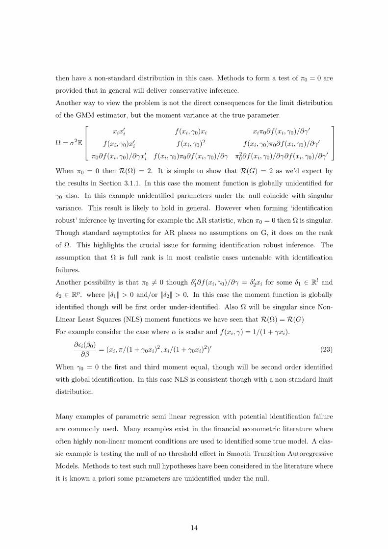
Another way to view the problem is not the direct consequences for the limit distribution

of the GMM estimator, but the moment variance at the true parameter.

Ω = σ2E

xix′i f(xi, γ0)xi xiπ0∂f(xi, γ0)/∂γ′

f(xi, γ0)x′i f(xi, γ0)2 f(xi, γ0)π0∂f(xi, γ0)/∂γ′

π0∂f(xi, γ0)/∂γx′i f(xi, γ0)π0∂f(xi, γ0)/∂γ π20∂f(xi, γ0)/∂γ∂f(xi, γ0)/∂γ′

When π0 = 0 then R(Ω) = 2. It is simple to show that R(G) = 2 as we’d expect by

the results in Section 3.1.1. In this case the moment function is globally unidentified for

γ0 also. In this example unidentified parameters under the null coincide with singular

variance. This result is likely to hold in general. However when forming ‘identification

robust’ inference by inverting for example the AR statistic, when π0 = 0 then Ω is singular.

Though standard asymptotics for AR places no assumptions on G, it does on the rank

of Ω. This highlights the crucial issue for forming identification robust inference. The

assumption that Ω is full rank is in most realistic cases untenable with identification

failures.

Another possibility is that π0 6= 0 though δ′1∂f(xi, γ0)/∂γ = δ′2xi for some δ1 ∈ Rl and

δ2 ∈ Rp. where ||δ1|| > 0 and/or ||δ2|| > 0. In this case the moment function is globally

identified though will be first order under-identified. Also Ω will be singular since Non-

Linear Least Squares (NLS) moment functions we have seen that R(Ω) = R(G)

For example consider the case where α is scalar and f(xi, γ) = 1/(1 + γxi).

∂εi(β0)

∂β= (xi, π/(1 + γ0xi)

2, xi/(1 + γ0xi)2)′ (23)

When γ0 = 0 the first and third moment equal, though will be second order identified

with global identification. In this case NLS is consistent though with a non-standard limit

distribution.

Many examples of parametric semi linear regression with potential identification failure

are commonly used. Many examples exist in the financial econometric literature where

often highly non-linear moment conditions are used to identified some true model. A clas-

sic example is testing the null of no threshold effect in Smooth Transition Autoregressive

Models. Methods to test such null hypotheses have been considered in the literature where

it is known a priori some parameters are unidentified under the null.

14

Another common example the Heckman Selection Model. If the selection bias term con-

tains regressors from the first stage equation and is linear in regressors at the true param-

eter then GMM is first order-underidentified (and possibly globally unidentified). Hence

the GMM estimator will have a non-standard distribution. Also in this case the moments

will have singular variance.

Parametric Semi-Linear models are one class of models where the link between identifica-

tion failure and singular variance is straightforward to see. However this class of models is

by no means exhaustive. The full extent of the relationship between identification failure is

much wider. For example consider the non-linear moments derived using the test-function

approach for interest rate diffusion models . Let rt be the real interest rate where

rt − rt−1 = a(b− rt−1) + εtσrγt (24)

Define β = (a, b, σ, γ) . Under the assumption that εt is stationary at β = β0 where

β0 = (a0, b0, σ0, γ0) Then using the test-function approach of Hansen & Scheinkman (1995)

the following moment functions are derived in Jagannathan & Wang (2002).

gt(β) =

a(b− rt)r−2γ

t − γσ2r−1t

a(b− rt)r−2γ+1t − (γ − 1

2)σ2

(b− rt)r−at − 12σ

2r2γ−a−1t

a(b− rt)r−σt − 12σ

3r2γ−σ−1t

(25)

and has expectations equal to zero at β = β0. Then if σ0 = a0 the third and fourth

moments are equivalent. It is straightforward to show in this case that R(Ω) = R(G) = 3

and hence is both first order underidentified with singular variance.

3.2.2 Singular Variance with Strong Identification

Most common causes of singular variance arise from a lack of identification. However it is

possible that singular variance arises where the moment functions which strongly identify

the true parameter. For example the asset pricing moment equations in Penaranda &

Sentana (2009).

They show that from a set of over-identifying equations 1 linear combination of moments

is redundant at the true parameter. They develop asymptotic theory for the case where

the those combinations of redundant variables for different parameter values are known a

priori.

15

In general we do not know whether moments have a singular variance at the unknown

true parameter. We provide an example where singular moments arise when the moment

functions strongly identify β0. One such example is from linear systems of simultaneous

equations with conditional heteroscedasticity. Consider a simple linear system of equations

ε1i(β1) = y1i − β1xi (26)

ε2i(β2) = y2i − β2xi (27)

Under the assumption that

E[(ε1i(β1), ε2i(β2))′|zi] = 0 (28)

Uniquely at some β10 ∈ R, β20 ∈ R Where zi = (z1i, z2i). In such cases any function of z1i

and z2i is a valid instrument. For simplicity consider the case where the following moment

function is used to identify β0 = (β10, β20)

Equation (29) implies the following moment function

gi(β) =

ε1t(β1)z1i

ε2i(β2)z2i

(29)

Satisfies E[gi(β0)] = 0. (This may not be unique, however it is often implicitly assumed in

applied work that this is the case).

In general the residual εji(βj) interacted with zmli for j = 1, 2 , l = 1, 2 for various poly-

nomial orders m is a valid moment condition. We consider the following simple example

of how singular moments could arise based on such moment functions.

Suppose ε1i(β10) = σ1εiz2i and ε2i(β10) = σ2εiz1i for some σ1 6= 0 and σ2 6= 0 where

E[εi|zi] = 0 and E[ε2i |zi] = 1.

If (ε1i, ε2i, xi, z1i, z2i) is i.i.d then

Ω = E[z21iz

22i]

σ21 σ1σ2

σ1σ2 σ22

(30)

Hence R(Ω) = 1 and hence is singular. G may or may not be full rank and is not impacted

by the conditional heteroscedasticity that leads to Ω being singular.

G =

−E[xiz1i] 0

0 −E[xiz2i]

(31)

G is full rank so long as E[xiz1i] 6= 0 and E[xiz2i] 6= 0. In other words the instruments are

not weak instruments.

16

Many instance of such models arise. For example the C-CAPM implies a set of non-linear

residuals be mean independent of all variables known last period and before. An example

of (26), (27) arise for Conditional CAPM models, Cochrane (1996).

Though the example here is somewhat pathological, when using large systems of equations

interacted with polynomial functions of a potentially infinite set of instruments. It is

entirely plausible that Ω be singular or near-singular in such situations.

In sum the potential for singular moment variance at or near to the true parameter is

prevalent both with and without identification failures. As such the assumption that Ω is

non-singular can not be viewed as a relatively innocuous regularity condition.

4 Asymptotic Theory for Identification Robust Statistics

with Singular Variance

This section derives the asymptotic theory for the Anderson Rubin and 2-Step GMM

Statistics.

Firstly we lay out some definitions for the eigenspaces of the functional matrix Ω(β)

and Ω(β). By construction both matrices are positive definite and symmetric hence the

following decompositions can be made for all β. Let the m×m matrix P (β) be the matrix

of population eigenvalues where

Ω(β) = P (β)Λ(β)P (β)′ = P1(β)Λ1(β)P1(β)′ + P2(β)Λ2(β)P2(β)′ (32)

P (β) := (P1(β), P2(β)), P (β)′P (β) = Im and Λ2(β) = 0. dim(Λ1) = m∗(β) and

dim(Λ2) = m(β) where Λ2(β) is an m(β)×m(β) matrix of zeroes and m = m∗(β)+m(β).

Hence Ω(β) is full rank iff m(β) = 0. Hence Ω(β) =∑m∗

j=1 λ1j(β)P1j(β)P1j(β)′ where

λ1j(β) = [Λ1(β)]jj andP1(β) := (P11(β), P12(β), .., P1m∗(β)) where P1j(β)′P1j(β) = 1 and

λ2j(β) = 0 for j ∈ 1, .., m(β) with eigenvector P2j(β) where P2(β) := (P21(β), .., P2m(β))

where P ′2j(β)P2j(β) = 1 for all j = 1, .., m(β). When referring to the eigenvalues as a

whole we refer to (λ1(β), .., λm(β)) where the first m∗(β) are non-zero eigenvectors and

the final m(β) equal to zero.

We perform a similar decomposition for Ω to express

Ω(β) = P (β)1Λ(β)1P1(β)′ + P2(β)Λ2(β)P2(β)′ (33)

Where P (β) = (P1(β), P2(β)) and P (β)′P (β) = Im and dim(Λ1(β)) = m∗(β) and dim(Λ2) =

m(β). Λ2(β) is a m(β)× m(β) diagonal matrix with the sample estimates of the popula-

tion zero eigenvalues on the diagonal. Λ1(β) is an m∗(β) ×m∗(β) diagonal matrix with

17

sample estimates of the non-zero eigenvalues on the diagonal. P2(β) and P1(β) (where

P1(β) = (P11(β), P12(β), .., P1m∗(β)) and P2(β) = (P21(β), .., P2m(β)) are the correspond-

ing sample eigenvectors.

We are interested in Ω := Ω(β0). For notational simplicity throughout we define P1 :=

P1(β0) and P2 := P2(β0) , Λ1 = Λ1(β0) and Λ2 := Λ2(β0) (hence define m := m(β0), m∗ :=

m∗(β0) as the restive sizes of the two matrices Λ1 and Λ2) where P1 := (P11, .., P1m∗),

P2 := (P21, .., P2m) and for any j [Λ1]jj := λ1j and [Λ2]jj := λ2j .

We firstly show that when Ω has m zero eigenvalues (i.e has rank m − m) then the m

smallest eigenvalues of Ω(β0) are also equal to zero with corresponding eigenvector where

P2 = P2 w.p.1. In this case Ω(β0)−1 does not exist. This is the cause of the breakdown in

standard asymptotic analysis.

Theorem 1 (T1)

When R(Ω) = m− m where m > 0 for all n then Ω is singular for all n the following hold

w.p.1.

(i) Λ2(β0) = 0 (34)

(ii) P2(β0) = P2 (35)

T1 shows that TAR(β) does not exist at β = β0.

In light of T1 evaluate TAR(β) at some sequence βn where nκ∆np→ ∆ where ∆ is a

p × 1 bounded and non-stochastic for any κ > 1/2. We derive the limit distribution of

TAR(βn) and provide conditions under which is has a χ2m limit. As such identification

robust methods based on AR considered in Stock & Wright (2000) and others will provide

valid Local Confidence Sets under these further conditions, containing all such sequences

βn asymptotically with a certain probability.

Using the eigen-decomposition of Ω(β) we can express

TAR(βn) = ng(βn)′P (βn)Λ(βn)−1P (βn)g(βn) (36)

= g(βn)′P1(βn)Λ1(βn)−1P1(βn)′g(βn)+ g(βn)′P2(βn)Λ2(βn)−1P2(βn)′g(βn) (37)

Higher order expansions of Λ2(βn) and P2(βn) around β0 are derived. When m > 0 (i.e Ω

is singular) then Λ2(β0) = 0. Hence higher order terms in the expansion of the eigenvalues

Λ2(βn) around β0 enter first-order asymptotics of TAR(βn). Amazingly under some further

conditions on G then the AR statistic retains a standard chi squared limit locally around

β0.

18

Using the expansions of sample eigenvalues/vectors around β0 we show under certain

conditions that

nκ+1/2P ′2g(βn)d→ N(0, D) (38)

n2κΛ2(βn)p→ D (39)

For some full rank matrix non-stochastic matrix D .Hence

ng(βn)′P2(βn)Λ2(βn)−1P2(βn)′g(βn)d→ χ2

m (40)

So TAR(β) is locally chi-squared in a δ-neighborhood around β0.

Matters become more involved for T2S(β0). We consider the case where β the initial

estimator is strongly consistent. In this case βn = β where β is some initial GMM

estimator. In this case n1/2∆n = n1/2(β − β0) has a limit Gaussian distribution In this

case it is shown that nΛ(β) has a random limit. This is the cause of the breakdown of

standard asymptotics for 2S-GMM.

As such the limit distribution of T2S(β0) will depend upon the distribution of β. Asymp-

totics for T2S(β0) with identification failure is beyond the scope of this paper and may

prove impractical in general.

4.1 Asymptotic Expansions of Perturbations of Ω(β) around β0

Singularity of Ω poses a theoretical challenge to deriving asymptotic expansions of both

quadratic objective functions as a function of the inverse of some sample estimate of Ω.

Essentially we wish to expand Ω(βn)−1 . However Ω(β0)−1 doesn’t exist. As such we

cannot use Taylor Type expansions commonly used to derive the higher order expansions

of various test statistics.

We derive an expansion of both the AR and 2S statistic by providing expansions for

the eigenvectors and eigenvalues of Ω(βn) around β0. This approach is to the best of our

knowledge new in the identification literature and is of theoretical interest in its own right.

We expand λj(βn) and Pj(βn) around β0 for j = 1, ..,m. This result will prove crucial

in deriving the limit distribution of the 2-Step and AR objective function along with tests

of singularity.

These results are of interest in their own right and will be a useful framework for deriving

asymptotic theory for moment type estimators, tests of identification and other important

statistics based on moments have singular variance.

19

Assumption 1 (A1) (i) wi(i = 1, , , n) independent ∀ i,n (ii) minj λ1j > c for some c > 0

(iii) ||Ω(β0)− Ω|| = Op(n−1/2) , (iv)|| 1n

∑ni=1(Gi(β

∗)−Gi(β))|| ≤ M ||β∗ − β0||) ∀β, β∗ ∈ B

where M = Op(1), (v) ||Ω(β∗)− Ω(β)|| ≤ M ||β∗ − β0||) ∀β, β∗ ∈ B where M = Op(1) (vi)

m <∞ (vii) ||Ω(β0)|| = Op(1), (viii) ||G(β0)|| = Op(1),

A1(i) could be dropped to allow dependence, however we would need to use more general

estimators of Ω for example HAC. Extensions to this case are relatively straightforward

under further regularity conditions though would do little to change the main results of

this paper. A1 (ii) is relatively innocuous and maintains that the non-zero eigenvalues are

bounded away from zero for all n.

A1 (iii) is stronger than necessary and assumes that the sample variance Ω(β0) is strongly

consistent. The rate could be weakened and the main results below would not funda-

mentally alter. A1(iv), (v) are continuity assumptions on Ω(β) and G(β). A1 (vii),

(viii) assume that the sample variance and first order derivative at β0 are asymptotically

bounded. For simplicity we assume that m is fixed in A1 (vi). Extensions to m growing

with the sample size would be relatively straightforward.

A strong set of sufficient conditions for A1 is that wi is i.i.d, Gi(β) and gi(β) are continuous

and bounded in a neighborhood of β0 for all i, n.

When Ω is singular T1 establishes that λ2j(β0) = 03. As such higher order terms in the

expansion of λ2j(βn) and P2j(βn) around β0 enter the first order asymptotics of both the

AR and 2S statistic at β0.

Theorem 2 derives asymptotic expansions for the sample eigenvectors and eigenvalues of

Ω(βn) around β0. Higher order expansions are provided only for λ2j(βn) and P2j(βn).

The higher order terms in the expansion of λ1j(βn) and P1j(βn) do not enter first order

asymptotics for AR or 2S. For brevity only first order expansions for P1j(βn) and λj(βn)

are provided. Though not explicitly provided, higher order expansions could also easily

be derived for λ1j(βn) and P1j(βn) using the proof of T2.

These results are of interest in themselves and may prove useful for deriving general asymp-

totic theory with singular variance in other non-standard settings.

Theorem 2a (T2a) Under A1

i P1j(βn) = P1j(β0) +Op(||∆n||) ∀j = 1, ..,m∗3In the following any sample eigenvector or eigenvalue with an arbitrary subscript j means the results

hold for all such j. So that for example λ2j(β0) = 0 means the result holds for all j = 1, ..m

20

ii P2j(βn) = P2j + P1(β0)Λ−11 P1(β0)′(Ω(βn)− Ω(β0))P2j +Op(|||∆n||2) ∀j = 1, .., m

By standard arguments we can show that P1(β0) and Λ(β0)−1 converge to P1 and Λ1 at

rate n1/2 under A1 (ii), (iii). (Theorem 4.2, Bosq (2000)). Also by T1 Ω(β0)P2j = 0.

Then it is straightforward to establish

Corollary 1 (C1). Under A1 then T2a implies that

i P1j(βn) = P1j +Op(n−1/2 ∨ ||∆n||)

ii P2j(βn) = P2j + P1Λ−11 P ′1Ω(βn)P2j +Op(||∆n||(n−1/2 ∨ ||∆n||)))

Define the following,

γjn = P ′2j1n

∑ni=1G

′i∆n∆′nGiP2j ,Ψjn := Λ

−1/21 P ′1

1n

∑ni=1 gi∆nG

′iP2j , ψjn := Ψ′jnΨjn and

υjn := γjn − ψjn for j = 1, .., m.

Theorem 2b (T2b) Under A1

i λ1j(βn) = λ1j +Op(n−1/2 ∨ ||∆n||)

ii λ2j(βn) = υjn +Op(||∆n||2(||∆n|| ∨ n−1/2)

T2a and b are crucial for deriving the limit distribution of TAR(βn) (and also T2S(β0)).

Section 4.2 provides asymptotic theory for the AR and 2S GMM using the higher order

expansions in T2a and T2b.

4.1.1 Limit Distribution of Identification Robust Statistics

Using T2a and T2b we can derive the limit distribution of both TAR(βn) and T2S(β0). We

derive the limit of TAR(βn) and not TAR(β0) as noted in T1 TAR(β0) does not exist when

Ω is not full rank.

4.1.2 Anderson Rubin Statistic

We firstly derive the limit distribution of TAR(βn) for some sequence βn. In this case we

consider a sequence βn where nκ∆np→ ∆ where ∆ is a non-stochastic p× 1 vector. Define

for j = 1, ..m

Φj := Λ−1/21 P ′1E[

1

n

n∑i=1

gi∆′G′iP2j ] (41)

21

ψj := Φ′jΦj (42)

γj := E[1

n

n∑i=1

P ′2jG′i∆∆GiP2j ] (43)

Assumption 2 (A2) (i)nκβnp→ ∆ where ∆ is a p× 1 non-stochastic vector and κ > 1/2,

(ii)√n(G(β0) − G)′v

d→ N(0,Kv) where Kv := 1n

∑ni=1(E((Gi − G)′vv′(Gi − G)) for any

v ∈ Rp. (iii)√ng(β0)

d→ N(0,Ω), (iv) δ′Ω = 0 =⇒ δ′G = 0 for δ ∈ Rp (vi)nκγjnp→ γj ,

nκψjnp→ ψj

A2(i) assumes that the sequence nκβn has a non-random limit. This assumption could be

extended to allow for different rates of convergence for difference linear combinations of

parameters βn, however this would not change the result. The assumption this sequence

has a non-stochastic limit is innocuous since for AR when inverting to form a confidence

set βn is fixed. Unlike 2S below where the weight matrix is evaluated at an estimator of β0

where in this case n1/2∆n has a random limit under the assumption the initial estimator

is strongly identified.

A2(ii) is a high level assumption that a Central Limit Theorem holds for the matrix

n1/2(G(β0) − G), similarly for A2 (iii) regarding n1/2g(β0). The limit variance does not

allow for dependence in G(β0)−G since for simplicity we have assumed wi is independent

over i and hence so is Gi. A2 (iv) makes a high level weak law of large numbers assumption,

given that nκ∆np→ ∆ then nκψjn converges to ψj assuming a weak law of large numbers

results holds.

A key assumption is A2 (iv) that the null space Ω belongs to the null column space of

G. In just-identified settings, m = p then A2(iv) rules out strongly identified moment

conditions. This may also hold for m > p. Hence when there is singular variance, in order

for the AR statistic to satisfy Theorem 3 then the moment function must in many cases

also be first order under identified. This is a startling result, namely that if Ω is singular

and G is full rank (i.e is first order identified) then the AR statistic is not in general

locally-chi squared.

In fact in Simulation 1 an example of this case we demonstrate the AR statistic in a 1/n

neighborhood of β0 is highly non-standard. Hence the AR statistic is not necessarily robust

to singular variance when there is strong identification. This goes against the commonly

held wisdom of the identification literature. This paper is a first step in understand the

complex relation between usual notions of identification and regularity conditions often

relegated to secondary importance.

22

Theorem 3 Under A1-A2

TAR(βn)d→ χ2

m (44)

Hence inverting TAR(β) using the χ2m approximation will provide asymptotically valid

confidence regions for any δ−neighborhood around β0 and hence will be a Local Confidence

Set. Essentially inverting the AR statistic by the usual method will contain any β an

infinitesimally small distance away from β0 with the correct probability asymptotically.

However Assumption 2 must hold. Dropping the assumption that Ω is full rank we require

a central limit theorem to hold for G(β0) − G and that the null space of Ω to lie in the

null space of G.

4.1.3 2-Step GMM Statistic

For 2-Step GMM βn = β where ∆n = β−β0 and when appropriately scaled has a random

limit. We consider the case where the initial estimator is strongly identified so that n1/2∆n

in this case has a Gaussian limit distribution. Extensions to allow for departures from

strong identification would prove extremely difficult and are beyond the scope of this

paper.

For the AR statistic the sequence ∆n was fixed and as we saw under extra conditions this

statistic retained the standard chi squared limit in a neighborhood of β0. This is not the

case for 2-Step GMM. the distribution of β enters the limit distribution of T2S(β0) even

when β is strongly identified. It is shown below this distribution has a complicated form.

Define the following Υ := ΣP1Λ1/21 and Σ is defined in A3(i) where for all j = 1, ..m

and h = 1, ..,m∗

Πjn = Υ1

n

n∑i=1

(G′iP2jP′2jGi −

1

n

n∑j=1

G′jP′2jP2jGi(g

′iP1Λ−1

1 P ′1gj))Υ′ (45)

Πj = ΥE[1

n

n∑i=1

(G′iP2jP′2jGi −

1

n

n∑j=1

Ξ′G′jP′2jP2jGi(g

′iP1Λ−1

1 P ′1gj))]Υ′ (46)

Θhjn := λ−1/21h

n∑i=1

g′iP1hP′2jGiΥ (47)

Θhj := λ−1/21h E(

n∑i=1

g′iP1hP′2jGi)Υ (48)

23

Where Θhj is a 1×m∗ vector where Θhj := (θhj1, .., θhjm∗)

Assumption 3 (A3) (i) (β − β0) = Σg(β0) + op(1) for a full rank p ×m matrix Σ, (ii)

Πjnp→ Πj ∀j = 1, .., m, (iii) Θhjn

p→ Θhj ∀j = 1, .., m, h = 1, ..,m∗

Define W be a m∗ ×m∗ random matrix with a standard Wishart distribution.

By A3(i) and A2(ii)

√n(β − β0)

d→ ΥZ (49)

Where Zd∼ N(0, Im∗) since P ′2g(β0) = 0. Define Z : (Z1, .., Zm∗)

′

Theorem 4(i) derives the limit distribution of λ2j(β) which will be useful in both deriv-

ing the limit distribution of T2S(β0) and also for deriving tests of the rank of Ω in Section 5.

Theorem 4 (T4) Under A1-A3

λ2j(β)d→ tr(ΠjW) (50)

Theorem 5 (T5) Under A1-A3

T2S(β0)d→

m∗∑k=1

Z2k +

m∑j=1

(m∗∑h=1

m∗∑l=1

θhjlZlZh)2/tr(ΠjZZ′) (51)

T5 shows the highly non-standard limit distribution of T2S(β0) when m > 0, i.e moments

have singular variance. When m = 0 then T5 shows that T2S(β0) has a χ2m limit dis-

tribution. With singular variance the 2S statistic with strong identification is a highly

non-linear function of m∗ independent standard normal random variables.

T4 can be used to test the rank of Ω. This is the case only when GMM is strongly

identified. With departures from strong identification the limit distribution of the GMM

estimator in general has non-standard rates of convergence to a non-standard distribution.

With lack of global identification in general moment type estimators are inconsistent. This

causes obvious issues for testing the rank of Ω(β) and β = β0, i.e the rank of Ω.

In general inverting the 2S statistic using a standard χ2m limit provides incorrect inference.

Modified methods of inference based on the 2S statistic are derived, though are robust

only to certain forms of identification failure.

The message which follows from this, is that inverting the AR statistic, under further

conditions than those posed in the literature will still provide valid inference with general

identification failures. Not just departures of strong identification but also to non-singular

24

variance which we argue is a third identification condition which cannot be made separately

given the discussion on the interplay between identification and singular variance in Section

3.

One peculiar case which emerges is when strong identification occurs with singular vari-

ance. In many cases this will invalidate A2 (ii) and in general AR will not have a locally

chi squared limit. As such methods which remove eradicate the singularity issue would

be preferable. This is especially the case as in a simulation when moments have almost

singular variance with strong identification the AR statistic is poorly approximated by a

χ2m limit.

Further investigations in to the link between singular variance, identification and methods

to provide robust asymptotically valid inference are greatly needed. Inverting the AR

statistic using a χ2m limit is not as innocuous as implied by the identification literature

once we view the full rank assumption on the variance of the moments as an identification

condition

5 Singularity Robust Confidence Sets

Using Theorem 4 we can derive a test for the rank of Ω in the case when β is strongly

identified. Deriving a test with global or first order identification is beyond the scope of

this paper.

We may also wish to perform formal statistical tests of the rank of Ω. Theorem 2 derives

the limit distribution of the sum of the n times the r smallest eigenvalues under the null

that m∗ = r

Theorem 4 naturally lends itself to testing the null hypothesis that the rank of Ω is m− r

for any 1 ≤ r < m (i.e to test the Null Hypothesis that m = r). Section 5.2 details

how to perform such tests and estimate the quantiles of tr(ΨjW) in practice. Simulation

experiment 1 verifies the validity of this asymptotic approximation.

5.1 Testing for redundant moments in non-linear models

Given the invalid approximation of T2S(β0) by χ2m when the variance of moments is singular

(and poor approximation when β0 is almost a point of a singularity) we’d like some method

of testing for the rank of Ω. When Ω is not a function of β then if Ω is not full rank then

it will imply that Ω is also singular for any n.

Suppose we wish to test the following Null Hypothesis.

25

H0 : R(Ω) = m− r (52)

H1 : R(Ω) > m− r (53)

Where 0 < r < m. Under the null then

n

r∑j=1

λ2j(β)d→ tr(

r∑j=1

ΠjW) (54)

We require estimates of P1P′1, P2P

′2 and Υ along with an initial estimator β0 to esti-

mate each Πj . We take β to be the initial GMM estimator with (possibly data de-

pendent) matrix W . In this case when GMM is strongly identified then A3(ii) is sat-

isfied with Σ = (G′WG)−1G′W and a consistent estimate can be formed using Σ =

(G(β)′WG(β))−1G(β)′W

Though P1 and P2 are not in general continuous function of the elements of Ω, P1P′1

and P2P′2 are , Kato (1982). Hence since by T2 P1

p→ P1 P2p→ P2 then by the CMT

P1P′1

p→ P1P′1 and P2P

′2

p→ P2P′2.

Hence we can take an estimate of Πj based upon Σ, P1(β), P2(β) and Λ and β. Then

under A1-A3 it is straightforward to show that Πjp→ Ψj .

We can then simulate the distribution of tr(∑r

j=1 ΠjW) by taking B draws from r uncor-

related standard normal variables Z∗b where Z∗bd∼ N(0, Ir) for b = 1, ..B and taking the

α% quantiles of tr(ΨW∗b ) where W ∗b = Z∗bZ

∗′b . Since W∗ approximates the distribution

of W with arbitrary precision for B → ∞ and∑r

j=1 Πjp→∑j = 1rΠj by A1( it is easy

to establish that qαp→ qα where

qα = infx ∈ R : Prtr(r∑j=1

ΠjW∗) ≤ x ≥ α (55)

qα = infx ∈ R : Prtr(r∑j=1

ΠjW) ≤ x ≥ α (56)

Though in simulations the size of the test is poorly sized for even moderately large sam-

ple sizes, the power of the test is very strong. Under the alternative hypothesis then

n∑r

j=1 λ2j(β) diverges at rate n such that when the null is not true.

26

5.2 Estimates of Rank w.p.1

We could use this result to formulate some cut off point with which to select the number

of non-zero eigenvalues of Ω which would correctly determine the rank of Ω asymptotically

w.p.1. For example letting r := infj≥0(λj > δn) where δn > 0 and Theorem 3 of Bathia,

Yao & Ziegelmann(2010) shows that Prr = m → 1 as n→∞ when (δ2nn)−1 → 0.

This result is extremely useful to modify the 2-Step GMM objective function to remove

the potential problem of Ω being singular. The next section shows that when Ω is singular

that T2S(β0) is bounded in probability though in general will no longer be distributed χ2m.

If we take our estimator r then since r = m asymptotically w.p.1 we can delete redundant

moments using the estimated eigenvectors such that the modified set of moments satisfies

standard asymptotic theory asymptotically. No estimation error from estimating m feeds

in to the limit distribution of the transformed objective function asymptotically. Namely

we derive an objective function based on a set of moments that have non-singular variance

with rank m∗.

There are two possible ways to correct for the non-standard limit distribution of T2S(β0).

The first method is to estimate m using the method detailed to remove redundant combi-

nations of moments. The second method is to use bootstrap critical values with which to

invert T2S(β) to form a confidence region that is singularity-robust.

5.3 Removing Redundant Combinations of Moments

Given an estimate of r s.t Prr = m = 1 as n→∞ then the modified two step criterion

function T r2S(β0)

T r2S(β) :=m−r∑j=1

(P ′j√ng(β))2λ−1

j (57)

Utilizes the first m − r moments P ′j g(β) that have the largest eigenvalues. Given an

estimator r such that Prr = m → 1 then for any c > 0

PrT r2S(β0) ≤ c → PrT ∗2S(β0) ≤ c (58)

as n → ∞ where T ∗2S(β0) =∑m∗

j=1(P ′j√ng(β0))2λ−1

j Since m − r = m − m = m∗ with

probability 1 as n → ∞ and since√ng(β0) = Op(1) by A2(ii) and λj = λj + Op(n

−1/2)

for and Pj = Pj +Op(n−1/2) j ∈ 1, ..,m∗ (i.e for those j where λj > 0 by T2/

Then by A2(ii)√ng(β0)

d→ N(0,Ω) where Ω = P1Λ1P′1 . Hence (P ′1j g(β0)/λ

1/21j )2

dN(0, 1)

for j ∈ 1, ..,m∗. Therefore T ∗2S(β0)d→ χ2

m∗ .

27

This establishes then that for any c > 0 and as n→∞

PrT r2S(β0) ≤ c → Prχ2m∗ ≤ c (59)

Hence we can then derive confidence regions for β0 with valid levels asymptotically though

using the modified 2 Step GMM function T r2S(β) and the quantiles of χ2m∗ . We do not know

m∗ however since Prr = m → 1 then the quantiles of χ2m−r will be valid asymptotically.

Note that this method will yield confidence regions with correct size the case even if

m∗ < p. Though the smaller is m∗ the wider will our convergence regions become, though

will still be correctly sized asymptotically.

Another method would be to work directly with T2S(β) using quantiles based on a boot-

strap method without deleting redundant moments. The drawback is it is difficult to pro-

vide the validity of a bootstrap theoretically. The benefit is that we do not need to remove

redundant moments which may be overly conservative in small samples. The bootstrap is

shown to work well in simulations, even when the GMM estimator is under-identified and

hence A1(i) breaks down Renault & Donovon (2009).

Theorem 4 derives the limit distribution of the 2S statistic and may prove useful in proving

the validity of the bootstrap, at least in the case where GMM is strongly identified.

5.4 Bootstrap Confidence Regions

Bootstrapping robust statistics has received relatively little attention in the literature.

Kleibergen (2011) derive bootstrap critical values for the identification robust statistics in

Kleibergen (2005). For example for the Continuous Updating Estimator and the Kleiber-

gen Statistic and others. This paper does not derive higher order expansions for the 2-Step

GMM estimator. Also Kleibergen (2005) made the assumption that Ω is non-singular for

any n and hence that the minimum eigenvalue is well separated from zero for all n.

Establishing the validity of the bootstrap method for the 2-Step GMM objective function

when Ω is singular would be difficult even if the GMM estimator were strongly identified.

The limit distribution of the 2-Step GMM depends upon the limit distribution of the

sample estimates of the zero eigenvalues, which by Theorem 4 shows this distribution to

be highly non-standard. We do not provide conditions under which or the validity of

the bootstrap method. However we highlight a method similar to that put forward in

Kleibergen (2011) used when Ω is singular. It is shown to work well in simulations in

Section 6.

28

For any β ∈ B define gi(β) = gi(β)− g(β). Take a bootstrap sample of size N with replace-

ment from gi(β) to form a bootstrap sample b g∗1b(β), .., g∗nb(β) for b = 1, .., B∗ Then

define the bootstrapped 2-Step GMM objective function at β Tnb(β) := g∗(β)′bΩ∗b(β)g∗(β)b

Where Ω∗b(β) =∑n

i=1 gib(β)gib(β)′

Define T2S(β) = ng(β)′Ω(β)−1g(β). Take then the α∗ quantile of Tnb(β) from the boot-

strap sample which we define as α(β) and perform the inversion of T2S(β) selecting all

β ∈ B such that T2S(β) ≤ α(β). At β0 then α(β0) should asymptotically approximate the

quantiles of T2S(β0) (which is verified in three simulations. For β 6= β0 then T2S(β)→∞

under strong identification. With weak identification, or in the worse case scenario total

lack of identification then the power properties may be poor. Just as would be the case

of inverting robust-statistics in the case where Ω is singular, Dufour (1997), Kleibergen

(2005).

6 Simulations

We consider two different ways in which singularity and near- singularity may arise. Sim-

ulation 1 and two both consider instrumental variable models where the first stage is a

non-linear regression. This approach is common when the endogenous variable is a binary

variable, for example Angrist (2001). For example it isn’t uncommon for a first stage

Probit of Logit to be run in these cases. Simulation 1 considers the case where the GMM

estimator is strongly identified, though through conditional heteroscedasticity the moment

functions are singular at β0.

We also consider the case where the variance of the moments is almost singular, i.e where

the determinant of Ω is very small. In the former case the distribution of nQ2S(β0) does

not converge to a chi squared limit , though is bounded, even for large n, as to be expected

by Theorem 4. The case where Ω is almost singular, for small to medium sample sizes the

chi squared approximation is poor, with the distribution of T2S(β0) eventually been well

approximated by a chi squared distribution. In this example since the GMM Estimator is

strongly identified, we can use Theorem 2 to derive the limit distribution of the smallest

eigenvalue which is zero. The approximation of the limit distribution in Theorem 2 is

quite poor, though eventually converges for large sample size. We also show the bootstrap

confidence regions to perform well.

Simulation 1 satisfy A3 since Ω is singular whilst G is full column rank and hence first-

order identified. In this case we show that TAR(βn) for βn = β0 + 1/N has a non standard

29

chi squared distribution for any local sequence around β0. It is beyond the scope of this

paper to derive the limit distribution of TAR(βn) with singular variance where first order

identification is maintained.

Simulation 2 considers a parameter semi linear regression model used in Bierens (1990) to

test for non-linearities. For certain parameter values there is a lack of global identification

which causes issues for testing for non-linearities Hansen (1996). It is also the case that

the moment variance matrix would be singular for these parameter values which will cause

issues even for those statistics robust to identification failures. There exist some parameter

values where though globally identified, there is first order under-identification as well as

singular variance.

In this case the GMM estimator is consistent though with a non-standard distribution.

This would invalidate parameter inference based on the normal approximation to the

GMM estimator. Also from confidence intervals based upon the Wald , LR or Likelihood

ratio statistic based on an initial estimate of β0. The 2-step GMM objective function does

not require first order identification in order to provide correct inference on β0, requiring

only the initial estimator be evaluated at the true parameter is shown to be non-standard.

In this case the distribution of the estimated smallest eigenvalue is uncertain, however

we can show using theorem 2b(ii) in this case that it is Op(n−1/2) with a non-standard

distribution. We consider β0 where there the variance of the moments is singular and near

singular. In the latter case, convergence to the standard chi squared limit is shown to be

very slow.

Simulation 2 does satisfy the conditions of A3 and hence Theorem 3 holds and the con-

vergence of TAR(βn) for βn = β0 + 1/n to a χ2m limit is demonstrated.

6.1 Simulation 1: Non-Linear Simultaneous Equations with Conditional

Heteroscedasticity

Let (yi, xi, zi) i = 1, .., n be an i.i.d sequence where

yi = θ0xi + εi (60)

xi = (1 + π0zi)−1 + vi (61)

Where both E[εi|zi] = 0 an E[vi|zi] = 0] for all i.

Define β = (θ, π), then the moment function

gi(β) =

((yi − θxi)(1 + πzi)

,(xi − (1 + πzi)

−1)zi(1 + πzi)2

))′ (62)

30

E[gi(β0)] = 0 (63)

Where β0 := (θ0, π0)/ The second moment condition is from the non-linear regression

in (53). First moment condition uses the optimal non-linear instrument with which to

identify β0. Here π0 is a nuisance parameter and not the variable of interest.

Ω(β0) := E[gi(β0)gi(β0)′] = E

E[ε2i |zi](1+πzi)2

E[εivi|zi]zi(1+πzi)3

E[εivi|zi]zi(1+πzi)3

E[v2i |zi]z2i(1+πzi)4

Suppose the process (εi, vi) i = 1, .., n satisfies the following

εi|ziiid∼ N(0, σ2

ε (1 + π0zi)2z−2i ) (64)

vi|ziiid∼ N(0, σ2

v(1 + π0zi)4z−4i ) (65)

E[εivi|zi] = ρσvσεz−1i (1 + π0zi)

3 (66)

Where ρ = cor(εi, vi) Hence E[ε2i |zi] = σ2ε (1 + π0zi)

2z−1i

E[v2i |zi] = σ2

vz−2i (1 + π0zi)

4

Ω(β0) =

σ2ε ρσvσε

ρσεσv σ2v

(67)

p = 1 implies singular moments, p ≈ 1 then Ω is almost singular.

We simulate a sample of ((yi, xi, zi, εi, vi) i = 1, .., n satisfying (52)-(53) an (56)-(58)

letting zi = abs(ei) + 0.1 where ei i.i.d N(0, 1) and setting π0 = β0 = 0.1 , σε = σv = 1

with number of repetitions R = 20000 for each case.

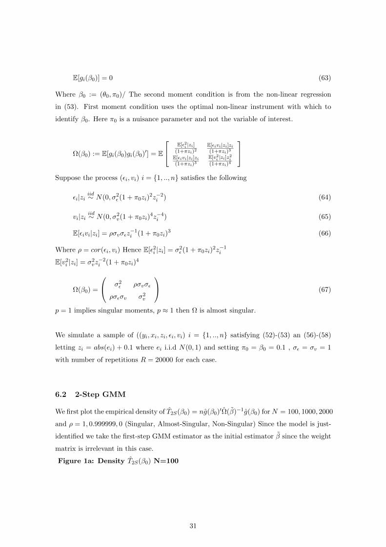
6.2 2-Step GMM

We first plot the empirical density of T2S(β0) = ng(β0)′Ω(β)−1g(β0) forN = 100, 1000, 2000

and ρ = 1, 0.999999, 0 (Singular, Almost-Singular, Non-Singular) Since the model is just-

identified we take the first-step GMM estimator as the initial estimator β since the weight

matrix is irrelevant in this case.

Figure 1a: Density T2S(β0) N=100

31

Figure 1b: Density T2S(β0) N=1000

Figure 1c: Density T2S(β0) N=2000

32

Under A2(ii) that√ng(β0)

d→ N(0,Ω) then when moments have non-singular variance,

i.e R(Ω) = 2 (i.e non-singular) then T5 with m = 0 and m = 2 (i.e standard asymptotics)

then T2S(β0)d→ χ2

2

Where Prχ22 ≤ 5.99 = 0.95 Prχ2

2 ≤ 9.21 = 0.99

Table 1 plots the 90% and 95% quantiles for each n,p.

Table 1: Small Sample Quantiles of T2S(β0)

N = 100 N = 1000 N = 2000

q = 0.95 q = 0.99 q = 0.95 q = 0.99 q = 0.95 q = 0.99

ρ = 1 77.37 4355 18.2 38.22 17.3 33.34

ρ = 0.99999 41.9 1245 7 14.03 6.41 11.28

ρ = 0 14.98 311 6.09 9.84 6.02 9.32

Fig 1a-c show that case where the moments are uncorrelated (p=0) the χ22 provides a

reasonable approximation for small N (N = 100) and extremely good for (N=1000,2000).

For almost singular, the χ22 approximation is poor for small and medium sample size though

is reasonable for large N (N=2000). When moments are singular at β0 the distribution

does not converge to a χ22, though is bounded, which corresponds with Theorem 2. The

quantiles are roughly more than double those of a χ22 when p = 1. To visualise this we

plot the Quantile-Quantile plots of T2S(β0) and χ22 in Fig 2a-c.

Fig 2a: Quantile-Quantile Plots of T2S(β0) and χ22 N = 100

33

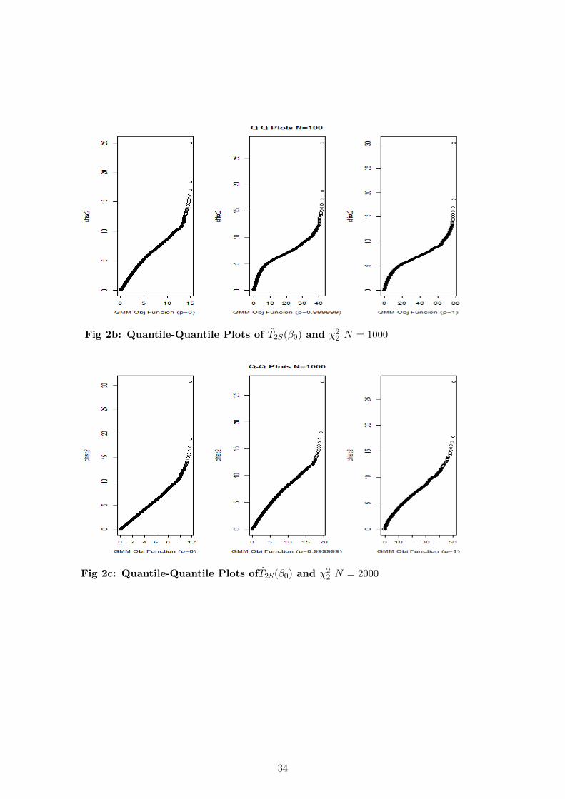
Fig 2b: Quantile-Quantile Plots of T2S(β0) and χ22 N = 1000

Fig 2c: Quantile-Quantile Plots ofT2S(β0) and χ22 N = 2000

34

Again we see that when p = 1 even for N = 2000 the chi22 approximation is massively

undersized. Performing the simulation for N = 20000 I found a similar result, though the

result is not reported here.

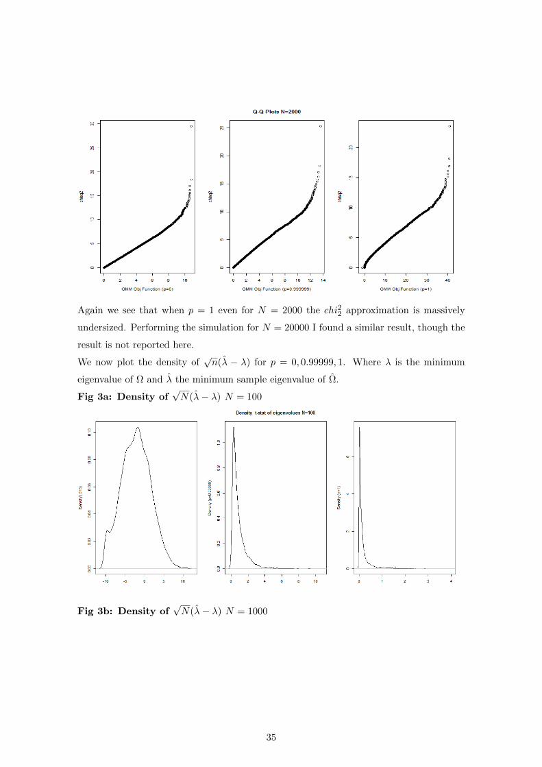
We now plot the density of√n(λ − λ) for p = 0, 0.99999, 1. Where λ is the minimum

eigenvalue of Ω and λ the minimum sample eigenvalue of Ω.

Fig 3a: Density of√N(λ− λ) N = 100

Fig 3b: Density of√N(λ− λ) N = 1000

35

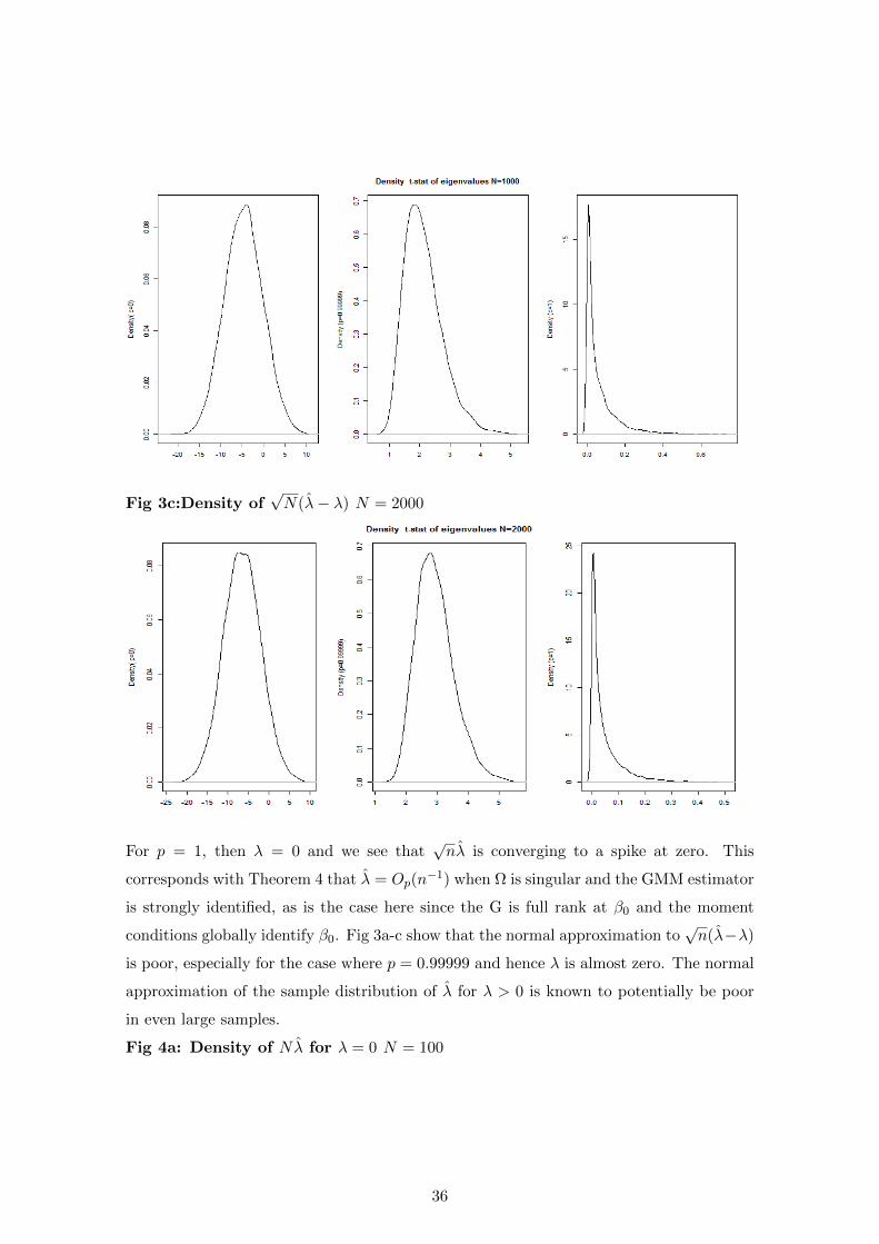
Fig 3c:Density of√N(λ− λ) N = 2000

For p = 1, then λ = 0 and we see that√nλ is converging to a spike at zero. This

corresponds with Theorem 4 that λ = Op(n−1) when Ω is singular and the GMM estimator

is strongly identified, as is the case here since the G is full rank at β0 and the moment

conditions globally identify β0. Fig 3a-c show that the normal approximation to√n(λ−λ)

is poor, especially for the case where p = 0.99999 and hence λ is almost zero. The normal

approximation of the sample distribution of λ for λ > 0 is known to potentially be poor

in even large samples.

Fig 4a: Density of Nλ for λ = 0 N = 100

36

Fig 4b: Density of Nλ for λ = 0 N = 1000

Fig 4c: Density of Nλ for λ = 0 N = 2000

37

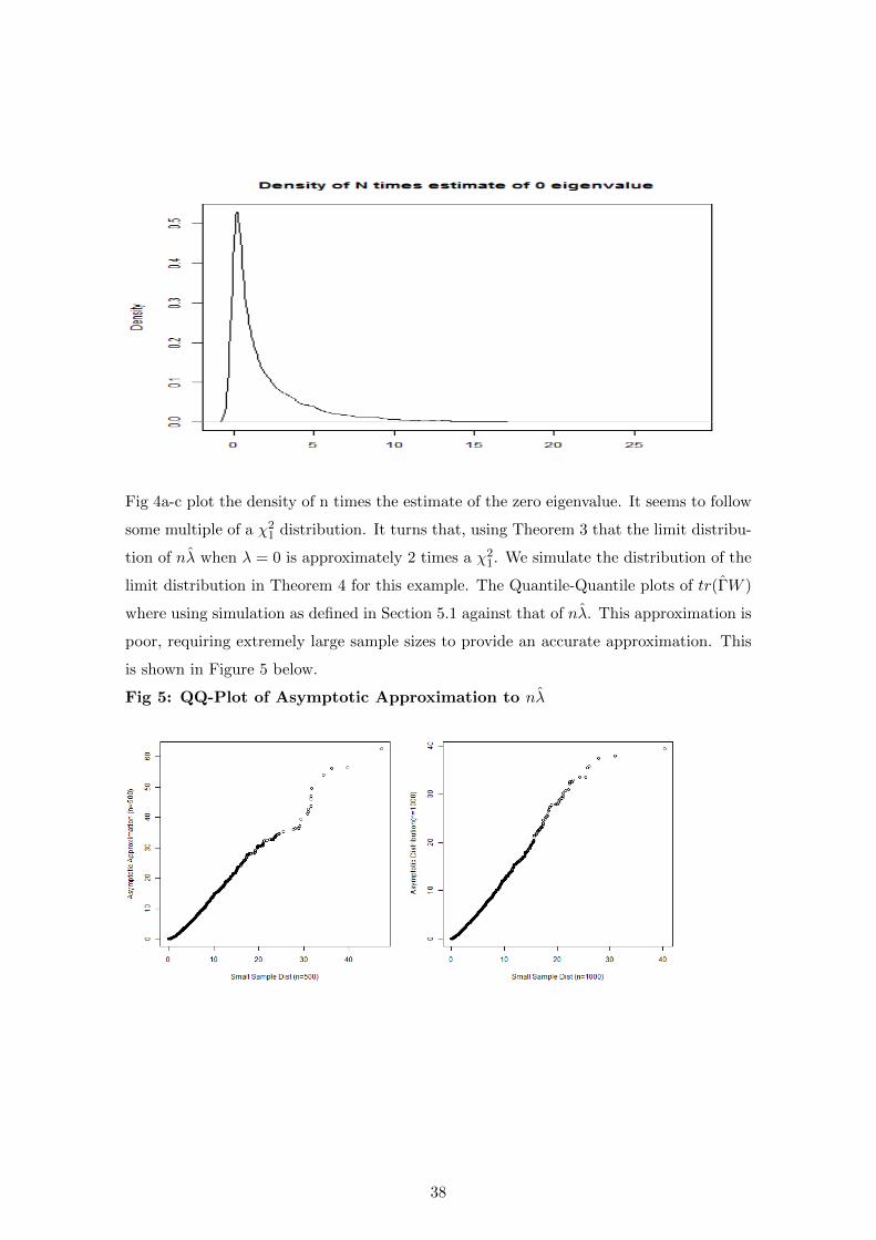
Fig 4a-c plot the density of n times the estimate of the zero eigenvalue. It seems to follow

some multiple of a χ21 distribution. It turns that, using Theorem 3 that the limit distribu-

tion of nλ when λ = 0 is approximately 2 times a χ21. We simulate the distribution of the

limit distribution in Theorem 4 for this example. The Quantile-Quantile plots of tr(ΓW )

where using simulation as defined in Section 5.1 against that of nλ. This approximation is

poor, requiring extremely large sample sizes to provide an accurate approximation. This

is shown in Figure 5 below.

Fig 5: QQ-Plot of Asymptotic Approximation to nλ

38

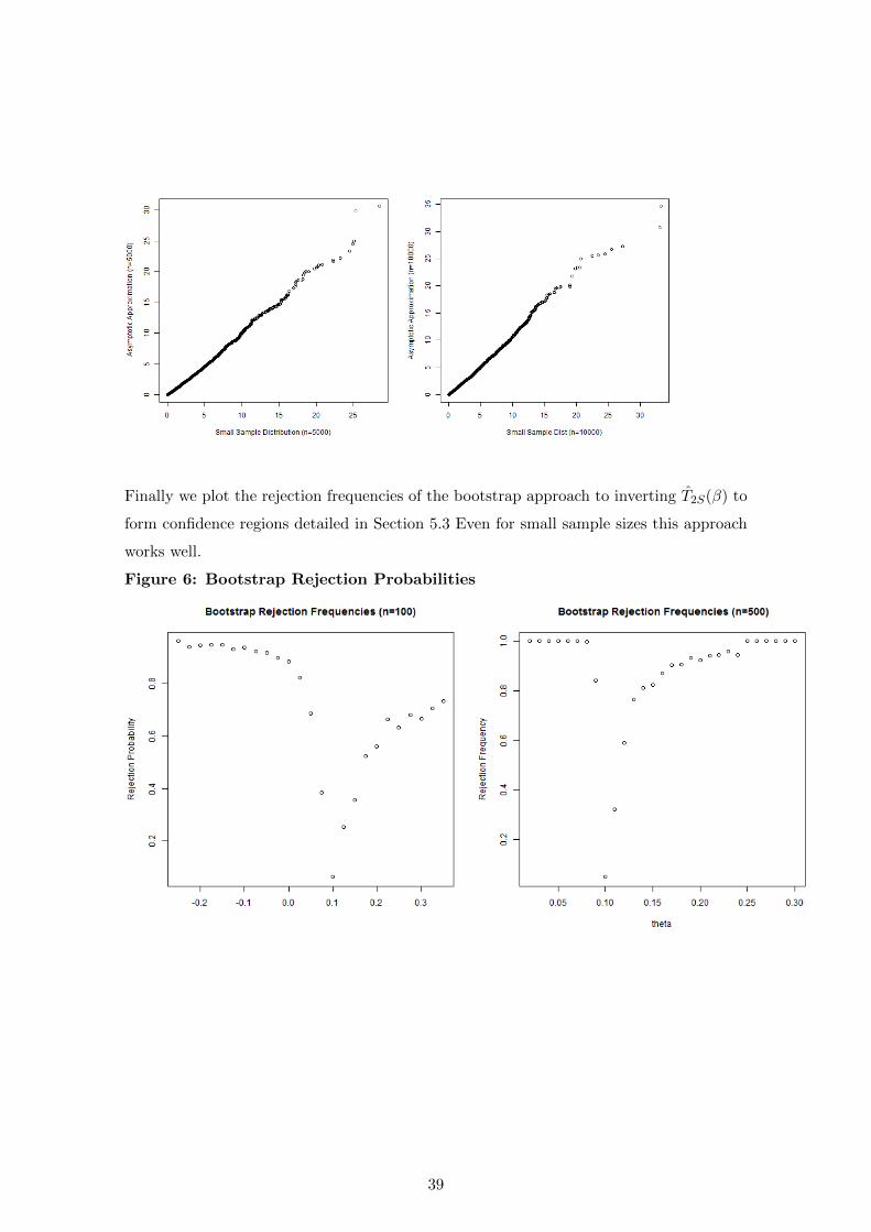
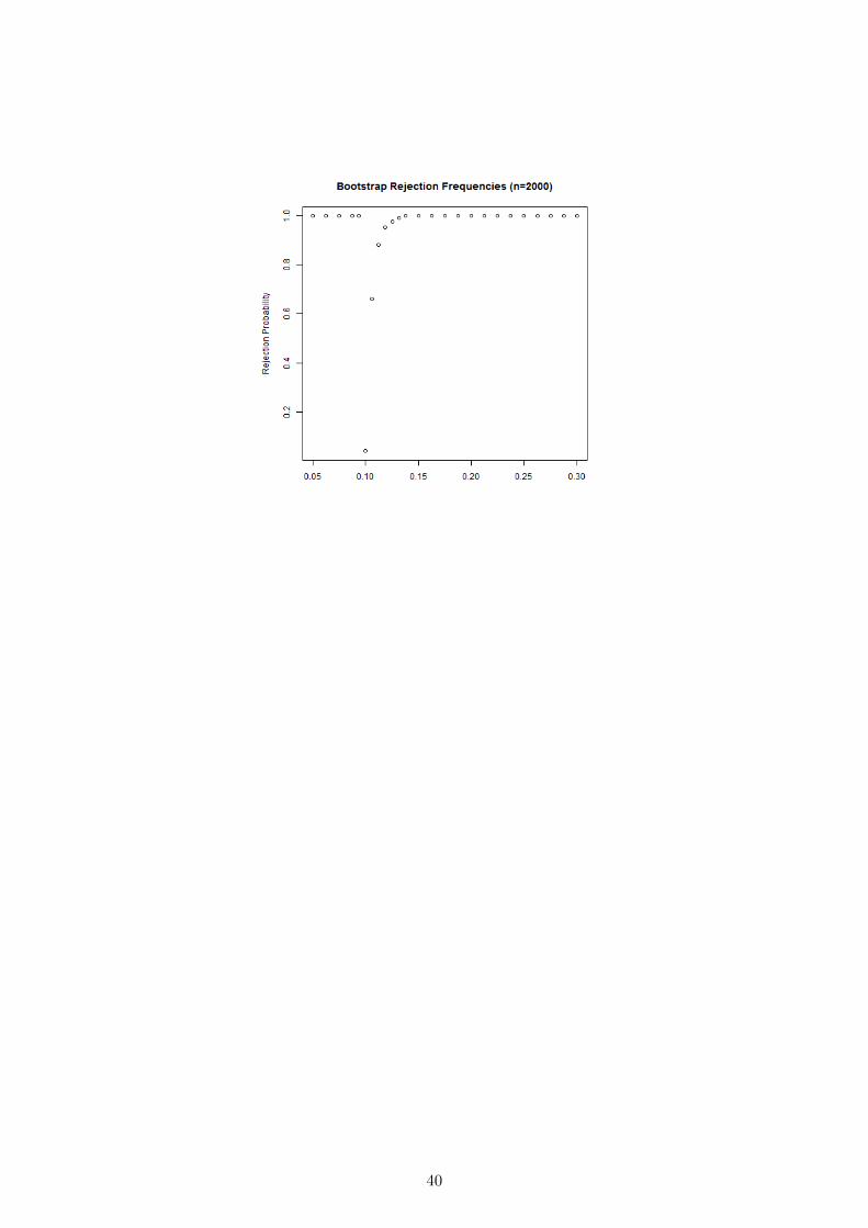
Finally we plot the rejection frequencies of the bootstrap approach to inverting T2S(β) to

form confidence regions detailed in Section 5.3 Even for small sample sizes this approach

works well.

Figure 6: Bootstrap Rejection Probabilities

39

40

6.3 Anderson Rubin

Since R(G) = 2 and R(Ω) = 1 when ρ = 1 then A2(iv) is not satisfied for the moment

set up in Simulation 1. Though it is beyond the scope of this paper to derive the limit

distribution of the AR statistic when A3 does not hold, this simulation shows how depar-

tures from A2 can lead to highly non standard limit distributions for the AR statistic.

We simulate 20000 times TAR(βn) for βn = β0 + 1/N for n = 100, 1000, 5000, 50000 for

p = 0.999999, 1

Figure 7: QQ-Plot of TAR(βn) and χ2m (p=1)

41

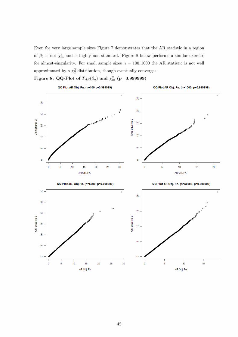
Even for very large sample sizes Figure 7 demonstrates that the AR statistic in a region

of β0 is not χ2m and is highly non-standard. Figure 8 below performs a similar exercise

for almost-singularity. For small sample sizes n = 100, 1000 the AR statistic is not well

approximated by a χ22 distribution, though eventually converges.

Figure 8: QQ-Plot of TAR(βn) and χ2m (p=0.999999)

42

6.4 Simulation 2: Parametric Semi-Linear Regression

Consider the following Semi-Linear model.

yi = π0xi + δ0 exp(γ0xi) + εi (68)

Where yi, xi are both scalar i.i.d variables where E[εi|xi] = 0. Define β = (π, δ, γ) ,

εi(β) = yi − πxi − δ exp(γxi)

Then ∂εi(β)/∂β = (xi, exp(γxi), δ exp(γxi)xi)′ and gi(β) = εi(β)(xi, exp(γxi), δ exp(γxi)xi)

′

Ω(β) = σ2E

x2i xi exp(γxi) δ exp(γxi)x

2i

xi exp(γxi) exp(2γxi) δ exp(2γxi)xi

δ exp(γxi)x2i exp(2γxi)xi δ2 exp(2γxi)x

2i

(69)

To test that the conditional mean is linear we test the parameter restriction that δ0 = 0.

In this case γ0 is globally under-identified. Tests of δ0 = 0 that overcome this problem are

given by Hansen (1996) and others.

When forming confidence sets for β0 when δ0 the variance of the moment function is also

singular. As such the sample variance estimated at β0 is also singular. As such many

identification robust statistics will not exist at the true parameter.

Another possibility is that γ0 = 0 (where δ0 6= 0). Then R(Ω) = 2 which also implies that

G = 2 by Theorem 1 and is easy to see by (). Since at γ0 = 0 ∂εi(β0)/∂β = (xi, 1, δxi)′.

Hence the third moment is a linear combination of the first. In this case the GMM

estimator is consistent, though the no longer has a standard limit distribution, Donovon

& Renault (2009).

We consider the following DGP

yi = exp(δxi) + xi + εi (70)

Where εiiid∼ N(0, 1), xi

d∼ U(0, 5) For δ = 0, 0.075, 0.1. When δ = 0 we have first order

under-identification and singular variance. For δ = 0.1 then thought Ω and G are full

rank, they have the smallest eigenvalue close to zero and hence are almost singular. Hence

standard asymptotic provide a poor approximation for both the GMM estimator and the

2-Step GMM objective function in small samples.

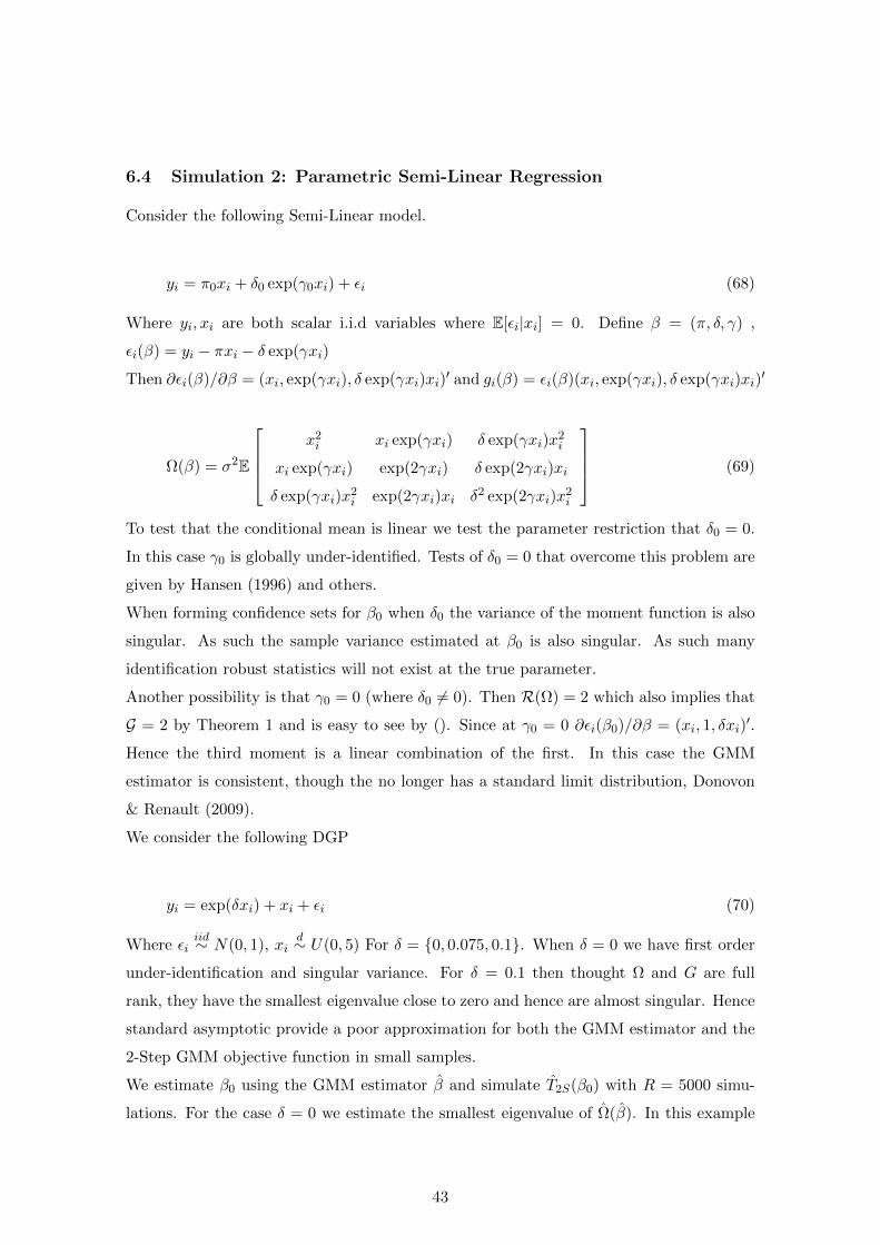
We estimate β0 using the GMM estimator β and simulate T2S(β0) with R = 5000 simu-

lations. For the case δ = 0 we estimate the smallest eigenvalue of Ω(β). In this example

43

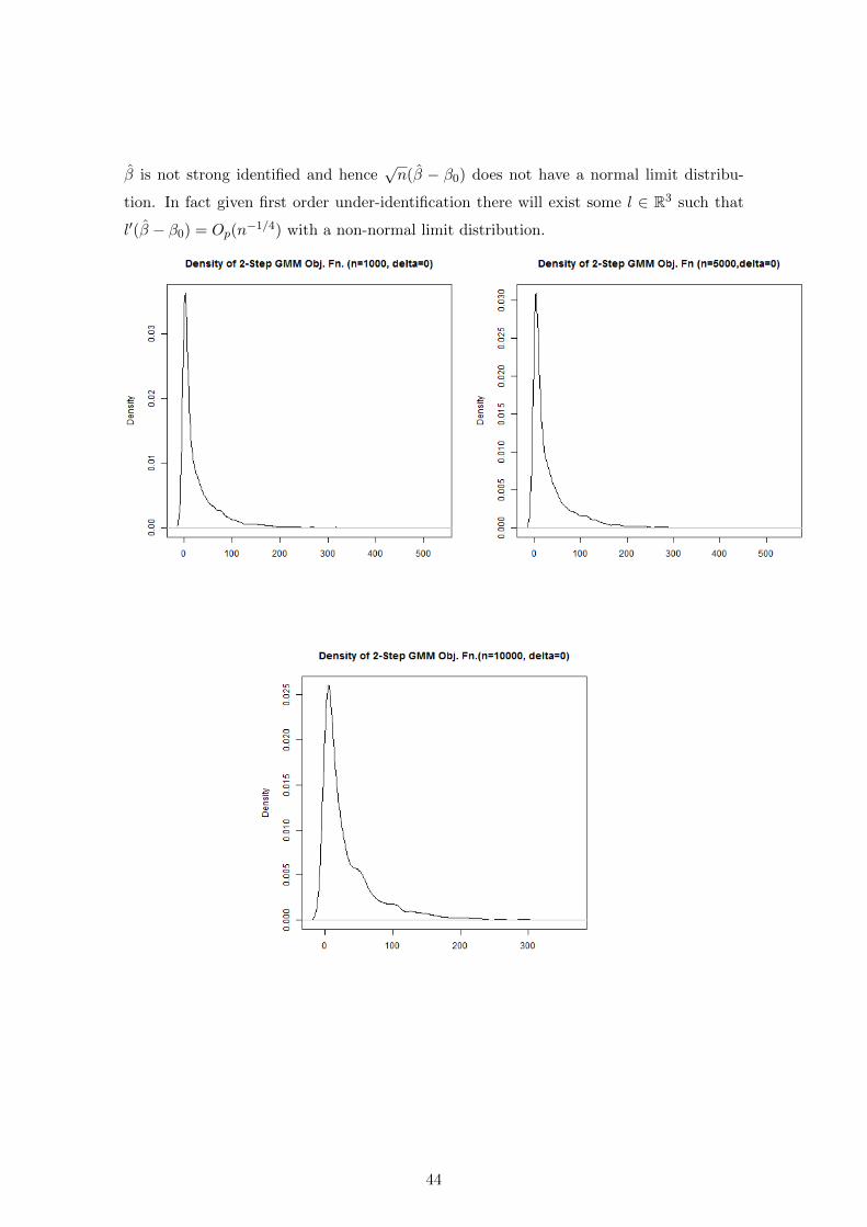
β is not strong identified and hence√n(β − β0) does not have a normal limit distribu-

tion. In fact given first order under-identification there will exist some l ∈ R3 such that

l′(β − β0) = Op(n−1/4) with a non-normal limit distribution.

44

45

46

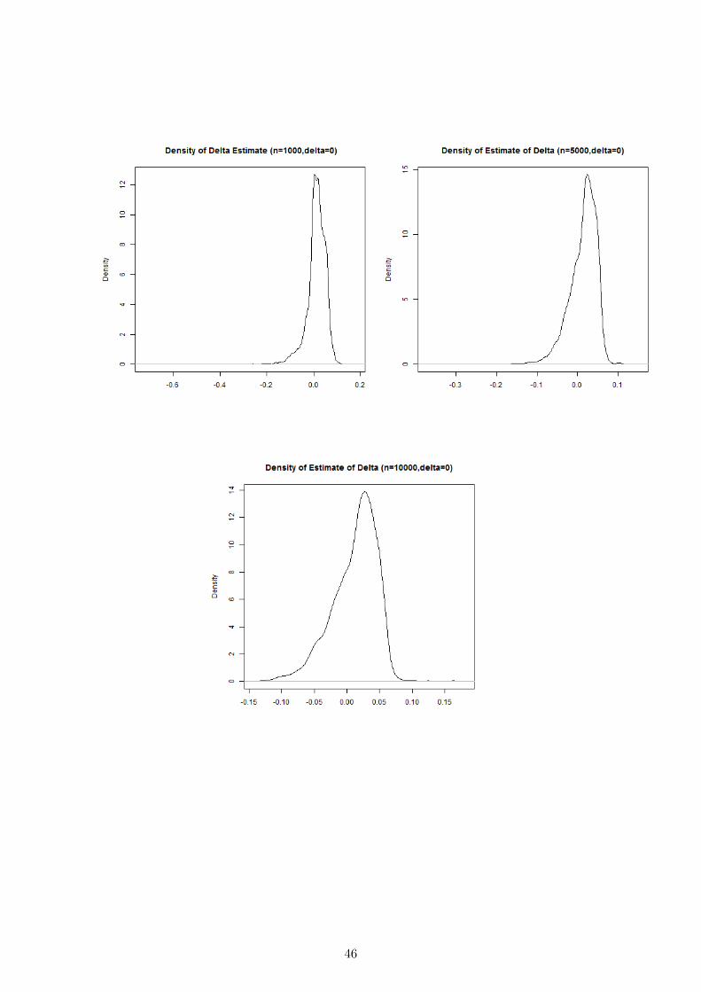
We now consider δ0 = 0.075, 0.1. In this case Ω and G are close to singular, as such we

expect strong identification asymptotic to provide a poor approximation to the distribution

of the GMM estimator and the 2-Step GMM objective function at β0.

47

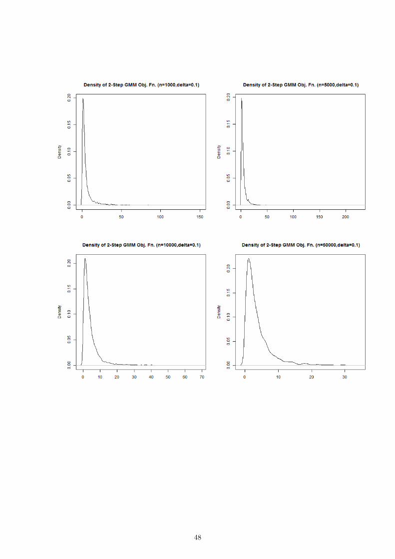
48

6.5 Anderson Rubin

We consider the AR statistic for Simulation 2 for βn = β0+1/N for n = 5000, 10000, 50000

based on 50000 repetitions.

49

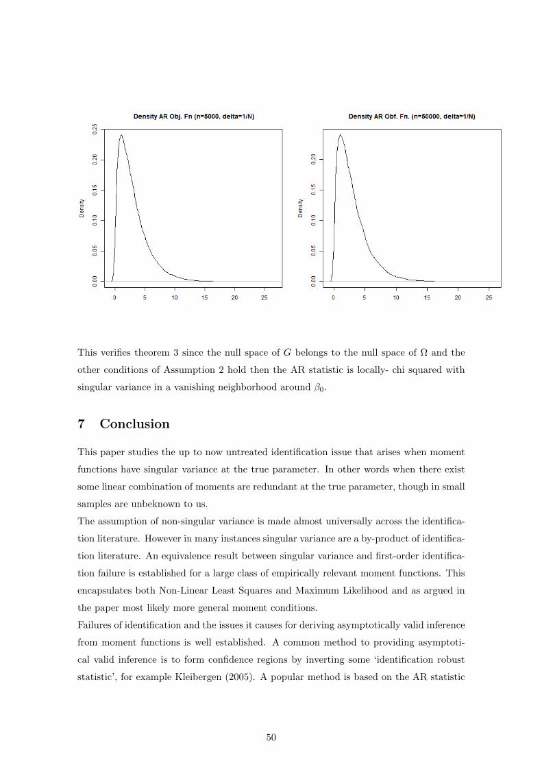
This verifies theorem 3 since the null space of G belongs to the null space of Ω and the

other conditions of Assumption 2 hold then the AR statistic is locally- chi squared with

singular variance in a vanishing neighborhood around β0.

7 Conclusion

This paper studies the up to now untreated identification issue that arises when moment

functions have singular variance at the true parameter. In other words when there exist

some linear combination of moments are redundant at the true parameter, though in small

samples are unbeknown to us.

The assumption of non-singular variance is made almost universally across the identifica-

tion literature. However in many instances singular variance are a by-product of identifica-

tion literature. An equivalence result between singular variance and first-order identifica-

tion failure is established for a large class of empirically relevant moment functions. This

encapsulates both Non-Linear Least Squares and Maximum Likelihood and as argued in

the paper most likely more general moment conditions.

Failures of identification and the issues it causes for deriving asymptotically valid inference

from moment functions is well established. A common method to providing asymptoti-

cal valid inference is to form confidence regions by inverting some ‘identification robust

statistic’, for example Kleibergen (2005). A popular method is based on the AR statistic

50

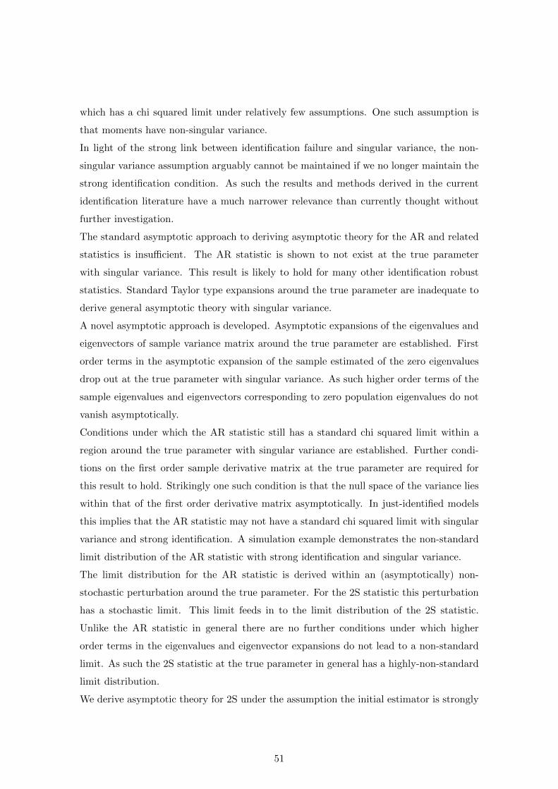
which has a chi squared limit under relatively few assumptions. One such assumption is

that moments have non-singular variance.

In light of the strong link between identification failure and singular variance, the non-

singular variance assumption arguably cannot be maintained if we no longer maintain the

strong identification condition. As such the results and methods derived in the current

identification literature have a much narrower relevance than currently thought without

further investigation.

The standard asymptotic approach to deriving asymptotic theory for the AR and related

statistics is insufficient. The AR statistic is shown to not exist at the true parameter

with singular variance. This result is likely to hold for many other identification robust

statistics. Standard Taylor type expansions around the true parameter are inadequate to

derive general asymptotic theory with singular variance.

A novel asymptotic approach is developed. Asymptotic expansions of the eigenvalues and

eigenvectors of sample variance matrix around the true parameter are established. First

order terms in the asymptotic expansion of the sample estimated of the zero eigenvalues

drop out at the true parameter with singular variance. As such higher order terms of the

sample eigenvalues and eigenvectors corresponding to zero population eigenvalues do not

vanish asymptotically.

Conditions under which the AR statistic still has a standard chi squared limit within a

region around the true parameter with singular variance are established. Further condi-

tions on the first order sample derivative matrix at the true parameter are required for

this result to hold. Strikingly one such condition is that the null space of the variance lies

within that of the first order derivative matrix asymptotically. In just-identified models

this implies that the AR statistic may not have a standard chi squared limit with singular

variance and strong identification. A simulation example demonstrates the non-standard

limit distribution of the AR statistic with strong identification and singular variance.

The limit distribution for the AR statistic is derived within an (asymptotically) non-

stochastic perturbation around the true parameter. For the 2S statistic this perturbation

has a stochastic limit. This limit feeds in to the limit distribution of the 2S statistic.

Unlike the AR statistic in general there are no further conditions under which higher

order terms in the eigenvalues and eigenvector expansions do not lead to a non-standard

limit. As such the 2S statistic at the true parameter in general has a highly-non-standard

limit distribution.

We derive asymptotic theory for 2S under the assumption the initial estimator is strongly

51

identified. Deriving the limit distribution with identification failures would in general prove

very difficult and is beyond the scope of this paper. A simulation experiment plots the

small sample distribution of the 2S statistic both with and without identification failure.

In both cases the standard chi squared critical values were largely undersized.

When the variance of the moments is non-singular though near to a point of singular-

ity simulation evidence shows that the chi squared approximation can be poor even for

extremely large sample sizes for the 2S statistic. This result is analogous to the normal

approximation to the distribution of the linear IV estimator being poor for large sample

sizes when there is weak identification. In this paper we derived asymptotic for the case

where the minimum eigenvalue of the population variance matrix is zero for finite n.

In light of the simulation evidence that the chi squared approximation to the small sample

distribution of the 2S statistic is poor even for large sample sizes, it would be valuable

to model the minimum eigenvalues as local-to zero. This approach is commonly used to

model weak identification, modeling the Jacobian as vanishing at some rate, Staiger &

Stock (1997), Newey & Windmeijer (2009). This is the approach taken in Grant (2012)

which is termed ‘Weak Singularity’.

In light of the problem that (almost) singular moments cause for inference we developed

a method of testing for redundant moments. The limit distribution of the minima of

the sample eigenvalue is established. With this we show how we can test the rank of

the population variance matrix at the true parameter. We also provided a method to

determine the rank of the matrix with probability one.

Using this approach we show how a modification to the 2S statistic eradicates the problem

of singular moments, yielding back a standard chi squared limit with an estimable degree

of freedom. We also detailed a bootstrap method which was shown to work well in two

simulations. Both with strong identification and underidentified with singular moments.

We term forming confidence sets utilizing such methods as ‘singularity robust confidence

sets’. We did not show theoretical validity of the bootstrap and is left for future research.

Numerous examples of singular variance both with and without identification failures are

provided. These issues are especially prevalent in non-linear models. As such these results

are especially useful for financial econometric models and discrete choice models.

A further investigation in to the more general link between identification failures and

singular variance is needed. Along with more general asymptotic theory which does not

maintain the assumption of singular variance. The question tackled in this paper poten-

tially opens up a large and empirically relevant question.

52

Given that singular variance and identification failures are closely linked; what is the

theoretical implication for commonly used estimation and inference results provided in

the econometric estimation literature? Which results remain the same in spite of singular

variance (and if so under which further conditions) and which do not? Which methods

overcome such problems if any of singular variance?

These questions cannot be underestimated in terms of their deep importance if one wishes

to confidently form valid inference from a set of moment conditions. This paper is the first

step in providing answers to these important questions and tools to study implications of

singular variance for other key inferential procedures.

8 Appendix

Definitions

For any random variables x E[x] refers to the mathematical expectation taken with respect

to (w.r.t) the density of x. Denotep→ ,

d→, as convergence in probability and convergence in

distribution respectively. For any deterministic sequence an and constant b then an → b

denotes b as the deterministic limit of an.d∼ is shorthand for ‘ is distributed as” and

‘w.p.a.1’ denotes ‘with probability approaching 1’ and ‘w.p.1’ denotes ‘with probability 1’.

op(a) refers to a variable that converges to zero w.p.a.1 when divided by a and similarly

Op(a) a variable bounded in probability when divided by a. Let A refer to any arbitrary

matrix then R(·) be such that R(A) N (A) denote the rank of A .||A|| and tr(A) are the

Euclidean Norm and Trace of a matrix A respectively. CMT refers to the Continuous

Mapping Theorem. For any a > 0 Ia×a refers to the a×a Identity Matrix and 0a an a× 1

vector of zeroes.

Lemma A Let A and A be two square matrices of dimension r whereA = r∗ and ||A−A|| =

Op(εn). Eigen-decompose A = RDR′ where RR′ = I and RDR′ = R1D1R′1 + R2D2R

′2

where D2 = 0 and D1 is a full rank (r − r∗) × (r − r∗) matrix. Similarly we express

A = RDR′ = R1D1R1 + R2D2R′2. Let M be some basis of the null space of A and define

B = (A−A) and J = −D−11 R′1BR2M where MM ′ = Im

R1 = R1 +R2MJ ′ +Op(ε2n) (71)

R2 = R2M +R1J +Op(ε2n) (72)

Where M is a change of basis such to validate asymptotic expansion in the more general

case when A is not square. For square matrices M = I. At any rate a change of basis

53

would not change any of the results as we could switch bases and work with R2 := R2M

and R2 := R2M . Hence () is equivalent to where implicitly we have shifted the basis of Ω

and Ω. Hence we can set M = Im and the results in this paper will not change.

R2 = R2 +R1J +Op(ε2n) (73)

Proof of Lemma A This general result is utilized in the proof of Proposition 1 of

Ratsimalahelo (2001). See equations A8 and A9 in the proof of Proposition 1.

Lemma B Under Assumption 1

P ′2jΩ(βn)P2j = γjn +Op(||∆3n||) (74)

Proof of Lemma B

Ω(βn) = 1n

∑ni=1 gi(βn)gi(βn)

Taylor expand gi(βn) around β0 where gi = gi(β0)

gi(βn) = gi +Gi(βn)∆n (75)

Where βn is a vector between β0 and βn Define Gi := Gi(βn)

Ω(βn) =1

n

n∑i=1

gig′i +

1

n

n∑i=1

Gi∆n∆′nG′i

+1

n

n∑i=1

gi∆′nG′i +

1

n

n∑i=1

Gi∆ng′i (76)

By Theorem 1 PrP ′2jgi(β0) = 0 = 1 and ∀i ∈ 1, .., n.

Hence 1n

∑ni=1(p′2jgi(β0))2 = 0 ∀ j ∈ 1, , m except on a set of measure zero for j =

1, .., m So that w.p.1

P ′2jΩ(βn)P2j =1

n

n∑i=1

P ′2jGi∆n∆′nG′iP2j (77)

Since by A1(iv) it is straightforward to establish that

|| 1n

n∑i=1

(GiGi −GtGi)|| = ||M ||||β∗n − β0|| = Op(||∆n||) (78)

And by construction||P2j ||2 = 1 then since by A1(v) || 1n∑n

i=1Gi(β0)|| = Op(1) it is straight-

forward to show that

1

n

n∑i=1

P ′2jGi∆n∆′nG′iP2j =

1

n

n∑i=1

P ′2jGi∆n∆′nG′iP2j +Op(||∆n||3) (79)

54

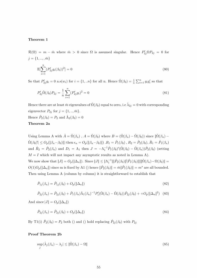
Theorem 1

R(Ω) = m − m where m > 0 since Ω is assumed singular. Hence P ′2jΩP2j = 0 for

j = 1, .., , m

E[

n∑i=1

(P ′2jgi(β0))2] = 0 (80)

So that P ′2jgi = 0 a.s(wi) for i = 1, ..n for all n. Hence Ω(β0) = 1n

∑ni=1 gig

′i so that

P ′2jΩ(β0)P2j =1

n

n∑i=1

(P ′2jgi)2 = 0 (81)

Hence there are at least m eigenvalues of Ω(β0) equal to zero, i.e λ2j = 0 with corresponding

eigenvector P2j for j = 1, .., m.

Hence P2(β0) = P2 and Λ2(β0) = 0

Theorem 2a

Using Lemma A with A = Ω(βn) , A = Ω(β0) where B = (Ω(βn)− Ω(β0)) since ||Ω(βn)−

Ω(β0|!| ≤ Op(||βn−β0)||) then εn = Op(||βn−β0)||) .R1 = P1(β0) , R2 = P2(β0), R1 = P1(βn)

and R2 = P2(βn) and D1 = Λ1 then J = −Λ−11 P1(β0)′(Ω(β0) − Ω(βn))P2(β0) (setting

M = I which will not impact any asymptotic results as noted in Lemma A).

We now show that ||J || = Op(||∆n||). Since ||J || ≤ ||Λ−11 ||||P2(β0)||||P1(β0)||||||Ω(βn)−Ω(β0)|| =

O(1)Op(||∆n||) since m is fixed by A1 () hence ||P2(β0)|| = m||P1(β0)|| = m∗ are all bounded.

Then using Lemma A (column by column) it is straightforward to establish that

P1j(βn) = P1j(β0) +Op(||∆n||) (82)

P2j(βn) = P2j(β0) + P1(βn)Λ1(βn)−1P ′1(Ω(βn)− Ω(β0))P2j(β0) + +Op(||∆n||2) (83)

And since |J || = Op(||∆n||)

P2j(βn) = P2j(β0) +Op(||∆n||) (84)

By T1(i) P2(β0) = P2 both () and () hold replacing P2j(β0) with P2j

Proof Theorem 2b

supj|λj(βn)− λj | ≤ ||Ω(βn)− Ω|| (85)

55

By an application Theorem 4.2 of Bosq (2000). By A1 (ii) (ii) and T then ||Ω(βn) −

Ω|| ≤ ||Ω(βn) − Ω(β0)|| + ||Ω(β0) − Ω|| = Op(||∆n||) + Op(n−1/2). This establishes that

λj = λj +Op(n−1/2 ∨ ||∆n||) for all j = 1, ..m and hence establishes (i). We not proceed

to prove (ii) which derives a second order expansion of λ2j)(βn) around β0 for j = 1, .., m

(ii)

nP ′2Ω(βn)P2 = nP ′2P1(βn)Λ1(βn)P1(βn)′P2 + P ′2P2(βn)Λ2(βn)P2(βn)′P2 (86)

By T2a(ii) P ′2P2(βn) = Im + Op(||∆n||2) and P1(βn) = Ω(βn)P1(βn)Λ1(βn)−1 where by

Theorem 1a (i) ||P1(βn)−P1|| = Op(n−1/2 ∨ ||∆n|| and T2b(i) ||Λ1(βn)−Λ1|| ≤ Op(n−1/2 ∨

||∆n||) and P ′2Ω(βn) = P ′2(Ω(βn)− Ω(β0) where ||Ω(βn)− β0|| = Op(||∆n||) and ||P2|| = m =

O(1) by A1 and Λ2(βn) ≤ Op(n−1/2 ∨ ||∆n) by () then straightforward manipulation will

demonstrate that

P ′2Ω(βn)P2 = Λ2(βn) + P ′2Ω(βn)P1Λ−11 P ′1Ω(βn)P2 +Op(∆n||2(∆n ∨ n−1/2) (87)

Hence for all j = 1, ..,m

λ2j(βn) = P ′2jΩ(βn)P2j − P ′2jΩ(βn)P1Λ−11 P ′1Ω(βn)P2j −Op(∆n||2(∆n ∨ n−1/2) (88)

By T1 and ()

P ′2jΩ(βn)P1 = P ′2j1

n

n∑i=1

Gi∆ng′iP1 +

1

n

n∑i=1

P ′2jGi∆n∆nG′iP1 (89)

A1( iv), (v) it is straightforward to establish (similar to the proof of Lemma B) tat

P ′2jΩ(βn)P1 = P ′2j1

n

n∑i=1

Gi∆ng′iP1 +Op(||∆n||2) (90)

P ′2jΩ(βn)P1Λ−11 P ′1Ω(βn)P2j =

+P ′2j1

n

n∑i=1

Gi∆ng′iP1

1

nΛ−1

1

n∑j=1

P ′1gi∆′nGiP2j +Op(||∆n||3) (91)

and Lemma B by A1

λ2j(βn) = γjn − ψjn +Op(||∆n||2(||∆n|| ∨ n−1/2) (92)

Proof of Theorem 3

TAR(βn) =√ng(βn)′Ω(βn)−1√ng(βn)

56

=m∗∑j=1

(P1j(βn)′√ng(βn))2λ−1

1j +m∑j=1

(P2j(βn)′√ng(βn))2λ2j(βn)−1 (93)

Firstly second order expand g(βn) around β0

g(βn) = g(β0) + G(β0)∆n +Op(n−2κ) (94)

By A1 (i),(iii). Then by Theorem 2a (i)P1j(βn) = P1j + Op(n−1/2 since ||∆n|| = Op(n

−κ)

by A2(i) where κ > 1/2 and similarly by Theorem 2b (i) λ1j(βn) = λ1j + Op(n−1/2)

∀j = 1, ..,m∗ By () and ()

(P1j(βn)′√ng(βn))2/λ1j = (P ′1j

√ng(β0))2/λ1j +Op(n

1/2−κ) (95)

Then by A2(iii) n1/2g(β0)d→ N(0,Ω) hence P ′1j

√ng(β0)/λ1j

d→ N(0, 1)

m∗∑j=1

(P1j(βn)′√ng(βn))2/λ1j

d→ χ2m∗ (96)

The case where m = m∗ we have the standard result that AR is χ2m

By Theorem 2(b)and

n2κλ2j(βn)p→ γjn − ψjn +Op(||∆n||2(n−1/2 ∨ ||∆n||) (97)

And by A2(iv) n2κ(γjn − ψjn)p→ γj − ψj = υj so that

n2κλ2j(βn)p→ υj (98)

nκP2j(βn)′√ng(βn) (99)

By Theorem 2b (ii)

P2j(βn) = P2j + P1Λ−11 P ′1Ω(βn)P2j +Op(||∆n||(n−1/2 ∨ ||∆n||) (100)

And using ()

nκ+1/2g(βn) = nκ+1/2g(β0) +√nG(β0)nκ∆n +Op(n

1/2−κ) (101)

Where by A1(i) κ > 1/2

Hence substituting () into () in to ()

(nκP2j(βn)′√ng(βn)) =

57

P ′2j√nG(β0)nκ∆n − nκ(P ′2jΩ(βn)P1Λ−1

1 P ′1√ng(β0) + op(1) (102)

A1(i)nκ∆′n→p∆

nκP ′2jΩ(βn)P1Λ−1/21 = P ′2j

1

n

n∑i=1

Ginκ∆ng

′iP1Λ

−1/21 +Op(n

−κ) (103)

P ′2j1

n

n∑i=1

Ginκ∆ng

′iP1Λ

−1/21

p→ 1

n

n∑i=1

P ′2jE[Gi∆g′i]P1Λ

−1/21 = Ψj (104)

By A2() ||√ng(β0)|| = Op(1) so that

(nκP2j(βn)′√ng(βn)) = P ′2j

√nG(β0)∆−ΨjΛ

−1/21 P ′1

√ng(β0) + op(1) (105)

Λ−1/21 P ′1

√ng(β0)

d→ N(0, Im∗) (106)

ΨjΛ−1/21 P ′1

√ng(β0)

d→ N(0, ψj) (107)

By A2 (iii) P ′2jG = 0 for all j = 1, .., m

G(β0)′P2j = (G(β0)−G)′P2jd→ N(0,Φj) (108)

Where Φj := E[ 1nG′iP2jP2jGi]. Since by then by Slutksys Theorem and ()

∆′G(β0)′P2jd→ N(0,∆′Φj∆) (109)

∆′Ψj∆ = tr(∆′E[1

nG′iP2jP

′2jGi]∆) = P ′2jE[

1

n

n∑i=1

G′i∆∆′Gi]P2j = γj (110)

Since

P ′2j√nG(β0)∆(P1Λ−1

1 P ′1Φj

√ng(β0))′

p→ ψj (111)

Then

nκP2j(βn)′√ng(βn)

d→ N(0, γj − ψj) (112)

Then by Theorem 1b(ii) and A3() n2κλj(βn)p→ υj

m∑j=1

(nκP2j(βn)′√ng(βn)/λj(βn)1/2)2 d→ χ2

m (113)

58

Theorem 4 Since ∆n = β − β0 for 2S-GMM By A3(1) ||∆n|| = Op(n−1/2) so that by

T2b(i)

λ2j(β) = υjn +Op(n−3/2) (114)

Where υjn = P ′2j1n

∑ni=1G

′i∆n∆′nGi − 1

n

∑nl=1(Gi∆n∆′nGl)(g

′iP1Λ−1

1 P ′1gl)P2j

nλ2j(β) = ntr(υjn) +Op(n−1/2)

= tr(P ′2j1

n

n∑i=1

G′in∆n∆′nGi −1

n

n∑l=1

Gin∆n∆′nGl(g′iP1Λ−1

1 P ′1gl)P2j) +Op(n−1/2)

= tr(1

n

n∑i=1

G′iP2jP′2jGi−

1

n

n∑l=1

GiP2jP′2jGl(g

′iP1Λ−1

1 P ′1gl)n∆n∆′n)+Op(n−1/2) (115)

By A3(ii) then

Υ′

(1

n

n∑i=1

G′iP2jP′2jGi −

1

n

n∑l=1

GiP2jP′2jGl(g

′iP1Λ−1

1 P ′1gl)

)Υ := Πjn

p→ Πj (116)

Since ∆n = β − β0 by A3(i) and A2(ii)

n1/2∆nd→ ΣN(0,Ω)

d= ΣP1Λ

1/21 Z (117)

Where Zd∼ N(0, Im∗) and Υ := ΣP1Λ

1/21

nλ2j(β)d→ tr(ΠjZZ

′) (118)

Where ZZ ′ is a m∗ ×m∗ matrix with a standard Wishart distribution.

Theorem 5

T2S(β0) = ng(β0)′Ω(β)−1g(β0)

=

m∗∑j=1

(P1j(β)′√ng(β0))2λ1j(β)−1 +

m∑j=1

(P2j(β)′√ng(β0))2λ2j(β)−1 (119)

Define Zh as the standard normal variable such that n1/2P1hλ−1/21h

d→ Zh for h = 1, ..m∗

where Zi and Zj are independent ∀i 6= j.

Since by A3 (ii) β − β0 = Op(n−1/2) then using T2 P1j(β)

p→ P1j and λ1j(β)p→ λ1j then

by a similar arguments to the proof of T3 equation (92)

m∗∑j=1

(P1j(β)′√ng(β0))2λ1j(β)−1 d→

m∗∑h=1

Z2h (120)

59

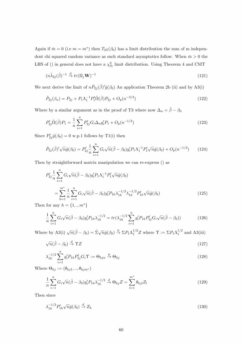
Again if m = 0 (i.e m = m∗) then T2S(β0) has a limit distribution the sum of m indepen-

dent chi squared random variance as such standard asymptotics follow. When m > 0 the

LHS of () in general does not have a χ2m limit distribution. Using Theorem 4 and CMT

(nλ2j(β)−1 d→ tr(ΠjW)−1 (121)

We next derive the limit of nP2j(β)′g(β0) An application Theorem 2b (ii) and by A3(i)

P2j(βn) = P2j + P1Λ−11 P ′1Ω(β)P2j +Op(n

−3/2) (122)

Where by a similar argument as in the proof of T3 where now ∆n = β − β0

P ′2jΩ(β)P1 =1

n

n∑i=1

P ′2jGi∆ng′iP1 +Op(n

−1/2) (123)

Since P ′2j g(β0) = 0 w.p.1 follows by T1(i) then

P2j(β)′√ng(β0) = P ′2j

1

n

n∑i=1

Gi√n(β − β0)g′iP1Λ−1

1 P ′1√ng(β0) +Op(n

−1/2) (124)

Then by straightforward matrix manipulation we can re-express () as

P ′2j1

n

n∑i=1

Gi√n(β − β0)g′iP1Λ−1

1 P ′1√ng(β0)

=m∗∑h=1

1

n

n∑i=1

Gi√n(β − β0)g′iP1hλ

−1/21h λ

−1/21h P ′1h

√ng(β0) (125)

Then for any h = 1, .,m∗

1

n

n∑i=1

Gi√n(β − β0)g′iP1hλ

−1/21h = tr(λ

−1/21h

n∑i=1

g′iP1hP′2jGi√n(β − β0)) (126)

Where by A3(i)√n(β − β0) = Σ

√ng(β0)

p→ ΣP1Λ1/21 Z where Υ := ΣP1Λ

1/21 and A3(iii)

√n(β − β0)

d→ ΥZ (127)

λ−1/21h

n∑i=1

g′iP1hP′2jGiΥ := Θhjn

p→ Θhj (128)

Where Θhj := (θhj1, .., θhjm∗)

1

n

n∑i=1

Gi√n(β − β0)g′iP1hλ

−1/21h

d→ ΘhjZ =

m∗∑l=1

θhjlZl (129)

Then since

λ−1/21h P ′1h

√ng(β0)

d→ Zh (130)

60

So that by () and () which hold for all j = 1, ..m and h = 1, ..m∗

m∗∑h=1

1

n

n∑i=1

Gi√n(β − β0)g′iP1hλ

−1/21h λ

−1/21h P ′1h

√ng(β0)

d→m∗∑h=1

m∗∑l=1

θhjlZlZh (131)

So that by the CMT

(nP2j(β)′g(β0))2/(nλ2j(β))d→ (

m∗∑h=1

m∗∑l=1

θhjlZlZh)2/tr(ΠjZZ′) (132)

Then substituting () in to () and by () and define

T2S(β0)d→

m∗∑k=1

Z2k +

m∑j=1

(

m∗∑h=1

m∗∑l=1

θhjlZlZh)2/tr(ΠjZZ′) (133)

61

References

[1] Andrews, K. (19987). Asymptotic Results for Generalized Wald Tests, Econometric

Theory, Cambridge University Press, vol. 3(03), pages 348-358, June.

[2] Bathia, N. , Yao, Q. and Ziegelmann, F. (2010). Identifying the finite dimen-

sionality of curve time series, Ann. Statist. Volume 38, Number 6 (2010), 3352-3386.

[3] Bosq, D. (2000). Linear Processes in Function Spaces, New York: Springer- Verlag.

[4] Grant, N. (2012). GMM with Weakly Singular Variance (work in progress).

[5] Hansen, H.L (1982). Large Sample Properties of Generalized Method of Moments

Estimators, Econometrica, 50, issue 4, p. 1029-54

[6] Jagannathan, R. and Wang, G. (2002). Generalized Method of Moments: Appli-

cations in Finance, Journal of Business & Economic Statistics, American Statistical

Association, vol. 20(4), pages 470-81, October.

[7] Kato, T. (1982). A short introduction to the perturbation theory of linear operators.,

Springer-Verlag 1982.

[8] Kleibergen, F. (2005). Testing Parameters in GMM Without Assuming that They

Are Identified, Econometrica, Econometric Society, vol. 73(4), pages 1103-1123, 07.

[9] Kleibergen, F. (2011). Improved accuracy of weak instrument robust GMM statistics

through bootstrap and Edgeworth approximations, working paper.

[10] Newey, W. and McFadden,D. (1994). Large Sample Estimation and Hypothesis

Testing,Handbook of Econometrics, Vol.4, 2111-2245.

[11] Newey, W.N. and Windmeijer, F. (2009). Generalized Method of Moments With

Many Weak Moment Conditions, Econometrica, Econometric Society, vol. 77(3), pages

687-719, 05.

[12] Penaranda, F. and Sentana, E. (2010). Spanning tests in return and stochastic

discount factor mean-variance frontiers: A unifying approach, Economics Working Pa-

pers 1101, Department of Economics and Business, Universitat Pompeu Fabra, revised

Sep 2010.

62

[13] Renault, E. and Donovon, P. (2009). GMM Overidentification Test with First

Order Underidentification, working paper (2009).

[14] Sargan, J. D. (1983). Identification and Lack of Identification, Econometrica,

Econometric Society, vol. 51(6), pages 1605-33, November

[15] Staiger, D. and Stock, J.H. (1997). Instrumental Variables Regression with Weak

Instruments, Econometrica, Econometric Society, vol. 65(3):557-586.

[16] Stock, J.H. and Wright, J. (2000). GMM with Weak Identification,Econometrica,

Econometric Society, vol. 68(5), pages 1055-1096, September.

63