ICLEAC CONTRACT N : G4RD-CT2000-0215 PROJECT N · PDF fileInstability Control of Low Emission Aero-engine Combustors ... In a previous study, ... the mathematical models and dynamic

ICLEACInstability Control of Low Emission Aero-engine Combustors

CONTRACT N◦: G4RD-CT2000-0215

PROJECT N◦: GRD1-1999-10514

DELIVERABLE NUMBER: D4.8

TITLE: Rumble Prediction with Integrated CFD/Low-Model Method

M. Zhu, A. P. Dowling and K.N.C. Bray

Date of issue of this report: 01/03/2004

Project funded by the European Communityunder the ‘Competitive and SustainableGrowth’ Programme (1998–2002)

2

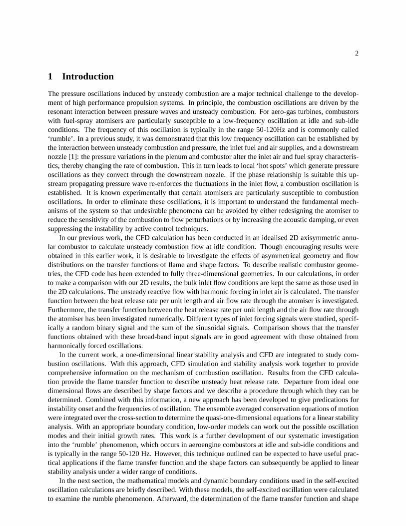
1 Introduction

The pressure oscillations induced by unsteady combustion are a major technical challenge to the develop-ment of high performance propulsion systems. In principle, the combustion oscillations are driven by theresonant interaction between pressure waves and unsteady combustion. For aero-gas turbines, combustorswith fuel-spray atomisers are particularly susceptible to a low-frequency oscillation at idle and sub-idleconditions. The frequency of this oscillation is typically in the range 50-120Hz and is commonly called‘rumble’. In a previous study, it was demonstrated that this low frequency oscillation can be established bythe interaction between unsteady combustion and pressure, the inlet fuel and air supplies, and a downstreamnozzle [1]: the pressure variations in the plenum and combustor alter the inlet air and fuel spray characteris-tics, thereby changing the rate of combustion. This in turn leads to local ‘hot spots’ which generate pressureoscillations as they convect through the downstream nozzle. If the phase relationship is suitable this up-stream propagating pressure wave re-enforces the fluctuations in the inlet flow, a combustion oscillation isestablished. It is known experimentally that certain atomisers are particularly susceptible to combustionoscillations. In order to eliminate these oscillations, it is important to understand the fundamental mech-anisms of the system so that undesirable phenomena can be avoided by either redesigning the atomiser toreduce the sensitivity of the combustion to flow perturbations or by increasing the acoustic damping, or evensuppressing the instability by active control techniques.

In our previous work, the CFD calculation has been conducted in an idealised 2D axisymmetric annu-lar combustor to calculate unsteady combustion flow at idle condition. Though encouraging results wereobtained in this earlier work, it is desirable to investigate the effects of asymmetrical geometry and flowdistributions on the transfer functions of flame and shape factors. To describe realistic combustor geome-tries, the CFD code has been extended to fully three-dimensional geometries. In our calculations, in orderto make a comparison with our 2D results, the bulk inlet flow conditions are kept the same as those used inthe 2D calculations. The unsteady reactive flow with harmonic forcing in inlet air is calculated. The transferfunction between the heat release rate per unit length and air flow rate through the atomiser is investigated.Furthermore, the transfer function between the heat release rate per unit length and the air flow rate throughthe atomiser has been investigated numerically. Different types of inlet forcing signals were studied, specif-ically a random binary signal and the sum of the sinusoidal signals. Comparison shows that the transferfunctions obtained with these broad-band input signals are in good agreement with those obtained fromharmonically forced oscillations.

In the current work, a one-dimensional linear stability analysis and CFD are integrated to study com-bustion oscillations. With this approach, CFD simulation and stability analysis work together to providecomprehensive information on the mechanism of combustion oscillation. Results from the CFD calcula-tion provide the flame transfer function to describe unsteady heat release rate. Departure from ideal onedimensional flows are described by shape factors and we describe a procedure through which they can bedetermined. Combined with this information, a new approach has been developed to give predications forinstability onset and the frequencies of oscillation. The ensemble averaged conservation equations of motionwere integrated over the cross-section to determine the quasi-one-dimensional equations for a linear stabilityanalysis. With an appropriate boundary condition, low-order models can work out the possible oscillationmodes and their initial growth rates. This work is a further development of our systematic investigationinto the ‘rumble’ phenomenon, which occurs in aeroengine combustors at idle and sub-idle conditions andis typically in the range 50-120 Hz. However, this technique outlined can be expected to have useful prac-tical applications if the flame transfer function and the shape factors can subsequently be applied to linearstability analysis under a wider range of conditions.

In the next section, the mathematical models and dynamic boundary conditions used in the self-excitedoscillation calculations are briefly described. With these models, the self-excited oscillation were calculatedto examine the rumble phenomenon. Afterward, the determination of the flame transfer function and shape

3

factors from a single forced CFD calculation are briefly introduced. With the air supply was modulated byforcing signal, which containing information at a range of frequencies pulse noise, the response of down-stream flow was recorded to calculate the flame transfer function. The method gives reliable information ofthe combustion response across a wide frequency band-width, and can be used in the low-order analysis inbelow. In section 3, the area-averaged equations for a quasi-one-dimensional stability analysis are derivedthrough integrating the equations of motion. Three non-dimensional shape factors are defined to account theeffects of non-uniformity in the radial direction. Based on the integrated equations, the equations for meanflow and linear perturbations are derived from these area-averaged equations. We integrate the models fromthis CFD calculation with the linear perturbation equations. The results are compared with those from CFDself-exciting calculation performed with the same inlet boundary conditions. The sensitivities of the shapefactor perturbations are also investigated. Finally, the conclusions are presented in section 4.

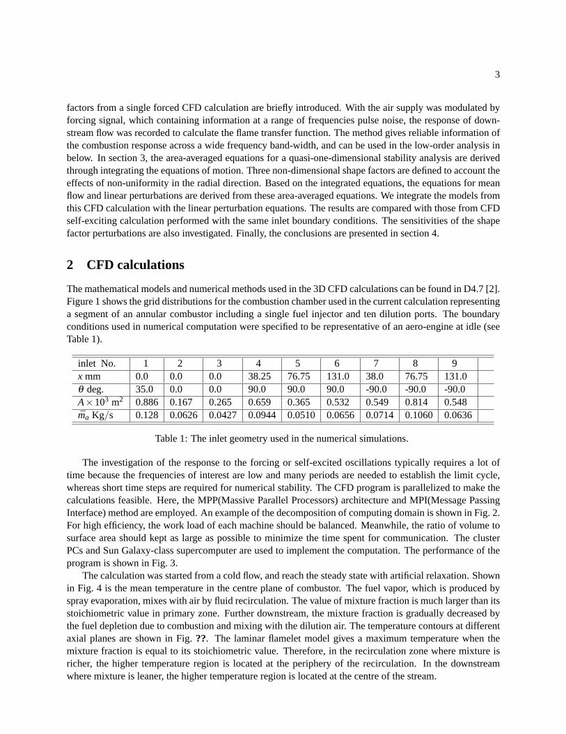
2 CFD calculations

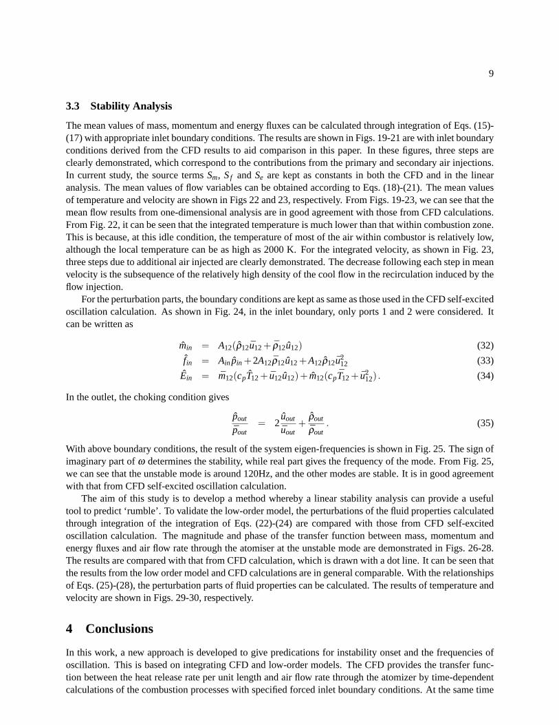
The mathematical models and numerical methods used in the 3D CFD calculations can be found in D4.7 [2].Figure 1 shows the grid distributions for the combustion chamber used in the current calculation representinga segment of an annular combustor including a single fuel injector and ten dilution ports. The boundaryconditions used in numerical computation were specified to be representative of an aero-engine at idle (seeTable 1).

inlet No. 1 2 3 4 5 6 7 8 9x mm 0.0 0.0 0.0 38.25 76.75 131.0 38.0 76.75 131.0θ deg. 35.0 0.0 0.0 90.0 90.0 90.0 -90.0 -90.0 -90.0A×103 m2 0.886 0.167 0.265 0.659 0.365 0.532 0.549 0.814 0.548ma Kg/s 0.128 0.0626 0.0427 0.0944 0.0510 0.0656 0.0714 0.1060 0.0636

Table 1: The inlet geometry used in the numerical simulations.

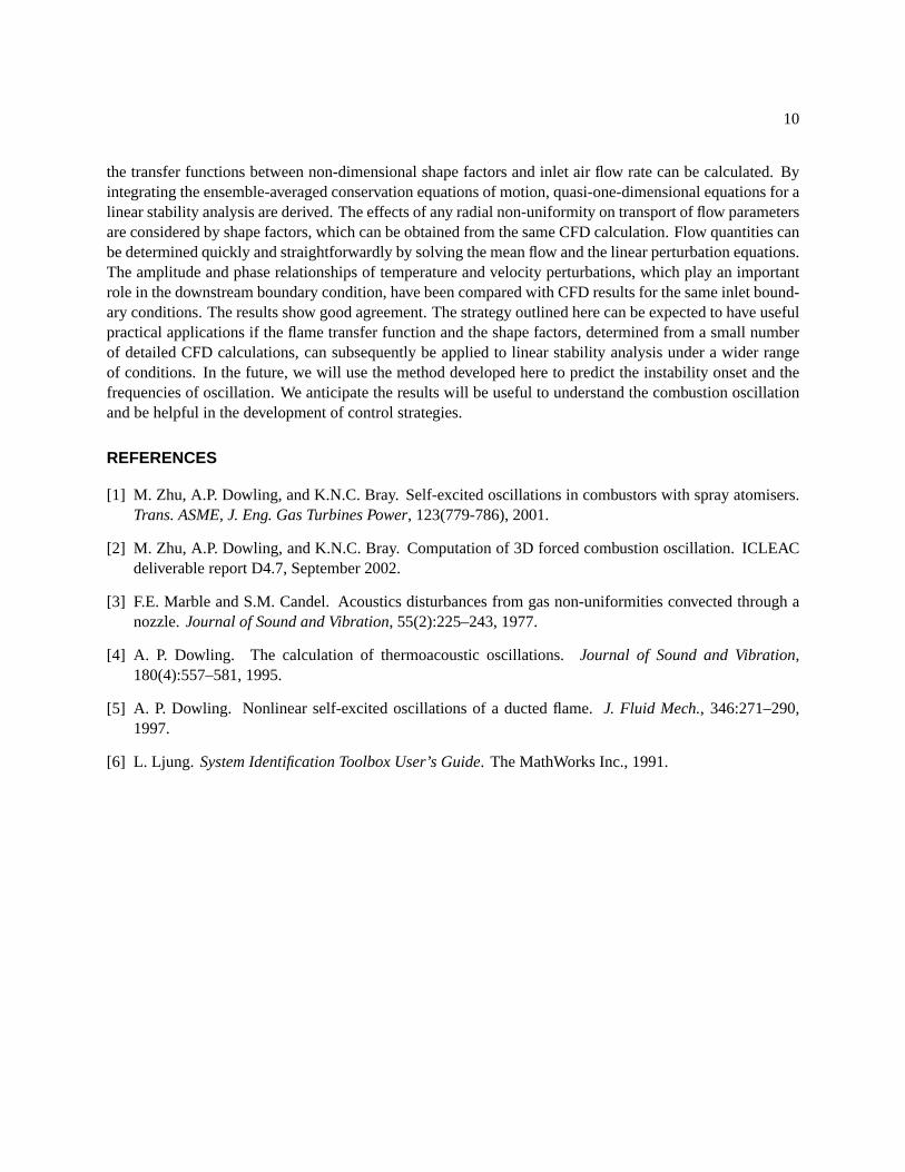
The investigation of the response to the forcing or self-excited oscillations typically requires a lot oftime because the frequencies of interest are low and many periods are needed to establish the limit cycle,whereas short time steps are required for numerical stability. The CFD program is parallelized to make thecalculations feasible. Here, the MPP(Massive Parallel Processors) architecture and MPI(Message PassingInterface) method are employed. An example of the decomposition of computing domain is shown in Fig. 2.For high efficiency, the work load of each machine should be balanced. Meanwhile, the ratio of volume tosurface area should kept as large as possible to minimize the time spent for communication. The clusterPCs and Sun Galaxy-class supercomputer are used to implement the computation. The performance of theprogram is shown in Fig. 3.

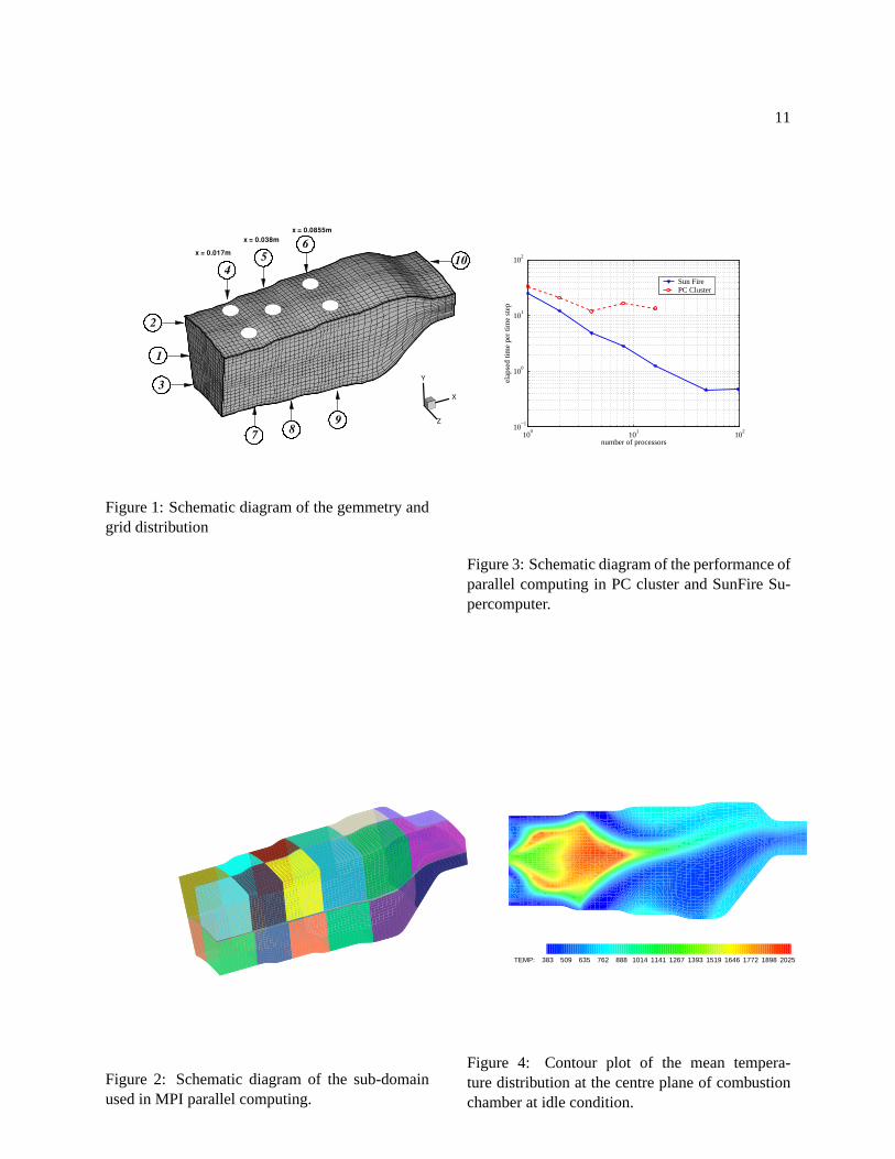
The calculation was started from a cold flow, and reach the steady state with artificial relaxation. Shownin Fig. 4 is the mean temperature in the centre plane of combustor. The fuel vapor, which is produced byspray evaporation, mixes with air by fluid recirculation. The value of mixture fraction is much larger than itsstoichiometric value in primary zone. Further downstream, the mixture fraction is gradually decreased bythe fuel depletion due to combustion and mixing with the dilution air. The temperature contours at differentaxial planes are shown in Fig.??. The laminar flamelet model gives a maximum temperature when themixture fraction is equal to its stoichiometric value. Therefore, in the recirculation zone where mixture isricher, the higher temperature region is located at the periphery of the recirculation. In the downstreamwhere mixture is leaner, the higher temperature region is located at the centre of the stream.

4

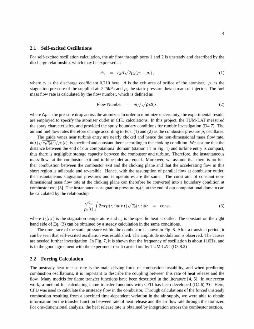
2.1 Self-excited Oscillations

For self-excited oscillation calculation, the air flow through ports 1 and 2 is unsteady and described by thedischarge relationship, which may be expressed as

ma = cdA√

2ρa(p0− ps) , (1)

wherecd is the discharge coefficient 0.710 here.A is the exit area of orifice of the atomiser.p0 is thestagnation pressure of the supplied air 225kPa andps the static pressure downstream of injector. The fuelmass flow rate is calculated by the flow number, which is defined as

Flow Number = mf /√

ρ f ∆p, (2)

where∆p is the pressure drop across the atomizer. In order to minimize uncertainty, the experimental resultsare employed to specify the atomiser outlet in CFD calculations. In this project, the TUM-LAT measuredthe spray characteristics, and provided the spray boundary conditions for rumble investigation (D4.7). Theair and fuel flow rates therefore change according to Eqs. (1) and (2) as the combustor pressureps oscillates.

The guide vanes near turbine entry are nearly choked and hence the non-dimensional mass flow rate,m(t)

√cpT0(t)/p0(t), is specified and constant there according to the choking condition. We assume that the

distance between the end of our computational domain (station 11 in Fig. 1) and turbine entry is compact,thus there is negligible storage capacity between the combustor and turbine. Therefore, the instantaneousmass flows at the combustor exit and turbine inlet are equal. Moreover, we assume that there is no fur-ther combustion between the combustor exit and the choking plane and that the accelerating flow in thisshort region is adiabatic and reversible. Hence, with the assumption of parallel flow at combustor outlet,the instantaneous stagnation pressures and temperatures are the same. The constraint of constant non-dimensional mass flow rate at the choking plane can therefore be converted into a boundary condition atcombustor exit [3]. The instantaneous stagnation pressurep0(t) at the end of our computational domain canbe calculated by the relationship

√cp

p0(t)

∫2πrρ(r, t)u(r, t)

√T0(r, t)dr = const. (3)

whereT0(r, t) is the stagnation temperature andcp is the specific heat at outlet. The constant on the righthand side of Eq. (3) can be obtained by a steady calculation in the same conditions.

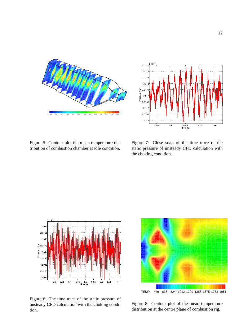
The time trace of the static pressure within the combustor is shown in Fig. 6. After a transient period, itcan be seen that self-excited oscillation was established. The amplitude modulation is observed. The causesare needed further investigation. In Fig. 7, it is shown that the frequency of oscillation is about 110Hz, andis in the good agreement with the experiment result carried out by TUM-LAT (D3.8.2)

2.2 Forcing Calculation

The unsteady heat release rate is the main driving force of combustion instability, and when predictingcombustion oscillations, it is important to describe the coupling between this rate of heat release and theflow. Many models for flame transfer functions have been described in the literature [4, 5]. In our recentwork, a method for calculating flame transfer functions with CFD has been developed (D4.6)??. Here,CFD was used to calculate the unsteady flow in the combustor. Through calculations of the forced unsteadycombustion resulting from a specified time-dependent variation in the air supply, we were able to obtaininformation on the transfer function between rate of heat release and the air flow rate through the atomizer.For one-dimensional analysis, the heat release rate is obtained by integration across the combustor section.

5

The ARX model is used in the transfer function calculation [6]. This means the transfer function at axialpositionx is written in the form of an IIR filter, with additional noise, i.e.

〈q〉(x,nT) =I−1

∑i=0

ai(x)ma[x,(n− i−N)T]+K

∑k=1

bk(x)〈q〉[x,(n−k)T]+ ε(nT) . (4)

The errorε(t) is assumed to be uncorrelated toq(x, t) and independent of frequency. The input signal weused in this work is the sum of sinusoidal signals, before normalization it can be written as

ma(nT) =K

∑k=1

sin( π(n−1)ωkt +2πw(k) ) ,and n = 1· · ·N , (5)

whereK is the number of sinusoids which are equally spread over the passband.ω1 andω2 are the lowerand upper limits of the passband, andωk = ω1 +k(ω2−ω1)/K,k = 1· · ·K. w(k) describes the phase of thekth sinusoid att = 0 and is a random number chosen from a uniform distribution on the interval[0,1]. Aftertheai(x) andbk(x) are obtained, the frequency domain transfer function of the flame model can be writtenas

H(ω,x) =ˆ〈q〉(ω,x)ma(ω)

=

I−1∑

i=0ai(x)z−i

1−K∑

k=1bk(x)z−k

. (6)

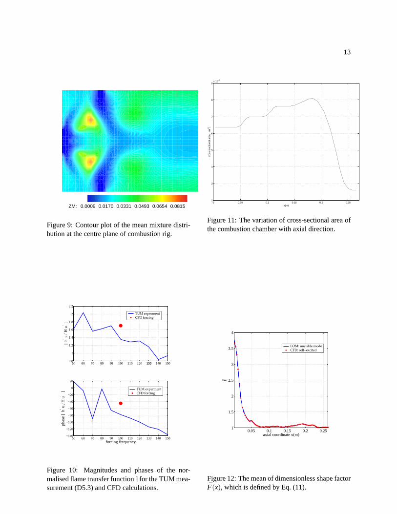
For making the comparison with the experimental work of TUM-LAT (see D5.4), The harmonic forcingcalculation was carried out for CASE W, which the air temperature is 160oC, overall air mass flow rate 50.86g/s and fuel mass flow rate 1.8 g/s. Contour plots of the mean temperature and mixture distribution at thecentre plane of combustion rig are shown in Figs. 8 and 9, respectively. The comparison of the flame transferfunctions at the forcing frequency 100Hz is shown in Fig. 10. Here the overall heat release is considered inthe experimental data. For the calculated transfer function, the heat release is integrated around combustionzone, where corresponding to the measured location in experiment.

For the ‘rumble’ problem we consider here, the convection of non-uniform density or entropy wavethrough the downstream choked nozzle is a significant source of combustion oscillation. The character-istic velocity of non-uniform density gas is the convective speed of fluid particle. For given frequency, itscharacteristic length is much shorter than that of pressure wave. To identify the instability of system, it is de-sirable to have the information of unsteady heat release along the direction of wave propagation. Therefore,the ‘distributed’ transfer function is employed in the low order model. The results of ‘distributed’ transferfunction will be discussed in the next section.

3 Low-Order Models

As the ‘rumble’ problem we consider here is a low frequency oscillation and the wavelengths are long incomparison with the combustor diameter, only plane acoustic waves carry energy. Therefore, it is reasonableto consider one-dimensional disturbance in stability analysis.

3.1 Integrated Properties

We begin by integrating the flow equations over the cross-section. The flow parameters integrated over thecombustor cross-section can be written as

〈φ〉 =1A

∫a φ da, and 〈ψ〉 =

1〈ρ〉A

∫aρψ da, (7)

6

whereφ representsρ andq, and〈ψ〉 representsu, v, u2, et ande. A(x) =∫

da, is the cross-sectional areaof the combustor, and was uniform in our previous 2D study. In the current work, where a more realisticgeometry is considered, the cross-sectional area varies along the axial direction. As shown in Fig. 11, themost apparent variation is that there is a steep lateral contraction near the combustor exit.

Integrating the ensemble averaged conservation equations With the assumption of negligible molecu-lar transport, and negligible Reynolds stresses and fluxes, one-dimensional conservation equations can bewritten as

∂ 〈ρ〉∂ t

+1H

∂

∂x[H〈ρ〉〈u〉] = Sm, (8)

∂

∂ t[〈ρ〉〈u〉]+ 1

H∂

∂x[〈ρ〉〈u〉2HF ] = −dp

dx+Sf , (9)

∂

∂ t[〈ρ〉〈et〉]+

1H

∂

∂x[〈ρ〉〈u〉〈e〉H] = 〈q〉+Se. (10)

whereSm, Sf andSe are the sources terms of mass, momentum and energy due to the primary and secondaryair injections, respectively.

In Eq. (9), the non-uniform influences of momentum transport in the radial direction are consideredthrough a shape factorF , which is defined as

F(x, t) =〈u2〉〈u〉2 . (11)

For the total energy and total enthalpy, the integrated variable can be written as

〈et〉 = cv〈T〉+12〈u〉2F and, 〈e〉 = cp〈T〉J1 +

12〈u〉2J2 . (12)

The dimensionless shape factorsJ1 andJ2 are used to describe the non-uniform influences of the enthalpyand kinetic energy transports in the radial direction, and are defined as

J1(x, t) =〈cpuT〉

〈cp〉〈u〉〈T〉, and, J2(x, t) = 〈u3〉/〈u〉3 , (13)

respectively. Although the heat capacitycp and state equation coefficientRare not uniform within combus-tion chamber as combustion alters the components of flow, we find from our later results that it is accurateenough to treat them as constants.

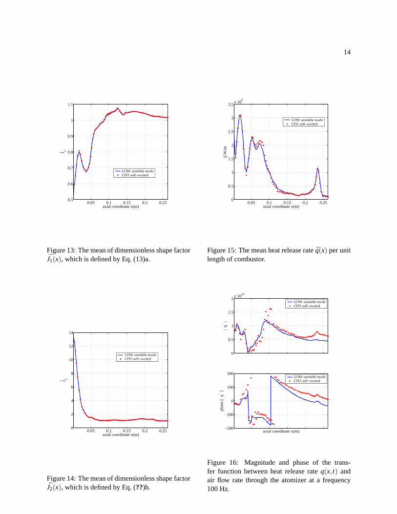
The shape factors (F , J1 andJ2) and the heat release rate〈q〉 can be obtained from a single CFD forcingcalculation. After a steady solution was achieved, the mean values ofF(x), J1(x) andJ2(x) were calculatedaccording to Eqs. (11) and (13), respectively. The results are shown in Figs. 12, 13 and 14, respectively.These non-dimensional shape factors would be unity if the axial velocity and the transported propertieswere ideally uniform. From Fig. 12, it can be seen thatF is large at the combustor inlet due to the high flowvelocities that occur near the injectors with virtually stagnant flow outside the main stream. Elsewhere in thecombustor, the flow is relatively uniform, thusF is closer to unity. The shape factorJ1 is determined not onlyby flow velocity, but also by the temperature distribution. Its mean value is shown in Fig. 13. It is interestedto see thatJ1 is less than unity in the upstream section because here the higher temperature region is locatedin the recirculation zone where the velocity is stagnated or very small. Downstream of the combustion zonethe hot low density gas is differentially accelerated by the pressure gradient andJ1 increases to values greaterthan unity. As a consequence, we can see thatJ1 is continuously increased in Fig. 13. The small steps inFigs. 12-14 correspond to the effects of the primary and secondary air injections. The explanation for theshape factorJ2, which is shown in Fig. 14, is similar to that for Fig. 12. The difference is thatJ2 is muchlarger at the inlet due to the third power of velocity in Eq. (13) for the kinetic energy transport.

7

The integrated mean heat release rate is shown in Fig. 15. It can be seen that the maximum value islocated at the front edge of the recirculation zone, where air/fuel mixing is enhanced by the increase in airvelocity, which increases the shear and hence the turbulence scalar dissipation rate.

3.2 Low-order Model

To consider linear perturbations of one-dimensional flows, it is convenient to write the governing equationsin terms of flux quantities. Here the mass, momentum, and energy fluxes are defined as

m(x, t) = A〈ρ〉〈u〉 , f (x, t) = A(〈p〉+ 〈ρ〉〈u〉2F) and, E(x, t) = A〈ρ〉〈u〉〈e〉 ,

respectively. As the linear perturbation theory is considered here, it is sufficient to investigate perturbationto the mean flow with time dependenceeiωt . The sign of imaginary part ofω determines the stability, whileRe(ω) gives the frequency of the mode. Now time mean values will be denoted by the overbar and flowquantities can be expressed as

φ(x, t) = φ(x)+φ′(x, t) , (14)

where the fluctuating componentφ ′(x, t) = Re(φ(x)eiωt). Compared with Eqs. (8)-(10), the conservationequations for steady flow can be written as

ddx

¯〈m〉 = Sm, (15)

ddx

¯〈 f 〉 = ¯〈p〉dHdx

+ Sf , (16)

ddx

¯〈E〉 = H ¯〈q〉+ Se. (17)

With the definition of Eq. (14) and the equation of state, the relationships for flow variables can bewritten as [4]

¯〈u〉 =γ J1

¯〈 f 〉[2γFJ1− (γ −1)J2] ¯〈m〉

−

[γ2J21

¯〈 f 〉2+2[J2(γ −1)2−2F J1γ(γ −1)] ¯〈m〉 ¯〈E〉] 1

2

[2γF J1− (γ −1)J2] ¯〈m〉, (18)

¯〈p〉 = ( ¯〈 f 〉− ¯〈m〉 ¯〈u〉F)/H , (19)¯〈ρ〉 = ¯〈m〉/(H ¯〈u〉) , (20)¯〈T〉 = ¯〈p〉/(R ¯〈ρ〉) . (21)

whereγ is the ratio of specific heat capacities.For unsteady parts of the mass flux, momentum flux and energy flux, we have

〈m〉′ = H (〈ρ〉′ ¯〈u〉+ ¯〈ρ〉〈u〉′) , (22)

〈 f 〉′ = H [(2 ¯〈ρ〉 ¯〈u〉〈u〉′ + 〈ρ〉′ ¯〈u〉2) F +

¯〈ρ〉 ¯〈u〉2F ′ + 〈p〉′] , (23)

〈E〉′ = H [〈m〉′(cp¯〈T〉J1 +

12

¯〈u〉2J2)+cp

¯〈T〉J′1 +

12

¯〈u〉2J′2 +( ¯〈ρ〉 ¯〈u〉)(cp 〈T〉′J1 + ¯〈u〉〈u〉′J2)] . (24)

8

With the state equation, the perturbation of flow variables can be written as

〈u〉′ = {[0.5(γ −1)J2 + F J1] ¯〈u〉2〈m〉′− J1¯〈u〉〈 f 〉′−

(γ −1)〈E〉′−2HR cp¯〈u〉J′1−H ¯〈p〉 ¯〈ρ〉− ¯〈u〉3

J′2 +

2HR cp¯〈ρ〉 ¯〈u〉3

J1F ′}/{H[ ¯〈p〉J1 + F J1¯〈ρ〉 ¯〈u〉2

+

(γ −1)J2¯〈ρ〉 ¯〈u〉2

]} , (25)

〈ρ〉′ =〈m〉′

H ¯〈u〉−

¯〈ρ〉〈u〉′¯〈u〉

, (26)

〈p〉′ =〈 f 〉′− F( ¯〈u〉〈m〉′ + ¯〈m〉〈u〉′)− ¯〈m〉 ¯〈u〉F ′

H, (27)

〈T〉′ = ¯〈T〉(〈p〉′

¯〈p〉− 〈ρ〉′

¯〈ρ〉) . (28)

For linear disturbances whose time dependence is proportional toeiωt , the equations for the perturbationsof mass flux, momentum flux and energy flux can be written as

d ˆ〈m〉dx

= −iωH ˆ〈ρ〉 , (29)

d ˆ〈 f 〉dx

= −iω ˆ〈m〉+ ˆ〈p〉dHdx

, (30)

ddx

〈E〉 = ˆ〈q〉− iωH[ ˆ〈ρ〉(cv¯〈T〉+ 1

2¯〈u〉2

F)+

¯〈ρ〉(cvˆ〈T〉+ ¯〈u〉 ˆ〈u〉F +

12

¯〈u〉2F)] . (31)

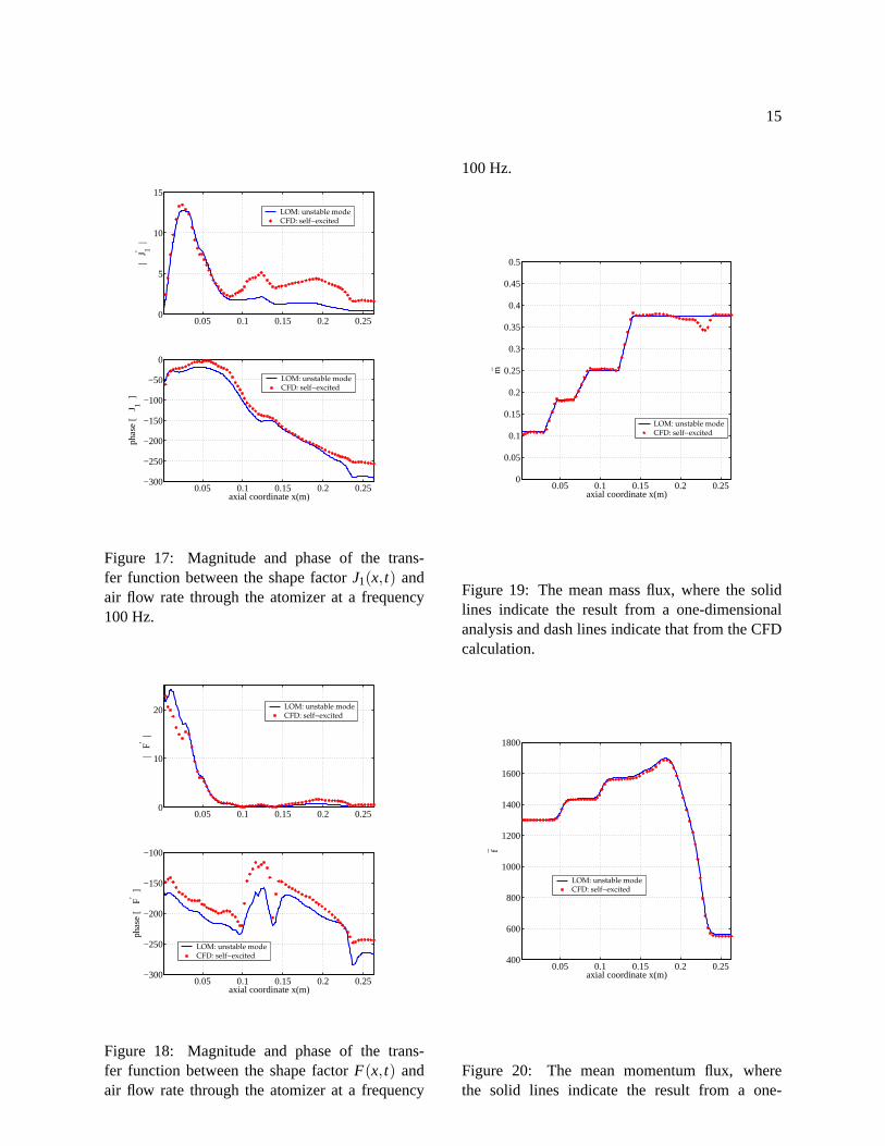
In the one-dimensional analysis, the flame transfer functionˆ〈q〉, which is shown in Fig. 16, describesthe relationship between the unsteady heat release rate with inlet oscillations. We found that this approachled to one-dimensional disturbances which were significantly different from the area-averaged CFD results.Therefore, it is necessary to investigate the sensitivities of the results to the time dependence of the threenon-dimensional shape factors. In Eq. (??), the non-dimensional shape factorJ′1 describes the effects ofoscillation on the shape factor describing non-uniformity of the enthalpy transport in the axial direction.According to the definition, it is determined by both axial velocity and temperature. That means it also hasan influence on the transport of the entropy wave. It is evident from Fig. 17 that the position of maximumamplitude ofJ′1 is in the recirculation zone. This can be explained by the fact that fluctuation in the inlet airnot only alters the fuel vapor distribution in this region, it also alters the vorticity, and thus effects the radialdistribution of enthalpy.J1(x, t) is influenced primarily by the inlet air flow rate andJ1(ω,x)/ma(ω) can beidentified from a single forced CFD calculation as the flame transfer function.

In Eq. (11), F ′ represents the variation of momentum flux when the oscillations changes the non-uniformity of the axial velocity. The magnitude and phase of the relationship betweenF(x, t) and inletair mass flow rate are shown in Fig. 18. It is seen that there is a peak in the magnitude plot, which corre-sponds to the jets induced by inlets 1 and 2. It means that the oscillation alters the size or intensity of thejets or vortex, therefore the axial uniformness of momentum transport. A similar conclusion can be drawnabout the non-dimensional factorJ′2, which represents the effect of oscillation on the uniformness of kineticenergy in the radial direction.

9

3.3 Stability Analysis

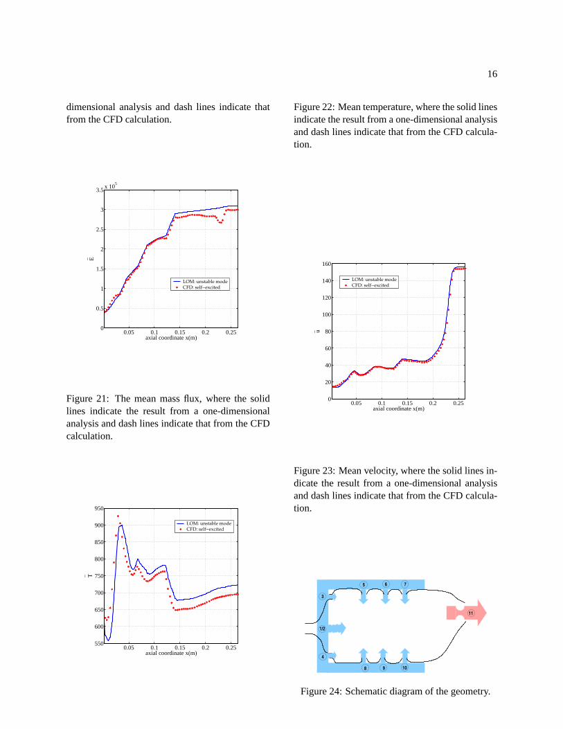
The mean values of mass, momentum and energy fluxes can be calculated through integration of Eqs. (15)-(17) with appropriate inlet boundary conditions. The results are shown in Figs. 19-21 are with inlet boundaryconditions derived from the CFD results to aid comparison in this paper. In these figures, three steps areclearly demonstrated, which correspond to the contributions from the primary and secondary air injections.In current study, the source termsSm, Sf andSe are kept as constants in both the CFD and in the linearanalysis. The mean values of flow variables can be obtained according to Eqs. (18)-(21). The mean valuesof temperature and velocity are shown in Figs 22 and 23, respectively. From Figs. 19-23, we can see that themean flow results from one-dimensional analysis are in good agreement with those from CFD calculations.From Fig. 22, it can be seen that the integrated temperature is much lower than that within combustion zone.This is because, at this idle condition, the temperature of most of the air within combustor is relatively low,although the local temperature can be as high as 2000 K. For the integrated velocity, as shown in Fig. 23,three steps due to additional air injected are clearly demonstrated. The decrease following each step in meanvelocity is the subsequence of the relatively high density of the cool flow in the recirculation induced by theflow injection.

For the perturbation parts, the boundary conditions are kept as same as those used in the CFD self-excitedoscillation calculation. As shown in Fig. 24, in the inlet boundary, only ports 1 and 2 were considered. Itcan be written as

min = A12(ρ12u12+ ρ12u12) (32)

fin = Ain pin +2A12ρ12u12+A12ρ12u212 (33)

Ein = m12(cpT12+ u12u12)+ m12(cpT12+ u212) . (34)

In the outlet, the choking condition gives

pout

pout= 2

uout

uout+

ρout

ρout. (35)

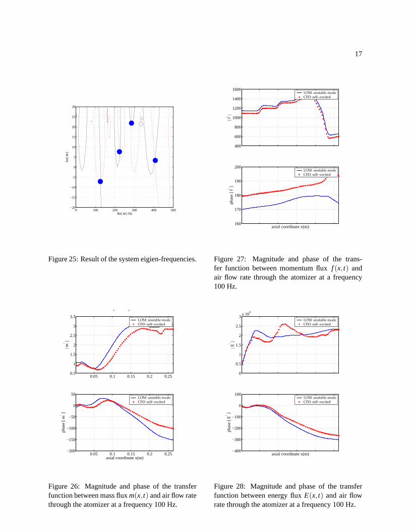
With above boundary conditions, the result of the system eigen-frequencies is shown in Fig. 25. The sign ofimaginary part ofω determines the stability, while real part gives the frequency of the mode. From Fig. 25,we can see that the unstable mode is around 120Hz, and the other modes are stable. It is in good agreementwith that from CFD self-excited oscillation calculation.

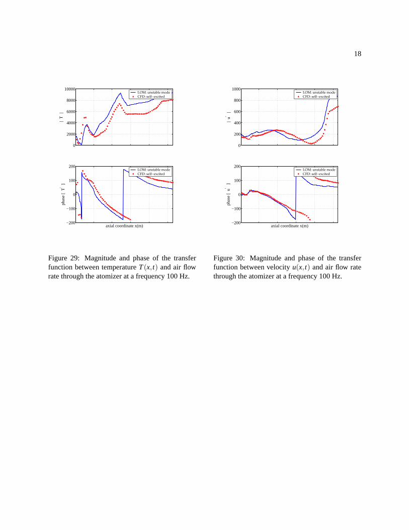
The aim of this study is to develop a method whereby a linear stability analysis can provide a usefultool to predict ‘rumble’. To validate the low-order model, the perturbations of the fluid properties calculatedthrough integration of the integration of Eqs. (22)-(24) are compared with those from CFD self-excitedoscillation calculation. The magnitude and phase of the transfer function between mass, momentum andenergy fluxes and air flow rate through the atomiser at the unstable mode are demonstrated in Figs. 26-28.The results are compared with that from CFD calculation, which is drawn with a dot line. It can be seen thatthe results from the low order model and CFD calculations are in general comparable. With the relationshipsof Eqs. (25)-(28), the perturbation parts of fluid properties can be calculated. The results of temperature andvelocity are shown in Figs. 29-30, respectively.

4 Conclusions

In this work, a new approach is developed to give predications for instability onset and the frequencies ofoscillation. This is based on integrating CFD and low-order models. The CFD provides the transfer func-tion between the heat release rate per unit length and air flow rate through the atomizer by time-dependentcalculations of the combustion processes with specified forced inlet boundary conditions. At the same time

10

the transfer functions between non-dimensional shape factors and inlet air flow rate can be calculated. Byintegrating the ensemble-averaged conservation equations of motion, quasi-one-dimensional equations for alinear stability analysis are derived. The effects of any radial non-uniformity on transport of flow parametersare considered by shape factors, which can be obtained from the same CFD calculation. Flow quantities canbe determined quickly and straightforwardly by solving the mean flow and the linear perturbation equations.The amplitude and phase relationships of temperature and velocity perturbations, which play an importantrole in the downstream boundary condition, have been compared with CFD results for the same inlet bound-ary conditions. The results show good agreement. The strategy outlined here can be expected to have usefulpractical applications if the flame transfer function and the shape factors, determined from a small numberof detailed CFD calculations, can subsequently be applied to linear stability analysis under a wider rangeof conditions. In the future, we will use the method developed here to predict the instability onset and thefrequencies of oscillation. We anticipate the results will be useful to understand the combustion oscillationand be helpful in the development of control strategies.

REFERENCES

[1] M. Zhu, A.P. Dowling, and K.N.C. Bray. Self-excited oscillations in combustors with spray atomisers.Trans. ASME, J. Eng. Gas Turbines Power, 123(779-786), 2001.

[2] M. Zhu, A.P. Dowling, and K.N.C. Bray. Computation of 3D forced combustion oscillation. ICLEACdeliverable report D4.7, September 2002.

[3] F.E. Marble and S.M. Candel. Acoustics disturbances from gas non-uniformities convected through anozzle.Journal of Sound and Vibration, 55(2):225–243, 1977.

[4] A. P. Dowling. The calculation of thermoacoustic oscillations.Journal of Sound and Vibration,180(4):557–581, 1995.

[5] A. P. Dowling. Nonlinear self-excited oscillations of a ducted flame.J. Fluid Mech., 346:271–290,1997.

[6] L. Ljung. System Identification Toolbox User’s Guide. The MathWorks Inc., 1991.

11

X

Y

Z

x = 0.017m

x = 0.038mx = 0.0855m

1

2

3

45

6

7 89

10

Figure 1: Schematic diagram of the gemmetry andgrid distribution

Figure 2: Schematic diagram of the sub-domainused in MPI parallel computing.

100

101

102

10−1

100

101

102

number of processors

elap

sed

time

per

time

step

Sun FirePC Cluster

Figure 3: Schematic diagram of the performance ofparallel computing in PC cluster and SunFire Su-percomputer.

TEMP: 383 509 635 762 888 1014 1141 1267 1393 1519 1646 1772 1898 2025

Figure 4: Contour plot of the mean tempera-ture distribution at the centre plane of combustionchamber at idle condition.

12

T: 365 501 637 774 910 1046 1182 1319 1455 1591 1727 1864 2000

Figure 5: Contour plot the mean temperature dis-tribution of combustion chamber at idle condition.

Figure 6: The time trace of the static pressure ofunsteady CFD calculation with the choking condi-tion.

Figure 7: Close snap of the time trace of thestatic pressure of unsteady CFD calculation withthe choking condition.

TEMP: 449 636 824 1012 1200 1388 1575 1763 1951

Figure 8: Contour plot of the mean temperaturedistribution at the centre plane of combustion rig.

13

ZM: 0.0009 0.0170 0.0331 0.0493 0.0654 0.0815

Figure 9: Contour plot of the mean mixture distri-bution at the centre plane of combustion rig.

50 60 70 80 90 100 110 120 130130 140 1500.8

1

1.2

1.4

1.6

1.8

2

2.2

| h′ u

H

u′ |

50 60 70 80 90 100 110 120 130 140 150−140

−120

−100

−80

−60

−40

−20

0

20

phas

e [

h′ u

H

u′

]

forcing frequency

TUM expermentCFD forcing

TUM expermentCFD forcing

/ /

Figure 10: Magnitudes and phases of the nor-malised flame transfer function ] for the TUM mea-surement (D5.3) and CFD calculations.

0 0.05 0.1 0.15 0.2 0.252

3

4

5

6

7

8

9x 10

−3

x(m) cr

oss−

sect

iona

l are

a

(m2 )

Figure 11: The variation of cross-sectional area ofthe combustion chamber with axial direction.

0.05 0.1 0.15 0.2 0.251

1.5

2

2.5

3

3.5

4

axial coordinate x(m)

F

LOM: unstable modeCFD: self−excited

−

Figure 12: The mean of dimensionless shape factorF(x), which is defined by Eq. (11).

14

0.05 0.1 0.15 0.2 0.250.5

0.6

0.7

0.8

0.9

1

1.1


J1


−

Figure 13: The mean of dimensionless shape factorJ1(x), which is defined by Eq. (13)a.

0.05 0.1 0.15 0.2 0.250

2

4

6

8

10

12

14


J2


−

Figure 14: The mean of dimensionless shape factorJ2(x), which is defined by Eq. (??)b.

0.05 0.1 0.15 0.2 0.250

0.5

1

1.5

2

2.5

3

3.5x 10

8


q W

/m


−

Figure 15: The mean heat release rate ¯q(x) per unitlength of combustor.

0

0.5

1

1.5

2x 10

10

| q′ |


−200

−100

0

100

200

phas

e [

q′ ]



Figure 16: Magnitude and phase of the trans-fer function between heat release rateq(x, t) andair flow rate through the atomizer at a frequency100 Hz.

15

0.05 0.1 0.15 0.2 0.250

5

10

15

| J

1′ |


0.05 0.1 0.15 0.2 0.25−300

−250

−200

−150

−100

−50

0

phas

e [

J 1′ ]



Figure 17: Magnitude and phase of the trans-fer function between the shape factorJ1(x, t) andair flow rate through the atomizer at a frequency100 Hz.

0.05 0.1 0.15 0.2 0.250

10

20

| F

′ |


0.05 0.1 0.15 0.2 0.25−300

−250

−200

−150

−100

phas

e [

F′ ]



Figure 18: Magnitude and phase of the trans-fer function between the shape factorF(x, t) andair flow rate through the atomizer at a frequency

100 Hz.

0.05 0.1 0.15 0.2 0.250

0.05

0.1

0.15

0.2

0.25

0.3

0.35

0.4

0.45

0.5

axial coordinate x(m) m


−

Figure 19: The mean mass flux, where the solidlines indicate the result from a one-dimensionalanalysis and dash lines indicate that from the CFDcalculation.

0.05 0.1 0.15 0.2 0.25400

600

800

1000

1200

1400

1600

1800


f


−

Figure 20: The mean momentum flux, wherethe solid lines indicate the result from a one-

16

dimensional analysis and dash lines indicate thatfrom the CFD calculation.

0.05 0.1 0.15 0.2 0.250

0.5

1

1.5

2

2.5

3

3.5x 10

5


E


−

Figure 21: The mean mass flux, where the solidlines indicate the result from a one-dimensionalanalysis and dash lines indicate that from the CFDcalculation.

0.05 0.1 0.15 0.2 0.25550

600

650

700

750

800

850

900

950


T


−

Figure 22: Mean temperature, where the solid linesindicate the result from a one-dimensional analysisand dash lines indicate that from the CFD calcula-tion.

0.05 0.1 0.15 0.2 0.250

20

40

60

80

100

120

140

160


u


−

Figure 23: Mean velocity, where the solid lines in-dicate the result from a one-dimensional analysisand dash lines indicate that from the CFD calcula-tion.

3

4

5 6 7

8 9 10

11

1/2

Figure 24: Schematic diagram of the geometry.

17

0 100 200 300 400 500−20

−15

−10

−5

0

5

10

15

20

25

30

Re( ω ) Hz

Im(

ω )

. .

. .

Figure 25: Result of the system eigien-frequencies.

0.05 0.1 0.15 0.2 0.250.5

1

1.5

2

2.5

3

3.5

| m′ |


0.05 0.1 0.15 0.2 0.25−200

−150

−100

−50

0

50

phas

e [ m

′ ]



^

^

Figure 26: Magnitude and phase of the transferfunction between mass fluxm(x, t) and air flow ratethrough the atomizer at a frequency 100 Hz.

400

600

800

1000

1200

1400

1600

| f′ |


160

170

180

190

200

phas

e [

f′ ] axial coordinate x(m)


Figure 27: Magnitude and phase of the trans-fer function between momentum fluxf (x, t) andair flow rate through the atomizer at a frequency100 Hz.

0

0.5

1

1.5

2

2.5

3x 10

6

| E′ |


−400

−300

−200

−100

0

100

phas

e [ E

′ ]



Figure 28: Magnitude and phase of the transferfunction between energy fluxE(x, t) and air flowrate through the atomizer at a frequency 100 Hz.

18

0

2000

4000

6000

8000

10000

| T

′ |


−200

−100

0

100

200

phas

e [

T′ ]



Figure 29: Magnitude and phase of the transferfunction between temperatureT(x, t) and air flowrate through the atomizer at a frequency 100 Hz.

0

200

400

600

800

1000

| u′

|


−200

−100

0

100

200

phas

e [

u′ ]



Figure 30: Magnitude and phase of the transferfunction between velocityu(x, t) and air flow ratethrough the atomizer at a frequency 100 Hz.

Documents

ICLEAC CONTRACT N : G4RD-CT2000-0215 PROJECT N · PDF fileInstability Control of Low Emission Aero-engine Combustors ... In a previous study, ... the mathematical models and dynamic