UNIVERSITA DEGLI STUDI DI PADOVA

Dipartimento di ingegneria industriale

Corso di Laurea Magistrale in Ingegneria Aerospaziale

Tesi di Laurea

Ice accretion simulation over 2Dairfoils by means of a methodology

embedded in a CFD solver

Stefano Fornasier

Relatore:Prof. Ernesto Benini

Correlatore:Ing. Elisabetta Borghi

Anno Accademico 2015 - 2016

Abstract

The analytical investigation of ice accretion is a complementary part of flight andwind tunnel tests needed for certification and ice protection system design. Because thecomputational fluid dynamics is usually limited to the flow solutions over iced surfacesthe actual icing simulations generally relies on potential flow solution.

In this thesis the ice accretion over bi dimensional aerodynamic surfaces is performedfor a wide variety of conditions. A dedicated tool, IceMAP 2D, has been developed tointegrate the ice accretion simulation process in the CFD software Fluent, used to solvethe compressible Navier-Stokes equations.

The tool developed has been validated with experimental data and icing software indemanding conditions; also the effects of varying different parameters, like velocity or tem-perature, on the ice shape has been investigated. Finally the aerodynamic characteristicsof iced airfoil have been studied and compared with experimental data.

i

Contents

1 Introduction 11.1 Icing in helicopter operations . . . . . . . . . . . . . . . . . . . . . . . . . 31.2 Literature review . . . . . . . . . . . . . . . . . . . . . . . . . . . . . . . . 61.3 Icing codes . . . . . . . . . . . . . . . . . . . . . . . . . . . . . . . . . . . . 6

2 Physics of ice accretion 82.1 Icing parameters . . . . . . . . . . . . . . . . . . . . . . . . . . . . . . . . 8

2.1.1 Temperature . . . . . . . . . . . . . . . . . . . . . . . . . . . . . . . 82.1.2 Liquid water content . . . . . . . . . . . . . . . . . . . . . . . . . . 92.1.3 Droplet size . . . . . . . . . . . . . . . . . . . . . . . . . . . . . . . 92.1.4 Airspeed . . . . . . . . . . . . . . . . . . . . . . . . . . . . . . . . . 10

2.2 Aerodynamic solution . . . . . . . . . . . . . . . . . . . . . . . . . . . . . . 102.3 Droplets trajectories computation . . . . . . . . . . . . . . . . . . . . . . . 11

2.3.1 Collection efficiency . . . . . . . . . . . . . . . . . . . . . . . . . . . 132.4 Energy and mass balance . . . . . . . . . . . . . . . . . . . . . . . . . . . . 14

2.4.1 Ice temperature . . . . . . . . . . . . . . . . . . . . . . . . . . . . . 19

3 Numerical tool: IceMAP 2D 213.1 Procedure for ice accretion computation . . . . . . . . . . . . . . . . . . . 21

3.1.1 Workbench . . . . . . . . . . . . . . . . . . . . . . . . . . . . . . . 243.1.2 UDF development . . . . . . . . . . . . . . . . . . . . . . . . . . . . 25

3.2 Geometry and Mesh . . . . . . . . . . . . . . . . . . . . . . . . . . . . . . 273.2.1 Mesh creation . . . . . . . . . . . . . . . . . . . . . . . . . . . . . . 293.2.2 Mesh refinement . . . . . . . . . . . . . . . . . . . . . . . . . . . . 33

3.3 Heat Transfer Coefficient . . . . . . . . . . . . . . . . . . . . . . . . . . . . 363.3.1 Effect of surface roughness . . . . . . . . . . . . . . . . . . . . . . . 373.3.2 Effect of turbulence model . . . . . . . . . . . . . . . . . . . . . . . 413.3.3 Thermal boundary conditions . . . . . . . . . . . . . . . . . . . . . 46

3.4 Flow field computation . . . . . . . . . . . . . . . . . . . . . . . . . . . . . 533.5 Particle tracking . . . . . . . . . . . . . . . . . . . . . . . . . . . . . . . . 57

3.5.1 Particle initialization . . . . . . . . . . . . . . . . . . . . . . . . . . 573.5.2 Collection efficiency . . . . . . . . . . . . . . . . . . . . . . . . . . . 58

3.6 Thermodynamic balance . . . . . . . . . . . . . . . . . . . . . . . . . . . . 643.7 Accretion algorithm . . . . . . . . . . . . . . . . . . . . . . . . . . . . . . . 653.8 Mesh modification and control . . . . . . . . . . . . . . . . . . . . . . . . . 67

ii

4 Results 704.1 Time step selection . . . . . . . . . . . . . . . . . . . . . . . . . . . . . . . 714.2 IceMAP 2D validation . . . . . . . . . . . . . . . . . . . . . . . . . . . . . 71

5 Computation of aerodynamic coefficients 985.1 Rime conditions . . . . . . . . . . . . . . . . . . . . . . . . . . . . . . . . . 985.2 Glaze conditions . . . . . . . . . . . . . . . . . . . . . . . . . . . . . . . . . 99

6 Conclusions 104

7 Future development 105

Appendix:

A IceMAP 2D structure 107A.1 List of input . . . . . . . . . . . . . . . . . . . . . . . . . . . . . . . . . . . 107A.2 Solution steps . . . . . . . . . . . . . . . . . . . . . . . . . . . . . . . . . . 109A.3 List of output . . . . . . . . . . . . . . . . . . . . . . . . . . . . . . . . . . 111A.4 Postprocessing . . . . . . . . . . . . . . . . . . . . . . . . . . . . . . . . . . 114

iii

List of Figures

1.1 Rime ice accretion, left, and glaze ice, right. . . . . . . . . . . . . . . . . . 21.2 Ice accumulation on aircraft wing. . . . . . . . . . . . . . . . . . . . . . . . 21.3 Icing on an external probe. . . . . . . . . . . . . . . . . . . . . . . . . . . . 41.4 Top left: Ice detector, used to detect the presence of liquid water in the air.

Bottom right: SLD marker, provides visual information on particle size; ifice grows in the red or yellow area particle size is above certification limits,and flight is not permitted. . . . . . . . . . . . . . . . . . . . . . . . . . . . 5

1.5 AW139 during icing trials; a CH-47 sprays liquid water which reproduceicing conditions, while the tested helicopter follows. . . . . . . . . . . . . . 6

2.1 Influence of ambient conditions on ice shapes. . . . . . . . . . . . . . . . . 92.2 Differences in particle trajectories, diameter 10 µm (left) and 40 µm (right). 102.3 Definition of total and local collection efficiency. . . . . . . . . . . . . . . . 132.4 Identification of the control volumes over each segment defining the body. . 142.5 Mass balance for each control volume. 1: impinging water; 2: water leaving

the airfoil through evaporation or sublimation; 3: runback water leavingthe control volume; 4: runback water entering the control volume; 5: waterleaving the control volume through icing. . . . . . . . . . . . . . . . . . . 15

3.1 Illustration of the solution process with IceMAP 2D. . . . . . . . . . . . . 223.2 Ice accretion module, implemented in Fluent using user defined functions. . 233.3 ANSYS Workbench project schematic. . . . . . . . . . . . . . . . . . . . . 243.4 Solution process of Fluent with UDFs. Image from [3]. . . . . . . . . . . . 263.5 Domain and mesh used. The airfoil is at the centre of the domain. . . . . . 273.6 Mesh for a clean airfoil NACA0015. Unstructured, triangular mesh. . . . 283.7 Mesh for an iced NACA0015; detail of mesh elements near the leading edge

of the clean airfoil. . . . . . . . . . . . . . . . . . . . . . . . . . . . . . . . 293.8 Impinging water on clean and iced airfoil, element size 0.1 mm, no smoothing. 303.9 Impinging water on a clean NACA0012 airfoil, mesh size 0.1 mm and 2 mm. 303.10 Ice shape with mesh size of 0.1 mm and 2 mm. . . . . . . . . . . . . . . . 313.11 Effect of mesh size on ice accretion. Mesh size: 2 mm left, 4 mm right. . . 323.12 Detail of the mesh used for ice accretion. Element size 2 mm. . . . . . . . 323.13 Detail of the mesh used for aerodynamic purpose. Element size 0.1 mm. . 333.14 Tgrid in the project schematic of ANSYS Workbench. . . . . . . . . . . . . 343.15 Mesh near horns, Tgrid top and ANSYS Meshing bottom. . . . . . . . . . 343.16 Mesh on iced airfoil, Tgrid top and ANSYS Meshing bottom. . . . . . . . . 353.17 Heat transfer coefficient computed with different roughness and turbulence

model. . . . . . . . . . . . . . . . . . . . . . . . . . . . . . . . . . . . . . . 36

iv

3.18 Ice accretion with different heat transfer coefficient. . . . . . . . . . . . . . 363.19 Dense roughness pattern on airfoil. Location identified by the number,

with 1 = -0.036 s/c and 12 = 0.095 s/c. Heat transfer coefficient measuredat 0◦ and 4◦. . . . . . . . . . . . . . . . . . . . . . . . . . . . . . . . . . . . 37

3.20 Sparse roughness pattern on airfoil. Location identified by the number,with 1 = -0.036 s/c and 12 = 0.095 s/c. Heat transfer coefficient measuredat 0◦. . . . . . . . . . . . . . . . . . . . . . . . . . . . . . . . . . . . . . . . 37

3.21 Heat transfer coefficient measured in flight for smooth and roughened NACA0012, angle of attack 0 ◦. Two roughness pattern used. Data from [12]. . . 38

3.22 Heat transfer coefficient measured in flight for smooth and roughened NACA0012, angle of attack 4 ◦. Data from [12]. . . . . . . . . . . . . . . . . . . . 38

3.23 Heat transfer coefficient for a smooth and rough NACA 0012; the final iceshape with the different values of htc is visible in figure 3.24 and 3.25. . . . 39

3.24 With surface roughness. . . . . . . . . . . . . . . . . . . . . . . . . . . . . 403.25 Without surface roughness. . . . . . . . . . . . . . . . . . . . . . . . . . . . 403.26 Illustration of the equivalent sand grain roughness concept employed in

Fluent. . . . . . . . . . . . . . . . . . . . . . . . . . . . . . . . . . . . . . . 413.27 Heat transfer coefficient computed with kε− realizable and SST model. . 423.28 kε− realizable turbulence model used to compute heat transfer coefficient. 433.29 SST turbulence model used to compute heat transfer coefficient. . . . . . . 433.30 Frossling number for a smooth airfoil, flight and wind tunnel data compared

with Fluent. Reynolds number approximately 1280000. . . . . . . . . . . . 443.31 Icing Research Tunnel data compared with Fluent and integral boundary

layer solution. . . . . . . . . . . . . . . . . . . . . . . . . . . . . . . . . . . 443.32 Heat transfer coefficient computed with different turbulence model and

compared with LEWICE. . . . . . . . . . . . . . . . . . . . . . . . . . . . 463.33 Heat transfer coefficient computed with fixed surface temperature and cor-

rect temperature distribution. Free stream temperature 254.15 K. . . . . . 473.34 Temperature distribution on the surface of the airfoil. Free stream temper-

ature 254.15 K. . . . . . . . . . . . . . . . . . . . . . . . . . . . . . . . . . 473.35 Fixed heat flux used to compute htc, AoA = 0◦. . . . . . . . . . . . . . . . 493.36 Fixed heat flux used to compute htc, AoA = 4◦. . . . . . . . . . . . . . . . 493.37 Surface temperature near the leading of a NACA 0012 airfoil; heat flux

50000 W/(m2K), AoA = 0 ◦. . . . . . . . . . . . . . . . . . . . . . . . . . 503.38 Fixed surface temperature used to compute htc, AoA = 0◦. . . . . . . . . . 503.39 Fixed surface temperature used to compute htc, AoA = 4◦. . . . . . . . . . 513.40 Fixed surface temperature used to compute heat transfer coefficient, T∞ =

270 K. . . . . . . . . . . . . . . . . . . . . . . . . . . . . . . . . . . . . . . 523.41 Example of pressure far field settings in Fluent. . . . . . . . . . . . . . . . 533.42 Pressure field around a 22.5 minutes ice shape on the Twin Otter tail; angle

of attack 0◦, free stream velocity 90 m/s, pressure 97216 Pa. . . . . . . . . 533.43 Velocity flow field around a 22.5 minutes ice shape on the Twin Otter tail;

angle of attack 0◦, free stream velocity 90 m/s, pressure 97216 Pa. . . . . 543.44 Coefficient of pressure on the Twin Otter horizontal tail; angle of attack

0◦, free stream velocity 78.23 m/s, pressure 99974 Pa. . . . . . . . . . . . 55

v

3.45 Coefficient of pressure on a simulated 22.5 minutes ice shape on the TwinOtter horizontal tail; angle of attack 0◦, free stream velocity 90 m/s, pres-sure 97216 Pa. . . . . . . . . . . . . . . . . . . . . . . . . . . . . . . . . . 56

3.46 Coefficient of pressure on a clean GLC 305 airfoil; angle of attack 1.5◦, freestream velocity 78.23 m/s, pressure 98732 Pa. . . . . . . . . . . . . . . . . 56

3.47 List of particle properties. These are set using a UDF. . . . . . . . . . . . 583.48 GLC305 collection efficiency for 11 µm MVD. . . . . . . . . . . . . . . . . 603.49 GLC305 collection efficiency for 21 µm MVD. . . . . . . . . . . . . . . . . 613.50 Collection efficiency for 11 µm MVD on the Twin Otter horizontal tail

section. . . . . . . . . . . . . . . . . . . . . . . . . . . . . . . . . . . . . . . 613.51 Collection efficiency for 21 µm MVD on the Twin Otter horizontal tail

section. . . . . . . . . . . . . . . . . . . . . . . . . . . . . . . . . . . . . . . 623.52 Collection efficiency for 11 µm MVD on a simulated 22.5 minutes ice shape

on the Twin Otter horizontal tail section. . . . . . . . . . . . . . . . . . . . 623.53 Collection efficiency for 21 µm MVD on a simulated 22.5 minutes ice shape

on the Twin Otter horizontal tail section. . . . . . . . . . . . . . . . . . . . 633.54 Collection efficiency for 79 µm MVD on a simulated 22.5 minutes ice shape

on the Twin Otter horizontal tail section. . . . . . . . . . . . . . . . . . . . 633.55 Illustration of ice accretion procedure. . . . . . . . . . . . . . . . . . . . . 653.56 Illustration of the procedure to remove intersections. . . . . . . . . . . . . 663.57 Example of mesh morphed in Fluent, with highly skewed cells and negative

volumes. . . . . . . . . . . . . . . . . . . . . . . . . . . . . . . . . . . . . . 673.58 Domain remeshed, satisfying the quality requirements. . . . . . . . . . . . 68

4.1 NACA0012 airfoil in adimensional coordinates. . . . . . . . . . . . . . . . . 714.2 NACA0015 airfoil in adimensional coordinates. . . . . . . . . . . . . . . . . 714.3 GLC305 airfoil in adimensional coordinates. . . . . . . . . . . . . . . . . . 724.4 Run: rime. NACA0012, V∞ = 67.056 m/s, T∞ = 246.15 K, AOA = 0◦,

LWC = 0.99 g/m3, MVD = 38 µm, t = 7 min. . . . . . . . . . . . . . . . 744.5 Coefficient of pressure on iced airfoil for run rime computed with two dif-

ferent meshes and compared with LEWICE. . . . . . . . . . . . . . . . . . 744.6 Run: rime. NACA0012, V∞ = 67.056 m/s, T∞ = 254.15 K, AOA = 0◦,

LWC = 0.99 g/m3, MVD = 38 µm, t = 7 min. . . . . . . . . . . . . . . . 754.7 Coefficient of pressure for final ice shape compared with LEWICE. . . . . . 754.8 Run: rime. NACA0012, V∞ = 67.056 m/s, T∞ = 262.15 K, AOA = 0◦,

LWC = 0.99 g/m3, MVD = 38 µm, t = 7 min. . . . . . . . . . . . . . . . 764.9 Coefficient of pressure for final ice shape compared with LEWICE. . . . . . 764.10 Run: 425. NACA0012, V∞ = 67.1 m/s, T∞ = 244.51 K, AOA = 4◦, LWC

= 1 g/m3, MVD = 20 µm, t = 6 min. . . . . . . . . . . . . . . . . . . . . 784.11 Run: 11. NACA0012, V∞ = 67.056 m/s, T∞ = 253.69 K, AOA = 4◦,

LWC = 1 g/m3, MVD = 20 µm, t = 6 min. . . . . . . . . . . . . . . . . . 794.12 Run: 112. NACA0012, V∞ = 67.056 m/s, T∞ = 259.8 K, AOA = 4◦,

LWC = 1 g/m3, MVD = 20 µm, t = 6 min. . . . . . . . . . . . . . . . . . 794.13 Run: 118. NACA0012, V∞ = 67.056 m/s, T∞ = 263.14 K, AOA = 4◦,

LWC = 1 g/m3, MVD = 20 µm, t = 6 min. . . . . . . . . . . . . . . . . . 80

vi

4.14 Run: 122. NACA0012, V∞ = 67.056 m/s, T∞ = 265.35 K, AOA = 4◦,LWC = 1 g/m3, MVD = 20 µm, t = 6 min. . . . . . . . . . . . . . . . . . 80

4.15 Run: 421. NACA0012, V∞ = 67.1 m/s, T∞ = 268.4 K, AOA = 4◦, LWC= 1 g/m3, MVD = 20 µm, t = 6 min. . . . . . . . . . . . . . . . . . . . . 81

4.16 Run: 405. NACA0012, V∞ = 102.8 m/s, T∞ = 250.37 K, AOA = 4◦,LWC = 0.55 g/m3, MVD = 20 µm, t = 7 min. . . . . . . . . . . . . . . . 83

4.17 Run: 5512. NACA0012, V∞ = 102.8 m/s, T∞ = 256.78 K, AOA = 4◦,LWC = 0.55 g/m3, MVD = 20 µm, t = 7 min. . . . . . . . . . . . . . . . 84

4.18 Run: 403. NACA0012, V∞ = 102.8 m/s, T∞ = 262.04 K, AOA = 4◦,LWC = 0.55 g/m3, MVD = 20 µm, t = 7 min. . . . . . . . . . . . . . . . 84

4.19 Run: 5528. NACA0012, V∞ = 102.8 m/s, T∞ = 265.67 K, AOA = 4◦,LWC = 0.55 g/m3, MVD = 20 µm, t = 7 min. . . . . . . . . . . . . . . . 85

4.20 Run: 411. NACA0012, V∞ = 102.8 m/s, T∞ = 262.04 K, AOA = 4◦,LWC = 0.55 g/m3, MVD = 20 µm, t = 14 min. . . . . . . . . . . . . . . . 87

4.21 Run: 403. NACA0012, V∞ = 102.8 m/s, T∞ = 262.04 K, AOA = 4◦,LWC = 0.55 g/m3, MVD = 20 µm, t = 7 min. . . . . . . . . . . . . . . . 87

4.22 Run: DRA37. NACA0012, V∞ = 130.5 m/s, T∞ = 260.7 K, AOA = 0◦,LWC = 0.5 g/m3, MVD = 17.5 µm, t = 2 min. . . . . . . . . . . . . . . . 89

4.23 Run: DRA38. NACA0012, V∞ = 130.5 m/s, T∞ = 260.7 K, AOA = 8.5◦,LWC = 0.5 g/m3, MVD = 17.5 µm, t = 2 min. . . . . . . . . . . . . . . . 89

4.24 Run: 412. NACA0012, V∞ = 102.8 m/s, T∞ = 261.54 K, AOA = 4◦,LWC = 0.47 g/m3, MVD = 30 µm, t = 8.2 min. . . . . . . . . . . . . . . 90

4.25 Run: 406. NACA0012, V∞ = 102.8 m/s, T∞ = 264.37 K, AOA = 4◦,LWC = 0.4 g/m3, MVD = 20 µm, t = 9.8 min. . . . . . . . . . . . . . . . 91

4.26 Run: 624963. NACA0015, V∞ = 95.215 m/s, T∞ = 262.85 K, AOA = 0◦,LWC = 0.75 g/m3, MVD = 19 µm, t = 10 min. . . . . . . . . . . . . . . . 93

4.27 Run: 624966. NACA0015, V∞ = 85.39 m/s, T∞ = 263.07 K, AOA = 0◦,LWC = 0.77 g/m3, MVD = 23.4 µm, t = 10.8 min. . . . . . . . . . . . . . 93

4.28 Run: 072701. GLC305, V∞ = 90 m/s, T∞ = 263.2 K, AOA = 6◦, LWC= 0.43 g/m3, MVD = 20 µm, t = 45 min. . . . . . . . . . . . . . . . . . . 95

4.29 Run: 072703. GLC305, V∞ = 90 m/s, T∞ = 263.2 K, AOA = 6◦, LWC= 0.6 g/m3, MVD = 15 µm, t = 22.5 min. . . . . . . . . . . . . . . . . . . 95

4.30 Run: AW5. AW airfoil, V∞ = 92.6 m/s, T∞ = 270.15 K, AOA = -2.5◦,LWC = 0.63 g/m3, MVD = 25 µm, t = 15 min. . . . . . . . . . . . . . . . 97

5.1 Final ice shape obtained for rime ice, Fluent and IRT. . . . . . . . . . . . . 995.2 Plot of coefficient of drag vs AoA for rime ice, Fluent and IRT. . . . . . . . 1005.3 Ice shape obtained for glaze condition, IceMAP 2D and IRT. . . . . . . . . 1005.4 Plot of coefficient of drag vs AoA for glaze ice, Fluent and IRT. . . . . . . 1015.5 Coefficient of lift for a clean and iced NACA 0012 airfoil. . . . . . . . . . . 1025.6 Vectors of velocity on the upper surface of the iced airfoil. Recirculation

of flow over a large area at 5.5 degrees on a glaze ice accretion. . . . . . . . 103

A.1 User inputs required. . . . . . . . . . . . . . . . . . . . . . . . . . . . . . . 108A.2 Launching of the script in ANSYS Workbench. Also visible below the

blocks that will be created. . . . . . . . . . . . . . . . . . . . . . . . . . . . 109

vii

A.3 Ice shape at different time steps for run 5528. Total accretion time 7minutes, time step of 1 minutes. . . . . . . . . . . . . . . . . . . . . . . . . 114

A.4 Impinging mass flux at different time steps for run 5528. Total accretiontime 7 minutes, time step of 1 minutes. . . . . . . . . . . . . . . . . . . . . 115

A.5 Convective heat flux at different time steps for run 5528. Total accretiontime 7 minutes, time step of 1 minutes. . . . . . . . . . . . . . . . . . . . . 116

viii

Nomenclature

α Angle [rad]

β Collection efficiency

δs Infinitesimal surface length [m]

δy Forward projection of surface length [m]

m Mass flow rate [kg

s]

γ Ratio of specific heat

µ Dynamic viscosity [Pa · s]

ρ Density [kg

m3]

τ Droplet relaxation time

Θ Angle [rad]

A Area [m2]

b Thickness [m]

CD Coefficient of drag

chord Chord length [m]

cp Specific heat [J

kg ·K]

d Diameter [µ ·m]

Dv Diffusivity of water vapour in air [m2

s]

ds Surface area [m2]

E Total collection efficiency

F Force [N ]

Fr Frossling number

ix

g Gravity acceleration [m

s2]

H Forward projection of the airfoil height [m]

Hc Heat transfer coefficient [W

m2 ·K]

Hg Mass transfer coefficient [kg ·KJ

]

k Thermal conductivity [W

m ·K]

ks Equivalent sand grain roughness [m]

L Latent heat [J

kg]

LWC Liquid Water Content [g

m3]

M Mach number

m Mass [kg]

MVD Mean Volumetric diameter [µm]

n Freezing fraction

Nu Nusselt number

p Pressure [Pa]

pwi Vapour pressure of water over ice [Pa]

pww Vapour pressure of water at the surface [Pa]

pw Vapour pressure of water in the atmosphere [Pa]

Pr Prandtl number

q Power [W ]

R Gas constant

Re Reynolds number

S Effective temperature (Sutherland constant) [K]

Sc Schmidt number

T Temperature [K]

t Time [s]

x

V Velocity [m

s]

x Position [m]

y Surface length, position [m]

CFD Computational Fluid Dynamics

CMI Continuous Maximum Icing

DERA Defence Evaluation and Research Agency

FAR Federal Aviation Regulations

FIPS Full Ice Protection System

IMI Intermittent Maximum Icing

JAR Joint Aviation Requirements

LEWICE LEWis ICE accretion program

ONERA Office National d’Etudes et de Recherches Aerospatiales

RANS Reynolds Averaged Navier Stokes equations

SLD Super-cooled Large Droplets

UDF User Defined Functions

Subscripts

(i) Control volume

(i+1) Next control volume

(i−1) Preceding control volume

(t) Current time step

(t+1) Next time step

0 Initial condition

∞ Freestream condition

impact Impact condition

a Aerodynamic

c Convection

d Droplet

edge Edge of the boundary layer

xi

e Evaporation

f Freezing

ice Ice

imp Impinging

i Local

k Kinetic

max Maximum value

min Minimum value

node Node value

p Particle

rb in Runback in

rb out Runback out

ref Reference condition

surf Surface

s Sublimation

v Vaporization, vapour

w Water

xii

xiii

Chapter 1

Introduction

Ice accretion on aerodynamic surfaces, rotors and other components poses a significantissue to the safety of flight; indeed, large areas are exposed to icing, and the risks associatedvary depending on where the ice forms. Issues are mainly due to the altered characteristicsof wings and other aerodynamic surfaces, and the increase in weight due to the mass ofice.

The performance of wings suffers degradation, with increased drag combined with adecrease in lift, and their combined effect may result in premature stall; rotor blades alsosuffer from the weight increase, which may cause abnormal vibrations. Icing on air in-takes can severely disturb the incoming air flow and cause malfunctioning or shutdowns;air intakes are also subject to ice ingestion, with similar consequences. Accretion of iceon the fuselage increases the overall drag, but also impacts the functionality of the instru-mentation, e.g. pitot tubes, and pilots visibility, which may be impeded by icing growingon windshields. Additionally, control surfaces may get stuck or experience limitations intheir movements.

Icing occurs in flight when liquid water droplets present in the air impact on rotorcraftor aircraft and freeze, remaining attached to the surface. This is possible during encounterswith clouds and fog, which are composed by small particles of liquid water, snow flakesor ice crystals; indeed, it has been observed that liquid water can be found in normalenvironmental conditions at temperature up to -40 ◦C. Unlike water droplets, snow andice crystal do not pose a threat for icing, because after impacting they do not remainattached to the surface but return in the air.

Depending on ambient conditions, the ice accretion can be divided in two main typolo-gies, rime and glaze. Rime ice grows when water droplets freeze completely on impact,and assumes a white opaque color (because of the presence of air in the frozen water)and is relatively streamlined. Surface roughness is increased compared with the cleansurface and aerodynamic properties are reduced. Rime ice forms at a combination of lowtemperature, low speed and low liquid water content, and is visible on the left of figure1.1.

At a combination of high temperature, high speed and liquid water content water doesnot freeze completely on impact and flows over the body; the water film flowing on thesurface may eventually freeze further aft and result in localized ice accretion, producingshapes similar to horns. This type of ice accretion is termed glaze ice (figure 1.1, right),and appears translucent and has a significant surface roughness.

1

Figure 1.1: Rime ice accretion, left, and glaze ice, right.

At intermediate conditions ice presents characteristic of both type of ice, with a glazelike accretion limited in area near the leading edge of the airfoil.

To cope with the risks associated with icing two categories of systems are commonlyused, which aim at reducing, in the case of de-icing, or preventing, for anti-icing, theaccretion of ice. In the case of de-icing a limited amount of ice is allowed to grow be-fore being removed, using for example pneumatic systems to break the ice or electricalheater. Anti-icing is necessary for surface that must be kept completely clean from ice,like windshields and pitot tubes, and is often obtained using electrical heater.

Figure 1.2: Ice accumulation on aircraft wing.

Because of the breadth of issues described, icing has been long recognized as a severe

2

hazard to safe flight, as has been highlighted by many accidents. A great effort has beenplaced on identifying the underlying causes of icing, in order to better determine the iceaccretion characteristics and the effects on aircraft and helicopters, as well as to optimizethe functionality of ice protection systems. As a result, many tools have been developedto simulate ice accretion, and this has allowed not to rely solely on flight and wind tunneltesting in the design and certification process of aircraft and helicopters.

The aim of this thesis is to develop a code to simulate ice accretion on bidimensionalbodies, including helicopter blade airfoils. The ice accretion code is embedded in a CFDsoftware, Fluent R©1, in order to take full advantage of the flow field solution computedsolving Navier-Stokes equations. Indeed, the variables required to perform the ice accre-tion simulation have been derived from the flow field solution and the particle trackingmodel. Also a routine to update the geometry and adapt the mesh based on ice accretionhas been developed and integrated within Fluent.

In the following sections a more thorough examination of the effects of icing in heli-copter operations is presented, in order to provide additional insight on the conditionsthat lead to ice formation and the effect of icing peculiar to helicopters. A review ofprevious work and the implementation in icing codes follows.

In the second chapter the mathematical model, used to simulate ice accretion, isdescribed; this includes the description of the parameters that governs ice accretion, theimportance of the aerodynamic solution, the determination of particle trajectories and thethermodynamic solution. The third chapter describes the code developed, IceMAP 2Dand how the model previously described has been implemented. The following chapterspresents the results obtained, in particular the simulated ice shapes, which are comparedwith experimental shapes and other icing software, and the aerodynamic properties oficed airfoil. Conclusions and possible improvements to the model and the tool are thendiscussed.

1.1 Icing in helicopter operations

Rotorcraft are more and more required to fly in all weather conditions, in order tomeet customer needs. A specific type certificate is required for a rotorcraft to fly in icingconditions, otherwise it is forced on ground whenever ice conditions are forecasted. Theaccretion of ice on helicopter surfaces can compromise the success of mission, affectingthe efficiency or worse the safety of the flight. The mass of ice growing on helicopterfuselage causes a weight and drag increase, which translates in greater fuel consumptionand consequently reduced maximum range. The ice mass can also introduce additionalloads and vibrations, causing structural problems.

Helicopter performances are restricted mainly by the accretion of ice on the leadingedge of the main rotor blades, which modify the lift, drag and moment characteristicsof the airfoil. Because of the altered aerodynamic characteristics, an increase in powermay be required to maintain the same flight condition, and may also be accompanied byvibrations and different handling characteristics, that is also the result of the weight of

1ANSYS, ANSYS Workbench, AUTODYN, CFX, FLUENT and any and all ANSYS, Inc. brand,product, service and feature names, logos and slogans are registered trademarks or trademarks of ANSYS,Inc. or its subsidiaries in the United States or other countries. All other brand, product, service andfeature names or trademarks are the property of their respective owners.

3

Figure 1.3: Icing on an external probe.

the ice formation on the blades. Consequently, the loads on the airframe and transmissionincrease, and require monitoring, at least in the certification process, to ensure that theyremain acceptable.

Because of the high loads (aerodynamics and dynamic) experienced during the bladesmotion, ice may break and its pieces be projected in the air; after shedding the surfacegenerally return clean from ice, but it can also result in asymmetric distribution of the icemass, which further increase the level of vibrations. Centrifugal and dynamic forces, aero-dynamic pressure distribution, blade deformations and vibrations, ice structural strengthand local non uniformities and cohesion between ice and blade surface: all these fac-tors contribute to determine the ice shedding process, and make the modelling of thephenomenon extremely difficult. Additionally, ice shedding from blades may impact thefuselage or other system and cause damage to the airframe.

Beside the overall increase in drag, fuselage icing has additional consequence on heli-copter operations. Pilot’s visibility may be impeded by icing on windshiels, and icing onexternal sensors and instrumentation can cause impaired data acquisition. Icing on engineintakes and nacelles can result in engine failure, because of ice ingestion or blockage ofthe airflow.

The ability to fly in known icing conditions could dramatically increase the envelopeof rotorcraft, but requires accurate knowledge of where ice will form, so that adequateice protection systems can be fitted. Because of the large costs involved in the design,build and certification process, only some helicopter are certified for flight onto knownicing conditions, having a Full Ice Protection System installed. Ice protection systemsprovide the pilots with information regarding the icing conditions, with reliable values ofliquid water content, temperature, and visual clues on particle size, and protect the areasof the helicopter more exposed to icing. Ice protection system is activated when externaltemperature is near or below freezing and liquid water is detected in the air.

De icing or anti icing is employed depending on the surface to be protected. Wind-shields and instrumentation probes (e.g. pitot tubes) must be kept clear from ice underall conditions, and are continuously protected using electrical heaters. On the main ro-tor blades a limited ice accretion is acceptable, and different systems can be employed.

4

Figure 1.4: Top left: Ice detector, used to detect the presence of liquid water in the air.Bottom right: SLD marker, provides visual information on particle size; if ice grows inthe red or yellow area particle size is above certification limits, and flight is not permitted.

Electrical heaters, located underneath the leading edge of the blades, can be cyclicallyturned on to prevent excessive ice accretion, or parasite currents may be used to createan electromagnetic field able to inflate boots that break the ice accretion. Because ofthe small dimension of the tail rotor the energy requirement to maintain it clear fromice is limited, and an anti icing system can be fitted, generally using electrical heaters.Air intakes are protected by heating the areas where ice may grow, either using hot airbled from the engines or electrical heater, or by using passive systems, like bypass forair. Stabilizer may in some case retain sufficient control when iced and may not requirespecific protection, otherwise bleed air, pneumatic boots or electrical heating systems maybe fitted.

Certification requirements are fixed in the FAR/JAR 29 appendix C for continuousmaximum icing and intermittent maximum icing. Droplet size considered is between 15and 50 µm, which is the range most frequently encountered, but in some cases largerparticles may be encountered (up to 500 µm); these droplets are called super-cooled largedroplets. In this case flight is forbidden, because ice quickly grows on large areas ofhelicopter.

To meet certification requirements the capability of the helicopter to safely operatein the conditions prescribed must be proved. In the certification process flight and icingwind tunnel test activities and analytical studies are used to assess the effects of ice onthe helicopter surfaces, the efficiency of the ice protection system and the performancedegradation. Relying solely on icing tunnel and flight can be time consuming and ex-pensive; moreover, it is not granted that all the icing conditions required can be find innature during icing trials. As a consequence, the flight test activities may take severalyears to complete. Reliable icing tools can be greatly helpful in minimizing and focusingicing tunnel and flight tests, by determining the most critical icing conditions that need tobe tested, thus cutting time and costs involved in the certification process. Additionally,

5

Figure 1.5: AW139 during icing trials; a CH-47 sprays liquid water which reproduce icingconditions, while the tested helicopter follows.

icing tools can provide helpful information in the design and optimization of ice protectionsystems, by minimizing their energy and weight requirement.

1.2 Literature review

Efforts to understand the effects of in-flight icing began in the early ’40s, mainly withflight testing and experiments, which eventually lead to the development of ice protectionsystem. Analytical studies began shortly after, in order to optimize the usage of anti icingsystems. In 1946 Langmuir and Blodgett[5] started studying the trajectory of droplets,developing a set of equations to predict particle motion.

In 1953 Messinger[7] developed an analytical model to predict the formation of ice onan unheated surface: an energy and a mass balance are solved on the surface of the bodyin order to determine the growth of ice. A number of improvements to the Messingermodel have been proposed, but it remains the foundation of most of the ice accretionprediction codes in use.

Although early efforts laid the analytical foundation for subsequent researches andsimulations, they were hampered by the lack of computing power; therefore, until the ad-vent of digital computer studies were limited to simple geometries for which an analyticalsolution could be derived.

Computational fluid dynamics codes have been used more recently to predict thecollection efficiency on bidimensional and three-dimensional bodies as well as to determinethe aerodynamic characteristic of iced airfoils.

1.3 Icing codes

Over the years various icing software have been developed in order to provide tools toanalytically determine the extent of icing. LEWICE[18], developed by the Icing Branchat NASA Glenn Research Center, ONERA[19] and TRAJICE[4], developed by DERA inthe United Kingdom, have been widely used.

6

The codes are structured in a similar fashion, comprising three main modules withonly minor differences:

1. A potential flow panel method to calculate the flow field around the airfoil.

2. A bi dimensional water droplet trajectories module.

3. A thermodynamic module.

In LEWICE[18] a Hess-Smith 2D panel flow method calculates the flow field aroundthe generic airfoil, then the trajectories of particles are computed; finally a thermodynamicbalance, based on Messinger work, is solved on the surface, starting from the stagnationpoint. The heat transfer coefficient is computed using an integral boundary layer analysis.Ice is then allowed to grow orthogonally with respect to the original surface. LEWICEhas a time stepping capability used to grow ice. Therefore ice grows on the surface fora given time, and then the geometry is modified by the ice accretion. The flow field iscomputed again on the modified geometry, and the process is repeated until the full icingexposure has been reached.

ONERA[19] solves the flow field using a finite element method; it takes into accountcompressibility effect, but not viscosity. Further, it can not determine any boundarylayer separation. Particle trajectories are computed considering only drag forces actingon droplets, resulting from a difference in veloctity between a given particle and theflow field around it. The heat transfer coefficient is computed using a relation developedby Makkonen[6]. The solution of the thermodynamic balance, based on the Messingeranalysis, starts at the stagnation point, then the ice thickness at each surface location iscomputed.

In TRAJICE2[19] the flow field is solved using a two dimensional code developedby DERA, and it is coupled with a bi dimensional trajectory computation module todetermine the mass of water impacting on the surface of the airfoil. The thermodynamicbalance is based on the Messinger approach also used in LEWICE, but considering theeffect of compressibility in the energy terms. Ice growth is assumed to be orthogonal tothe surface in case of glaze ice, while is parallel to the freestream velocity in case of rimeaccretion. A time stepping capability is also available; if used, the heat transfer coefficienton the airfoil is computed using an integral boundary layer approach, similar to LEWICE,while for a single time step the heat transfer coefficient is computed using an empiricalcorrelation derived for cylinders.

7

Chapter 2

Physics of ice accretion

This chapter describes the mathematical model used for the ice accretion simulation.In section 2.1 the most significant parameters are discussed, showing their influence on theice accretion. In the following sections the equations governing the problem are described;first the effects of the flow field on the ice accretion are highlighted, then the model used tocompute the trajectory of particles is derived. Finally the equations governing the energyand mass balance are presented. The thermodynamic balance is the core of the problem,since thermal exchanges determine the amount of water that freezes on the body. Thismodel has been developed starting from Messinger[7], and subsequently has been modifiedby Myers[9].

2.1 Icing parameters

The amount of ice that accrues on a surface basically depends on two aspects: therate of water impingement and the amount of water that freezes after the impact.

The rate of impingement is determined by the droplet trajectories when they approachthe body, and thus it is influenced by the body size and shape, droplet dimension, airspeedand the content of water in the air (liquid water content).

As said, the thermodynamic balance is the core of the problem, because it determinesthe amount and the rate at which water freezes. Water freezes if its latent heat offusion can be dissipated, generally through convection and evaporation, while other energyterms have the opposite effect. The parameters that have the largest influence on thethermodynamic balance are the outside air temperature, the speed of the object and itssurface roughness.

2.1.1 Temperature

Outside air temperature is by far the most critical parameter in ice accretion. Whiletemperature is relatively easy to measure, it is the surface temperature that dictateswhether icing is possible and at what rate ice will grow.

In the ice accretion process the outside temperature controls the convective coolingof incoming droplets and therefore the dissipation of their latent heat of fusion. Athigh temperature (close to freezing) the convective cooling is limited, and the rate of iceaccretion is small. Generally, temperature close to freezing results in glaze icing, because

8

Figure 2.1: Influence of ambient conditions on ice shapes.

water can not fully dissipate its latent heat of fusion, so it does not freeze and flows overthe surface forming a liquid film. Low temperature results in rime ice, because convectionand evaporation can dissipate fast enough the latent heat of droplets. Icing may alsooccur if total temperature is above 0 ◦C, because evaporation of droplets will decreasethe surface temperature and under appropriate conditions lead to ice accretion.

A secondary effect of air temperature is related to water loading: as temperature isreduced the probability of encountering large amount of droplet, that is high liquid watercontent, is reduced.

2.1.2 Liquid water content

Liquid water content represents the amount of liquid water encountered in the cloud.Liquid water content affects both the type of ice forming and the rate of accretion. In

case of high water content also the latent heat to be removed is high, and therefore thetendency for glaze ice to grow. Lowering the ambient temperature, which also decrease theliquid water content, will increase the heat that can be dissipated through evaporation,and all droplets may freeze on impact.

If the liquid water content is doubled in a rime accretion also the rate of ice growthon the surface can be expected to double, if rime conditions still exist at the higher LWC.For glaze icing increasing the liquid water content can still result in increasing mass ofice.

Liquid water content is generally between 0.1 and 0.5 g/m3, but in some cases mayalso reach extremely high values, up to 2 g/m3 at high temperature.

2.1.3 Droplet size

Large droplets are less influenced by the airflow near the airfoil, because droplet massis proportional to the cube of the diameter while aerodynamic forces are proportional tothe square of the diameter. Larger droplets thus follows a straighter trajectory and aremore likely to impact on airfoils and other surfaces, while smaller droplets follows moreclosely the air streamlines and may not strike on exposed surfaces. The size of the airfoilalso influence whether droplets will impact, as larger object have a larger influence on the

9

nearby airflow; therefore, for a given droplet size a large airfoil or fuselage is less exposedto icing, while small airfoil like helicopter blade collects more water.

Figure 2.2: Differences in particle trajectories, diameter 10 µm (left) and 40 µm (right).

In a cloud the diameter of particles is variable; a single value, the median volumetric(volume) diameter, is used to characterise an icing condition. The median volumetricdiameter is defined as the droplet diameter for which half the total liquid water content iscontained in droplets larger than the median and half in droplets smaller than the median.Droplets larger than the median are present but relatively few in number, while smallerdroplets, even if present in great quantity, only have a small mass associated.

Typical values for median volume diameter for icing conditions are between 15 µmand 50 µm, but in some rare icing conditions MVD can reach 500 µm, referred to asSuper-cooled Large Droplets.

2.1.4 Airspeed

The main influence of the airspeed on icing resides in the mass of water collected bythe body: at increasing airspeed the amount of water collected by the body in a giventime also rises. The mass of impinging water is indeed the product of collection efficiency,liquid water content and airspeed, and consequently also the rate of ice accretion mayincrease with airspeed. Aerodynamic heating is also augmented by the raise in airspeed,and will partially compensate for the increased rate of icing.

2.2 Aerodynamic solution

The ice accretion process is influenced by the flow field around the airfoil in manydifferent ways. The forces acting on the liquid droplets are mainly caused by the velocitydifference between the particles and the local flow, thus the trajectory followed by eachparticle is dictated by the flow field and the particle size. As a result, the distribution ofimpinging water on the surface is dependant on the flow solution.

Moreover the thermodynamic balance, that governs the accretion process, stronglydepends on the local flow field. Aerodynamic heating of the airfoil and convective heattransfer, for example, depend on the local air velocity and temperature. This is also true

10

for the convective heat transfer coefficient, which is influenced by the boundary layer nearthe surface and it is used to compute many terms in the thermodynamic balance.

For these reasons, the accuracy of flow field solution can significantly alter the final iceshape; many software are commercially available, which can use simple panel method ora solution of Navier-Stokes equations. The usage of Navier-Stokes equations is preferred,because they do not suffer from the limitations intrinsic in the panel method solution.Therefore, a greater range of conditions can be simulated accurately, including high Machnumber, flow separation and viscosity effects.

2.3 Droplets trajectories computation

The particle trajectories determine where and at what rate the water impinges thebody. Two different approaches are used to compute the particle trajectories; the firstapproach relies on the Eulerian formulation, in which the liquid volume fraction is mod-elled as a continuum. Therefore, no individual particle is tracked, and collection efficiencyis computed directly from flow solution. This approach has been successfully used for com-plex three-dimensional problems. The second, and the most used for icing simulation, isthe Lagrangian formulation, in which a large number of particles are tracked as they flowthrough the domain. The particles are released from a location upstream of the airfoil,and tracked until they impact the body. Also in the tool developed in this thesis workthe Lagrangian approach has been used. The water particle are assumed to be perfectlyspherical, and may exchange momentum and energy with the surrounding air. The La-grangian approach is simplified neglecting particle-particle interactions; this is acceptable,because water droplets occupy a low volume of air, and collision between droplets are un-likely. Additionally, the deformations of droplets is not included, nor is the possibility ofbreakup. Breakup is caused by the increase of the aerodynamic forces with respect tothe water surface tension which is experienced in large droplets, like SLD. For the smalldroplet size (below 50 µm) considered this effect can be disregarded.

To compute the trajectory of each particle a force balance, derived from Newton’ssecond law, is considered; here, the aerodynamic and gravitational forces are equated tothe particle inertia, but other forces may be included.

d~Vpdt

=~Fa + ~Fg + ~F

mp

(2.1)

Using the following expressions for the forces acting and particle mass and surface:

~Fa =1

2ρCDAp

(~V − ~Vp

)2

(2.2)

~Fg = mp~g

(1− ρ

ρp

)(2.3)

mp =4

3ρpπ

d3p

8(2.4)

Ap =1

4πd2

p (2.5)

11

Substituting in equation (2.1), considering only the effect of gravitational and aerody-namic forces and simplifying:

d~Vpdt

=18

24

ρd2pCD

(~V − ~Vp

)2

ρpd3p

+ ~g

(1− ρ

ρp

)(2.6)

Using the Reynolds droplet number and the particle relaxation time, defined as follow:

Rep =ρdp|~Vp − ~V |

µ(2.7)

τr =ρpd

2p

18µ

24

CDRep

(2.8)

The force balance in equation (2.6) can be further simplified to yield equation (2.10).

d~Vpdt

=18

24

RepµCD

(~V − ~Vp

)ρpd2

p

+ ~g

(1− ρ

ρp

)(2.9)

d~Vpdt

=~V − ~Vpτr

+ ~g

(1− ρ

ρp

)(2.10)

The drag coefficient of particles, CD, is computed considering the droplets spherical,and is given in equation (2.11).

CD = a1 +a2

Rep

+a3

Re2p

(2.11)

a1, a2, a3, are constants derived by Morsi and Alexander[8] that apply over several rangesof Reynolds. These are:

a1, a2, a3 =

0, 24, 0 0 < Re < 0.1

3.690, 22.73, 0.0903 0.1 < Re < 1

1.222, 26.1667,−3.8889 1 < Re < 10

0.6167, 46.50,−116.67 10 < Re < 100

0.3644, 98.33,−2778 100 < Re < 1000

0.357, 148.62,−47500 1000 < Re < 5000

0.46,−490.56, 578700 5000 < Re < 10000

0.5191,−1662.5, 54167000 Re ≥ 10000

(2.12)

In equation (2.1) ~F represents other forces that can be important under some circum-stances, for example interactions with other particles forces in the case of large particles.For the range of particles considered these may be neglected. Additionally, also grav-ity force may be neglected, because the particle size is small enough that gravity has aminimal influence on their trajectory.

Finally, also heating and cooling is computed for droplets. This is obtained using aheat balance, and relates particle temperature and convective heat transfer at the particlesurface.

mp cppdTpdt

= HcAp(T∞ − Tp) (2.13)

12

The particle heat transfer coefficient is evaluated using the correlation developed byRanz and Marshall[13]:

Nu =hdpk∞

= 2.0 + 0.6Re12dPr

13 (2.14)

The trajectory equations (2.10) and the equations (2.13) describing heat transferto/from the particle are solved by stepwise integration over discrete time steps. Equation(2.10) yields the particle velocity at each point along the trajectory, and the trajectoryitself is then computed with equation (2.15).

d~x

dt= ~Vp (2.15)

2.3.1 Collection efficiency

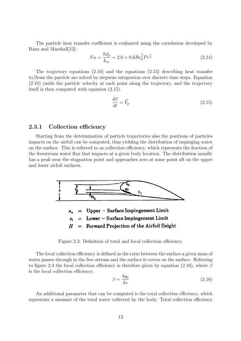
Starting from the determination of particle trajectories also the positions of particlesimpacts on the airfoil can be computed, thus yielding the distribution of impinging wateron the surface. This is referred to as collection efficiency, which represents the fraction ofthe freestream water flux that impacts at a given body location. The distribution usuallyhas a peak near the stagnation point and approaches zero at some point aft on the upperand lower airfoil surfaces.

Figure 2.3: Definition of total and local collection efficiency.

The local collection efficiency is defined as the ratio between the surface a given mass ofwater passes through in the free stream and the surface it covers on the surface. Referringto figure 2.3 the local collection efficiency is therefore given by equation (2.16), where βis the local collection efficiency.

β =δy0

δs(2.16)

An additional parameter that can be computed is the total collection efficiency, whichrepresents a measure of the total water collected by the body. Total collection efficiency

13

is, using the same terminology as in figure2.3, given as:

E =y0

H(2.17)

2.4 Energy and mass balance

The amount of freezing water is computed solving a thermodynamic balance on thesurface of the airfoil. For water to freeze the latent heat of fusion of the droplet mustbe dissipated, through a combination of convective cooling, evaporation and other energyterms that have to be computed. The modelling of icing requires the computation of amass and a thermal balance for each control volume, figure 2.5, located on the surfaceof the body. Initially, the airfoil is divided in a number of segment (figure 2.4), and thelower boundary of the control volume is located on each segment. Therefore, the lowerboundary is initially in contact with the clean surface, and then moves outward with thesurface as ice accretes. The control volume is therefore always either on the clean surfaceor on the iced surface.

Figure 2.4: Identification of the control volumes over each segment defining the body.

From the solution of the thermodynamic balance the freezing fraction can be com-puted, which represent the fraction of liquid water that freezes at each location. If not allof the water freezes, it is assumed that the remaining water (runback water) flows alongthe surface of the body, and it is included in the thermal and mass balance of the succes-sive control volume. The freezing fraction is then used to compute the rate of accretionand the iced geometry at a given time can be determined.

When writing the thermal and mass balance some assumptions have been made:

14

Figure 2.5: Mass balance for each control volume. 1: impinging water; 2: water leaving theairfoil through evaporation or sublimation; 3: runback water leaving the control volume;4: runback water entering the control volume; 5: water leaving the control volume throughicing.

15

• Unfrozen water is only allowed to run back, thus water may not remain on a controlvolume nor be shed.

• Run back is at the freezing temperature of water.

• Radiation is neglected, as it only has limited influence given the low temperaturesinvolved.

• Conduction toward the airfoil is neglected. Heat conduction depends on materialproperty and thickness, and can be accepted considering that it only has limitedinfluence on the ace accretion.

Referring to figure 2.5, the water flux entering the control volume is the sum ofimpinging water and runback water; water can leave the control volume by evapora-tion/sublimation, runback and icing. The mass balance can be written for each controlvolume on the airfoil as:

mimp (i) + mrb in (i) = me (i) + ms (i) + mrb out (i) + mice (i) (2.18)

Where the mass fluxes terms considered are:

• impinging: sum of the mass flow rate of impinging water on the panel.

mimp (i) =∑

mp (2.19)

• runback in: mass flow rate of water flowing into the panel.

mrb in (i) = mrb out (i−1) (2.20)

• evaporation: mass flow rate of water which evaporates.

me (i) = ds Hg

pww

Tsurf− r pedgepw

Tedgepsurfpedge

0.622Tedge− pww

Tsurf

(2.21)

• sublimation: mass flow rate of ice which sublimates.

ms (i) = ds Hg

pwi

Tsurf− r pedgepw

Tedgepsurfpedge

0.622Tedge− pwi

Tsurf

(2.22)

• runback out: mass flow rate of water flowing out of the panel.

mrb out (i) = mimp (i) + mrb in (i) − me (i) − ms (i) − mice (i) (2.23)

16

• icing: mass flow rate of water freezing.

mice (i) = (mimp + mrb in − me − ms)n(i) (2.24)

The mass transfer coefficient in equation (2.21) and (2.22) is defined as:

Hg =Hc

cp

(Pr

Sc

) 23

(2.25)

Pr =cp µ

k(2.26)

Sc =µ

ρ Dv

(2.27)

Beside the energy terms related to mass flow indicated before, other energy transfermodes need to be considered; these are the kinetic energy of impacting particles, convec-tion and aerodynamic heating. Using the same control volume concept to formulate theenergy balance on the icing surface:

qw (i) + qk (i) + qrb in (i) + qa (i) = qe (i) + qs (i) + qrb out (i) + qice (i) + qc (i) (2.28)

Where the energy terms considered, computed considering ice at 0 K as the referencecondition for zero internal energy, are:

• water: energy of impinging water.

qw (i) = mimp (i) [cpice Tf + Lf + cpw (Timpact − Tf )] (2.29)

• kinetic: kinetic energy of water striking the surface.

qk (i) =1

2mimp (i)V

2impact (2.30)

• runback in: energy of water flowing into the panel.

qrb in (i) = mrb in (i) [cpice Tf + Lf ] (2.31)

• aerodynamic: aerodynamic heating of the surface.

qa (i) =ds Hc Vedge

2

2 cp(2.32)

• evaporation: energy of water which evaporates.

qe (i) = me (i) [cpice Tf + Lf + cpw (Tv − Tf ) + Lv + cpv (Tf − Tv)] (2.33)

• sublimation: energy of ice which sublimates.

qs (i) = ms (i) [cpice Tf + Ls + cpv (Tsurf − Tf )] (2.34)

17

• runback out: energy of water flowing out of the panel.

qrb out (i) = mrb out (i) [cpiceTf + Lf ] (2.35)

• icing: energy of ice accumulation.

qice (i) = mice (i) [cpice Tsurf [ (2.36)

• convection: energy lost/gained by convection.

qc (i) = ds(i) Hc (Tsurf − Tedge) (2.37)

The conditions at the edge of the boundary layer are needed to compute some of theterms. These are obtained from the flow solution considering the Mach number constantthrough the boundary layer. Hence:

Medge = Msurf (2.38)

Tedge = T∞

1 +γ − 1

γM2∞

1 +γ − 1

γM2

edge

(2.39)

pedge = p∞

(TedgeT∞

) γ

γ − 1 (2.40)

Vedge = Medge

√γRTedge (2.41)

The energy and mass balance equations are combined to find the local freezing fraction(2.42), that is the ratio of water freezing to water entering the panel.

n(i) =−qw (i) − qk (i) − qa (i) − qrb in (i) + qc (i) + qe (i) + qs (i)

(mimp (i) + mrb in (i) − me (i) − ms (i))(−cpiceTsurf + Lf + cpiceTf )

+(mimp (i) + mrb in (i) − me (i) − ms (i))(cpiceTf + Lf )

(mimp (i) + mrb in (i) − me (i) − ms (i))(−cpiceTsurf + Lf + cpiceTf )(2.42)

Because of its definition, the freezing fraction can not be greater than 1. If the valuecomputed using equation (2.42) is larger it is assumed that n = 1. Again, the freezingfraction can not be negative, therefore if the value computed with (2.42) is non positiveit is set n = 0.

One of the variables in equation (2.42) is still unknown, namely the terms associatedwith runback water. Thus the thermodynamic balance is first solved at stagnation point,where water only enter the control volume through impingement; the mass flux of ice isthen computed using (2.24) and the mass flux of runback leaving the control volume iscomputed using (2.23).

The runback water leaving the stagnation point is then used as an input for panelimmediately downstream; here the mass flux of runback water entering is set equal to thevalue computed with (2.23) for the previous panel. The ice thickness at a given location

18

is then given by equation (2.43), where the density of ice(2.44) is a function of velocity,temperature and particle diameter. Indeed, depending on icing condition the density ofice changes because of the presence of air bubble inside the ice structure.

b(i) =mice (i) ∆t

ds ρice(2.43)

If 1 ≤ −dp V∞2 T∞

≤ 17 and T < −5◦C ρice = 110

(−dp V∞

2 T∞

)0.76

(2.44)

Else ρice = 917 kg/m3 (2.45)

The density of ice in equation (2.44) and (2.45) is based on an empirical relation whichrelates density with external temperature, velocity and particle diameter, and has beenderived in [14].

2.4.1 Ice temperature

When the thickness of ice to be added at each location and its properties are knownthe temperature on iced surface is computed. This is temperature used for the next timestep as a condition on the airfoil. Depending on the freezing fraction, the value of thesurface temperature is computed as follows. If the freezing fraction is less than 1, that isnot all of the water freezes, the surface temperature is set equal to 273.15 K, that is thetemperature of the water film. In case of a rime accretion, that is freezing fraction equalto 1, the surface temperature is computed considering the conduction through the icedlayer, using equation (2.46), assuming the temperature varies linearly in the ice.

Tsurf(t+1) = Tsurf(t) + bqa (i) + qk (i) + qrb in (i) + qwater (i) − qice (i) − qc (i) − qs (i) − qe (i)

kice ds(2.46)

Energy term associated with water freezing is computed with:

qice (i) = n(mimp (i) + mrb in (i) − me (i) − ms (i)

)(cpiceTsurf ) (2.47)

Beside the temperature on the iced surface, also the initial temperature of the airfoilhave to be computed. This is computed at the beginning of the process, solving thethermodynamics balance previously described. It is first assumed that the surface tem-perature is equal to 273.15 K, that is not all water freeze. The terms in equations (2.28)and (2.18) are evaluated using this temperature and a value for the freezing fraction iscomputed. Three cases are then possible:

1. Freezing fraction less than 0.

2. Freezing fraction between 0 and 1.

3. Freezing fraction greater than 1.

If the freezing fraction is between 0 and 1 than water is indeed flowing on the surface,and the guessed value for surface temperature is retained. If the freezing fraction isgreater than 1 than all impinging water is freezing, therefore the surface temperature

19

must be lower than the freezing temperature. The surface temperature is computed bysolving equations (2.28) and (2.18) by imposing n = 1. This is done by applying aniterative procedure, because many terms depend on the surface temperature. In case offreezing fraction below 0 than the surface temperature is greater than 273.15 K; similarly,equations (2.28) and (2.18) are solved imposing n = 0.

20

Chapter 3

Numerical tool: IceMAP 2D

The numerical model presented in the previous chapter has been implemented in thetool IceMAP 2D (Module for Accretion Prediction). With this tool it is possible tosimulate the ice accretion over bi dimensional bodies by means of a CFD software. TheReynolds Averaged Navier-Stokes (RANS) equations and the boundary layer are solvedat predefined grid points locations. Thus, compared with panel method, it provides amore accurate flow field solution, without the limitation of a potential flow solver; indeed,with a CFD software simulations at high Mach number and high angle of attack, as wellas flow separation can properly be solved.

IceMAP 2D has been initially developed so that the simulation of ice accretion could beembedded in Fluent, that is the CFD software used within the aerodynamic departmentof Agusta Westland. Although Fluent is used to determine particle trajectories andcompute collection efficiency, it has not the capability to perform ice accretion simulationThis module has been completely developed; the tool is written in the C language andintegrated using the user-defined functions, which are part of Fluent and designed tointeract with the solution process. Thus, also the solution of the thermodynamic balancehas been integrated within Fluent. This allows to use all the capabilities of the CFD;the flow field and particle tracking are computed by Fluent, but also the variables usedin the solution of thermodynamic balance on the surface are derived directly from theflow field solution, as is the case for the heat transfer coefficient. The need for empiricalrelations, necessary to provide a solution of the boundary layer and a value of heat transfercoefficient, is thus eliminated.

ANSYS R© WorkbenchTM

has been used to integrate in a single application the wholeprocess, creating a loop that includes also the mesh generation and modification (timestepping capabilities). An algorithm has been implemented to manage the process inWorkbench, and eventually it has been fully automated.

IceMAP 2D requires as input flight and icing conditions, together with the airfoilgeometry, while the rest of the process does not require any user intervention, and givesas a result the final ice shape and the aerodynamic coefficients on the iced body.

3.1 Procedure for ice accretion computation

As ice grows on the airfoil, the flow field and the impinged area on the surface changes.Therefore, the total accretion time is divided in a discrete number of smaller time step,

21

and at each step the solution process is repeated. At each time step the ice accretionsimulation is composed of different blocks, that have to be executed sequentially in orderto obtain the final results.

The blocks composing the accretion process are visible in the flow diagram 3.1. Itis first necessary to define all of the input required for the icing simulation, which canbe divided in definition of the geometry of the body and the external conditions; theseinclude the free stream conditions of the flow, like velocity and temperature, and the icingconditions, like particle diameter and number of time steps.

Figure 3.1: Illustration of the solution process with IceMAP 2D.

The geometry of the surface is then used to define the computational domain andthe creation of the proper mesh. Using the input free stream condition the flow fieldsolution is then computed solving the Navier-Stokes equation by means of Fluent; theinitial temperature of the surface and the heat transfer coefficient between the body andthe air can thus be determined. With the correct surface temperature the flow field issolved again, so that the forces acting on the droplets and local aerodynamic field aroundthe body can be computed.

At this point the ice accretion module can be launched, which can be divided in threemajor blocks: particle tracking, solution of the thermodynamic balance and geometry and

22

mesh update. The blocks are visible in 3.2, and have been implemented in Fluent mainlythrough the usage of user defined function. Initially a discrete number of particles aretracked through the fluid domain to determine where and what rate they impact theybody, so that the collection efficiency and impinging mass at each surface location can becomputed.

Figure 3.2: Ice accretion module, implemented in Fluent using user defined functions.

With the data from the particle tracking and the flow solution the thermodynamicbalance is solved on the surface; this allows to determine the fraction of water that freezeson the surface and using the time increment specified by the user also the ice thickness tobe added. The temperature on the iced surface is then computed and used as a boundarycondition for the subsequent flow and thermodynamic solution. The last step of theice accretion module is the geometry and mesh modification to take into account thedeformation due to the ice accumulation.

At the end of each ice accretion module IceMAP 2D checks whether the requestednumber of time steps has been reached; if other time steps are required, the quality ofthe mesh is controlled and recreated if necessary to ensure that it meets certain qualityrequirements before repeating the process. If the required number of time steps has beenreached the aerodynamic coefficients on the iced airfoil are computed.

This iterative process thus can be divided in:

1. Mesh definition.

2. Heat transfer coefficient determination.

3. Flow field simulation.

4. Discrete phase simulation.

5. Thermodynamic balance solution.

23

6. Ice accretion.

7. Mesh check.

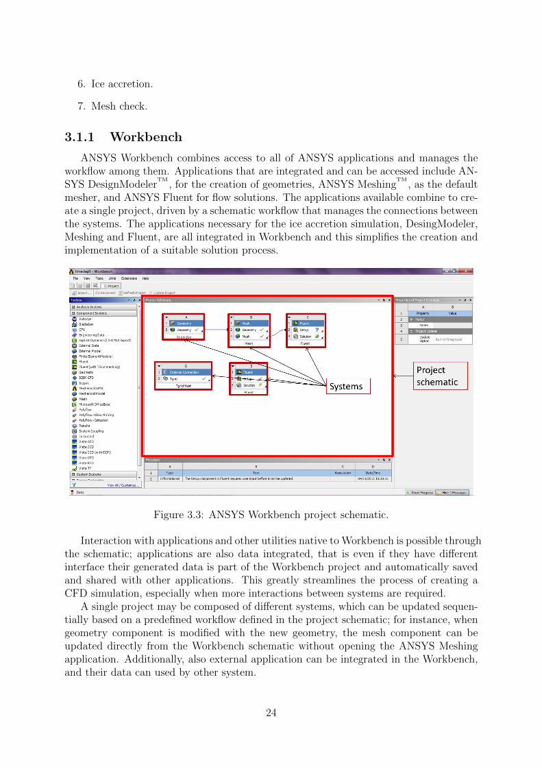
3.1.1 Workbench

ANSYS Workbench combines access to all of ANSYS applications and manages theworkflow among them. Applications that are integrated and can be accessed include AN-SYS DesignModeler

TM, for the creation of geometries, ANSYS Meshing

TM, as the default

mesher, and ANSYS Fluent for flow solutions. The applications available combine to cre-ate a single project, driven by a schematic workflow that manages the connections betweenthe systems. The applications necessary for the ice accretion simulation, DesingModeler,Meshing and Fluent, are all integrated in Workbench and this simplifies the creation andimplementation of a suitable solution process.

Figure 3.3: ANSYS Workbench project schematic.

Interaction with applications and other utilities native to Workbench is possible throughthe schematic; applications are also data integrated, that is even if they have differentinterface their generated data is part of the Workbench project and automatically savedand shared with other applications. This greatly streamlines the process of creating aCFD simulation, especially when more interactions between systems are required.

A single project may be composed of different systems, which can be updated sequen-tially based on a predefined workflow defined in the project schematic; for instance, whengeometry component is modified with the new geometry, the mesh component can beupdated directly from the Workbench schematic without opening the ANSYS Meshingapplication. Additionally, also external application can be integrated in the Workbench,and their data can used by other system.

24

As stated, the process developed for ice accretion simulation involves different steps,which also need to be repeated: geometry and mesh creation, flow solution and ice accre-tion with Fluent, mesh update. The whole process can be included in a single Workbenchproject, which greatly simplify the management of different components required. Anadditional advantage of using Workbench resides in the scripting and journaling capabil-ity, that is the possibility of writing a set of instructions to be executed and record theaction performed via the graphical user interface. Scripts and journal are written in thePython language, and they allow to replay simulations already run as well as to automaterepetitive analyses.

With scripting, it is also possible to interact and launch applications integrated inANSYS Workbench. Although for some applications is not possible to directly modifythe operations executed, it is possible to use their own native scripting language; forexample, operations in DesignModeler, used to create the domain geometry and basedon JavaScript, are not journaled in Workbench, but is possible to launch script from theWorkbench.

All these capabilities make ANSYS Workbench ideally suited to contain an iterativeprocess as an ice accretion simulation is. Further, the process can also be automatizedusing a script written in python language. Using a script all the capabilities of ANSYSWorkbench are available, but without the need to directly interact with any of the systems.Indeed, a single script is responsible of creating the various systems needed, launchingapplications when required and sending the appropriate commands. This completelyeliminates the need of user intervention; a minimal number of input are required, whilethe script manages the whole process until a final ice shape is obtained.

3.1.2 UDF development

A user-defined function is a function written in C that can be loaded in Fluent toenhance its features; using UDF is possible to customize boundary conditions, executeon demand some operations, contained in a UDF, enhance post-processing and modelsexisting in Fluent, such as discrete phase model. User defined function are defined usingmacros supplied by Fluent, and have access to the solver data and may also perform othertasks. Thanks to the UDF feature, that allows the information exchange with the solver,the ice accretion module has been completely integrated in Fluent.

The solution process in Fluent, considering UDFs, for the pressure-based coupledsolver begins with a two steps initialization sequence that is executed outside of the so-lution iteration loop. The solution iteration loop begins with the execution of ADJUSTUDFs, used to adjust or modify Fluent variables (for example velocities or pressure).Next, Fluent solves the governing equations of continuity and momentum in a coupledfashion. Energy, species transport, turbulence, and other transport equations are solvedsequentially, calling UDFs when necessary; finally, a check for either convergence or ad-ditional iterations is done, and the loop either continues or stops.

The ice accretion module is written as a user defined function, executed on demandafter the flow field solution has been obtained. To work properly, it needs additionalUDFs, which are used to initialize local variables, define particles properties, boundaryconditions for the discrete phase model, and to store variables from the particle tracking.

Finally, the update of the mesh based on the iced geometry is also governed by a user

25

Figure 3.4: Solution process of Fluent with UDFs. Image from [3].

defined function, which is called in the mesh morphing process in Fluent to define thenew nodes positions.

26

3.2 Geometry and Mesh

The solution of the flow field is computed considering a C-shaped computational do-main (figure 3.5), with the frontal arc centred on the leading edge of the airfoil. Theoverall size of the domain is defined in number of chords before and after the airfoil, andcan be specified by the user. The domain have to be large enough so that the flow at theboundaries is not altered by the presence of the airfoil.

Figure 3.5: Domain and mesh used. The airfoil is at the centre of the domain.

Fluent solves the given set of equations in a number of discrete points in the domain;the discretization and resolution of the domain influences the accuracy of the solutionas well as the computation cost of the simulation. The volumetric mesh has be builtconsidering two key parameters: the accuracy of the simulation and the computationalcost involved. The accuracy of the flow solution directly impacts the aerodynamic char-acteristics and the parameters computed on the airfoil; therefore, the particle trajectoriesand the solution of the thermodynamic balance on the surface are affected and may resultin a large difference in the computed ice shape. Computational costs are involved bothin the mesh generation process and in the flow solution via CFD. Moreover, because thesimulation is a multi step procedure, at each step the geometry and the mesh have to bemodified if not completely regenerated. This is the result of the complex shapes typicalof ice formation, which may invalidate the mesh generated for the previous time step.Figure 3.6 and 3.7 provide an example of the large difference between the clean and icedairfoil and the mesh differences. Beside the costs due to the mesh generation also theflow solution has to be computed at each time step, which further increase the compu-tational demand. Minimizing the computational costs can thus significantly reduce thetime required to run a simulation.

27

Figure 3.6: Mesh for a clean airfoil NACA0015. Unstructured, triangular mesh.

The volumetric mesh used, as can be seen in figure 3.6, is an unstructured grid made bytriangular elements. The creation of structured mesh, consisting of quadrilateral element,may in case of large ice accretion be extremely difficult and time consuming; additionally,in structured quadrilateral mesh the distribution of cells may be less efficient, because themesh structure forces a fine resolution in areas where it is not required. As a result thecomputational time necessary to generate a structured mesh is elevated and may resultin an unnecessarily high cell count. On the contrary, triangular meshes generally requireless setup time and allows more freedom in the placement of cells, thus allowing clusteringof elements in specified regions of the flow domain. In icing simulation large horns andirregular surfaces may be expected, as can be seen in figure 3.7, and the advantages offeredby triangular mesh are particularly useful.

Generally, increasing the number of elements of the mesh a more accurate flow solutionis obtained, at the expense of the computational time, which is heavily increased by themesh generation and flow solution process. A proper clustering strategy can be employedto significantly reduce the number of cells without deteriorating the accuracy of the flowsolution. The element size is variable on the domain, so that the cells are larger farfrom the airfoil, where the flow is slightly influenced by the presence of the airfoil; onthe contrary, near the airfoil the size of cells is dramatically reduced, so that smaller flowcharacteristic can be distinguished.

To better model the boundary layer the mesh should be particularly refined near thewall; a characteristic of quadrilateral cells is that they permit a larger aspect ratio (thatis base length to height ratio) than triangular cells, because for the latter it also impactthe skewness and may impede the accuracy and convergence of solution. In the case ofthe boundary layer, though, it can be modelled using some layers of quadrilateral cells onthe surface of the airfoil. In the boundary layer the flow is aligned with the airfoil, andthe length of the cells does not affect the accuracy of the solution.

28

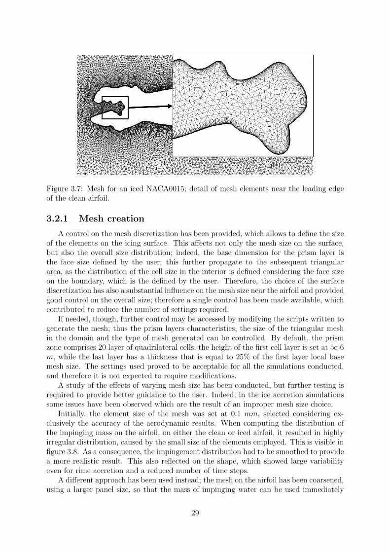
Figure 3.7: Mesh for an iced NACA0015; detail of mesh elements near the leading edgeof the clean airfoil.

3.2.1 Mesh creation

A control on the mesh discretization has been provided, which allows to define the sizeof the elements on the icing surface. This affects not only the mesh size on the surface,but also the overall size distribution; indeed, the base dimension for the prism layer isthe face size defined by the user; this further propagate to the subsequent triangulararea, as the distribution of the cell size in the interior is defined considering the face sizeon the boundary, which is the defined by the user. Therefore, the choice of the surfacediscretization has also a substantial influence on the mesh size near the airfoil and providedgood control on the overall size; therefore a single control has been made available, whichcontributed to reduce the number of settings required.

If needed, though, further control may be accessed by modifying the scripts written togenerate the mesh; thus the prism layers characteristics, the size of the triangular meshin the domain and the type of mesh generated can be controlled. By default, the prismzone comprises 20 layer of quadrilateral cells; the height of the first cell layer is set at 5e-6m, while the last layer has a thickness that is equal to 25% of the first layer local basemesh size. The settings used proved to be acceptable for all the simulations conducted,and therefore it is not expected to require modifications.

A study of the effects of varying mesh size has been conducted, but further testing isrequired to provide better guidance to the user. Indeed, in the ice accretion simulationssome issues have been observed which are the result of an improper mesh size choice.

Initially, the element size of the mesh was set at 0.1 mm, selected considering ex-clusively the accuracy of the aerodynamic results. When computing the distribution ofthe impinging mass on the airfoil, on either the clean or iced airfoil, it resulted in highlyirregular distribution, caused by the small size of the elements employed. This is visible infigure 3.8. As a consequence, the impingement distribution had to be smoothed to providea more realistic result. This also reflected on the shape, which showed large variabilityeven for rime accretion and a reduced number of time steps.

A different approach has been used instead; the mesh on the airfoil has been coarsened,using a larger panel size, so that the mass of impinging water can be used immediately

29

Figure 3.8: Impinging water on clean and iced airfoil, element size 0.1 mm, no smoothing.

Figure 3.9: Impinging water on a clean NACA0012 airfoil, mesh size 0.1 mm and 2 mm.

30

Figure 3.10: Ice shape with mesh size of 0.1 mm and 2 mm.

in the computation of the iced characteristics. The difference in the computed impingingmass with element size of 0.1 mm and 2 mm is visible in figure 3.9; in the finer meshsize the impinging mass was smoothed, but still presented some irregularities. In figure3.10 also the final ice shape is computed, using two time steps for the finer mesh andfive for the coarse mesh. Although ice accretions are not smooth, the irregularities visibleusing the finer mesh can not be considered representative, because they are the results ofthe numerical inaccuracies in the impinging mass, visible in figure 3.9. Additionally, thenumber of time steps usable was dictated by the difficulties encountered in the generationof the mesh for iced surface, because it often resulted in invalid cells near the surface. Theissues noted for the finer mesh are largely eliminated considering coarser mesh element.

Some tests have also been conducted by further increasing the size of the surfaceelements; these resulted in an excessive simplification of the geometry, thus the final iceaccretion may be missing relevant ice features like horns. In figure 3.11 the simplificationscaused by the excessive size of the mesh are clearly visible.

The external conditions are the same in both cases, and are representative of a pro-longed (22.5 minutes) glaze accretion a GLC305 airfoil with a 0.91 m chord length. Whenthe coarser mesh is used, the final ice shape only has limited resemblance to the ex-perimental shape, as the horns are completely missing. Halving the mesh size largelyimproves the result, and in the final accretion also the presence of horns is visible. In thiscase the difference is especially clear, as the airfoil used is particularly thin; the maximumthickness of the airfoil is indeed of only 7 cm, for which a 4 mm element size representsa considerable part of the leading edge section. In this specific case no tests have beenconducted using smaller mesh size, but may further improve the results.

For the cases considered the size of the mesh is generally around 1 mm, with somevariability due to the overall length and thickness of the airfoil simulated; for smallerobjects, like a 0.15 m NACA0012, a 0.5 mm has been used without adverse effects.

Based on the tests executed, the user should use a mesh size between 0.5 and 2 mm,

31

Figure 3.11: Effect of mesh size on ice accretion. Mesh size: 2 mm left, 4 mm right.

which has been found appropriate for most simulations; the choice should be based prin-cipally on the thickness of the specific airfoil, and in second instance on the chord length.Although no comprehensive series of tests on the effect of mesh size on ice accretion hasbeen conducted, the 2 millimetres used in the previous example can be safely consideredas an upper limit that should not be exceeded, unless for particularly long and thickobject. In some cases also smaller elements may be appropriate, but numerical problemsmay arise.

Figure 3.12: Detail of the mesh used for ice accretion. Element size 2 mm.

The mesh size previously indicated is used in the computation of the ice growth andgenerally provides satisfactory results in the computation of the aerodynamic characteris-tics of the airfoil. To ensure that the flow over the surface is properly modelled, a different

32

Figure 3.13: Detail of the mesh used for aerodynamic purpose. Element size 0.1 mm.

mesh size may be specified for the determination of the aerodynamic characteristics of thefinal ice shape. An example of the different refinement in the mesh used in the accretionprocess and the final computation of the aerodynamic characteristic is shown in figure3.12 and 3.13. The element size for the aerodynamic mesh is set by default at 1e-4 m, asin 3.13, which guarantees adequate modelling of the flow under all the conditions testedand that may be expected.

A different value may be used, which should be dictated only by aerodynamic consid-erations, as the negative effects noted in the ice accretion process are not present here.As a consequence of the finer mesh also the aerodynamic coefficients computed shouldbe more representative of the actual values compared to those computed with a coarsermesh. The computational cost of the simulation is also increased, but can be acceptedconsidering that the mesh is only used for a single flow solution.

3.2.2 Mesh refinement

The default mesher in Workbench is ANSYS Meshing, which is integrated with theother applications used. Therefore, the iced geometry could be automatically importedin the meshing tools, and similarly the generated mesh was imported in Fluent withoutintervention.

Despite the inherent advantages of using ANSYS Meshing, it has been found that inmany circumstances can not generate the desired mesh. Therefore, in some cases therepresentation of the boundary layer using the prism cells is completely missing, or thecells created are highly skewed; this occurs especially in the case of glaze accretion, nearhorns or irregular shapes. As a result, it is not possible to compute an accurate solutionof the flow in Fluent. A unique solution that can provide an acceptable mesh, with allthe characteristics required, for the possible ice shape, thus including glaze accretion, hasnot been found.

33

Figure 3.14: Tgrid in the project schematic of ANSYS Workbench.

Because of the issues encountered, ANSYS Meshing is only used to generate a dis-cretization of the boundaries of the domain, which is then imported in an external mesher,Tgrid

TM, which is widely used in AgustaWestland, including for the generation of meshes

on iced airfoil. To maintain the process in the framework provided by ANSYS Workbench,Tgrid has been integrated using the External Application system.

Figure 3.15: Mesh near horns, Tgrid top and ANSYS Meshing bottom.

With Tgrid it is possible to obtain the meshes as intended, even in the case of glazeice accretion. Additionally, the meshing process in Tgrid can be more easily scripted andmodified if need arise. On the contrary, ANSYS Meshing lack any kind of documentationthat could help the scripting process.

34

Figure 3.16: Mesh on iced airfoil, Tgrid top and ANSYS Meshing bottom.

Image 3.15 shows the same geometry meshed with ANSYS Meshing (bottom) andTgrid (top); here a glaze accretion has produced two horns close to each other, andANSYS Meshing produces some highly skewed cells outside the boundary layer (circledin red). Because of their presence, the convergence of the solution in Fluent is impeded.The top of figure 3.15 shows the same area meshed by Tgrid using the same parametersfor mesh size and no skewed cells are present.

In figure 3.16 an irregular accretion on the iced surface is visible; in this case ANSYSMeshing (bottom) fails to generate the layer of prisms representing the boundary layer.As a result, even if Fluent provides a solution, it is not accurate because the modelling ofthe boundary layer is completely missing. Also in this case Tgrid manages to generate amesh with the layers of quadrilateral cells on the iced surface.

35

3.3 Heat Transfer Coefficient

Heat transfer coefficient is an important variable in the simulation of ice accretion.This can be clearly seen in image 3.18: two runs with the same icing conditions havebeen performed, but the heat transfer coefficient has been computed using a differentturbulence models and surface roughness. The computed heat transfer coefficient in thetwo cases is shown in figure 3.17, while the final ice shape, obtained with the differentvalues of heat transfer coefficient, is given in figure 3.18. The variability of ice shape isthe result of the many terms in the energy balance (equation (2.28)) that depend on heattransfer coefficient, like convective and evaporative cooling. These terms are responsiblefor the freezing of water, thus at lower values of heat transfer coefficient will corresponda decrease in ice formation.

Figure 3.17: Heat transfer coefficient computed with different roughness and turbulencemodel.

Figure 3.18: Ice accretion with different heat transfer coefficient.

The heat transfer coefficient is significantly increased by the roughness of the icedsurface, and in Fluent also by the turbulence model employed. Thus it is essential todetermine how to compute surface roughness to properly simulate the roughness of the

36

iced surface and which turbulence model is the most suited to estimate heat transfercoefficient. Moreover, it has been found that changing the settings for thermal boundarycondition on the airfoil influence the computed heat transfer coefficient.

3.3.1 Effect of surface roughness

Clean aerodynamic surface can be considered smooth, but the growth of ice leads tothe development of surface roughness; the transition to turbulent flow is caused primarilyby the increase in surface roughness, which decides the location of laminar/turbulent tran-sition. The surface roughness therefore enhance the heat transfer coefficient by increasingthe effective area on the airfoil and increasing the skin friction coefficient. Experimentalstudies[16] show that roughness is higher for glaze accretion, while is relatively moderatefor rime ice.

In report [12] the local heat transfer coefficients for a smooth and roughened NACA0012 were measured in flight at different angles of attack. Roughness was simulatedattaching hemispheres of 2 mm diameter on the surface of the airfoil on a predefinedpattern.

The heat transfer coefficient measured in [12] for a smooth and a roughened airfoilare shown in figure 3.21 and 3.22, while the distribution of the roughness element on thesurface is visible in figure 3.19 and 3.20.

Figure 3.19: Dense roughness pattern on airfoil. Location identified by the number, with1 = -0.036 s/c and 12 = 0.095 s/c. Heat transfer coefficient measured at 0◦ and 4◦.

Figure 3.20: Sparse roughness pattern on airfoil. Location identified by the number, with1 = -0.036 s/c and 12 = 0.095 s/c. Heat transfer coefficient measured at 0◦.

37

Figure 3.21: Heat transfer coefficient measured in flight for smooth and roughened NACA0012, angle of attack 0 ◦. Two roughness pattern used. Data from [12].

Figure 3.22: Heat transfer coefficient measured in flight for smooth and roughened NACA0012, angle of attack 4 ◦. Data from [12].

38

The data were obtained at an angle of attack of 0 and 4 degrees. The dense patternwas used for both angles of attack, while results for the sparse pattern are only shown for0 degrees angle of attack. In both cases the heat transfer coefficient for the roughenedairfoil is larger than for the smooth airfoil, especially downstream of the stagnation. Thedifference increases when the density of roughness element increases, as the boundarylayer is more and more influenced by the roughness. The variation of the heat transfercoefficient at some location is extremely large, with values more than doubling over theircorresponding smooth value. This is even more dramatic increasing the the angle ofattack, where the measured heat transfer coefficient is at some point more than fourtimes larger than the smooth value.

A similar effect can be observed in Fluent and is visible in figure 3.23, where the heattransfer coefficient is computed for a smooth and roughened surface under the same ex-ternal conditions. The value is similar at the stagnation point, but further aft on eitherthe upper or the lower airfoil surface the difference becomes significant and results indrastically different ice shape. Because of the lower heat transfer coefficient less waterfreezes immediately and flows on the surface, eventually freezing at some location down-stream. Therefore, the ice thickness at the stagnation is reduced, while ice grows pastthe experimental accretion limits. This is clearly visible in figure 3.24 and 3.25, whichrepresents a three minutes glaze ice accretion on a NACA 0012 airfoil. The only differencein the simulation process is the inclusion of the surface roughness in 3.25; the modifiedheat transfer coefficient is visible in figure 3.23. Although this is a short simulation theice shapes are already quite different, and it is expected to become more significant forlonger accretion time.

Figure 3.23: Heat transfer coefficient for a smooth and rough NACA 0012; the final iceshape with the different values of htc is visible in figure 3.24 and 3.25.

Because of the large variation of heat transfer coefficient with surface roughness, andits influence on the ice accretion, it is necessary to model the roughness, also consideringits variability with icing conditions and the type of ice growing.

The lack of detailed informations on how roughness varies with icing conditions haslead to the development of empirical correlations to calculate an equivalent sand grain

39

x/c-0.04 -0.02 0 0.02 0.04 0.06 0.08 0.1 0.12 0.14

y/c

-0.04

-0.02

0

0.02

0.04

0.06

0.08CleanExperimentalLEWICEIceMAP 2D

Figure 3.24: With surface roughness.

x/c0 0.05 0.1 0.15 0.2

y/c

-0.06

-0.04

-0.02

0

0.02

0.04

0.06

0.08

0.1CleanExperimentalLEWICEIceMAP 2D

Figure 3.25: Without surface roughness.

40

surface roughness, which do not take into account the physics of ice accretion or theactual conditions of the iced surface. Instead, they are based on the selection of thesurface roughness that best fits the experimental ice shapes.

Figure 3.26: Illustration of the equivalent sand grain roughness concept employed inFluent.

Surface roughness is computed using a correlation presented in [14] and developed bythe author. Ruff correlation given in (3.1) uses external conditions (velocity, temperatureand liquid water content) to estimate the average surface roughness on the iced surface.The correlation is based on experimental data presented in [1].

ks = ksV∞ ksLWC ksT 0.00117 chord (3.1)

ksV∞ = 0.4286 + 0.0044139V∞

ksLWC = 0.5714 + 0.2457LWC + 1.2571LWC2

ksT = 46.8384

(T∞

1000

)− 11.2037

In equation (3.1) the velocity is in m/s, the LWC in g/m3 and the temperature in K.These three icing parameters were selected because of their influence on the type of icegrowing, and because a complete set of experimental data existed from which to form acorrelation. The model has some limitations, due to the fact that it does not take intoaccount the physics of ice accretion, especially for glaze condition, when a water filmcovers the iced surface. For this reason improving the surface roughness model couldimprove the final ice shape, especially in glaze condition.

In Fluent the equivalent sand grain surface roughness computed using equation (3.1) isthen specified in the boundary conditions for the airfoil, so that the fluid flow is computedconsidering a rough surface.

3.3.2 Effect of turbulence model

The heat transfer coefficient is largely influenced by the boundary layer on the airfoiland therefore its modelling has a significant impact on the computed heat transfer. InFluent many different formulation for turbulence are available, but it has been foundthat not all of them provide accurate results for the heat transfer coefficient. As anexample, figure 3.28 and 3.29 show a three minutes glaze accretion over a NACA0012airfoil, where the heat transfer coefficient, shown in figure 3.27, is computed using thekε − realizable turbulence model and the SST model. The heat transfer coefficientcomputed with the SST model is significantly lower than in the case of the kε−realizable,especially at the leading edge. This has a dramatic consequence on the final ice shape,because the convective and evaporative cooling are minimal; therefore, less water freezes

41

and flows further back and consequently the icing limits are overestimated. The effect islikely to become even more evident at increasing accretion time, therefore ensuring thatthe turbulence model employed to compute the heat transfer coefficient is accurate isextremely important.

Figure 3.27: Heat transfer coefficient computed with kε− realizable and SST model.

The accuracy of the turbulence models has been verified with flight and experimentaldata for a NACA 0012 airfoil, available in a report by NASA[12]. In the paper theFrossling number, computed with equation (3.2), was used to compare the heat transfercoefficient, and therefore it has also been computed in Fluent for uniformity.

Fr =Nu

Re0.5 =

Hc c

kρ V∞µ

0.5 (3.2)

In figure 3.30 the Frossling number for a smooth NACA0012 airfoil, computed in flightand in wind tunnel, is compared with Fluent, using the kω − SST and SST turbulencemodel. Although both models show good agreement, the Frossling number computedwith the SST model is more accurate especially further away from the leading edge.

Beside the results for a smooth NACA 0012, in [12] also measurement for a roughenedairfoil were presented. The surface roughness was simulated with hemispheres placed onthe surface of the airfoil, an example of which is visible in figure 3.20 and 3.19. Because ofthe good agreement between SST and experimental data, it was expected that it wouldstill provide accurate result when including the effect of roughness. Unfortunately, ithas been found that the SST model largely under predicts the value of heat transfercoefficient at the leading edge. This is visible in figure 3.31, where the surface roughnesswas simulated using the pattern in figure 3.19. The kε− realizable and SST models arecompared with experimental data, obtained at the Icing Research Tunnel, and an integralboundary layer solution, similar to what is used in LEWICE.

A value of 0.000573 m for the surface roughness was used in the integral boundarylayer solution from the correlations given in (3.1), considering a velocity of 62 m/s, statictemperature of 266 K and liquid water content of 0.5 g/m3, assumed as a default value. In

42

x/c-0.04 -0.02 0 0.02 0.04 0.06 0.08 0.1 0.12 0.14

y/c

-0.04

-0.02

0

0.02

0.04

0.06

0.08CleanExperimentalLEWICEIceMAP 2D

Figure 3.28: kε− realizable turbulence model used to compute heat transfer coefficient.

x/c0 0.05 0.1 0.15

y/c

-0.06

-0.04

-0.02

0

0.02

0.04

0.06

0.08

0.1 CleanExperimentalLEWICEIceMAP 2D

Figure 3.29: SST turbulence model used to compute heat transfer coefficient.

43

Figure 3.30: Frossling number for a smooth airfoil, flight and wind tunnel data comparedwith Fluent. Reynolds number approximately 1280000.

Figure 3.31: Icing Research Tunnel data compared with Fluent and integral boundarylayer solution.

44

Schlicting[15][2] the concept of equivalent sand grain roughness was used to characterizeother types of pattern, which are similar to those used in [12]; using this correlation a valueof 0.000305 m for the equivalent sand grain roughness can be estimated, and was also usedin an integral boundary layer solution. The Frossling number using both roughness valueis visible in figure 3.31. In Fluent a single value for the surface roughness has been used,to test the differences between turbulence model. The sand grain roughness was set at0.000452 m, as is close to the mean values used in the integral boundary layer solutions.

The integral boundary layer solution does not provide a good match of experimentaldata, especially in the area near the leading edge, where the heat transfer is widelyoverpredicted. The turbulence models used in Fluent, especially the kε − realizable,yields more accurate results overall. Both the kε−realizable and the SST provide valuescomparable with experimental data further from the leading edge (s/c > 0.03); in thearea near the leading edge the difference is larger, especially for the SST model, whichlargely under predicts the Frossling number, while for kε − realizable is fairly close tothe experimental values. Both Fluent turbulence models fare well in comparison withthe integral boundary layer solution, as they both provide a more accurate heat transfercoefficient throughout.

However, it must be noted the roughness pattern employed in [12] are not exactly thesame used by Schlicting, therefore the equivalent sand grain roughness value 0.000305 maybe treated as an estimate. Additionally, the roughness correlation (3.1) was derived fromexperimental ice shapes and therefore may not yield accurate values for the roughnessused in [12].

Indeed, the roughness pattern, modelled with hemispherical elements placed on thesurface, does not accurately represent ice roughness, and therefore the differences mayreside in a different modelling; thus the data in [12] may not be used to validate anintegral boundary layer solution based on the surface roughness, as in LEWICE.

LEWICE models the heat transfer coefficient considering the effect of surface rough-ness, and based on the computed value of roughness determine whether the boundarylayer is laminar or turbulent. The heat transfer coefficient computed in LEWICE has alsobeen subject to some validation[14]. The results of the integral boundary layer solutionwere compared with experimental data on a roughened cylinder at various Reynolds num-ber and on simulated ice accretion. The cases tested showed that the predicted valuesof heat transfer coefficient generally compared well with experiments in the leading edgeregion where much of the accretion process takes place.

Therefore the heat transfer coefficient computed in Fluent by different turbulencemodels has also been compared with LEWICE, which is considered to provide accuratevalues of heat transfer coefficient and ice shape.

A comparison is shown in figure 3.32, using for both LEWICE and Fluent the samesurface roughness. The turbulence models used are kω− SST , kε− realizable and SST .

The heat transfer coefficient computed by different turbulence model in Fluent arealmost identical far from the leading edge, and the result can probably be consideredaccurate; indeed, also in the wind tunnel the integral boundary layer solution over pre-dicted the Frossling number far from the leading edge, in an area where no roughnesselements were present, while values computed in Fluent were relatively close. At theleading edge, instead, the difference is larger, with the kε− realizable computing a heattransfer coefficient similar to LEWICE and the other turbulence models under predicting

45

Figure 3.32: Heat transfer coefficient computed with different turbulence model and com-pared with LEWICE.

it.A similar trend is also visible when comparing Fluent with wind tunnel data, where

kε−realizable shows generally better agreement with experimental near the leading edge.Because most of the ice accrues in the leading edge region a proper modelling of the heattransfer coefficient in that area is necessary. Therefore the kε − realizable was used tocompute the heat transfer coefficient, which is subsequently utilized in the solution of thethermodynamic balance.

3.3.3 Thermal boundary conditions

Ideally, the heat transfer coefficient would be computed setting as a boundary condi-tion on the airfoil the appropriate surface temperature. In Fluent, though, it results in thecomputation of unrealistic values when the surface temperature is close to the externaltemperature, as in figure 3.33, where the surface temperature is given in 3.34. In this testcase the free stream temperature was 254.15 K (total temperature ≈ 256 K).

As can be seen the heat transfer coefficient has some peaks where the surface temper-ature reaches a minimum, and then remains negative for the rest of the airfoil. This willresult in a heat flux from the colder surface to the warmer surface, which violates the prin-ciples of thermodynamics, and therefore must be considered the result of computationalerrors in Fluent. Fluent computes the heat transfer coefficient for each wall face using theconvective heat flux at the boundary and the surface and free stream temperature usingequation (3.3). The heat flux is computed by Fluent in the solution process, while thesurface temperature is equal to the temperature of the airfoil.

Hc =qc

Tsurf − T∞(3.3)

Numerical errors may be the result of surface temperature close to the free stream tem-perature, as the denominator approaches zero. This is not acceptable, because the value

46

Figure 3.33: Heat transfer coefficient computed with fixed surface temperature and correcttemperature distribution. Free stream temperature 254.15 K.

Figure 3.34: Temperature distribution on the surface of the airfoil. Free stream temper-ature 254.15 K.

47

of heat transfer coefficient is needed independently of the surface temperature to com-pute the heat fluxes to and from the airfoil; therefore the thermal boundary conditionsin Fluent must be set up so that a realistic value for the heat transfer coefficient is com-puted. The heat transfer coefficient depends on the geometry of the airfoil, the physicalproperties of the fluid, and the characteristics of the fluid flow; although the fluid flowis influenced by the energy flux, it may be neglected if the boundary conditions appliedon the surface are not significantly different from the actual surface temperature. Thusthe effects of varying the thermal boundary conditions have been investigated, so that aboundary condition resulting in an acceptable heat transfer coefficient could be selectedand used in all cases.

The boundary conditions tested are a fixed heat flux and a fixed temperature onthe surface. Different values of heat flux and temperature have been used to verify therepeatability of the data obtained. Because in Fluent the heat transfer coefficient is aderived quantity, a heat flux must always be present, otherwise also the heat transfercoefficient in zero. Therefore the airfoil can not be considered adiabatic.

Figure from 3.35 to 3.39 compare the heat transfer coefficient computed using differentboundary conditions on a NACA 0012 airfoil at 67.1 m/s, freestream temperature of262.15 K and at different angles of attack. In figure 3.35 and 3.36 a fixed heat flux isapplied on the surface to compute the heat transfer coefficient; at zero angle of attackalso the heat transfer coefficient from LEWICE is plotted. Clearly, using too low a heatflux (1000 W/(m2K)) does not reproduce correctly the trend visible in LEWICE, whileincreasing the heat flux results in more consistent result, also comparable with LEWICE.When the angle of attack is set at 4 degrees, the lower heat flux again under estimatesthe heat transfer coefficient when compared with the other heat fluxes applied. Withrespect to the case at 0 degree, a larger variability exists in the coefficient between the10000 and 50000 W/(m2K) heat fluxes, but results are still comparable; additionally, thevariability is mostly far from the leading edge, which is the area more subject to icing. Itmust also be noted that imposing too high a heat flux results in a significant raise in thetemperature on the surface of the airfoil, which may exceed 300 K (figure 3.37); therefore,also the effect of the temperature on the heat transfer coefficient may not be negligible,and caution must be exerted in order to prevent it. On the opposite, small heat flux arenot sufficient to compute accurately the heat transfer coefficient and therefore can notbe considered. The heat flux applied therefore should be in a limited range, so that anaccurate coefficient can be computed without altering the flow near the airfoil.

In figure 3.38 and 3.39 a fixed temperature is used instead as a boundary conditionon the airfoil. The values used are 273.15 and 283.15 K; the lower value is equal to thetemperature of the water film on the surface, and in case of icing at temperature close tofreezing it may be close to the free stream temperature; as a consequence the problemspreviously discussed may still occur. Therefore a second higher value (283.15 K) hasbeen used to verify the results; because no icing occur at temperature that high it shouldnot be encountered in icing simulation and should prevent the denominator of (3.3) frombecoming zero.

At zero angle of attack the heat transfer coefficient is comparable with LEWICE inboth cases and with the fixed heat flux boundary condition. Also at the higher angle ofattack there is good agreement between the two boundary conditions, with less variabilitycompared with the fixed heat flux. Indeed, compared with the fixed heat flux condition

48

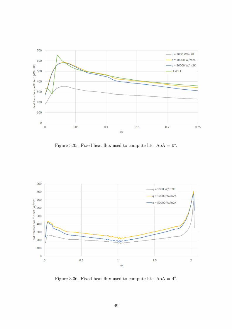
Figure 3.35: Fixed heat flux used to compute htc, AoA = 0◦.

Figure 3.36: Fixed heat flux used to compute htc, AoA = 4◦.

49

Figure 3.37: Surface temperature near the leading of a NACA 0012 airfoil; heat flux 50000W/(m2K), AoA = 0 ◦.

the heat transfer coefficient is less influenced by the difference in the surface temperature.

Figure 3.38: Fixed surface temperature used to compute htc, AoA = 0◦.

When using a fixed heat flux as a boundary condition the surface temperature canstill be expected to be higher that in the case of fixed temperature; additionally, a largervariability can be expected, because the influence on the boundary layer due to the surfacetemperature is higher. Therefore the heat transfer coefficient is computed using a fixedtemperature of 283.15 K as a condition on the surface. In figure 3.40 the heat transfercoefficient is computed at the same external condition as in 3.38, except that the freestream temperature has been increased to 270 K from its previous value of 262.15 K.Therefore also the heat transfer coefficient should not be altered significantly, and the

50

Figure 3.39: Fixed surface temperature used to compute htc, AoA = 4◦.

values computed in LEWICE can still be considered accurate. This is also verified im-posing the higher surface temperature, as the heat transfer coefficient is almost identicalin figure 3.40 and 3.38; on the contrary, using the lower surface temperature (273.15 K)as a boundary condition the computed value is almost half of its original value, that canonly be explained considering the effect of numerical errors.

51

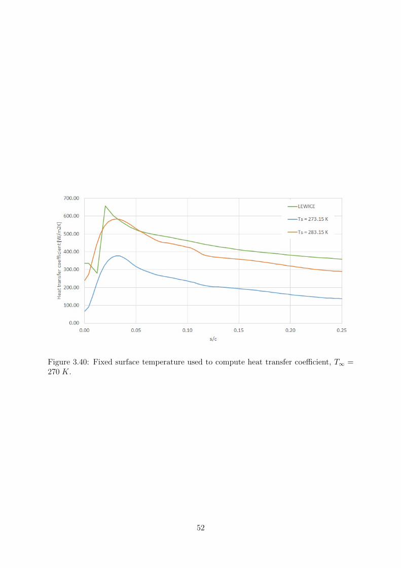
Figure 3.40: Fixed surface temperature used to compute heat transfer coefficient, T∞ =270 K.

52

3.4 Flow field computation

The fluid flow in the domain is solved in Fluent at every time step, considering theboundary conditions applied and the settings used. The boundary conditions specifythe flow and thermal variables on the boundaries of the model, thus they are a criticalcomponent of the simulation.

The pressure far field condition is used in Fluent to model a free stream conditionat infinity, and is used for the external boundary of the domain. The free stream Machnumber, static temperature and pressure and flow direction are specified, considering theambient condition specified by the user.

Figure 3.41: Example of pressure far field settings in Fluent.

The wall boundary condition is used to define the fluid/solid interface, thus is appliedfor the airfoil. The surface temperature, as defined in 2.4.1, and the equivalent sand grainroughness, computed with (3.1), are set for the airfoil. Additionally, the velocity on theairfoil is automatically set to zero for viscous flow to enforce the no-slip condition.

Figure 3.42: Pressure field around a 22.5 minutes ice shape on the Twin Otter tail; angleof attack 0◦, free stream velocity 90 m/s, pressure 97216 Pa.

53

Compressibility effects are encountered in flows at high velocity and in area of largepressure variation. In the case of ice accretion large pressure gradient may be encountered,and the variation of gas density may have a significant impact on the flow velocity andtemperature. Additionally, compressibility effects are also important at high Mach, thusthe compressibility effect have been included to ensure a larger range of validity for theflow solution. Therefore, air is considered an ideal gas and its density at a given locationis computed according to equation (3.4).

ρ =pop + p

R T(3.4)

The viscosity of the fluid under consideration also has an impact on the heat transfer;therefore, the viscosity of the air is considered as a function of temperature and modelledusing Sutherland’s viscosity law, which resulted from a kinetic theory by Sutherland usingan idealized intermolecular-force potential. Sutherland’s law with three coefficients hasthe following form:

µ = µref

(T

Tref

) 32 Tref + S

T + S(3.5)

Where the reference conditions are:

µref = 1.716 · 10−5 (3.6)

Tref = 273.11 (3.7)

S = 110.56 (3.8)

The fluid flow is then solved using the kω − SST (Shear Stress Transport) equation,based on the Reynolds Averaged Equations, which is one of the most widely used modelsfor aerodynamic flows. Compared to kε the kω models are typically better in predictingadverse pressure gradient boundary layer flows and separation. The downside is a strongsensitivity of the solution depending on the free stream values of turbulence. The kω−SSThas been designed to avoid the free stream sensitivity of the standard kω, by combiningelements of kω with kε model; boundary layer is modelled as in kω, while in the far fieldregion, where kω is most sensible to turbulence, like the kε.

Figure 3.43: Velocity flow field around a 22.5 minutes ice shape on the Twin Otter tail;angle of attack 0◦, free stream velocity 90 m/s, pressure 97216 Pa.

The accuracy of the model and the mesh used in the ice accretion process has beentested by comparing the pressure coefficient on the surface with experimental and analyti-cal data for both clean iced airfoil. The data used to verify the Fluent solution is available

54

in [11], and has been obtained at different wind tunnel and using LEWICE potential flowsolution.

A clean GLC 305 and a clean and simulated ice shape on an aircraft (Twin Otter) tailhave been used. Figure 3.46 shows the result for the clean GLC305. In figure 3.44 and3.45 the coefficient of pressure is computed for clean and a 22.5 minutes ice accretion onthe horizontal tail section of the Twin Otter. In all of cases the Fluent solution providesexcellent agreement with experimental data, including for the iced airfoil.

Figure 3.44: Coefficient of pressure on the Twin Otter horizontal tail; angle of attack 0◦,free stream velocity 78.23 m/s, pressure 99974 Pa.

55

Figure 3.45: Coefficient of pressure on a simulated 22.5 minutes ice shape on the TwinOtter horizontal tail; angle of attack 0◦, free stream velocity 90 m/s, pressure 97216 Pa.

Figure 3.46: Coefficient of pressure on a clean GLC 305 airfoil; angle of attack 1.5◦, freestream velocity 78.23 m/s, pressure 98732 Pa.

56

3.5 Particle tracking

The purpose of the discrete phase model is to determine the distribution of impingingwater on the airfoil and to compute the variables associated with impinging particlesnecessary to compute the growth of ice on the surface. In Fluent a second phase, composedof spherical droplets dispersed in the air, can be simulated in a Lagrangian frame ofreference activating the Discrete Phase Model available. Fluent computes the trajectoriesof particles as well as the heat and momentum exchange with the continuous phase, thataffect both the particles and the surrounding air. Because the influence of droplets onthe airflow is marginal, an aerodynamic solution is first computed, and then particletrajectories are simulated. The trajectories and heat and momentum transfer calculationare based on the force balance and the convective heat transfer, defined in section 2.3,using the local conditions of the continuous phase.

3.5.1 Particle initialization

The number of water particles that should be tracked at each iteration can be com-puted from the mean volume diameter and the liquid water content. This is given byequation (3.9), in which the liquid water content is divided by the mass of a single parti-cle.

np =6LWC

πMVD3ρp(3.9)

With a droplets size of 20 µm and a liquid water content of 0.5 g/m3 the number ofparticles in a cubic metre of air is close to 400 millions. This is a prohibitive number ofparticle to be tracked, and therefore in Fluent a number of parcels, each representativeof a fraction of the total mass flow rate, is tracked. A parcel can still be considered asrepresentative of a single particle, as it has the specified diameter and specified propertiesof a single droplet. However, the effect on the continuous phase are computed by summingthe effect of all the particles represented by the parcel.

Therefore, the particles are simulated launching a group of particles in the domain,for which is necessary to define the initial conditions. With these conditions, along withphysical properties defined choosing an appropriate material, the computations of thetrajectories and energy/mass transfer can be initiated. The inputs required are:

• Material.

• Position.

• Velocity.

• Temperature.

• Diameter.

• Flow rate.

Selecting as material liquid water the physical properties necessary to compute the particletrajectory and heat transfer are automatically defined. The initial position must be farenough from the airfoil that the flow is not influenced by the airfoil, and is required as

57

Figure 3.47: List of particle properties. These are set using a UDF.

an user input. The particles velocity and temperature are set equal to the velocity ofair at the same location, as computed by Fluent solving the continuous phase. Indeed,when particles are far from the airfoil, they can be considered in equilibrium with thecontinuous phase, and hence the settings used are appropriate. The diameter is constantand equal to the median volumetric diameter of the icing conditions. Finally the massflow rate associated with each parcel is computed using the local air velocity and liquidwater content, using equation (3.10); additionally, the launch coordinates and the numberof parcels is used.

m = (LWC)Vymax − ymin

np

(3.10)

The inputs are automatically computed in a user defined function, which is responsibleof defining the appropriate variables.

3.5.2 Collection efficiency

After computing the particle trajectories the collection efficiency can be computed foreach face of the mesh. For this reason in IceMAP 2D the collection efficiency is obtainedusing equation (3.11), in which the collection efficiency is defined as the ratio of impingingdroplets to the number of particles in the corresponding freestream area.

βi =dy0

face areai

number of impactsi

(3.11)

dy0 =ymax − ymin

number of particles launched(3.12)

58

In (3.11) dy0 is the distance in the launch position of two particles. When a particlehits a face of the airfoil it is removed from the flow field and Fluent stop tracking it. Forevery segment impinged a set of data (number of particle impacts, mass flow rate, particletemperature, velocity) is collected and stored. The number of particle impacts and initialposition are immediately used to compute the local collection efficiency, while the massflow rate, impact velocity and impact temperature are later used in the ice accretionmodule.

The local collection efficiency obtained gives informations on which area of the surfaceare more exposed to droplet impacts and therefore more subject to icing. A propermodelling of impingement is necessary for accurate icing simulation, and therefore theresults obtained in Fluent have been verified with LEWICE and experimental data fromthe Icing Research Tunnel, IRT, published in [11]. LEWICE is an icing software developedby NASA, whose results, including collection efficiency, have been validated through alarge number of test cases. The Icing Research Tunnel is a facility operated by NASA tosimulate in a wind tunnel icing conditions and is therefore capable of visually trackingparticles and their impact position.

In [11] collection efficiency data were obtained for four different airfoils and two sim-ulated ice shapes on the Twin Otter tail. The airfoils used were MS(1)–0317, GLC305,NACA 652–415 and the Twin Otter horizontal tail section, and the two simulated iceshapes were 22.5 and 45 minutes ice shape on the Twin Otter tail as computed inLEWICE. Collection efficiency was computed for droplets diameter ranging from 11 µmto 168 µm for different angles of attack.

To verify the result, two airfoil and a simulated ice shape have been considered; theairfoil used are the GLC 305 and the Twin Otter tail, and a 22.5 minutes simulated iceaccretion on the Twin Otter tail. In Fluent only smaller droplet size (up to 79 µm) havebeen used, because at larger diameter other factors, which are not modelled, influence thedroplets impingement. Large droplets are indeed subject to splashing and breakup, whichare the result of the different regimes that a droplet can encounter in a region with highpressure gradients, such as in the boundary layer near an airfoil. In [11] it was found thatdroplet splashing and breakup has a significant impact on the collection efficiency andsubsequently on the final ice shape, but it mainly affect larger droplets. For the range ofsize typical of ice accretion though these effect can be safely neglected without impactingthe collection efficiency results. Larger droplets than those simulated are possible, butthey are rarely encountered, especially for helicopter operations, and therefore it is notconsidered a limitation of IceMAP 2D.

Test conditions are reported in table 3.5.2, while comparison of results is visible infigure 3.48 to figure 3.54. Collection efficiency computed by Fluent is comparable toexperimental data for the smaller droplet size used (11 to 21 µm) for all airfoil, includingthe simulated ice shape. As expected, larger differences exist for 79 µm droplet diameter,but the result is still acceptable; this is caused by droplet breakup prior to impact anddroplet splashing effect, which start to become important factors in the modelling ofparticles.

59

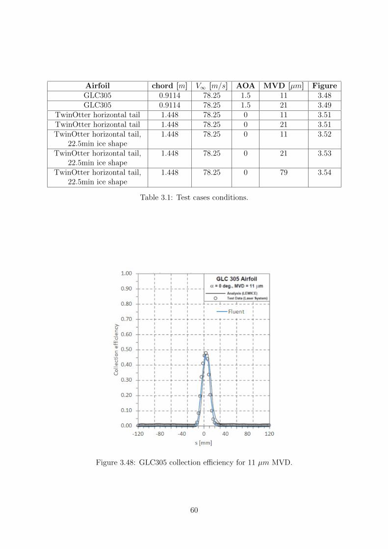
Airfoil chord [m] V∞ [m/s] AOA MVD [µm] FigureGLC305 0.9114 78.25 1.5 11 3.48GLC305 0.9114 78.25 1.5 21 3.49

TwinOtter horizontal tail 1.448 78.25 0 11 3.51TwinOtter horizontal tail 1.448 78.25 0 21 3.51TwinOtter horizontal tail,

22.5min ice shape1.448 78.25 0 11 3.52

TwinOtter horizontal tail,22.5min ice shape

1.448 78.25 0 21 3.53

TwinOtter horizontal tail,22.5min ice shape

1.448 78.25 0 79 3.54

Table 3.1: Test cases conditions.

Figure 3.48: GLC305 collection efficiency for 11 µm MVD.

60

Figure 3.49: GLC305 collection efficiency for 21 µm MVD.

Figure 3.50: Collection efficiency for 11 µm MVD on the Twin Otter horizontal tailsection.

61

Figure 3.51: Collection efficiency for 21 µm MVD on the Twin Otter horizontal tailsection.

Figure 3.52: Collection efficiency for 11 µm MVD on a simulated 22.5 minutes ice shapeon the Twin Otter horizontal tail section.

62

Figure 3.53: Collection efficiency for 21 µm MVD on a simulated 22.5 minutes ice shapeon the Twin Otter horizontal tail section.

Figure 3.54: Collection efficiency for 79 µm MVD on a simulated 22.5 minutes ice shapeon the Twin Otter horizontal tail section.

63

3.6 Thermodynamic balance

The solution of the thermodynamic balance on the surface is the core of the ice ac-cretion simulation. Indeed, the result of its solution is the freezing fraction at each airfoillocation, which translates in a local ice thickness. The solution of the balance is imple-mented in Fluent by means of a user defined function, because it was not possible tosimulate ice accretion in Fluent. The user defined function is launched when the flow fieldsolution has been obtained and the particle tracking module has been executed. For thefirst time step also the initial surface temperature has been computed, as indicated in sec-tion 2.4.1. Therefore, when the thermodynamic balance is solved, the flow variables, theheat transfer coefficient, obtained as indicated in 3.3, and the mass of impinging water,derived from the particle tracking described in 3.5, are known at each airfoil location.

The module is implemented with a udf that is executed outside the Fluent solutionprocess, so that the variables of interest do not vary in the execution. The solution ofequation (2.18) and (2.28) begins at the stagnation point, where it is assumed that thereis no runback water. At each body location, defined by a mesh face, the contribute ofthe energy and mass terms, detailed in 2.4, is computed, and are used to determine thelocal freezing fraction. Using the freezing fraction and the user input of time step lengththe mass of water freezing at a given location is determined; consequently, with the icedensity, also the local ice thickness. Also the mass flux of runback water leaving thecontrol volume can be computed from the solution of the mass balance, using the inputof freezing fraction and icing mass. Finally, the temperature on the initial surface, the icethickness and the energy and mass terms are used to calculate the temperature on theiced surface, which is obtained considering the effect of conduction through the ice layer.

This process is then repeated for the mesh face immediately downstream, where themass of runback water entering the volume is equal to the mass flux of runback waterleaving the preceding volume. At the end of the procedure the parameters characteriz-ing the ice accretion are therefore defined, and are subsequently used to determine thegeometry of the iced surface. Thus, for each face of the mesh has been defined:

• Freezing fraction.

• Mass of freezing water.

• Ice thickness.

• Temperature on the iced surface.

Finally, the user defined function prints in external files the energy and mass fluxesused to solve the thermodynamic balance as well as the parameters derived, like thefreezing fraction and the ice thickness.

64

3.7 Accretion algorithm

The solution of the energy and mass balance on the airfoil yields the ice thickness tobe added at each location. Because the thermodynamic balance is solved in a controlvolume, the output thickness can be associated with the thickness at the center of theface; the mesh instead is defined by the position of nodes, therefore it is first necessaryto compute the thickness to be added at each node. The node thickness is obtained byaveraging the ice thickness computed at the node adjacent faces, as in equation (3.13).

bnode =b(i) + b(i+1)

2(3.13)

Figure 3.55: Illustration of ice accretion procedure.

The local ice thickness have to be converted in a pair of coordinates, so that the nodesposition of the iced geometry can be computed. Therefore, the direction of accretion mustbe defined, and is obtained averaging the normals of the node adjacent face; this is givenby equation (3.14), where α is the angle defining the face normal.

α =α(i) + α(i+1)

2(3.14)

65

Using the thickness and direction of accretion, computed with equation (3.13) and(3.14), is then possible to compute the new coordinates of each node, that is:

xt+1 = xt + bnode cos(α) (3.15)

yt+1 = yt + bnode sin(α) (3.16)

When the iced geometry has been computed the accretion algorithm checks that thereis no intersection in the iced geometry; therefore, IceMAP 2D determines for each pair ofsegments, excluding the two adjacent segments, whether they intersect. If an intersectionis found all of the segments between the two intersecting are removed. Figure 3.56 illus-trates the procedure used: in red the calculated ice shape is intersecting in two differentposition, while in blue the final ice shape shows that the intersecting segments have beeneliminated.

x [m] #10-3

1 1.5 2 2.5 3

y [m

]

#10-3

-10.5

-10

-9.5

-9Ice accretion with intersectionIce accretion without intersection

Figure 3.56: Illustration of the procedure to remove intersections.

66

3.8 Mesh modification and control

The dynamic mesh feature available in Fluent allows to move the nodes positions ofa wall with respect to other cell zones and to adjust the mesh accordingly. The motionof the nodes is governed by a user defined function, using the coordinates computed in3.7. This has the advantage that the flow calculation is restarted from the solution of thepreceding time step; because the difference between the geometries are not excessivelylarge, the convergence of the solution is faster than it would be reinitializing the solution.Additionally, the time required to recreate the geometry and the mesh is eliminated,because the same mesh is reused for the successive time step. Thanks to the speed ofthe mesh modification process and solution computation this is the preferred method toadapt the mesh to the new geometry.

The morphed mesh, though, has to satisfy certain quality requirements to ensure thatFluent can compute a flow solution properly, therefore some of the properties of the meshare controlled. Specifically, volumes, skewness and face length on the airfoil are verifiedafter each mesh modification. These are the parameters with more effect on the solutionprocess, in that they can prevent Fluent from computing a proper flow solution. If theseparameters are not satisfied, like in figure 3.57, the domain is remeshed, figure 3.58, withthe procedure described in 3.2 which guarantees sufficient quality.

Figure 3.57: Example of mesh morphed in Fluent, with highly skewed cells and negativevolumes.

A mesh containing negative volumes will lead to divergence in the solution process,and for this reason they must be eliminated. Therefore, the quality check of the meshbegins with a control on the cells volume, and if any volumes is non positive the domain

67

Figure 3.58: Domain remeshed, satisfying the quality requirements.

is remeshed.Next the segments length is verified. Indeed, when ice grows on the surface the length

of a segment increases, but at some point will reach an excessive length; as a consequencesufficient definition of the surface may be lost and the flow field solution may not be ac-curate. Therefore, the ratio between the actual length and initial face length is computedto ensure that it does not exceed a given value. This is given in (3.17), where ∆Lmax isa user input.

dst+∆t

dst< ∆Lmax (3.17)

In this case the domain is remeshed, and the surface is divided in faces of length specifiedin input. In the script ∆Lmax was generally set at value between 1.5 and 2; when settingthe maximum allowed elongation of faces the same principles illustrated in section 3.2.1apply. Therefore, the maximum face length should generally not exceed a value of 2 mm,in order to ensure that the mesh is sufficiently fine at all the time steps.

Finally the mesh equiangular skewness, defined by equation (3.18), is checked.

skewness = max

[Θmax −Θe

180−Θe

,Θe −Θmin

Θe

](3.18)

Where Θe is the angle for an equiangle (ideal) cell, thus 60 degrees for triangular cells and90 degrees for quadrilateral cell. The skewness determines how close to ideal a cell is; avalue of 0 indicates an equilateral cell (best), while a value of 1 indicates a degenerate cell,which are characterized by nodes almost collinear. Highly skewed cell should be avoidedbecause they can compromise the accuracy of the solution; a maximum value of 0.85 is

68

generally accepted for quadrilateral cell, and triangular cells should not have skewnessabove 0.9. A single skewed cell does not generally alter significantly the solution, thus inIceMAP 2D a small percentage of cells is allowed skewness above a given threshold. Boththe threshold skewness and the percentage of skewed cells allowable is settable by the user.In the test cases, the threshold value was set at 0.75, while the maximum percentage was0.005%; these are also the default values in the script, and generally ensured an acceptablemesh quality.

69

Chapter 4

Results

The ice accretion simulation tool, IceMAP 2D, has been tested against both experi-mental data and test cases available in literature. The experimental ice shapes used forthe comparison have been obtained at the NASA Icing Research Tunnel and are presentedin [20], [19] and [17]. The analytical ice shape have been obtained from different icingsoftware and are also reported in literature; these are LEWICE[20][19][17], which is a wellvalidated icing software developed by NASA, TRAJICE2[19], developed by DRA, andONERA[19]. In some cases the simulated ice shape have been computed using LewIntand 1 no experimental ice shape is available as the test conditions were not found inliterature. Therefore, in the chapter with ice shapes and discussions is indicated whetherLEWICE, and thus data from literature, or LewInt is used.

Four different airfoils have been considered: a NACA 0012 symmetric airfoil, visiblein figure 4.1, a NACA 0015 symmetric airfoil, visible in figure 4.2, a non symmetric thinairfoil, figure 4.3 and an AgustaWestland proprietary airfoil. For the NACA 0012 airfoiltwo different chord length have been considered: this allowed to represent both smallertail rotor blade (using a chord of 0.152 m) and main rotor blade, considering a chord of0.53 m. The size of the body also influences the amount of icing accreting, mainly becauseof the different collection efficiency; for the NACA 0012 the differences resulting from thedifferent chord can therefore be analysed. A thick NACA 0015, with chord length of0.35 m, was selected, in order to also simulate thicker rotor blade. The GLC 305 airfoilconsidered has a chord length of 0.91 m and is representative of airfoil typically employedin wings. Finally a non symmetric AgustaWestland airfoil2 has been used, to verify thebehaviour of the tool with the type of airfoil used for helicopter; for this airfoil the originalgeometry has not been plotted.

To ensure repeatability of the shapes obtained the timestep used for each run wasselected using the procedure described in 4.1; in section 4.2 the test conditions, the iceshapes are presented and discussed.

1LewInt integrates the ice accretion code LEWICE (version 3.2.2) with icing analysis tools and auto-mated plotting. A fully functioning version of LewInt with LEWICE can be freely downloaded for a trialperiod.

2The shape and size of the airfoil are not reported because they are property of AgustaWestland andcan not be disclosed.

70

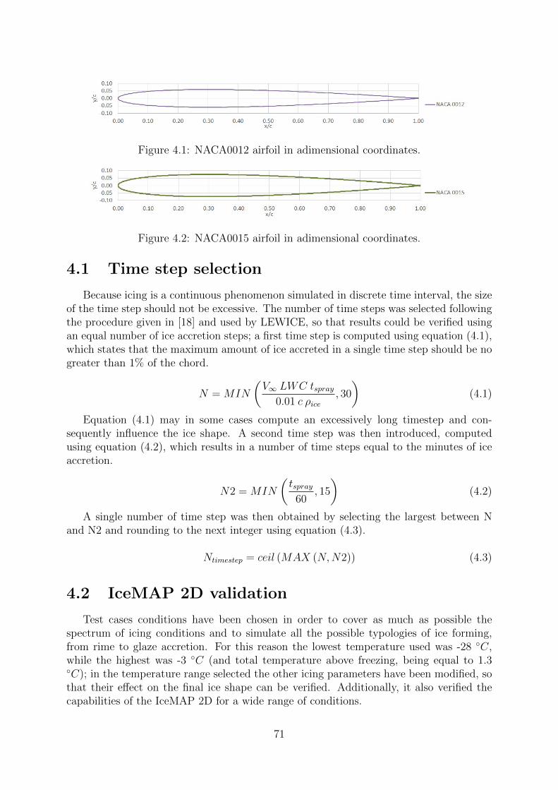
Figure 4.1: NACA0012 airfoil in adimensional coordinates.

Figure 4.2: NACA0015 airfoil in adimensional coordinates.

4.1 Time step selection

Because icing is a continuous phenomenon simulated in discrete time interval, the sizeof the time step should not be excessive. The number of time steps was selected followingthe procedure given in [18] and used by LEWICE, so that results could be verified usingan equal number of ice accretion steps; a first time step is computed using equation (4.1),which states that the maximum amount of ice accreted in a single time step should be nogreater than 1% of the chord.

N = MIN

(V∞ LWC tspray

0.01 c ρice, 30

)(4.1)

Equation (4.1) may in some cases compute an excessively long timestep and con-sequently influence the ice shape. A second time step was then introduced, computedusing equation (4.2), which results in a number of time steps equal to the minutes of iceaccretion.

N2 = MIN

(tspray

60, 15

)(4.2)

A single number of time step was then obtained by selecting the largest between Nand N2 and rounding to the next integer using equation (4.3).

Ntimestep = ceil (MAX (N,N2)) (4.3)

4.2 IceMAP 2D validation

Test cases conditions have been chosen in order to cover as much as possible thespectrum of icing conditions and to simulate all the possible typologies of ice forming,from rime to glaze accretion. For this reason the lowest temperature used was -28 ◦C,while the highest was -3 ◦C (and total temperature above freezing, being equal to 1.3◦C); in the temperature range selected the other icing parameters have been modified, sothat their effect on the final ice shape can be verified. Additionally, it also verified thecapabilities of the IceMAP 2D for a wide range of conditions.

71

Figure 4.3: GLC305 airfoil in adimensional coordinates.

The icing conditions tested were selected in order to be also representative of the flightconditions typical of helicopter operations, especially for the main rotor. Helicopter mainrotor blades are subject to large variation in angle of attack and Mach number: the bladetip on the advancing side generally operates at low angle of attack and Mach numberof 0.8, while on the retreating side it operated at angles of attack up to 10 degrees andMach number less than 0.4. These conditions can be averaged for a single revolution, toprovide a single representative icing conditions; considering that the blade tip is generallyless exposed to icing, as the kinetic heating due to the high speed limits the accretion ofice, and that the Mach number is higher at tip, the average angle of attack is about 5degrees and the Mach number is roughly 0.4.

In the temperature range selected the following parameters have been modified:

• Airspeed: from 67 m/s to 130 m/s, corresponding to Mach 0.4. No experimentalice shape were found in literature for higher Mach number, thus test cases at higherMach number were not simulated.

• Liquid water content: from 0.4 g/m3 to 1 g/m3. The value of 1 g/m3 is similar tothe maximum value expected in icing conditions and therefore leads to large amountof ice formation.

• Droplets diameter: from 15 µm to 38 µm. The 15 µm is the minimum size prescribedfor icing certification, and the the range selected is representative of the dimensionsmostly affecting airfoils.

• Angle of attack: from -2.5◦ to 8.5◦.

• Accretion time: from 2 to 45 minutes.

The test conditions also allowed to test the capabilities and robustness of the tool: indeed,extremely long accretion time, up to 45 minutes, and have been combined with highexternal temperature (-10 ◦C) and high angle of attack (6◦). These icing conditions leadsto wet accretion with large horns on the surface, which are the most critical conditionsto simulate. The tool worked properly also under this demanding conditions, and stillproduced an acceptable ice shape. Generally, though, ice is not allowed to grow forthat long, as de icing systems will cyclically remove the accretion thus leaving a cleansurface. Additionally, at lower temperature the accretion will have more and more rimecharacteristics, resulting in a streamlined accretion with no runback water on the surface.For these conditions the simulation is generally not as complex, and therefore it is expectedthat the code should be stable and reliable for all conditions.

72

The following ice shapes have been obtained for a symmetric NACA 0012 airfoil atincreasing temperature while the other parameters remain unchanged. The results ofIceMAP 2D has been compared with the output of LewInt and no data are available inliterature for the following conditions:

Run Rime Run Mixed Run GlazeAirfoil NACA 0012

chord [m] 0.53Figure 4.4 4.6 4.8

AOA [◦] 0V∞ [m/s] 67.056T∞ [K] 246.15 254.15 262.15

LWC [g/m3] 0.99MVD [µm] 38

t [min] 7

Figure 4.4, 4.6 and 4.8 show the effect of increasing temperature, while the othervariables remain unchanged; due to the high water loading ice shows glaze characteristicsalready at -18 ◦C, which are even more clear at -10 ◦C; yet the amount of runbackwater does not largely affects the icing limits, which remain almost unchanged in allconditions. Compared to LEWICE, the thickness at the leading edge is comparable forall the conditions, while some differences are visible at higher temperature in the hornsize and position. Specifically, in LEWICE the horns appear to form at a further locationwhile in IceMAP 2D they are closer to stagnation.

Because of the lack of an experimental ice shape to compare the simulated accretionno judgement can be expressed on the quality of the final result. In any case, the shapecomputed with IceMAP 2D and LEWICE are similar, and an experimental ice shapeobtained at the given conditions should be significantly different.

For these runs also the pressure coefficient for the iced shape is compared with theoutput from LEWICE. The pressure coefficient shows a similar trend for all cases, butsome differences in peaks are visible. These may be attributed to the differences in theshape computed, as the horns are positioned in the area where the largest discrepanciesare visible. Additionally, for the rime condition, the coefficient of pressure for the icedairfoil has been computed using either the mesh used in the accretion process and theaerodynamic mesh. In this condition the computed coefficient is extremely similar, butmay still result in some differences in the computation of the aerodynamic coefficients.

73

Figure 4.4: Run: rime. NACA0012, V∞ = 67.056 m/s, T∞ = 246.15 K, AOA = 0◦, LWC= 0.99 g/m3, MVD = 38 µm, t = 7 min.

Figure 4.5: Coefficient of pressure on iced airfoil for run rime computed with two differentmeshes and compared with LEWICE.

74

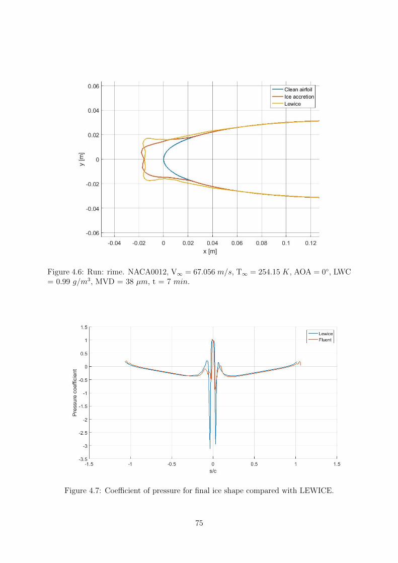
Figure 4.6: Run: rime. NACA0012, V∞ = 67.056 m/s, T∞ = 254.15 K, AOA = 0◦, LWC= 0.99 g/m3, MVD = 38 µm, t = 7 min.

Figure 4.7: Coefficient of pressure for final ice shape compared with LEWICE.

75

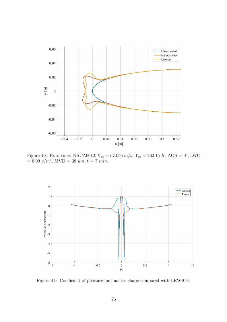
Figure 4.8: Run: rime. NACA0012, V∞ = 67.056 m/s, T∞ = 262.15 K, AOA = 0◦, LWC= 0.99 g/m3, MVD = 38 µm, t = 7 min.

Figure 4.9: Coefficient of pressure for final ice shape compared with LEWICE.

76

The following ice shapes have been obtained for a symmetric NACA 0012 airfoil atincreasing temperature while the other parameters remain unchanged. The results ofIceMAP 2D has been compared with the output of LEWICE and experimental dataavailable in literature for the following conditions:

Run 425 Run 11 Run 112 Run 118 Run 122 Run 421Airfoil NACA 0012

chord [m] 0.53Figure 4.10 4.11 4.12 4.13 4.14 4.15

AOA [◦] 4V∞ [m/s] 67.16 67.056 67.056 67.056 67.056 67.1T∞ [K] 244.51 253.69 259.84 263.14 265.35 268.4

LWC [g/m3] 1MVD [µm] 20

t [min] 6

The icing conditions for figure 4.10 to 4.15 are similar to those of 4.4, 4.6 and 4.8,but the airfoil is at 4 degrees and droplet size is almost halved. The total accretiontime has also been reduced to 6 minutes. In these cases (and all of the following) also anexperimental ice shape is available. In run 4.10 the accretion is of type rime, but comparedto 4.4 the positioning of the maximum thickness has slightly moved on the lower side ofthe airfoil due to the angle of attack. Therefore the ice shape is not symmetrical, and theicing limits on the suction and pressure side are different; additionally, the smaller particlesalso result in a larger impinged airfoil surface. Comparison with experimental data andLEWICE shows good agreement for both the icing limit and the maximum thickness anddirection. Compared with LEWICE IceMAP 2D shows only minor differences, as can beexpected in a rime accretion.

When free stream temperature reaches -20 ◦C, in figure 4.11, a limited amount ofrunback water starts to appear; temperature is similar to that in 4.6, as can be expectedconsidering that only the angle of attack and the particle size have changed. The icedsurface computed with IceMAP 2D shows more irregularities, but there is still goodagreement with experimental data for icing limit and maximum thickness.

Runback water increases when temperature reaches -13 ◦C, as in figure 4.12, but inthis case IceMAP 2D predicts the formation of a distinct horn on the lower side which isnot visible in the experimental shape. A similar effect, although less evident, is visible infigure 4.13. In both cases the thickness at stagnation and icing limits are comparable withthe experimental ice shape, as well as the ice formation on the upper side of the airfoil.The differences are probably caused by the modelling of the water film and the thermalexchange between water and air; indeed, the horn formation is caused by the freezingof runback water, and therefore a correct value of surface roughness and heat transfercoefficient can impact the type of ice growing. Also the modelling of the film flow maybe responsible for differences, which in the present work is computed without consideringthe effect of air shear. In these cases also LEWICE exhibit some clear differences withthe experimental ice shape, although the thickness location is different compared withIceMAP 2D. In LEWICE more ice is predicted on the upper horn, while the lower accretionis underpredicted.

77

In figure 4.14 the air temperature is further increased at -7 ◦C, and the ice shape com-puted in IceMAP 2D has significantly improved compared to previous runs; the horns onthe lower side is not visible, because convective and evaporative cooling are not sufficientto freeze the water film, which can flow further aft. This is also visible on the upperhorn, which has moved further away from the stagnation point. In this case IceMAP 2Dcompares favourably with the experimental ice shape, as icing limits, ice thickness anddistribution are similar to those tested. Compared to LEWICE, in this condition IceMAP2D also provides a better representation of the actual accretion, as the upper horn andlower accretion is more accurate.

In run 421, figure 4.15, the higher temperature (approximately -4 ◦C) has a dramaticeffect on the final ice formation, because the amount of heating on the airfoil impedes theformation of distinctive horns; in these conditions, the water film mostly affects the extentof the iced surface, which compared to previous runs has increased on both the upper andlower surface. A significant amount of ice is still forming on the airfoil, but the maximumthickness is less than in previous cases. Although the horn on the upper side and thethickness of ice near stagnation are marginally under estimated, the icing limit, especiallyon the lower side are correctly captured by IceMAP 2D; instead, LEWICE seems to underestimate not only the amount of ice accreting but also the icing limit on the lower surface.

x/c-0.05 0 0.05 0.1 0.15 0.2

y/c

-0.05

0

0.05

0.1CleanExperimentalLEWICEIceMAP 2D

Figure 4.10: Run: 425. NACA0012, V∞ = 67.1 m/s, T∞ = 244.51 K, AOA = 4◦, LWC= 1 g/m3, MVD = 20 µm, t = 6 min.

78

x/c-0.06 -0.04 -0.02 0 0.02 0.04 0.06 0.08 0.1 0.12 0.14

y/c

-0.06

-0.04

-0.02

0

0.02

0.04

0.06

0.08

0.1CleanExperimentalLEWICEIceMAP 2D

Figure 4.11: Run: 11. NACA0012, V∞ = 67.056 m/s, T∞ = 253.69 K, AOA = 4◦, LWC= 1 g/m3, MVD = 20 µm, t = 6 min.

x/c-0.06 -0.04 -0.02 0 0.02 0.04 0.06 0.08 0.1 0.12 0.14

y/c

-0.06

-0.04

-0.02

0

0.02

0.04

0.06

0.08

0.1CleanExperimentalLEWICEIceMAP 2D

Figure 4.12: Run: 112. NACA0012, V∞ = 67.056 m/s, T∞ = 259.8 K, AOA = 4◦, LWC= 1 g/m3, MVD = 20 µm, t = 6 min.

79

x/c-0.06 -0.04 -0.02 0 0.02 0.04 0.06 0.08 0.1 0.12

y/c

-0.06

-0.04

-0.02

0

0.02

0.04

0.06

0.08

0.1CleanExperimentalLEWICEIceMAP 2D

Figure 4.13: Run: 118. NACA0012, V∞ = 67.056 m/s, T∞ = 263.14 K, AOA = 4◦, LWC= 1 g/m3, MVD = 20 µm, t = 6 min.

x/c-0.06 -0.04 -0.02 0 0.02 0.04 0.06 0.08 0.1 0.12 0.14

y/c

-0.06

-0.04

-0.02

0

0.02

0.04

0.06

0.08CleanExperimentalLEWICEIceMAP 2D

Figure 4.14: Run: 122. NACA0012, V∞ = 67.056 m/s, T∞ = 265.35 K, AOA = 4◦, LWC= 1 g/m3, MVD = 20 µm, t = 6 min.

80

x/c-0.05 0 0.05 0.1 0.15 0.2 0.25

y/c

-0.05

0

0.05

0.1

CleanExperimentalLEWICEIceMAP 2D

Figure 4.15: Run: 421. NACA0012, V∞ = 67.1 m/s, T∞ = 268.4 K, AOA = 4◦, LWC =1 g/m3, MVD = 20 µm, t = 6 min.

81

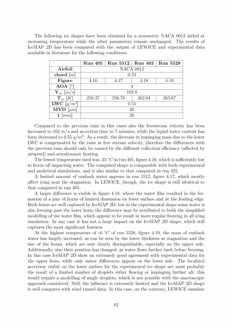
The following ice shapes have been obtained for a symmetric NACA 0012 airfoil atincreasing temperature while the other parameters remain unchanged. The results ofIceMAP 2D has been compared with the output of LEWICE and experimental dataavailable in literature for the following conditions:

Run 405 Run 5512 Run 403 Run 5528Airfoil NACA 0012

chord [m] 0.53Figure 4.16 4.17 4.18 4.19

AOA [◦] 4V∞ [m/s] 102.8T∞ [K] 250.37 256.78 262.04 265.67

LWC [g/m3] 0.55MVD [µm] 20

t [min] 20

Compared to the previous runs in this cases also the freestream velocity has beenincreased to 102 m/s and accretion time to 7 minutes, while the liquid water content hasbeen decreased to 0.55 g/m3. As a result, the decrease in impinging mass due to the lowerLWC is compensated by the raise in free stream velocity, therefore the differences withthe previous runs should only be caused by the different collection efficiency (affected byairspeed) and aerodynamic heating.

The lowest temperature used was -23 ◦C in run 405, figure 4.16, which is sufficiently lowto freeze all impacting water. The computed shape is comparable with both experimentaland analytical simulations, and is also similar to that computed in run 425.

A limited amount of runback water appears in run 5512, figure 4.17, which mostlyaffect icing near the stagnation. In LEWICE, though, the ice shape is still identical tothat computed in run 405.

A larger difference is visible in figure 4.18, where the water film resulted in the for-mation of a pair of horns of limited dimension on lower surface and at the leading edge.Both horns are well captured by IceMAP 2D, but in the experimental shape some water isalso freezing past the lower horn; the difference may be attributed to both the simplifiedmodelling of the water film, which appear to be result in more regular freezing in all icingsimulation. In any case it has not a large impact on the IceMAP 2D shape, which stillcaptures the most significant features.

At the highest temperature of -6 ◦C of run 5528, figure 4.19, the mass of runbackwater has largely increased, as can be seen by the lower thickness at stagnation and thesize of the horns, which are now clearly distinguishable, especially on the upper side.Additionally, also their position has changed, as water flows further back before freezing.In this case IceMAP 2D show an extremely good agreement with experimental data forthe upper horn, while only minor differences appear on the lower side. The localizedaccretion visible on the lower surface for the experimental ice shape are most probablythe result of a limited number of droplets either flowing or impinging further aft; thiswould require a modelling of single droplets, which is not possible with the macroscopicapproach considered. Still, the influence is extremely limited and the IceMAP 2D shapeis well compares with wind tunnel data. In this case, on the contrary, LEWICE simulate

82

a significant amount of water freezing on the upper horn, which largely alter the finalaccretion.

x/c-0.05 0 0.05 0.1 0.15

y/c

-0.06

-0.04

-0.02

0

0.02

0.04

0.06

0.08

0.1CleanExperimentalLEWICEIceMAP 2D

Figure 4.16: Run: 405. NACA0012, V∞ = 102.8 m/s, T∞ = 250.37 K, AOA = 4◦, LWC= 0.55 g/m3, MVD = 20 µm, t = 7 min.

83

x/c-0.05 0 0.05 0.1 0.15

y/c

-0.06

-0.04

-0.02

0

0.02

0.04

0.06

0.08

0.1

CleanExperimentalLEWICEIceMAP 2D

Figure 4.17: Run: 5512. NACA0012, V∞ = 102.8 m/s, T∞ = 256.78 K, AOA = 4◦, LWC= 0.55 g/m3, MVD = 20 µm, t = 7 min.

x/c0 0.05 0.1 0.15

y/c

-0.06

-0.04

-0.02

0

0.02

0.04

0.06

0.08

0.1 CleanExperimentalLEWICEIceMAP 2D

Figure 4.18: Run: 403. NACA0012, V∞ = 102.8 m/s, T∞ = 262.04 K, AOA = 4◦, LWC= 0.55 g/m3, MVD = 20 µm, t = 7 min.

84

x/c-0.04 -0.02 0 0.02 0.04 0.06 0.08 0.1 0.12 0.14 0.16

y/c

-0.06

-0.04

-0.02

0

0.02

0.04

0.06

0.08

0.1

CleanExperimentalLEWICEIceMAP 2D

Figure 4.19: Run: 5528. NACA0012, V∞ = 102.8 m/s, T∞ = 265.67 K, AOA = 4◦, LWC= 0.55 g/m3, MVD = 20 µm, t = 7 min.

85

The following ice shapes have been obtained for a symmetric NACA 0012 airfoil atincreasing accretion time while the other parameters remain unchanged. The resultsof IceMAP 2D has been compared with the output of LEWICE and experimental dataavailable in literature for the following conditions:

Run 411 Run 403Airfoil NACA 0012

chord [m] 0.53Figure 4.20 4.18

AOA [◦] 4V∞ [m/s] 102.8T∞ [K] 262.04

LWC [g/m3] 0.55MVD [µm] 20

t [min] 14 7

In run 411, figure 4.20, the conditions are the same as in run 403, figure 4.21, butthe accretion time has been increased to 14 minutes. Interestingly, in the 7 minutes iceaccretion the experimental lower icing limits are larger than in the 14 minutes run; this isprobably the result of the variability typically observable in icing tests under nominallyidentical conditions. Indeed, it is not possible to perfectly replicate the conditions (liketemperature and droplet diameter) in different runs; a further variability is due to theicing of individual droplets at slightly different position, which eventually leads to localizedaccretion at different location.

Because of the good agreement with the experimental shape for the lower accretiontime, also run 411 could be expected to provide as good a result. In this case, instead,IceMAP 2D under predicts the size of the horn near the leading edge of the airfoil, whilethe lower accretion is modelled correctly. The differences may be explained by the coarsemesh size (2 mm) used in the case; as a result, a single mesh element covers a large areaof the horn, reducing the definition of the geometry and leading to accretion in the wrongdirection. A finer size may in this run provide improvement of the result, but it has notbeen verified.

86

x/c-0.1 -0.05 0 0.05 0.1 0.15

y/c

-0.05

0

0.05

0.1

CleanExperimentalLEWICEIceMAP 2D

Figure 4.20: Run: 411. NACA0012, V∞ = 102.8 m/s, T∞ = 262.04 K, AOA = 4◦, LWC= 0.55 g/m3, MVD = 20 µm, t = 14 min.

x/c0 0.05 0.1 0.15

y/c

-0.06

-0.04

-0.02

0

0.02

0.04

0.06

0.08

0.1 CleanExperimentalLEWICEIceMAP 2D

Figure 4.21: Run: 403. NACA0012, V∞ = 102.8 m/s, T∞ = 262.04 K, AOA = 4◦, LWC= 0.55 g/m3, MVD = 20 µm, t = 7 min.

87

The following ice shapes have been obtained for a symmetric NACA 0012 airfoil atincreasing angle of attack while the other parameters remain unchanged. The results ofIceMAP 2D has been compared with the output of LEWICE and other icing tools andexperimental data available in literature for the following conditions:

Run DRA37 Run DRA38Airfoil NACA 0012

chord [m] 0.152Figure 4.22 4.23

AOA [◦] 0 8.5V∞ [m/s] 130.5T∞ [K] 260.7

LWC [g/m3] 0.5MVD [µm] 17.5

t [min] 2

In run DRA37, figure4.22, and DRA38, figure 4.23, a particularly small NACA 0012 isused, with chord length of 0.152 m, combined with a high velocity (130 m/s, Ma ≈ 0.4)and different angle of attack. Additionally, the ice shape is compared with experimentaldata, LEWICE and other icing software, developed respectively by DRA and ONERA.In 4.22 the angle of incidence was zero, but the computed ice shape was not perfectlysymmetrical; this the result of the non exact solution of the flow field, which also impactthe solution of thermodynamic balance and eventually affects the ice shape. However,IceMAP 2D simulated two large horns, typical of glaze accretion, in the correct direction;indeed, the horn thickness is comparable with experimental data, but not the thickness atstagnation point. Probably this is caused by the runback water modelling in IceMAP 2D;in the accretion module the water is expected to flow away from the stagnation point, butin reality this is an approximation that may be incorrect in some cases. At high velocityand glaze conditions, for example, this would result in water flowing from the stagnationpoint (located at the leading edge when the airfoil is at zero angle of attack) over thehorns; in reality, the film flow is governed by air shear which in this case would probablyprevent water from flowing past the horns, eventually freezing near the stagnation.

In run DRA38, figure 4.23, the angle of attack is 8.5 degrees, which is the highest angletested. In this case the computed accretion is similar to LEWICE, but the experimentaldata has feature that are not captured correctly. The feathers on the lower surface arethe result of localized ice accretion caused by the effects of single droplets, which in theicing tools are not modelled. A larger difference is visible near the leading edge, where thedirection of accretion is different. Beside the effect of surface roughness and the modellingof the water film, also the size of the mesh may have influenced the result. Although inthis case the size of the element used was 0.5 mm, because of the small airfoil size an evensmaller dimensions may be needed, but no test have been conducted.

88

Figure 4.22: Run: DRA37. NACA0012, V∞ = 130.5 m/s, T∞ = 260.7 K, AOA = 0◦,LWC = 0.5 g/m3, MVD = 17.5 µm, t = 2 min.

Figure 4.23: Run: DRA38. NACA0012, V∞ = 130.5 m/s, T∞ = 260.7 K, AOA = 8.5◦,LWC = 0.5 g/m3, MVD = 17.5 µm, t = 2 min.

89

The following ice shapes have been obtained for a symmetric NACA 0012 airfoil. Theresults of IceMAP 2D has been compared with the output of LEWICE and experimentaldata available in literature for the following conditions:

Run 412 Run 406Airfoil NACA 0012

chord [m] 0.53Figure 4.24 4.25

AOA [◦] 0V∞ [m/s] 102.8T∞ [K] 261.54 264.37

LWC [g/m3] 0.47 0.4MVD [µm] 30 20

t [min] 8.2 9.8

Run 412, figure 4.24, and run 406, figure 4.25, show the result of a longer icing expo-sure, reaching 8.2 and 9.8 minutes. In both cases the ice thickness is generally comparableas well as the icing limits. Larger differences exist for the longer accretion time, run 406,which also has the highest temperature; in this case the horn thickness on the uppersurface and the lower accretion are partly under estimated. However, the final ice shapeshows good agreement with experimental ice shape, and although LEWICE better modelthe horn it misses part of the accretion on the lower side of the airfoil.

x/c-0.05 0 0.05 0.1 0.15 0.2

y/c

-0.05

0

0.05

0.1

CleanExperimentalLEWICEIceMAP 2D

Figure 4.24: Run: 412. NACA0012, V∞ = 102.8 m/s, T∞ = 261.54 K, AOA = 4◦, LWC= 0.47 g/m3, MVD = 30 µm, t = 8.2 min.

90

x/c-0.05 0 0.05 0.1 0.15

y/c

-0.06

-0.04

-0.02

0

0.02

0.04

0.06

0.08

0.1

0.12CleanExperimentalLEWICEIceMAP 2D

Figure 4.25: Run: 406. NACA0012, V∞ = 102.8 m/s, T∞ = 264.37 K, AOA = 4◦, LWC= 0.4 g/m3, MVD = 20 µm, t = 9.8 min.

91

The following ice shapes have been obtained for a symmetric NACA 0015 airfoil. Theresults of IceMAP 2D has been compared with the output of LEWICE and experimentaldata available in literature for the following conditions:

Run 624963 Run 624966Airfoil NACA 0015

chord [m] 0.353Figure 4.26 4.27

AOA [◦] 0V∞ [m/s] 95.215 85.39T∞ [K] 262.85 263.07

LWC [g/m3] 0.75 0.77MVD [µm] 19 23.4

t [min] 10 10.8

In run 624963 and 624966, figure respectively 4.26 and 4.27, the airfoil used is athick NACA0015 of 0.35 m chord. Again, the conditions are typical of wet accretion,as can be seen by the large horn accreting at the leading edge. Although the two casesare different, the icing conditions are not significantly different and result in similar iceformation. The experimental ice shape shows two main large horns forming and additionalaccretions further aft. In both of these runs IceMAP 2D provide a more accurate resultthan LEWICE; the direction and thickness of the main horns is significantly closer to theexperimental, while the thickness at the leading edge is similar for both icing tools. Thesmaller ice formations past the two horns is not clearly visible in either analytical tools,although in IceMAP 2D a small ridge appears on both the upper and lower horns.

92

x/c-0.05 0 0.05 0.1 0.15 0.2

y/c

-0.1

-0.05

0

0.05

0.1

CleanExperimentalLEWICEIceMAP 2D

Figure 4.26: Run: 624963. NACA0015, V∞ = 95.215 m/s, T∞ = 262.85 K, AOA = 0◦,LWC = 0.75 g/m3, MVD = 19 µm, t = 10 min.

x/c-0.1 -0.05 0 0.05 0.1 0.15 0.2

y/c

-0.1

-0.05

0

0.05

0.1

CleanExperimentalLEWICEIceMAP 2D

Figure 4.27: Run: 624966. NACA0015, V∞ = 85.39 m/s, T∞ = 263.07 K, AOA = 0◦,LWC = 0.77 g/m3, MVD = 23.4 µm, t = 10.8 min.

93

The following ice shapes have been obtained for a GLC 305 airfoil. The results ofIceMAP 2D has been compared with the output of LEWICE and experimental dataavailable in literature for the following conditions:

Run 72701 Run 72703Airfoil GLC 305

chord [m] 0.91Figure 4.28 4.29

AOA [◦] 6V∞ [m/s] 90T∞ [K] 263.2

LWC [g/m3] 0.43 0.6MVD [µm] 20 15

t [min] 45 22.5

In run 72701, figure 4.28, the airfoil is 0.91 m chord GLC305, which is a particularlythin airfoil. Ice conditions are extremely demanding, as they include long accretion time,45 minutes, high angle of attack, 6 degrees, and high temperature, -10 ◦C. This is thelongest accretion time used with IceMAP 2D, and was divided in 15 time steps of threeminutes each. As an indication of the computation time required, the simulation took1 hour and 45 minutes with a serial computation, which is acceptable considering thatFluent is tasked with computing a flow field solution at each accretion. Indeed, most ofthe simulation time is due to flow field solution, while the ice accretion module, thereforeconsidering particle tracking, thermodynamic solution and update of the geometry andmesh takes roughly 1 minutes per time step.

IceMAP 2D successfully completed the simulation and provided an accurate ice shape,even if some differences can be seen. Specifically, these are in the area near the top horn,which is only partially visible in IceMAP 2D, and in the lower icing, where a smallaccretion is present. Still, the differences are not particularly large, especially consideringthe long accretion time. In the simulation process no errors were encountered, thusreducing the time step, at the cost of the simulation time, may also be a possibility toimprove the result obtained. Further, the fact that the ice shape is still comparable provesthat the approximations introduced in the modelling, like the simplification of the waterfilm flow, are reasonable and do not have a particularly large effect on the final ice shape.

Run 72703, figure 4.29, also is long accretion simulation of 22.5 minutes, at higherliquid water content (0.6 g/m3) and smaller droplet size (15 µm). Compared to run72701 the ice thickness at the leading edge is smaller, because of the lower icing time,but not halved as the accretion time because of the higher water content. In this casetherefore glaze feature, like horns, are more visible, because the increase of impingingwater is not coupled with an increase in icing in the impacting area. Water may flow andresult in larger area of the airfoil being affected by icing. In this case the horn thicknessis not significantly less than the experimental value, and its direction is almost correct;compared to LEWICE this provide a better approximation of the upper horn, while on thelower surface IceMAP 2D predicts the formation of a second horn which is as clear in theexperiments. Overall, also in this case the computed ice shape is comparable, includingfor what concern the icing limits.

94

x/c-0.05 0 0.05 0.1 0.15

y/c

-0.08

-0.06

-0.04

-0.02

0

0.02

0.04

0.06

0.08 CleanExperimentalLEWICEIceMAP 2D

Figure 4.28: Run: 072701. GLC305, V∞ = 90 m/s, T∞ = 263.2 K, AOA = 6◦, LWC =0.43 g/m3, MVD = 20 µm, t = 45 min.

x/c-0.08 -0.06 -0.04 -0.02 0 0.02 0.04 0.06 0.08 0.1 0.12

y/c

-0.08

-0.06

-0.04

-0.02

0

0.02

0.04

0.06

0.08CleanExperimentalLEWICEIceMAP 2D

Figure 4.29: Run: 072703. GLC305, V∞ = 90 m/s, T∞ = 263.2 K, AOA = 6◦, LWC =0.6 g/m3, MVD = 15 µm, t = 22.5 min.

95

The following ice shapes have been obtained for an AgustaWestland airfoil3. Theresults of IceMAP 2D has been compared with wind tunnel data for the following condi-tions:

Run AW5Airfoil AW

chord [m] -Figure 4.30

AOA [◦] -2.5V∞ [m/s] 92.6T∞ [K] 270.15

LWC [g/m3] 0.63MVD [µm] 25

t [min] 15

In run AW5, figure 4.30, ice accretion on a production helicopter airfoil developed byAgustaWestland is simulated. The temperature is the highest among those tested, beingequal to -3 ◦C, and total temperature is above freezing. As can be seen, the fact that thetotal temperature is above freezing is not sufficient to guarantee that no ice will grow.In this conditions water evaporation will cool the surface, eventually falling to zero andhence ice may accrete. A similar effect is simulated by IceMAP 2D, as ice grow overlarge areas of the airfoil, although the thickness is generally limited. A larger accretionis visible on the lower surface, which is simulated correctly by IceMAP 2D although in aslightly different position. Additional localized accretion are visible in the experimentalice shape on the upper surface, while the in the analytical shape the ice covers a largerarea of the airfoil and only has a limited thickness. The difference may be explained bythe simplification of the freezing model. Observations revealed that the flow of water oversurface is largely impacted individual surface roughness element, such as those caused byfreezing of small amount of water. In the model considered instead the surface roughnessdoes not directly impact the film flow, but influences the heat transfer coefficient andconsequently the rate of water freezing. As a result the ice forming is distributed overa wide surface area rather than concentrated in a small area where water initially froze.This effect though can not be easily modelled, as it would require a more microscopicmodelling of the icing surface to take into account the individual roughness elements.

3The shape and chord of the airfoil are not reported because they are property of AgustaWestlandand can not be disclosed.

96

Figure 4.30: Run: AW5. AW airfoil, V∞ = 92.6 m/s, T∞ = 270.15 K, AOA = -2.5◦,LWC = 0.63 g/m3, MVD = 25 µm, t = 15 min.

97

Chapter 5

Computation of aerodynamiccoefficients

IceMAP 2D also output the aerodynamic coefficients acting on the surface, which isa key performance indicator. As has been discussed, ice accretion leads to mass increaseand performance degradation, which are usually measured using the coefficient of lift anddrag. These are computed by default in IceMAP 2D for the final ice shape, but theuser may also utilize Fluent to compute the coefficient at a different time step; this isdone because of the different mesh is used to compute the aerodynamic coefficients andthe ice accretion. The result obtained analytically in Fluent have been validated withexperimental data[10] for iced airfoil from the Icing Research Tunnel. In the test casesconducted an iced NACA0012 airfoil with 0.53 m chord was used.

5.1 Rime conditions

The ice shape is first obtained for rime condition and at a fixed angle of attack.The coefficient of drag is then measured at different angles of attack and compared withexperimental data, obtained following a similar procedure. The external conditions forrime ice growth are as follows:

• Velocity 58.06 m/s.

• Static temperature 248.8 K.

• Angle of attack 4◦.

• Liquid water content 1 g/m3.

• Droplet diameter 12 µm.

• Spray time 5 min.

The final ice shape, computed in IceMAP 2D and experimental, is visible in 5.1. In thiscase IceMAP 2D was used with a coarser time step compared to the value that would beobtained using the procedure indicated in section 4.1, thus the ice shape may be differentusing a smaller time step. Still, the differences with the experimental ice shape are notlarge, being limited to the area on top of the ice growth.

98

AOA ◦ cd IRT cd Fluent-3 0.01268 0.012110 0.01172 0.010064 0.01077 0.010758 0.01610 0.0154011 0.03148 0.02201

Table 5.1: Coefficient of drag at different angles for rime ice shape.

When the ice shape has been obtained, the coefficient of drag of the airfoil is measuredat different angle of attack, so that an indication of the variability of drag coefficients andthe effects on the flow over the airfoil can be derived. Table 5.1 include the coefficient ofdrag measured at IRT and computed in Fluent

Figure 5.1: Final ice shape obtained for rime ice, Fluent and IRT.

The coefficient of drag for the iced and clean airfoil are also plotted in figure 5.2. Theincrease in drag is large for all conditions; for example, at zero angle of attack the dragraised to twice its corresponding clean value. Additionally, the increase can be extremelyfast, as the ice formed in five minutes.

The coefficient of drag computed in Fluent is comparable with experimental data forsmall angle of attack, but it is smaller at higher angle. In the wind tunnel, for high angleof attack, flow separation was observed, which lead to a substantial increase in drag; onthe contrary, in Fluent the flow remained attached at all conditions. This may be causedby the difference in the ice shape visible on the upper surface; indeed, the transitionbetween the iced surface and the airfoil appears to be smoother than in the experimentalconditions. This may have a large impact, especially at high angle of attack, because theflow separation is caused by the irregularities in the ice formation.

5.2 Glaze conditions

A second test has been conducted at higher temperature, resulting in a different typeof ice forming. For glaze ice accretion the ambient conditions are:

• Velocity 58.06 m/s.

99

Figure 5.2: Plot of coefficient of drag vs AoA for rime ice, Fluent and IRT.

• Static temperature 266.8 K.

• Angle of attack 4◦.

• Liquid water content 2.1 g/m3.

• Droplet diameter 20 µm.

• Spray time 5 min.

Figure 5.3: Ice shape obtained for glaze condition, IceMAP 2D and IRT.

Figure 5.3 shows the ice shape after the 5 minutes icing computed by IceMAP 2Dand used to compute the aerodynamic coefficient along with experimental accretion. Inthis case the shape is different from the previous case, because runback water has created

100

AOA ◦ cd IRT cd Fluent-3 0.02683 0.013250 0.02199 0.013744 0.02767 0.02244

5.5 0.03580 0.030068 0.07647 0.06605

Table 5.2: Coefficient of drag at different angles for glaze ice shape.

additional localized ice thickness on the lower side of the airfoil. Additionally, the distri-bution of ice has created a less streamlined surface. Therefore, the increase in coefficientof drag is also subject to a large increase compared to a clean NACA 0012. This is shownin table 5.2, which contains the coefficient of drag measured at IRT and computed inFluent, and in figure 5.4.

Figure 5.4: Plot of coefficient of drag vs AoA for glaze ice, Fluent and IRT.

Fluent under predicts the coefficient of drag at all angles; this can be explained bythe difference in the ice shape, visible in figure 5.3, and by the smoother surface obtainedin Fluent. This may be mitigated using a smaller mesh size, especially near the leadingedge, so that even smaller feature typical of glaze ice can be modelled. Still, the resultscomputed in Fluent are similar to the experimental value, and have general validity.

In this condition the coefficient of drag is more than doubled at zero angle of attack,and the difference becomes even larger at increasing angle of attack. Indeed, in the IRTtests the flow over the entire upper surface separated at an angle of attack as low as 6degrees, while for the clean airfoil stall begins above 10 degrees. A similar condition isalso apparent in Fluent, as the coefficient of drag has a similar trend. In figure 5.6 thevelocity flow field over the upper surface of the airfoil, computed in Fluent, is visualizedusing vectors; the airfoil is set at 5.5 degrees, and the flow separation is already affecting alarge portion of the airfoil. This has also effect on the numerical value of the coefficient of

101

Figure 5.5: Coefficient of lift for a clean and iced NACA 0012 airfoil.

drag: at 5.5 degrees, for example, Fluent computes a value that is more than three timeslarger than the corresponding clean value and can be explained by the flow separationover the suction side.

Additionally, in Fluent also the coefficient of lift has been computed for the iced airfoilat different angle of attack. Also the lift characteristics of the airfoil are compromised bythe ice accretion, as can be seen in figure 5.5, even at low angle of attack. This furtherhighlight the issues outlined in the introduction, 1, and caused by the rapid accretion ofice on lifting surfaces. In this glaze condition, the drag more than doubled at all angle ofattack, while at the same time the lifting characteristics worsened. For icing on helicopterblade this problem would be further exacerbated by the variations in the angle of attackto which the blade is subject; indeed, for the advancing blade the angle of attack mayreach 10 degrees, which will result in the premature stall of the airfoil.

102

Figure 5.6: Vectors of velocity on the upper surface of the iced airfoil. Recirculation offlow over a large area at 5.5 degrees on a glaze ice accretion.

103

Chapter 6

Conclusions

A tool, IceMAP 2D, to simulate ice accretion has been successfully developed andintegrated in ANSYS Workbench; also the ice accretion module has been completelydeveloped and is embedded in Fluent. A minimal number of inputs are required toperform the simulation while the rest of the process is automatically executed. The finaloutput includes the iced geometry and the aerodynamic coefficients for the iced airfoil.

IceMAP 2D has proved to be capable of simulating ice accretion for a wide variety oficing conditions of interest. The tool has not been subject to failures and computationtime have been limited to less than 10 minutes per time step on a laptop. Therefore,a sensible number of icing conditions have been tested to verify the accuracy of thesimulation, including particularly demanding conditions, like long accretion time, highangle of attack and high temperature. The ice shapes obtained are overall comparable,not only for rime conditions but also in glaze conditions. Specifically, maximum thickness,presence of horns and their direction are computed correctly in the cases tested. Theusage of a CFD software to simulate the flow field and the icing model employed has thusresulted in a good agreement with experimental ice shapes.

A somewhat larger variability has been observed in the computation of the aerody-namic coefficients, which is generally limited at high angles of attack. Because in thisconditions flow separation is a significant part of the drag increase, small differences inthe computed ice shape can lead to large variations in the aerodynamic coefficients. Thenumber of test cases for which the coefficient of drag is available is limited, and thereforealso the coefficient of drag have been compared only in some cases. Additional tests, alongwith a refinement of the mesh could help better understand if the differences observed arecaused by difference in ice shape.

104

Chapter 7

Future development

Although IceMAP 2D has been successfully used to simulate ice accretion, a number ofimprovements could be done, to either improve the results or include additional features.

As has been observed in the mesh chapter, 3.2.1, the mesh size has an influence onthe computed ice accretion; indeed, using a mesh too coarse will result in the eliminationof ice feature, while using a mesh too fine will result in numerical difficulties. Therefore,a complete study of the variability of ice shape with respect to mesh size should beconducted, in order to provide better guidance in the choice of the mesh size.

An additional factor that affects the ice growth is the surface roughness and conse-quently the heat transfer coefficient; in the model considered a single value of surfaceroughness was employed, but it does not represents the actual local roughness. In Fluentit is possible to define a variable surface roughness for the surface of interest, and thisfeature may be used to impose a local value of roughness computed using the icing condi-tion at a given surface location. The use of a different turbulence model to compute theheat transfer coefficient and to obtain the flow solution leads in an increase in the overallcomputational time; using a kω − SST turbulence model for all the simulation will cutthe computation time, but testing is required to ensure that the heat transfer coefficient isstill accurate. The variability observed in 3.3 may be eliminated by a proper modificationof the turbulence model parameters available in Fluent. This, though, should not resultin the worsening of the boundary layer solution.

In glaze condition the water film has a significant impact on the ice shape, as it resultin large localized accretion (horns). The flow of the film is mainly governed by air shear,which in the current model is not considered. The inclusion may improve the ice shapewhen the presence of horns is particularly large, as in this case the simple flow model usedmay not provide an accurate modelling.

The inclusion of a more complex fluid flow model is also required in a three dimensionalextension of IceMAP 2D; in this conditions additional forces, like centrifugal forces forrotor blades, acting on the water film must be considered because they significantly impactthe flow direction and consequently the freezing location of runback water. If these forcesare neglected the capability of simulating ice accretion on more complex geometries wouldbe severely impeded. Fluent, in this respect, offer great flexibility, as also rotating objectcan be properly simulated, thus the ice accretion module would not require substantialwork. Additionally, the forces acting on the water film can be computed directly by Fluentin the solution process, thus ensuring that the modelling of forces, mass and energy fluxes

105

is as accurate as possible.An additional feature that may be implemented is the simulation of anti icing systems.

This should provide the capability to ensure that the anti icing system installed or designedis capable of maintaining the surface clean from ice. The system provides a heat flux tothe surface, which must be accounted for in the thermodynamic balance. The solutionyields the freezing and the surface temperature, which are the required parameters toensure that the surface remains clean from ice.

Finally, the model may be extended to larger size (SLD) by considering the effects ofparticle deformation, breakup and splashing which are significant in this range of size;this would result in a more realistic collection efficiency and impinging mass on the airfoil.Therefore, the smaller droplets resulting from breakup or splashing are simulated, thusconsidering that they may flow past the surface or impact on the surface at a differentlocation.

106

Appendix A

IceMAP 2D structure

A.1 List of input

It is first required to define the name of the folder where the file generated in thesolution process, by ANSYS Workbench and IceMAP 2D, are saved. The inputs requiredby IceMAP 2D for the icing simulation can be broadly divided in external condition (icingand freestream), geometry characteristic, mesh characteristic and mesh quality controls.

Ambient conditions required are:

• Freestream velocity.

• Freestream static temperature.

• Freestream static pressure.

• Angle of attack.

• Liquid water content.

• Mean volumetric diameter.

• Number of time steps.

• Accretion time per time step.

• x-position of water injection in the domain for the particle tracking module m. Y-coordinates are estimated using geometric information of the airfoil size and angleof attack.

Geometric informations required are:

• Chord length.

• Thickness to chord ratio. This is to be set only if the airfoil is NACA 4 digitsymmetric airfoil, as in this case the airfoil coordinate file is automatically generated.For other airfoil this parameter is not required, as the the geometry is defined byan external file.

107

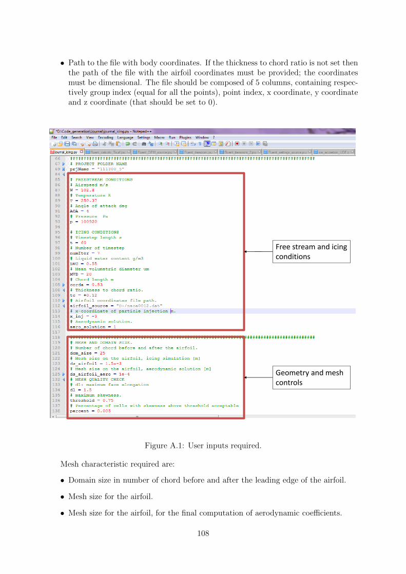
• Path to the file with body coordinates. If the thickness to chord ratio is not set thenthe path of the file with the airfoil coordinates must be provided; the coordinatesmust be dimensional. The file should be composed of 5 columns, containing respec-tively group index (equal for all the points), point index, x coordinate, y coordinateand z coordinate (that should be set to 0).

Free stream and icing conditions

Geometry and mesh controls

Figure A.1: User inputs required.

Mesh characteristic required are:

• Domain size in number of chord before and after the leading edge of the airfoil.

• Mesh size for the airfoil.

• Mesh size for the airfoil, for the final computation of aerodynamic coefficients.

108

Finally the controls used to check the mesh quality after each time step must bespecified:

• Maximum acceptable elongation of segments on the airfoil.

• Threshold skewness.

• Maximum percentage of cell with skewness above the threshold value acceptable.

These parameters are set directly in the script, as shown in figure A.1.

A.2 Solution steps

IceMAP 2D is written in Python and is executed as a script file in ANSYS Workbench.IceMAP 2D is responsible for the modification of the script and journal files necessaryaccording to the input supplied, the creation of the blocks in project schematic, launchingthe various application in a specified order and issuing commands through the scripts andjournal, and checking the mesh quality.

Figure A.2: Launching of the script in ANSYS Workbench. Also visible below the blocksthat will be created.

109

In the script and journal additional controls on the solution process may be accessedif the predefined values do not provide satisfactory results. The scripts required for thecreation of the mesh on the computational domain are:

• ”script geometry.js”: generates the computational domain in ANSYS DesignMod-eler, using the supplied airfoil geometry and domain size.

• ”script mesh.js”: generates, in ANSYS Meshing, the boundary discretization on theairfoil and on the far field used for the ice accretion simulation. The size of the meshis defined in the input parameters.

• ”script mesh aero.js”: generates, in ANSYS Meshing, the boundary discretizationon the airfoil and on the far field used for the computation of the aerodynamiccharacteristics. The size of the mesh is defined in the input parameters.

• ”tgrid journal.jou”: generates the volumetric mesh of the domain in Tgrid, usingthe boundary discretization supplied by ANSYS Meshing.

Tgrid is integrated in ANSYS Workbench using a configuration file, ”tgrid.xml”, whichdefines the properties of the block appearing in the project schematic. When the block isupdated a script, ”tgrid.py”, is executed and launches Tgrid; finally in Tgrid the journal”tgrid journal.jou” is executed.

The generated mesh is then imported in Fluent, where a number of journals are usedin the process. These are:

• ”Fluent settings.jou”: contains the settings required for the fluid flow simulation,including the free stream conditions supplied and the surface roughness, which isautomatically computed in IceMAP 2D.

• ”Fluent compute Tsurf.jou”: the journal is used to compute the surface temperatureon the airfoil before the first time step. It output a file with the temperaturedistribution over the airfoil, which is then read in Fluent and used for the actualicing simulation.

• ”Fluent iterations.jou”: contains the instruction required to compute the heat trans-fer coefficient at every time step. Therefore the appropriate turbulence model andsurface temperature is set before saving the heat transfer coefficient values at eachsurface location.

• ”Fluent iterations2.jou”: solves the fluid flow with the kω−SST turbulence modelto compute the forces acting on liquid droplets and the flow variables on the surface.

• ”Fluent DPM.jou”: contains the instructions required to launch the particle track-ing, the ice accretion module and the update of the geometry.

• ”Fluent aero coefficients.jou”: solution of the fluid flow for the computation of theaerodynamic coefficients.

The user defined functions required in the ice accretion process are written in a C file,”ice accretion UDF.c”, which is also supplied to Fluent and is responsible of:

110

• Initializing variables required in the simulation.

• Initializing particle position as defined in the inputs.

• Store particle data at impact, that is temperature and velocity of particles at impactand mass flow rate.

• Compute collection efficiency.

• Compute the energy and mass terms necessaries and solve the thermodynamic bal-ance, in order to compute at each surface location the freezing fraction, icing mass,ice thickness and temperature on the iced surface.

• Compute the position of the iced surface.

• Write in external file the variables of interest.

The previous files are saved in the folder for the project, so that they may be usedin case the user decides to continue a simulation manually. In this case the user is onlyrequired to launch in the proper order the scripts already present. Beside launching theprevious files IceMAP 2D also control the quality of the mesh at each time step to decidewhether the domain should be remeshed, and renames the output file of the user definedfunctions for later use.

A.3 List of output

At the end of each time step seven files are written, containing information from thethermodynamic balance and the iced geometry. These are:

• ”b data.txt”

• ”m data.txt”

• ”q data.txt”

• ”t data.txt”

• ”D mesh.txt”

• ”face pos.txt”

• ”flow data.dat”

IceMAP 2D also add an index representing the time step for which the file were written,thus for example ”m data2.txt” contains informations calculated at the second time step.In the files the information for each segment of the airfoil are listed. The face can beidentified by a unique index, written in all of the file, beginning at stagnation point andincreasing clockwise. Coupled with the face length, which is also output, can be used todefine a curvilinear coordinates system on the airfoil

”b data.txt” contains generic information on the ice accretion:

111

• Face index.

• Collection efficiency.

• Freezing fraction.

• Ice thickness.

• Number of particle impacts.

• Face length.

”m data.txt” stores the mass fluxes terms computed for the mass balance:

• Face index.

• Mass flux of impinging water.

• Runback water entering the face.

• Mass flux of evaporating water.

• Mass flux of sublimating water.

• Mass flux of water freezing.

• Freezing fraction.

• Face length.

”q data.txt” stores the energy fluxes terms computed for the energy balance:

• Face index.

• Energy flux due to convection.

• Energy flux due to aerodynamic heating.

• Energy flux due to evaporation.

• Energy flux due to sublimation.

• Energy flux due to the impact of particles.

• Energy flux due to internal energy of impinging water.

• Energy flux due to ruback water entering the face.

• Heat transfer coefficient.

• Freezing fraction.

• Face length.

”t data.txt” stores informations on the surface temperature:

112

• Face index.

• Surface temperature before ice accretion.

• Air temperature on the surface.

• Temperature on the ice accretion.

• Face length.

”D mesh.txt” stores informations on the nodes positions, used in the mesh modifica-tion in Fluent:

• Face index.

• x-coordinate of node after ice accretion.

• y-coordinate of node after ice accretion.

”face pos.txt” stores informations on position of the face centroid, used to output acoordinate file of the geometry:

• Face index.

• x-coordinate of face centroid before ice accretion.

• y-coordinate of face centroid before ice accretion.

• x-coordinate of face after ice accretion.

• y-coordinate of face after ice accretion.

• Face length.

”flow data.dat” stores informations on the calculated conditions at the edge of theboundary layer:

• Face index.

• Temperature at the edge of the boundary layer.

• Pressure at the edge of the boundary layer.

• Mach at the edge of the boundary layer.

• Velocity at the edge of the boundary layer.

• Face length.

When the aerodynamic coefficients on the iced airfoil have been computed an addi-tional file is written, ”Forces.dat”, which contains the axial and normal forces computedin Fluent for the airfoil as well as the axial and normal coefficients. These are computedconsidering a chord length of 1 m, thus must be divided by the chord length before beingused. Additionally, the computed forces and coefficients are divided in the contribute dueto pressure and viscosity.

113

A.4 Postprocessing

A MATLAB script can also be used to visualize the information provided in the outputfiles. The script require the path of the folder where the output files are located and thenumber of time steps that should be imported. Each column of the file is then plotted ina MATLAB figure. The abscissa of the figures is the adimensional surface length, startingfrom stagnation; surface length is considered positive on the upper airfoil surface, while isconsidered negative on the lower surface. The ice shape at different time steps is insteadplotted in dimensional coordinates, as in figure A.3

x [m]-0.02 0 0.02 0.04 0.06

y [m

]

-0.04

-0.03

-0.02

-0.01

0

0.01

0.02

Ice accretionClean airfoilTimestep 1Timestep 2Timestep 3Timestep 4Timestep 5Timestep 6Timestep 7

Figure A.3: Ice shape at different time steps for run 5528. Total accretion time 7 minutes,time step of 1 minutes.

The variables are labelled in order to indicate the time step at which they were com-puted. The mass (figure A.4) and energy (figure A.5) fluxes are adimensionalized withrespect to the local surface area, so that the local size of the element does not influencethe result; therefore the fluxes computed with different meshes may be compared directlywithout further computation.

114

s/c-0.2 -0.15 -0.1 -0.05 0 0.05 0.1 0.15 0.2

kg/m

2-s

0

0.005

0.01

0.015

0.02

0.025

0.03

0.035

0.04m impinging

Timestep 1Timestep 2Timestep 3Timestep 4Timestep 5Timestep 6Timestep 7

Figure A.4: Impinging mass flux at different time steps for run 5528. Total accretion time7 minutes, time step of 1 minutes.

115

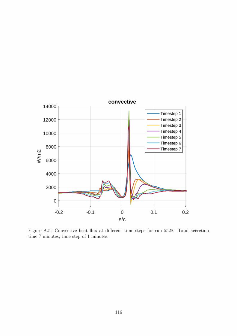
s/c-0.2 -0.1 0 0.1 0.2

W/m

2

0

2000

4000

6000

8000

10000

12000

14000convective

Timestep 1Timestep 2Timestep 3Timestep 4Timestep 5Timestep 6Timestep 7

Figure A.5: Convective heat flux at different time steps for run 5528. Total accretiontime 7 minutes, time step of 1 minutes.

116

Bibliography

[1] JT Cansdale and RW Gent. Ice accretion on aerofoils in two-dimensional compressibleflow-a theoretical model. Royal Aircraft Establishment Technical Report, 82128, 1983.

[2] HW Coleman, BK Hodge, and RP Taylor. A re-evaluation of schlichting’s surfaceroughness experiment. Journal of Fluids Engineering, 106(1):60–65, 1984.

[3] Ansys Fluent. 16.0 udf manual. Ansys Inc, 2015.

[4] RW Gent. Trajice 2, a combined water droplet and ice accretion prediction programfor aerofoil, royal aerospace establishment(rae) technical rept. tr 90054, farnborough,hampshire, nov. 1990.

[5] Irving Langmuir, Katherine Blodgett, et al. Mathematical investigation of waterdroplet trajectories. 1946.

[6] L Makkonen. Heat transfer and icing on a roughened cylinder. Technical report,National Research Council of Canada,, 1984.

[7] Bernard L Messinger. Equilibrium temperature of an unheated icing surface as afunction of air speed. Journal of the Aeronautical Sciences (Institute of the Aeronau-tical Sciences), 20(1), 2012.

[8] SA Morsi and AJ Alexander. An investigation of particle trajectories in two-phaseflow systems. Journal of Fluid Mechanics, 55(02):193–208, 1972.

[9] Tim G Myers and Chris P Thompson. Modeling the flow of water on aircraft in icingconditions. AIAA journal, 36(6):1010–1013, 1998.

[10] William Olsen, Robert Shaw, and James Newton. Ice shapes and the resulting dragincrease for a NACA 0012 airfoil. National Aeronautics and Space Administration,1984.

[11] Michael Papadakis, See-Cheuk Wong, Arief Rachman, Kuohsing E Hung, Giao TVu, and Colin S Bidwell. Large and small droplet impingement data on airfoils andtwo simulated ice shapes. , Oct, 2007.

[12] Philip E Poinsatte. Heat transfer measurements from a NACA 0012 airfoil in flightand in the NASA Lewis Icing Research Tunnel, volume 4278. National Aeronauticsand Space Administration, Office of Management, Scientific and Technical Informa-tion Division, 1990.

117

[13] WE Ranz and WR Marshall. Evaporation from drops. Chem. Eng. Prog, 48(3):141–146, 1952.

[14] Gary A Ruff and Brian M Berkowitz. Users manual for the nasa lewis ice accretionprediction code (lewice). 1990.

[15] Hermann Schlichting. Experimental investigation of the problem of surface roughness.1937.

[16] J Shin, B Berkowitz, H Chen, and T Cebeci. Prediction of ice shapes and their effecton airfoil performance. NASA Technical Memorandum, 103701, 1991.

[17] Jaiwon Shin and Thomas H Bond. Experimental and computational ice shapes andresulting drag increase for a NACA 0012 airfoil. National Aeronautics and SpaceAdministration, 1992.

[18] William B Wright. User Manual for the NASA Glenn Ice Accretion Code LEWICE.National Aeronautics and Space Administration, Glenn Research Center, 2002.

[19] William B Wright, RW Gent, and Didier Guffond. Dra/nasa/onera collaboration onicing research, part 2. Technical report, 1997.

[20] William B Wright and Adam Rutkowski. Validation results for LEWICE 2.0, volume208690. National Aeronautics and Space Administration, Lewis Research Center,1999.

118