Embed Size (px)
Citation preview

UNIVERSITY OF PADUA
Department of ICEA


UNIVERSITY OF PADUA
— DEPARTMENT ICEA
—
MSc LEVEL DEGREE IN
ENVIRONMENTAL ENGINEERING
—
THESIS:
BIOGAS DRAINAGE LAYER FOR
NONHAZARDOUS WASTE LANDFILL COVER:
A CONTRIBUTION TO IMPROVE THE
TRADITIONAL GEOTECHNICAL DESIGN
APPROACH
Supervisor: PROF. MARCO FAVARETTI
Co-supervisor: DOTT. ING. STEFANO BUSANA
Student: SIMONA ALBERATI
A. A. 2014-2015

INDEX
IV

INDEX
V
INDEX
CHAPTER 1: INTRODUCTION 1
1.1 Landfill typology . . . . . . . . . . . . . . . . . . . . . . . . . . . . . . . . . . . . . . . . . . . . . . . . . . . . . . . . 2
1.2 Final cover system of nonhazardous waste landfill . . . . . . . . . . . . . . . . . . . . . . . . . . . . . . 4
1.3 Function and principal characteristics of the final cover . . . . . . . . . . . . . . . . . . . . . . . . . . 5
CHAPTER 2: DETERMINATION OF THE HYDRAULIC CONDUCTIVITY OF
THE BIOGAS DRAINAGE LAYER 6
2.1 Final landfill slope stability analysis and determination of maximum allowable
biogas pressure . . . . . . . . . . . . . . . . . . . . . . . . . . . . . . . . . . . . . . . . . . . . . . . . . . . . . . . . . . 7
2.2 Estimating landfill gas flux . . . . . . . . . . . . . . . . . . . . . . . . . . . . . . . . . . . . . . . . . . . . . . . .10
2.3 Correlation between the biogas pressure and hydraulic conductivity . . . . . . . . . . . . . . . .12
2.4 Correlation between hydraulic conductivity an grain size . . . . . . . . . . . . . . . . . . . . . . . . 12
2.5 Determination of biogas transmissivity and hydraulic conductivity of the biogas drainage
layer for the Torretta landfill case study . . . . . . . . . . . . . . . . . . . . . . . . . . . . . . . . . . . . . .13
CHAPTER 3: DETERMINATION OF THE GRAIN SIZE DISTRIBUTION OF THE
BIOGAS DRAINAGE LAYER 20
3.1 General information about filters . . . . . . . . . . . . . . . . . . . . . . . . . . . . . . . . . . . . . . . . . . . 20
3.1.1 Filters of granular materials . . . . . . . . . . . . . . . . . . . . . . . . . . . . . . . . . . . . . . . . . .21
3.1.2 Filters of synthetic materials . . . . . . . . . . . . . . . . . . . . . . . . . . . . . . . . . . . . . . . . . .23
3.2 An empirical method for evaluating the grain size compatibility . . . . . . . . . . . . . . . . . . 24
3.3 An empirical method for evaluating the internal stability of the material. . . . . . . . . . . . .26
3.4 Grain size distribution curve of the biogas drainage layer . . . . . . . . . . . . . . . . . . . . . . . .26
3.1.1 Grain size distribution of municipal solid waste. . . . . . . . . . . . . . . . . . . . . . . . . . . 27
3.1.2 Grain size distribution and internal stability of the foundation layer . . . . . . . . . . 28
3.1.3 Grain size distribution and internal stability of the biogas drainage layer . . . . . . .29

INDEX
VI
CHAPTER 4: ANALYSIS OF THE LOADS ACTING ON THE BIOGAS
DRAINAGE LAYER 32
4.1 Permanent loads . . . . . . . . . . . . . . . . . . . . . . . . . . . . . . . . . . . . . . . . . . . . . . . . . . . . . . . . 32
4.2 Variable loads . . . . . . . . . . . . . . . . . . . . . . . . . . . . . . . . . . . . . . . . . . . . . . . . . . . . . . . . . . 33
4.3 Actions analysis and modes of grain breakage . . . . . . . . . . . . . . . . . . . . . . . . . . . . . . . . 37
CHAPTER 5: INTRINSIC CHARACTERISTICS OF GRANULAR MATERIALS 40
5.1 Definition of grains quality . . . . . . . . . . . . . . . . . . . . . . . . . . . . . . . . . . . . . . . . . . . . . . . .42
5.2 Determination of the tests used to define the mechanical
resistance of the aggregates . . . . . . . . . . . . . . . . . . . . . . . . . . . . . . . . . . . . . . . . . . . . . . . .44
5.2.1 Los Angeles abrasion test . . . . . . . . . . . . . . . . . . . . . . . . . . . . . . . . . . . . . . . . . . 45
5.2.2 Aggregate impact test . . . . . . . . . . . . . . . . . . . . . . . . . . . . . . . . . . . . . . . . . . . . . 47
5.2.3 Aggregate crushing test . . . . . . . . . . . . . . . . . . . . . . . . . . . . . . . . . . . . . . . . . . . .47
5.3 Correlation between the bulk indexes and the mechanical resistance . . . . . . . . . . . . . . . 49
CHAPTER 6 : INFLUENCE OF GRAIN BREAKAGE ON THE MECHANICAL
BEHAVIOR OF GRANULAR MATERIAL 52
6.1 Triaxial test: methods and purpose . . . . . . . . . . . . . . . . . . . . . . . . . . . . . . . . . . . . . . . . . .53
6.2 Effect of grain breakage on the constitutive law . . . . . . . . . . . . . . . . . . . . . . . . . . . . . . . .55
6.3 Parameter affecting the grain rupture . . . . . . . . . . . . . . . . . . . . . . . . . . . . . . . . . . . . . . . .58
CHAPTER 7 : EFFECT OF GRAIN BREAKAGE ON THE PARTICLE SIZE
DISTRIBUTION 60
7.1 Particles breakage factors. . . . . . . . . . . . . . . . . . . . . . . . . . . . . . . . . . . . . . . . . . . . . . . . . .62
7.2 Correlation between particles breakage factor and the
and other engineering parameters . . . . . . . . . . . . . . . . . . . . . . . . . . . . . . . . . . . . . . . . . . .66

INDEX
VII
CHAPTER 8 : TESTS USED TO DETERMINE THE CHARACTERISTICS OF THE
MATERIAL FORMING THE BIOGAS DRAINAGE LAYER 69
8.1 Criteria analyzed for evaluating the tests types . . . . . . . . . . . . . . . . . . . . . . . . . . . . . . . . 70
8.1.1 Permeability test . . . . . . . . . . . . . . . . . . . . . . . . . . . . . . . . . . . . . . . . . . . . . . . . . .71
8.1.2 Mechanical resistance and grain size . . . . . . . . . . . . . . . . . . . . . . . . . . . . . . . . . .71
8.1.3 Static load and deformation at failure . . . . . . . . . . . . . . . . . . . . . . . . . . . . . . . . .73
8.2 Types and characteristics of the chosen material . . . . . . . . . . . . . . . . . . . . . . . . . . . . . . . .75
8.2.1 Characteristics of the sample classified as selected waste . . . . . . . . . . . . . . . . . 75
CHAPTER 9 : ANALYSIS OF THE RESULTS OBTAINED BY LABORATORY
TESTS 80
9.1 Procedure adopted for determining the mechanical resistance of the analyzed sample . . 81
9.1.1 Grain size distribution of the sample after 100 revolutions . . . . . . . . . . . . . . . . 82
9.1.2 Grain size distribution of the sample after 200 revolutions . . . . . . . . . . . . . . . . .84
9.1.3 Grain size distribution of the sample after 500 revolutions. . . . . . . . . . . . . . . . . 86
9.2 Mechanical resistance of the analyzed sample . . . . . . . . . . . . . . . . . . . . . . . . . . . . . . . . .88
9.3 Effect of the energy levels on the grain size distribution of the analyzed sample . . . . . .89
9.4 Effect of grains breakage on the hydraulic conductivity of the analyzed sample . . . . . . 91
9.4.1 Determination of the particle breakage factors and their correlation with energy
and hydraulic conductivity . . . . . . . . . . . . . . . . . . . . . . . . . . . . . . . . . . . . . . . . . 93
CHAPTER 10 : CONCLUSIONS 96
REFERENCES 99

XIII

IX

X

CHAPTER 1
1
CHAPTER 1: Introduction
The legislative decree n.36 of 13 January 2003, implementation of the directive 1999/31/CE -
Ordinary supplement n.40 of the Official Journal n. 59 of 12 March 2003- provides standards of
design, construction and management of solid waste landfill. For what concern the final cover,
this regulation establishes the minimum thickness and the relative functions of each strata.
Paying attention to the gas collection layer, it is possible to observe that it must possess a
thickness higher than or equal to 50 cm, and have to be protected from clogging. Nothing is
specified about the types and the geotechnical characteristics of the materials used for this layer.
Therefore to determine properties like permeability, grain size and mechanical resistance, it is
suggested a study based on literature surveys and laboratory tests. Firstly, in order to guarantee
the final landfill cover slope stability against potential overpressure generated by the biogas
itself, it is assigned the minimum permeability of the biogas drainage layer. Considering the
neighboring strata and the filter design criteria , it is evaluated the particles size distribution of
the granular medium forming the biogas drainage layer. Then, in order to prevent modification
of its skeleton it is carried out the internal stability analysis.
The efforts presents on the biogas drainage layer could alter the grain size and dimension of the
material used and then, the required permeability for the biogas drainage layer. Indeed, during
the installation of this layer and after the realization, through the compaction of the overlying
hydraulic barrier, the material chosen could modify its external surface and hence, its
mechanical resistance. This negative scenario is caused by grains breakage and, consequently,
to the production of the fine fraction. Any change in grains size, due to crushing or
disintegration, can affect the stability of the final cover. In fact, as mentioned above, the

CHAPTER 1
2
reduction of the design permeability may generate biogas overpressure and it can induce
migration or erosion phenomena towards the underlying foundation layer.
The protraction of this study wants to identify laboratory tests able to simulate the efforts
induced by the installation of the biogas drainage and by the compaction of the material forming
the overlying hydraulic barrier. After that, in order to assess if the breakage material is still
suitable, it will be analyzed its new grain size distribution and its permeability.
According to this procedure, firstly, it will be determined the geotechnical requirements of the
biogas drainage layer for a real case study: the nonhazardous municipal solid waste landfill of
Torretta (Legnago ). Then, it will be analyzed the results obtained testing the material chosen
for the over mentioned efforts.
Since, the biogas drainage layer is placed under the hydraulic barrier, is protected from water
infiltration. Therefore, for its installation, it is not excluded the possibility to use a waste
material, properly chosen and in compliance with the acceptability limits of the landfill in here
considered.
1.1 Landfill typology
In accordance with the article 2 of the legislative decree 36 of 2003, landfill means “a waste
disposal site for the waste onto or into land (i.e. underground), including: internal waste
disposal site ( i.e. landfill where a producer of waste is carrying out waste disposal at the place
of production), and a permanent site (i.e. more than one) which is used for temporary storage of
waste )”. Indeed, with the terms waste refers to "any substance or object, which the holder
disposes of, intends or is required to discard."
In function of the accepted waste, each landfills shall be classified in one of the following
classes:
landfills for inert waste;
landfills for non-hazardous waste;
landfills for hazardous waste.
A landfill must be situated and designed so as to meet the necessary conditions for preventing
pollution of the soil, groundwater or surface water and ensuring efficient collection of the
leachate. Protection of soil, groundwater and surface water is to be achieved by the combination
of a geological barrier and a bottom liner, during the operational/active phase; by the
combination of the of a geological barrier, a bottom liner (during the operational/active phase by
the combination of a geological barrier) and a top liner during the passive phase/post closure.

CHAPTER 1
3
Landfill gas shall be collected from all landfills receiving biodegradable waste and it must be
treated and used. If the gas collected cannot be used to produce energy must be flared. The
collection, treatment and use of landfill gas shall be carried on in a manner which minimizes
damages to, or deteriorations of the environment and risk to human health.
In order to ensure the isolation of the body waste from environmental media, it must be taken
the following requirement:
Surface water management system and water drainage and conveyance of;
Bottom liner and lateral barrier;
Leachate management and collection system;
Landfill gas collection and removal systems (only for landfills where are disposed
biodegradable waste);
Final landfill cover system.
For environmental safeguards must be guaranteed efficiency and integrity control. Moreover,
the maintenance of an appropriate slope is necessary to guarantee runoff.
Figure 1.1: Schematization of the landfill’s technical requirements.

CHAPTER 1
4
1.2 Final cover system of a nonhazardous landfill waste
Final landfill cover system must meet the following criteria:
Isolate the wastes from the environment;
Minimize the infiltration of water;
Reduce maintenance;
Minimize the erosion phenomena;
Resist to settling and localized subsidence phenomena.
Final cover for non-hazardous waste landfill must be carried out through a multilayered system,
formed at least from the top to the bottom by the following layers (Figura1.2):
Surface layer with a thickness equal to or higher than one meter;
Drainage layer with a thickness equal or higher than 50 cm and protected from
clogging;
Hydraulic barrier layer with a thickness equal to or higher than 50 cm, having hydraulic
conductivity lower or equal to 10-8
m/s or of equivalent characteristics;
Gas collection and breaking capillary layer with a thickness equal to or higher than 50
cm and protected from clogging;
Foundation layer to allow the correct installation of the overlying strata.
Figure 1.2: Final cover system of nonhazardous landfill waste; from the top to the bottom: surface layer (1-2),
drainage layer (3), hydraulic barrier (4), biogas collection layer (5), foundation layer(6).

CHAPTER 1
5
1.3 Function and principal characteristics of the final cover
The cover soil has the aim to protect the underlying layer and to promote vegetative growth for
the environmental restoration. Generally, it is subdivided into two parts: the surface and
protection layer. The first is designed in order to protect the cover against erosion by water and
wind, be maintainable, and provide a growing medium for vegetation, if present. The second,
instead, has the function to protect the underlying layers from erosion, exposure to wet-dry
cycles, freeze-thaw cycles.
To prevent the formation of a hydraulic head and avoid increments of pore pressure between the
surface layer and the mineral one, it is dispose a drainage layer formed by granular material and
protected from clogging: at its upper interface it is placed a non-woven geotextile.
The function of the hydraulic barrier is to minimize percolation of water through the cover
system by impeding infiltration into the barrier and by promoting storage or lateral drainage of
water in the overlying layers. The material used must ensure a permeability lower than or equal
to 10-8
m /s and therefore, will be clay, silty-clay. This layer is lying through compaction in
order to reduce permeability to an acceptable values and, to maintain excellent hydraulic
requirements for most of the after-care procedures.
Gas collection layers may be necessary beneath cover system barriers for wastes that generate
gas or emit volatile constituents. The presence of biogas flow can adversely affect the stability
of the cover. Indeed, a possible failure of the latter, may facilitate the passage of water inside the
body waste, with a consequent increase of the biogas and leachate production. Therefore, these
layers are designed to have adequate in-plane gas transmissivity to convey gas to passive gas
vents, active gas wells or trenches placed within the body waste. Consequently, it must be
formed by draining material in order to allow adequate biogas diffusion, avoiding undesirable
pore pressures. In accordance with the in force regulations, the biogas drainage layer must be
protected from clogging induced by the erosion of fine particles of the overlying hydraulic
barrier. As for drainage layer, it is set up a geotextile. In addition, the layer in question must
perform the function of breaking capillary: in unsaturated conditions, the different particle size,
produces capillary rise that are able to retain interstitial water.
The foundation layer is the bottom-most component of the cover system. The functions of the
foundation layer are to provide grade control for cover system construction, adequate bearing
capacity for overlying layers, a firm subgrade for compaction of overlying layers, a smooth
surface for installation of overlying geosynthetics, and, in some applications, a buffer zone to
reduce the potential effects of waste differential settlements on the cover system components.

CHAPTER 2
6
CHAPTER 2: Determination of the hydraulic conductivity of
the biogas drainage layer
In order to identify the hydraulic conductivity of the granular medium forming the biogas
collection layer, will be used a correlation that bond it with the biogas transmissivity. This step,
as shown later, is done through the concept of the intrinsic permeability, i.e. capacity of the soil
to transmit a fluid.
The transmissivity is the ability of the medium to transmit a fluid that pass through it. It is
obtained by the product between the thickness of the transmissive component and the hydraulic
conductivity (i.e. rate at which the fluid can move through a permeable medium):
𝜓 = 𝑘𝑓 ∙ 𝑡 (2.1)
Where kf is the hydraulic conductivity for a porous medium and specific fluid [m/s], t thickness
of the transmissive component[m] (i.e. thickness of the biogas drainage layer, section 1.2).
The biogas transmissivity is evaluated by using the methodology proposed by Thiel (1998),
which wants to:
perform a cover slope stability analysis in order to estimate the maximum allowable gas
pressure, that results in an acceptable factor of safety;

CHAPTER 2
7
estimate the maximum gas flux that may need to be removed from below the landfill
cover;
design a biogas drainage system, consisting of a trasmissive blanket gas drainage layer
and intermittent highly-permeable strip drains, that will remove the gas at the estimated
design flux rate.
In accordance with the Thiel methodology, to reduce the excess of pore gas pressure it is
provided, in a final landfill cover, a blanked gas-drainage layer with highly permeable strip
drains. Indeed, if the gas is not adequately vented, excess pore pressure may cause enough uplift
below the hydraulic barrier and then, the cover veneer system can become unstable and slide
down slope. The strip drains in turn would discharge the gas either to vents or an active gas
collection system. They are a series of parallel trenches, more permeable than the biogas
drainage layer, at regular spacing (D) to allow the biogas to conveyed to the outlets (Figure 2.1).
The introduction of this type of system is recommended as a prudent engineering measure for
landfill final covers (R.Thiel, 1998).
2.1 Final landfill slope stability analysis and determination of maximum allowable biogas
pressure
Final landfill slope stability analysis is performed using the limit equilibrium method and
considering the most simplest and conservative model: the infinite slope. The sliding mass is
transitional, of constant thickness and, lower than the width of the cover. Moreover, it is planar,
parallel to the slope and of infinite extension.
Since landfill cover is a geosynthetic-soil layered system constructed on a slope, (e.g.
geomembranes, geosynthetic clay liners, and compacted clay layers), the failure surface occurs
at the interface between the layers (Giroud et al. 1996). In the present case, considering the pore
pressure exerted by the gas flux, it develops at the lower interface of hydraulic barrier. More
specifically, evaluating that the biogas drainage layer must be protected from clogging, the most
probable sliding surface occurs at the geoshyntethic separation layer used for separating the
hydraulic barrier and the biogas collection layer. Moreover, according to this observation and its
position, the slope is dry or it contains only water retained by capillarity.

CHAPTER 2
8
Figure 2.1: Schematic example of the final landfill cover composed by the strip drains (Thiel, 1998).
The slope stability evaluated determining the safety factor, coefficient by which the strength
parameters can be reduced with the aim to lead the slope in a limit equilibrium condition along
to a predetermined failure surface. The equation that characterizes this parameter is obtained
doing the equilibrium limit on a vertical section, placed on the sliding surface, inclined of an
angle β, having thickness b, height d and unit width (Figure 2.2). The applied forces are
respectively the weight of the slice, W, and the pore gas pressure, ug. The latter considered
because, in the long term, can reduce the effective normal stresses developed on the failure
surface.

CHAPTER 2
9
Figure 2.2: Identification of the vertical slice with a thickness b, height h and unit width.
Therefore, the factor of safety in term of effective stress can be calculated through the following
expression:
𝐹𝑆 = 𝑎′ + ( 𝛾 ∙ 𝑑 ∙ cos 𝛽 − 𝑢𝑔) tan 𝛿′
𝛾 ∙ 𝑑 ∙ sin 𝛽 (2.2)
Where: h cover soil thickness above the biogas drainage layer and perpendicular to the slope; γ,
average unit weight of cover soil above gas drainage layer; β, slope angle; ug, gas pore pressure
on lower side of gas drainage layer; a’, effective adhesion parameter for the lower geosynthetic
interface; δ’, effective friction parameter for the lower geosynthetic interface.
Assuming that the material properties and geometry are fixed for a specific project, the designer
must select a minimum allowable factor of safety, FSallow, and then calculate a maximum
allowable gas pressure, ug-allow (Thiel, 1998).
Figure 2.3: Identification of the forces acting on a sliding plane placed at the upper interface of the biogas
drainage layer (R.Thiel, 1998).
CHAPTER 2
10
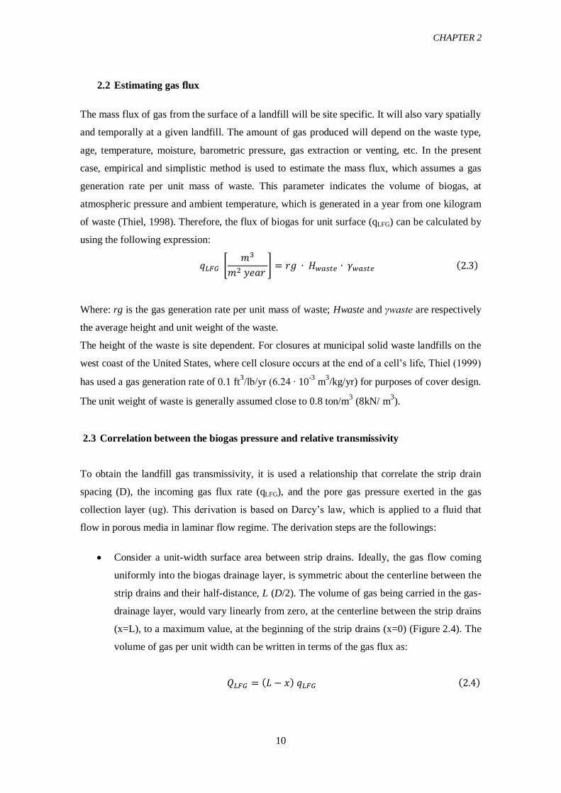
2.2 Estimating gas flux
The mass flux of gas from the surface of a landfill will be site specific. It will also vary spatially
and temporally at a given landfill. The amount of gas produced will depend on the waste type,
age, temperature, moisture, barometric pressure, gas extraction or venting, etc. In the present
case, empirical and simplistic method is used to estimate the mass flux, which assumes a gas
generation rate per unit mass of waste. This parameter indicates the volume of biogas, at
atmospheric pressure and ambient temperature, which is generated in a year from one kilogram
of waste (Thiel, 1998). Therefore, the flux of biogas for unit surface (qLFG) can be calculated by
using the following expression:
𝑞𝐿𝐹𝐺 [𝑚3
𝑚2 𝑦𝑒𝑎𝑟 ] = 𝑟𝑔 ∙ 𝐻𝑤𝑎𝑠𝑡𝑒 ∙ 𝛾𝑤𝑎𝑠𝑡𝑒 (2.3)
Where: rg is the gas generation rate per unit mass of waste; Hwaste and γwaste are respectively
the average height and unit weight of the waste.
The height of the waste is site dependent. For closures at municipal solid waste landfills on the
west coast of the United States, where cell closure occurs at the end of a cell’s life, Thiel (1999)
has used a gas generation rate of 0.1 ft3/lb/yr (6.24 ∙ 10
-3 m
3/kg/yr) for purposes of cover design.
The unit weight of waste is generally assumed close to 0.8 ton/m3 (8kN/ m
3).
2.3 Correlation between the biogas pressure and relative transmissivity
To obtain the landfill gas transmissivity, it is used a relationship that correlate the strip drain
spacing (D), the incoming gas flux rate (qLFG), and the pore gas pressure exerted in the gas
collection layer (ug). This derivation is based on Darcy’s law, which is applied to a fluid that
flow in porous media in laminar flow regime. The derivation steps are the followings:
Consider a unit-width surface area between strip drains. Ideally, the gas flow coming
uniformly into the biogas drainage layer, is symmetric about the centerline between the
strip drains and their half-distance, L (D/2). The volume of gas being carried in the gas-
drainage layer, would vary linearly from zero, at the centerline between the strip drains
(x=L), to a maximum value, at the beginning of the strip drains (x=0) (Figure 2.4). The
volume of gas per unit width can be written in terms of the gas flux as:
𝑄𝐿𝐹𝐺 = (𝐿 − 𝑥) 𝑞𝐿𝐹𝐺 (2.4)

CHAPTER 2
11
Where QLFG is gas discharge flow rate per unit width at any point x in the gas-drainage
layer, L half distance between the strip drains, qLFG flux of biogas for unit cover
surface, (L-x) a unit-width surface area between strip drains.
The flow in the gas-drainage layer can be assumed to follow Darcy’s law (1856), which
can be written in terms of the pressure gradient as follows:
𝑄𝐿𝐹𝐺(𝑥) = (𝑘𝑔
𝛾𝑔) ∙ 𝐴 ∙ (
𝑑𝑢
𝑑𝑥) = (
𝑘𝑔
𝛾𝑔) ∙ (𝑡 ∙ 1) ∙ (
𝑑𝑢
𝑑𝑥) =
= (𝑘𝑔 ∙ 𝑡
𝛾𝑔) ∙ (
𝑑𝑢
𝑑𝑥) = (
𝜓𝑔
𝛾𝑔) ∙ (
𝑑𝑢
𝑑𝑥) (2.5)
Where: kg, landfill gas permeability of the gas-drainage layer; γg, the gas unit weight;
A, cross-sectional flow or area which is obtained by the thickness of the layer (t) times
unit-width; and du/dx is the pressure gradient and ψg, the landfill gas transmissivity.
Combining the relationship (2.4), (2.5) and solving the differential equation for x=0 and x=L,
corresponding respectively to the minimum and maximum gas pressure, the transmissivity of
the gas drainage layer can be obtained by the following expression:
𝜓𝐿𝐹𝐺 =𝑞𝐿𝐹𝐺 ∙ 𝛾𝑔
𝑢𝑔, 𝑚𝑎𝑥 ∙
𝐿2
2 (2.6)
Where: ΨLFG landfill gas transmissivity; qLFG gas flux per unit surface obtained by using the
Thiel (1998) empirical method; L half spacing between the strip drains; γg the unit weight of the
landfill gas; Ug,max the maximum allowable landfill gas pressure obtained fixing minimum
safety of factor.
Figure2.4: Diagram of strip drains operation, placed in the biogas drainage layer (R.Thiel, 1998).

CHAPTER 2
12
2.3 Correlation between biogas and the hydraulic conductivity
To correlate biogas transmissivity and the hydraulic conductivity, it is used the Darcy’s low
(1856) in terms of intrinsic permeability, characteristic of the medium in question. Recalling
equation (2.5), the flow rate for a specific fluid in a porous medium is:
𝑄 = 𝐾 ∙𝛾𝑓
𝜇𝑓 ∙ 𝑖𝑓 ∙ 𝐴 ( 2.7)
Where: Q flow rate; K intrinsic permeability; γf unit weight of the fluid; μf dynamic viscosity of
the fluid; if or dh/dx the fluid gradient, and A cross-sectional area of the flow medium.
The relationship between the standard civil engineering coefficient of permeability (i.e.
hydraulic conductivity) and the intrinsic permeability ,can be written as:
𝑘𝑓 = 𝐾 ∙𝛾𝑓
𝜇𝑓 (2.8)
Where: kf standard civil engineering coefficient of permeability for a given fluid and, K intrinsic
permeability.
Since K is a constant factor dependent on the medium, the ratio between the coefficients of
permeability for two different fluids can be determined as:
𝑘1
𝑘2=
𝜇2
𝜇1 ∙
𝛾1
𝛾2 (2.9)
Where: ki is the standard civil engineering coefficient of permeability of a given fluid, μi is the
dynamic viscosity of the fluid, and γi is the unit weight of the fluid.
This relationship is obtained by using the Darcy equation (1856) and assuming that the same
porous medium is crossed by two different fluids. In the present case, they are biogas and water
(Thiel,1998). Using the previous equation, the design of a biogas drainage layer can now be
accomplished by converting the required gas transmissivity into a required hydraulic (water)
permeability as follow:
𝜓𝐻2𝑂 = 𝜇𝐿𝐹𝐺
𝜇𝐻2𝑂 ∙
𝛾𝐿𝐹𝐺
𝛾𝐻2𝑂 ∙ 𝜓𝐿𝐹𝐺 (2.10)
Where: ΨLFG gas transmissivity of the biogas drainage layer; ΨH2O transmissivity of the water;
γi, unit weight of a give fluid; μi, kinematic viscosity of a given fluid.
2.4 Correlation between hydraulic conductivity and particle size
Hydraulic conductivity (kf) can be estimated by particle size analysis of the interest sediment,
using empirical equations. Some authors summarized several empirical methods from former
studies, presenting the following general formula (Justine Odong, 2013):

CHAPTER 2
13
𝑘𝑓 = 𝑔
𝜐 ∙ 𝐶 ∙ 𝑓(𝑛) ∙ 𝑑𝑒2 (2.11)
Where: kf, hydraulic conductivity; g, acceleration due to gravity; v, kinematic viscosity; C,
sorting coefficient; f(n), porosity function, and de, effective grain diameter. The kinematic
viscosity (v) is related to dynamic viscosity (μ) and the fluid (water) density (ρ).
In the present case, the equivalent diameter of the medium in question is determined using a
relationships, that does not include the parameters characteristic of the soil, like the Hazen
(1892) formula:
𝑘𝑓 = 100 ∙ 𝑑102 (2.12)
Where: kf, is hydraulic conductivity in [cm/s]; d10, effective grain diameter represents the
diameter in [cm] corresponding to a percentage in weight of 10% that is lower than, and 100 is
the sorting coefficient. For applying this relationship, the effective diameter is in the range of
0.1 and 30 mm.
2.5 Determination of biogas transmissivity and hydraulic conductivity of the biogas
drainage layer for the Torretta landfill case study
In the considered case study, the landfill final cover will be realized in accordance with existing
legislation and, providing highly permeable strip drains within the gas collection layer as a
preventive measure to avoid excess of pore gas pressure. Consequently, to obtain the biogas
transmissivity it will be possible to apply the procedure proposed by Thiel (1998).
Applying equation (2.2), it is possible to obtain a linear relationship between the factor of safety
(FS) and the biogas pressure (ug). In the present case, the maximum inclination of the cover is
1:2.5 (Table 2.2).
Table 2.2: Characteristic of the slope.
Slope characteristic
slope 1:2,5
Inclination 40% β 21.8°
cos β 0.93
sen β 0.37
The total thickness (d) of the layers placed above the sliding surface is equal to 2.2 m, as shown
in table (2.3). The average unit weight of the strata above the biogas drainage layer is assumed
equal to 16 kN/m3.
CHAPTER 2
14
Table 2.3: thickness of the layers forming the Torretta landfill final cover.
thickness d [m]
Surface layer 0,44
Protection layer 0,66 Drainage layer 0,55
Clay barrier 0,55
TOTAL 2,20
Figure 2.5: Schematic representation of the slice analyzed for the limit equilibrium limit.
At the lower interface of the hydraulic barrier to prevent clogging phenomena is placed a
geosynthetic layer, capable of exerting the separation function. Therefore, the effective friction
parameter between it and the biogas drainage, is determined through a reference TENAX
catalog and it is assumed close to 30° (Figure 2.6). From a conservative point of view, the
effective adhesion parameter is neglected. Hence, using all these values, it is possible to obtain a
liner relationship between the factor of safety (FS) and the pressure of the biogas (ug), as:
𝐹𝑆 = 1.44 − 0.048 𝑢𝑔 (2.14)
When the pressure of the biogas is zero, in the absence of flow, the factor of safety is equal to
1.44. In agreement with the D.M. 11/03/1988, the slope stability is verified when the safety
factor must be equal or greater than 1.3. According to this value, the maximum allowable
pressure calculated by the proposed Thiel methodology is (Ug,max) 3.2 kPa.

CHAPTER 2
15
Figure 2.6 : Tenax chart.
Figure 2.7: Trend between the factor of safety (FS) and the biogas pressure (ug): for FS equal to 1.3 the
maximum allowable pressure 3.2 kPa.
By using the maximum allowable pressure and equation (2.6), it is possible to obtain the biogas
transmissivity. However, before starting with this calculation, it is necessary to estimate the
mass gas flux from the surface of landfill. For this purpose it is used the empirical relationship
proposed by Thiel (1998), and
Assuming a gas generation rate equal to 6.24 ∙ 10-3
m3/kg/year, an average waste unit weight of
800 kg/m3 and a height of the waste close to 20 m, the landfill gas flow for unit area is equal to
99.84 m3/m
2/year (3.16E-06 m
3 / m
2/ sec).
y = -0.0442x + 1.4434
0.0
0.2
0.4
0.6
0.8
1.0
1.2
1.4
1.6
0 5 10 15 20 25 30 35
FS
ug (kPa)

CHAPTER 2
16
In the present configuration, the vent system is composed by vertical wells placed at a distance
of 25m. Taking into account that the strip drains are connected to them in order to have a single
outlet point, the spacing will be the same. Then, using this parameter, the biogas flow, the half
distance between strip drains and applying the equations 2.6, it is obtained a biogas
transmissivity of 9.752 E-07 m2/s. This value is effective: allows the biogas flow in the porous
medium in theoretical conditions. However, it should be noted that, between the reality and the
schematic operational conditions there are some elements that tend to affect the transmissivity
of the porous medium. For this reason, it is necessary to introduce a design transmissivity,
obtained by increasing the effective one with a series of safety coefficients using the following
expression:
ψLFG,design = ψLFG,calc · FS ·RFin ·RFcr ·RFcc ·RFbc RFbc (2.15)
where ψLFG,calc represents the calculated transmissivity, and the ψLFG,design the design
transmissivity incremented by the following parameters:
FS is the global safety factor that evaluates the uncertainties of the model used;
RFin is a factor that evaluates the reduction to intrusion;
RFcr is a reduction factor that considers creep;
RFcc is a reduction factor for chemical intrusion;
RFbc is a factor reduction to biological clogging.
Table 2.4: Factor of safety adopted in function of their range of variation.
Range of variation Adopted
FS 2,0 ÷ 3,0 3,0
RFin 1,0 ÷ 1,2 1,1
RFcr 1,1 ÷ 1,4 1,1
RFcc 1,0 ÷ 1,2 1,1
RFbc 1,2 ÷ 1,5 1,2
The maximum and minimum factors of safety are respectively equal to 2,64 (FStot,min) and
9,072 (FStot,max). In the present case are assumed the average values, except for the creep and
the uncertainty of the model (Table 2.4). Indeed, for the first is used the lower limit because the
layer is formed from granular material, while for the second it is assumed its maximum value.
In this way, the FS adopted (FStot,design) is equal to 4,792. Multiplying these coefficients for
the prior biogas effective transmissivity, it is obtained the following design value: 2.57E-06
m2/s for the minimum safety factor, 8.85E-06 m
2/s for maximum and 4.67E-06 m
2 /s for the
reference (figure 2.8).

CHAPTER 2
17
Figure 2.8 : Calculated and design biogas transmissivity ψLFG in function of the factor of safety (FS) and the
biogas pressure exerted by the biogas (ug): for FS equal to 1.3, ug is equal to 3.2 kPa and the reference
transmissivity is equal to 4.67E-06 m2 /s.
To convert into water transmissivity the biogas one, is used the expression (2.9). It is assumed
that the biogas is composed by 45% of carbon dioxide and 55% of methane. By using these
percentage, the unit weight of the biogas is equal to 12.8 N/m3. The kinematic and dynamic
viscosity of the fluid in exam are evaluated at atmospheric pressure and with a temperature
equal to 20°.
Tabella2.5: Characteristic parameters of fluid at atmospheric pressure and with a temperature equal to 20°.
Density
(𝝆) [kg/m3]
Unit weight
(𝜸) [N/m3]
dynamic
viscosity (𝝁) [N∙s/m2]
kynematic
viscosity (ν) [m2/s]
Water 1000 9800 1,01∙10-3 1,01∙10-6
Air 1,28 11,8 1,79∙10-5 1,75∙10-5
Carbon dioxide 1,83 17,9 1,50∙10-5 8,21∙10-6 Methane 0,67 6,54 1,10∙10-5 1,65∙10-5
LFG (45% CH4 - 55% CO2) 1,31 12,8 1,32∙10-5 1,01∙10-5
According the parameters reported in the table 2.5, the relationship between the biogas (ΨLFG)
and water transmissivity (ΨH2O) is the following (Muskat,1937):
𝜓𝐻2𝑂 = 1,32 ∙ 10^(−5)
1,01 ∙ 10^(−3) ∙
12.8
9800 ∙ 𝜓𝐿𝐹𝐺 = 10 𝜓𝐿𝐹𝐺 (2.16)
0.0E+00
5.0E-06
1.0E-05
1.5E-05
2.0E-05
2.5E-05
3.0E-05
3.5E-05
0
5
10
15
20
25
30
35
0.0 0.5 1.0 1.5
ψlf
g[m
2/s
]
Ug [
kP
a]
FS
Ug[ kN/m2] ψLFG calc [m2/s]
ψLFGdesign min [m2/s] ψLFGdesign adopted [m2/s]
ψLFGdesign max[m2/s]

CHAPTER 2
18
In accordance with the actual regulation, the thickness of the biogas drainage layer or, in this
case of the transmission component, is equal to 55 cm. Consequently, the hydraulic conductivity
must be higher than 5.15E-05 m/s in the case of FS minimum, 1.77E-04 m/s for the FS
maximum and 9.35E-05 m/s for the FS adopted (figure 2.9). These values are the minimum
allowable. Hence, in order to avoid excess of pore gas pressure, the hydraulic conductivity of
the gas collection layer must be higher than 10-4
m/s. According to this results, a coarse sand
material can be suitable for the biogas drainage layer (Figure 2.10).
Figure 2.9 : Hydraulic conductivity KH2O of the biogas drainage layer in function of the factor of safety (FS)
and the biogas pressure exerted by the biogas: for FS equal to 1.3, Ug is 3.2 kPa and the reference KH2O is
equal to 9.35-05 m /s.
Figure 2.10: Range of variation of the hydraulic conductivity in grain size and grain size distribution
(Algamir,2005).
0.0E+00
1.0E-04
2.0E-04
3.0E-04
4.0E-04
5.0E-04
6.0E-04
7.0E-04
0
5
10
15
20
25
30
35
0.0 0.5 1.0 1.5
KH
20
[m
/s]
Ug
[k
Pa]
FS
Ug[ kN/m2] KH2Omin(m/s) KH2O adottato(m/s) KH2Omax(m/s)

CHAPTER 2
19
As reported in section (2.4), the Darcy law is used (1856) to obtain the correlation between the
hydraulic conductivity of two fluids, which results to be valid only in laminar flow regime. To
verify it is determined the number of Reynold. For sands, the motion is laminar if the Reynolds
number should be less than 10 (Richardson, Thao, 2000):
𝑅𝑒 = 𝜌 ∙ 𝑣 ∙ 𝑑
𝜇𝑓 =
𝑣 ∙ 𝑑
𝜐 (2.17)
Where: ρ represents the fluid density, ν kinematic viscosity µ dynamic viscosity and v the fluid
velocity and d the characteristic size of the surface through which the flow takes place.
Using the values of the biogas flow and the parameters listed in Table 2.5, it is possible to
obtain a Reynolds number equal to 3.9, lower than 10 and therefore in laminar flow regime.
In order to determine the equivalent diameter associated to these hydraulic conductivity is used
the Hazen formula (1892), reported in the section 2.5, and the results obtained is reported in
table 2.7.
Table 2.7: Minimum effective diameter (d10) in function of the hydraulic conductivity obtained.
kf [m/s] d10 [mm]
5.15E-05 0.07
1.77E-04 0.13
9.35E-05 0.1

CHAPTER 3
20
CHAPTER 3: Determination of the grain size distribution of
the biogas drainage layer
In accordance with Legislative Decree 36/2003, the biogas drainage layer must be protected
from clogging (section 1.2). Therefore, shall be placed a separation material at the interface
between the hydraulic barrier and the gas collection layer. In this way, the eroded particles
induced by vibrations and seepage do not alter the hydraulic conductivity of the granular
material forming the layer in question which, as shown in the chapter 2, is determined by the
estimated biogas flow. To determine if this material has particle size distribution compatible
with the underlying layers, it is used filter design criteria. In this way, and through the
knowledge of the particle size of the underlying waste and foundation layer, it will be possible
to define the grain size distribution of the biogas drainage layer.
3.1 General information about filters
In the geotechnical engineering, filters are layers of materials having grains and voids
sufficiently large to allow the passage of water and, small enough to prevent the migrations of
fines particles through the interstices formed by the grains. They are used to prevent problems
like piping and erosion and in many situations in which hydraulic gradients is very high; thus
they are placed at the interface between coarse and fines materials and, in contact with surfaces
that have different particle size.
Filters can be made of natural or synthetic materials. The latters, although capable of exerting
the same properties of granular materials, has a limited durability, which can be accelerated in
aggressive environments such as in a landfill. For these reasons, the synthetic filters are used in

CHAPTER 3
21
situations where it is necessary to protect the material from possible occlusions. There are
multiple models in the literature able to assess in detailed the design of the filter. In the interest
of brevity it is used the simplest empirical models.
3.1.1 Filters of granular materials
This type of filters are generally characterized by granular material, like sand and gravel. The
problems that arise in contact between two materials of different grain size, affected by seepage
oriented towards the coarse-grained material and having high hydraulic gradient at the transition
from one to another material, are two limit state conditions, defined as:
Clogging: occurs when the pores of coarse material are gradually occluded by the
particles of the finer material, until preclude its hydraulic efficiency (Figure 3.1 a);
Erosion: occurs when the finer particles of the basic material completely pass through
the pores of the coarse material. This phenomenon causes a progressive erosion of the
base medium that can evolve to the formation of pipes inside the base material able to
adversely affect the stability of the work (Figure 3.1 b);
The filters collapse when they are reached this limit state conditions (Moraci et. al., 1996). The
design of a transition zone, in the literature conventionally known as filter, has the aim to deal
with clogging and erosion conditions limit.
Figure 3.1: a) clogging; b) erosion (Colombo e Colleselli).

CHAPTER 3
22
To prevent the limit state reported above, it is necessary to satisfy the following filter design
criteria:
Clogging criterion: the material forming the filter must be fine enough to prevent the
adjacent finer material from piping or migrating into the filter material;
Permeability criterion: the filer material must be coarse enough to carry water without
any significant resistance;
Internal stability criterion: the filter material must be stable, it means that the local
particle size composition and permeability ,under the drag action exerted by the fluid,
must be preserve in order to do not suffer appreciable variation in time.
These design criteria are performed in order to evaluate the filter efficiency starting from the
grain size distribution of the material. Indeed, most of the methods used in the design of filters
formed by granular materials, is in function of the geometrical characteristics of the two
materials that interact in the phenomenon.
The particle size distribution represents a curve in which grain size of the material is reported
along the bottom and, the percent of a soil that is smaller than (“or passes”) each dimension is
shown on the left side. This type of analysis is performed by using standard sieves, sized
according to standard classification system. Obtained this curve, the material is described by
parameters, which are (Harold N. Atkins):
Uniform coefficient (Cu): this value gives an indication of the shape of the curve and
the range of particle sizes that a soil contains, especially in the more important fine
part of the soil. Uniform coefficient is expressed as:
𝐶𝑢 = 𝑑60
𝑑10 (3.1)
Where d60 and d10 are the grain size that only 60% and 10% of the grains are finer
than. A material is uniform when the Cu is equal to 2, poor graded when Cu is lower
than 6, well graded when Cu is higher than 15;
Coefficient of curvature (Cc): this is another measurement of the shape of the curve.
𝐶𝑐 = 𝑑302
𝑑60 𝑑10 (3.2)
Where d60,d30 and d10 are the grain size that only 60%, 30% and 10% of the grains
are finer than.

CHAPTER 3
23
3.1.2 Filters of synthetic materials
The filters of synthetic material were born with geosynthetic materials produced by the plastics
and textiles industries. This category belong to nonwoven and woven geotextiles, which usually
perform a filtering and separation function.
The limit states faced by these types of filters are the same seen for granular material, with the
addition to the blinding limit state: the filter of geosynthetic material must be able to avoid
accumulation of fine particles on the geotextile surface and hence, the formation of a low
permeability zone which can increase pore pressure. For synthetic filter the internal stability
criterion loses meaning, while clogging and permeability still have to be verified.
Figure 3.2: Blinding and clogging limit state (Colombo e Colleselli).
3.2 An empirical method for evaluating the grain size compatibility
The particle size compatibility are verified when permeability and clogging criterion is satisfied.
In other words, the base material must have voids small enough to retain filter particles, and
sufficiently large to allow the flow. Erosion and occlusion in a filter depends on different
variables, often uncertain and difficult to quantify (Ruot, 2006). Consequently, is employed
empirical or probabilistic models in order to verify the particle size compatibility, which are
based on the dimensions, geometry and gradation of the material used. In the present case, for
satisfying this criterion, is used the model proposed by Terzaghi (1922). This is empirical and
bases on the grain size distribution curve of the material (figure 3.3).
Considering two materials placed in contact with each other, the clogging criterion wants to
avoid the erosion of fine particles. For this purpose, the method proposed by Terzaghi compares
the coarse fraction of the base material (d85b), with the fine fraction of the filter material (d15f):
𝑑15 𝑓
𝑑85 𝑏 < 4 (3.3)
Where d15f and d85b are the grain size corresponding to 15 and 85% passing, respectively, and
can be obtained from the grain size curves of each material.

CHAPTER 3
24
Figure 3.3 : Graphical representation of the Terzaghi methodology (1922) (Colombo e Colleselli).
This criterion should be applied not only to the filter material but also to the drainage layer. This
will prevent migration of the subgrade material into the sub-base and the sub-base into the
drainage layer.
The permeability criterion, instead, is formulated in order to avoid excess of pore water
pressure. The permeability of the two materials must increase in the flow direction for allowing
the flow (Graauw et al., 1984). Therefore, the filter must be maintained at least an order of
magnitude higher than that of the base material (Moraci et al., 1996). The method proposed by
Terzaghi compares the fine fraction of the base material (d15b), with the fine fraction of the
filter material (D15f):
𝑑15 𝑓
𝑑15 𝑏 > 4 (3.4)
In which d15 is the grain size corresponding to 15% passing. This criteria need to be applied
only to the filter or the sub-base. The drainage layer is so permeable and this criterion can
certainly be satisfied.
3.3 An empirical method for evaluating the internal stability of the material
Material is defined internally stable when its skeleton does not affect modification. When finer
soil particles (mobile particles) are moved through constrictions between larger soil particles
(soil skeleton) by hydraulic or seepage forces, the material are considered unstable. In literature,
this is described as suffusion (Chapuis, 1992). Usually, internally unstable material are those
broadly graded soils with particles from silt or clay to gravel size, whose particle size
distribution curves are concave upward, or gap graded soils (Wan e Fell, 2008). However, even
materials which have a uniform particle size distribution curve can be internally unstable.

CHAPTER 3
25
Figure 3.4: Grain size distribution curve: uniform, well graded and e gap graded; (Yun Zhou, 1998).
To assess the internal stability of a layer formed from granular material, there are several
empirical methods. Among the many, it is focused the Kezdi (1979) and Kenney and Lau
(1985) approach.
Kezdi (1979) proposed splitting up the grain size distribution of a soil into two distributions of
the fine and coarse parts, and assessing the stability by Terzaghi’s well-known filter criterion
applied to the two distributions:
𝑑15 𝑓
𝑑85 𝑏 < 4 𝑓𝑜𝑟 𝑒𝑎𝑐ℎ 𝑑 ∗ (3.5)
Where d15f grain diameter for which 15% of the grains by weight of the coarse soil are smaller;
and d85b grain diameter for which 85% of the grains by weight of the fine soil are smaller; d* is
a generic grain size by which the curve of the tested material is cutting.
Figure 3.5 : Graphical interpretation of the Kezdi (1979) method (Musso e Federico,1983) .

CHAPTER 3
26
Kenney and Lau (1985) proposed transforming the ordinary grain size distribution curve to a F-
H diagram. Here F is the mass percentage of grains with diameters less than a particular grain
diameter d and H is the mass percentage of grains with diameters between d and 4d. The soil
will be considered as stable if, for F< 20 or 30% the curve thus obtained is located above the
critical line H=F. On the contrary, if some portion of this curve passes below the line H=F, the
soil will be considered as unstable. According to Kenney and Lau (1986) the values of 20%
applies to the widely graded soil in the range 0.2< F<1 and the values of 30% to the normally
graded soils in the range of 0.3< F< 1.
Figure 3.6: Graphical interpretation of the Kenney e Lau method (1986).
3.4 Grain size distribution curve of the biogas drainage layer
In accordance with the filter design criteria, reported in the section 3.2 and 3.3, the grain size
distribution curve of the biogas drainage layer must be internally stable and compatible with the
neighboring layers. The presence of a non-woven geotextile at the interface with the clay,
allows us to exclude the upper layers from the calculations subsequently proposed. Therefore, to
identify the curve in question, we will proceed by applying the Terzaghi (1922) empirical
methods and considering as base materials the underlying waste. Contextually is identified the
particle size distribution of the foundation layer, because it is placed between the biogas drain
and waste (paragraph 1.2).
3.4.1 Grain size distribution of the municipal solid waste
Municipal solid waste (MSW) is a mixture of wastes that are primarily of residential and
commercial origin. Typically, they consist of: organic waste, paper, fabric, garden wastes,
plastic, pieces of metal, rubber, glass, waste from demolition, slag and ash. The proportion of

CHAPTER 3
27
these materials will vary from one site to another and also within a site. Life style changes,
legislation, seasonal factors, pre-treatment and recycling activities result in a changing waste
stream over time. Moreover, the composition of MSW varies from region to region and country
to country (Dixon, 2004).
The particle size of the wastes are reduced over time due to the degradation processes that occur
within the landfill. Therefore, the composition of the waste is identified as a function of the
degree of aging (Figure 3.7). Consequently, because of their great variability is assigned them
an area that describe the grain size distribution curve built on a semi-logarithmic plane, which
varies from silt or clay to gravel size. A fresh MSW whose fill age is less than a few years
would contain significant amounts of organic components with size larger than gravel (Hyun Il,
Borinara and Hong, 2011). Grain size distribution of the waste presents a uniform coefficient
higher than 15, and then is considered well graded.
In the present case, wastes represent the base material. Then, for the filter design criteria, it is
used the lower limit of the area that characterize the dimension of this material: the particles
migration due to erosion is oriented toward the voids created by coarse particles forming the
waste from clogging criterion.
Figure 3.7: Grain size distribution curve of the municipal solid waste from Jessberger (1994); (Hyun Il,
Borinara and Hong, 2011).

CHAPTER 3
28
3.4.2 Grain size distribution and internal stability of the foundation layer
As described in section 3.2 and 3.3, the grain size distribution curve of the foundation layer
must be internally stable and compatible with the underlying waste. To prevent migration
phenomena of fine particles forming this layer, it is necessary to apply the Terzaghi’s clogging
criterion. According to this method, the d15 of waste is approximately equal to 16 mm and
hence, the d85 of the foundation layer must be greater than 4 mm, as shown in figure 3.7.
Applying the Terzaghi’s permeability criterion, the d15 of the foundation layer should be less
than 4mm. However, these layers are dry and not crossed by a water flow, then the use of this
principle is only conservative.
In agreement with these observations, it is determined an indicative grain size distribution
curve, that has d15 and d85 respectively equal to 4 and 20 mm (figure 3.8). It has an upwards
concavity, is uniform and has no gaps, in other words, and according to the definitions reported
in the section 3.3, is internally stable (Figure 3.9 e 3.10). Based on these results, the suitable
material for the foundation layer consists of gravels.
Figure 3.8: Graphical representations of the grain size distribution (GSD) of the foundation layer, compared
whit the GSD of the waste material.
0
10
20
30
40
50
60
70
80
90
100
1 10 100 1000
p(%
)
d [mm]
GSD waste GSD foundation layer

CHAPTER 3
29
Figure 3.9: Internal stability results of the foundation layer obtained by using Kezdi procedure (1979);
Figure 3.10: Internal stability results of the foundation layer obtained by using Kenney e Lau procedure
(1986);
3.4.3 Grain size distribution and internal stability of the biogas drainage layer
Through the Thiel’s procedure (1998), and the Hazen’s formula (1892) it was possible to
identify the minimum equivalent diameter (d10) of the biogas drainage layer (section 2.6). In
particular, it must be greater than 0.1 mm and, in the present case, it represents an additional
information by which it is possible to determine the grain size distribution curve of the biogas
drainage layer.
0
0.5
1
1.5
2
2.5
3
1 10 100
d15/d
85
d*[mm]
0
0.1
0.2
0.3
0.4
0.5
0.6
0.7
0 0.2 0.4 0.6
H
F

CHAPTER 3
30
Applying the Terzaghi’s clogging criterion (section 3.2) and considering the worst case
scenario, foundation layer formed by material that is homogeneous, uniform (Cu ≤ 2) and of
size equal to 4 mm (section 3.4.2), the d85 of the drainage layer of the biogas should be greater
than 1mm. This hypothesis is considered conservative and therefore applicable.
An example of the grain size distribution curves of the three layers is reported in figure 3.11.
They identify the minimum order of magnitude of the material used. Indeed, as reported
previously, the d85 of the foundation and biogas drainage layer, are respectively equal to 1 mm
and 4 mm. Moreover, according to the definitions reported in the section 3.3, the curve of the
biogas drainage layer is internally stable, as it shown in figure 3.12 and 3.13. Based on these
results, the suitable material for the biogas drainage consists of coarse sand.
Figure 3.11: Graphical representations of the minimum grain size distribution (GSD) of the biogas drainage
layer, compared whit the GSD of the waste and the foundation layer.
0
10
20
30
40
50
60
70
80
90
100
0.01 0.1 1 10 100 1000
p(%
)
d [mm]
GSD waste GSD foundation layer GSD drainage layer

CHAPTER 3
31
Figure 3.12: Internal stability results of the biogas drainage layer obtained by Kezdi procedure (1969);
Figure 3.13: Internal stability results of the biogas drainage layer obtained by Kenney e Lau procedure
(1985);
0
0.5
1
1.5
2
2.5
3
3.5
0.01 0.1 1 10
d15/d
85
d* [mm]
0
0.1
0.2
0.3
0.4
0.5
0.6
0.7
0 0.2 0.4 0.6
H
F

CHAPTER 4
32
CHAPTER 4: Analysis of the loads acting on the biogas
drainage layer
The actions present on the biogas drainage layer are different and classified in two main
categories:
Permanent, explicated throughout the entire useful life of the work:
- static load induced by weight of the upper layers.
Variable, presents during its installation:
- due to vehicles used for the installation of the biogas drainage layer;
- due to the energy transmitted by compactions means used for the realization of the
hydraulic barrier.
The task of the granular material forming the biogas drainage layer is to resist to these actions.
4.1 Permanent loads
According to the legislative decree 36/2003, the biogas drainage layer is placed at the base of
the final landfill cover. For this reason, it must bear the weight of the upper layers, that is
considered as a uniformly distributed load, of intensity calculated by the following relationship:
𝑞 [𝑘𝑁
𝑚2] = 𝛾 [
𝑘𝑁
𝑚3] ∙ 𝑠 [𝑚] (4.1)
Where q is the uniformly distributed load or weight for unit surface acting on the strata, γ is the
average unit weight, and s is the thickness of the strata placed above the biogas drainage layer.

CHAPTER 4
33
Table 4.1: characteristics of the layers forming the final landfill cover.
Cover layer Height, h [m] thickness, s [m] γ[kN/m3]
Protection layer 1 1 17
drainage 0.66 1 16.5
Hydraulic barrier 0.55 1 20
Biogas collection layer 0.55 1 16.5
The characteristics parameters of the layers are reported in Table 4.1. For safety reasons, in this
part of the work it is assume an average unit weight of 20 kN/m3. Therefore, the uniformly
permanent load acted on the biogas drainage layer is equal to 20 kPa.
4.2 Variable loads
The operating loads are due to the actions of the vehicles used for the installation and realization
of the biogas drainage layer and, to the energy transmitted by compaction means for the lying of
the hydraulic barrier.
Loads induced by work means
During the realization of the biogas drainage layer, the material used is loaded into trucks,
transported on landfill, tipped, compressed and spread by work means. The effect of these
actions on the material can be translated as resistance to:
- Impacts due to falling;
- Fracturing due to crushing;
- Wear, abrasion and friction due to grains sliding induced by work means.
These dynamic efforts are being very aggressive in respect of the material. Therefore, before the
realization of the biogas drainage layer it is necessary to evaluate their effect.
Loads induced by the compaction of the hydraulic barrier
The third and last type of action is induced by the action transmitted through compaction of the
above hydraulic barrier. In this case, this load is applied on a strata because the biogas drainage
layer has been realized. Therefore, the material is confined and behaves has a continuum
medium.
CHAPTER 4
34
The hydraulic barrier has the aim to minimize and prevent water infiltration into the body waste.
Consequently and in accordance with the legislative decree 36/2003, it must realize by using
clayey or silty-clay material, suitably installed by compaction in order to:
- Decrease permeability;
- Increase shear strength;
- Reduce compressibility;
- Controlling shrinkage and swelling;
- Reduce the potential liquefaction.
The compaction is performed by impressing a certain energy, that depends on type, weight and
power exerted by the means used. In the case of cohesive material is preferable to transmit a
quasi-static load and working with sheep foot roller.
In specific, it means to work at low speed and high energy and pressure. The compaction takes
place for successive layers of 20-30 cm and therefore, the layer in question must be compressed
for determined intervals of time. Moreover, through the grains contact this pressure is
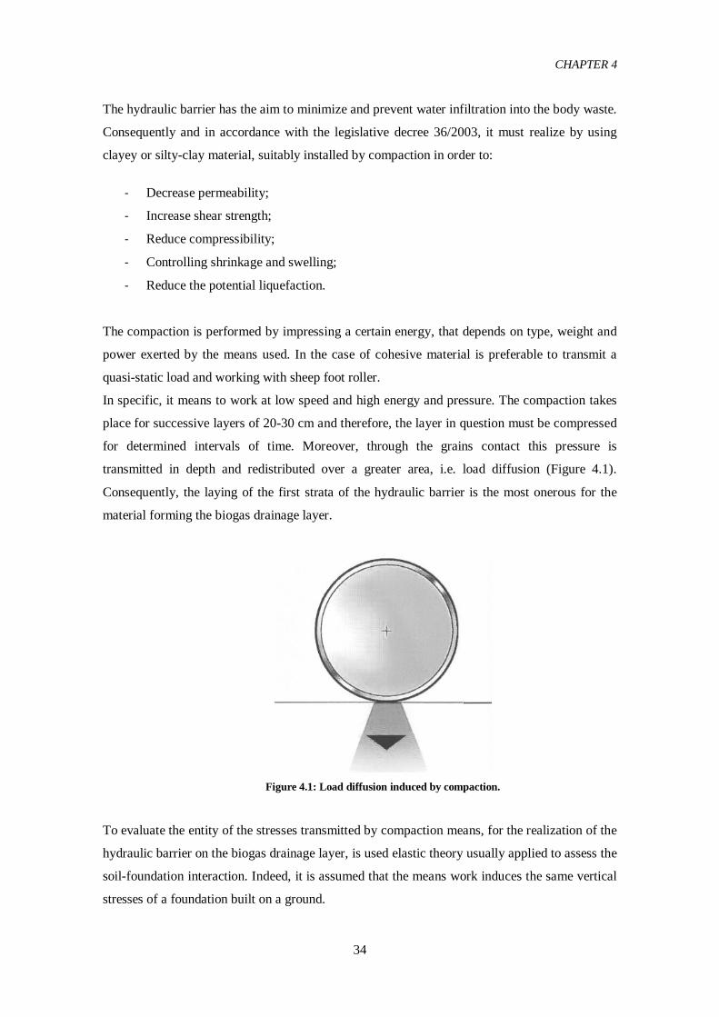
transmitted in depth and redistributed over a greater area, i.e. load diffusion (Figure 4.1).
Consequently, the laying of the first strata of the hydraulic barrier is the most onerous for the
material forming the biogas drainage layer.
Figure 4.1: Load diffusion induced by compaction.
To evaluate the entity of the stresses transmitted by compaction means, for the realization of the
hydraulic barrier on the biogas drainage layer, is used elastic theory usually applied to assess the
soil-foundation interaction. Indeed, it is assumed that the means work induces the same vertical
stresses of a foundation built on a ground.

CHAPTER 4
35
The Boussinesq’s method(1885) was the first used for this type of analysis. Through this model
it is possible to determine the stresses produced by the application of a uniform force P, that acts
perpendicular to an horizontal surface placed on a semi-infinite, homogeneous and isotropic
solid. As said before, the solutions of this method are obtained by the elastic theory: when the
load is removed any type of deformation or settlement produced is reversible.
The equation of the vertical stresses for a point N, located at depth z from the horizontal surface
and at a distance r from the vertical, can be written in polar coordinates as:
𝜎𝑧 = 3𝑃
2𝜋
𝑧3
( 𝑧2 + 𝑟2)52
= 𝑃
𝑧2 𝐼𝜎 (4.2)
Where σz is the vertical stress for a point N, located at depth z from the horizontal surface and,
at distance equal to r from the vertical surface, for a point a of application P (figure 4.2). The Iσ
is the influence factor of vertical force and depends on the point in which you want to know the
stress state.
Figure 4.2: Graphical representation of the Boussinesq model.
In practical applications, it is used charts that are able to identify or provide, for different types
of charged areas, the following data:
The variation of the vertical stress q in function of the depth z, along axis or in the
center of the loading area;
The trend of the curves of equal pressure in a vertical cross section.
These data allow the determination of the vertical stresses distribution on any horizontal
surfaces. In the present case, it is considered the Steinbrenner (1934) solution for a rectangular

CHAPTER 4
36
footprint loading, which is representative of the pressure transmitted by the compactions means.
For simplicity it is used the reference chart, through which it is possible to determine the
vertical stress present at 30 cm depth (thickness of the first strata forming the hydraulic barrier)
from the biogas drainage layer. To proceed with this calculation it is necessary to evaluate the
pressure transmitted by the work means (q) and the dimension of the sheep foot roller footprint,
width (L) and thickness (B). Through these values it is possible to enter in the references
Steinbrenner (1934) chart, which is shown in Figure 4.3, and define the pressure transmitted on
the biogas drainage layer.
The most unfavorable loading condition for the biogas drainage layer is obtained when the L/B
ratio tends to infinity and the z/B ratio tends to zero. This assumption is satisfied when the
depth, z, is very small and the load width, L, is very large. Hence, as shown in the table 4.4, the
ratio between the vertical stress (Δσz) and the load (q) is equal to 0.25.
Figure 4.3: Steinbrenner chart (1934);

CHAPTER 4
37
Figure 4.4: Values of ∆σ/q in function of z/B and L/B obtained from the Steinbrenner solution (1934);
Multiplying this value for the pressure applied by the sheep foot roller, it is possible to obtain
the vertical stresses acting on the biogas drainage layer. More specifically, the load for unit
surface transmitted by the compactions means (q) varies between 1400 and 7000 kPa, and
assume an higher value in function of the drum types. Consequently, the vertical stress (σz) is
respectively equal to 350 kPa and 1750 kPa.
4.3 Actions analysis and modes of grain breakage
Considering the results obtained in the previous sections (4.1 and 4.2), the material forming the
biogas drainage layer will be subject, in the following sequence, to:
Fracturing, attrition and wear induced by dynamic efforts due to grains contacts, sliding
and impacts explicated during the installation;
Compression induced by quasi-static load and static load, respectively for the compaction
of the hydraulic barrier and for the weight of the overlying layers.
Table 4.2: Intensity of the static loads.
Load Intensity (kPa)
Permanent 20
Quasi-Static 350-1750
Looking at table 4.2, it is noted that the load induced by the compaction means is more
heavily than the weight transmitted by the overlying layers.

CHAPTER 4
38
It is important to note that , in this case, it is not considered the property called "freezing", or
ability of the layer to withstand frost and freeze-thaw cycles: in our climates the annual heat
wave interests a layer of the order of 60 cm, below which the temperatures does not drop below
0°C. In the present case, the thickness of the layers placed above the biogas drainage layer is
greater than 60 cm, and then the layer itself will never be subject to the above actions.
In each cases, the material can arrive at failure and can change the geotechnical requirements for
which is chosen (sections 2.6 and 3.4). Due to mechanical actions, the grain breakage may
classified according to three modes (Guyon and Troadec, 1994):
Fracture: a grain breaks into smaller grains of similar sizes (i.e. splitting);
Attrition: a grain breaks into one grain of a slightly smaller size and several much
smaller ones;
Abrasion: the result is that the granulometry remains almost constant but with a
production of fine particles (lower than the effective size).
Figure 4.5: Different modes of grain breakage: (a) fracture; (b) attrition; and (c) abrasion (Ali Daouadji
et al, 2001).
Hence, the splitting of grains corresponds to a mode of grain rupture by fracture; the rupture of
sharp angles to the mode of rupture by attrition, whereas the rupture of micro asperities, during
the sliding of grains, corresponds to the mode of rupture by abrasion. The latter may occur in
the absence of notable fracture or attrition; for example, during cyclic tests of small stress
intensity, as in a railroad ballast, for which grain size and grain size distribution do not change
in significant proportion. Fracture and attrition can lead to significant changes in the grading
curve and consequently, the mechanical properties of granular material can significantly change
(Daouadji Ali et al, 2001).
Hence, the correlation between the loads and grain breakage is summarized in Table 4.3.

CHAPTER 4
39
Table 4.3: Correlation between the grain breakage and the associated actions;
Grain Breakage Actions Effect
Fracture Impacts
Compression Lead to significant changes in the grading curve;
Attrition Sliding of the
grains Lead to significant changes in the grading curve;
Abrasion Wear
freeze-thaw Lead to an increment of the fine fraction of the
grading curve;

CHAPTER 5
40
CHAPTER 5: Intrinsic characteristics of granular materials
As explained in Chapter 4, the granular material formed the biogas drainage layer must possess
a mechanical resistance through which withstand static and dynamic loads. Therefore, in this
chapter, in order to define this characteristics will be reported literature studies.
Granular materials are defined as loose materials consisting of a set of discrete particles or
grains including sand, gravel, rocks and aggregate, i.e. granular mineral particles used in
construction or in combinations with various types of cementing material to form concretes or
used alone as road bases, backfill, etc. Usually, they are classified in function of their
dimension. Based on this property, they show different mechanical behavior. According to the
AASTHO classification, are those having dimension higher than 0.075mm (Table 5.1).
Table 5.1: Granular materials classification based on their dimensions; MIT (Massachusetts Institute of
Technology), AASHTO (American Association of State Highway and Transportation Officials), AGI
(Association geotechnical Italian) (Lancelotta, 1983).
System Gravel [mm] Sand[mm] Silt [mm] Clay [mm]
MIT(1931) 60÷2 2÷0.06 0.06÷0.002 <0.002
AASTHO(1970) 75÷2 2÷0.075 0.075÷0.002 <0.002
AGI > 2 2÷0.02 0.02÷0.002 <0.002
CP 2001 (1957) 60÷2 2÷0.06 0.06÷0.002 <0.002

CHAPTER 5
41
The granular material resistance depends on the intrinsic characteristics of individual grains,
such as shape, size, particle size distribution and its mechanical resistance.
Shape
Flat particles, thin particles, or long, needle shaped particles break more easily than cubical
particles (Harold N,Atkins). Increase in grain breakage depends also on the angularity of grains
(shape factor). This may be due to a greater fragility of the contact points of small curvature
radii and to the intensity of forces at contact points (Hardin, 1985; Ali Daouadji et al, 2001).
Size
A bigger grain breaks easily than finer one. (Mitchell,1993; Lee and Farhoomand,1967).
Smaller particles are generated from the larger ones along zones of lower strength. As the
particle size increases, particle crushing also increases. Larger particles contain more flaws or
defects and then, they have a higher probability of the defect being present in the particles that
will break. As the breakdown process continues, there are fewer defects in the subdivided
particles. Therefore, similar particles are less likely to fracture as they become smaller
(Yamamuro and Lade (1996).
Grain size distribution
Lower is the uniform coefficient of the material, higher is the grain breakage. Tested in the same
mechanical conditions and for identical nature parameters except for the value of Cu, the well
graded mixture presented very slight evolution in its grain size distribution in contrast to the
badly graded mixture (Figure 5.1)( Ali Daouadji et al, 2001). Well-graded soils do not break
down as easily as uniform soils. As the relative density increases, the amount of particle
breakage decreases. Both these factors are based on the fact that with more particles
surrounding each particle, the average contact stress tends to decrease (Yamamuro and Lade
(1996). Densely graded aggregate layers also increase the strength developed: particles are
locked together to a greater degree, aiding in the development of frictional resistance to shearing
failures.

CHAPTER 5
42
Figure 5.1: Evaluation of the influence of the uniform coefficient on the grain size distribution for two
different material G1 and G2, having respectively Cu equal to 10 and 2 (Hicher et al.,1995) .
Table 5.1: Tests performed on granular material to determine some properties.
Properties Test
Gradation Sieve analysis
Hardness and Abrasion Aggregates impact test- Los Angeles abrasion test
Aggregates pressure test- Darry abrasion test
Aggregates friction test- Deval abrasion test
Durability Soundness test
Deleterious Substances Petrographic analysis
Sand equivalent test
Fines Content Washed sieve analysis
Particle shape Amount of thin or Elongated particles
Particle surface Amount of crushed particles
Chemical stability Reactivity - stripping
5.1 Definition of grains quality
In addition to the aforementioned parameters, it is important to consider other properties
indicative of the mechanical strength of the material. They are:
Hardness, abrasion or resistance to wear;
Durability;
Surface texture;
Deleterious substances;

CHAPTER 5
43
Crushing strength;
Soft and light weight particles.
They give an indication of quality of the material used.
Hardness, Abrasion or resistance to wear
The hardness and abrasiveness of rocks depend on type and quality of the various constituents
and, by the bonds between them. Hardness is defined as the penetration or deformation
resistance of a body induced by external forces. It is expressed by a number that indicates the
characteristics of the material plastic deformation. It is a concept related to the behavior of the
material, rather than a fundamental property.
Abrasion is the superficial removal of material caused by repeated friction actions. Therefore, it
indicates the ability of the material to resist wear or degradation phenomena. As hardness, it is
associated to the mechanical behavior of the material.
Durability
The durability of an aggregate particle shows its resistance to disintegration due to cycles of
wetting and drying, heating and cooling, and especially freezing and thawing. Aggregates
particles have pores, which often become saturated. Repeated cycles can cause the particles to
break. This is especially dangerous with particles from sedimentary rocks, which usually have
planes of weakness between layers.
Shape and surface texture
Particle shape and surface texture affect the strength of the aggregate particles, the bond with
cementing materials, and the resistance to sliding of one particle over another. Particles with
rough, fractured faces allow a better bond with cements do rounded, smooth gravel particles.
Rough faces on the aggregate particles also allow a higher frictional strength to be developed if
some load would tend to force one particle to slide over an adjacent particle.
Deleterious substances o fines
Deleterious substances are harmful or injurious materials. They include various type of weak or
low-quality particles and coatings that are found on the surface of aggregates particles.
Deleterious substances include organic coating; dust (material passing 0.0075 mms sieve), clay
lumps, shale, coal particles, friable particles, etc. These substances may affect the strength of the

CHAPTER 5
44
aggregate. Soft particles may be unsuitable where they may be exposed to abrasion, such as
road surface.
Crushing strength
Crushing strength is the compressive load that aggregate particles can carry before breaking.
This trait is relatively important for most aggregate uses since aggregate strength of the asphalt
or concrete mixture.
Chemical stability
Chemical stability refers to specific problems due to the chemical composition of aggregate
particles. The presence of material unstable influences the capacity of the material to maintain
its properties.
5.2 Determination of the tests used to determine the mechanical resistance of the
aggregates
The grains or aggregate mechanical resistance is strictly correlated to the parent material. In the
case of natural materials it is a function of the mineralogical composition, whereas for artificial
materials it depends on different factors, like raw material, mixture or chemical component.
Therefore, the history of its natural deposition, or the history of its fabrication for the artificial
mixtures, can be a determining factor (Ali Daouadji et al, 2009).
Generally, an aggregate is a brittle material: achieved the maximum allowable stress arrives at
failure without strain. Then, at some point, the material suddenly collapses or crushes. The grain
o particle mechanical resistance is evaluated by the uniaxial compressive test and calculated as
(Jaeger , 1967):
𝜎 =𝐹
𝑑2 (5.1)
where σf [kPa] is the single particle strength; F is the load at failure and d is the diameter of the
grain (corrected or not from asperity crushing). Thus, as the size of the grains decreases due to
crushing, the strength of the new grains increases (Ali Daouadji et al, 2009).
The mechanical resistance is strictly correlated with parameters such as hardness, durability and
abrasion resistance. Indeed, it increases with the quality of the materials used (Al Harti,2001).
Therefore, to determine this property can be performed laboratory tests, usually applied for
evaluating the friction, wear, impact and crushing resistance. For the first three categories of

CHAPTER 5
45
actions are used the Los Angeles abrasion test. In order to measure the resistance of an
aggregate to crushing, under gradually applied compressive load, are applied the aggregate
crushing test; while for assessing the resistance to sudden shock are performed the aggregate
impact test (Al-Harti,2001). In general, they are used for determining the effects of frictional
and compressive forces induced by pressure applied over the material. However, exist other
tests able to evaluate the quality and the strength of the aggregates, like the Deval and Darry
abrasion tests (Harold N.Atkins,2006).
Despite, they are time consuming and require large quantities of aggregates of specified
grading, they are extremely useful in determining the quality of the aggregates (Al-Harti,2001).
Indeed, aggregate is exposed to a number of physical and chemically degrading forces during
processing, transporting, and construction. They must be tough and abrasion resistant to prevent
crushing, degradation and disintegration when stockpiled, fed through an asphalt plant, placed
with a paver, compacted with rollers, and subjected to traffic loadings. Aggregates, which do
not have adequate toughness and abrasion resistance, may cause construction and performance
problems (Ugur I., et. al. 2010).
The Los Angeles abrasion test, the aggregate impact test and the aggregate crushing test types of
tests are destructive and then, the material modifies irreversible its external surface (Al-Harti,
2001).
The result of these types of test is a bulk index value, that indicates the percentage by weight
retained on a sieve, of size smaller than the dimension of the fraction analyzed. It is determined
by sieve analysis: the mass index is equal to the material passing a sieve of standard dimension
(2.36 or 1.7 mm), that is variable with the considered test ( Table 5.2). A crushing and degraded
material presents values of these index very high (Ugur I., et. al. 2010). Shape, dimension, fine
fraction and grain size distribution can be completely different for a given bulk index obtained
from different materials: the results of these tests does not indicate the way in which the
particles have decreased their size (Stenlid, 1996; Thörnvall, 1997).
Table 5.2: Bulk indexes obtained for different test.
Test Result Material*
Aggregate
impact test 𝐴𝐼𝑉 (%) =
[𝑀𝑖 − 𝑀2.36]
𝑀𝑖 ∙ 100
Retained on sieve 9.52mm
and passing 12.70 mm
Los Angeles
abrasion test 𝐿𝐴 (%) =
[𝑀𝑖 − 𝑀1.7]
𝑀𝑖 ∙ 100
Material retained on sieve of 19 mm
or 7.5 mm
Aggregate
crushing test 𝐴𝐶𝑉 (%) =
[𝑀𝑖 − 𝑀2.36]
𝑀𝑖 ∙ 100
Retained on sieve 9.52mm(or 10mm)
and passing 12.70 mm (or 14mm)
*depend on the classification system

CHAPTER 5
46
5.2.1 Los Angeles Abrasion test
The abrasion tests measure the wear resistance of rocks or aggregates by using an abrasive
material, or for contact with another rock or metal. The result gives an indication of the
hardness, toughness and the quality of the material. Simulates the effect induced by cyclic
loading, freezing and thawing, and evaluates the degradation resistance by wear and abrasion. Is
generally used to test the mechanical resistance of aggregates used for road foundations.
Consequently, simulates the effect of vehicle loads for a time equal to the nominal lifetime of
the work itself.
The Los Angeles test is performed using a sample having dimensions in a well-defined range
and having a weight close to 5000g (Table 5.3). In accordance with the ASTM system,grain size
must be within in one of the ranges reported in Table 5.3; while according to UNI 1097-2, the
sample must be between 10 and 14 mm and also must meet one of the following requirements:
between 60% and 70% passing through a sieve test 12.5mm; or between 30% and 40% passing
through a sieve test by 11.2 mm.
Test samples were oven-dried at 105–110 °C for 24 hours and then cooled to room temperature
before they were tested. After that it is placed in a drum with 11 steel balls (the abrasive charge)
of weight between 400 and 450 grams. The drum was rotated for 500 revolutions at a rate of
30–33 rev/min and then the sample was sieved through the No. 12 sieve (1.7 mm). The amount
of material passing the sieve, expressed as a percentage of the original weight, is the LA
abrasion loss or percentage loss.
𝐿𝐴 (%) = [𝑀𝑖 − 𝑀1.7]
𝑀𝑖 ∙ 100 (5.2)
Mi represents the initial mass, Mf the mass retained on a sieve of 1.7 mm.
Table 5.3: The grain size composition of the sample for coarse aggregates smaller than 38 mm (ASTM).
Size- in square mesh sieve (mm)
Weight classes in grams- Grain size composition
Passing Retained A B C D
38 25.4 1250±25 - -
25.4 19 1250±25 - -
19 13.2 1250±10 2500±10 -
13.2 9.5 1250±10 2500±10 -
9.5 5.6 - - 2500±10
5.6 4.7 - - 2500±10
4.7 2.3 - - - 5000±10
Total 5000±10 5000±10 5000±10 5000±10

CHAPTER 5
47
Figure 5.2: Los Angeles apparatus (ISRM,1998).
5.2.2 Aggregate impact test
Aggregate impact test is used to evaluate the resistance of the aggregate when subjected to a
sequence of impact. The apparatus consists of a steel test mould with a falling hammer or
weight as shown in Figure 5.3. The material used is aggregate passing a 12.70 mm sieve and
retained on a 9.52 mm sieve. It shall be clean and dry (washed if necessary) but it must not be
dried for longer than 4 hours nor at a temperature higher than 110 °C otherwise certain
aggregates may be damaged. The crushed aggregate is sieved over a 2.36 mm sieve. The
aggregate impact value (AIV) is fraction passing 2.36 mm:
𝐴𝐼𝑉 (%) = [𝑀𝑖 − 𝑀2.36]
𝑀𝑖 ∙ 100 (5.3)
Mi represents the initial mass, Mf the mass retained on a sieve of 2.36 mm.
5.2.3 Aggregate crushing test
Aggregate crushing test is used to evaluate the resistance of the aggregate when subjected to a
pressure. The apparatus (Figure 5.4) consists of a case hardened steel cylinder 154 mm diameter
and 125 mm high. It requires a compression testing machine capable of applying a force of up
to 500 kN and which can be operated to give a uniform rate of loading so that this force is
reached in 10 minutes. The material used is aggregate passing a 12.70 mm sieve and retained on
a 9.52 mm sieve. It shall be clean and dry (washed if necessary) but it must not be dried for

CHAPTER 5
48
longer than 4 hours nor at a temperature higher than 110 °C otherwise certain aggregates may
be damaged. The crushed aggregate is sieved over a 2.36 mm sieve. The aggregate impact value
(ACV) is fraction passing 2.36 mm:
𝐴𝐶𝑉 (%) = [𝑀𝑖 − 𝑀2.36]
𝑀𝑖 ∙ 100 (5.4)
Mi represents the initial mass, Mf the mass retained on a sieve of 2.36 mm.
Figure 5.3: Aggregate Impact test apparatus (Miller,1993).
Figure 5.4: Aggregate Crushing test apparatus (Miller,1993).

CHAPTER 5
49
5.3 Correlation between the bulk indexes and the mechanical resistance
The correlation between the bulk index, obtained through the standard tests referred in
paragraph 5.2 , and the mechanical resistance of the material, leads to identify its ability to
support the compressive stresses. In order to underline this relationship, it is reported results
obtained from literature studies, that compare ACV, AIV and LA with indexes that represent
the mechanical strength of the material. These relations are comparable because obtained by
using materials of equivalent properties. The strength of the material is expressed as Uniaxial
compressive strength (UCS) and Point load index (Is). The first defines the compression
resistance of the material, while the second, the tensile resistance expressed as a applied force
at failure with the square diameter. Their correlation is linear (Figure 5.5). The factor for
converting Is and UCS values vary between 17 and 39, depending on the degree of weathering
of the tested rock samples. In the figure 5.6 is reported the trend between the bulk indexes and
the uniaxial compressive strength. It is possible to observe that, increasing the applied load,
ACV, AIV and LA, decreases: the degradation leads to a reduction of size, with a consequence
increases of the compressive strength of the particles (equation 5.1). In other word, the
hardness increase with the inverse of the diameter. Moreover, the curve fit is exponential o
logarithmic and therefore, expressed by the following empirical relationship:
𝐴𝐶𝑉 (%) = 78.82 − 11.73 ∙ ln(𝑈𝐶𝑆) ± 2.69 (5.5)
𝐴𝐼𝑉 (%) = 78.47 − 11.87 ∙ ln(𝑈𝐶𝑆) ± 2.97 (5.6)
𝐿𝐴 (%) = 88.01 − 12.35 ∙ ln(𝑈𝐶𝑆) ± 4.06 (5.7)
Where: AIV, aggregate impact value; ACV, aggregate crushing value; LA Los Angeles
abrasion index; UCS, uniaxial compressive strength in (MPa).
Figure 5.5 : Correlation between the tensile strength defined through the point load index (Is) and the
compressive strength defined as Uniaxial compressive strength (UCS); (Al Harti, 2001).

CHAPTER 5
50
Figure 5.6 : Correlation between resistance to compression defined in terms of Point load index (Is) and
Uniaxial compressive strength (UCS) and the mass indices LA, AIV and ACV (Al Harti, 2001).
𝐴𝐶𝑉 (%) = 43.08 − 12.32 ∙ ln(𝐼𝑠) ± 2.42 (5.8)
𝐴𝐼𝑉 (%) = 42.20 − 12.41 ∙ ln(𝐼𝑠) ± 2.79 (5.9)
𝐿𝐴 (%) = 50.35 − 12.93 ∙ ln(𝐼𝑠) ± 3.90 (5.10)
Where: AIV, aggregate impact value; ACV, aggregate crushing value; LA Los Angeles
abrasion index; Is, tensile strength expressed as uniaxial Point load index (MPa).
These correlations have been obtained on different types of rocks and testing materials having
the same properties. Figure 5.7 shows the results obtained by other authors. It is observed that
they have the same order of magnitude and trend, hence they are comparable. Moreover, these
relationship are extremely useful for determining the bearing capacity of a layer or a strata (i.e.
road pavements). Indeed, if the particle shows a low LA and high UCS values, it supports the
load without breakage: the material used has a good quality, hardness and abrasion resistance.

CHAPTER 5
51
Figure 5.7 : Comparison between UCS and LA evaluated in several studies (S. Kahraman et. al., 2007).

CHAPTER 6
52
CHAPTER 6: Influence of grain breakage on the mechanical
behavior of granular material
As seen in section 4.3, the biogas drainage layer is compressed due to static loads, which can
lead to rupture the material. This kind of action is transmitted to the material forming the biogas
drainage layer identified as a continuous medium. Then, its resistance is associated with the
mechanical behavior.
The mechanical behavior associated to granular materials is of complex determinations because
functions on the representative parameters of the grains and those of the constitutive law, i.e.
function that represents the maximum or ultimate stress of a granular material of the material
(Ali Daouadji, 2000, Biarez and Hicher, 1994).
For determining the behavior of a medium under determined stress and strain conditions, are
carried out cylindrical (improperly called triaxial), oedometric or uniaxial compression tests
(Figure 6.1), those are representative of some real loading conditions. The result obtained from
these tests is plotted in a plane in which the x axis it is shown the strain or volume change, while
the y axis the stress. The first is represented by the void ratio (e), calculated as the ratio between
void and total volume occupied by material granular material. Stress, instead, is represented
through the maximum principal stress difference (q), compressive strength of the specimen, or
isotropic component (p’), mean effective stress applied on the sample. As seen above, if the
material does not have adequate intrinsic parameters, when subjected to actions of different
nature can arrive at failure. In the present case, considering the continuum medium, the effect of
this action is evaluated on the particles size distribution of the material, identified through the
variation in the coefficient of uniformity (Cu).

CHAPTER 6
53
Figure 6.1: Types of tests carried out on samples to evaluate the mechanical behavior.
6.1 Triaxial test: methods and purpose
Conventional triaxial test is a common laboratory test widely used for obtaining the strength of
the soil, or rather the shear strength parameters. The cylindrical soil specimen has a diameter of
38 mm and an height 75 mm. The specimen is vertically enclosed with a thin rubber membrane
and placed between two rigid ends inside a pressure chamber, in which it is possible to apply a
radial stress or confining pressure (σr) and an axial load (σa). In triaxial test the specimen it is
subjected to isotropic stress (σa =σr) or consolidation phase and then, with a constant velocity is
applied an axial stress (σa –σr) until failure. Since there is no shear stress on the sample, the
confining and axial pressure are the minimum and maximum stresses respectively, and the
increase of the axial stress is indicates like maximum principal stress difference (σa –σr) = (σ1 –
σ3).
Depending on the values assigned to σr and σa, it is possible to realize compression or extension
tests, in loading or unloading. Furthermore, it is possible to control the drainage and the
measure the pore pressure.
The triaxial tests differ mainly in respect of drainage conditions that occur during the
consolidation and compression phases:
Consolidated – Drained: the drainage are open in both the steps;
Consolidated – Undrained: the drainage are close only during the second step;

CHAPTER 6
54
Unconsolidated – Undrained: the drainage are close in both the steps.
Consolidated-drained conditions are the most critical for the long term stability, while the
consolidated- undrained for the short-term. With reference to the coarse-grained materials,
because of their high permeability, any variation in the soil water pressure, compared to the
initial pressure, is dissipated in a very short time. Therefore for these materials the study of the
material behavior in the static field can be analyzed in drained conditions.
In addition to the standard triaxial test, other loading conditions can be realized by this
equipment. For what concerns the consolidation phase it is possible to realize:
Isotropic consolidation σr = σa;
• Anisotropic consolidation σr ≠ σa;
• unidirectional consolidation.
The loading conditions realized during the compression phase arriving at failure are (Figure
6.2):
• The loading compression can be simulated by increasing σa and taking constant σr;
• The unloading compression can be realized taking constant σa and decreasing σr;
• The loading extension can be simulated increasing σr and taking constant σa;
• The unloading extension can be simulated decreasing σa and taking constant σr.
These two conditions correspond to some real or field situation:
• The loading compression is equivalent of the stress state presents in a soil after the
realization of a foundation;
• The unloading compression is equivalent of the stress state presents in a the soil that
pushes a retained wall;
• The loading extension is equivalent of the stress state presents in the ground at the foot
of a bulkhead, and in correspondence of an anchor plate;
• The loading extension is equivalent of the stress state presents in the ground to the
bottom of an excavation.

CHAPTER 6
55
Figure 6.2: Stress path obtained by the triaxial apparatus.
6.2 Effect of grain breakage on the constitutive law
Grain ruptures on an isotropic or one-dimensional compression path produce an increase of
compressibility, which is represented by a slope increase in the stress-strain plane (figure 6.3).
Dimensionally this is the inverse of the stiffness parameter that evaluates the displacements and
deformations under operating loads. The degree of crushed particles increases with the
compressibility. In the case of identical grains, such as an assembly of glass balls of the same
diameter, this parameters increases very abrupt since the ruptures occur simultaneously. The
phenomenon is more progressive in sand on account of the grain’s size and shape differences,
which produces a less homogeneous division between the contact forces (Biarez and Hicher,
1994). In the case of well-graded material, instead, the contact forces between the particles are
distributed heterogeneously and therefore, they show a lower compressibility. Indeed, it is
observed that when the grains arrive at failure the stress path changes due to a reduction in void
ratio: the amount of particles broken is reduced and then the tension transmitted by the grains
decreases in intensity (Yamamuro and Lade ,1996).

CHAPTER 6
56
Figure 6.3: Effect of grains breakage due to uniaxial compression for a little well graduated sand.
Figure 6.4 shows the typical trend due to a one-dimensional cyclic compression plot for
petroleum coke by Biarez and Hicher (1994). The plot also shows values of uniformity
coefficient increasing to a constant value at lower void ratios, in which stage the curve starts to
be concave (Einav, 2006). Indeed, at that point, the material is completely crushed: from that
point the strain is minimal.
Figure 6.4: Effect of the breaking of the grains because of uniaxial compression for "petroleum coke" (Itai
Einav, 2006).

CHAPTER 6
57
On deviatoric path, first of all, it is observed a significantly bigger contradiction. This may be
explained by the displacement of the perfect plasticity relation in the stress strain plane (Figure
6.6): at constant stress it develops continuing and increasing deformation. The maximum and
minimum void ratio decreases when the uniform coefficient (Cu) increases (figure 6.5). One can
see that an increase of Cu due to grain ruptures, will produce a slip of the critical state line
towards smaller void ratios.
In order to reach the critical state during a triaxial test, a bigger volume change will be needed
in case of significant grain breakage. Therefore a significant change takes place in the global
behavior of granular media due to grain breakage, which needs to be taken into account in a
constitutive model.
The constitutive low of granular material subject to crushing, in the first instance is analogous to
that of a dense sand, then in a second time, when it arrives at failure appears similar to that of a
loose sand in the absence of crushing (Ali Daouadji,2000) (Figure 6.7).
Figure 6.5: Assessment of the void ratio with the uniformity coefficient (d60/d10) and its shape; It is reported
the values for which the percentage of the fine fraction is less than 10% (F <10%) (Biarez and Hicher, 1997).
Figure 6.6: Perfect plasticity relation as a function of the grain size distribution (Biarez and Hicher, 1997).

CHAPTER 6
58
Figure 6.7: stress- strain path of a Huston sand subjected to grain breakage (Biarez and Hicher, 1997).
6.3 Parameters affecting the grain rupture
The grain rupture is influenced by two main categories (Ali Daouadji et al, 2001):
Natural parameters: factors related to characterizing the discontinuous medium. They
are invariant parameters, like the strength of a grain, dimension, grain size and shape;
Mechanical parameters: factors characterizing the mechanical state of a medium
supposed to be continuous: stress and strain. In this case the strength of the material is
evaluated considering the loading conditions.
The mechanical parameters illustrate the effect of the level and path of stress, the amplitude of
strains during mechanical loading. The level of stress from which they appear in a significant
manner depends on the preceding parameters. However, the stress path also plays an important
role. Experimental studies on this subject allow us to conclude that the stress deviator plays a
major role and that the triaxial tests, for example, generate more ruptures than the isotropic or
one-dimensional compression tests of the same average stress (figure 6.8) (Hicher et al., 1995).
This may very well be explained by the relative displacements of particles, induced by lateral
movements, which encourage grain rupture (Ali Daouadji et al, 2001).

CHAPTER 6
59
Figure 6.8: Influence on stress strain path on the grain size (Hicher et al., 1995)

CHAPTER 7
60
CHAPTER 7: Effect of particles breakage on the grain size
distribution curve
The fracture and friction grain breakage, can alter the particle size distribution of the material
forming the granular medium. Then, in analogy with what described in section 4.3, may also
modify the characteristics of that forming the biogas drainage layer. Therefore, the original
engineering requirements with which a structure was designed will change during its
engineering life. This phenomena could jeopardy the stability of such structure and make it
unsafe during its design life . Consequently, understanding the crushing in granular materials is
of highly needs (Al Hattamleh et. al., 2013) .
The most important engineering properties of granular materials such as stress-strain and
strength behavior, volume change and pore-pressure developments, and variation in
permeability depend on the integrity of the particles or the amount of particle crushing that
occurs due to changes in stress (Lade and Yamamuro, 1996). To understand the effects and to
quantify the amount of particle crushing were performed tests able to simulate some field
conditions.
The amount of particle crushing is affected by the stress level (proximity to failure), the stress
magnitude, and the stress path. For example it is reported the results obtained by Lade and
Yamamuro (1996) on dense sand by using high-pressure triaxial tests (confining pressures from
0.5 to nearly 70 MPa). After testing, the specimens were recovered and a sieve analysis was
performed on the dried soil to evaluate the grain-size distribution. The results of some of these

CHAPTER 7
61
sieve analyses are shown in figure 7.1 (Lade e Yamamuro, 1996). The most important results
can be summarized as follow:
The regular pattern of the curves indicates consistent behavior: since the curves do not
cross one another, it indicates a relatively low level of scatter in the data;
The gradations shift toward a more well-graded condition after shearing: crushing
induced by lateral forces of friction reduces the size of the material analyzed;
The particle crushing increases with an increasing initial confining pressure:
compression leads to the disintegration of the material analyzed;
For similar initial effective confining pressures the drained tests appear to produce more
particle crushing than the undrained tests: when the drainage are closed the sample do
not have any deformation, and therefore, the energy to arrive at failure is not
considered;
The gradation curves indicates that extension tests do not exhibit as much particle
crushing as compression tests;
Compression in drained conditions is the most unfavorable loading condition.
Figure 7.1: Effect of compression tests on the particle by applying a confining pressure of 5 to 70 MPa: a)
drained compression , b) undrained compression, c) drained extension, d) undrained extension (Lade and
Yamamuro, 1996).

CHAPTER 7
62
Similar results can be obtained by Nakata (2001). As show in figure 7.2, the grain size
distribution remains more or less the same till the vertical stress exceeds a threshold of more
than 9.6MPa. From this point onwards the curves start to deviate from the initial distribution
consistently towards an ultimate state.
Figure 7.2: Evolution of grain size distribution with applied vertical stress for uniformly graded sand under
one-dimensional compression (after Nakata et al., 2001).
7.1 Particles breakage factors
The amount of particle breakage during loading of a soil sample is defined by the particle size
distribution curves measured before and after loading (Hardin, 1984). Therefore, for quantifying
the amount of particles breakage many particle breakage factors have been proposed. The
principal significant use of these coefficients may be related to permeability estimates when
there are changes in gradation due to particle breakage. Particles crushing can decrease the
hydraulic conductivity by up to two orders of magnitude (T. DeJong, 2009).
Particles breakage factors are empirical in nature, and are based on changes in particle sizes as
the key measurement. The most widely used breakage indices are:
Marsal (1967), B(%);
Lee and Farhoomand (1967), B;
Hardin (1985), Br;
Lade e Yamamuro (1996), B10.
Some are based on a single particle size, while others are based on aggregate changes in the
overall grain-size distribution (i.e. Hardin). Their graphical representation is reported in figure
7.3.

CHAPTER 7
63
Figure 7.3: Graphical explanation of the breakage factors: Marsal (1967), Lee and Farhoomand (1967), and
Hardin (1985); Lade e Yamamuro (1996).
Marsal breakage factor (1967) , B(%)
The Marsal (1967) breakage factor is calculated from the changes in the amounts of material
retained on each sieve size.
Marsal’s method involves the change in individual particle sizes between the initial and final
grain-size distributions. The difference in the percentage retained is computed for each sieve
size. This difference will be either positive or negative. Marsal's breakage factor, B, is the sum
of the differences having the same sign.
𝐵 (%) = 1
𝑀𝑖∑[(𝑀𝑖 − 𝑀𝑓)]
𝑑𝑓
𝑑𝑖
(7.1)
Where: B is the Marsal’s index, Mi e Mf are the percentage retained on different sieves after and
before grain breakage.
The lower limit of Marsal's index is zero percent, and has a theoretical upper limit of 100%.
However, when particle crushing is extensive, the gradation curve shifts substantially from the
larger to the smaller sieve sizes and there tends to be very little material left for comparison on
the original, larger sieves.

CHAPTER 7
64
Figure 7.4. Graphical explanation of the breakage factors: Marsal (1967), Lee and Farhoomand (1967), and
Hardin (1985); Hardin (1985).
Marsal (1967) developed his measure of particle breakage in connection with the design and
construction of earth and rockfill dams. While performing large-scale triaxial compression tests,
he noticed significant amounts of particle breakage. He subsequently developed a breakage
index, B, to quantify this breakage.
Lee and Farhoomand breakage factor (1967), B
Lee and Farhoomand (1967) developed their measure of particle crushing while investigating
earth dam filter materials. Their concern was whether extensive particle crushing could
effectively plug dam filters. They proposed a breakage factor expressing the change in a single
particle diameter, namely that corresponding to 15% finer on the grain-size distribution curves
before and after testing. These grain sizes were chosen because gravel filter drainage
requirements were commonly based on this particle size.
𝐵 = 𝑑15𝑖𝑛𝑖𝑡𝑖𝑎𝑙
𝑑15 𝑓𝑖𝑛𝑎𝑙 (7.2)
Where: B is the Lee and Farhoomand index, d15 initial and finale the grain size that only 15%
of the grains are finer than. The lower limit of this ratio is unity and there is no upper limit.
Lee and Farhoomand performed a series of isotropic and proportional loading tests on sands to
study particle breakage. The particle breakage factor here described (1967) originally developed
to evaluate plugging in gravel filters in earth dams.

CHAPTER 7
65
Hardin breakage factor (1985), Br
Hardin's (1985) relative breakage factor is based on the area between the original and final
grain-size curves, normalized by the area between the original grain-size curve and the No. 200
sieve size (0.0074mm). Hardin's measure of particle breakage is therefore stable and robust, and
not unduly sensitive to small variations in individual measurements. He based his measure of
particle breakage on changes in the entire particle-size distribution defining two different
quantities: the breakage potential (Bp) and the total breakage (Bt). The first one is defined as the
area between the original grain-size distribution curve of the soil and the No. 200 sieve size, as
shown in figure 7.5. The breakage potential represents the total possible change in gradation
obtained if every grain is broken down from its original size to particles smaller than a certain
diameter. Hardin used the No. 200 U.S. sieve size as a limit because there is limited amount of
crushing below this size. It is also more difficult to obtain particle-size distributions below this
particle size using a standard sieve analysis. The total breakage, Bt, is defined as the area
between the original grain size distribution curve and the final grain-size distribution curve, as
shown in figure 7.5. Hardin then defined the relative breakage as the ratio of total breakage
divided by the potential breakage:
𝐵𝑟 =𝐵𝑡
𝐵𝑝 (7.3)
Where: Br is the relative breakage factor, Bt and Bp the total and potential breakage factor
respectively. The relative breakage has a lower limit of zero and a theoretical upper limit of
unity.
Hardin proposed his index in order to estimate the total breakage expected for a given soil
subjected to a specified loading. He performed triaxial and one dimensional compression test on
single mineral soils and rockfill like materials.
Lade breakage factor (1996), B10
The Lade index was determined in order to correlate the particle breakage factors with the total
energy input and, it can be used as the basis for the evaluation of permeability of soils in earth
and rockfill dams or other earth structures in which the effect of particle breakage on
permeability is important for seepage analyses.

CHAPTER 7
66
Figure 7.5: Graphical meaning of the relative breakage factor and potential breakage factor (Hardin, 1985).
In order to correlate permeability to a breakage factor, Lade has proposed an index that uses the
percent of a soil passing the 10% in weight:
𝐵10 = 1 − 𝑑10 𝑓𝑖𝑛𝑎𝑙
𝑑10 𝑖𝑛𝑖𝑡𝑖𝑎𝑙 (7.4)
Where: B10 is particle breakage factor; d10f effective grain size of the final gradation; and d10i
effective grain size of the initial gradation. The formulation of this particle breakage factor is
based on the lower limit being zero when there is no particle breakage, and the upper limit being
unity at infinite particle breakage.
Lade e Yamamuro(1996) performed a series of extension and compression triaxial tests to study
particle breakage.
The choice of d10 was made in order to obtain a connection with the empirical formula for
determining the hydraulic conductivity given by Hazen (1982). Indeed, known the Lade index
(B10), it is possible to evaluate how the permeability changes due to crushing.
7.2 Correlation between particles breakage factor and the and other engineering
parameters
The Marsal, Lade, Lee and Farhoomand and Hardin breakage indices were determined by
multiple tests. The correlation between these parameters and the total energy or plastic work,
shows that the amount of crushed material increasing with the applied stress. Studies conducted
by Lade and Yamamuro (1996), HU Wei et al (2011) and Bopp (2005) evaluated that their
relationship is hyperbolic, as shown in figure 7.6 and 7.7. These parameters have been chosen

CHAPTER 7
67
because independent to the stress path that lead at failure the specimen. The plastic work and
energy represent the area under the stress-strain curve, used to describe the constitutive material.
The total energy is the sum of the isotropic compression and shearing energy, while the plastic
work is the energy that leads to non-recoverable deformation of the material analyzed (Lade and
Yamamuro, 1996).
Breakage can significantly alter the engineering properties of the materials. Chuhan (2000),
Valdes and Caban (2006), observed that the particles crushing can reduce the hydraulic
conductivity until two orders of magnitude. In the same way, studies conducted by Jason T.
DeJong (2009) determined that the hydraulic conductivity decreases by several orders of
magnitude whit the increasing of the Hardin and Lee and Farhoomand (B) breakage indexes
(Br), (Figure 7.8).
Figure 7.6: Correlation between the Lade coefficient (B10) and the total energy (sum of the of isotropic
compression and shearing energy that leads at failure the specimen) per unit volume of specimen during a
triaxial test on standard sand (sand Cambria ) having different values of relative density (Dr); (Lade and
Yomamuro, 1996).
Figure 7.7: Correlation between the coefficient of Hardin (1985) and the plastic work for a standard sand
(Cambria sand); HU Wei et al (2011);

CHAPTER 7
68
Figure 7.8. Correlation between the hydraulic conductivity and Hardin and Lee and Farhoomand breakage
indexes; (Jason T. DeJong , 2009).

CHAPTER 8
69
CHAPTER 8: Tests used to determine the characteristics of
the material forming the biogas drainage layer
The material used for the biogas drainage layer must be characterized by the following
geotechnical requirements:
Hydraulic conductivity higher than or equal to 10-4
m/s and hence, of a material consists
of coarse sand or larger grain size (paragraph 2.6);
Particle size in order to be internally stable and compatible with the neighboring layers
(section 4.3).
To define the properties above, it is fundamental to determine the grain size and the variety of
the particles that constitute the material. A possible increase of the fine fraction could seriously
compromise the proper functioning of the biogas drainage layer and then, jeopardize the final
landfill cover stability. Indeed, according to the Thiel relationships, it is possible to observe that
if the hydraulic conductivity decreases, the pore gas pressure increases with a consequent
reduction of the safety factor obtained from the cover slope stability analysis (chapter 2).
Furthermore, due to seepage or simply vibration, this fine particles may migrate into the
underlying body waste making internally unstable the material forming the biogas drainage
layer (chapter 3).

CHAPTER 8
70
8.1 Criteria analyzed for evaluating the type of tests
For the realization of the biogas drainage layer the material is subjected to different dynamic
actions, like:
An impact for falling when it is transported;
Several actions of compression and sliding due to friction when it is stretched by work
means.
Whereas, after the realization the biogas drainage layer must bear static loads, as:
High pressure due to the sheep foot roller used for the compaction of the hydraulic
barrier;
The weight of the upper layers.
Moreover, as noted in paragraph 4.3, the drainage is not affected by thermal loads as freezing
and thawing, therefore it is not necessary to determine the durability of the material, defined in
Chapter 5.
For determining how these actions can influence the requirements of the material formed the
biogas drainage layer, it is necessary to perform tests that are able to represents the field
conditions and, verify if the properties for which it is chosen remains almost unchanged. More
specifically, in order to identify if it modifies its external surface due to rupture, they must be
capable to test the mechanical resistance of the material for similar or equivalent efforts.
Moreover, the results obtained, must be determined by using the particle size distribution.
Therefore, it is necessary to perform grain size analysis and permeability test before and after
the application of external loading conditions. Consequently, the tests must be carried out
directly on the material. Hence, the attention lies on the laboratory tests, able to represent the
field situations and capable to assess the mechanical resistance and the behavior of the material
for the actions describe in the section 4.3. The choice must be done according to criterion still
present in literature in order to determine with accuracy and sensibility how the material
behaves due to different actions.
Generally the laboratory instrumentation is calibrated for samples having certain dimensions
and characteristics. Therefore and in accordance with the “scale factor”: the particle size of the
analyzed material must be suitable for the equipment used.

CHAPTER 8
71
8.1.1 Permeability test
Laboratory permeability tests are generally performed using an instrument called permeameter
and capable of measuring the permeability coefficient of a given soil. The types of probes
generally include:
Constant head tests, used for granular material having permeability of the order of 10-5
m/s;
Falling head test, used to evaluate the permeability for granular material having
permeability between 10-5
and 10-8
m/s.
In constant‐head tests, the hydraulic head (h) is maintained constant through a sample of a
length (L) and area (A). The total volume of fluid (V) is measured during a time period (t). The
hydraulic conductivity (kf) is then determined by using the following relationship:
𝑘𝑓 = 𝑄
𝐴 ∙ 𝑖 (8.1)
Where: Q is the flow rate, A is the section and i is the hydraulic gradient. This test method is
generally suitable for pervious or coarse‐grained soils.
In falling‐head tests, the hydraulic head varies over time for the entire duration of the test. It is
applied for fine‐grained soils having a low permeability, since the characteristics of the
apparatus allow to easily perform the measurements of the hydraulic load and the time for a
wide range of values of the coefficient of permeability. The value of kf is given by the relation:
𝑘𝑓 = 𝐴 ∙ 𝐿
𝑎 ∙ 𝑡 ∙ 𝑙𝑛
ℎ1
ℎ2 (8.2)
Where: a, area of pipet or burets; L, length of the sample; A, section of the sample; t, time
required to lower the heads to a starting position h1 and final position h2.
8.1.2 Mechanical resistance and grain size
During the realization of the biogas drainage layer, the material must resist to impacts, sliding,
crushing and hence, it should possess a certain mechanical resistance. As defined in the chapter
5, this property is strictly associated to the parent material and to mineralogical composition of
the grains. It is expressed in terms of hardness, toughness or ability of the material to support
the imposed loads over a strata without breakage, and evaluated as resistance to wear, impact

CHAPTER 8
72
and friction. Therefore, this property can be determined performing standard tests, like Los
Angeles Abrasion or similar (sections 5.2).
After the realization, the particles are disposed in a strata and are subjected to efforts of different
entities. The passage of roller for the realization of the hydraulic barrier, transmits compressive
and attrition loads, that tend to desegregate and fracture the material. For resisting to this action,
it is necessary to evaluate in which way the grains transmit the imposed loads over the surface
of the strata and how it is transmitted on the underlying material. Given the disposition of the
aggregates, the loads will be carried out by the grains of the material forming the biogas
drainage layer. The capacity of the layer to support this kind loads is one of the most important
properties of the strata. The erosion and the crushing of the grains, can change the particle size
distribution, with consequence effects on the minimum design permeability. Also, this can lead
to a variation of the mechanical resistance of the material, which can be re-estimated by testing
the quality of grains (i.e. abrasion test) (section 4.3 and 5.2).
Figure 8.1: Effect of grains sliding when the material is subjected by work means.
As reported in the section 5.2, to perform aggregate quality tests, the material must possess
specific grain size requirements. This can be explained considering that, generally, the
resistance of the material increases with decreasing its size (Mitchell, 1993; Lee and
Farhoomand, 1967). Therefore, grain breakage due to crushing, abrasion and friction can be
more likely in coarse materials, rather than in fine materials (section 5.1). For these reasons,
aggregate impact and crushing tests are done with grains of dimension between 9.52 mm and
12.70 mm (sections 5.2.2 and 5.2.3). For what concern the Los Angeles Abrasion Test, the
analysis of the abrasion, friction and impact resistance, is performed on aggregates retained on a
sieve of 19 mm or passing a sieve of 38 mm. For the last category, the smallest grain size
analyzed is represented by material ranging between 2.3 mm and 4.7 mm (ISRM,1998). Instead,
in accordance with the UNI 1097-2, the aggregate used for the standard Los Angeles abrasion

CHAPTER 8
73
test must pass a sieve of 14 mm and have to be retained on another of 10 mm (section 5.2.1). In
all cases, the result obtained is closely related with the maximum compressive strength of the
material tested (paragraph 5.3).
According to the Thiel procedure ,described in the chapter 2, and the filter design criteria,
described in the chapter 3, the material used have to possess an equivalent diameter (d10) equal
or higher than 0.1 mm. Therefore, according to the dimensions involved, the abrasion test
appears the most suitable to simulate what happens during the installation and realization of the
biogas drainage layer. Through it, is possible to determine the quality of the material under
different loading conditions or actions, such as abrasion, impact and friction. The results
obtained is expressed in terms of hardness, toughness, and hence, in the ability of the grains to
preserve its external surface. Moreover, through the coefficient Los Angeles (LA), it is possible
to estimate indirectly the compression strength of the material, which may be comparable with
the maximum vertical stress transmitted by the quasi-static load induced by the compaction
means (sections 5.3 and 4.2). For these reasons, this test can provide important information
about the quality of the material used under dynamic actions.
8.1.3 Static loads and deformation at failure
As reported in chapter 4, the effort transmitted by compaction is considered quasi static. The
compaction takes place slowly and developing great pressure; hence, the transmission rate of the
load results greater than that required for the passage of the roller. Consequently, the entity of
the vertical stresses developed in the granular medium forming the biogas drainage layer, can be
determined through the elastic theory that assess the soil-foundation interaction. The
compressive load is diffused with depth by the contacts between the grains and then, must be
higher in the upper parts of the biogas drainage layer.
Generally when a load is applied on the ground, it is possible to observe a vertical
displacements measured respect to a reference plane, or settlement. In the present case, the
strata in question, will not change its thickness because rests on a very compressible layer: the
waste body is more deformable than the granular material formed the biogas drainage layer,
which for its function and position must have a certain stiffness. Therefore, the pressure is
transmitted at first to the grains of the granular material, and then to wastes, which due to their
deformability will undergo a settlement (Figure 8.2). According to this hypothesis, hence, the
evaluation of the stiffness appears secondary respect to the hardness. The possible fragility of
the material can be determined indirectly by fractring analysis of the material in question.

CHAPTER 8
74
Figure 8.2: Effect of the work means passage on a soft layer, such as waste.
In geotechnical engineering to evaluate the mechanical behavior at failure and the shear strength
parameters of a material when compressed by a structure, foundation or an embankment, are
used triaxial tests because capable of simulating axial loads with or without the intervention of
lateral friction, exactly as occurs in situ. Through these tests, the drainage can be controlled and
therefore, it is possible to define the strength parameters of the material analyzed at short and
long term (chapter 6.1).
Pointing out that the speed of the load transmission results greater than that of the passage of the
roller on the medium and, recovering the analogy carried out from the calculation of the vertical
stresses, it is possible to affirm that even in this case could be used the triaxial test. More
specifically, the effect of the compacting means on the biogas drainage layer, may be
comparable to that obtained through the realization of a foundation in a short time (section 6.1).
As said before, to evaluate this type of action it is used an un-drained and unconsolidated
triaxial test. In the case of material having high permeability, the consolidation or isotropic
compression, and the failure or axial compression, can be performed with open drainage.
Indeed, by this modality, the sample breaks more than the un-drained conditions and in addition
simulates what happens in field because as reported in the chapter 2 the biogas drainage layer is
dry(chapter 7). Then, it is possible to assess whether the material due to static loads may
fracture, splitting the grains into smaller pieces or of similar size (Figure 8.3). Consequently, it
should be done on a sample that has already undergone the effects of the installation or dynamic
actions. In this way, it is possible to have a wide representation of how the material can change
its grain size distributions.
The grain size of the sample may be a limit on the application of this type of test. As discussed
in chapter 6.1, the standard triaxial cell has a height of 75 mm and a diameter of 38 mm.
Consequently, the material analyzed can have a dimension similar or lower than those of the
coarse sand.

CHAPTER 8
75
Figure 8.3 : Effect of grain breakage when confined and subjected to compressive load.
8.2 Types and characteristics of the material chosen
As shown in the section 1.2, the biogas drainage layer is placed below the hydraulic barrier.
Considering this, it is not exclude the possibility of using a waste material properly chosen and
complies with the requirements for the acceptance of non-hazardous waste landfills. In this
context, among the materials that produce more interest, there is the building demolitions
debris, exhausted foundry sand, waste incineration, ecc. The disadvantages in the use of these
materials are mainly related to their availability, which can be inconsistent, and their non-
uniformity engineering properties, because of coming from different sites and production plants.
Therefore, before being employed is necessary to estimate their geotechnical properties. In the
present case and in the following chapters, it will be analyzed a selected waste from incineration
screening.
8.2.1 Characteristics of the sample classified as selected waste
To evaluate the grain size of the sample classified as selected waste, is carried out sieve
analysis. It is used sieves of square mesh, of increasing size and classified according to the
ASTM system. The grain size distribution is determined using the mass retained in each sieve.
The material in question is not subjected to the preliminary analysis and is not washed. It has a
net weight of 19.4 kg, size slightly greater than 25.4 mm and not less than 0.0074 mm (Table
8.1 and Figure 8.5). Moreover, due to its non-homogeneity is characterized by particles of
different origin, properties and shapes (figure 8.4).

CHAPTER 8
76
Figure 8.4: Natural sample.
Table 8.1: Grain size analysis of the natural sample
Sieve size [mm] Percentage of weight passing the sieve (%)
0.074 1.67
0.105 1.70
0.177 1.75
0.25 1.79
0.42 1.84
0.84 1.89
2 1.96
4.76 2.17
10 7.16
12.5 20.51
14 37.88
19.1 80.43
25.4 95.22

CHAPTER 8
77
Figure 8.5: Grain size distribution (GSD) of the natural sample.
From the grain size distribution curve it is possible to determine the uniform (Cu) and the
curvature (Cc) coefficient, defined in the section 3.1.1, which are respectively equal to 1.6 and
1. Therefore the material is uniform and, as it shown in figure 8.5, gravelly. Consequently, its
permeability can be higher than minimum required for the biogas drainage layer. However,
given the size of analyzed sample, it is difficult to quantify this properties using a laboratory
test. Indeed, as reported in previous section (8.1.1), constant or falling head equipment is
calibrated for material having dimension lower than coarse sand (section 8.1.2). Therefore, due
to the “scale factor” the permeability of sample in question is evaluated by empirical
relationship, like the Hazen’s equations (1892), that does not include the parameters
characteristic of the material (section 2.5; equations 2.12). Through linear interpolation of the
particle size distribution curve it is possible to determine the effective diameter, which results
d10 = 10.5 mm. Using this value and applying the over mentioned relationship, it is obtained an
hydraulic conductivity equal to 110.9 cm/s (1.1 m/s). As expected, higher than 10-4
m/s and
therefore fully verified. Based on this value, it can be said that the material here analyzed is
suitable for the realization of the biogas drainage layer.
As mentioned in the paragraph 3.4, aimed to the determination of the particle size distribution of
the foundation and biogas drainage layer, it is observed that the analyzed sample can also be
used for the installation of the foundation strata because it is compatible with the underlying
waste (figure 8.8). Indeed, applying the Terzaghi’s clogging criterion (section 3.2, equation 3.3),
the ratio between d15/d85 is 0.08, lower than 4 and hence verified.
0
10
20
30
40
50
60
70
80
90
100
0.01 0.1 1 10 100
p (
%)
d (mm)

CHAPTER 8
78
For completeness, it is determined the internal stability according to the methods proposed by
Kezdi (1979) and Kenney and Lau (1988), described in the section 3.3. Observing the figure
8.6, for particles size less than 3 mm the d15/d85 ratio is higher than 4 (figure 8.6).
Implementing the Kenney and Lau criterion (1986), for F between 0 and 2, the portion of the
curve represented by H is above the line H=F (figure 8.7). Despite the negative outcome of
these checks, the material has a structure able to ensure the minimum design permeability for
the biogas drainage layer. The percentage of fine and very fine is very low and hence, the
skeleton is prevalent formed by coarse grains of large diameter. Then, in presence of flow, the
finer particles can easily pass through its skeleton without producing modifications to the
structure of the layer, or reduce the permeability of the material.
Figure 8.6: Kezdi (1979) internal stability analysis on the natural sample.
Figure 8.7 : Kenney e Lau (1986) internal stability analysis on the natural sample.
1
10
100
1000
0.01 0.1 1 10 100
d1
5/d
85
d* (mm)
0
0.1
0.2
0.3
0.4
0.5
0.6
0.7
0.8
0.9
1
0 0.05 0.1 0.15 0.2
H
F

CHAPTER 8
79
Figure 8.8 : Comparison between the grain size distribution of Jessberger (1994) and that of the sample
analyzed.
0
10
20
30
40
50
60
70
80
90
100
0.01 0.1 1 10 100 1000
p (
%)
d (mm)
GSD waste GSD sample

CHAPTER 9
80
CHAPTER 9: Analysis of the results obtained by laboratory
test
In analogy with the time sequence of the applied loads, described in the chapter 4, the sample
analyzed should be subjected to impacts, sliding, crushing and subsequently, to a static
compression. In other words, and in accordance with the description given in the chapter 8, for
evaluating its mechanical resistance should be carried out the Los Angeles abrasion test,
reported in the section 5.2, while for determining the mechanical behavior at failure should be
performed a triaxial test. As reported in chapter 8.1, before carrying out these test, it is
necessary to assess whether the material analyzed complies with the particle size requirements.
From sieve analysis the sample is gravelly and in proportion not suitable to perform the standard
Los Angele abrasion test. Indeed, and in accordance with standards UNI 1097-2 (section 5.2.1),
the percentage passing through the sieve of 12.5 mm is not between 60% and 70% (figure 8.5
and table 8.1). Moreover, it is not possible to determine the effect of the static load on the
analyzed sample due to the absence in laboratory of a large scale triaxial cell (section 6.1).
Considering as reported above, to estimate the mechanical resistance of the material used for the
biogas drainage layer, it is performed a test using the Los Angeles apparatus.
Moreover, the hydraulic conductivity will be determined by the Hazen (1892) empirical formula
(paragraph 2.6, equation 2.12), given the impossibility of carrying out permeability tests on
sample.

CHAPTER 9
81
9.1 Procedure adopted for determining the mechanical resistance of the analyzed
sample
In function of what reported in the introduction of the previous chapter, it is not possible to
perform the Los Angeles abrasion test, whose procedure is described in paragraph 5.2.1.
Therefore, in order to identify if shock, crushing and impacts between the grains influencing the
mechanical resistance and the particle size distribution of the material used for the biogas
drainage layer, it is tested a material that is representative of that used in the field and of grain
size reported in paragraph 8.2.1. The objective is to presume through the Los Angeles apparatus
(Figure 5.2), what happens during the installation of the biogas drainage layer.
Consequently, in accordance with the previous statement and the Los Angeles abrasion test
procedure, will be carried out a modified test according to the following criteria:
The abrasive effect is induced by 10 spheres: because of the availability of the
geotechnical laboratory at the University of Padua, the steel balls used are not 11;
The analyzed sample (Table 9.1), formed by the balls and the material (Figure 8.5), is
placed in the Los Angeles apparatus;
Table 9.1: Characteristics of the sample used to perform the modify Los Angeles abrasion test.
Sample Weight (kg)
Material weight 16±0.5
Abrasive charge weight (10 spheres) 4,0±0.5
It is chosen to perform 100, 200 and 500 revolutions with the Los Angeleles apparatous:
the energy leves trasmitted on the sample grows and arrive up to 500 revolutions,
required for the standard Los Angeles abrasion test (section 5.2). In this way, the
material modify its outer surface for abrasion and fracture,which are respectively
induced by wear and impact, like seen in section 4.3;
Removed the material from the Los Angeles apparatus, it is carried out particle size
analysis for each energy level;
The comparison between the procedure adopted and the Los Angeles abrasion test is shown in
Table 9.2.

CHAPTER 9
82
Table 9.2: Comparison between the procedure adopted and the Los Angeles abrasion test;
Requirements Los Angeles
Abrasion test
Test realized by using the
Los Angeles apparatus
Weight 5±0.5kg 16±0.5kg
Abrasive effect 11 balls 10 balls
Revolutions 500 100; 200; 500
Speed 31-33 rpm/minute 31-33 rpm/minute
Results Material retained on a
sieve of 1.68 mm
Material sieved on a sieves reported
in the sections 8.2.1
By the procedure adopted here, it is possible to define the grain size distribution for each energy
level and indirectly, estimate the mechanical resistance of the material. However, this analysis
determines only an order of magnitude of the maximum allowable pressure on the material: as
seen in section 5.3, the correlation between this pressure and the LA bulk index, is possible only
if it is performed the standard Los Angeles abrasion test.
9.1.1 Grain size distribution of the sample after 100 revolutions
After being appropriately washed and dried, the sample is subjected to 100 revolutions using
Los Angeles apparatus. As previously mentioned, this test wants to test a material that is
representative of that used for the biogas drainage layer. Then, it is possible to observe how all
the particles belonging to different grain classes modify their outer surface due to the test
procedure described in section 9.1. The weight of the sample inclusive of the steel balls is close
to 20 kg (Table 9.1).
Made 100 revolutions, the sample is sieved in order to define the new grain size distribution
(Table 9.3 and Figure 9.2).
From the grain size distribution curve it is possible to determine the uniform (Cu) and the
curvature (Cc) coefficient, defined in the section 3.1.1, which are respectively equal to 3.03 and
1.7. Therefore the material can be considered still uniform and, as it shown in figure 9.2,
gravelly. Consequently, the permeability its associated will be greater than the minimum
required for the biogas drainage layer. Therefore, the material should present a structure able to
ensure the minimum design permeability.

CHAPTER 9
83
Figure 9.1: Appearance of the crushed sample after 100 revolutions and 10 steel balls;
Table 9.3: Grain size analysis of the sample after 100 revolutions and 10 steel balls;
Sieve size [mm] Percentage of weight passing the sieve (%)
0.074 3.72
0.105 3.95
0.177 4.76
0.25 5.37
0.42 5.85
0.84 6.42
2 7.37
4.76 9.57
10 21.99
12.5 39.48
14 53.60
19.1 86.57
25.4 96.77

CHAPTER 9
84
Figure 9.2: Grain size distribution of the sample after 100 revolutions and 10 steel balls.
9.1.2 Grain size distribution of the sample after 200 revolutions
Following the particle size analysis downstream 100 revolutions, the same sample is subjected
to an additional 100 revolutions. . Since is not washed this weight was unchanged (Table 9.1).
As shown in the figure 9.3, as a result of this test the sample is further crushed and fractured.
Through sieve analysis of this material, it is determined the new particle size distribution curve,
which is shown in table 9.4 and figure 9.4.
From the grain size distribution curve it is possible to determine the uniform (Cu) and the
curvature (Cc) coefficient, defined in the section 3.1.1, which are respectively equal to 7.61 and
3.8. Therefore the material can be considered poor graded and, as it shown in figure 9.7,
gravelly. Consequently, the permeability its associated will be greater than the minimum
required for the biogas drainage layer. Therefore, the material should present a structure able to
ensure the minimum design permeability.
0
10
20
30
40
50
60
70
80
90
100
0.01 0.1 1 10 100
p (
%)
d (mm)

CHAPTER 9
85
Figure 9.3: Appearance of the crushed sample after 200 revolutions and 10 steel balls;
Table 9.4: Grain size analysis of the sample after 200 revolutions and 10 steel balls;
Sieve size [mm] Percentage of weight passing the sieve (%)
0.074 3.34
0.105 3.58
0.177 4.38
0.25 5.33
0.42 6.50
0.84 8.54
2 10.28
4.76 13.89
10 30.79
12.5 47.05
14 62.08
19.1 90.12
25.4 98.11

CHAPTER 9
86
Figure 9.4: Grain size distribution of the sample after 200 revolutions and 10 steel balls.
9.1.3 Grain size distribution of the sample after 500 revolutions
Following the sieve analysis downstream 200 revolutions, the same sample is subjected to an
additional 300 revolutions. Since is not washed this weight was unchanged (Table 9.1). As
shown in the figure 9.5, as a result of this test the sample is further fractured and crushed.
Through the sieve analysis of this material, it is determined the new particle size distribution
curve, which results are shown in table 9.5 and figure 9.6.
Performing 500 revolutions using Los Angeles apparatus, can be estimated Los Angeles bulk
index, LA (%). As mentioned in section 9.1, it is correlated with the allowable pressure acted on
the material and thus, comparable with the maximum vertical stress induced by the compaction
of the material forming the hydraulic barrier (section 4.2).
0
10
20
30
40
50
60
70
80
90
100
0.01 0.1 1 10 100
p (
%)
d (mm)

CHAPTER 9
87
Figure 9.5: Appearance of the crushed sample after 500 revolutions and 10 steel balls;
Table 9.5: Grain size analysis of the sample after 500 revolutions and 10 steel balls;
Sieve size [mm] Percentage of weight passing the sieve (%)
0.074 6.09
0.105 6.21
0.177 7.23
0.25 9.10
0.42 11.23
0.84 13.00
2 16.13
4.76 23.03
10 47.52
12.5 65.05
14 75.67
19.1 95.04
25.4 99.36

CHAPTER 9
88
Figure 9.6: Grain size distribution of the sample after 500 revolutions and 10 steel balls.
From the grain size distribution curve it is possible to determine the uniform (Cu) and the
curvature (Cc) coefficient, defined in the section 3.1.1, which are respectively equal to 36.6 and
10.3. Therefore the material can be considered well graded and, as it shown in figure 9.6,
gravelly. Consequently, the permeability its associated will be greater than the minimum
required for the biogas drainage layer. Therefore, the material should present a structure able to
ensure the minimum design permeability.
9.2 Mechanical resistance of the analyzed sample
From the particle size distribution curve of the sample obtained after 500 revolutions (Figure
9.6) it is possible to estimate the bulk index LA, defined in paragraph 5.2. In accordance with
the modality of the test here performed and explained in section 9.1, this index defines only an
order of magnitude of the maximum allowable pressure of the tested material (UCS).
Given the unavailability in the university laboratory of the sieve of dimension equal to 1.68 mm
(required for the determination of the bulk index LA, Table 9.2), the LA index it is assume
equal to the percentage by weight passing through a sieve sized of 2 mm and therefore to 16%
(Figure 9.6 and table 9.4). Using this value and the equation 5.7 ( section 5.3) it is possible to
obtain a value of the maximum allowable pressure (UCS) equal to:
𝑈𝐶𝑆 = 𝑒𝑥𝑝 ( 88.01 − 16
12.35) = 337𝑀𝑃𝑎 (5.7)
0
10
20
30
40
50
60
70
80
90
100
0.01 0.1 1 10 100
p (
%)
d (mm)

CHAPTER 9
89
This value of UCS is a function of the intrinsic characteristics of the material analyzed, and
therefore, independent of its size (section 5.3). Then, the results here obtained may be associated
with a particle having a diameter equal to the thickness of the biogas drainage layer and hence,
comparable with the maximum vertical stress induced by the compaction of the material
forming the hydraulic barrier. As seen in section 4.1, this pressure has intensity equal to 1750
kPa (1.75 MPa) lower than 337 MPa. Therefore, according to this result, the material bears the
static load without failure. This result is only indicative because: the modality of the test used is
not standard (section 9.1), the analyzed material does not have a uniform and homogenous
properties (section 8.2). Therefore, to observe these conclusions it is appropriate performing in
situ test, identifying a portion of the landfill cover in which it is applied loads higher than that
induced by the maximum compaction pressure. Then, it will be necessary to define the new
grain size of the material used for the biogas drainage layer and contextually, will be verified
the behavior of geotextile used to separate the biogas drainage layer and the hydraulic barrier.
9.3 Effect of the different energy levels on the grains size distribution of the analyzed
sample
According to the results obtained and reported in the sections 9.1.1, 9.1.2, 9.13, after 100, 200
and 500 revolutions by Los Angeles apparatus, the different grain size distribution are
comparable because:
The sample tested is always the same: the material weight remains constant because it is
not washed (table 9.1);
The abrasive charge is always represented by 10 steel spheres (table 9.2);
The energy imprinted increases gradually up to its maximum, characterized by 500
revolutions (section 9.1);
The revolutions speed is constant and varies between 31 and 33 rpm/minute (table 9.2);
The grain size analysis is performed by using the same sieve (table 9.2).
In this way, it is possible to have a direct comparison among the energy, the original grain size
distribution and the breakage material (figure 9.7).

CHAPTER 9
90
Figure 9.7 : Comparison of the grain size distribution obtained after 100, 200 and 500 revolutions.
When comparing these curves obtained for each energy level, it is observed that:
As expected, the amount of the material breakage increase with the energy: the grain
size distributions shift toward lower diameter increasing the percentage of fine fraction;
The uniform material becomes well graded (figure 9.8): abrasion and attrition erodes
the external surface of the grains, reducing its dimension, as explained in the section
4.3;
0
10
20
30
40
50
60
70
80
90
100
0.01 0.1 1 10 100
p (
%)
d (mm)
GDS natural sample - 100 revolutions GDS natural sample
GDS natural sample - 200 revolutions GDS natural sample - 500 revolutions

CHAPTER 9
91
Figure 9.8: Trend of the uniformity coefficient (Cu) and curvature (Cc) as a function of the energy level
imparted to the material.
The dimension of the material remain almost the same and as said before of the gravel:
the material has a good mechanical properties;
The fine fraction increase more rapidly than the intermediate ones (Figure 9.9): fracture
ad attrition reduces coarse particles into smaller parts, which are generally brittle
(section 5).
Figure 9.9: Trend of the effective diameter (d10), the d60 and d85 in function of energy level
imprinted.
9.4 Effect of grains breakage on the hydraulic conductivity of the sample analyzed
The hydraulic conductivity, obtained through the Hazen equations (1892) (section 2.5), is
calculated for each particle size distribution (Section 9.1) curve obtained for any energy levels.
In table 9.6 are given the results obtained from this calculation. In Figure 9.10 is shown the
0
5
10
15
20
25
30
35
40
0 100 200 300 400 500
Cu
- C
c
revolutions
Cu Cc
0
5
10
15
20
25
0 100 200 300 400 500
d [
mm
]
revolutions
d10 d60 d85

CHAPTER 9
92
trend of the hydraulic conductivity as a function of the energy content. It is observed that in the
very extreme energy, represented by 500 revolutions, the hydraulic conductivity is equal to 10-2
m/s. This value is higher than the minimum required, calculated in the section 2.6, and then the
material tested is suitable for the biogas drainage layer.
Table 9.6: Hydraulic conductivity calculated by the Hazen relationship (1892) in function of the energy
imprinted.
Revolutions d10 [mm] Hazen K [m/s]
0 10.53 1.10
100 4.94 0.24
200 1.81 0.033
500 0.32 0.0010
Figure 9.10: Trend of hydraulic conductivity as a function of the energy imparted to the material.
Figure 9.11: Comparison between the natural sample a) and that obtained after 500 revolutions b).
0.001
0.01
0.1
1
10
0 100 200 300 400 500
K[m
/s]
revolutions
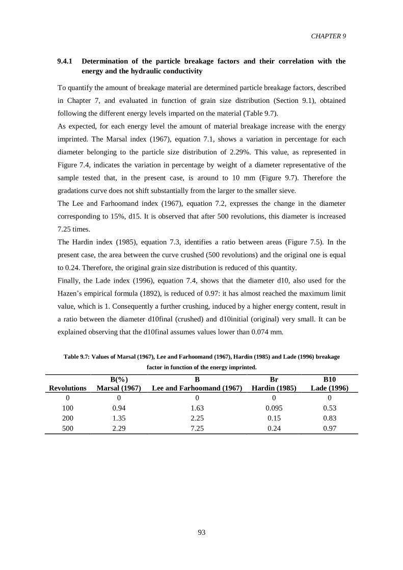
CHAPTER 9
93
9.4.1 Determination of the particle breakage factors and their correlation with the
energy and the hydraulic conductivity
To quantify the amount of breakage material are determined particle breakage factors, described
in Chapter 7, and evaluated in function of grain size distribution (Section 9.1), obtained
following the different energy levels imparted on the material (Table 9.7).
As expected, for each energy level the amount of material breakage increase with the energy
imprinted. The Marsal index (1967), equation 7.1, shows a variation in percentage for each
diameter belonging to the particle size distribution of 2.29%. This value, as represented in
Figure 7.4, indicates the variation in percentage by weight of a diameter representative of the
sample tested that, in the present case, is around to 10 mm (Figure 9.7). Therefore the
gradations curve does not shift substantially from the larger to the smaller sieve.
The Lee and Farhoomand index (1967), equation 7.2, expresses the change in the diameter
corresponding to 15%, d15. It is observed that after 500 revolutions, this diameter is increased
7.25 times.
The Hardin index (1985), equation 7.3, identifies a ratio between areas (Figure 7.5). In the
present case, the area between the curve crushed (500 revolutions) and the original one is equal
to 0.24. Therefore, the original grain size distribution is reduced of this quantity.
Finally, the Lade index (1996), equation 7.4, shows that the diameter d10, also used for the
Hazen’s empirical formula (1892), is reduced of 0.97: it has almost reached the maximum limit
value, which is 1. Consequently a further crushing, induced by a higher energy content, result in
a ratio between the diameter d10final (crushed) and d10initial (original) very small. It can be
explained observing that the d10final assumes values lower than 0.074 mm.
Table 9.7: Values of Marsal (1967), Lee and Farhoomand (1967), Hardin (1985) and Lade (1996) breakage
factor in function of the energy imprinted.
Revolutions
B(%)
Marsal (1967)
B
Lee and Farhoomand (1967)
Br
Hardin (1985)
B10
Lade (1996)
0 0 0 0 0
100 0.94 1.63 0.095 0.53
200 1.35 2.25 0.15 0.83
500 2.29 7.25 0.24 0.97

CHAPTER 9
94
Figure 9.12: Trend of Marsal breakage factor, B (%), in function of the imparted energy.
Figure 9.13: Trend of The Lee and Farhoomand breakage factor (1967) ,B, in function of the imparted
energy.
Figure 9.14: Trend of Hardin breakage factor (1985), Br, in function of the imparted energy.
0
0.5
1
1.5
2
2.5
0 100 200 300 400 500
B(%
)
Revolutions
0
1
2
3
4
5
6
7
8
0 100 200 300 400 500
B
Revolutions
0
0.05
0.1
0.15
0.2
0.25
0.3
0 100 200 300 400 500
Br
Revolutions

CHAPTER 9
95
Figure 9.15: Trend of Lade breakage factor, B10, in function of the imparted energy.
As expected, the hydraulic conductivity decreases with the amount of breakage material (Figure
9.26).
Figure 9.16: Trend between the breakage factor indexes and the hydraulic conductivity.
0
0.2
0.4
0.6
0.8
1
0 100 200 300 400 500
B10
Revolutions
0
1
2
3
4
5
6
7
8
0
0.1
0.2
0.3
0.4
0.5
0.6
0.7
0.8
0.9
1
0.001 0.01 0.1 1 10
B(%
) , B
tot
B1
0 , B
r
K [m/s]
B10totale Br (Hardin 1985) B(%)-Marsal (1967) Btotal

CHAPTER 10
96
CHAPTER 10: Conclusions
The material used for the biogas drainage layer for the nonhazardous waste landfill of Torretta,
should possess the following minimum geotechnical requirements (section 2.6 and 3.4):
Hydraulic conductivity higher than or equal to 10-4
m/s;
Grain size typical or higher than that of coarse sands.
As reported in the introduction and chapter 2, these properties are determined with the aim to
preserve the final landfill cover slope stability against the excess of pore gas pressure. In order
to determine the hydraulic conductivity must be carried out the permeability tests of the sample;
instead, to define the particle size characteristics it is necessary to perform sieve analysis.
The biogas drainage layer, as reported in the Chapter 4, is subject to various types of actions,
which can be summarized as follow:
Fracturing, attrition and wear induced by dynamic efforts explicated during the
installation and induced by grains contacts, sliding and impacts;
Compression induced by quasi-static and static load, respectively due to compaction of
the material forming the hydraulic barrier and for the weight of the overlying layers.
Due to these loads, the material forming the biogas drainage layer can arrive at failure and can
change the geotechnical requirements for which is chosen: permeability and grain size
distribution. Therefore, in order to observe if the particles of the material, due to shocks,
impacts, friction and compressions, break for fracture, attrition and abrasion, should be

CHAPTER 10
97
necessary to carried out tests able to determine its mechanical resistance (Chapter 4). Therefore,
and by the study reported in chapter 8, in order to support the efforts explicated during the
installation phase, the material must possess a certain quality which is expressed in terms of
hardness, toughness and abrasion resistance (Chapter 5). Consequently, for this purpose and in
function of the minimum grain size requirements reported in chapter 2 and 3, the Los Angeles
abrasion test appears the most suitable (section 5.2). This test is used to design roads, which for
their function and loads, are more stressed than the biogas drainage layer. Therefore, through it,
the energy transmitted to the material will be presumably greater than that present in the field.
In order to assess the ability of the material to bear stresses induced by the compaction of the
hydraulic barrier, and by the weight of the strata placed above the biogas drainage layer, should
be carried out a loading compression triaxial test (Chapter 6). In this way, it is possible to
observe whether the grains of the material due to isotropic (consolidation phase) and axial
pressure (compression phase) break changing its structure. This assumption can be made
considering that, in this second phase, the biogas drainage layer is confined and then, because of
pressure induced by the foot sheep roller, it develops vertical stresses which are comparable to
those induced by a structure on a ground and hence, solved by soil-foundation elastic theory
(section 8.1.3).
The layer in question is placed below the hydraulic barrier and then, it is not excluded the
possibility of employing a waste material, suitably selected and complies with the requirements
of acceptability of non-hazardous waste landfill. For example, in the case of exam, it is chosen a
waste incineration material (paragraph 8.2). As shown in chapter 8.2.1, is gravelly and therefore
its hydraulic conductivity is greater than the minimum required. This material, as reported in
Chapter 9, does not have a grain size for which it is possible to carry out the standard Los
Angeles abrasion and triaxial tests. Then, in order to identify its mechanical and breakage
resistance, is performed a test using the Los Angeles apparatus (chapter 9). The good results,
obtained from the acceptability analysis of the sample conducted in the laboratory, show that the
material after different shocks and dynamic stresses, of entity higher than those observed in the
situ, is able to ensure the minimum design permeability. Concluding the analyzed material can
be used as a granular medium for the biogas drainage layer: it supports the efforts explicated
during the realization of that layer and the installation of the overlying hydraulic barrier.

CHAPTER 10
98

REFERENCES
99
REFERENCES
- Alamgir, M., McDonald, Ch., Roehl, K.E., Ahsan A. (Eds.) (2005). Integrated
Management and Safe Disposal of Municipal Solid Waste in Least Deveoped Asian
Countries. A Feasibility Study. p 83. Khulna University of Engineering and
Technology, Khulna,Bangladesh;
- Al-Harti, A.A. (2001), ”A field index to determine the characteristics of crushed
aggregate”, Derpartment of Engineering and Environmental Geology, Faculty of Earth
Sciences, King Abdulaziz University, Bull Eng Geol (2001) 60:193-200;
- Al Hattamleh O. et al. (2013), “The Consequence of Particle Crushing in Engineering
Properties of Granular Materials”, International Journal of Geosciences, 2013, 4, 1055-
1060;
- Andrianatrehina et al. (2012), “Internal stability of granular materials in triaxial tests”,
ICSE6 Paris - August 27-31;
- Biarez J., Hicher P.-Y., (1997). Influence de la granulométrie et de son évolution par
ruptures de grains sur le comportement mécanique de matériaux granulaires. Revue
française de génie civil 1 (4), 607–631;
- Daouadj A., Hicher y.(2010), “An enhanced constitutive model for crushable granular
materials”, International journal for numerical and analytical methods in geomechanics,
34:555–580;
- Daouadji A, Hicher PY, Rahma A. (2001) “An elastoplastic model for granular
materials taking into account grain breakage”, European Journal of Mechanis Solids
2001; (20):113–137;
- de Graauw, A.F., van der Meulen, T., van der Does de Bye, M.R. (1984), “Granular
Filters: Design Criteria”, Journal of Waterway, Port, Coastal and Ocean Engineering,
110(1), 80-96;
- DeJong J.T., Geoffrey C. (2009), “Influence of Particle Properties and Initial Specimen
State on One-Dimensional Compression and Hydraulic Conductivity”, Journal of
Geotechnical and Geoenvironmental Engineering, Vol. 135, ASCE, 3-449–454;
- Dixon, N., Russell, D., Jones, V. (2005), “Engineering properties of municipal solid
waste”, Geotextiles and Geomembranes, 23(3), 205-233;

REFERENCES
100
- Einav, I., (2007). “Breakage mechanics—Part II: Modelling granular materials”, J.
Mech. Phys. Solids, 55 (2007) 1298–1320;
- Fernlund J.M.R. (2005), “3D image analysis size and shape method applied to the
evaluation of the Los Angeles test”, Department of Land and Water Resources
Engineering, KTH, 100 44 Stockholm, Sweden, Engineering Geology, 77, 57–67;
- Giroud, J.P., Bachus, R.C. and Bonaparte, R. (1995) “Influence of Water Flow on the
Stability of Geosynthetic-Soil Layered Systems on Slopes”,Geosynthetics International,
Vol. 2, No. 6, pp. 1149-1180;
- Göktepe A. B., A. Sezer ,(2009),“Effect of particle shape on density and permeability of
sands”, Geotechnical Engineering 163, 307-320;
- Hardin, B. O. (1985). "Crushing of soil particles", Journal of Geotechnical Engineering,
ASCE, 111(1 0), 1177- 1192;
- Hicher P.-Y., Kim M.S., Rahma A., (1995). “Experimental evidence and modelling of
grain breakage influence on mechanical behavior of granular media”, International
Workshop, “Homogenization, Theory of Migration and Granular Bodies”, Gdansk–
Kormoran, pp.125–133;
- Hu W, Yin Z Y, Dano C, et al. (2011) “A constitutive model for granular materials
considering grain breakage”, Sci China Tech Sci, 54: 2188−2196;
- Hyun Il, P., Borinara, P., Hong, K.D. (2011), “Geotechnical Considerations for End-
Use of Old Municipal SolidWaste Landfills”, International Journal of Environmantal
Research, 5(3), 573-584;
- Jessberger, H. L. (1994). “Design Procedures of Engineered Waste Landfills. Proc”.,
Meeting of Geotechnical Engineering Geotechnics in the Design and Construction of
Controlled Waste Lnadfills, Milazzo (ME), Associazione Poligeotecnici Riuniti;
- Justine Odong, (2013), “Evaluation of Empirical Formulae for Determination of
Hydraulic Conductivity based on Grain-Size Analysis”, International Journal of Agr. &
Env. [01];
- Kahraman S., Fener M. (2007), “Predicting the Los Angeles abrasion loss of rock
aggregates from the uniaxial compressive strength”, Mining Engineering Department,
Nigde University, 51100 Nigde, Turkey, Geological Engineering Department, Nigde
University, 01330 Nigde, Turkey, 4861–4865;
- Kenney, T.C., Lau, D. (1986), “Internal stability of granular filters: Reply”, Canadian
Geotechnical Journal, 23(3), 420-423;
- Kezdi, A. (1969), “Increase of protective capacity of flood control dikes”, Department
of Geotechnique, Technical University, Budapest, Hungary;

REFERENCES
101
- Lade P.V., Yamamuro A., Bopp Paul A., (1996), “Significance of particle crushing in
granular materials”, Journal of Geotechnical Engineering, ASCE, 122:309-316;
- Lee K.L., Farhoomand I., (1967). “Compressibility and crushing of granular soils in
anisotropic triaxial compression”, Canadian Geotechnical Journal, Vol. 4, No. 1, 1967,
pp. 68-86;
- Marsal R.J., (1967). “Large scale testing of rockfill materials”, Journal of the Soil
Mechanics and Foundations Division 93 (SM2), 27–43;
- Millard, R.S. (1993). Road building in the Tropics. Transport Research Laboratory
State-of-the-art Review 9, HMSO, London;
- Moraci, N., Tondello, M. (1996), “La progettazione dei filtri nell’ingegneria marittima”,
Atti IV Convegno AIOM, Padova;
- Musso, A., Federico, F. (1983), “Un metodo geometrico-probabilistico per la verifica
dei filtri”, Rivista Italiana di Geotecnica, 4, 177-193;
- Raut, A.K. (2006), “Mathematical modelling of granular filters and constriction-based
filter design criteria”, PhD Thesis, University of Wollongong, Australia;
- Thiel, R.S. (1998), “Design and Testing of a NWNP Geotextile Gas Pressure Relief
Layer Below a Geomembrane Cover to Improve Slope Stability”, Geosynthetics
International;
- Thiel, R.S. (1998), “Design Methodology for a Gas Pressure Relief Layer Below a
Geomembrane Landfill Cover to Improve Slope Stability”, Geosynthetics International,
5(6), 589-617;
- Ugur et. al.(2010) “Effect of rock properties on the Los Angeles abrasion and impact
test characteristics of the aggregates”, materials characterization,61 ,90-96;
- Wan, C.F., Fell, R. (2008), “Assessing the Potential of Internal Instability and Suffusion
in Embankment Dams and Their Foundations”, Journal of Geotechnical and
Geoenvironmental Engineering, 134(3), 401-407.
- Decreto legislative 36 del 13/01/2003;
- Decreto Legislativo 13 gennaio 2003, n. 36: www.camera.it;
- Decreto ministeriale 11 marzo 1988: www.attiministeriali.miur.it;
- Bonaparte et. al. (2004), “(Draft) Technical Guidance, For RCRA/CERCLA Final
Covers, EPA;
- ISRM (1998). “Metodi suggeriti per a determinazione della durezza e dell’abrasività
delle rocce”, Rivista italiana di geotecnica 2, 64-70;
REFERENCES
102
- SS (1974). SS73:1974 “Specification for methods for sampling and testing of mineral
aggregates, sand and fillers” - Determination of aggregate impact value, aggregate
crushing value and ten percent fines value. Singapore Standard, Singapore.
- UNI EN 1097-2:2010;
- Colombo P. e Colleselli F., (2012), “Elementi di geotecnica” , Zanichelli;
- Harold N. Atkins, (2003), “Highway materials, Soils and Concretes”, Prentice Hall;
- Yang H. Haung, (2003), “Pavement Analysis and Design (3rd
edition)”, Prentice Hall.
- Favaretti M.: “Environmental geotechnics”. Academic year 2012-2013, Università degli
studi di Padova.
- Busana S. : Progetto preliminare della copertura superficiale finale della discarica di
rifiuti urbani e/o non pericolosi di Torretta (Legnago), 2015;
- Cover Slope Stability: Landfill Gas Pressure: www.ladfilldesign.com;
- Landfill gas pressure relief layer: www.ladfilldesign.com;
- Slope stability sensitivities of final covers: www.geosyntheticsmagazine.com .